Embed Size (px)
Citation preview
Finite Fields and Their Applications 10 (2004) 464–479
Matrix-product constructions of digital nets
Harald Niederreitera,� and Ferruh Ozbudakb
aDepartment of Mathematics, National University of Singapore, 2 Science Drive 2, Singapore 117543,
Republic of SingaporebDepartment of Mathematics, Middle East Technical University, ’Inonu Bulvarı, 06531, Ankara, Turkey
Received 2 October 2003
Communicated by Peter Shiue
Abstract
We present a new construction of digital nets, and more generally of ðd; k;m; sÞ-systems,
over finite fields which is an analog of the matrix-product construction of codes. Examples
show that this construction can yield digital nets with better parameters compared to
competing constructions.
r 2004 Elsevier Inc. All rights reserved.
Keywords: Digital nets; Matrix-product construction of codes; Quasi-Monte Carlo methods
1. Introduction
Digital ðt;m; sÞ-nets arise and are used in s-dimensional quasi-Monte Carlointegration as point sets in the s-dimensional unit cube with excellent uniformityproperties (see [3,5, Chapter 4; 10, Chapter 8]). Although digital ðt;m; sÞ-nets can beconstructed by means of arbitrary finite commutative rings with identity, we focushere on the special case of constructions with the help of a finite field Fq; where
q is an arbitrary prime power. In this special case we speak of a digital ðt;m; sÞ-net
over Fq:
Digital ðt;m; sÞ-nets over Fq can equivalently be described in terms of certain
systems of vectors in the Fq-linear space Fmq : These systems of vectors should have
special linear independence properties. It will be convenient to adopt a somewhatmore general perspective on these systems of vectors which stems from [4,8].
ARTICLE IN PRESS
�Corresponding author. Fax: +65-6779-5452.
E-mail addresses: [email protected] (H. Niederreiter), [email protected] (F. Ozbudak).
1071-5797/$ - see front matter r 2004 Elsevier Inc. All rights reserved.
doi:10.1016/j.ffa.2003.11.004
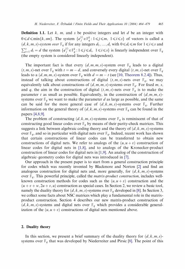
Definition 1.1. Let k; m; and s be positive integers and let d be an integer with
0pdpminfk; smg: The system fcðiÞj AFk
q : 1pjpm; 1pipsg of vectors is called a
ðd; k;m; sÞ-system over Fq if for any integers d1;y; ds with 0pdipm for 1pips andPsi¼1 di ¼ d the system fc
ðiÞj AFk
q : 1pjpdi; 1pipsg is linearly independent over Fq
(the empty system is considered linearly independent).
The important fact is that every ðd;m;m; sÞ-system over Fq leads to a digital
ðt;m; sÞ-net over Fq with t ¼ m � d; and conversely every digital ðt;m; sÞ-net over Fq
leads to a ðd;m;m; sÞ-system over Fq with d ¼ m � t (see [10, Theorem 8.2.4]). Thus,
instead of talking about constructions of digital ðt;m; sÞ-nets over Fq; we may
equivalently talk about constructions of ðd;m;m; sÞ-systems over Fq: For fixed m; s;
and q; the aim in the construction of digital ðt;m; sÞ-nets over Fq is to make the
parameter t as small as possible. Equivalently, in the construction of ðd;m;m; sÞ-systems over Fq we want to make the parameter d as large as possible, and the same
can be said for the more general case of ðd; k;m; sÞ-systems over Fq: Further
information on the general theory of ðd; k;m; sÞ-systems over Fq can be found in the
papers [4,8,9].The problem of constructing ðd; k;m; sÞ-systems over Fq is reminiscent of that of
constructing good linear codes over Fq by means of their parity-check matrices. This
suggests a link between algebraic coding theory and the theory of ðd; k;m; sÞ-systemsover Fq; and so in particular with digital nets over Fq: Indeed, recent work has shown
that certain constructions of linear codes can be transferred to obtain newconstructions of digital nets. We refer to analogs of the ðu; u þ vÞ construction oflinear codes for digital nets in [1,8], and to analogs of the Kronecker-productconstruction of linear codes for digital nets in [1,9]. An analog of the construction ofalgebraic–geometry codes for digital nets was introduced in [7].
Our approach in the present paper is to start from a general construction principlefor codes which was recently invented by Blackmore and Norton [2] and find ananalogous construction for digital nets and, more generally, for ðd; k;m; sÞ-systemsover Fq: This powerful principle, called the matrix-product construction, includes well-
known construction methods for codes such as the ðu; u þ vÞ construction and theðu þ v þ w; 2u þ v; uÞ construction as special cases. In Section 2, we review a basic tool,namely the duality theory for ðd; k;m; sÞ-systems over Fq developed in [8]. In Section 3,
we collect some facts about NSC matrices which play a fundamental role in the matrix-product construction. Section 4 describes our new matrix-product construction ofðd; k;m; sÞ-systems and digital nets over Fq which provides a considerable general-
ization of the ðu; u þ vÞ constructions of digital nets mentioned above.
2. Duality theory
In this section, we present a brief summary of the duality theory for ðd; k;m; sÞ-systems over Fq that was developed by Niederreiter and Pirsic [8]. The point of this
ARTICLE IN PRESS
H. Niederreiter, F. .Ozbudak / Finite Fields and Their Applications 10 (2004) 464–479 465
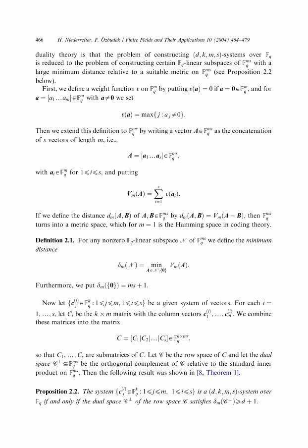
duality theory is that the problem of constructing ðd; k;m; sÞ-systems over Fq
is reduced to the problem of constructing certain Fq-linear subspaces of Fmsq with a
large minimum distance relative to a suitable metric on Fmsq (see Proposition 2.2
below).First, we define a weight function v on Fm
q by putting vðaÞ ¼ 0 if a ¼ 0AFmq ; and for
a ¼ ½a1yamAFmq with aa0 we set
vðaÞ ¼ maxf j : a ja0g:
Then we extend this definition to Fmsq by writing a vector AAFms
q as the concatenation
of s vectors of length m; i.e.,
A ¼ ½a1yasAFmsq ;
with aiAFmq for 1pips; and putting
VmðAÞ ¼Xs
i¼1
vðaiÞ:
If we define the distance dmðA;BÞ of A;BAFmsq by dmðA;BÞ ¼ VmðA � BÞ; then Fms
q
turns into a metric space, which for m ¼ 1 is the Hamming space in coding theory.
Definition 2.1. For any nonzero Fq-linear subspace N of Fmsq we define the minimum
distance
dmðNÞ ¼ minAAN\f0g
VmðAÞ:
Furthermore, we put dmðf0gÞ ¼ ms þ 1:
Now let fcðiÞj AFk
q : 1pjpm; 1pipsg be a given system of vectors. For each i ¼1;y; s; let Ci be the k � m matrix with the column vectors c
ðiÞ1 ;y; c
ðiÞm : We combine
these matrices into the matrix
C ¼ ½C1jC2jyjCsAFk�msq ;
so that C1;y;Cs are submatrices of C: Let C be the row space of C and let the dual
space C>DFmsq be the orthogonal complement of C relative to the standard inner
product on Fmsq : Then the following result was shown in [8, Theorem 1].
Proposition 2.2. The system fcðiÞj AFk
q : 1pjpm; 1pipsg is a ðd; k;m; sÞ-system over
Fq if and only if the dual space C> of the row space C satisfies dmðC>ÞXd þ 1:
ARTICLE IN PRESS
H. Niederreiter, F. .Ozbudak / Finite Fields and Their Applications 10 (2004) 464–479466
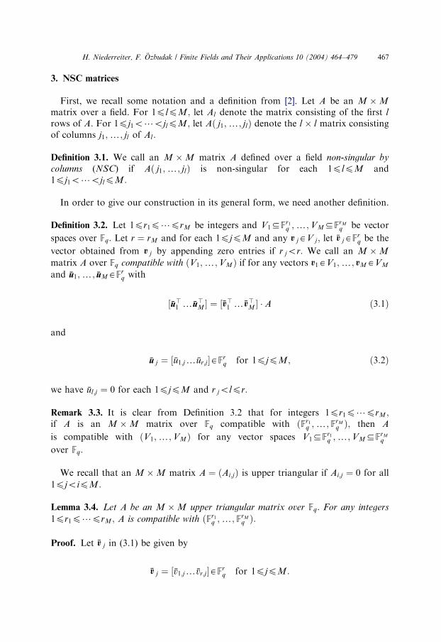
3. NSC matrices
First, we recall some notation and a definition from [2]. Let A be an M � M
matrix over a field. For 1plpM; let Al denote the matrix consisting of the first l
rows of A: For 1pj1o?ojlpM; let Að j1;y; jlÞ denote the l � l matrix consistingof columns j1;y; jl of Al :
Definition 3.1. We call an M � M matrix A defined over a field non-singular by
columns (NSC) if Að j1;y; jlÞ is non-singular for each 1plpM and1pj1o?ojlpM:
In order to give our construction in its general form, we need another definition.
Definition 3.2. Let 1pr1p?prM be integers and V1DFr1q ;y;VMDFrM
q be vector
spaces over Fq: Let r ¼ rM and for each 1pjpM and any v jAV j; let %v jAFrq be the
vector obtained from v j by appending zero entries if r jor: We call an M � M
matrix A over Fq compatible with ðV1;y;VMÞ if for any vectors v1AV1;y; vMAVM
and %u1;y; %uMAFrq with
½%u?1 y%u?
M ¼ ½%v?1 y%v?M A ð3:1Þ
and
%u j ¼ ½ %u1;jy %ur;jAFrq for 1pjpM; ð3:2Þ
we have %ul;j ¼ 0 for each 1pjpM and r jolpr:
Remark 3.3. It is clear from Definition 3.2 that for integers 1pr1p?prM ;if A is an M � M matrix over Fq compatible with ðFr1
q ;y; FrMq Þ; then A
is compatible with ðV1;y;VMÞ for any vector spaces V1DFr1q ;y;VMDFrM
q
over Fq:
We recall that an M � M matrix A ¼ ðAi;jÞ is upper triangular if Ai;j ¼ 0 for all
1pjoipM:
Lemma 3.4. Let A be an M � M upper triangular matrix over Fq: For any integers
1pr1p?prM ; A is compatible with ðFr1q ;y; FrM
q Þ:
Proof. Let %v j in (3.1) be given by
%v j ¼ ½%v1;jy%vr;jAFrq for 1pjpM:
ARTICLE IN PRESS
H. Niederreiter, F. .Ozbudak / Finite Fields and Their Applications 10 (2004) 464–479 467
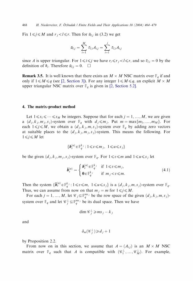
Fix 1pjpM and r jolpr: Then for %ul;j in (3.2) we get
%ul;j ¼XMi¼1
%vl;iAi;j ¼Xj
i¼1
%vl;iAi;j
since A is upper triangular. For 1pipj we have ripr jolpr; and so %vl;i ¼ 0 by the
definition of %vi: Therefore %ul;j ¼ 0: &
Remark 3.5. It is well known that there exists an M � M NSC matrix over Fq if and
only if 1pMpq (see [2, Section 3]). For any integer 1pMpq; an explicit M � M
upper triangular NSC matrix over Fq is given in [2, Section 5.2].
4. The matrix-product method
Let 1ps1p?psM be integers. Suppose that for each j ¼ 1;y;M; we are givena ðd j; k j;m j; s jÞ-system over Fq with d jpm j: Put m ¼ maxfm1;y;mMg: For
each 1pjpM; we obtain a ðd j ; k j;m; s jÞ-system over Fq by adding zero vectors
at suitable places to the ðd j; k j;m j; s jÞ-system. This means the following. For
1pjpM let
fbðuÞv AFk j
q : 1pvpm j ; 1pups jg
be the given ðd j; k j;m j; s jÞ-system over Fq: For 1pvpm and 1pups j let
%bðuÞv ¼
bðuÞv AFk j
q if 1pvpm j ;
0AFk jq if m jovpm:
(ð4:1Þ
Then the system f%bðuÞv AFk j
q : 1pvpm; 1pups jg is a ðd j; k j;m; s jÞ-system over Fq:
Thus, we can assume from now on that m j ¼ m for 1pjpM:
For each j ¼ 1;y;M; let C jDFms jq be the row space of the given ðd j; k j;m; s jÞ-
system over Fq and let C>j DFms j
q be its dual space. Then we have
dimC>j Xms j � k j
and
dmðC>j ÞXd j þ 1
by Proposition 2.2.From now on in this section, we assume that A ¼ ðAi;jÞ is an M � M NSC
matrix over Fq such that A is compatible with ðC>1 ;y;C>
MÞ: For example,
ARTICLE IN PRESS
H. Niederreiter, F. .Ozbudak / Finite Fields and Their Applications 10 (2004) 464–479468
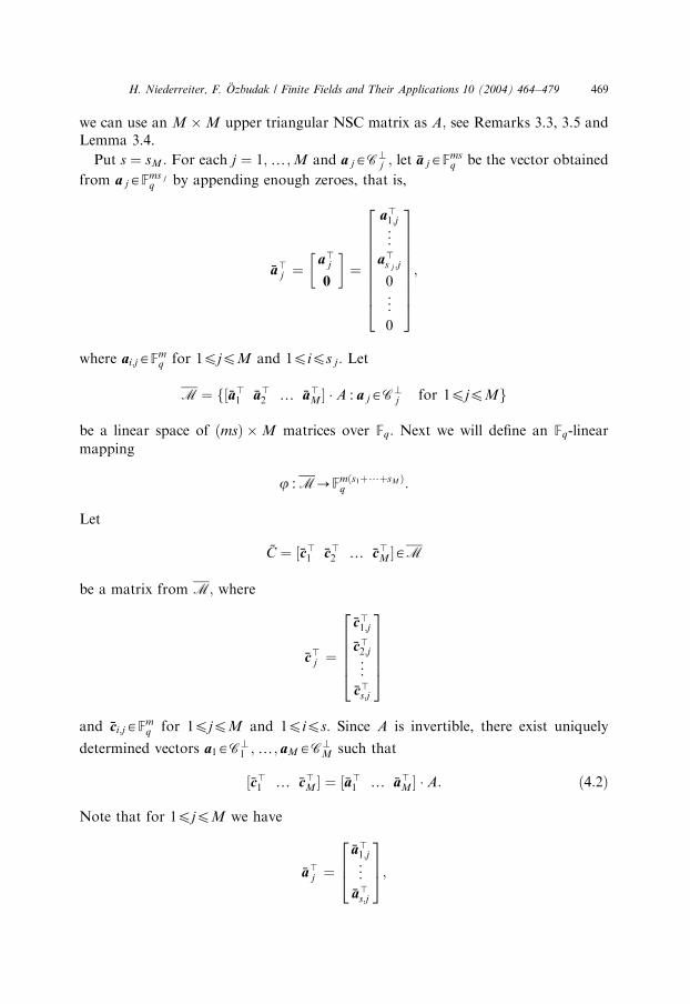
we can use an M � M upper triangular NSC matrix as A; see Remarks 3.3, 3.5 andLemma 3.4.
Put s ¼ sM : For each j ¼ 1;y;M and a jAC>j ; let %a jAFms
q be the vector obtained
from a jAFms jq by appending enough zeroes, that is,
%a?j ¼
a?j
0
� �¼
a?1;j
^
a?s j ;j
0
^
0
2666666664
3777777775;
where ai;jAFmq for 1pjpM and 1pips j: Let
M ¼ f½%a?1 %a?
2 y %a?M A : a jAC>
j for 1pjpMg
be a linear space of ðmsÞ � M matrices over Fq: Next we will define an Fq-linear
mapping
j :M-Fmðs1þ?þsM Þq :
Let
%C ¼ ½%c?1 %c?2 y %c?M AM
be a matrix from M; where
%c?j ¼
%c?1;j
%c?2;j^
%c?s;j
266664377775
and %ci;jAFmq for 1pjpM and 1pips: Since A is invertible, there exist uniquely
determined vectors a1AC>1 ;y; aMAC>
M such that
½%c?1 y %c?M ¼ ½%a?1 y %a?
M A: ð4:2Þ
Note that for 1pjpM we have
%a?j ¼
%a?1;j
^
%a?s;j
264375;
ARTICLE IN PRESS
H. Niederreiter, F. .Ozbudak / Finite Fields and Their Applications 10 (2004) 464–479 469
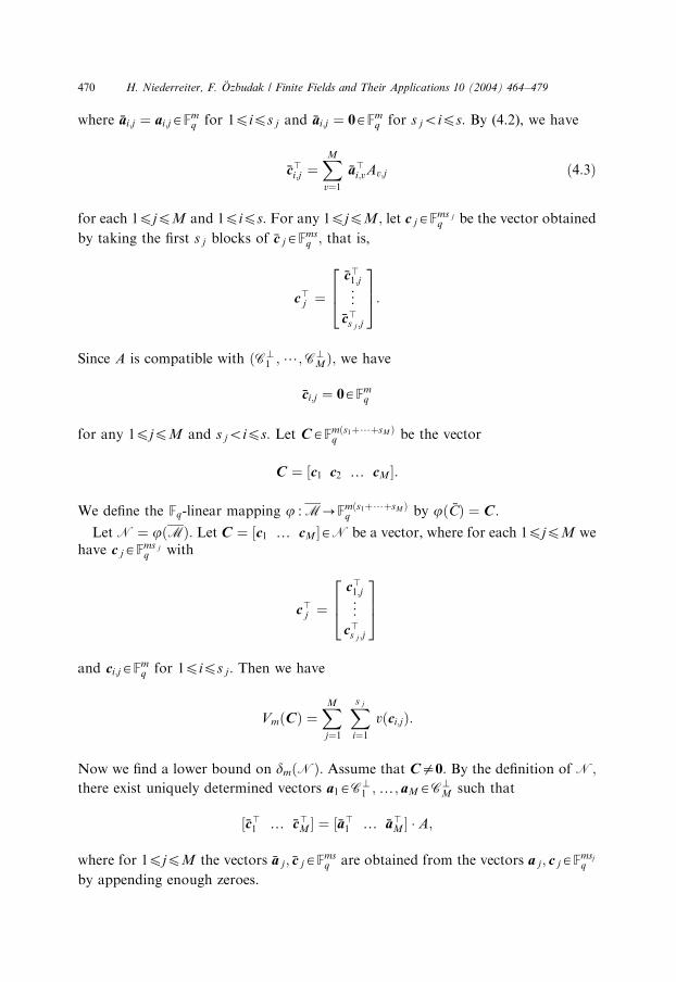
where %ai;j ¼ ai;jAFmq for 1pips j and %ai;j ¼ 0AFm
q for s joips: By (4.2), we have
%c?i;j ¼XM
v¼1
%a?i;vAv;j ð4:3Þ
for each 1pjpM and 1pips: For any 1pjpM; let c jAFms jq be the vector obtained
by taking the first s j blocks of %c jAFmsq ; that is,
c?j ¼%c?1;j^
%c?s j ;j
264375:
Since A is compatible with ðC>1 ;?;C>
MÞ; we have
%ci;j ¼ 0AFmq
for any 1pjpM and s joips: Let CAFmðs1þ?þsM Þq be the vector
C ¼ ½c1 c2 y cM :
We define the Fq-linear mapping j :M-Fmðs1þ?þsM Þq by jð %CÞ ¼ C :
Let N ¼ jðMÞ: Let C ¼ ½c1 y cM AN be a vector, where for each 1pjpM wehave c jAFms j
q with
c?j ¼c?1;j^
c?s j ;j
264375
and ci;jAFmq for 1pips j: Then we have
VmðCÞ ¼XM
j¼1
Xs j
i¼1
vðci;jÞ:
Now we find a lower bound on dmðNÞ: Assume that Ca0: By the definition of N;
there exist uniquely determined vectors a1AC>1 ;y; aMAC>
M such that
½%c?1 y %c?M ¼ ½%a?1 y %a?
M A;
where for 1pjpM the vectors %a j; %c jAFmsq are obtained from the vectors a j; c jAFmsj
q
by appending enough zeroes.
ARTICLE IN PRESS
H. Niederreiter, F. .Ozbudak / Finite Fields and Their Applications 10 (2004) 464–479470
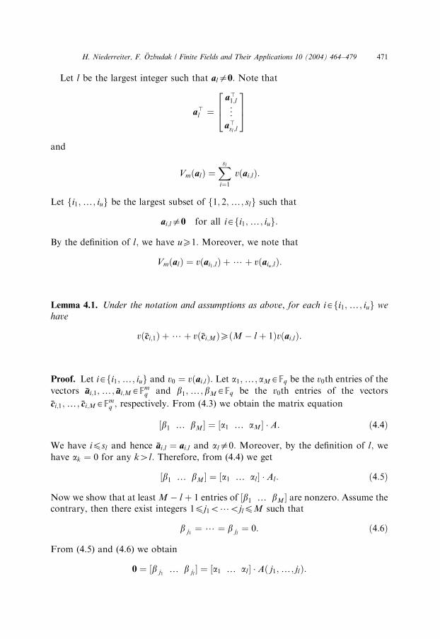
Let l be the largest integer such that ala0: Note that
a?l ¼
a?1;l
^
a?sl ;l
264375
and
VmðalÞ ¼Xsl
i¼1
vðai;lÞ:
Let fi1;y; iug be the largest subset of f1; 2;y; slg such that
ai;la0 for all iAfi1;y; iug:
By the definition of l; we have uX1: Moreover, we note that
VmðalÞ ¼ vðai1;lÞ þ?þ vðaiu;lÞ:
Lemma 4.1. Under the notation and assumptions as above, for each iAfi1;y; iug we
have
vð%ci;1Þ þ?þ vð%ci;MÞXðM � l þ 1Þvðai;lÞ:
Proof. Let iAfi1;y; iug and v0 ¼ vðai;lÞ: Let a1;y; aMAFq be the v0th entries of the
vectors %ai;1;y; %ai;MAFmq and b1;y; bMAFq be the v0th entries of the vectors
%ci;1;y; %ci;MAFmq ; respectively. From (4.3) we obtain the matrix equation
½b1 y bM ¼ ½a1 y aM A: ð4:4Þ
We have ipsl and hence %ai;l ¼ ai;l and ala0: Moreover, by the definition of l; wehave ak ¼ 0 for any k4l: Therefore, from (4.4) we get
½b1 y bM ¼ ½a1 y al Al : ð4:5Þ
Now we show that at least M � l þ 1 entries of ½b1 y bM are nonzero. Assume thecontrary, then there exist integers 1pj1o?ojlpM such that
b j1¼ ? ¼ b jl
¼ 0: ð4:6Þ
From (4.5) and (4.6) we obtain
0 ¼ ½b j1y b jl
¼ ½a1 y al Að j1;y; jlÞ:
ARTICLE IN PRESS
H. Niederreiter, F. .Ozbudak / Finite Fields and Their Applications 10 (2004) 464–479 471
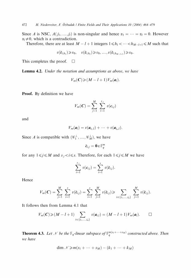
Since A is NSC, Að j1;y; jlÞ is non-singular and hence a1 ¼ ? ¼ al ¼ 0: Howeverala0; which is a contradiction.
Therefore, there are at least M � l þ 1 integers 1ph1o?ohM�lþ1pM such that
vð%ci;h1ÞXv0; vð%ci;h2ÞXv0;y; vð%ci;hM�lþ1ÞXv0:
This completes the proof. &
Lemma 4.2. Under the notation and assumptions as above, we have
VmðCÞXðM � l þ 1ÞVmðalÞ:
Proof. By definition we have
VmðCÞ ¼XM
j¼1
Xs j
i¼1
vðci;jÞ
and
VmðalÞ ¼ vðai1;lÞ þ?þ vðaiu;lÞ:
Since A is compatible with ðC>1 ;y;C>
MÞ; we have
%ci;j ¼ 0AFmq
for any 1pjpM and s joips: Therefore, for each 1pjpM we have
Xs j
i¼1
vðci;jÞ ¼Xs
i¼1
vð%ci;jÞ:
Hence
VmðCÞ ¼XM
j¼1
Xs
i¼1
vð%ci;jÞ ¼Xs
i¼1
XM
j¼1
vð%ci;jÞXX
iAfi1;y;iug
XM
j¼1
vð%ci;jÞ:
It follows then from Lemma 4.1 that
VmðCÞXðM � l þ 1ÞX
iAfi1;y;iugvðai;lÞ ¼ ðM � l þ 1ÞVmðalÞ: &
Theorem 4.3. Let N be the Fq-linear subspace of Fmðs1þ?þsM Þq constructed above. Then
we have
dimNXmðs1 þ?þ sMÞ � ðk1 þ?þ kMÞ
ARTICLE IN PRESS
H. Niederreiter, F. .Ozbudak / Finite Fields and Their Applications 10 (2004) 464–479472
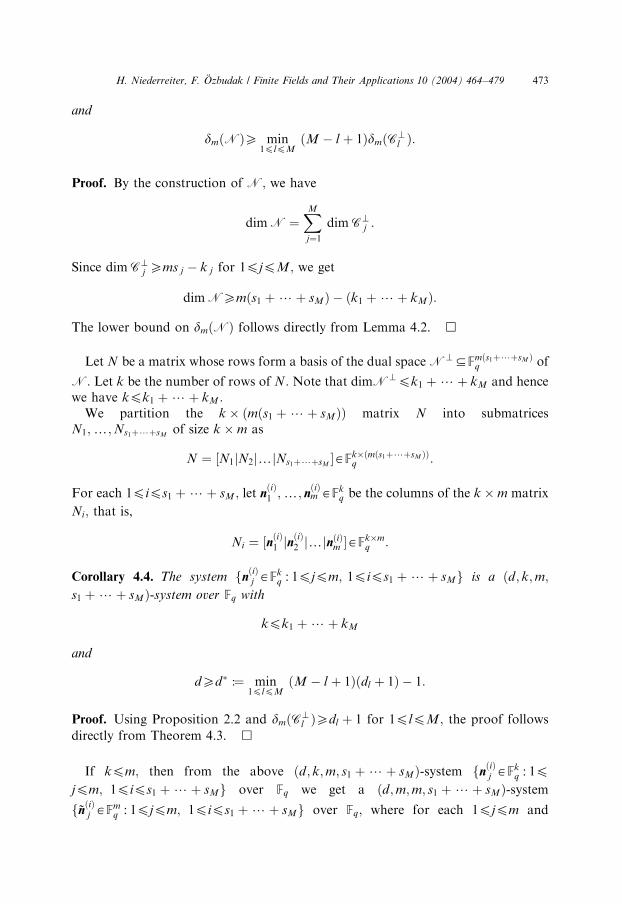
and
dmðNÞX min1plpM
ðM � l þ 1ÞdmðC>l Þ:
Proof. By the construction of N; we have
dimN ¼XM
j¼1
dimC>j :
Since dimC>j Xms j � k j for 1pjpM; we get
dimNXmðs1 þ?þ sMÞ � ðk1 þ?þ kMÞ:
The lower bound on dmðNÞ follows directly from Lemma 4.2. &
Let N be a matrix whose rows form a basis of the dual space N>DFmðs1þ?þsM Þq of
N: Let k be the number of rows of N: Note that dimN>pk1 þ?þ kM and hencewe have kpk1 þ?þ kM :
We partition the k � ðmðs1 þ?þ sMÞÞ matrix N into submatricesN1;y;Ns1þ?þsM
of size k � m as
N ¼ ½N1jN2jyjNs1þ?þsMAFk�ðmðs1þ?þsM ÞÞ
q :
For each 1pips1 þ?þ sM ; let nðiÞ1 ;y; n
ðiÞm AFk
q be the columns of the k � m matrix
Ni; that is,
Ni ¼ ½nðiÞ1 jnðiÞ
2 jyjnðiÞm AFk�m
q :
Corollary 4.4. The system fnðiÞj AFk
q : 1pjpm; 1pips1 þ?þ sMg is a ðd; k;m;
s1 þ?þ sMÞ-system over Fq with
kpk1 þ?þ kM
and
dXd� :¼ min1plpM
ðM � l þ 1Þðdl þ 1Þ � 1:
Proof. Using Proposition 2.2 and dmðC>l ÞXdl þ 1 for 1plpM; the proof follows
directly from Theorem 4.3. &
If kpm; then from the above ðd; k;m; s1 þ?þ sMÞ-system fnðiÞj AFk
q : 1pjpm; 1pips1 þ?þ sMg over Fq we get a ðd;m;m; s1 þ?þ sMÞ-systemf*nðiÞ
j AFmq : 1pjpm; 1pips1 þ?þ sMg over Fq; where for each 1pjpm and
ARTICLE IN PRESS
H. Niederreiter, F. .Ozbudak / Finite Fields and Their Applications 10 (2004) 464–479 473
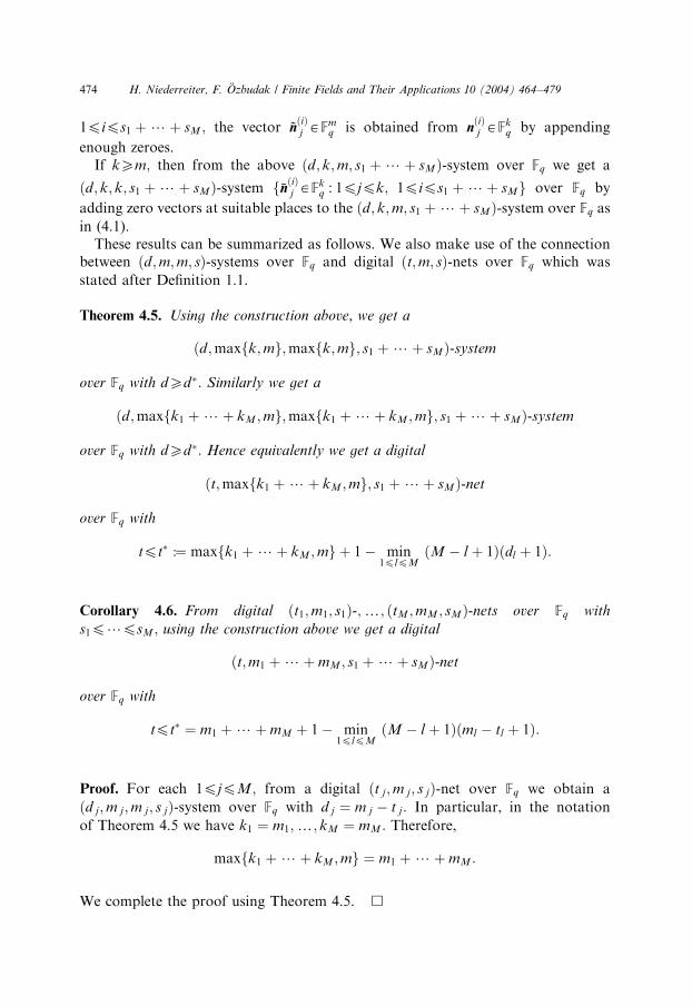
1pips1 þ?þ sM ; the vector *nðiÞj AFm
q is obtained from nðiÞj AFk
q by appending
enough zeroes.If kXm; then from the above ðd; k;m; s1 þ?þ sMÞ-system over Fq we get a
ðd; k; k; s1 þ?þ sMÞ-system f%nðiÞj AFk
q : 1pjpk; 1pips1 þ?þ sMg over Fq by
adding zero vectors at suitable places to the ðd; k;m; s1 þ?þ sMÞ-system over Fq as
in (4.1).These results can be summarized as follows. We also make use of the connection
between ðd;m;m; sÞ-systems over Fq and digital ðt;m; sÞ-nets over Fq which was
stated after Definition 1.1.
Theorem 4.5. Using the construction above, we get a
ðd;maxfk;mg;maxfk;mg; s1 þ?þ sMÞ-system
over Fq with dXd�: Similarly we get a
ðd;maxfk1 þ?þ kM ;mg;maxfk1 þ?þ kM ;mg; s1 þ?þ sMÞ-system
over Fq with dXd�: Hence equivalently we get a digital
ðt;maxfk1 þ?þ kM ;mg; s1 þ?þ sMÞ-net
over Fq with
tpt� :¼ maxfk1 þ?þ kM ;mg þ 1� min1plpM
ðM � l þ 1Þðdl þ 1Þ:
Corollary 4.6. From digital ðt1;m1; s1Þ-;y; ðtM ;mM ; sMÞ-nets over Fq with
s1p?psM ; using the construction above we get a digital
ðt;m1 þ?þ mM ; s1 þ?þ sMÞ-net
over Fq with
tpt� ¼ m1 þ?þ mM þ 1� min1plpM
ðM � l þ 1Þðml � tl þ 1Þ:
Proof. For each 1pjpM; from a digital ðt j;m j; s jÞ-net over Fq we obtain a
ðd j;m j;m j; s jÞ-system over Fq with d j ¼ m j � t j: In particular, in the notation
of Theorem 4.5 we have k1 ¼ m1;y; kM ¼ mM : Therefore,
maxfk1 þ?þ kM ;mg ¼ m1 þ?þ mM :
We complete the proof using Theorem 4.5. &
ARTICLE IN PRESS
H. Niederreiter, F. .Ozbudak / Finite Fields and Their Applications 10 (2004) 464–479474

Example 4.7. Let Fq be an arbitrary finite field, let M ¼ 2; and let
A ¼1 1
0 1
� �:
It is clear that A is an upper triangular NSC matrix over Fq: Let a digital ðt1;m1; s1Þ-net over Fq and a digital ðt2;m2; s2Þ-net over Fq with s1ps2 be given. Then Corollary
4.6 yields a digital ðt;m1 þ m2; s1 þ s2Þ-net over Fq with
tpt� ¼ m1 þ m2 þ 1�minf2ðm1 � t1 þ 1Þ;m2 � t2 þ 1g:
If we now assume that m2 � t2 þ 1p2ðm1 � t1 þ 1Þ; then t� ¼ m1 þ t2: This yieldsexactly the result of [1, Corollary 5.1]. Thus, our construction is more general thanthe ðu; u þ vÞ construction in [1, Section 5].
Example 4.8. Let Fq be a finite field with qX3; let M ¼ 3; and let
A ¼1 2 1
0 1 1
0 0 1
264375:
It is clear that A is an upper triangular NSC matrix over Fq: For each i ¼ 1; 2; 3;
let a digital ðti;mi; siÞ-net over Fq be given, where s1ps2ps3: Then by
Corollary 4.6 we obtain a digital ðt;m1 þ m2 þ m3; s1 þ s2 þ s3Þ-net over Fq
with
tpt� ¼ m1 þ m2 þ m3 þ 1�minf3ðm1 � t1 þ 1Þ; 2ðm2 � t2 þ 1Þ;m3 � t3 þ 1g:
This yields a new propagation rule for digital nets; compare with [6, Section 3] for alist of propagation rules for (digital) nets.
Remark 4.9. The ordering s1p?psM is important. Consider digital ðt1;m1; s1Þ-,ðt2;m2; s2Þ-, and ðt3;m3; s3Þ-nets over Fq with s1ps2ps3: There are some alternatives
to construct a digital ðt;m1 þ m2 þ m3; s1 þ s2 þ s3Þ-net over Fq applying the
construction of this section.Case I: Using Example 4.8, we obtain a digital ðtð1;2;3Þ;m1 þ m2 þ m3; s1 þ s2 þ s3Þ-
net over Fq with
tð1;2;3Þpt�ð1;2;3Þ ¼m1 þ m2 þ m3 þ 1
� minf3ðm1 � t1 þ 1Þ; 2ðm2 � t2 þ 1Þ;m3 � t3 þ 1g:
In this case, but not in the following two cases, we have to assume that qX3:
ARTICLE IN PRESS
H. Niederreiter, F. .Ozbudak / Finite Fields and Their Applications 10 (2004) 464–479 475
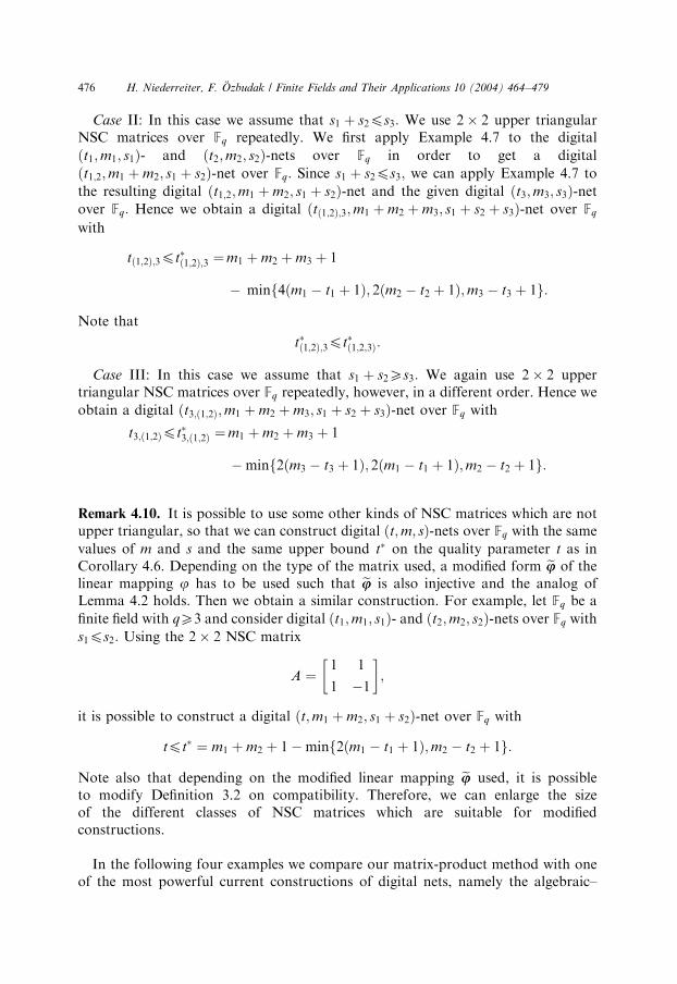
Case II: In this case we assume that s1 þ s2ps3: We use 2� 2 upper triangularNSC matrices over Fq repeatedly. We first apply Example 4.7 to the digital
ðt1;m1; s1Þ- and ðt2;m2; s2Þ-nets over Fq in order to get a digital
ðt1;2;m1 þ m2; s1 þ s2Þ-net over Fq: Since s1 þ s2ps3; we can apply Example 4.7 to
the resulting digital ðt1;2;m1 þ m2; s1 þ s2Þ-net and the given digital ðt3;m3; s3Þ-netover Fq: Hence we obtain a digital ðtð1;2Þ;3;m1 þ m2 þ m3; s1 þ s2 þ s3Þ-net over Fq
with
tð1;2Þ;3pt�ð1;2Þ;3 ¼m1 þ m2 þ m3 þ 1
� minf4ðm1 � t1 þ 1Þ; 2ðm2 � t2 þ 1Þ;m3 � t3 þ 1g:
Note that
t�ð1;2Þ;3pt�ð1;2;3Þ:
Case III: In this case we assume that s1 þ s2Xs3: We again use 2� 2 uppertriangular NSC matrices over Fq repeatedly, however, in a different order. Hence we
obtain a digital ðt3;ð1;2Þ;m1 þ m2 þ m3; s1 þ s2 þ s3Þ-net over Fq with
t3;ð1;2Þpt�3;ð1;2Þ ¼m1 þ m2 þ m3 þ 1
�minf2ðm3 � t3 þ 1Þ; 2ðm1 � t1 þ 1Þ;m2 � t2 þ 1g:
Remark 4.10. It is possible to use some other kinds of NSC matrices which are notupper triangular, so that we can construct digital ðt;m; sÞ-nets over Fq with the same
values of m and s and the same upper bound t� on the quality parameter t as inCorollary 4.6. Depending on the type of the matrix used, a modified form ejj of thelinear mapping j has to be used such that ejj is also injective and the analog ofLemma 4.2 holds. Then we obtain a similar construction. For example, let Fq be a
finite field with qX3 and consider digital ðt1;m1; s1Þ- and ðt2;m2; s2Þ-nets over Fq with
s1ps2: Using the 2� 2 NSC matrix
A ¼1 1
1 �1
� �;
it is possible to construct a digital ðt;m1 þ m2; s1 þ s2Þ-net over Fq with
tpt� ¼ m1 þ m2 þ 1�minf2ðm1 � t1 þ 1Þ;m2 � t2 þ 1g:
Note also that depending on the modified linear mapping ejj used, it is possibleto modify Definition 3.2 on compatibility. Therefore, we can enlarge the sizeof the different classes of NSC matrices which are suitable for modifiedconstructions.
In the following four examples we compare our matrix-product method with oneof the most powerful current constructions of digital nets, namely the algebraic–
ARTICLE IN PRESS
H. Niederreiter, F. .Ozbudak / Finite Fields and Their Applications 10 (2004) 464–479476
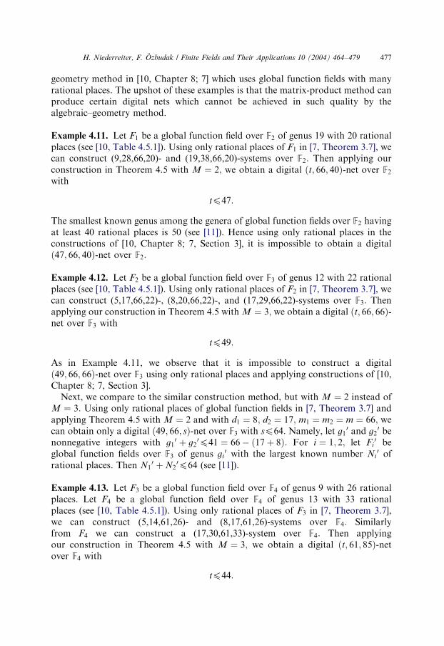
geometry method in [10, Chapter 8; 7] which uses global function fields with manyrational places. The upshot of these examples is that the matrix-product method canproduce certain digital nets which cannot be achieved in such quality by thealgebraic–geometry method.
Example 4.11. Let F1 be a global function field over F2 of genus 19 with 20 rationalplaces (see [10, Table 4.5.1]). Using only rational places of F1 in [7, Theorem 3.7], wecan construct (9,28,66,20)- and (19,38,66,20)-systems over F2: Then applying ourconstruction in Theorem 4.5 with M ¼ 2; we obtain a digital ðt; 66; 40Þ-net over F2with
tp47:
The smallest known genus among the genera of global function fields over F2 havingat least 40 rational places is 50 (see [11]). Hence using only rational places in theconstructions of [10, Chapter 8; 7, Section 3], it is impossible to obtain a digitalð47; 66; 40Þ-net over F2:
Example 4.12. Let F2 be a global function field over F3 of genus 12 with 22 rationalplaces (see [10, Table 4.5.1]). Using only rational places of F2 in [7, Theorem 3.7], wecan construct (5,17,66,22)-, (8,20,66,22)-, and (17,29,66,22)-systems over F3: Thenapplying our construction in Theorem 4.5 with M ¼ 3; we obtain a digital ðt; 66; 66Þ-net over F3 with
tp49:
As in Example 4.11, we observe that it is impossible to construct a digitalð49; 66; 66Þ-net over F3 using only rational places and applying constructions of [10,Chapter 8; 7, Section 3].
Next, we compare to the similar construction method, but with M ¼ 2 instead ofM ¼ 3: Using only rational places of global function fields in [7, Theorem 3.7] andapplying Theorem 4.5 with M ¼ 2 and with d1 ¼ 8; d2 ¼ 17; m1 ¼ m2 ¼ m ¼ 66; wecan obtain only a digital ð49; 66; sÞ-net over F3 with sp64: Namely, let g1
0 and g20 be
nonnegative integers with g10 þ g2
0p41 ¼ 66� ð17þ 8Þ: For i ¼ 1; 2; let Fi0 be
global function fields over F3 of genus gi0 with the largest known number Ni
0 ofrational places. Then N1
0 þ N20p64 (see [11]).
Example 4.13. Let F3 be a global function field over F4 of genus 9 with 26 rationalplaces. Let F4 be a global function field over F4 of genus 13 with 33 rationalplaces (see [10, Table 4.5.1]). Using only rational places of F3 in [7, Theorem 3.7],we can construct (5,14,61,26)- and (8,17,61,26)-systems over F4: Similarlyfrom F4 we can construct a (17,30,61,33)-system over F4: Then applyingour construction in Theorem 4.5 with M ¼ 3; we obtain a digital ðt; 61; 85Þ-netover F4 with
tp44:
ARTICLE IN PRESS
H. Niederreiter, F. .Ozbudak / Finite Fields and Their Applications 10 (2004) 464–479 477
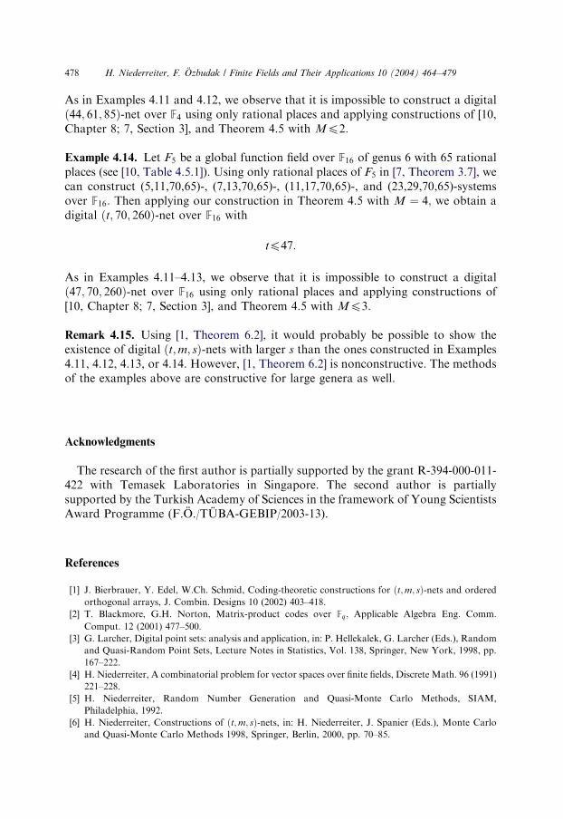
As in Examples 4.11 and 4.12, we observe that it is impossible to construct a digitalð44; 61; 85Þ-net over F4 using only rational places and applying constructions of [10,Chapter 8; 7, Section 3], and Theorem 4.5 with Mp2:
Example 4.14. Let F5 be a global function field over F16 of genus 6 with 65 rationalplaces (see [10, Table 4.5.1]). Using only rational places of F5 in [7, Theorem 3.7], wecan construct (5,11,70,65)-, (7,13,70,65)-, (11,17,70,65)-, and (23,29,70,65)-systemsover F16: Then applying our construction in Theorem 4.5 with M ¼ 4; we obtain adigital ðt; 70; 260Þ-net over F16 with
tp47:
As in Examples 4.11–4.13, we observe that it is impossible to construct a digitalð47; 70; 260Þ-net over F16 using only rational places and applying constructions of[10, Chapter 8; 7, Section 3], and Theorem 4.5 with Mp3:
Remark 4.15. Using [1, Theorem 6.2], it would probably be possible to show theexistence of digital ðt;m; sÞ-nets with larger s than the ones constructed in Examples4.11, 4.12, 4.13, or 4.14. However, [1, Theorem 6.2] is nonconstructive. The methodsof the examples above are constructive for large genera as well.
Acknowledgments
The research of the first author is partially supported by the grant R-394-000-011-422 with Temasek Laboratories in Singapore. The second author is partiallysupported by the Turkish Academy of Sciences in the framework of Young ScientistsAward Programme (F.O./TUBA-GEBIP/2003-13).
References
[1] J. Bierbrauer, Y. Edel, W.Ch. Schmid, Coding-theoretic constructions for ðt;m; sÞ-nets and ordered
orthogonal arrays, J. Combin. Designs 10 (2002) 403–418.
[2] T. Blackmore, G.H. Norton, Matrix-product codes over Fq; Applicable Algebra Eng. Comm.
Comput. 12 (2001) 477–500.
[3] G. Larcher, Digital point sets: analysis and application, in: P. Hellekalek, G. Larcher (Eds.), Random
and Quasi-Random Point Sets, Lecture Notes in Statistics, Vol. 138, Springer, New York, 1998, pp.
167–222.
[4] H. Niederreiter, A combinatorial problem for vector spaces over finite fields, Discrete Math. 96 (1991)
221–228.
[5] H. Niederreiter, Random Number Generation and Quasi-Monte Carlo Methods, SIAM,
Philadelphia, 1992.
[6] H. Niederreiter, Constructions of ðt;m; sÞ-nets, in: H. Niederreiter, J. Spanier (Eds.), Monte Carlo
and Quasi-Monte Carlo Methods 1998, Springer, Berlin, 2000, pp. 70–85.
ARTICLE IN PRESS
H. Niederreiter, F. .Ozbudak / Finite Fields and Their Applications 10 (2004) 464–479478
[7] H. Niederreiter, F. Ozbudak, Constructions of digital nets using global function fields, Acta Arith.
105 (2002) 279–302.
[8] H. Niederreiter, G. Pirsic, Duality for digital nets and its applications, Acta Arith. 97 (2001) 173–182.
[9] H. Niederreiter, G. Pirsic, A Kronecker product construction for digital nets, in: K.-T. Fang, F.J.
Hickernell, H. Niederreiter (Eds.), Monte Carlo and Quasi-Monte Carlo Methods 2000, Springer,
Berlin, 2002, pp. 396–405.
[10] H. Niederreiter, C.P. Xing, Rational Points on Curves over Finite Fields: Theory and Applications,
Cambridge University Press, Cambridge, 2001.
[11] G. van der Geer, M. van der Vlugt, Tables of curves with many points, available at http://
www.science.uva.nl/~geer/tables-mathcomp13.ps.
ARTICLE IN PRESS
H. Niederreiter, F. .Ozbudak / Finite Fields and Their Applications 10 (2004) 464–479 479