Embed Size (px)
Citation preview
Matrix Nearness Problems and Applications∗
Nicholas J. Higham†
Abstract
A matrix nearness problem consists of finding, for an arbitrary matrix A, a
nearest member of some given class of matrices, where distance is measured in a
matrix norm. A survey of nearness problems is given, with particular emphasis
on the fundamental properties of symmetry, positive definiteness, orthogonality,
normality, rank-deficiency and instability. Theoretical results and computational
methods are described. Applications of nearness problems in areas including control
theory, numerical analysis and statistics are outlined.
Key words. matrix nearness problem, matrix approximation, symmetry,
positive definiteness, orthogonality, normality, rank-deficiency, instability.
AMS subject classifications. Primary 65F30, 15A57.
1 Introduction
Consider the distance function
(1.1) d(A) = min{‖E‖ : A + E ∈ S has property P
}, A ∈ S,
where S denotes Cm×n or R
m×n, ‖ · ‖ is a matrix norm on S, and P is a matrix property
which defines a subspace or compact subset of S (so that d(A) is well-defined). Associated
with (1.1) are the following tasks, which we describe collectively as a matrix nearness
problem:
• Determine an explicit formula for d(A), or a useful characterisation.
∗This is a reprint of the paper: N. J. Higham. Matrix nearness problems and applications. In M. J. C.
Gover and S. Barnett, editors, Applications of Matrix Theory, pages 1–27. Oxford University Press, 1989.†Department of Mathematics, University of Manchester, Manchester, M13 9PL, England
1
• Determine X = A + Emin, where Emin is a matrix for which the minimum in (1.1)
is attained. Is X unique?
• Develop efficient algorithms for computing or estimating d(A) and X.
Matrix nearness problems arise in many areas of applied matrix computations. A
common situation is where a matrix A approximates a matrix B, and B is known to
possess a property P . Because of rounding errors or truncation errors incurred when
evaluating A, A does not have property P . An intuitively appealing way of “improving”
A is to replace it by a nearest matrix X with property P . A trivial example is where
computations with a real matrix move temporarily into the complex domain, and round-
ing errors force a result with nonzero imaginary part (this can happen, for example, when
computing a matrix function via an eigendecomposition); here one would simply take the
real part of the answer.
Conversely, in some applications it is important that A does not have a certain prop-
erty P , and it useful to know how close A is to having the undesirable property. If d(A)
is small then the source problem is likely to be ill-conditioned for A, and remedial action
may need to be taken. Nearness problems arising in this context involve, for example,
the properties of singularity and instability.
The choice of norm in (1.1) is usually guided by the tractability of the nearness
problem. The two most useful norms are the Frobenius (or Euclidean) norm
‖A‖F =(∑
i,j
|aij|2)1/2
= trace(A∗A)1/2,
and the 2-norm
‖A‖2 = ρ(A∗A
)1/2,
where A ∈ Cm×n, ρ is the spectral radius, and ∗ denotes the conjugate transpose. Both
norms are unitarily invariant, that is, ‖UAV ‖ = ‖A‖ for any unitary U and V . Moreover,
the Frobenius norm is strictly convex and is a differentiable function of the matrix ele-
ments. As we shall see, nearest matrices X are often unique in the Frobenius norm, but
not so in the 2-norm. Since ‖A‖2 ≤ ‖A‖F, with equality if A has rank one, it holds that
d2(A) ≤ dF (A), with equality if Emin for the 2-norm has rank one; this latter property
holds for several nearness problems. We will not consider the 1- and ∞-norms since they
generally lead to intractable nearness problems.
In computing d(A) it is important to understand the limitations imposed by finite-
precision arithmetic. The following perturbation result is useful in this regard:
(1.2) |d(A + ∆A) − d(A)| ≤ ‖∆A‖ =: ǫ‖A‖.
2
In floating point arithmetic with unit roundoff u, A may be contaminated by rounding
errors of order u‖A‖, and so from (1.2) we must accept uncertainty in d(A) also of order
u‖A‖. It is instructive to write (1.2) in the form
|d(A + ∆A) − d(A)|/‖A‖d(A)/‖A‖ ≤ ǫ
d(A)/‖A‖ ,
which shows that the smaller the relative distance d(A)/‖A‖, the larger the bound on the
relative accuracy with which it can be computed (this is analogous to results of the form
“the condition number of the condition number is the condition number”—see Demmel
(1987b)).
Several nearness problems have the pleasing feature that their solutions can be ex-
pressed in terms of matrix decompositions. Three well-known decompositions which will
be needed are the following:
Hermitian/Skew-Hermitian Parts
Any A ∈ Cn×n may be expressed in the form
A = 12(A + A∗) + 1
2(A − A∗) ≡ AH + AK .
AH is called the Hermitian part of A and AK the skew-Hermitian part.
Polar Decomposition
For A ∈ Cm×n, m ≥ n, there exists a matrix U ∈ C
m×n with orthonormal columns,
and a unique Hermitian positive semi-definite matrix H ∈ Cn×n, such that A = UH.
Singular Value Decomposition (SVD)
For A ∈ Cm×n, m ≥ n, there exist unitary matrices U ∈ C
m×m and V ∈ Cn×n such
that
(1.3)A = U
[Σ
0
]V ∗,
Σ = diag(σi), σ1 ≥ σ2 ≥ · · · ≥ σn ≥ 0.
The central role of the SVD in matrix nearness problems was first identified by Golub
(1968), who gives an early description of what is now the standard algorithm for com-
puting the SVD.
The analytic techniques needed to solve nearness problems are various. Some general
techniques are described and illustrated in Keller (1975). Every problem solver’s toolbox
should contain a selection of eigenvalue and singular value inequalities; excellent refer-
ences for these are Wilkinson (1965), Rao (1980) and Golub and Van Loan (1983). Also
of potential use is a general result of Lau and Riha (1981) which characterises, in the
2-norm, best approximations to an element of Rn×n by elements of a linear subspace. We
3
note, however, that the matrix properties P of interest in (1.1) usually do not define a
subspace.
In sections 2–7 we survey in detail nearness problems and applications involving the
properties of symmetry, positive semi-definiteness, orthogonality, normality, rank defi-
ciency and instability. Some other nearness problems are discussed briefly in the final
section.
Since most applications involve real matrices we will take the set S in (1.1) to be
Rm×n except for those properties (normality and instability) where, when S = C
m×n,
Emin may be complex even when A is real.
2 Symmetry
For A ∈ Rn×n let
η(A) = min{‖E‖ : A + E ∈ R
n×n is symmetric}.
Fan and Hoffman (1955) solved this nearness to symmetry problem for the unitarily
invariant norms, obtaining
η(A) = ‖AK‖ = 12‖A − AT‖, X = AH = 1
2(A + AT ).
Their proof is simple. For any symmetric Y ,
‖A − AH‖ = ‖AK‖ = 12‖(A − Y ) + (Y T − AT )‖
≤ 12‖A − Y ‖ + 1
2‖(Y − A)T‖
= ‖A − Y ‖,
using the fact that ‖A‖ = ‖AT‖ for any unitarily invariant norm.
For the Frobenius norm X is unique: this is a consequence of the strict convexity of
the norm. It is easy to see that X need not be unique in the 2-norm.
An important application of the nearest symmetric matrix problem occurs in optimisa-
tion when approximating the Hessian matrix(
∂2F∂xi∂xj
)of F : R
n → R by finite differences
of the gradient vector(
∂F∂xi
). The Hessian is symmetric but a difference approximation A
is usually not, and it is standard practice to approximate the Hessian by AH instead of
A (Gill, Murray and Wright 1981, p. 116; Dennis and Schnabel 1983, p. 103).
Entirely analogous to the above is the nearest skew-symmetric matrix problem; the
solution is X = AK for any unitarily invariant norm.
4
3 Positive Semi-Definiteness
For A ∈ Rn×n let
δ(A) = min{‖E‖ : E ∈ R
n×n, A + E = (A + E)T ≥ 0},
where Y ≥ 0 denotes that the symmetric matrix Y is positive semi-definite (psd), that
is, it’s eigenvalues are nonnegative. Any psd X satisfying ‖A − X‖ = δ(A) is termed a
positive approximant of A.
The positive approximation problem has been solved in both the Frobenius norm and
the 2-norm. Let λi(A) denote an eigenvalue of A.
Theorem 3.1. (Higham 1988a) Let A ∈ Rn×n and let AH = UH be a polar de-
composition. Then XF = (AH + H)/2 is the unique positive approximant of A in the
Frobenius norm, and
δF (A)2 =∑
λi(AH)<0
λi(AH)2 + ‖AK‖2F.
Theorem 3.2. (Halmos 1972) For A ∈ Rn×n
δ2(A) = min{r ≥ 0 : r2I + A2
K ≥ 0 and G(r) ≥ 0},
where
(3.1) G(r) = AH + (r2I + A2K)1/2.
The matrix P = G(δ2(A)
)is a 2-norm positive approximant of A.
To prove Theorem 3.1 one shows that a positive approximant of A is a positive
approximant of AH , and that the latter is obtained by adding a perturbation which
shifts all negative eigenvalues of AH to the origin. The proof of Theorem 3.2 is more
complicated. Halmos actually proves the result in the more general context of linear
operators on a Hilbert space.
The 2-norm and Frobenius norm positive approximation problems can be related as
follows. First, if A is normal (see section 5) then XF is a 2-norm positive approximant
of A (Halmos 1972). Second, XF is always an approximate minimiser of the 2-norm
distance ‖A − X‖2, since (Higham 1988a)
δ2(A) ≤ ‖A − XF‖2 ≤ 2δ2(A).
5
Computation of the (unique) Frobenius norm positive approximant is straightforward.
Any method for computing the polar decomposition may be used (see section 4) to
obtain AH = UH and thence XF . Since AH is symmetric the preferred approach is to
compute a spectral decomposition AH = Z diag(λi)ZT (ZT Z = I), in terms of which
XF = Z diag(di)ZT , where di = max(λi, 0).
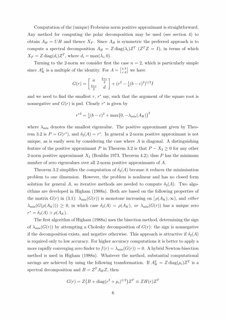
Turning to the 2-norm we consider first the case n = 2, which is particularly simple
since A2K is a multiple of the identity. For A =
[ac
bd
]we have
G(r) =
[a b+c
2b+c2
d
]+ (r2 − 1
4(b − c)2)1/2I
and we need to find the smallest r, r∗ say, such that the argument of the square root is
nonnegative and G(r) is psd. Clearly r∗ is given by
r∗2 = 14(b − c)2 + max
(0,−λmin(AH)
)2
where λmin denotes the smallest eigenvalue. The positive approximant given by Theo-
rem 3.2 is P = G(r∗), and δ2(A) = r∗. In general a 2-norm positive approximant is not
unique, as is easily seen by considering the case where A is diagonal. A distinguishing
feature of the positive approximant P in Theorem 3.2 is that P − X2 ≥ 0 for any other
2-norm positive approximant X2 (Bouldin 1973, Theorem 4.2); thus P has the minimum
number of zero eigenvalues over all 2-norm positive approximants of A.
Theorem 3.2 simplifies the computation of δ2(A) because it reduces the minimisation
problem to one dimension. However, the problem is nonlinear and has no closed form
solution for general A, so iterative methods are needed to compute δ2(A). Two algo-
rithms are developed in Higham (1988a). Both are based on the following properties of
the matrix G(r) in (3.1): λmin(G(r)) is monotone increasing on [ ρ(AK),∞), and either
λmin(G(ρ(AK))) ≥ 0, in which case δ2(A) = ρ(AK), or λmin(G(r)) has a unique zero
r∗ = δ2(A) > ρ(AK).
The first algorithm of Higham (1988a) uses the bisection method, determining the sign
of λmin(G(r)) by attempting a Cholesky decomposition of G(r): the sign is nonnegative
if the decomposition exists, and negative otherwise. This approach is attractive if δ2(A)
is required only to low accuracy. For higher accuracy computations it is better to apply a
more rapidly converging zero finder to f(r) = λmin(G(r)) = 0. A hybrid Newton-bisection
method is used in Higham (1988a). Whatever the method, substantial computational
savings are achieved by using the following transformation. If A2K = Z diag(µi)Z
T is a
spectral decomposition and B = ZT AHZ, then
G(r) = Z(B + diag(r2 + µi)
1/2)ZT ≡ ZH(r)ZT
6
where repeated evaluations of H(r) for different r are inexpensive, and f(r) = λmin(H(r)).
Furthermore, good initial bounds for δ2(A), differing by no more than a factor of two,
are provided by
max{ρ(AK), max
bii<0
(b2ii − µi
)1/2, M
}≤ δ2(A) ≤ ρ(AK) + M,
where M = max(0,−λmin(AH)
)(Higham 1988a).
Our experience is that the Newton-bisection algorithm performs well even when
G(δ2(A)) has multiple zero eigenvalues, in which case f(r) is not differentiable at r∗ =
δ2(A). The only drawback of Halmos’ formula for δ2(A) is a potential for losing signif-
icant figures when forming G(r), but fortunately such loss of significance is relatively
uncommon (see Higham (1988a)).
The most well-known application of the positive approximation problem is in detecting
and modifying an indefinite Hessian matrix in Newton methods for optimisation (Gill,
Murray and Wright 1981, sec. 4.4.2). Two other applications involving sparse matrices
are discussed in Duff, Erisman and Reid (1986, sec. 12.5).
4 Orthogonality
In this section we consider finding a nearest matrix with orthonormal columns to A ∈R
m×n (m ≥ n), and its distance from A
(4.1) γ(A) = min{‖E‖ : E ∈ R
m×n, (A + E)T (A + E) = I}.
A related problem is the orthogonal Procrustes problem: given A,B ∈ Rm×n find
(4.2) min{‖A − BQ‖F : Q ∈ R
n×n, QT Q = I}.
This requires us to find an orthogonal matrix which most nearly transforms B into A in
a least squares sense. Solutions to these problems are given in the following theorem.
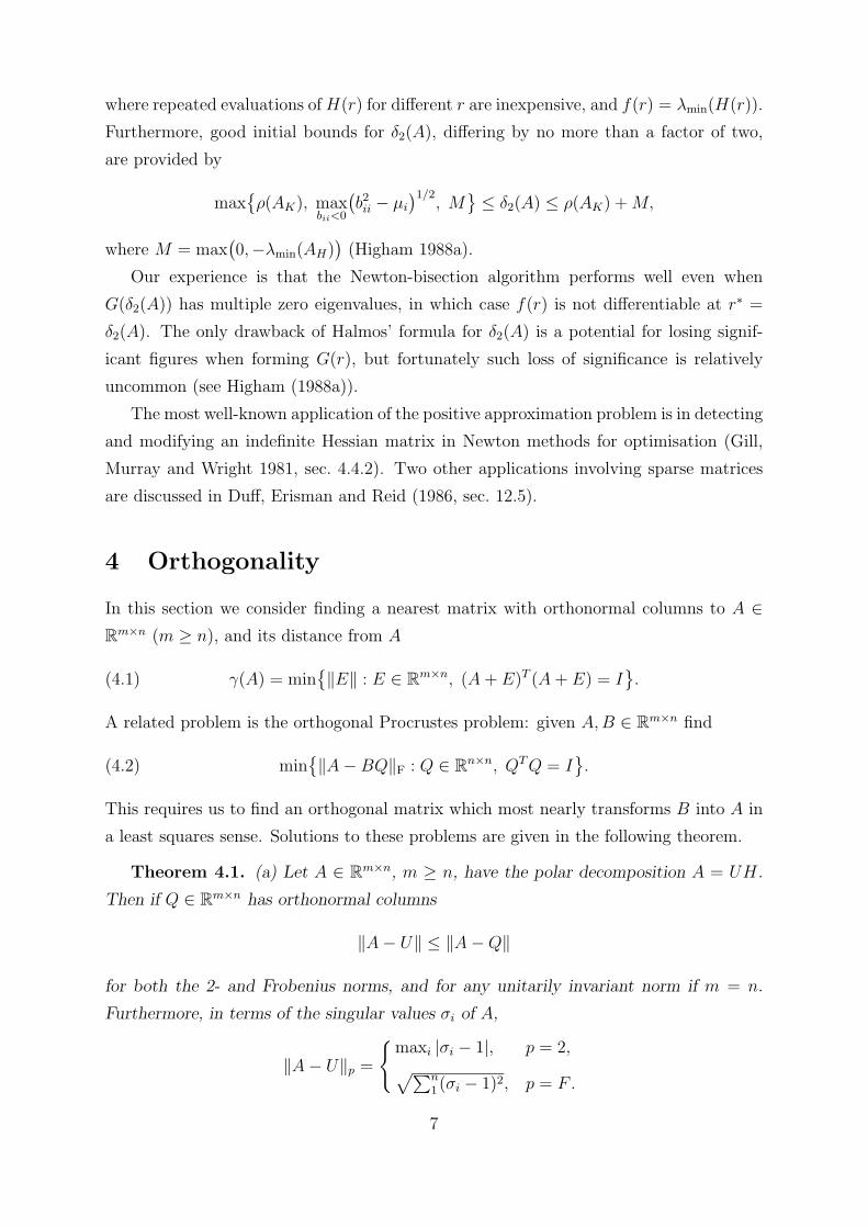
Theorem 4.1. (a) Let A ∈ Rm×n, m ≥ n, have the polar decomposition A = UH.
Then if Q ∈ Rm×n has orthonormal columns
‖A − U‖ ≤ ‖A − Q‖
for both the 2- and Frobenius norms, and for any unitarily invariant norm if m = n.
Furthermore, in terms of the singular values σi of A,
‖A − U‖p =
{maxi |σi − 1|, p = 2,√∑n
1 (σi − 1)2, p = F .
7
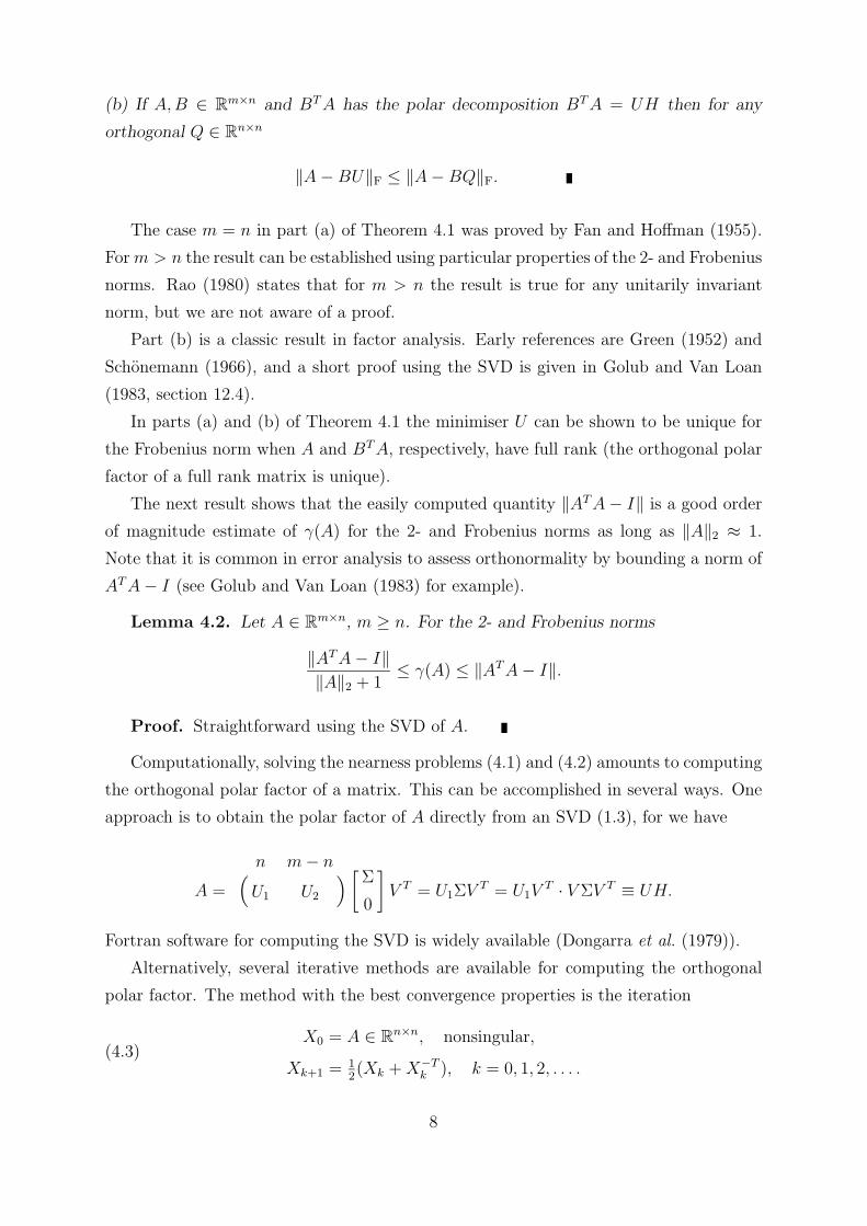
(b) If A,B ∈ Rm×n and BT A has the polar decomposition BT A = UH then for any
orthogonal Q ∈ Rn×n
‖A − BU‖F ≤ ‖A − BQ‖F.
The case m = n in part (a) of Theorem 4.1 was proved by Fan and Hoffman (1955).
For m > n the result can be established using particular properties of the 2- and Frobenius
norms. Rao (1980) states that for m > n the result is true for any unitarily invariant
norm, but we are not aware of a proof.
Part (b) is a classic result in factor analysis. Early references are Green (1952) and
Schonemann (1966), and a short proof using the SVD is given in Golub and Van Loan
(1983, section 12.4).
In parts (a) and (b) of Theorem 4.1 the minimiser U can be shown to be unique for
the Frobenius norm when A and BT A, respectively, have full rank (the orthogonal polar
factor of a full rank matrix is unique).
The next result shows that the easily computed quantity ‖AT A − I‖ is a good order
of magnitude estimate of γ(A) for the 2- and Frobenius norms as long as ‖A‖2 ≈ 1.
Note that it is common in error analysis to assess orthonormality by bounding a norm of
AT A − I (see Golub and Van Loan (1983) for example).
Lemma 4.2. Let A ∈ Rm×n, m ≥ n. For the 2- and Frobenius norms
‖AT A − I‖‖A‖2 + 1
≤ γ(A) ≤ ‖AT A − I‖.
Proof. Straightforward using the SVD of A.
Computationally, solving the nearness problems (4.1) and (4.2) amounts to computing
the orthogonal polar factor of a matrix. This can be accomplished in several ways. One
approach is to obtain the polar factor of A directly from an SVD (1.3), for we have
A =( n m − n
U1 U2
) [Σ
0
]V T = U1ΣV T = U1V
T · V ΣV T ≡ UH.
Fortran software for computing the SVD is widely available (Dongarra et al. (1979)).
Alternatively, several iterative methods are available for computing the orthogonal
polar factor. The method with the best convergence properties is the iteration
(4.3)X0 = A ∈ R
n×n, nonsingular,
Xk+1 = 12(Xk + X−T
k ), k = 0, 1, 2, . . . .
8
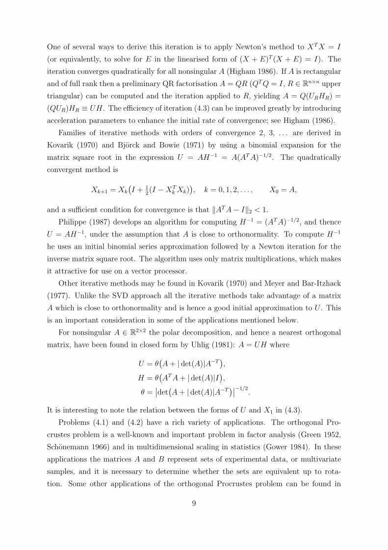
One of several ways to derive this iteration is to apply Newton’s method to XT X = I
(or equivalently, to solve for E in the linearised form of (X + E)T (X + E) = I). The
iteration converges quadratically for all nonsingular A (Higham 1986). If A is rectangular
and of full rank then a preliminary QR factorisation A = QR (QT Q = I, R ∈ Rn×n upper
triangular) can be computed and the iteration applied to R, yielding A = Q(URHR) =
(QUR)HR ≡ UH. The efficiency of iteration (4.3) can be improved greatly by introducing
acceleration parameters to enhance the initial rate of convergence; see Higham (1986).
Families of iterative methods with orders of convergence 2, 3, . . . are derived in
Kovarik (1970) and Bjorck and Bowie (1971) by using a binomial expansion for the
matrix square root in the expression U = AH−1 = A(AT A)−1/2. The quadratically
convergent method is
Xk+1 = Xk
(I + 1
2(I − XT
k Xk)), k = 0, 1, 2, . . . , X0 = A,
and a sufficient condition for convergence is that ‖AT A − I‖2 < 1.
Philippe (1987) develops an algorithm for computing H−1 = (AT A)−1/2, and thence
U = AH−1, under the assumption that A is close to orthonormality. To compute H−1
he uses an initial binomial series approximation followed by a Newton iteration for the
inverse matrix square root. The algorithm uses only matrix multiplications, which makes
it attractive for use on a vector processor.
Other iterative methods may be found in Kovarik (1970) and Meyer and Bar-Itzhack
(1977). Unlike the SVD approach all the iterative methods take advantage of a matrix
A which is close to orthonormality and is hence a good initial approximation to U . This
is an important consideration in some of the applications mentioned below.
For nonsingular A ∈ R2×2 the polar decomposition, and hence a nearest orthogonal
matrix, have been found in closed form by Uhlig (1981): A = UH where
U = θ(A + | det(A)|A−T
),
H = θ(AT A + | det(A)|I
),
θ =∣∣det
(A + | det(A)|A−T
)∣∣−1/2.
It is interesting to note the relation between the forms of U and X1 in (4.3).
Problems (4.1) and (4.2) have a rich variety of applications. The orthogonal Pro-
crustes problem is a well-known and important problem in factor analysis (Green 1952,
Schonemann 1966) and in multidimensional scaling in statistics (Gower 1984). In these
applications the matrices A and B represent sets of experimental data, or multivariate
samples, and it is necessary to determine whether the sets are equivalent up to rota-
tion. Some other applications of the orthogonal Procrustes problem can be found in
9
Brock (1968), Lefkovitch (1978), Wahba (1965) and Hanson and Norris (1981) (in the
latter two references the additional constraint det(Q) = 1 is imposed).
In aerospace computations a 3×3 orthogonal matrix called the direction cosine matrix
(DCM) transforms vectors between one coordinate system and another. The DCM is
defined as the solution to a matrix differential equation; approximate solutions of the
differential equation usually drift from orthogonality, and so periodic re-orthogonalisation
is necessary. A popular way to achieve this is to replace a DCM approximation by
the nearest orthogonal matrix. See Bjorck and Bowie (1971), Meyer and Bar-Itzhack
(1977), and the references therein. Similarly, one way to improve the orthonormality of
a set of computed eigenvectors of a symmetric matrix (obtained by inverse iteration, for
example) is to replace them by a nearest orthonormal set of vectors. Advantages claimed
over Gram-Schmidt or QR orthonormalisation are the intrinsic minimum perturbation
property, and the fact that the nearest orthonormal matrix is essentially independent
of the column ordering (since A = UH implies AP = UP · P T HP ≡ U ′H ′ for any
permutation matrix P , that is, the nearest orthonormal matrix is permuted in the same
way as A).
5 Normality
A matrix A ∈ Cn×n is normal if A∗A = AA∗. There are many characterisations of
a normal matrix (seventy conditions which are equivalent to A∗A = AA∗ are listed in
Grone et al. (1987)!). The most fundamental characterisation is that A is normal if and
only if there exists a unitary matrix Z such that
Z∗AZ = diag(λi).
Thus the normal matrices are those with a complete set of orthonormal eigenvectors. Note
that the set of normal matrices includes the sets of Hermitian (λi real), skew-Hermitian
(λi imaginary) and unitary (|λi| = 1) matrices. Thus the quantity
ν(A) = min{‖E‖ : A + E ∈ C
n×n normal}
is no larger than the nearness measures considered in the previous sections, and because
of the generality of the normal matrices one might expect determination of a nearest
normal matrix to be particularly difficult. This is indeed the case, and the nearness to
normality problem has only recently been completely solved (in the Frobenius norm only),
by Gabriel (1979) (see also Gabriel (1987) and the references therein) and, independently,
by Ruhe (1987). This latter paper contains the most elegant and concise presentation,
and we follow it here.
10
An early and thorough treatment of the nearness to normality problem, containing a
partial solution, is given in the unpublished thesis of Causey (1964). The problem has also
received attention in the setting of a Hilbert space—references include Halmos (1974),
Holmes (1974) and Phillips (1977). Unfortunately, most of the results in these papers
are vacuous when applied to Cn×n.
The key to understanding and solving the nearness to normality problem in the Frobe-
nius norm is the following matrix decomposition introduced by Ruhe (1987). If A ∈ Cn×n
then
(5.1) A = D + H + S,
whereD = diag(akk), hkk ≡ 0, skk ≡ 0,
hjk =
{(ajk + exp(2iθjk)akj)/2, ajj 6= akk,
ajk, ajj = akk,(j 6= k)
sjk =
{(ajk − exp(2iθjk)akj)/2, ajj 6= akk,
0, ajj = akk,(j 6= k)
and where
θjk = arg(akk − ajj).
Note that if the diagonal elements of A are real and distinct then D + H ≡ AH and
S ≡ AK . Another interesting property is the Pythagorean relation ‖A‖2F = ‖D‖2
F +
‖H‖2F + ‖S‖2
F.
Ruhe shows that if N is the set of normal matrices then H may be regarded as being
tangential to N and S orthogonal to N, in the sense of the inner product (A,B) ≡ℜe trace(A∗B). Pursuing this geometric line of thought Ruhe notes that if X is a nearest
normal matrix to A then A−X must be orthogonal to N (cf. linear least squares theory).
In particular, for D, the diagonal part of A, to be a nearest normal matrix to A we need
H = 0. A matrix for which H = 0 in the DHS decomposition (5.1) is called a ∆H-matrix
(this term comes from Gabriel (1979)). Using the unitary invariance of the Frobenius
norm we have the following result. Here, diag(A) ≡ diag(aii).
Theorem 5.1. (Gabriel 1979, Theorem 3; Ruhe 1987) Let X be a nearest normal
matrix to A in the Frobenius norm, and let X = ZDZ∗ be a spectral decomposition.
Then Z∗AZ is a ∆H-matrix and D = diag(Z∗AZ).
Theorem 5.1 has two weaknesses: it is not constructive, and it gives a necessary but
not a sufficient condition for X to be a nearest normal matrix. However, an algorithm for
unitarily transforming an arbitrary A into a ∆H-matrix is readily available: the Jacobi
11
method for computing the eigensystem of a Hermitian matrix, as extended to normal
matrices by Goldstine and Horwitz (1959). Causey (1964) and Ruhe (1987) show that
when this algorithm is applied to a non-normal matrix it converges to a ∆H-matrix, and
both give a simplified description of the algorithm.
To obtain a sufficient condition for X to be a nearest normal matrix Ruhe examines
first and second order optimality conditions for the nonlinear optimisation problem
(5.2) minimise ‖A − X‖2F subject to X∗X − XX∗ = 0.
The Lagrangian function for (5.2) may be written
L(X,M) = trace((A − X)∗(A − X)
)− trace
(M∗(X∗X − XX∗)
),
where M is a Hermitian matrix of Lagrange multipliers whose diagonal is arbitrary. The
first order optimality condition, ∇XL(X,M) = 0, takes the form
X − A − XM + MX = 0.
If X is diagonal, one can show that this equation has a Hermitian solution M only if
A is a ∆H-matrix. This verifies Theorem 5.1. The second order necessary/sufficient
optimality condition turns out to be that
trace(H∗H − M∗H∗H + H∗HM∗)
is nonnegative/positive for all feasible perturbations H to X. Ruhe shows that this
condition can be expressed in terms of the definiteness of a certain real symmetric matrix
Gtang of order n2 + n. He also shows that the trace quantity is certainly positive if the
n2 × n2 Hermitian matrix
G = I − M ⊗ I + I ⊗ M
is positive definite, which is the case if
(5.3) spread(M) ≡ maxj
λj(M) − minj
λj(M) < 1.
This latter condition is easy to check, since it involves only an n × n matrix.
To summarise, the Jacobi algorithm transforms an arbitrary A into a ∆H-matrix:
Z∗AZ = D + S. (Note that in step 2 of Algorithm J in Ruhe (1987) “det” should be
“− det”.) X = ZDZ∗ is a putative nearest normal matrix. If (5.3) is satisfied then
X is optimal; otherwise, to determine optimality one must examine the definiteness of
Gtang. Ruhe (1987) found no examples where X was not a nearest normal matrix. The
drawbacks of Ruhe’s method are the linear convergence of the Jacobi algorithm in general,
and the expense of verifying optimality if Gtang has to be examined.
Some further insight into the nearest normal matrix is provided by the following
result.
12
Theorem 5.2. (Causey 1964, Theorem 5.13; Gabriel 1979, Theorem 1) Let A ∈ Cn×n
and let X = ZDZ∗, where Z is unitary and D is diagonal. Then X is a nearest normal
matrix to A in the Frobenius norm if and only if
(a) ‖ diag(Z∗AZ)‖F = maxQ∗Q=I
‖ diag(Q∗AQ)‖F, and
(b) D = diag(Z∗AZ).
The theorem has the pleasing interpretation that finding a nearest normal matrix is
equivalent to finding a unitary similarity transformation which makes the sum of squares
of the diagonal elements as large as possible. Much of the analysis in Causey (1964) is
based on this result; in particular, the Jacobi algorithm is derived from this perspective.
Also, a complete solution is developed for the case n = 2.
Theorem 5.3. (Causey 1964, Theorem 6.24) Let A ∈ C2×2 have eigenvalues λ1, λ2.
All nearest normal matrices to A in the Frobenius norm are given by
(5.4) X(µ) = 12(A + µA∗) +
1
4trace(A − µA∗)I, µ ∈ ζ(A),
where, with sign(z) = z/|z|,
ζ(A) =
{sign
((λ1 − λ2)
2), λ1 6= λ2,
{z ∈ C : |z| = 1}, λ1 = λ2.
The theorem confirms that a nearest normal matrix need not be unique in the Frobe-
nius norm, at least if there are repeated eigenvalues. It also shows that there can be a
non-real nearest normal matrix when A is real. If A is real one may well be interested
in a nearest real normal matrix. The following corollary of Theorem 5.3 describes the
n = 2 case.
Corollary 5.4. Let A ∈ R2×2 be non-normal, with eigenvalues λ1, λ2. If λ1 6= λ2
there is a unique nearest real normal matrix in the Frobenius norm, given by (5.4). If
λ1 = λ2 there are exactly two nearest real normal matrices in the Frobenius norm,
X = 12(A ± AT ) + 1
4trace(A ∓ AT )I.
It seems to be an open question whether there is always a real matrix amongst the
nearest normal matrices to a real A, and if so, how to compute one.
Finally we quote two easily computed bounds on ν(A):
‖A∗A − AA∗‖F
4‖A‖2
≤ νF (A) ≤(n3 − n
12
)1/4
‖A∗A − AA∗‖1/2F .
13
The upper bound, from Henrici (1962), is in fact an upper bound for Henrici’s “departure
from normality”(‖A‖2
F −n∑
j=1
|λj(A)|2)1/2
,
which is itself an upper bound for νF (A). The lower bound is proved by Elsner and
Paardekooper (1987). Unfortunately, the lower and upper bounds differ by orders of
magnitude when νF (A)/‖A‖F is small.
A nearest normal matrix is required in certain applications in control theory. Daniel
and Kouvaritakis (1983, 1984) suggest approximating a transfer function matrix by a
nearest normal matrix, the attraction being that the eigenvalues of a normal matrix
are well-conditioned with respect to perturbations in the matrix. These references are
concerned with the 2-norm; in the 1983 paper a nearest normal matrix is found in the
2 × 2 case.
6 Rank-Deficiency
Probably the oldest and most well-known nearness problem concerns nearest matrices of
lower rank. We consider first finding a nearest matrix with a given null vector x 6= 0:
(6.1) min{‖E‖ : (A + E)x = 0, E ∈ R
n×n}.
This problem can be solved for an arbitrary subordinate matrix norm using the following
result of Rigal and Gaches (1967): for B ∈ Rm×n
(6.2) min{‖B‖ : Bp = q
}=
‖q‖‖p‖ , Bmin = qzT ,
where z is a vector dual to p, that is,
zT p = ‖z‖D‖p‖ = 1 where ‖z‖D = maxx 6=0
|zT x|‖x‖ .
The minimum in (6.1) is therefore attained for the rank one matrix Emin = (−Ax)zT ,
where z is a vector dual to x, and ‖Emin‖ = ‖Ax‖/‖x‖. To find a nearest rank-deficient
matrix to A (assumed nonsingular) we simply minimise ‖Emin‖ over all nonzero x, ob-
taining ‖A−1‖−1. Thus
(6.3) min{‖E‖‖A‖ : A + E is singular
}= κ(A)−1,
where the condition number κ(A) = ‖A‖‖A−1‖, with equality for E = yzT , where
‖A−1y‖ = ‖A−1‖‖y‖ and z is dual to y. This result was proved by Kahan (1966),
who attributes it to Gastinel; a detailed discussion is given in Wilkinson (1986).
14
Next, we consider rectangular and possibly rank-deficient A. Let A ∈ Rm×n (m ≥ n)
have the SVD (1.3) and let k < r = rank(A). Then, for p = 2, F ,
(6.4) minrank(B)=k
‖A − B‖p = ‖A − Ak‖p =
σk+1, p = 2,√∑r
k+1 σ2i , p = F ,
where
(6.5) Ak = U
[Dk
0
]V T , Dk = diag(σ1, . . . , σk, 0, . . . , 0).
In the Frobenius norm Ak is a unique minimiser if σk > σk+1. This is a classical result,
proved for the Frobenius norm by Eckart and Young (1936). Mirsky (1960) showed that
Ak in (6.5) achieves the minimum in (6.4) for any unitarily invariant norm. (Alternative
references for proofs are Golub and Van Loan (1983, p. 19) for the 2-norm, Stewart
(1973, p. 322) for the Frobenius norm, and Rao (1980) for the unitarily invariant norms.)
The Eckart-Young result has many applications in statistics; see Gower (1984) for some
examples and further references.
Computing the distances and nearest matrices above is straightforward in principle,
although relatively expensive in many contexts. Therefore much research has been aimed
at estimating the quantities of interest. We refer the reader to Higham (1987) for a survey
of techniques for estimating κ(A) and a list of applications, and to Stewart (1984) and
Bjorck (1987) for details of rank computations for rectangular matrices and applications
to least squares problems.
The matrix Ak in (6.5) will, in general, differ from A in all its entries. In certain
applications this is unacceptable because submatrices of A may be fixed. For example
in statistics a regression matrix for a model with a constant term has a column of ones,
and this should not be perturbed. Several recent papers have shown how to extend (6.4)
to allow submatrices of A to be fixed. Golub et al. (1987) extend the Frobenius norm
result to allow for fixed columns, and discuss statistical applications. Demmel (1987c)
considers perturbations to A22 in the partitioning
(6.6) A =
[A11 A12
A21 A22
]∈ R
m×n.
He classifies the achievable ranks and finds minimal 2- and Frobenius norm perturbations
which achieve such ranks. Watson (1988a) extends Demmel’s results to a wider class
of norms. For the case where A is square and nonsingular Demmel (1988) introduces
a further level of generality by allowing 1, 2 or 3 of the submatrices in (6.6) to be
perturbed; for a wide class of norms he finds perturbations that induce singularity and
are within a small constant factor of having minimal norm. Watson (1988b) analyses the
corresponding problem for rectangular A.
15
7 Instability
A matrix A ∈ Cn×n is stable if all its eigenvalues have negative real part, and unstable
otherwise. Matrix stability is an important property in control and systems engineering.
One obvious measure of the stability of a matrix is its spectral abscissa
α(A) = maxj
ℜe λj(A).
However, as noted by Van Loan (1985), if A is stable −α(A) can be much larger than
the distance from A to the nearest unstable matrix,
(7.1) β(A) = min{‖E‖ : A + E ∈ C
n×n is unstable}.
For example, if A is the 5×5 upper triangular matrix with diagonal elements −0.1 and all
superdiagonal elements −1, then α(A) = −0.1, yet A is within 2-norm distance ≈ 10−5
of a singular, and hence unstable, matrix.
Some bounds on β(A) are provided by the following result, in which sep(A) is the
smallest singular value of the linear transformation Ψ(X) = AX + XA∗.
Theorem 7.1. (Van Loan 1985) If A ∈ Cn×n is stable, then for the 2- and Frobenius
norms,12sep(A) ≤ β(A) ≤ min
{−α(A), σmin(A), 1
2‖A + A∗‖
}.
Unfortunately, the upper and lower bounds in the theorem can differ by a large factor.
Van Loan therefore developed a characterisation useful for computing β(A) as follows.
First, note that by continuity of the eigenvalues a minimising perturbation E in (7.1)
will be such that A + E has a pure imaginary eigenvalue, that is, (A + E − µiI)z = 0
for some µ ∈ R and 0 6= z ∈ Cn×n. This means that (A − µiI) + E is singular, and
from (6.4) the minimum values of ‖E‖2 and ‖E‖F for any such E are both σmin(A−µiI)
(and, interestingly, E can be taken to be of rank one). To obtain the overall minimum
we minimise over all µ, to obtain
(7.2) β2(A) = βF (A) = minµ∈R
σmin(A − µiI).
It is clear from the derivation of (7.2) that in both norms a nearest unstable matrix
may be non-unique. Furthermore, if A is real all nearest unstable matrices may be non-
real. Van Loan (1985) shows that the distance to the nearest real unstable matrix can
be expressed as the solution to a constrained minimisation problem in Rn.
The analysis above simplifies the nearness to instability problem considerably, since
it reduces a minimisation over Cn×n to the minimisation over R of f(µ) = σmin(A− µiI)
16
(cf. the simplification afforded by Theorem 3.2). However, f is a nonlinear function
with up to n local minima, and it is a nontrivial task to compute the global minimum.
Van Loan suggests applying a one-dimensional “no-derivatives” minimiser, with function
values f(µ) approximated using a condition estimator in order to reduce the compu-
tational cost. Van Loan’s numerical experiments led him to conjecture that the local
minima of f occur at the imaginary parts of A’s eigenvalues, and he recommended the
approximation β2(A) ≈ minj f(ℑm λj(A)
).
Subsequently, Demmel (1987a) found a counter-example to Van Loan’s conjecture.
For n = 3 the example is, with b ≫ 1,
A =
−1 −b −b2
0 −1 −b
0 0 −1
, f(ℑm λj(A)
)≡ σmin(A) = O(b−1), β2(A) = O(b−2).
However, Demmel comments that unless A is close to being both defective and derogatory,
the heuristic is likely to give a reasonable approximation.
Byers (1988) has developed a bisection technique for computing β2(A) which is un-
troubled by the existence of local minima of f . His method hinges on the following result;
we give part of the proof since it is illuminating.
Theorem 7.2. (Byers 1988) If σ ≥ 0, then σ ≥ β2(A) if and only if the matrix
H(σ) =
[A −σI
σI −A∗
]∈ C
2n×2n
has an eigenvalue with zero real part.
Proof. If ωi is a pure imaginary eigenvalue of H(σ) then for some 0 6= z ∈ C2n,
H(σ)z = ωiz. Writing z = [ vT , uT ]T , we have (A − ωiI)v = σu and (A − ωiI)∗u = σv.
Thus σ is a singular value of A − ωiI, and hence σ ≥ β2(A) by (7.2). For a proof of the
“if” part see Byers (1988).
Byers’ algorithm starts with a bracket [a, b] containing β2(A), where a is some small
tolerance, and b is the upper bound from Theorem 7.1. It repeatedly refines the bracket
by choosing c ∈ (a, b) and using Theorem 7.2 to test whether β2(A) lies in [a, c] or [c, b].
Since the initial bracket can be very poor Byers uses exponent bisection (c =√
ab), rather
than standard bisection (c = (a + b)/2); the former is quicker at “getting on scale”.
The crucial step in the algorithm is testing whether the Hamiltonian matrix H(σ) has
a pure imaginary eigenvalue. Byers shows that if the eigenvalues of H(σ) are computed
using an algorithm that preserves Hamiltonian structure, then it is safe to test for an
eigenvalue with exactly zero real part: the correct decisions will be made except, possibly,
when |σ − β2(A)| ≈ ǫ‖A‖2 (cf. (1.2)), where ǫ depends on the unit roundoff and on the
17
eigenvalue algorithm. Software for Hamiltonian eigenvalue calculations is not widely
available and so it is natural to ask whether it is acceptable to use a standard eigenvalue
routine in Byers’ algorithm. The answer appears to be yes, provided that one regards
an eigenvalue as having zero real part if its computed real part has magnitude less than
a tolerance of order u1/2‖A‖F. The factor u1/2 stems from the property that the pure
imaginary eigenvalues of H(β2(A)) usually occur in 2 × 2 Jordan blocks (Byers, private
communication).
8 Other Nearness Problems
In this final section we describe briefly some further nearness problems, including several
of a different character to those considered so far.
It is easy to determine a nearest matrix to A ∈ Cn×n having a given eigenvalue λ,
since if λ is an eigenvalue of A+E then (A−λI)+E is singular and the problem reduces
to (6.3) (see Wilkinson (1986) for a full discussion, and also compare the derivation of
(7.2)). Finding a nearest matrix having a repeated eigenvalue (which may or may not be
specified) is a much more difficult problem; see Wilkinson (1984) and Demmel (1987b).
Many variations are possible on the orthogonal Procrustes problem (4.2). These
include allowing two-sided orthogonal transformations A−Q1BQ2 (see Rao (1980)), and
altering the constraint on Q in (4.2) to diag(QT Q) = I (see Gower (1984)). Gower (1984)
shows that (4.2) with Q restricted to being a permutation matrix can be phrased as a
linear programming problem. In Higham (1988b) a symmetric Procrustes problem is
described in which the constraint on Q in (4.2) is that of symmetry. This problem arises
in the determination of the symmetric strain matrix of an elastic structure, and it may
be solved using an SVD of A.
In metric scaling in statistics a symmetric matrix A ∈ Rn×n is called a distance matrix
if it has zero diagonal elements and nonpositive off-diagonal elements; and it is called a
Euclidean distance matrix if there exist vectors x1, x2, . . . , xn ∈ Rk (k ≤ n) such that
aij = −12‖xi − xj‖2
2 for all i, j. Mathar (1985) finds a nearest Euclidean distance matrix
to an arbitrary distance matrix. A special class of norms is used involving a projection
matrix.
Byers (1988) adapts his bisection technique for computing β2(A) (see section 7) to
the problem of finding a nearest matrix with an eigenvalue of modulus unity.
When solving a linear system Ax = b one is interested in whether a computed solution
y solves a nearby system: for example, whether the particular backward error
(8.1) µ(y) = min{‖E‖ : (A + E)y = b
}
18
is relatively small. From (6.2) it follows that for any subordinate matrix norm µ(y) =
‖b − Ay‖/‖y‖, and Emin has rank one. For the 2- and Frobenius norms we have
µ(y) =‖r‖2
‖y‖2
, Emin =ryT
yT y,
where r = b − Ay. If A is symmetric then it is natural to require that E be symmetric
and to define
(8.2) µS(y) = min{‖E‖ : (A + E)y = b, E = ET
}.
For the Frobenius norm there is the rank two solution
ESmin =
ryT + yrT
yT y− (rT y)yyT
(yT y)2,
and one can show that
µF (y) ≤ µSF (y) ≤
√2µF (y).
Thus, forcing the backward error matrix to be symmetric has little effect on its norm.
Problems (8.1) and (8.2) are well-known in the fields of nonlinear equations and
optimisation, where they arise in the derivation of Jacobian and Hessian updates for
quasi-Newton methods. Excellent references are Dennis and Schnabel (1979, 1983), which
also consider additional constraints in (8.2) such as positive definiteness and sparsity. In
(8.1) and (8.2) the minimisers are unique for the Frobenius norm, but in general are not
unique for the 2-norm (Dennis and Schnabel, 1983, p.191).
Finally, we note that in some contexts it is of interest to modify (1.1) to
d(A) = min{ǫ : |E| ≤ ǫ|A|, A + E ∈ S has property P
},
where |A| = (|aij|) and the matrix inequality is interpreted componentwise. Here we are
restricting the class of permissible perturbations, since aij = 0 implies eij = 0, and we
measure the size of E relative to A in a componentwise fashion. This componentwise
nearness problem is of interest in applications with structured A—for example where there
is sparsity. The problem has been solved for S = Cn×n and the property P specified in
(8.1) by Oettli and Prager (1964). There are plenty of open problems here for other
properties P (singularity, for example).
Acknowledgement
It is a pleasure to thank Professor G.H. Golub for stimulating my interest in nearness
problems, and for providing several of the references.
19
REFERENCES
Bjorck, A. (1987) Least Squares Methods, in Handbook of Numerical Analysis, Volume
1: Solution of Equations in Rn, Ciarlet, P.G. and Lions, J.L., eds., Elsevier/North
Holland, 1987.
Bjorck, A. and Bowie, C. (1971) An iterative algorithm for computing the best estimate
of an orthogonal matrix, SIAM J. Numer. Anal. 8, 358–364.
Bouldin, R. (1973) Positive approximants, Trans. Amer. Math. Soc. 177, 391–403.
Brock, J.E. (1968) Optimal matrices describing linear systems, AIAA Journal 6, 1292–
1296.
Byers, R. (1988) A bisection method for measuring the distance of a stable matrix to the
unstable matrices, SIAM J. Sci. Stat. Comput. 9, 875–881.
Causey, R.L. (1964) On Closest Normal Matrices, Ph.D. Thesis, Department of Computer
Science, Stanford University.
Daniel, R.W. and Kouvaritakis, B. (1983) The choice and use of normal matrix ap-
proximations to transfer-function matrices of multivariable control systems, Int. J.
Control 37, 1121–1133.
Daniel, R.W. and Kouvaritakis, B. (1984) Analysis and design of linear multivariable
feedback systems in the presence of additive perturbations, Int. J. Control 39, 551–
580.
Demmel, J.W. (1987a) A counterexample for two conjectures about stability, IEEE Trans.
Automat. Control AC-32, 340–342.
Demmel, J.W. (1987b) On condition numbers and the distance to the nearest ill-posed
problem, Numer. Math. 51, 251–289.
Demmel, J.W. (1987c) The smallest perturbation of a submatrix which lowers the rank
and constrained total least squares problems, SIAM J. Numer. Anal. 24, 199–206.
Demmel, J.W. (1988) On structured singular values, Manuscript, Computer Science De-
partment, Courant Institute of Mathematical Sciences, New York.
Dennis, J.E., Jr. and Schnabel, R.B. (1979) Least change secant updates for quasi-
Newton methods, SIAM Review 21, 443–459.
Dennis, J.E., Jr. and Schnabel, R.B. (1983) Numerical Methods for Unconstrained Op-
timization and Nonlinear Equations, Prentice-Hall, Englewood Cliffs, New Jersey.
Dongarra, J.J., Bunch, J.R., Moler, C.B. and Stewart, G.W. (1979) LINPACK Users’
Guide, Society for Industrial and Applied Mathematics, Philadelphia.
Duff, I.S., Erisman, A.M. and Reid, J.K. (1986) Direct Methods for Sparse Matrices,
Oxford University Press.
20
Eckart, C. and Young, G. (1936) The approximation of one matrix by another of lower
rank, Psychometrika 1, 211–218.
Elsner, L. and Paardekooper, M.H.C. (1987) On measures of nonnormality of matrices,
Linear Algebra and Appl. 92, 107–124.
Fan, K. and Hoffman, A.J. (1955) Some metric inequalities in the space of matrices, Proc.
Amer. Math. Soc. 6, 111–116.
Gabriel, R. (1979) Matrizen mit maximaler Diagonale bei unitarer Similaritat, J. Reine.
Angew. Math. 307/308, 31–52.
Gabriel, R. (1987) The normal ∆H-matrices with connection to some Jacobi-like meth-
ods, Linear Algebra and Appl. 91, 181–194.
Gill, P.E., Murray, W. and Wright, M.H. (1981) Practical Optimization, Academic Press,
London.
Goldstine, H.H. and Horwitz, L.P. (1959) A procedure for the diagonalization of normal
matrices, J. Assoc. Comput. Mach. 6, 176–195.
Golub, G.H. (1968) Least squares, singular values and matrix approximations, Aplikace
Matematiky 13, 44–51.
Golub, G.H., Hoffman, A. and Stewart, G.W. (1987) A generalization of the Eckart-
Young-Mirsky matrix approximation theorem, Linear Algebra and Appl. 88/89,
317–328.
Golub, G.H. and Van Loan, C.F. (1983) Matrix Computations, Johns Hopkins University
Press, Baltimore, Maryland.
Gower, J.C. (1984) Multivariate analysis: ordination, multidimensional scaling and allied
topics, in Handbook of Applicable Mathematics, Vol. VI: Statistics, Lloyd, E.H.,
ed., John Wiley, Chichester, 1984, pp. 727–781.
Green, B.F. (1952) The orthogonal approximation of an oblique structure in factor anal-
ysis, Psychometrika 17, 429–440.
Grone, R., Johnson, C.R., Sa, E.M. and Wolkowicz, H. (1987) Normal matrices, Linear
Algebra and Appl. 87, 213–225.
Halmos, P.R. (1972) Positive approximants of operators, Indiana Univ. Math. J. 21,
951–960.
Halmos, P.R. (1974) Spectral approximants of normal operators, Proc. Edinburgh Math.
Soc. 19, 51–58.
Hanson, R.J. and Norris, M.J. (1981) Analysis of measurements based on the singular
value decomposition, SIAM J. Sci. Stat. Comput. 2, 363–373.
Henrici, P. (1962) Bounds for iterates, inverses, spectral variation and fields of values of
non-normal matrices, Numer. Math. 4, 24–40.
21
Higham, N.J. (1986) Computing the polar decomposition—with applications, SIAM J.
Sci. Stat. Comput. 7, 1160–1174.
Higham, N.J. (1987) A survey of condition number estimation for triangular matrices,
SIAM Review 29, 575–596.
Higham, N.J. (1988a) Computing a nearest symmetric positive semidefinite matrix, Lin-
ear Algebra and Appl. 103, 103–118.
Higham, N.J. (1988b) The symmetric Procrustes problem, BIT 28, 133–143.
Holmes, R.B. (1974) Best approximation by normal operators, Journal of Approximation
Theory 12, 412–417.
Kahan, W. (1966) Numerical linear algebra, Canadian Math. Bulletin 9, 757–801.
Keller, J.B. (1975) Closest unitary, orthogonal and Hermitian operators to a given oper-
ator, Math. Mag. 48, 192–197.
Kovarik, Z. (1970) Some iterative methods for improving orthonormality, SIAM J. Numer.
Anal. 7, 386–389.
Lau, K.K. and Riha, W.O.J. (1981) Characterization of best approximations in normed
linear spaces of matrices by elements of finite-dimensional linear subspaces, Linear
Algebra and Appl. 35, 109–120.
Lefkovitch, L.P. (1978) Consensus coordinates from qualitative and quantitative at-
tributes, Biometrical J. 20, 679–691.
Mathar, R. (1985) The best Euclidian fit to a given distance matrix in prescribed dimen-
sions, Linear Algebra and Appl. 67, 1–6.
Meyer, J. and Bar-Itzhack, I.Y. (1977) Practical comparison of iterative matrix orthogo-
nalisation algorithms, IEEE Trans. Aerospace and Electronic Systems 13, 230–235.
Mirsky, L. (1960) Symmetric gauge functions and unitarily invariant norms, Quart. J.
Math. 11, 50–59.
Oettli, W. and Prager, W. (1964) Compatibility of approximate solution of linear equa-
tions with given error bounds for coefficients and right-hand sides, Numer. Math.
6, 405–409.
Philippe, B. (1987) An algorithm to improve nearly orthonormal sets of vectors on a
vector processor, SIAM J. Alg. Disc. Meth. 8, 396–403.
Phillips, J. (1977) Nearest normal approximation for certain operators, Proc. Amer.
Math. Soc. 67, 236–240.
Rao, C.R. (1980) Matrix approximations and reduction of dimensionality in multivari-
ate statistical analysis, in Multivariate Analysis-V, Krishnaiah, P.R., ed., North
Holland, Amsterdam, 1980, pp. 3–22.
22
Rigal, J.L. and Gaches, J. (1967) On the compatibility of a given solution with the data
of a linear system, J. Assoc. Comput. Mach. 14, 543–548.
Ruhe, A. (1987) Closest normal matrix finally found!, BIT 27, 585–598.
Schonemann, P.H. (1966) A generalized solution of the orthogonal Procrustes problem,
Psychometrika 31, 1–10.
Stewart, G.W. (1973) Introduction to Matrix Computations, Academic Press, New York.
Stewart, G.W. (1984) Rank degeneracy, SIAM J. Sci. Stat. Comput. 5, 403–413.
Uhlig, F. (1981) Explicit polar decomposition and a near-characteristic poynomial: the
2 × 2 case, Linear Algebra and Appl. 38, 239–249.
Van Loan, C.F. (1985) How near is a stable matrix to an unstable matrix?, in Linear
Algebra and its Role in Systems Theory, Datta, B.N., ed., Contemporary Math.,
Vol. 47, Amer. Math. Soc., 1985, pp. 465–478.
Wahba, G. (1965) Problem 65-1: A least squares estimate of satellite attitude, SIAM
Review 7, 409; solutions in vol. 8, 1966, 384-386.
Watson, G.A. (1988a) The smallest perturbation of a submatrix which lowers the rank
of the matrix; to appear in IMA Journal of Numerical Analysis.
Watson, G.A. (1988b) The smallest perturbations of submatrices for rank-deficiency,
Manuscript.
Wilkinson, J.H. (1965) The Algebraic Eigenvalue Problem, Oxford University Press.
Wilkinson, J.H. (1984) On neighbouring matrices with quadratic elementary divisors,
Numer. Math. 44, 1–21.
Wilkinson, J.H. (1986) Sensitivity of eigenvalues II, Utilitas Mathematica 30, 243–286.
23