Embed Size (px)
Citation preview

Chapter 8: Linear Algebraic Equations
• Matrix Methods for Linear Equations
• Uniqueness and Existence of Solutions
• Under-Determined Systems
• Over-Determined Systems
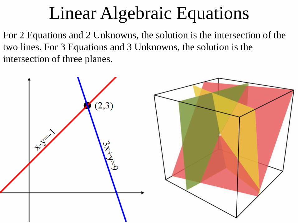
Linear Algebraic EquationsFor 2 Equations and 2 Unknowns, the solution is the intersection of the
two lines. For 3 Equations and 3 Unknowns, the solution is the
intersection of three planes.

Matrix Methods for Linear Systems of
Equations The simplest system of linear equations is:
𝑎𝑥 + 𝑏𝑦 = 𝑐𝑑𝑥 + 𝑒𝑦 = 𝑓
Two equations and two unknowns (all coefficients are known). Can be
solved by substitution, row reduction, Kramer’s Rule. Cast the system in
Vector Form:
𝑎 𝑏𝑑 𝑒
∙𝑥𝑦 =
𝑐𝑓
Matrix*Column Vector = Column Vector
𝐴 ∙ 𝑧 = 𝐵

Matrix Methods for Linear Systems of
Equations
𝐴 ∙ 𝑧 = 𝐵
Solve for solution vector 𝑧 by multiplying both sides by 𝐴−1 (𝐴 Inverse
[Matrix]):
𝐴−1 ∙ 𝐴 ∙ 𝑧 = 𝐴−1 ∙ (𝐵)
LHS: 𝐴−1 ∙ 𝐴 ∙ 𝑧 = 𝐴−1 ∙ 𝐴 ∙ 𝑧 = 𝐼 ∙ 𝑧 = 𝑧
𝐴−1 ∙ 𝐴 = 𝐼 Identity Matrix : 𝐼 =1 00 1
𝑧 = 𝐴−1 ∙ 𝐵where
𝐴−1 =1
𝑎𝑒 − 𝑏𝑑∙
𝑒 −𝑏−𝑑 𝑎
Matrix Methods for Linear Systems of
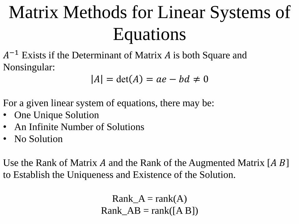
Equations 𝐴−1 Exists if the Determinant of Matrix 𝐴 is both Square and
Nonsingular:
𝐴 = det 𝐴 = 𝑎𝑒 − 𝑏𝑑 ≠ 0
For a given linear system of equations, there may be:
• One Unique Solution
• An Infinite Number of Solutions
• No Solution
Use the Rank of Matrix 𝐴 and the Rank of the Augmented Matrix [𝐴 𝐵]
to Establish the Uniqueness and Existence of the Solution.
Rank_A = rank(A)
Rank_AB = rank([A B])

Uniqueness and Existence of the
SolutionIf Rank_A ≠ Rank_AB, a Unique Solution Does Not Exist
If Rank_A = Rank_AB = Number of Unknowns, a Unique Solution
Exists
If Rank_A = Rank_AB but Rank_A ≠ Number of Unknowns, an Infinite
Number of Solutions Exist

Uniqueness and Existence of the
Solution% One Unique Solution: % x-y = -1, 3x+y = 9A = [1 -1; 3 1]B = [-1; 9]AB = [A B]rank_A = rank(A)rank_AB = rank(AB)Det_A = det(A)Inv_A = inv(A)z = Inv_A*B

Matrix Methods for Linear Systems of
Equations MATLAB has Several Methods of Solving Systems of Linear Equations:
• Matrix Inverse: z = inv(A)*B (Calculates the Inverse of 𝐴.)
• Left Division: z = A\B (Uses Gauss Elimination to Solve for 𝑧 for
Over-Determined Systems.)
• Pseudo-Inverse: z = pinv(A)*B (Used When There are More
Unknowns than Equations: Under-Determined Systems. This Method
Provides One Solution, but Not All Solutions.)
• Row-Reduced Echelon Form: rref([A B]) (Also Used for
Under-Determined Systems. This Method Provides a Set of Equations
That Can be Used to Find All Solutions.)

Under-Determined Systems Not Enough Information to Determine all of the Unknowns (Infinite
Number of Solutions)
Case 1: Fewer Equations than Unknowns:
𝑥 + 3𝑦 − 5𝑧 = 7−8𝑥 − 10𝑦 + 4𝑧 = 28
Case 2: Two Equations are Not Independent:
𝑥 + 3𝑦 − 5𝑧 = 7−8𝑥 − 10𝑦 + 4𝑧 = 28−16𝑥 − 20𝑦 + 8𝑧 = 56
(Equation 3) = 2*(Equation 2)
Solve Under-Determined Systems using Pseudo-Inverse pinv, which
finds one solution by minimizing the Euclidean Norm, or find all
possible solutions by using the rref method (Row-Reduced Echelon
Form).

Under-Determined Systems % Under-Determined System: % Inverse Method% x+3y-5z = 7, -8x-10y+4z = 28A = [1 3 -5; -8 -10 4]B = [7; 28]AB = [A B]rank_A = rank(A)rank_AB = rank(AB)Det_A = det(A)Inv_A = inv(A)z = Inv_A*B

Under-Determined Systems % Under-Determined System: % Pseudo-Inverse Method% x+3y-5z = 7, -8x-10y+4z = 28A = [1 3 -5; -8 -10 4]B = [7; 28]AB = [A B]rank_A = rank(A)rank_AB = rank(AB)z = pinv(A)*B

Row-Reduced Echelon Form𝑥 + 3𝑦 − 5𝑧 = 7
−8𝑥 − 10𝑦 + 4𝑧 = 28Replace (Equation 2) by 8*(Equation 1) + (Equation 2):
𝑥 + 3𝑦 − 5𝑧 = 70𝑥 + 14𝑦 − 36𝑧 = 84
Divide (Equation 2) by 14:
𝑥 + 3𝑦 − 5𝑧 = 7
0𝑥 + 𝑦 −36
14𝑧 = 6
Replace (Equation 1) by −3*(Equation 2) + (Equation 1):
𝑥 + 0𝑦 + 2.714𝑧 = −11
0𝑥 + 𝑦 −36
14𝑧 = 6
Infinite Number of Solutions because 𝑧 can be any number:
𝑥 + 2.714𝑧 = −11
𝑦 −36
14𝑧 = 6

Under-Determined Systems % Under-Determined System:% Row-Reduced Echelon Method% x+3y-5z = 7, -8x-10y+4z = 28A = [1 3 -5; -8 -10 4]B = [7; 28]AB = [A B]rank_A = rank(A)rank_AB = rank(AB)z = rref([A,B])
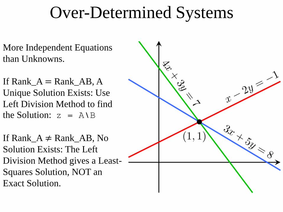
Over-Determined Systems
More Independent Equations
than Unknowns.
If Rank_A = Rank_AB, A
Unique Solution Exists: Use
Left Division Method to find
the Solution: z = A\B
If Rank_A ≠ Rank_AB, No
Solution Exists: The Left
Division Method gives a Least-
Squares Solution, NOT an
Exact Solution.

Over-Determined Systems % Over-Determined System:% 4x+3y = 7; x-2y = -1; 3x+5y = 8A = [4 3; 1 -2; 3 5]B = [7; -1; 8]AB = [A B]rank_A = rank(A)rank_AB = rank(AB)z = A\B

Over-Determined Systems % Over-Determined System:% 4x+3y = 6; x-2y = -1; 3x+5y = 8A = [4 3; 1 -2; 3 5]B = [6; -1; 8]AB = [A B]rank_A = rank(A)rank_AB = rank(AB)z = A\B

Problem 8.2:
𝐴 𝐵𝐶 + 𝐴 = 𝐵𝐴−1𝐴 𝐵𝐶 + 𝐴 = 𝐴−1𝐵
𝐵𝐶 + 𝐴 = 𝐴−1𝐵𝐵𝐶 = 𝐴−1𝐵 − 𝐴
𝐵−1𝐵𝐶 = 𝐵−1 𝐴−1𝐵 − 𝐴𝐶 = 𝐵−1 𝐴−1𝐵 − 𝐴

Problem 8.4:
a) Write a MATLAB script file that uses given values of the applied voltage 𝑣and the values of the five resistances and solves for the six currents.
b) Use the program developed in part a) to find the currents for the case where
𝑅1 = 1 kΩ, 𝑅2 = 5 kΩ, 𝑅3 = 2 kΩ, 𝑅4 = 10 kΩ, 𝑅5= 5 kΩ, and 𝑣 =100 𝑉 (1 kΩ = 1000 Ω).
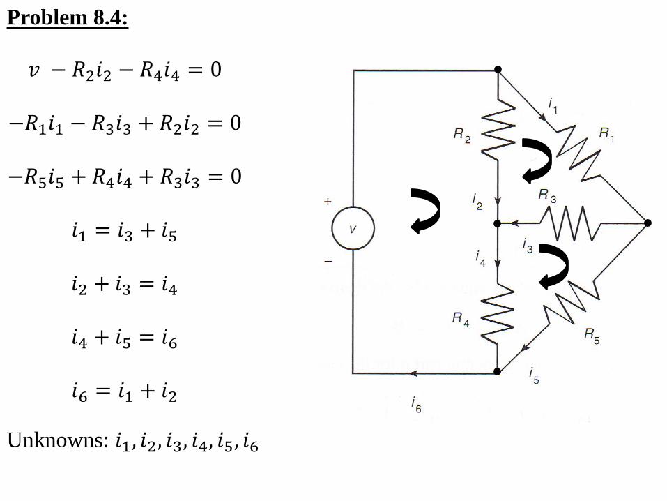
Problem 8.4:
Unknowns: 𝑖1, 𝑖2, 𝑖3, 𝑖4, 𝑖5, 𝑖6
𝑣 − 𝑅2𝑖2 − 𝑅4𝑖4 = 0
−𝑅1𝑖1 − 𝑅3𝑖3 + 𝑅2𝑖2 = 0
−𝑅5𝑖5 + 𝑅4𝑖4 + 𝑅3𝑖3 = 0
𝑖1 = 𝑖3 + 𝑖5
𝑖2 + 𝑖3 = 𝑖4
𝑖4 + 𝑖5 = 𝑖6
𝑖6 = 𝑖1 + 𝑖2
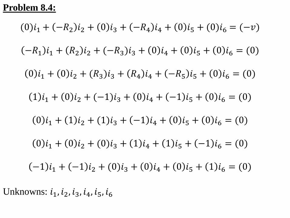
Problem 8.4:
Unknowns: 𝑖1, 𝑖2, 𝑖3, 𝑖4, 𝑖5, 𝑖6
(0)𝑖1+ −𝑅2 𝑖2 + 0 𝑖3 + −𝑅4 𝑖4 + 0 𝑖5 + (0)𝑖6 = (−𝑣)
−𝑅1 𝑖1 + 𝑅2 𝑖2 + (−𝑅3)𝑖3 + 0 𝑖4 + 0 𝑖5 + 0 𝑖6 = (0)
0 𝑖1 + 0 𝑖2 + (𝑅3)𝑖3 + 𝑅4 𝑖4 + −𝑅5 𝑖5 + 0 𝑖6 = (0)
1 𝑖1 + 0 𝑖2 + (−1)𝑖3 + 0 𝑖4 + −1 𝑖5 + 0 𝑖6 = (0)
0 𝑖1 + 1 𝑖2 + (1)𝑖3 + −1 𝑖4 + 0 𝑖5 + 0 𝑖6 = (0)
0 𝑖1 + 0 𝑖2 + (0)𝑖3 + 1 𝑖4 + 1 𝑖5 + −1 𝑖6 = (0)
−1 𝑖1 + −1 𝑖2 + (0)𝑖3 + 0 𝑖4 + 0 𝑖5 + 1 𝑖6 = (0)

Problem 8.4:

Problem 8.11:
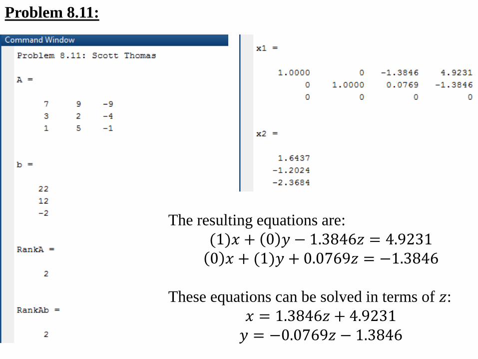
Problem 8.11:
The resulting equations are:
(1)𝑥 + 0 𝑦 − 1.3846𝑧 = 4.92310 𝑥 + (1)𝑦 + 0.0769𝑧 = −1.3846
These equations can be solved in terms of 𝑧:
𝑥 = 1.3846𝑧 + 4.9231𝑦 = −0.0769𝑧 − 1.3846

Problem 8.15: