Embed Size (px)
Citation preview
Matrix Factorization Techniques forTop-N Recommender Systems
Ernesto Diaz-Aviles<[email protected]>
Web Science 2013L3S Research Center. Hannover, Germany
Ernesto Diaz-Aviles <[email protected]> www.L3S.de | 1/39

Summary from Last Lecture
Learning to Rank
: Supervised Machine Learning Approach forRanking
Approaches : Pointwise, Pairwise, and Listwise Approaches.
Huge impact: Web Search, E-Business, Government, etc.
Ernesto Diaz-Aviles <[email protected]> www.L3S.de | 2/39

Summary from Last Lecture
Learning to Rank: Supervised Machine Learning Approach forRanking
Approaches : Pointwise, Pairwise, and Listwise Approaches.
Huge impact: Web Search, E-Business, Government, etc.
Ernesto Diaz-Aviles <[email protected]> www.L3S.de | 2/39

Summary from Last Lecture
Learning to Rank: Supervised Machine Learning Approach forRanking
Approaches
: Pointwise, Pairwise, and Listwise Approaches.
Huge impact: Web Search, E-Business, Government, etc.
Ernesto Diaz-Aviles <[email protected]> www.L3S.de | 2/39

Summary from Last Lecture
Learning to Rank: Supervised Machine Learning Approach forRanking
Approaches : Pointwise
, Pairwise, and Listwise Approaches.
Huge impact: Web Search, E-Business, Government, etc.
Ernesto Diaz-Aviles <[email protected]> www.L3S.de | 2/39

Summary from Last Lecture
Learning to Rank: Supervised Machine Learning Approach forRanking
Approaches : Pointwise, Pairwise
, and Listwise Approaches.
Huge impact: Web Search, E-Business, Government, etc.
Ernesto Diaz-Aviles <[email protected]> www.L3S.de | 2/39

Summary from Last Lecture
Learning to Rank: Supervised Machine Learning Approach forRanking
Approaches : Pointwise, Pairwise, and Listwise Approaches.
Huge impact: Web Search, E-Business, Government, etc.
Ernesto Diaz-Aviles <[email protected]> www.L3S.de | 2/39

Summary from Last Lecture
Learning to Rank: Supervised Machine Learning Approach forRanking
Approaches : Pointwise, Pairwise, and Listwise Approaches.
Huge impact: Web Search, E-Business, Government, etc.
Ernesto Diaz-Aviles <[email protected]> www.L3S.de | 2/39

Matrix Factorization Techniques forTop-N Recommender Systems
(Personalized Ranking)
Ernesto Diaz-Aviles <[email protected]> www.L3S.de | 4/39

Recommender Systems Tasks
1 Rating Prediction
2 Top-N Recommendation
Ernesto Diaz-Aviles <[email protected]> www.L3S.de | 6/39

Recommender Systems Tasks
1 Rating Prediction
2 Top-N Recommendation
Ernesto Diaz-Aviles <[email protected]> www.L3S.de | 6/39

Recommender Systems Tasks
1 Rating Prediction
2 Top-N Recommendation
(Item Prediction — Personalized Ranking)
Ernesto Diaz-Aviles <[email protected]> www.L3S.de | 7/39
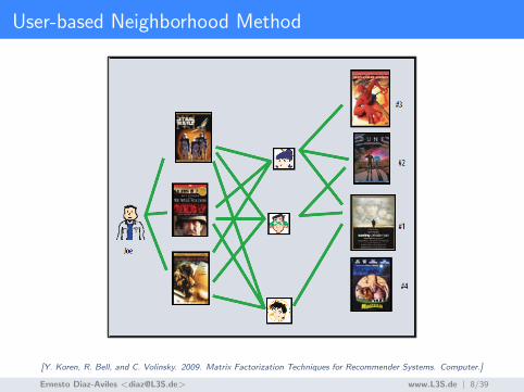
User-based Neighborhood Method
[Y. Koren, R. Bell, and C. Volinsky. 2009. Matrix Factorization Techniques for Recommender Systems. Computer.]
Ernesto Diaz-Aviles <[email protected]> www.L3S.de | 8/39

User-Item Matrix
User/Item I1 I2 I3 I4 I5 I6
U1 5 3 4
U2 1 1 1
U3 1 3 1
U4 5 2 2 5 4
U5 3 2
Ernesto Diaz-Aviles <[email protected]> www.L3S.de | 9/39

Matrix Factorization
Wi
Hj
Feedback Matrix: X = | U | x | i |
User Latent FactorsW = | U | x | k |
Item Latent FactorsH = | k | x | i |
Xij
Ernesto Diaz-Aviles <[email protected]> www.L3S.de | 10/39

MF and Latent FactorsCOVER FE ATURE
COMPUTER 44
vector qi ! f, and each user u is associ-ated with a vector pu ! f. For a given item i, the elements of qi measure the extent to which the item possesses those factors, positive or negative. For a given user u, the elements of pu measure the extent of interest the user has in items that are high on the corresponding factors, again, posi-tive or negative. The resulting dot product, qi
T pu, captures the interaction between user u and item i—the user’s overall interest in the item’s characteristics. This approximates user u’s rating of item i, which is denoted by rui, leading to the estimate
rui
= qiT pu. (1)
The major challenge is computing the map-ping of each item and user to factor vectors qi, pu ! f. After the recommender system completes this mapping, it can easily esti-mate the rating a user will give to any item by using Equation 1.
Such a model is closely related to singular value decom-position (SVD), a well-established technique for identifying latent semantic factors in information retrieval. Applying SVD in the collaborative filtering domain requires factoring the user-item rating matrix. This often raises difficulties due to the high portion of missing values caused by sparse-ness in the user-item ratings matrix. Conventional SVD is undefined when knowledge about the matrix is incom-plete. Moreover, carelessly addressing only the relatively few known entries is highly prone to overfitting.
Earlier systems relied on imputation to fill in missing ratings and make the rating matrix dense.2 However, im-putation can be very expensive as it significantly increases the amount of data. In addition, inaccurate imputation might distort the data considerably. Hence, more recent works3-6 suggested modeling directly the observed rat-ings only, while avoiding overfitting through a regularized model. To learn the factor vectors (pu and qi), the system minimizes the regularized squared error on the set of known ratings:
min* *,q p ( , )u i
(rui qiTpu)
2 + (|| qi ||2 + || pu ||
2) (2)
Here, is the set of the (u,i) pairs for which rui is known (the training set).
The system learns the model by fitting the previously observed ratings. However, the goal is to generalize those previous ratings in a way that predicts future, unknown ratings. Thus, the system should avoid overfitting the observed data by regularizing the learned parameters, whose magnitudes are penalized. The constant controls
recommendation. These methods have become popular in recent years by combining good scalability with predictive accuracy. In addition, they offer much flexibility for model-ing various real-life situations.
Recommender systems rely on different types of input data, which are often placed in a matrix with one dimension representing users and the other dimension representing items of interest. The most convenient data is high-quality explicit feedback, which includes explicit input by users regarding their interest in products. For example, Netflix collects star ratings for movies, and TiVo users indicate their preferences for TV shows by pressing thumbs-up and thumbs-down buttons. We refer to explicit user feedback as ratings. Usually, explicit feedback com-prises a sparse matrix, since any single user is likely to have rated only a small percentage of possible items.
One strength of matrix factorization is that it allows incorporation of additional information. When explicit feedback is not available, recommender systems can infer user preferences using implicit feedback, which indirectly reflects opinion by observing user behavior including pur-chase history, browsing history, search patterns, or even mouse movements. Implicit feedback usually denotes the presence or absence of an event, so it is typically repre-sented by a densely filled matrix.
A BASIC MATRIX FACTORIZATION MODEL Matrix factorization models map both users and items
to a joint latent factor space of dimensionality f, such that user-item interactions are modeled as inner products in that space. Accordingly, each item i is associated with a
Gearedtowardmales
Serious
Escapist
The PrincessDiaries
Braveheart
Lethal Weapon
IndependenceDay
Ocean’s 11Sense andSensibility
Gus
Dave
Gearedtoward
females
Amadeus
The Lion King Dumb andDumber
The Color Purple
Figure 2. A simpli!ed illustration of the latent factor approach, which characterizes both users and movies using two axes—male versus female and serious versus escapist. [Y. Koren, R. Bell, and C. Volinsky. 2009. Matrix Factorization Techniques for Recommender Systems. Computer.]
Ernesto Diaz-Aviles <[email protected]> www.L3S.de | 11/39

Matrix Factorization
Wi
Hj
Feedback Matrix: X = | U | x | i |
User Latent FactorsW = | U | x | k |
Item Latent FactorsH = | k | x | i |
Xij
Ernesto Diaz-Aviles <[email protected]> www.L3S.de | 12/39

CF Based on Matrix Factorization
MF estimates X : U × I by the product of two low-rankmatrices W : |U | × k and H : |I| × k as follows:
X := WHᵀ, where k is a parameter corresponding to therank of the approximation.
Ernesto Diaz-Aviles <[email protected]> www.L3S.de | 13/39

General Stochastic Gradient Descent Procedure for MF
SGD for MF
Input:Training data S; Regularization parameters λW and λH ;Learning rate η0; Learning rate schedule α; Number ofiterations T
Output: θ = (W,H)1: initialize W0 and H0
2: for t = 1 to T do3: (u, i, xui)← randomExample(S)4: wu ← wu − η ∂
∂wu`(xui, 〈wu,hi〉)− η λW wu
5: hi ← hi − η ∂∂hi
`(xui, 〈wu,hi〉)− η λH hi6: η = α · η7: end for8: return θT = (WT ,HT )
Ernesto Diaz-Aviles <[email protected]> www.L3S.de | 14/39

Learning Algorithms: Standard Framework†
Assumption: examples are drawn independently from anunknown probability distribution P (x, y) that represents therules of Nature
Expected Risk: E(f) =∫`(f(x), y) dP (x, y)
Empirical Risk: En(f) = 1n
∑n `(f(xi), yi)
We would like f∗ that minimizes E(f) among all functions
In general f∗ /∈ FThe best we can have is f∗F that minimizes E(f) inside FBut P (x, y) is unknown by definition
Instead we compute fn ∈ F that minimized En(f)
Vapnik-Chervonenkis theory tells us when this can work
†Leon Bottou: The Tradeoffs of Large Scale Learning, NIPS tutorials, Vancouver, 2007
Ernesto Diaz-Aviles <[email protected]> www.L3S.de | 16/39

Learning with Approximate Optimization†
Computing fn = argmin f ∈ FEn(f) is often costly
Since we already make lots of approximations, why should wecompute fn exactly?
Let’s assume our optimizer returns fn such thatEn(fn) < En(fn) + ε
For instance, one could stop an iterative optimizationalgorithm long before its convergence
†Leon Bottou: The Tradeoffs of Large Scale Learning, NIPS tutorials, Vancouver, 2007
Ernesto Diaz-Aviles <[email protected]> www.L3S.de | 17/39

Small-scale vs. Large-scale Learning†
fn ≈ argmin Θ = w 1n
∑n `(f(xi), yi)
Simple parametric setup
F is fixed: functions fw(x) linearly parametrized by w ∈ Rd
Subject to budget constraints :
Maximal number of examples n (Small-Scale Learning)
Maximal computing time T (Large-Scale Learning)
†Leon Bottou: The Tradeoffs of Large Scale Learning, NIPS tutorials, Vancouver, 2007
Ernesto Diaz-Aviles <[email protected]> www.L3S.de | 18/39
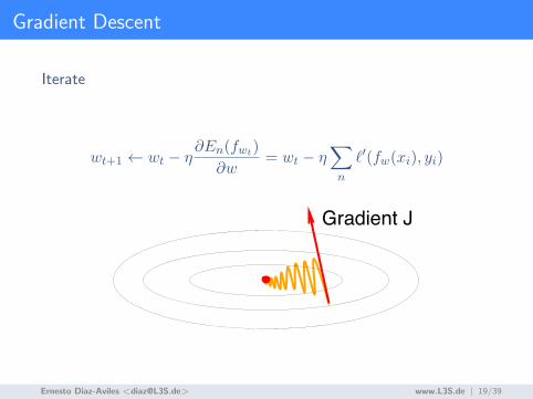
Gradient Descent
Iterate
wt+1 ← wt − η∂En(fwt)
∂w= wt − η
∑
n
`′(fw(xi), yi)
Gradient Descent (GD)
Iterate
• wt+1! wt " !"En(fwt)
"w
Gradient J
Best speed achieved with fixed learning rate ! = 1"max
.(e.g., Dennis & Schnabel, 1983)
Cost per Iterations Time to reach Time to reachiteration to reach # accuracy # E(fn)! E(f"F ) < $
GD O(nd) O!% log 1
#
"O
!nd% log 1
#
"O
!d2 %$1/& log2 1
$
"
– In the last column, n and # are chosen to reach # as fast as possible.– Solve for # to find the best error rate achievable in a given time.– Remark: abuses of the O() notation
Ernesto Diaz-Aviles <[email protected]> www.L3S.de | 19/39

Stochastic Gradient Descent
Iterate
Draw Random Example (xt, yy)
wt+1 ← wt − ηt `′(fwt(xt), yt)
Stochastic Gradient Descent (SGD)
Iterate
• Draw random example (xt, yt).
• wt+1! wt "!
t
"#(fwt(xt), yt)
"w
Total Gradient <J(x,y,w)>
Partial Gradient J(x,y,w)
Best decreasing gain schedule with ! = 1"min
.(see Murata, 1998; Bottou & LeCun, 2004)
Cost per Iterations Time to reach Time to reachiteration to reach # accuracy # E(fn)! E(f"F ) < $
SGD O(d) % k# + o
!1#
"O
!d % k
#
"O
!d % k
$
"
With 1 # k # &2
– Optimization speed is catastrophic.– Learning speed does not depend on the statistical estimation rate $.– Learning speed depends on condition number % but scales very well.
More info. at L. Bottou webpage: http://leon.bottou.org/
Ernesto Diaz-Aviles <[email protected]> www.L3S.de | 20/39

General Stochastic Gradient Descent Procedure for MF
SGD for MF
Input:Training data S; Regularization parameters λW and λH ;Learning rate η0; Learning rate schedule α; Number ofiterations T
Output: θ = (W,H)1: initialize W0 and H0
2: for t = 1 to T do3: (u, i, xui)← randomExample(S)4: wu ← wu − η ∂
∂wu`(xui, 〈wu,hi〉)− η λW wu
5: hi ← hi − η ∂∂hi
`(xui, 〈wu,hi〉)− η λH hi6: η = α · η7: end for8: return θT = (WT ,HT )
Ernesto Diaz-Aviles <[email protected]> www.L3S.de | 21/39

Pairwise Learning
(Bob, #EHEC)(Alice, #EHEC #Hannover) (Bob, #HUS)(Charlie, #HUS) (Charlie, #RKI) (Alice, #EHEC)... Monitor
#EHEC #Hannover #HUS #RKI
Alice 2 1 ? ?
Bob 1 ? 1 ?
Charlie ? ? 1 1
E.g, Pairwise Preferences for Alice: #EHEC > {#Hannover, #HUS, # RKI}#Hannover > {#HUS, #RKI}
Ernesto Diaz-Aviles <[email protected]> www.L3S.de | 22/39

CF Based on Matrix Factorization
Ranking Loss (pairwise):
L(P,W,H) =1
|P |∑
p∈Ph(yuij · 〈wu,hi − hj〉) , (1)
argminθ=(W,H)
L(P,W,H) +λW2||W||22 +
λH2||H||22 . (2)
where
h(z) = max(0, 1− z) is the hinge-loss;
yuij = sign(xui − xuj) is the sign(z) function, which returns+1 if z > 0, i.e., xui > xuj , and −1 if z < 0.
The prediction function 〈wu,hi − hj〉 = 〈wu,hi〉 − 〈wu,hj〉corresponds to the difference of predictor values xui − xuj .Gradient
−∇h(pt, θt) =
yuij · (hi − hj) if θr = wu,
yuij ·wu if θt = hi,
yuij · (−wu) if θt = hj ,
0 otherwise.
Ernesto Diaz-Aviles <[email protected]> www.L3S.de | 23/39

CF Based on Matrix Factorization
Ranking Loss (pairwise):
L(P,W,H) =1
|P |∑
p∈Ph(yuij · 〈wu,hi − hj〉) , (1)
argminθ=(W,H)
L(P,W,H) +λW2||W||22 +
λH2||H||22 . (2)
where
h(z) = max(0, 1− z) is the hinge-loss;
yuij = sign(xui − xuj) is the sign(z) function, which returns+1 if z > 0, i.e., xui > xuj , and −1 if z < 0.
The prediction function 〈wu,hi − hj〉 = 〈wu,hi〉 − 〈wu,hj〉corresponds to the difference of predictor values xui − xuj .
Gradient
−∇h(pt, θt) =
yuij · (hi − hj) if θr = wu,
yuij ·wu if θt = hi,
yuij · (−wu) if θt = hj ,
0 otherwise.
Ernesto Diaz-Aviles <[email protected]> www.L3S.de | 23/39

CF Based on Matrix Factorization
Ranking Loss (pairwise):
L(P,W,H) =1
|P |∑
p∈Ph(yuij · 〈wu,hi − hj〉) , (1)
argminθ=(W,H)
L(P,W,H) +λW2||W||22 +
λH2||H||22 . (2)
where
h(z) = max(0, 1− z) is the hinge-loss;
yuij = sign(xui − xuj) is the sign(z) function, which returns+1 if z > 0, i.e., xui > xuj , and −1 if z < 0.
The prediction function 〈wu,hi − hj〉 = 〈wu,hi〉 − 〈wu,hj〉corresponds to the difference of predictor values xui − xuj .Gradient
−∇h(pt, θt) =
yuij · (hi − hj) if θr = wu,
yuij ·wu if θt = hi,
yuij · (−wu) if θt = hj ,
0 otherwise.
Ernesto Diaz-Aviles <[email protected]> www.L3S.de | 23/39

Example of Model Update based on SGD for MF
Input: Stream representative sample at time t: St; Regularizationparameters λW , λH+ , and λH− ; Learning rate η0; Learning rateschedule α; Number of iterations Tθ
Output: θ = (W,H)1: procedure updateModel(St, λW , λH+ , λH− , η0, α, Tθ)2: for t = 1 to Tθ do3: ((u, i), (u, j))← randomPair(St) ∈ P4: yuij ← sign(xui − xuj)5: wu ← wu + η yuij (hi − hj)− η λW wu
6: hi ← hi + η yuij wu − η λH+ hi7: hj ← hj + η yuij (−wu)− η λH− hj8: η = α · η9: end for
10: return θ = (WTθ ,HTθ )11: end procedure
Ernesto Diaz-Aviles <[email protected]> www.L3S.de | 24/39

ScenarioTowards Real-time Collaborative Filtering for Big Fast Data
Ernesto Diaz-Aviles <[email protected]> www.L3S.de | 25/39

Scenario: #-tags Recommendation in Twitter
Top-N Recommendations
Recommendation of Interesting Topics ⇒ #-tags
Online Collaborative Filtering
Ernesto Diaz-Aviles <[email protected]> www.L3S.de | 26/39

Scenario: #-tags Recommendation in Twitter
Top-N Recommendations
Recommendation of Interesting Topics ⇒ #-tags
Online Collaborative Filtering
Ernesto Diaz-Aviles <[email protected]> www.L3S.de | 26/39

Scenario: #-tags Recommendation in Twitter
Top-N Recommendations
Recommendation of Interesting Topics ⇒ #-tags
Online Collaborative Filtering
Ernesto Diaz-Aviles <[email protected]> www.L3S.de | 26/39

Pairwise Learning
(Bob, #EHEC)(Alice, #EHEC #Hannover) (Bob, #HUS)(Charlie, #HUS) (Charlie, #RKI) (Alice, #EHEC)... Monitor
#EHEC #Hannover #HUS #RKI
Alice 2 1 ? ?
Bob 1 ? 1 ?
Charlie ? ? 1 1
E.g, Pairwise Preferences for Alice: #EHEC > {#Hannover, #HUS, # RKI}#Hannover > {#HUS, #RKI}
Ernesto Diaz-Aviles <[email protected]> www.L3S.de | 27/39

RMFO: Main Steps
Social Media Stream, e.g., Twitter
Sample the Stream
Real-time Personalized Recommendations
Online Matrix Factorization: Pairwise Approach for Personalized Rank Learning
Ernesto Diaz-Aviles <[email protected]> www.L3S.de | 28/39

RMFO: Sampling Strategies
Social Media Stream, e.g., Twitter
Sample the Stream
Real-time Personalized Recommendations
Online Matrix Factorization: Pairwise Approach for Personalized Rank Learning
Sampling Strategies
RMFO-SP: Single Pass
RMFO-UB: User Buffer
RMFO-RSV: ReservoirSampling
Ernesto Diaz-Aviles <[email protected]> www.L3S.de | 29/39

RMFO-SP: Single Pass
TwitterMonitor
Online Collaborative Filtering Pairwise MF
Real-time Personalized Recommendations
Model Update Using Single Pair at the Time
Ernesto Diaz-Aviles <[email protected]> www.L3S.de | 30/39
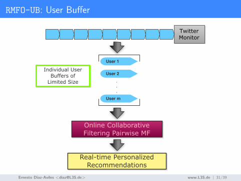
RMFO-UB: User Buffer
TwitterMonitor
Online Collaborative Filtering Pairwise MF
Real-time Personalized Recommendations
User 1
User 2
User m
.
.
.
Individual User Buffers of
Limited Size
Ernesto Diaz-Aviles <[email protected]> www.L3S.de | 31/39

RMFO-RSV: Reservoir Sampling
TwitterMonitor
Reservoir Sampling
Online Collaborative Filtering Pairwise MF
Real-time Personalized Recommendations
Ernesto Diaz-Aviles <[email protected]> www.L3S.de | 32/39

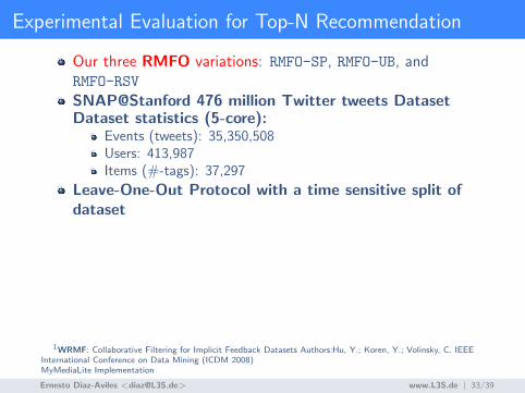
Experimental Evaluation for Top-N Recommendation
Our three RMFO variations: RMFO-SP, RMFO-UB, andRMFO-RSV
SNAP@Stanford 476 million Twitter tweets DatasetDataset statistics (5-core):
Events (tweets): 35,350,508Users: 413,987Items (#-tags): 37,297
Leave-One-Out Protocol with a time sensitive split ofdatasetMetric recall also known as hit-rate :
recall :=
∑u∈Utest 1[iu∈Top-Nu]
|Utest|
Baselines: (1) Trending Topics (TT) and (2) WeightedRegularized Matrix Factorization (WRMF)1
1WRMF: Collaborative Filtering for Implicit Feedback Datasets Authors:Hu, Y.; Koren, Y.; Volinsky, C. IEEEInternational Conference on Data Mining (ICDM 2008)MyMediaLite Implementation
Ernesto Diaz-Aviles <[email protected]> www.L3S.de | 33/39
Experimental Evaluation for Top-N Recommendation
Our three RMFO variations: RMFO-SP, RMFO-UB, andRMFO-RSV
SNAP@Stanford 476 million Twitter tweets DatasetDataset statistics (5-core):
Events (tweets): 35,350,508Users: 413,987Items (#-tags): 37,297
Leave-One-Out Protocol with a time sensitive split ofdataset
Metric recall also known as hit-rate :
recall :=
∑u∈Utest 1[iu∈Top-Nu]
|Utest|
Baselines: (1) Trending Topics (TT) and (2) WeightedRegularized Matrix Factorization (WRMF)1
1WRMF: Collaborative Filtering for Implicit Feedback Datasets Authors:Hu, Y.; Koren, Y.; Volinsky, C. IEEEInternational Conference on Data Mining (ICDM 2008)MyMediaLite Implementation
Ernesto Diaz-Aviles <[email protected]> www.L3S.de | 33/39

Experimental Evaluation for Top-N Recommendation
Our three RMFO variations: RMFO-SP, RMFO-UB, andRMFO-RSV
SNAP@Stanford 476 million Twitter tweets DatasetDataset statistics (5-core):
Events (tweets): 35,350,508Users: 413,987Items (#-tags): 37,297
Leave-One-Out Protocol with a time sensitive split ofdatasetMetric recall also known as hit-rate :
recall :=
∑u∈Utest 1[iu∈Top-Nu]
|Utest|
Baselines: (1) Trending Topics (TT) and (2) WeightedRegularized Matrix Factorization (WRMF)1
1WRMF: Collaborative Filtering for Implicit Feedback Datasets Authors:Hu, Y.; Koren, Y.; Volinsky, C. IEEEInternational Conference on Data Mining (ICDM 2008)MyMediaLite Implementation
Ernesto Diaz-Aviles <[email protected]> www.L3S.de | 33/39

Recommendation PerformanceTT (previous month)WRMFRankMF-SPRankMF-UBRankMF-RSV
Recall@1 Recall@5 Recall@10 Recall@15 Recall@20 Recall@30 Recall@40 [email protected] 0.0522 0.0780 0.0929 0.0943 0.1061 0.1132 0.12100.0885 0.1896 0.2573 0.3045 0.3406 0.3943 0.4331 0.46370.0357 0.1003 0.1469 0.1807 0.2078 0.2510 0.2859 0.31650.0377 0.1070 0.1555 0.1897 0.2169 0.2605 0.2955 0.32580.1040 0.2458 0.3215 0.3694 0.4048 0.4562 0.4942 0.5247
0
0.1
0.2
0.3
0.4
0.5
0.6
Top-1 Top-5 Top-10 Top-15 Top-20 Top-30 Top-40 Top-50
recall @ N
reca
ll
TT (previous month) WRMF RMFO-SP RMFO-UB RMFO-RSV
Ernesto Diaz-Aviles <[email protected]> www.L3S.de | 34/39

Recommendation Performance for Different Reservoir Sizes
recall@10 Reservoir Size
RMFO-RSV RankMF-UB-512
Trending Topics
(previous month)
WRMF (Batch)
0.5 0.0621339040754 0.1555 0.0780177217 0.25731384921 0.1143406622964 0.1555 0.0780177217 0.25731384922 0.1845008184564 0.1555 0.0780177217 0.25731384924 0.2611452241341 0.1555 0.0780177217 0.25731384928 0.3215161808443 0.1555 0.0780177217 0.2573138492
Recall@10Test Set Size (= n test users; leave one out)
260246
128 factors
0
0.05
0.10
0.15
0.20
0.25
0.30
0.35
0.40
0.5 2 3.5 5 6.5 8
Top-10: recall vs Reservoir Sizere
call
Reservoir Size (Millions)
RMFO-RSVRMFO-UB-512WRMF (Batch)Trending Topics (previous month)
Ernesto Diaz-Aviles <[email protected]> www.L3S.de | 35/39

Recommendation Performance and Dimensionality
RMFO-RSV 8M
8163264128WRMF-128
RMFO-RSV-8RMFO-RSV-16RMFO-RSV-32RMFO-RSV-64RMFO-RSV-128
Recall@1 Recall@5 Recall@10 Recall@15 Recall@20 Recall@30 Recall@40 Recall@50
0.0468 0.1529 0.2289 0.2811 0.3207 0.3787 0.4216 0.45570.0624 0.1830 0.2627 0.3146 0.3529 0.4080 0.4483 0.48030.0793 0.2118 0.2912 0.3407 0.3771 0.4297 0.4683 0.49880.0913 0.2284 0.3076 0.3570 0.3924 0.4431 0.4804 0.51010.1040 0.2458 0.3215 0.3694 0.4048 0.4562 0.4942 0.52470.0885 0.1896 0.2573 0.3045 0.3406 0.3943 0.4331 0.4637
8 0.2289 0.2573 0.0780177216 0.2627 0.2573 0.0780177232 0.2912 0.2573 0.0780177264 0.3076 0.2573 0.07801772
128 0.3215 0.2573 0.07801772
0
0.05
0.10
0.15
0.20
0.25
0.30
0.35
0.40
8 20 32 44 56 68 80 92 104 116 128
Top-10: Recall vs Number of Factorsre
call
Number of Factors
RMFO-RSVWRMF-128TT
Ernesto Diaz-Aviles <[email protected]> www.L3S.de | 36/39

Time and Space Savings vs Recommendation Quality
Method Time recall@10 Space Gain Gain in(128 factors) (seconds) in speed recall
WRMF (Baseline) 23127.34 0.2573 100.00% – –
RMFO-RSV 0.5 M 47.97 0.0621 1.41% 482.16 -75.85%
RMFO-RSV 1 M 89.15 0.1143 2.83% 259.42 -55.56%
RMFO-RSV 2 M 171.18 0.1845 5.66% 135.11 -28.30%
RMFO-RSV 4 M 329.60 0.2611 11.32% 70.17 +1.49%
RMFO-RSV 8 M 633.85 0.3215 22.63% 36.49 +24.95%
RMFO-RSV INF 1654.52 0.3521 100.00% 13.98 +36.84%
Ernesto Diaz-Aviles <[email protected]> www.L3S.de | 37/39

Conclusions
Matrix Factorization: Powerful Machine Learning approach forTop-N Recommendation
SGD for MF : Large Scale Datasets
RMFO approach for recommending topics to users in presenceof streaming data
RMFO achieves state-of-the-art performance in terms ofrecommendation quality with significant improvements inspeed and space efficiency
Ernesto Diaz-Aviles <[email protected]> www.L3S.de | 38/39

Thank you!
Your Software Project and Thesis at L3S Research Center :)
Ernesto Diaz-Aviles
Ernesto Diaz-Aviles <[email protected]> www.L3S.de | 39/39

www.L3S.de

More Info
www.L3S.de