Embed Size (px)
Citation preview
Draft
MATRIX COMPLETION VIA NON-CONVEXPROGRAMMING
By Diego Franco Saldana and Haolei Weng
We consider the matrix completion problem in the noisy setting.To achieve statistically efficient estimation of the unknown low-rankmatrix, solving convex optimization problems with nuclear norm con-straints has been both theoretically and empirically proved a success-ful strategy under certain regularity conditions. However, the bias in-duced by the nuclear norm penalty may compromise the estimationaccuracy. To address this problem, following a parallel line of researchin sparse regression models, we study the performance of a family ofnon-convex regularizers in the matrix completion problem. In partic-ular, a fast first-order algorithm is proposed to solve the non-convexprogramming problem. We also describe a degree-of-freedom basedreparametrization to “refine” the search along the solution path. Nu-merical experiments show that these non-convex methods outperformthe traditional use of nuclear norm regularization in both simulatedand real data sets.
1. Introduction. The matrix completion problem consists in the re-covery of a data matrix based on a sampling of its entries [1]. A popularexample is the Netflix competition [2]. Denote the data matrix by Mm×n,the rows corresponding to users and columns to movies. The entry Mij is therating user i gives to movie j. Typically, users only rate a few movies so thatthere is only a small fraction of the matrix M observed. Netflix would liketo complete this matrix in order to recommend potentially appealing moviesto users. Generally, it is impossible to correctly predict the ratings of usersfor unseen movies without additional information about M . A useful fact isthat M is approximately low-rank because ratings are mainly determinedby a small number of factors such as movie genre and user taste.
This problem can be formulated in a more familiar way to the statis-tics literature. Let β ∈ Rmn be the long vector obtained after stacking thecolumns of data matrix Mm×n. The observed entries form a shorter vectorY = Xβ, where the matrix Xk×mn (k is the number of observations) is alinear operator mapping the data matrix to its observed entries. Since it isfairly common to have k mn in many statistical applications, the ma-trix completion problem can be considered as a high-dimensional regressionproblem. Based on the response Y and design matrix Xk×mn, the objective
Keywords and phrases: Low-Rank, Nuclear Norm, Soft-Thresholding, Singular ValueDecomposition, Non-Convex Penalty, Degrees-of-freedom, Recalibration.
1
Draft
2
is to estimate the coefficient vector β. It is well known that high-dimensionalregression problems require extra structure in β to make statistical inferencefeasible. An active line of research consists in estimating a sparse β with onlya few non-zero components [3, 4, 5, 6]. In our case, the structure of interestin the data matrix Mm×n is low-rank instead of sparsity. Although the ma-trix completion problem can be framed into the high-dimensional regressionframework, it distinguishes itself as a more difficult problem in two respects.Firstly, from a computational point of view, the dimensionality of β caneasily scale to the tens of millions and above. More importantly, low-rankinducing optimization problems involve advanced algorithmic analysis suchas characterizing the subgradient of nuclear norm. Secondly, as well knownin sparse regression setting, to achieve optimal estimation of β, the designmatrix needs to be well “conditioned”. For instance, the Restricted IsometryProperty (RIP) in [6] requires that every set of columns with cardinality lessthan a given number behaves like an orthonormal system. However, due tothe sampling nature of the matrix completion problem, Xk×mn never satis-fies RIP [7]. Therefore, a less restrictive condition on X, or a more delicatelow rank structure on β is required to recover the data matrix Mm×n.
The report is organized as follows. We give a brief literature survey onthe theoretical developments in estimating low-rank matrices in Section 2.In Section 3, we review a few algorithms for solving convex optimizationproblems with nuclear norm constraints. We then propose and study a non-convex programming approach in Section 4. Numerical experiments are con-ducted in Section 5. Section 6 discusses potential research directions andopen problems.
2. Matrix Completion Theory. To fix notations, denote the un-known low-rank matrix by Mm×n (m ≥ n) with rank r, and the set of loca-tions corresponding to observed entries of M by Ω. Let k be the cardinality ofΩ. PΩ is the projection mapping such that (PΩ(X))ij = Xij if (i, j) ∈ Ω and(PΩ(X))ij = 0 if (i, j) /∈ Ω. For a vector a, ‖a‖pp =
∑i |ai|p (1 ≤ p ≤ +∞).
For any matrix A, ‖A‖∗ =∑σi(A), ‖A‖2F =
∑σ2i (A), ‖A‖2 = σ1(A), where
σ1(A) ≥ σ2(A) ≥ · · · ≥ σr(A) ≥ 0 are singular values of A.
2.1. Exact Matrix Completion. The first theoretical guarantee for exactrecovery of a low-rank matrix appeared in the compressed sensing commu-nity [1]. The problem is to exactly recover M based on PΩ(M). The authorsin [1] propose the following convex optimization approach,
minimize ‖X‖∗(2.1)
subject to PΩ(X) = PΩ(M).
Draft
MATRIX COMPLETION VIA NON-CONVEX PROGRAMMING 3
A surprising result shown in their paper is that this simple approach canachieve exact recovery for a broad family of “incoherent” matrices. LetM = UΣV T be the SVD of M with U = (u1, . . . , ur) and V = (v1, . . . , vr).Incoherence as defined in [1] is characterized by two conditions:
A. max1≤i≤mmr ‖U
T ei‖22 ≤ µ0, max1≤j≤nnr ‖V
T ej‖22 ≤ µ0
B. max1≤i≤m,1≤j≤n√
mnr (UV T )ij ≤ µ1,
where (ei) is the standard basis, and µ0, µ1 are two constants. Condition Arequires the row and column spaces of M to be diffuse such that informationabout unseen entries can be inferred from the observed ones. The main resultin [1] claims that
If M satisfies conditions A and B, and the observed set Ω is sampled uniformlyat random, with r ≤ µ−1
0 m1/5, k ≥ Cµ0m6/5r(β logm), then the solution to
(2.1) is unique and equal to M with probability at least 1− cm−β .
Essentially, a low-rank matrix M with incoherence constant µ0 = O(1) canbe exactly recovered through Θ(m6/5r logm) entries with high probability.A fundamental and interesting observation is that any m × n matrix ofrank r depends on (m + n − r)r degrees of freedom. Clearly, exact matrixrecovery is impossible if the number of observations is less than this intrinsicdimensionality. But, is it possible to recover M with a minimum numberof measurements approaching the above limit (at least up to logarithmicmultiplicative factors)? This problem has been addressed in [8]. The authorsintroduce the “strong incoherence” condition:
C. | < Uei, Uej > − rmI(i=j)| ≤ µ2
√rm , 1 ≤ i, j ≤ m,
| < V ei, V ej > − rnI(i=j)| ≤ µ2
√rn , 1 ≤ i, j ≤ n.
M is said to obey the “strong incoherence” property with parameter µ if itsatisfies conditions B and C with max(µ1, µ2) ≤ µ. Condition C is generallymore restrictive than condition A. For instance, condition C implies thatmr ‖U
T ei‖ ≤ 1 + µ2√r
and nr ‖V
T ej‖ ≤ 1 + µ2√r. The authors in [8] show that
If M obeys the strong incoherence property with parameter µ, and the ob-served set Ω is sampled uniformly at random with k ≥ Cµ2mr log6 m, thenM is the unique solution to (2.1) with probability at least 1−m−3.
For strong incoherent matrices with µ = O(1), the number of measure-ments sufficient for exact recovery can be reduced from Θ(m6/5r logm)to Θ(mr log6m). The authors further prove that, under a Bernoulli modelwhere each entry is independently observed with probability k
n2 (m = n),
if − log(1 − km2 ) ≥ µ0r
m log(m2δ ) does not hold, it is impossible to recover anincoherent matrix M with parameter µ0 by any algorithm with probabilitylarger than δ. In other words, a necessary condition to guarantee success
Draft
4
with probability at least δ is that
k ≥ m2(1− e−µ0rm
log m2δ ).
When µ0rm log m
2δ = o(1), it follows that k = Θ(µ0mr log(m2δ )). That is tosay, to recover an incoherent matrix with constant µ0, the simple convexapproach (2.1) only requires minimum (up to logarithmic factors) observa-tions.
The proofs provided in [1, 8] involve sophisticated algebra manipulationsand moment inequality arguments which are highly technical. More recently,[9] presented a much easier proof and sharpened the previous results. Thispaper shows that
If M satisfies conditions A and B, and the observed set Ω is sampled uniformlyat random, with k ≥ 32 maxµ2
1, µ0r(n+m)β log2(2m) for β > 1, then M isthe unique solution to (2.1) with probability at least 1−6 log(m)(n+m)2−2β−m2−2β1/2
.
For µ0 = O(1), the number of measurements needed is Θ(µ21rm log2m).
For a large proportion of incoherent matrices, [1] shows that µ1 = O(logm).Thus, k only needs to be of the order Θ(rm log4m). The proof in [9] isrelatively simple; it is adapted from the quantum information communityand only uses basic matrix analysis and concentration inequalities.
Note that the uniform sampling assumption appears in all results providedin [1, 8, 9]. Rather than being an intrinsic statistical modeling concern, theseauthors introduce the uniform sampling assumption in order to avoid worst-case sampling behavior. In reality, however, uniform sampling is likely tobe an improper assumption. For example, in the Netflix data set, popularmovies have more ratings and active users rate more movies than averageusers. The ratings available are expected to be highly non-uniform. Moreimportantly, the key incoherence condition required in [1, 8, 9] is mainlyfor uniform sampling to capture the essential information in M with highprobability. If the sampling can be adapted to the structure of M (e.g.,more important entries are more likely to be sampled), then the incoherenceconditions can be weakened. This is the spirit of [10], which defines the localcoherences as follows:
µi =m
r‖UT ei‖2, i = 1, . . . ,m.
νj =n
r‖V T ej‖2, j = 1, . . . , n.
The authors prove that
If M has local coherence parameters µi, νj, and each element (i, j) is inde-
pendently observed with probability pij such that pij ≥ minc0
(µi+νj)r log2(n+m)
n, 1
,
Draft
MATRIX COMPLETION VIA NON-CONVEX PROGRAMMING 5
pij ≥ 1n10 , then M is the unique solution to (2.1) with probability at least
1− c1(n+m)−c2 , for some universal constants c0, c1, c2 > 0.
Note that the expected number of observed entries satisfies
∑i,j
pij ≥ maxc0r log2(n+m)
n
∑i,j
(µi + νj),∑i,j
1
n10
= 2c0mr log2(n+m)
which does not depend on the local coherence parameters. The Azuma-Hoeffding inequality then implies
Under the local coherence sampling given by the pij above, the matrix M isunique solution to (2.1) and k ≤ 3c0mr log2(m+ n) with probability at least
1− c′1(n+m)−c′2 .
For M with incoherence parameter µ0, it is easy to see that µi ≤ µ0 andνj ≤ µ0. Hence, considering uniform sampling as a very special case of
local coherence sampling with probability pij ≥ cµ0r log2mn , criterion (2.1)
exactly recovers M using k = Θ(µ0mr log2m) entries with high probability.For µ0 = O(1), k = Θ(mr log2m) achieves the best existing scaling. Moreinterestingly, condition B is dropped!
2.2. Stable Matrix Completion. In the real world, observations are likelycorrupted by noise. Thus, a more realistic model is
Yij = Mij + Zij , (i, j) ∈ Ω,
where (Zij) are zero-mean noise terms and (Yij) are observations. Under thismodel, criterion (2.1) tends to overfit. To achieve a better bias and variancetrade-off, the authors in [7] propose to solve
minimize ‖X‖∗(2.2)
subject to ‖PΩ(X − Y )‖F ≤ δ,
under the assumption that ‖PΩ(Z)‖F ≤ δ. Let the minimizer of (2.2) be M .In [7], it is shown that
If M satisfies the strong incoherence condition, then with high probability, Mobeys
(2.3) ‖M −M‖F ≤ 4
√(2 + p)n
pδ + 2δ,
where p = kmn
.
Draft
6
The error upper bound is approximately of the order√
np δ. To have a bet-
ter understanding of the bound, [7] compares it with two additional errorbounds. The first one assumes the linear sampling operator A obeys theRIP,
(1−∆)‖X‖2F ≤1
p‖A(X)‖2F ≤ (1 + ∆)‖X‖2F
for all small rank matrices X and ∆ < 1. Note that the RIP does not holdfor the linear operator PΩ. Then, with high probability, M obeys
‖M −M‖F ≤ C0p−1/2δ
The second one considers an oracle estimator. Let the tangent space of Mbe
T (M) = UXT + Y V T | X ∈ Rn×r, Y ∈ Rm×r.
The linear space T (M) is the analogous to the vector space with the samesupport as the least squares estimator in the linear regression setting. Sup-pose we have prior information about T , then a natural approach is solving
minimize ‖PΩ(X)− PΩ(Y )‖F(2.4)
subject to X ∈ T (M).
It it shown in [7] that the minimizer M of (2.4) obeys
‖M −M‖F ≈ p−1/2δ.
In summary, the convex programming criterion (2.2) achieves stable matrixcompletion (error proportional to noise level), but loses efficiency by a fac-tor of
√n, compared to the oracle estimator and the “compressed sensing”
estimator assuming the RIP.A remarkably different approach using non-convex methods is proposed
in [11]. The basic idea is as follows:
1. Trim PΩ(Y ) by setting the rows and columns with many revealedentries to zero.
2. Calculate the best rank r approximation to the trimmed matrix.3. Minimize the cost function F (P,Q) = minS∈Rr×r F(P,Q, S), whereF(P,Q, S) = 1
2
∑(i,j)∈Ω(Yij − (PSQT )ij)
2.
Step 3 is solved by using a gradient descent algorithm on matrix manifolds,where the projected trimmed matrix serves as an initial point. In practice,however, the rank r has to be estimated. For the method to work, [11]introduces a slightly different incoherent condition:
Draft
MATRIX COMPLETION VIA NON-CONVEX PROGRAMMING 7
D. max1≤i≤m,1≤j≤n√
mnr |∑r
l=1 Uil(σl/σ1)Vjl| ≤ µ3,
where σ1 ≥ · · · ≥ σr > 0 are the nonzero singular values of the matrix M .Let κ = σ1
σrand the non-convex method estimator be M∗. The authors in
[11] show that
If M obeys conditions A and D, and Ω is sampled uniformly at random withk ≥ C
√mnκ2 maxµ0r
√mn
logn, µ20r
2mnκ4, µ2
3r2mnκ4, then with probability
at least 1− 1/n3,
(2.5)1√mn‖M∗ −M‖F ≤ C′κ2
√rmn
k‖PΩ(Z)‖2.
The bound given in [7] can be nearly reformulated as
(2.6)1√mn‖M −M‖F ≤ 7
√n
k‖PΩ(Z)‖F +
2√mn‖PΩ(Z)‖F .
Generally, M∗ and M are not directly comparable since M requires thestrong incoherence condition while M∗ needs the condition number κ tobe bounded. In terms of the error bound, expression (2.5) does not includethe second term in (2.6). Suppose m = n, then error bound in (2.5) isΘ(nk√r‖PΩ(Z)‖2) while the first term in (2.6) is Θ(
√nk ‖PΩ(Z)‖F ). In the
case where PΩ(Z) is i.i.d Gaussian with variance τ2 and rank r = o(n), itis shown in [11] that the bound in (2.5) is Θ(τ
√nrk ), having the same order
as the oracle estimator provided in [7].An alternative way to estimate the low-rank matrix is optimizing a pe-
nalized loss function as widely seen in the regression setting:
minX
1
2‖PΩ(Y )− PΩ(X)‖2F + λ‖X‖∗ .
The authors in [12] study this type of estimator in a more general settingwith approximately low-rank structures and weighted sampling. For simplic-ity, we only present their results for exact low-rank matrices under uniformsampling of the observations. The key idea in establishing an error boundfor the corresponding M-estimator is deriving a restricted strong convexity(RSC) condition as proposed in the unified framework introduced in [13]:
(2.7)‖PΩ(X)‖F√
n≥ c‖X‖F .
As is easily seen, inequality (2.7) does not hold (with high probability) formatrices with only one nonzero entry. To avoid these overly “spiky” matrices,the authors in [12] define a tractable measure of “spikiness” as
(2.8) αsp(X) =√mn‖X‖∞‖X‖F
,
Draft
8
where ‖X‖∞ is the elementwise `∞-norm. Note that 1 ≤ αsp ≤√mn, with
αsp = 1 when X has entries that are all equal, and αsp =√mn if X has a
single nonzero entry. The authors consider the M-estimator
M ∈ arg min‖X‖∞≤ α∗√
mn
1
2k‖PΩ(X)− PΩ(Y )‖2F + λn‖X‖∗ ,
where α∗ ≥ 1 is a measure of “spikiness”. Assuming n = m, it has beenshown in [12] that
If PΩ(Z) is i.i.d. sub-exponential with variance τ2, M has rank at most r,
Frobenius norm at most 1, and αsp(M) ≤ α∗, then M with λn = 4τ√
n lognk
obeys
(2.9) ‖M −M‖2F ≤ c′1 maxτ2, 1(α∗)2 rn logn
k+c1(α∗)2
k
with probability at least 1− c2e−c3 logn.
To examine how good the proposed M-estimator is, the authors furtherestablish an information-theoretic lower bound. Define the minimax risk inFrobenius norm
B(r) = X ∈ Rn×n | rank(X) ≤ r, αsp(X) ≤√
32 log nR(B(r)) = inf
Msup
M∈B(r)E[‖M −M‖2F ] .
Then, there is a universal constant c > 0 such that
R(B(r)) ≥ cτ2 rn
k.
The dominant term in (2.9) matches the minimax lower bound up to log-arithmic factors. The spikiness condition is essentially different from theincoherence or strong incoherence conditions introduced in [7, 11]. The in-coherence conditions only involve the left and right singular vectors of M ,while the spikiness condition also depends on its singular values. For exactrecovery in the noiseless setting, dependency only on the singular vectorsis reasonable because they determine the tangent space of M . In the noisycase, however, the authors argue that additional conditions on the singularvalues also play an important role. They point out an example where theirspikiness condition holds and incoherence conditions are violated. The de-tailed comparison of error bounds with those in [7, 11] can also be found in[12].
Draft
MATRIX COMPLETION VIA NON-CONVEX PROGRAMMING 9
2.3. General Low Rank Matrix Estimation. The sampling nature of PΩ
makes the theoretical development of the matrix completion problem ofparticular interest. On the other hand, there are several applications apartfrom the matrix completion setting that also explore low-rank structures ofdata matrices. Examples include compressed sensing, face recognition andmultivariate regression [14, 15]. Thus, a general set up is
Y = A(M) + Z ,
where A is a general linear operator and Z is the noise matrix. A naturalapproach in estimating M is solving
(2.10) minX
‖Y −A(X)‖2F + λn‖X‖G ,
where ‖X‖G is a low-rank inducing penalty such as nuclear norm or Schattenp-norm. We refer to the papers [14, 15, 16, 17] for a detailed theoretical studyof this general approach.
3. Matrix Completion Algorithms. We consider solving two opti-mization problems. Namely, the exact recovery approach
minimize ‖X‖∗(3.1)
subject to PΩ(X) = PΩ(M) ,
and the stable recovery method
minX
1
2‖PΩ(X)− PΩ(Y )‖2F + λ‖X‖∗ .(3.2)
In [17], it is shown that
‖X‖∗ = minW1,W2
1
2(tr(W1) + tr(W2))(3.3)
s.t.
[W1 XXT W2
] 0.
Hence, (3.1) can be reformulated as the semidefinite programming problem:
minX,W1,W2
1
2(tr(W1) + tr(W2))(3.4)
s.t.
[W1 XXT W2
] 0
PΩ(X) = PΩ(M) .
Draft
10
Interior-point methods are readily available to solve (3.4). However, thistype of algorithms are not scalable to large matrices with over a millionentries. The authors in [18] propose a fast, first-order algorithm which ex-plores low-rank and sparse matrix structures to save computational andstorage cost. The idea is to approximate the solution of (3.1) by solving asequence of closely related problems as follows
minimize τ‖X‖∗ +1
2‖X‖2F(3.5)
subject to PΩ(X) = PΩ(M) .
The unique solution Xτ of (3.5) can be efficiently calculated by a Lagrangemultiplier method. As τ → ∞, Xτ converges to the solution of (3.1). Weskip the implementation details here and focus instead on (3.2).
Problem (3.2) belongs to a generic class of optimization problems of theform
(3.6) minx
F (x) = f(x) + g(x)
,
where f(x) is a continuously differentiable convex function with Lipschitzcontinuous gradient L(f), and g(x) is a continuous convex function which ispossibly non-smooth. The authors in [19] present a fast iterative algorithmwhich solves an approximation problem at each iteration:
xt+1 = arg minx
QL(x, xt) = f(xt)+ < x−xt,∇f(xt) > +
L
2‖x−xt‖2+g(x)
.
Equivalently,
(3.7) xt+1 = arg minx
L
2‖x− (xt −
1
L∇f(xt))‖2 + g(x) .
It has been shown in [19] that
If xt is the sequence generated by (3.7), then for any t ≥ 1, F (xt)−F (x∗) ≤L(f)‖x0−x∗‖2
2t, where x∗ is any solution to (3.6).
The key issue in this algorithm is choosing L, which is analogous to selectinga step size in gradient search methods. Without knowing L(f), L can bechosen adaptively at each iteration with backtracking while still enjoying thesame convergence properties. The authors further introduce an acceleratedversion of (3.7) to improve the complexity from O(1/t) to O(1/t2). We referinterested readers to [19] for additional details. Back to (3.2), the convexfunction 1
2‖PΩ(X) − PΩ(Z)‖2F is continuously differentiable and λ‖X‖∗ is
Draft
MATRIX COMPLETION VIA NON-CONVEX PROGRAMMING 11
continuous and convex. In order to apply this algorithm, the key step issolving (3.7)
Xt+1 = arg minX
L
2‖X − (Xt +
1
L(PΩ(Y )− PΩ(Xt)))‖2F + λ‖X‖∗ .
Define the soft-thresholding operator Sλ,
Sλ(X) = USλ(Σ)V T , Sλ(Σ) = diag((σi − λ)+),
where X = UΣV T is the SVD of X and Σ = diag(σ1, . . . , σr). A crucialpoint is that Xt+1 can be obtained by soft-thresholding (see, for example,[18])
(3.8) Xt+1 = Sλ/L(Xt +1
L(PΩ(Y )− PΩ(Xt))) .
A similar iterative formula appears in [20], but derived from a differentperspective. The authors use a fixed point iterative method inspired by [22].The argument is as follows: X∗ is a solution to (3.2) if and only if
0 ∈ λ∂‖X∗‖+ PΩ(X∗)− PΩ(Y ) .
Equivalently,
0 ∈ τλ∂‖X∗‖+X∗ − [X∗ − τ(PΩ(X∗)− PΩ(Y ))] (τ > 0) .
Let Y ∗ = [X∗ − τ(PΩ(Y )− PΩ(X∗))], then X∗ is the optimal solution to
minX
1
2‖X − Y ∗‖2F + τλ‖X‖∗ .
Similar to (3.8), we then have
X∗ = Sτλ(X∗ − τ(PΩ(Y )− PΩ(X∗))) .
Thus, X∗ is a fixed point of the function Sτλ(X − τ(PΩ(Y )− PΩ(X))), anda natural iterative approach is
(3.9) Xt+1 = Sτλ(Xt − τ(PΩ(Y )− PΩ(Xt))) .
Iterations (3.8) and (3.9) take the same form when τ = 1L . Let A be the
matrix mapping the vectorized Vec(X) to its observed entries, then [20]proves that
The sequence Xt generated by (3.9) with τ ∈ (0, 2/λmax(ATA)) convergesto an optimal solution of (3.2).
Draft
12
The authors in [21] provide an alternative way to tackle (3.2). The idea isto iteratively impute the unobserved entries, and solve the imputed versionof (3.2) by soft-thresholding. It turns out this algorithm fits into the generalclass of minorize-maximize (MM) algorithms [23], an extension of the well-known EM algorithms. Let FY (X) = 1
2‖PΩ(X) − PΩ(Y )‖2F + λ‖X‖∗ andQY (X;Z) = 1
2‖X −PΩ⊥(Z)−PΩ(Y )‖2F + λ‖X‖∗. Then for any X, we have
QY (X;Z) =1
2‖PΩ(X)− PΩ(Y ) + PΩ⊥(X)− PΩ⊥(Z)‖2F + λ‖X‖∗
=1
2‖PΩ(X)− PΩ(Y )‖2F +
1
2‖PΩ⊥(X)− PΩ⊥(Z)‖2F + λ‖X‖∗
≥ FY (X)
and QY (Z;Z) = FY (Z). Thus, at each iteration, the updating rule is asfollows:
Xt+1 = arg minX
QY (X;Xt)(3.10)
= Sλ(PΩ(Y ) + PΩ⊥(Xt))
= Sλ(Xt + PΩ(Y )− PΩ(Xt)) .
Since Xt + PΩ(Y ) − PΩ(Xt) = PΩ(Y ) + PΩ⊥(Xt), at each step, we imputethe unobserved entries with the corresponding entries from the estimate inthe previous step. Iterations (3.8), (3.9) and (3.10) are all equal when τ = 1and L = 1. The nice thing about procedure (3.10) is that FY (Xt) is anon-increasing sequence since
FY (Xt+1) ≤ QY (Xt;Xt) = FY (Xt) .
It is further shown in [21] that
The sequence Xt generated by (3.10) converges to X∗, an optimal solution
of (3.2). Besides, FY (Xt) − FY (X∗) ≤ 2‖X0−X∗‖2Ft+1
, where X0 is an initialvalue.
To make the algorithm scalable to large matrices, the authors present anefficient way to speed up the SVD calculation in (3.10). Note that PΩ(Y )−PΩ(Xt) is a sparse matrix, and Xt is a low-rank matrix because of thesoft-thresholding operation. This “sparse+low rank” matrix structure canremarkably reduce the computational cost of matrix multiplication. TheSVD calculation is then performed by power methods, whose building blocksare matrix-vector multiplications.
The authors in [24] solve (3.2) by considering the equivalent problem
(3.11) min‖X‖∗≤µ2
1
2‖PΩ(X)− PΩ(Y )‖2F .
Draft
MATRIX COMPLETION VIA NON-CONVEX PROGRAMMING 13
Equivalence means that for any λ and any optimal solution X∗ of (3.2),there exists a µ ≥ 0 such that X∗ is also a solution to (3.11), and vice versa.By (3.3), it follows that (3.11) is also equivalent to solving
(3.12) minZ∈R(n+m)×(n+m)
Z0,tr(Z)=µ
1
2‖PΩ(X)− PΩ(Y )‖2F ,
where Z =
[A XXT B
]. Under this formulation, [24] follows a simple gradient
descent type algorithm proposed in [25]. The algorithm guarantees ε-smallprimal-dual error after at most O(1
ε ) iterations. At each iteration, the maincost is in calculating an approximate largest eigenvector of a given matrix.
4. Matrix Completion via Non-convex Programming.
4.1. A Family of Non-convex Penalties. We consider the matrix comple-tion problem in the noisy setting
(4.1) PΩ(Y ) = PΩ(M) + PΩ(Z) .
In section 1 we discussed that (4.1) can be treated as a high-dimensional lin-ear regression model; completing the matrix is equivalent to estimating thecoefficient parameter β ∈ Rmn. As the `1-penalty induces bias in estimationin the sparse setting, the nuclear norm also biases the estimation of singularvalues, and thus of low-rank matrices. Motivated by [26], we propose solvingthe non-convex optimization problem
(4.2) minX
Gλ,γ(X;Y ) =1
2‖PΩ(X)− PΩ(Y )‖2F + λ
∑i
P (σi;λ, γ) ,
where λP (σi;λ, γ) is the MC+ family of penalties [5] defined by
(4.3) λP (t;λ, γ) = λ(|t| − t2
2λγ)I(|t| < λγ) +
λ2γ
2I(|t| ≥ λγ) .
The reason why we choose this family of non-convex penalties is based onthe following one-dimensional problem
(4.4) Sγ(β, λ) = arg minβ
1
2(β − β)2 + λP (|β|;λ, γ) .
In this simplest scenario, the MC+ penalized estimator has an explicit formwhen γ > 1:
(4.5) Sγ(β, λ) =
0 if |β| ≤ λsign(β)( |β|−λ1−1/γ ) if λ < |β| ≤ λγβ if |β| > λγ .

Draft
14
We list a few desirable properties of the univariate minimizer Sγ(β, λ) whichare well explained in [26]:
1. Criterion (4.4) is strictly convex and Sγ(β, λ) is unique.2. Sγ(β, λ) is a continuous function of β.3. Sγ(β, λ) is a continuous function of γ on (1,∞).4. Sγ(β, λ) bridges the gap between soft-thresholding (`1) and hard-thresholding
(`0). In particular, as γ → +∞, Sγ(β, λ) → sign(β)(|β| − λ)+; and asγ → 1+, Sγ(β, λ)→ βI(|β| ≥ λ).
4.2. Fast First Order Algorithm. We follow the general procedure in [21]to solve (4.2). At each iteration, we compute
(4.6) Xt+1 = arg minX
1
2‖X − PΩ(Y )− PΩ⊥(Xt)‖2F + λ
∑i
P (σi;λ, γ) ,
where the σi are the singular values of X. The following proposition pro-vides a closed form expression for Xt+1.
Proposition 4.1. In (4.6), for any γ > 1, Xt+1 is unique. Define thespectral mapping Sλ,γ : Rm×n → Rm×n by Sλ,γ(X) = USλ,γ(Σ)V T , withSλ,γ(Σ) = diag(Sγ(σi, λ)), where X = UΣV T is the SVD of X. ThenXt+1 has the closed form expression
(4.7) Xt+1 = Sλ,γ(PΩ(Y ) + PΩ⊥(Xt)).
Proof. The proof is a direct application of von Neumann’s trace inequal-ity (A.1) given in Appendix A. Let W = PΩ(Y ) + PΩ⊥(Xt), the inequalityimplies
1
2‖X −W‖2F + λ
∑i
P (σi;λ, γ) =1
2
tr(XTX) + tr(W TW )− 2tr(XTW )
+λ∑i
P (σi;λ, γ)
(a)
≥ 1
2
∑i
σ2i +
∑i
σi(W )2 − 2∑i
σiσi(W )
+λ∑i
P (σi;λ, γ)
=∑i
1
2(σi − σi(W ))2 + λP (σi;λ, γ)
.
Draft
MATRIX COMPLETION VIA NON-CONVEX PROGRAMMING 15
The sum on the right-hand side is separable. By (4.5), there exists a uniqueσi = Sγ(σi(W ), λ) minimizing each term. To achieve the equality in (a), Xand W should share the same singular vectors.
Proposition 4.2. The sequence Gλ,γ(Xt);Y is non-increasing, whereXt is generated by iteration (4.7). Further, any local optimum of (4.2) isa fixed point of Sλ,γ(PΩ(Y ) + PΩ⊥(X)), as a function of X.
Proof.
Gλ,γ(Xt+1;Y ) = arg minX
1
2‖X − PΩ(Y )− PΩ⊥(Xt)‖2F + λ
∑i
P (σi;λ, γ)
≤ 1
2‖Xt − PΩ(Y )− PΩ⊥(Xt)‖2F + λ
∑i
P (σi(Xt);λ, γ)
=1
2‖PΩ(Xt)− PΩ(Y )‖2F + λ
∑i
P (σi(Xt);λ, γ)
= Gλ,γ(Xt;Y ) .
Let H(X) = 12‖X − PΩ(Y ) − PΩ⊥(X∗)‖2F + λ
∑i P (σi;λ, γ), where X∗ is a
local optimum of Gλ,γ(X;Y ). Then X∗ is a fixed point if and only if
X∗ = arg minX
H(X) .
This is true since, for anyX ∈ X : ‖X−X∗‖F ≤ r such thatGλ,γ(X∗;Y ) ≤Gλ,γ(X;Y ), we have
H(X) ≥ 1
2‖PΩ(X)− PΩ(Y )‖2F + λ
∑i
P (σi(X);λ, γ)
= Gλ,γ(X;Y ) ≥ Gλ,γ(X∗;Y )
=1
2‖X∗ − PΩ(Y )− PΩ⊥(X∗)‖2F + λ
∑i
P (σi(X∗);λ, γ)
= H(X∗) .
Thus, X∗ is also a local optimum of H(X). If the mapping H(·) is convex,then sinceH has only one global optimum, the local optimumX∗ must be theunique solution. It remains to show H(X) is a convex function of X. Withoutloss of generality, we prove H(X) = 1
2‖X −W‖2F + λ
∑i P (σi(X);λ, γ) is
convex. Note that
H(X) = −tr(W TX)+∑i
σi(W )σi+∑i
1
2(σi−σi(W ))2+λP (σi(X);λ, γ)
,
Draft
16
λ
γ
(λn−1, γn−1)
(λn, γn−1)
(λn−1, γn)
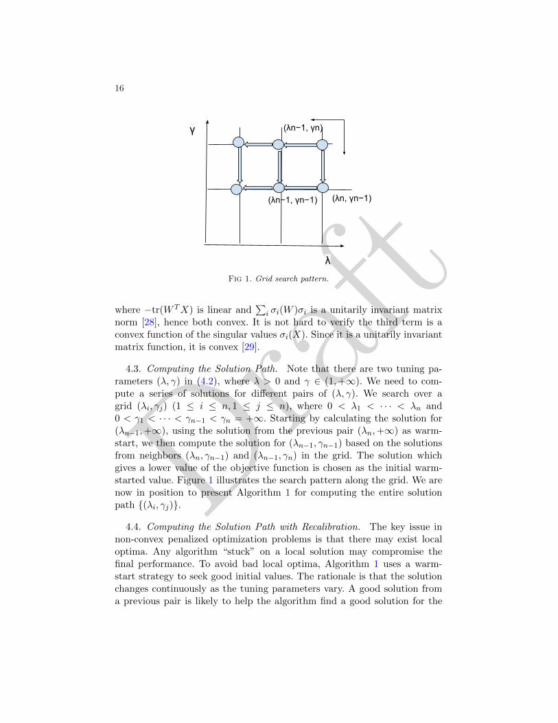
Fig 1. Grid search pattern.
where −tr(W TX) is linear and∑
i σi(W )σi is a unitarily invariant matrixnorm [28], hence both convex. It is not hard to verify the third term is aconvex function of the singular values σi(X). Since it is a unitarily invariantmatrix function, it is convex [29].
4.3. Computing the Solution Path. Note that there are two tuning pa-rameters (λ, γ) in (4.2), where λ > 0 and γ ∈ (1,+∞). We need to com-pute a series of solutions for different pairs of (λ, γ). We search over agrid (λi, γj) (1 ≤ i ≤ n, 1 ≤ j ≤ n), where 0 < λ1 < · · · < λn and0 < γ1 < · · · < γn−1 < γn = +∞. Starting by calculating the solution for(λn−1,+∞), using the solution from the previous pair (λn,+∞) as warm-start, we then compute the solution for (λn−1, γn−1) based on the solutionsfrom neighbors (λn, γn−1) and (λn−1, γn) in the grid. The solution whichgives a lower value of the objective function is chosen as the initial warm-started value. Figure 1 illustrates the search pattern along the grid. We arenow in position to present Algorithm 1 for computing the entire solutionpath (λi, γj).
4.4. Computing the Solution Path with Recalibration. The key issue innon-convex penalized optimization problems is that there may exist localoptima. Any algorithm “stuck” on a local solution may compromise thefinal performance. To avoid bad local optima, Algorithm 1 uses a warm-start strategy to seek good initial values. The rationale is that the solutionchanges continuously as the tuning parameters vary. A good solution froma previous pair is likely to help the algorithm find a good solution for the
Draft
MATRIX COMPLETION VIA NON-CONVEX PROGRAMMING 17
Algorithm 1 Non-convex Impute1: Input: a search grid: λ1 < · · · < λn, γ1 < · · · < γn = +∞. Tolerance ε.2: Use Soft-Impute algorithm in [21] to compute solutions Xλi,+∞ for parameter values
(λi,+∞) (1 ≤ i ≤ n).
3: Do for γ1 < γ2 < · · · < γn−1:
Do for λ1 < λ2 < · · · < λn:
(a) Initialize Xold = arg minX=Xλn−1,γnor Xλn,γn−1
Gλn−1,γn−1(X;Y ).
(b) Repeat:
i. Compute Xnew ← Sλn−1,γn−1(PΩ(Y ) + PΩ⊥(Xold)).
ii. If‖Xnew−Xold‖2F‖Xold‖2
F< ε, exit.
iii. Assign Xold ← Xnew.
(c). Assign Xλn−1,γn−1 ← Xnew.
4: Output Xλi,γj (1 ≤ i ≤ n, 1 ≤ j ≤ n).
current one. From Figure 1, we see the search pattern is naturally horizontaland vertical. But nothing stops us from conducting a curved search. Wouldthere exist a feasible curved search for obtaining better solutions of problem(4.2)? We borrow a nice recalibration approach from [26]. Before going intoany details, we need a measure of model complexity. To this end, we reviewStein’s unbiased risk estimation (SURE) theory [27, 31].
Proposition 4.3. Suppose that Yiji.i.d.∼ N(Xij , τ
2). Consider an esti-mator X of the form X = Y + g(Y ), where gij : Rm×n → R is weaklydifferentiable with respect to Yij and
E|Yijgij(Y )|+ | ∂
∂Yijgij(Y )|
<∞, for 1 ≤ i ≤ m, 1 ≤ j ≤ n .
Then
E‖X −X‖2F = E− τ2mn+ 2τ2
∑i,j
∂Xij
∂Yij+ ‖g(Y )‖2F
.
Thus, −τ2mn + 2τ2∑
i,j∂Xij∂Yij
+ ‖g(Y )‖2F is an unbiased estimator for
risk estimation. The authors in [32] define the “degrees-of-freedom” for Xas∑
i,j cov(Xij , Yij)/τ2. When the conditions of Proposition 4.3 hold, [30]
shows that E∑
i,j∂Xij∂Yij = 2
∑i,j cov(Xij , Yij)/τ
2. SURE theory provides
an insight into how model complexity affects prediction error, with ‖g(Y )‖2F
Draft
18
being the training error and 2τ2∑
i,j∂Xij∂Yij
measuring model complexity.
When the model grows, ‖g(Y )‖2F typically decreases while 2τ2∑
i,j∂Xij∂Yij
tends to increase.The basic idea of recalibration consists in calculating a reparametrization
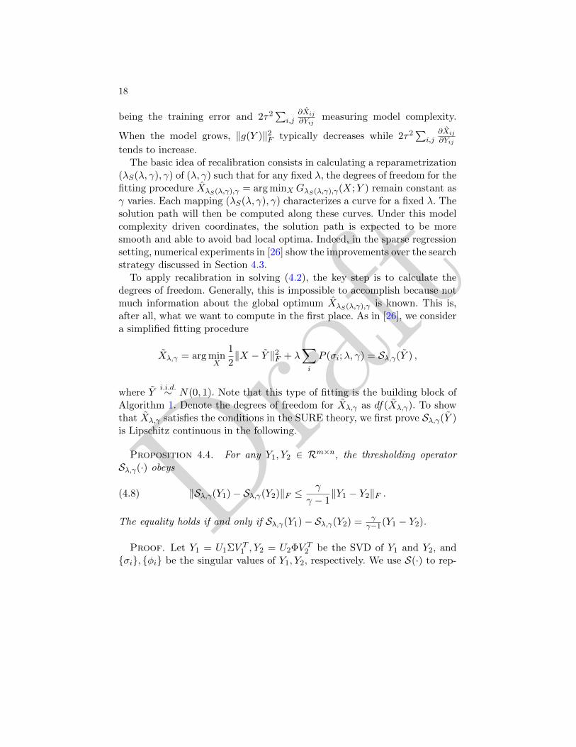
(λS(λ, γ), γ) of (λ, γ) such that for any fixed λ, the degrees of freedom for thefitting procedure XλS(λ,γ),γ = arg minX GλS(λ,γ),γ(X;Y ) remain constant asγ varies. Each mapping (λS(λ, γ), γ) characterizes a curve for a fixed λ. Thesolution path will then be computed along these curves. Under this modelcomplexity driven coordinates, the solution path is expected to be moresmooth and able to avoid bad local optima. Indeed, in the sparse regressionsetting, numerical experiments in [26] show the improvements over the searchstrategy discussed in Section 4.3.
To apply recalibration in solving (4.2), the key step is to calculate thedegrees of freedom. Generally, this is impossible to accomplish because notmuch information about the global optimum XλS(λ,γ),γ is known. This is,after all, what we want to compute in the first place. As in [26], we considera simplified fitting procedure
Xλ,γ = arg minX
1
2‖X − Y ‖2F + λ
∑i
P (σi;λ, γ) = Sλ,γ(Y ) ,
where Yi.i.d.∼ N(0, 1). Note that this type of fitting is the building block of
Algorithm 1. Denote the degrees of freedom for Xλ,γ as df(Xλ,γ). To showthat Xλ,γ satisfies the conditions in the SURE theory, we first prove Sλ,γ(Y )is Lipschitz continuous in the following.
Proposition 4.4. For any Y1, Y2 ∈ Rm×n, the thresholding operatorSλ,γ(·) obeys
(4.8) ‖Sλ,γ(Y1)− Sλ,γ(Y2)‖F ≤γ
γ − 1‖Y1 − Y2‖F .
The equality holds if and only if Sλ,γ(Y1)− Sλ,γ(Y2) = γγ−1(Y1 − Y2).
Proof. Let Y1 = U1ΣV T1 , Y2 = U2ΦV T
2 be the SVD of Y1 and Y2, andσi, φi be the singular values of Y1, Y2, respectively. We use S(·) to rep-

Draft
MATRIX COMPLETION VIA NON-CONVEX PROGRAMMING 19
resent Sλ,γ(·) and S(·) to denote Sγ(·;λ). Choosing L = [ γγ−1 ]2 yields
L‖Y1 − Y2‖2F − ‖S(Y1)− S(Y2)‖2F=
∑i
L(σ2i + φ2
i )− S(σi)2 − S(φi)
2 − 2Ltr(Y T1 Y2) + 2tr(S(Y1)TS(Y2))
=∑i
L(σ2i + φ2
i )− S(σi)2 − S(φi)
2
−2tr[(√LY1 − S(Y1))T (
√LY2 − S(Y2))]− 2tr[(
√LY1 − S(Y1))TS(Y2)]
−2tr[S(Y1)T (√LY2 − S(Y2))]
(b)
≥ ∑i
L(σ2i + φ2
i )− S(σi)2 − S(φi)
2
−2∑i
(√Lσi − S(σi))(
√Lφi − S(φi)) − 2
∑i
(√Lσi − S(σi))S(φi)
−2∑i
S(σi)(√Lφi − S(φi))
=∑i
[L(σi − φi)2 − (S(σi)− S(φi))2]
(c)
≥ 0 ,
where (b) holds by applying von Neumann’s trace inequality (A.1) and (c)follows from (4.5). Equality holds if and only if equality holds throughout(b) and (c). Equality can be achieved in (b) if and only if U1 = U2 andV1 = V2. Equality holds in (c) if and only if λ ≤ σi, φi ≤ λγ, implyingS(σi)−S(φi)
σi−φi = γγ−1 .
Consider now the set of matrices
F = Y ∈ Rm×n : Y is simple, of full rank, and no singular values
are equal to λ and λγ.
Since the singular values are continuous matrix functions, F is an openset. It is also not hard to see that the complement set Fc has Lebesguemeasure zero under the noisy setting (4.1). It is shown in [27] that Sλ,γ(Y )is differentiable over F , and∑
i,j
∂[Sλ,γ(Y )]ij∂Yij
=∑i
(S′γ(σi;λ) + |m− n|Sγ(σi;λ)
σi
)(4.9)
+2∑i 6=j
σiSγ(σi;λ)
σ2i − σ2
j
.

Draft
20
Thus [Sλ,γ(Y )]ij is weakly differentiable. Furthermore, Proposition 4.4implies
E∣∣∣∂[Sλ,γ(Y )]ij
∂Yij
∣∣∣ ≤ γ
γ − 1<∞
EYij [Sλ,γ(Y )]ij ≤ E1/2[Y 2ij ]E
1/2[S2λ,γ(Y )]ij ]
≤ C E1/2‖Sλ,γ(Y )− Sλ,γ(0)‖2F≤ C
γ
γ − 1E1/2‖Y ‖2F <∞ .
Thus, we have shown the following.
Proposition 4.5. The degrees of freedom of the fitting procedure Xλ,γ
obey
df(Xλ,γ) = E
∑i
(S′γ(σi;λ) + |m− n|Sγ(σi;λ)
σi
)+ 2
∑i 6=j
σiSγ(σi;λ)
σ2i − σ2
j
,
where the σi are the singular values of Y , with Yiji.i.d.∼ N(0, 1).
The degrees of freedom calculation in Proposition 4.5 involves a high-dimensional integral, which itself is a difficult problem. Instead, we use theMarchenko-Pastur law (A.2) to approximate it. Adopting the notation inAppendix A, it is not hard to verify that∑
i
(S′γ(σi;λ) + |m− n|Sγ(σi;λ)
σi
)+ 2
∑i 6=j
σiSγ(σi;λ)
σ2i − σ2
j
=
nEµn
S′γ(√x;λ) + |m− n|Sγ(
√x;λ)√x
+ 2n2Eµn
√xSγ(
√x;λ)
x− yI(x 6= y)
,
where x, yi.i.d.∼ µn. Let n
m = α, by the Marchenko-Pastur law, we have
df(Xλ,γ) ≈ nEµ
S′γ(√mx;λ) + |m− n|Sγ(
√mx;λ)√mx
(4.10)
+2n2Eµ
√mxSγ(
√mx;λ)
mx−myI(x 6= y)
,
where x, yi.i.d.∼ µ with parameter α. Note that (4.10) only requires two-
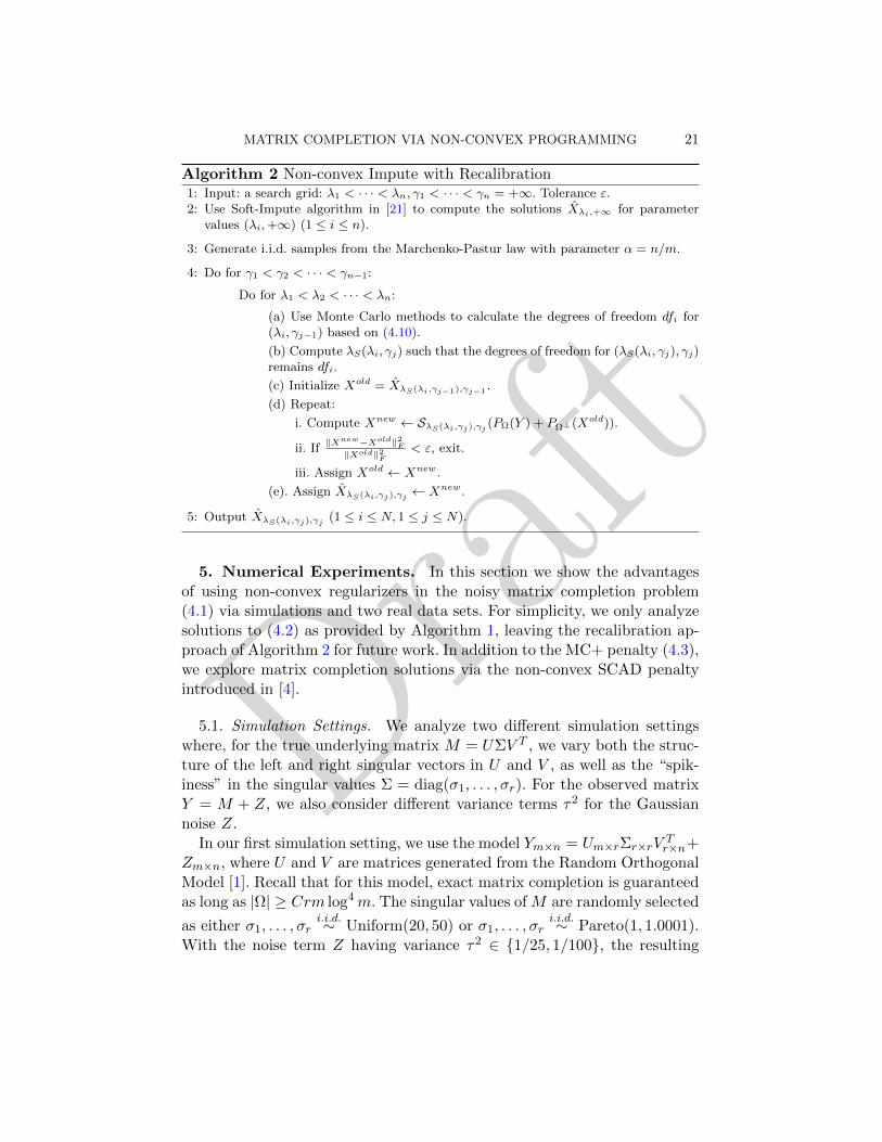
dimensional integrals which can be approximated by Monte Carlo methods.We now present Algorithm 2 with recalibration.
Draft
MATRIX COMPLETION VIA NON-CONVEX PROGRAMMING 21
Algorithm 2 Non-convex Impute with Recalibration1: Input: a search grid: λ1 < · · · < λn, γ1 < · · · < γn = +∞. Tolerance ε.2: Use Soft-Impute algorithm in [21] to compute the solutions Xλi,+∞ for parameter
values (λi,+∞) (1 ≤ i ≤ n).
3: Generate i.i.d. samples from the Marchenko-Pastur law with parameter α = n/m.
4: Do for γ1 < γ2 < · · · < γn−1:
Do for λ1 < λ2 < · · · < λn:
(a) Use Monte Carlo methods to calculate the degrees of freedom dfi for(λi, γj−1) based on (4.10).
(b) Compute λS(λi, γj) such that the degrees of freedom for (λS(λi, γj), γj)remains dfi.
(c) Initialize Xold = XλS(λi,γj−1),γj−1.
(d) Repeat:
i. Compute Xnew ← SλS(λi,γj),γj (PΩ(Y ) + PΩ⊥(Xold)).
ii. If‖Xnew−Xold‖2F‖Xold‖2
F< ε, exit.
iii. Assign Xold ← Xnew.
(e). Assign XλS(λi,γj),γj ← Xnew.
5: Output XλS(λi,γj),γj (1 ≤ i ≤ N, 1 ≤ j ≤ N).
5. Numerical Experiments. In this section we show the advantagesof using non-convex regularizers in the noisy matrix completion problem(4.1) via simulations and two real data sets. For simplicity, we only analyzesolutions to (4.2) as provided by Algorithm 1, leaving the recalibration ap-proach of Algorithm 2 for future work. In addition to the MC+ penalty (4.3),we explore matrix completion solutions via the non-convex SCAD penaltyintroduced in [4].
5.1. Simulation Settings. We analyze two different simulation settingswhere, for the true underlying matrix M = UΣV T , we vary both the struc-ture of the left and right singular vectors in U and V , as well as the “spik-iness” in the singular values Σ = diag(σ1, . . . , σr). For the observed matrixY = M + Z, we also consider different variance terms τ2 for the Gaussiannoise Z.
In our first simulation setting, we use the model Ym×n = Um×rΣr×rVTr×n+
Zm×n, where U and V are matrices generated from the Random OrthogonalModel [1]. Recall that for this model, exact matrix completion is guaranteedas long as |Ω| ≥ Crm log4m. The singular values of M are randomly selected
as either σ1, . . . , σri.i.d.∼ Uniform(20, 50) or σ1, . . . , σr
i.i.d.∼ Pareto(1, 1.0001).With the noise term Z having variance τ2 ∈ 1/25, 1/100, the resulting
Draft
22
matrix Y should have low “spikiness” (as defined in (2.8)) in the Uniformcase and the Pareto case when there is a single dominant sampled singularvalue, and higher “spikiness” when the observations sampled from the Paretoare clustered around one.
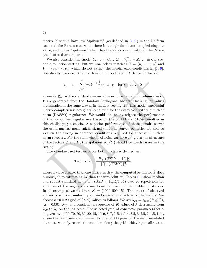
We also consider the model Ym×n = Um×rΣr×rVTr×n + Zm×n in our sec-
ond simulation setting, but we now select matrices U = (u1, · · · , ur) andV = (v1, · · · , vr) which do not satisfy the incoherence conditions in [1, 9].Specifically, we select the first five columns of U and V to be of the form
ui = vi =
4∑j=1
(−1)j−1 1
2ej+4(i−1) for i = 1, . . . , 5 ,
where (ei)mi=1 is the standard canonical basis. The remaining columns in U ,
V are generated from the Random Orthogonal Model. The singular valuesare sampled in the same way as in the first setting. For this model, successfulmatrix completion is not guaranteed even for the exact case with the nuclearnorm (LASSO) regularizer. We would like to investigate the performanceof the non-convex regularizers based on the SCAD and MC+ penalties inthis challenging scenario. A superior performance of these penalties overthe usual nuclear norm might signal that non-convex penalties are able toweaken the strong incoherence conditions required for successful nuclearnorm recovery. For the same choice of noise variance τ2, given the structureof the factors U and V , the spikiness αsp(Y ) should be much larger in thissetting.
The standardized test error for both models is defined as
Test Error =‖PΩ⊥(UΣV T − Y )‖2F‖PΩ⊥(UΣV T )‖2F
,
where a value greater than one indicates that the computed estimator Y doesa worse job at estimating M than the zero solution. Tables 1–2 show medianand robust standard deviation (RSD = IQR/1.34) over 20 repetitions forall three of the regularizers mentioned above in both problem instances.In all examples, we fix (m,n, r) = (1000, 500, 15). The set Ω of observedentries is sampled uniformly at random over the indices of the matrix. Wechoose a 20× 20 grid of (λ, γ) values as follows. We set λ20 = λmax(PΩ(Y )),λ1 = 0.001 · λ20, and construct a sequence of 20 values of λ decreasing fromλ20 to λ1 on the log scale. The selected grid of concavity parameters for γis given by 100, 70, 50, 30, 20, 15, 10, 9, 8, 7, 6, 5, 4.5, 4, 3.5, 3, 2.5, 2, 1.5, 1.1,where the last three are trimmed for the SCAD penalty. For each simulateddata set, we only record the solution along the grid achieving smallest test
Draft
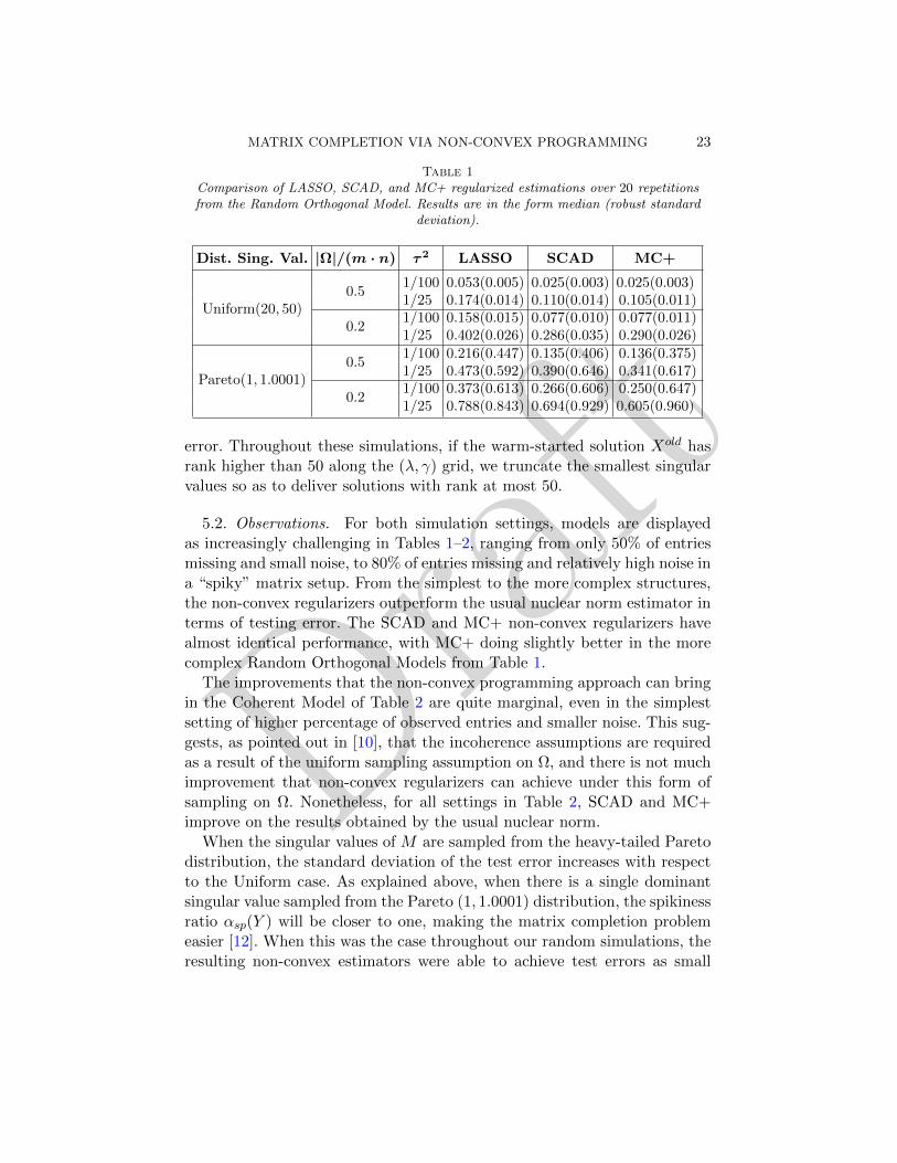
MATRIX COMPLETION VIA NON-CONVEX PROGRAMMING 23
Table 1Comparison of LASSO, SCAD, and MC+ regularized estimations over 20 repetitionsfrom the Random Orthogonal Model. Results are in the form median (robust standard
deviation).
Dist. Sing. Val. |Ω|/(m · n) τ2 LASSO SCAD MC+
Uniform(20, 50)0.5
1/100 0.053(0.005) 0.025(0.003) 0.025(0.003)1/25 0.174(0.014) 0.110(0.014) 0.105(0.011)
0.21/100 0.158(0.015) 0.077(0.010) 0.077(0.011)1/25 0.402(0.026) 0.286(0.035) 0.290(0.026)
Pareto(1, 1.0001)0.5
1/100 0.216(0.447) 0.135(0.406) 0.136(0.375)1/25 0.473(0.592) 0.390(0.646) 0.341(0.617)
0.21/100 0.373(0.613) 0.266(0.606) 0.250(0.647)1/25 0.788(0.843) 0.694(0.929) 0.605(0.960)
error. Throughout these simulations, if the warm-started solution Xold hasrank higher than 50 along the (λ, γ) grid, we truncate the smallest singularvalues so as to deliver solutions with rank at most 50.
5.2. Observations. For both simulation settings, models are displayedas increasingly challenging in Tables 1–2, ranging from only 50% of entriesmissing and small noise, to 80% of entries missing and relatively high noise ina “spiky” matrix setup. From the simplest to the more complex structures,the non-convex regularizers outperform the usual nuclear norm estimator interms of testing error. The SCAD and MC+ non-convex regularizers havealmost identical performance, with MC+ doing slightly better in the morecomplex Random Orthogonal Models from Table 1.
The improvements that the non-convex programming approach can bringin the Coherent Model of Table 2 are quite marginal, even in the simplestsetting of higher percentage of observed entries and smaller noise. This sug-gests, as pointed out in [10], that the incoherence assumptions are requiredas a result of the uniform sampling assumption on Ω, and there is not muchimprovement that non-convex regularizers can achieve under this form ofsampling on Ω. Nonetheless, for all settings in Table 2, SCAD and MC+improve on the results obtained by the usual nuclear norm.
When the singular values of M are sampled from the heavy-tailed Paretodistribution, the standard deviation of the test error increases with respectto the Uniform case. As explained above, when there is a single dominantsingular value sampled from the Pareto (1, 1.0001) distribution, the spikinessratio αsp(Y ) will be closer to one, making the matrix completion problemeasier [12]. When this was the case throughout our random simulations, theresulting non-convex estimators were able to achieve test errors as small
Draft
24
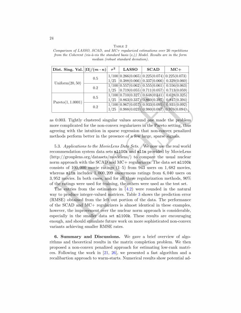
Table 2Comparison of LASSO, SCAD, and MC+ regularized estimations over 20 repetitionsfrom the Coherent (vis-a-vis the standard basis (ei)) Model. Results are in the form
median (robust standard deviation).
Dist. Sing. Val. |Ω|/(m · n) τ2 LASSO SCAD MC+
Uniform(20, 50)0.5
1/100 0.266(0.065) 0.225(0.074) 0.225(0.073)1/25 0.388(0.066) 0.337(0.066) 0.329(0.060)
0.21/100 0.557(0.062) 0.555(0.061) 0.556(0.063)1/25 0.719(0.055) 0.711(0.057) 0.713(0.059)
Pareto(1, 1.0001)0.5
1/100 0.710(0.327) 0.648(0.341) 0.628(0.325)1/25 0.863(0.337) 0.860(0.397) 0.847(0.394)
0.21/100 0.967(0.057) 0.933(0.095) 0.931(0.092)1/25 0.988(0.023) 0.980(0.087) 0.976(0.094)
as 0.003. Tightly clustered singular values around one made the problemmore complicated for the non-convex regularizers in the Pareto setting, thusagreeing with the intuition in sparse regression that non-convex penalizedmethods perform better in the presence of a few large, sparse signals.
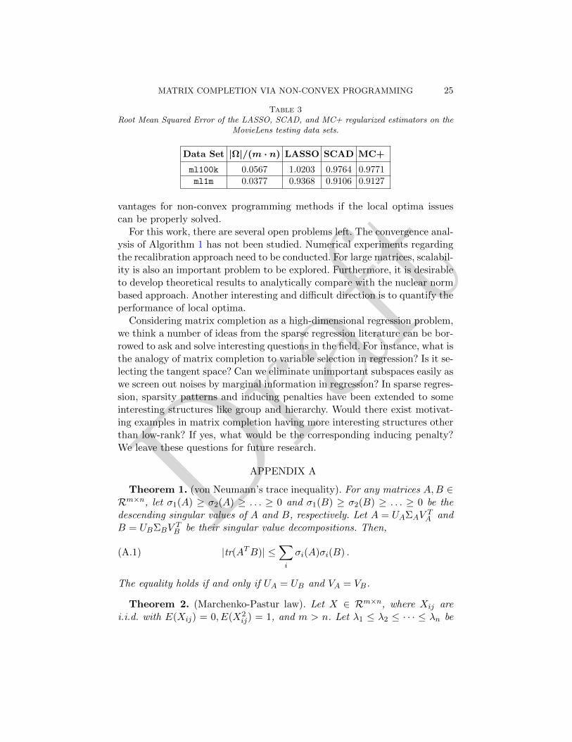
5.3. Applications to the MovieLens Data Sets. We now use the real worldrecommendation system data sets ml100k and ml1m provided by MovieLens(http://grouplens.org/datasets/movielens/) to compare the usual nuclearnorm approach with the SCAD and MC+ regularizers. The data set ml100kconsists of 100, 000 movie ratings (1–5) from 943 users on 1, 682 movies,whereas ml1m includes 1, 000, 209 anonymous ratings from 6, 040 users on3, 952 movies. In both cases, and for all three regularization methods, 90%of the ratings were used for training, the others were used as the test set.
The entries from the estimators in (4.2) were rounded in the naturalway to produce integer-valued matrices. Table 3 shows the prediction error(RMSE) obtained from the left out portion of the data. The performanceof the SCAD and MC+ regularizers is almost identical in these examples,however, the improvement over the nuclear norm approach is considerable,especially in the smaller data set ml100k. These results are encouragingenough, and should stimulate future work on more sophisticated non-convexvariants achieving smaller RMSE rates.
6. Summary and Discussions. We gave a brief overview of algo-rithms and theoretical results in the matrix completion problem. We thenproposed a non-convex penalized approach for estimating low-rank matri-ces. Following the work in [21, 26], we presented a fast algorithm and arecalibartion approach to warm-starts. Numerical results show potential ad-
Draft
MATRIX COMPLETION VIA NON-CONVEX PROGRAMMING 25
Table 3Root Mean Squared Error of the LASSO, SCAD, and MC+ regularized estimators on the
MovieLens testing data sets.
Data Set |Ω|/(m · n) LASSO SCAD MC+
ml100k 0.0567 1.0203 0.9764 0.9771ml1m 0.0377 0.9368 0.9106 0.9127
vantages for non-convex programming methods if the local optima issuescan be properly solved.
For this work, there are several open problems left. The convergence anal-ysis of Algorithm 1 has not been studied. Numerical experiments regardingthe recalibration approach need to be conducted. For large matrices, scalabil-ity is also an important problem to be explored. Furthermore, it is desirableto develop theoretical results to analytically compare with the nuclear normbased approach. Another interesting and difficult direction is to quantify theperformance of local optima.
Considering matrix completion as a high-dimensional regression problem,we think a number of ideas from the sparse regression literature can be bor-rowed to ask and solve interesting questions in the field. For instance, what isthe analogy of matrix completion to variable selection in regression? Is it se-lecting the tangent space? Can we eliminate unimportant subspaces easily aswe screen out noises by marginal information in regression? In sparse regres-sion, sparsity patterns and inducing penalties have been extended to someinteresting structures like group and hierarchy. Would there exist motivat-ing examples in matrix completion having more interesting structures otherthan low-rank? If yes, what would be the corresponding inducing penalty?We leave these questions for future research.
APPENDIX A
Theorem 1. (von Neumann’s trace inequality). For any matrices A,B ∈Rm×n, let σ1(A) ≥ σ2(A) ≥ . . . ≥ 0 and σ1(B) ≥ σ2(B) ≥ . . . ≥ 0 be thedescending singular values of A and B, respectively. Let A = UAΣAV
TA and
B = UBΣBVTB be their singular value decompositions. Then,
(A.1) |tr(ATB)| ≤∑i
σi(A)σi(B) .
The equality holds if and only if UA = UB and VA = VB.
Theorem 2. (Marchenko-Pastur law). Let X ∈ Rm×n, where Xij arei.i.d. with E(Xij) = 0, E(X2
ij) = 1, and m > n. Let λ1 ≤ λ2 ≤ · · · ≤ λn be

Draft
26
the eigenvalues of Sm = 1mX
TX. Define the random spectral measure
µn =1
n
n∑i=1
δλi .
Then, assuming n/m→ α ∈ (0, 1], we have
µn(·, ω)→ µ a.s.,
where µ is a deterministic measure with density
(A.2)dµ
dx=
√(α+ − x)(x− α−)
2παxI(α− ≤ x ≤ α+).
Here, α+ = (1 +√α)2, α− = (1−
√α)2.
REFERENCES
[1] E. Candes and B. Recht. (2009). Exact matrix completion via convex optimization.Foundations of Computational Mathematics, 9 717-772.
[2] ACM SIGKDD and Netflix. Proceedings of KDD Cup and Workshop, 2007.[3] R. Tibshirani. (1996). Regression shrinkage and selection via the lasso. Journal of
the Royal Statistical Society, Ser. B, 58 267-288.[4] J. Fan and R. Li. (2001). Variable selection via non concave penalized likelihood and
its oracle properties. Journal of the American Statistical Association, 96 1348-1360.[5] C. Zhang. (2010). Nearly unbiased variable selection under minimax concave penalty.
The Annals of Statistics, 38 894-942.[6] E. Candes and T. Tao. (2007). The Dantzig selector: statistical estimation when p
is much larger than n. The Annals of Statistics, 35 23132351.[7] E. Candes and Y. Plan. (2010). Matrix completion with noise. Proceedings of the
IEEE, 98, 925-936.[8] E. Candes and T. Tao. (2010). The power of convex relaxation: Near-optimal matrix
completion. IEEE Transactions on Information Theory, 56, 2053-2080.[9] B. Recht. (2011). A simpler approach to matrix completion. Journal of Machine
Learning Research, 12, 3413-3430.[10] Y. Chen, S. Bhojanapalli, S. Sanghavi and R. Ward. (2014). Coherent Matrix
Completion. Proceedings of the 31st International Conference on Machine Learning,2014.
[11] R. Keshavan, A. Montanari and S. Oh. (2010). Matrix completion from noisyentries. Journal of Machine Learning Research, 11, 2057-2078.
[12] S. Negahban and M. Wainwright. (2012). Restricted strong convexity andweighted matrix completion: optimal bounds with noise. Journal of Machine LearningResearch, 13, 1665-1697.
[13] S. Negahban, P. Ravikumar, M. Wainwright and B. Yu. (2012). A unified frame-work for high-dimensional analysis of M-estimators with decomposable regularizers.Statistical Science, 27, 538-557.
[14] E. Candes and Y. Plan. (2010). Tight oracle inequalities for low-rank matrix re-covery from a minimal number of noisy random measurements. IEEE Transactions onInformation Theory, 57(4), 2342-2359.

Draft
MATRIX COMPLETION VIA NON-CONVEX PROGRAMMING 27
[15] S. Negahban and M. Wainwright. (2011). Estimation of (near) low-rank matriceswith noise and high-dimensional scaling. The Annals of Statistics, 39, 1069-1097.
[16] A. Rohde and A. Tsybakov. (2011). Estimation of high-dimensional low-rank ma-trices. The Annals of Statistics, 39, 887-930.
[17] B. Recht, M. Fazel and P. Parrilo. (2010). Guaranteed minimum-rank solutionsof linear matrix equations via nuclear norm minimization. SIAM Review, 52, 471-501.
[18] J. Cai, E. Candes and Z. Shen. (2010). A singular value thresholding algorithm formatrix completion. SIAM Journal on Optimization, 20, 1956-1982.
[19] A. Beck and M. Teboulle. (2009). A fast iterative shrinkage-thresholding algorithmfor linear inverse problems. SIAM Journal on Imaging Sciences, 2, 183-202.
[20] S. Ma, D. Goldfarb and L. Chen. (2011). Fixed point and Bregman iterativemethods for matrix rank minimization. Math.Program., Ser. A 128, 321-353.
[21] R. Mazumder, T. Hastie and R. Tibshirani. (2010). Spectral regularization algo-rithms for learning large incomplete matrices. Journal of Machine Learning Research,11, 2287-2322.
[22] E. Hale, W. Yin and Y. Zhang. (2007). A fixed-point continuation method for ell1-regularized minimization with applications to compressed sensing. Technical Report,CAAM TR07-07.
[23] D. Hunter and R. Li. (2005). Variable selection using MM algorithms. The Annalsof Statistics, 33, 1617-1642.
[24] M. Jaggi and M. Sulovsky. (2010). A simple algorithm for nuclear norm regular-ized problems. Proceedings of the 27th International Conference on Machine Learning,2010.
[25] E. Hazan. (2008). Sparse approximation solutions to semidefinite programs. LATIN,pp. 306-316.
[26] R. Mazumder, J. Friedman and T. Hastie. (2011). SparseNet: Coordinate descentwith nonconvex penalties. Journal of the American Statistical Association, 106 ,1125-1138.
[27] E. Candes, C. Sing-Long and J. Trzasko. (2013). Unbiased risk estimates for sin-gular value thresholding and spectral estimators. IEEE Transactions on Signal Pro-cessing, 61, 4643-4657.
[28] R. Horn and C. Johnson. (1985). Matrix Analysis. Cambridge University Press,Cambridge.
[29] A. Lewis. (1995). The convex analysis of unitarily invariant matrix functions. Journalof Convex Analysis, 2, 173-183.
[30] B. Efron. (2004). The estimation of prediction error: Covariance penalties and cross-validation (with discussion). J. Amer. Statist. Assoc. 99, 619-632.
[31] C. Stein. (1981). Estimation of the mean of a multivariate normal distribution. TheAnnals of Statistics, 9, 1135-1151.
[32] B. Efron, T. Hastie, I. Jonstone and R. Tibshirani. (2004). Least angle regression.The Annals of Statistics, 32, 407-499.


![Convex Coupled Matrix and Tensor Completion …arXiv:1705.05197v2 [stat.ML] 14 Jun 2018 Convex Coupled Matrix and Tensor Completion Kishan Wimalawarne Bioinformatics Center, Institute](https://img.pdfslide.us/doc/110x75/5e60bc431036ec2ab9156b98/convex-coupled-matrix-and-tensor-completion-arxiv170505197v2-statml-14-jun.jpg)

![y Applied and Computational Mathematics, Caltech, Pasadena, CA … · 2008. 5. 29. · Exact Matrix Completion via Convex Optimization Emmanuel J. Cand esyand Benjamin Recht] yApplied](https://img.pdfslide.us/doc/110x75/60bad4ab305ad875bf2f7a83/y-applied-and-computational-mathematics-caltech-pasadena-ca-2008-5-29-exact.jpg)


![Exact Matrix Completion via Convex Optimizationcandes/papers/MatrixCompletion.pdf · Exact Matrix Completion via Convex Optimization Emmanuel J. Cand esyand Benjamin Recht] yApplied](https://img.pdfslide.us/doc/110x75/5b3ffeab7f8b9a4b3f8cc56a/exact-matrix-completion-via-convex-optimization-candespapersmatrixcompletionpdf.jpg)