© Faculty of Mechanical Engineering, Belgrade. All rights reserved FME Transactions (2019) 47, 183-189 183

Received: September 2018, Accepted: November 2018

Correspondence to: Mato Perić

Bestprojekt Ltd., Petrovaradinska 7

10000, Zagreb, Croatia

E-mail: mato.peric@fsb.hr

doi:10.5937/fmet1901183P

Mato Perić

Bestprojekt Ltd. Petrovaradinska 7

10000 Zagreb Croatia

Zdenko Tonković

Faculty of Mechanical Engineering and Naval Architecture

Ivana Lučića 5 10000 Zagreb

Croatia

Katarina S. Maksimović

Research Associate City Administration of the City of Belgrade

11000 Belgrade

Dragi Stamenković

Research Assistant Visoka brodarska škola

akademskih studija Bulevar vojvode Mišića 37

11000 Belgrade

Numerical Analysis of Residual Stresses in a T-Joint Fillet Weld Using a Submodeling Technique

A submodeling technique is applied in the framework of this study on a T-

joint fillet weld example in order to check finite element mesh sensitivity as

well as to obtain more accurate temperatures, displacements and residual

stress fields in the weld and its vicinity where the temperature and stress

gradients are very high. The submodeling procedure of the welding

process is demonstrated step-by-step. The obtained results of the

temperature, residual stress and displacement distributions correspond

very well with the experimental measurements and analytical solutions

from the literature.

Keywords Submodeling, T-joint fillet weld, finite element analysis,

residual stress, welding distortion, Abaqus, welding simulation

1. INTRODUCTION

Welding is one of the most frequently used engineering

methods of joining structural components in many

industrial fields. Large localised heat input during

welding and subsequent rapid cooling of melted

materials can have as a harmful consequence permanent

residual stresses and geometrical imperfection occur–

rences in the welded structures. Such geometrical

imperfections can cause serious problems during

structure assembly, while high tensile residual stresses

in combination with the workload can have a

detrimental impact on its integrity and life-time [1-4].

The elimination of these consequences by using

post-weld thermal or mechanical treatments requires

extended production time and causes additional finan–

cial expenses. For these reasons, it is highly desirable to

know the magnitude of residual stresses and distortions

in the structure as early as the design phase. Due to the

rapid progress of computer technology in recent

decades, the numerical calculations of residual stresses

and distortions have become an unavoidable tool for

predicting these phenomena by shifting expensive

experiments to computationally based procedures [5-9].

The main problem that exists here is the long-time

duration of numerical simulations in models with a large

number of finite elements.

To overcome this problem, there are many suggested

solutions in the literature. Shen and Chen [10], Rong et

al. [11], Perić et al. [12,13] and Rezaei et al. [14]

proposed various solutions based on coupling shell and

three-dimensional finite elements that significantly

reduce the calculation time. Huang and Murakawa [15]

developed in their study a dynamic mesh refining method

to speed up the calculation process that significantly

reduces the number of freedom in a finite element model.

Most of the suggested solutions above are related to the

reduction of calculation time primarily in the processing

phase. For time-reduction in the pre-processing phase,

there are only limited data in the literature provided. In

that sense, Seleš et al. [16] and Elmesalamy et al. [17]

used Abaqus Plug-in Software (AWI) to speed-up the

modeling of thermal loads and boundary conditions that

greatly reduce the model preparation time. Furthermore,

it is well known that the size of finite element meshes has

a great influence on the result accuracy and compu–

tational time, so that the finite element calculations with

refined meshes have to be done several times in a row

[18,19] before tackling the numerical simulation of the

welding process. This approach is often unsuitable for

engineering applications, especially for models with a

large number of finite elements, since it consumes too

much computational time. For this reason, the submo–

deling technique in this study which is based on global-

local transition is applied to check the finite element

mesh sensitivity as well as to obtain finer residual stress

and displacement distribution in the area of interest.

In the submodeling technique, the results from the

global model are interpolated onto the nodes on the

appropriate parts of the submodel boundary. As the

submodel region has a finer mesh, the submodel can

provide an accurate, detailed solution. Unlike a large

number of papers where the submodeling capability is

used in the mechanical analysis to obtain a distribution of

high stresses caused by geometric discontinuities [20], a

very limited number of studies have been reported in the

area dealing with submodeling techniques in the

thermomechanical analysis of welding processes [21, 22].

This paper is organized as follows: Section 2 provides

a brief description of the submodeling application on a

welding simulation process. The numerical model is

presented in Section 3. Section 4 gives a comparison of

temperatures, deflections and residual stresses obtained

using the submodeling technique with the results from

184 ▪ VOL. 47, No 1, 2019 FME Transactions

literature as well as with the results from the global

model. Finally, some concluding remarks are given in the

last section.

2. WELDING SIMULATION USING SUBMODELING TECHNIQUE

The principle of the submodeling technique for the

simulation of the welding process consists of four steps

and it is given in Fig. 1. In the first step, a heat transfer

analysis is done to obtain temperature-time history at

each node on the global model. The obtained thermal

field is then used as a thermal load in the mechanical

analysis in the second step to obtain residual stresses

and displacements. The obtained temperature histories

on the global model boundary nodes are then transferred

as driven variables from the global model boundaries

onto the submodel ones in the third step. Finally, in the

fourth step, the obtained submodel temperature histories

from the third step are then applied as a thermal load in

the fourth step, while the displacement obtained from

the global model boundaries from the second step are

simultaneously used as driven variables. Since the

submodel dimensions are usually significantly less than

the global ones, this allows for much denser finite

element meshes (mesh-2) in the submodel analysis.

3. NUMERICAL MODEL

To verify the submodel technique, a T-joint fillet weld

with experimentally measured plate deflections is taken

from the literature [23]. The dimensions of the welded

model with mechanical restraints are given in Fig. 2. A

two single pass MAG welding with no time-gap

between the weld passes is used. The welding

parameters are as follows: welding voltage U = 29 V,

welding current I = 270 A, welding speed v = 400

mm/min and angle of torch α = 45°. The plates are made

of SM400A carbon steel which chemical compositions

are given in Table 1, while its thermal and mechanical

properties are given in Figs. 3 and 4.

Table 1. Chemical composition of SM400A steel [23]

Elements C Si Mn P S

Mass % 0.23 - 0.56 <0.0035 <0.0035

0

0.2

0.4

0.6

0.8

1

1.2

1.4

0 250 500 750 1000 1250 1500

Temperature [°C]

Therm

al pro

pert

ies

Thermal conductivity

Specific heat

Density

(104

kgm-3

)

(102 Wm

-1K

-1)

(103

Jkg-1

K-1

)

Figure 3. Thermal properties of SM400A steel [24]

0

50

100

150

200

250

300

350

0 250 500 750 1000 1250 1500

Temperature [°C]

Mechanic

al pro

pert

ies

Yield stress (MPa)Modulus of elasticity (GPa)Thermal expansion coefficient (1/°C)Poisson's ratio

(10-7

)

(10-2

)

Figure 4. Mechanical properties of SM400A steel [24]

Globa model ( mesh-1)Thermal analysis

Submodel ( mesh-2)

Global model ( mesh-1)

Global.odb

Driven variables

Global.odbThermal field

1

2

3

4

1storder DC3D8 elements

Global.odb

Driven variables

Thermal analysis

order DC3D8 elements1st

Submodel.odbThermal field

Mechanical analysis

order C3D8I elements1st

Mechanical analysisSubmodel ( mesh-2)order C3D8I elements1st

( temperatures)

( displacements)

Figure 1. Sheme of welding submodeling technique

x

y

z

300

5009

9

6

weld

500

A 250

250

first

weld

second

weld

mechanical restraint in x, y and z direction

mechanical restraint in y and z direction

mechanical restraint in y direction

6 second

weld

firs

tw

eld

E

A

DC

Section A-A

45°

*dimensions in milimeters

C D

99

217

20

Submodel

Global model

F

G

Figure 2. Geometry of T-joint welded plates

FME Transactions VOL. 47, No 1, 2019 ▪ 185

As it can be seen in Fig. 1, a sequentially coupled

numerical simulation of welding process is applied in

this study. It means that a full analysis consists of two

independent analyses: thermal and mechanical ones. In

the thermal analysis, the governing equation for

transient nonlinear heat transfer is given in the form of

x y y

T T T Tk k k Q C

x x y y z z tρ

∂ ∂ ∂ ∂ ∂ ∂ ∂ + + + =

∂ ∂ ∂ ∂ ∂ ∂ ∂ (1)

where kx, ky, and kz are the thermal conductivities in the

x, y and z directions, respectively; T is the temperature;

Q is the heat input; ρ is the material density; C is the

specific heat capacity; and t is the time, respectively. A

general solution of Eq. (1) can be obtained by intro–

ducing the following initial and boundary conditions

0( , , ,0) ( , , )T x y z T x y z= (2)

( ) ( ) 0

x x y y z z s

c r r

T T Tk N k N k N q

x y z

h T T h T T∞

∂ ∂ ∂+ + + +

∂ ∂ ∂

+ − + − =

(3)

where Nx, Ny, and Nz are the direction cosine of the

normal to the boundary; hc and hr are the convection and

radiation heat transfer coefficients, respectively; qs

denotes the boundary heat flux; Tr denotes the tempe–

rature of radiation; and T∞ represents the ambient

temperature. Radiation heat loses can be expressed by

the following equation

2 2( )( )r r rh F T T T Tσε= + + (4)

where σ = 5.67 × 10-8 Jm-2K-4 denotes the Stefan–

Boltzmann constant, ε is the surface emissivity factor,

and F is the configuration factor. The total heat input

applied to the weld is given by:

H

UIQ

V

η= (5)

where η represents the heat input efficiency, I is welding

current, U is the arc voltage, and VH is the volume of the

activated set of finite elements. In the thermal analysis

of this study, the filler metal addition is simulated by

element birth and death technique. The segmented heat

flux with uniformly distributed Q = 5.22 × 1010 Jm-3s-1

per weld volume is applied and it is calculated according

to Eq. (5). Additionally, the following thermal boundary

conditions are assumed: convective heat transfer

coefficient k = 10 Wm-2K-1, emissivity of plate surfaces

ε = 0.9 and the weld process efficiency η = 80%. In the

thermal analysis, three-dimensional 8-node solid

DC3D8 elements are used.

To speed up-the simulation process, the mechanical

analysis is conduced simultaneously in one step, without

using the element and birth technique [25]. In the me–

chanical analysis, an elastic-perflectly plastic behavior

of the material is assumed. The same finite element

mesh that consists of a 19,188 finite element mesh (Fig.

5) as in the thermal analysis is used, with only the finite

element type being converted to C3D8I. The influence

of the metal phase transformation is not considered in

this study because its influence on the residual stress

field and deformations can be neglected in low-carbon

steel [26,27]. Creep material behavior is also neglected

because the thermal cycles during the welding are of

very short time duration. In doing so, the total strain

increments can be decomposed into three components:

{ } { } { }total e p thd d d dε ε ε ε= + + (6)

where {dεe}, {dε

p} and {dεth} are elastic, plastic and

thermal strain increments, respectively. Furthermore, in

all numerical simulations it is assumed that the base

metal and weld filler metal have the same thermal and

mechanical properties.

The mesh sensitivity of the full (global) model,

using the submodeling technique, is conducted on a

small volume, 217 mm × 99 mm × 20 mm, in the weld

and its vicinity where the temperature gradients are very

high. The location of the submodeling is shown in Figs.

2 and 5. It should be noted that the submodel mesh is

created with a very high dense finite element mesh. It is

clear, that the use of such dense finite element meshes

in the full global model can lead to thermal and mecha–

nical simulations which are computationally unsolvable.

The dimensions of the submodel and the number of

finite elements of the submodel are given in Table 2.

Additionally, a comparison is given between the

finite element number of the submodel and the equi–

valent volume of the same dimensions in the full global

model. All numerical simulations in this study are

performed by using the Abaqus/Standard software.

Global model

Submodel

Figure 5. Typical finite element mesh

Table 2. Dimensions and number of finite elements of submodel and equivalent part of global model

Name Dimensions Number of finite

elements

Global model* 217 mm × 99 mm ×

20 mm

1092

Submodel 217 mm × 99 mm ×

20 mm

22,320

(*equivalent volume to submodel volume)

4. RESULTS AND DISCUSSION

The temperature time-history of node E which is located

at the bottom surface of the horizontal plate (Fig. 2) for

186 ▪ VOL. 47, No 1, 2019 FME Transactions

the first 150 s after the beginning of the welding process

is given in Fig. 6. It is obvious that the temperature

time-history of the global model and submodel are

almost identical. More detailed peak temperature com–

parisons after the first and second weld pass are given in

Figs. 7 and 8, respectively. The peak temperatures of the

global model are 1% higher than in the submodel.

Further submodeling with meshes of higher density has

no additional influence on the submodel temperatures,

and it can be stated that the temperatures converge.

Keeping this in mind, it can be concluded that the global

mesh for the thermal analysis is properly designed.

The obtained longitudinal residual stress (stress in

the welding direction) at the middle plane of the ho–

rizontal plate along line C-D (Fig. 2) for the global

model and submodel is shown in Fig 9. Here, it is seen

that the longitudinal residual stress of the global model

and submodel coincide very well.

0

100

200

300

400

500

600

0 25 50 75 100 125 150Time [s]

Tem

pera

ture

[°C

]

Global model

Submodel

Figure 6. Temperature time-history at node E (Fig 2.) of global model and submodel

300

320

340

360

380

400

420

440

460

35 40 45 50 55

Time [s]

Tem

pera

ture

[°C

]

Global model

Submodel

Figure 7. Peak temperature of global model and submodel after first weld pass

480

490

500

510

520

530

540

550

560

115 120 125 130Time [s]

Tem

pera

ture

[°C

]

Global model

Submodel

Figure 8. Peak temperature of global model and submodel after second weld pass

Due to a lack of experimental measurements in [23],

the calculated longitudinal stresses are compared with

the widely used analytical solution [28]. The peak

longitudinal residual stresses is about 5% higher than

the analytical solution. The width of the numerically

calculated tensile longitudinal stress zone is 66.3 mm

and is the same for the global model and submodel,

while the analytical calculated tensile residual stress

zone is 69.2 mm. The full field longitudinal residual

stress distribution of the T-joint welded plates along C-

D line (Fig. 2), for the global model and submodel is

given in Fig. 10.

-100

-50

0

50

100

150

200

250

300

350

150 200 250 300 350

x - Coordinate [mm]

Resid

ual str

ess [

MP

a]

GlobalmodelSubmodel

Analytical[28]

Figure 9. Longitudinal residual stress distribution of global model and submodel at middle surface of horizontal plate

along C-D line shown in Fig. 2

Figure 10. Full field longitudinal residual stress distribution of T-joint welded plates along C-D line shown in Fig. 2: a) global model, b) submodel

The calculated transversal residual stress (stress

parpendicular to the welding direction) at the middle

plane of the horizontal plate along line C-D (Fig. 2) for

both, global model and submodel is shown in Fig 11. As

FME Transactions VOL. 47, No 1, 2019 ▪ 187

in the longitudinal stress comparison, it is noticeable

that the longitudinal residual stress of the global model

and submodel coincide very well. The full field

transversal residual stress distribution of the T-joint

welded plates along C-D line (Fig. 2), for the global

model and submodel is given in Fig. 12. Additionaly,

the thickness of the transversal residual stress profile

along F-G line (Fig. 2) is shown in Fig. 13. Here, node F

is located on the lower surface of the horizontal plate,

and node G on the lower surface of the horizontal plate.

The obtained average through the thickness of the

transverse residual stress difference between the global

model and submodel is under 10%.

0

10

20

30

40

50

60

70

80

150 200 250 300 350x - Coordinate [mm]

Resid

ual str

ess [

MP

a]

Global model

Submodel

Figure 11. Transversal residual stress distribution of global model and submodel at middle surface of horizontal plate along C-D line shown in Fig. 2

Figure 12. Full field transversal residual stress distribution of T-joint welded plates along C-D line shown in Fig. 2: a) global model, b) submodel

A comparison between the vertical deflections of

the horizontal plate at the middle surface along C-D

(Fig. 2) between the global model and submodel is

given in Fig. 14, while their full field comparison is

given in Fig. 15. As it can be seen, the calculated

vertical displacement of the global model and submodel

correspond very well.

-10

0

10

20

30

40

50

60

70

80

90

0 1 2 3 4 5 6 7 8 9y - Coordinate [mm]

Resid

ual str

ess [

MP

a]

Submodel

Global model

Figure 13. Through thickness transversal residual stress profile along F-G line shown Fig. 2

-6.0

-5.5

-5.0

-4.5

-4.0

-3.5

-3.0

150 200 250 300 350

x - Coordinate [mm]

Deflection [m

m]

Experimental [23]

Global model

Submodel

Figure 14. Deflection distributions of horizontal plate at middle surface along C-D line shown in Fig. 2

Figure 15. Full vertical deflection field of T-joint welded plates along C-D line shown in Fig. 2: a) global model, b) submodel

188 ▪ VOL. 47, No 1, 2019 FME Transactions

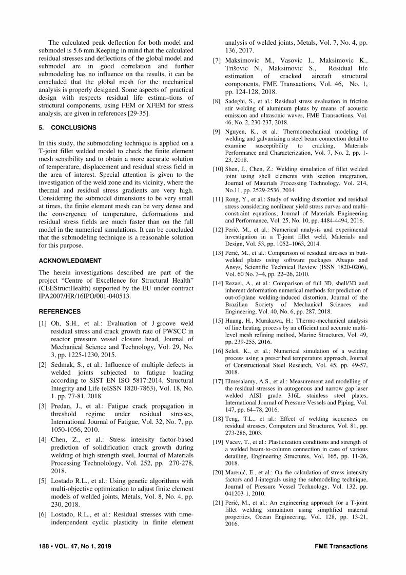
The calculated peak deflection for both model and

submodel is 5.6 mm.Keeping in mind that the calculated

residual stresses and deflections of the global model and

submodel are in good correlation and further

submodeling has no influence on the results, it can be

concluded that the global mesh for the mechanical

analysis is properly designed. Some aspects of practical

design with respects residual life estima–tions of

structural components, using FEM or XFEM for stress

analysis, are given in references [29-35]. 5. CONCLUSIONS

In this study, the submodeling technique is applied on a

T-joint fillet welded model to check the finite element

mesh sensibility and to obtain a more accurate solution

of temperature, displacement and residual stress field in

the area of interest. Special attention is given to the

investigation of the weld zone and its vicinity, where the

thermal and residual stress gradients are very high.

Considering the submodel dimensions to be very small

at times, the finite element mesh can be very dense and

the convergence of temperature, deformations and

residual stress fields are much faster than on the full

model in the numerical simulations. It can be concluded

that the submodeling technique is a reasonable solution

for this purpose.

ACKNOWLEDGMENT

The herein investigations described are part of the

project “Centre of Excellence for Structural Health”

(CEEStructHealth) supported by the EU under contract

IPA2007/HR/16IPO/001-040513.

REFERENCES

[1] Oh, S.H., et al.: Evaluation of J-groove weld

residual stress and crack growth rate of PWSCC in

reactor pressure vessel closure head, Journal of

Mechanical Science and Technology, Vol. 29, No.

3, pp. 1225-1230, 2015.

[2] Sedmak, S., et al.: Influence of multiple defects in

welded joints subjected to fatigue loading

according to SIST EN ISO 5817:2014, Structural

Integrity and Life (eISSN 1820-7863), Vol. 18, No.

1. pp. 77-81, 2018.

[3] Predan, J., et al.: Fatigue crack propagation in

threshold regime under residual stresses,

International Journal of Fatigue, Vol. 32, No. 7, pp.

1050-1056, 2010.

[4] Chen, Z., et al.: Stress intensity factor-based

prediction of solidification crack growth during

welding of high strength steel, Journal of Materials

Processing Technolology, Vol. 252, pp. 270-278,

2018.

[5] Lostado R.L., et al.: Using genetic algorithms with

multi-objective optimization to adjust finite element

models of welded joints, Metals, Vol. 8, No. 4, pp.

230, 2018.

[6] Lostado, R.L., et al.: Residual stresses with time-

indenpendent cyclic plasticity in finite element

analysis of welded joints, Metals, Vol. 7, No. 4, pp.

136, 2017.

[7] Maksimovic M., Vasovic I., Maksimovic K.,

Trišovic N., Maksimovic S., Residual life

estimation of cracked aircraft structural

components, FME Transactions, Vol. 46, No. 1,

pp. 124-128, 2018.

[8] Sadeghi, S., et al.: Residual stress evaluation in friction

stir welding of aluminum plates by means of acoustic

emission and ultrasonic waves, FME Transactions, Vol.

46, No. 2, 230-237, 2018.

[9] Nguyen, K., et al.: Thermomechanical modeling of

welding and galvanizing a steel beam connection detail to

examine susceptibility to cracking, Materials

Performance and Characterization, Vol. 7, No. 2, pp. 1-

23, 2018.

[10] Shen, J., Chen, Z.: Welding simulation of fillet welded

joint using shell elements with section integration,

Journal of Materials Processing Technology, Vol. 214,

No.11, pp. 2529-2536, 2014

[11] Rong, Y., et al.: Study of welding distortion and residual

stress considering nonlinear yield stress curves and multi-

constraint equations, Journal of Materials Engineering

and Performance, Vol. 25, No. 10, pp. 4484-4494, 2016.

[12] Perić, M., et al.: Numerical analysis and experimental

investigation in a T-joint fillet weld, Materials and

Design, Vol. 53, pp. 1052–1063, 2014.

[13] Perić, M., et al.: Comparison of residual stresses in butt-

welded plates using software packages Abaqus and

Ansys, Scientific Technical Review (ISSN 1820-0206),

Vol. 60 No. 3–4, pp. 22–26, 2010.

[14] Rezaei, A., et al.: Comparison of full 3D, shell/3D and

inherent deformation numerical methods for prediction of

out-of-plane welding-induced distortion, Journal of the

Brazilian Society of Mechanical Sciences and

Engineering, Vol. 40, No. 6, pp. 287, 2018.

[15] Huang, H., Murakawa, H.: Thermo-mechanical analysis

of line heating process by an efficient and accurate multi-

level mesh refining method, Marine Structures, Vol. 49,

pp. 239-255, 2016.

[16] Seleš, K., et al.; Numerical simulation of a welding

process using a prescribed temperature approach, Journal

of Constructional Steel Research, Vol. 45, pp. 49-57,

2018.

[17] Elmesalamy, A.S., et al.: Measurement and modelling of

the residual stresses in autogenous and narrow gap laser

welded AISI grade 316L stainless steel plates,

International Journal of Pressure Vessels and Piping, Vol.

147, pp. 64–78, 2016.

[18] Teng, T.L., et al.: Effect of welding sequences on

residual stresses, Computers and Structures, Vol. 81, pp.

273-286, 2003.

[19] Vacev, T., et al.: Plasticization conditions and strength of

a welded beam-to-column connection in case of various

detailing, Engineering Structures, Vol. 165, pp. 11-26,

2018.

[20] Marenić, E., et al.: On the calculation of stress intensity

factors and J-integrals using the submodeling technique,

Journal of Pressure Vessel Technology, Vol. 132, pp.

041203-1, 2010.

[21] Perić, M., et al.: An engineering approach for a T-joint

fillet welding simulation using simplified material

properties, Ocean Engineering, Vol. 128, pp. 13-21,

2016.

FME Transactions VOL. 47, No 1, 2019 ▪ 189

[22] Bonifaz, E.A., Submodeling simulations in fusion welds,

Journal of Multiscale Modelling, Vol. 4, No. 4, pp. 1-14,

2012.

[23] Deng, D., et al.: Determination of welding deformation in

fillet-welded joint by means of numerical simulation and

comparison with experimental measurements, Journal of

Materials Processing Technology, Vol. 183, No. 2-3, pp.

219–225, 2007.

[24] Gannon, L., et al.: Effect of welding sequence on residual

stress and distortion in flat-bar stiffened plates, Marine

Structures, Vol. 23, No. 3, pp. 385–404, 2010.

[25] Perić. M., et al.: A simplified engineering method for a

T-joint welding simulation, Thermal Science, Vol 22, No.

3, pp. S867-S873, 2018.

[26] Deng, D., FEM prediction of welding residual stress and

distortion in carbon steel considering phase

transformation effects, Materials and Design, Vol. 30,

No. 2, pp. 359-366, 2009.

[27] Knoedel, P., et al.: Practical aspects of welding residual

stress simulation, Journal of Constructional Steel

Research, Vol. 132, pp. 83-96, 2017.

[28] Chen, B.Q., Soares G.C.: Effects of plate configurations

on the weld induced deformations and strength of fillet-

welded plates, Marine Structures, Vol. 50, pp. 243-259,

2016.

[29] Grbovic, A., Rasuo, B.: FEM based fatigue crack growth

predictions for spar of light aircraft under variable

amplitude loading, Engineering Failure Analysis, Vol.

26, pp. 50–64, 2012.

[30] Boljanovic S., Maksimovic S., Computational mixed

mode failure analysis under fatigue loadings with

constant amplitude and overload, ENGINEERING

FRACTURE MECHANICS, (2017), vol. 174, pp. 168-

179.

[31] Petrašinović, N., Petrašinović, D., Rašuo B., Milković D.:

Aircraft Duraluminum Wing Spar Fatigue Testing, FME

Transactions, Vol. 45, No. 4, pp 531-536, 2017.

[32] Petrašinović, D., Rašuo, B., Petrašinović, N.: Extended

finite element method (XFEM) applied to aircraft

duralumin spar fatigue life estimation, Technical Gazette,

Vol. 19(3), pp. 557-562, 2012.

[33] Rasuo, B., Grbovic, A., Petrasinovic, D.: Investigation of

fatigue life of 2024-T3 aluminum spar using Extended

Finite Element Method (XFEM), SAE International

Journal of Aerospace, 6 (2013-01-2143), pp 408-416,

2013.

[34] Grbovic A., Rasuo B.: Use of modern numerical methods

for fatigue life predictions, in: Recent Trends in Fatigue

Design, Branco R. (Ed.), Nova Science Publishers, New

York. Chapter 2., pp.31-75, 2015.

[35] Kastratović, G., Vidanović, N., Grbović, A., Rašuo, B.:

Approximate determination of stress intensity factor for

multiple surface cracks, FME Transactions, Vol. 46, No.

1, pp 41-47, 2018.

НУМЕРИЧКА АНАЛИЗА ЗАОСТАЛИХ

НАПОНА У ЗАВАРЕНИМ ПЛОЧАМА У

ОБЛИКУ Т-СПОЈА КОРИШЋЕЊЕМ

ТЕХНИКЕ ПОДМОДЕЛИРАЊА

М. Перић, З. Тонковић, К.С. Максимовић,

Д. Стаменковић

У оквиру овoг рада примењена је техника

подмоделирања на примеру заварених плоча у

облику Т-споја, како би се проверила осетљивост

мреже са коначним елементима, као и да се добију

прецизније расподеле температура, померања и

поља заосталих напона у завареном споју и у

његовој околини где су градијенти температуре и

напона веома високи. Процедура субмоделирања

процеса заваривања приказана је корак по корак.

Добијени резултати расподеле температуре,

заосталих напона и померања веома добро се слажу

са експерименталним мерењима и аналитичким

решењима из литературе.