Embed Size (px)
Citation preview


MATLAB Tutorial

CONTENTS
Quick Start
Language Fundamentals
Mathematics
Graphics
Programming

MATLAB Tutorial
Matrices and Arrays
Array Creation
To create an array with four elements in a single row, separate
the elements with either a comma (,) or a space.
a = [1 2 3 4]
This type of array is a row vector.
To create a matrix that has multiple rows, separate the rows with
semicolons.
a = [1 2 3; 4 5 6; 7 8 10]

Matrices and Arrays
Another way to create a matrix is to use a function, such as ones, zeros, or rand.
For example, create a 5-by-1 column vector of zeros.
z = zeros(5,1)
For example, create a 1-by-5 column vector of zeros.
z = zeros(1,5)
MATLAB allows you to process all of the values in a matrix using a single arithmetic operator or function.
a + 10

Matrices and Arrays
Matrix and Array Operations
MATLAB allows you to process all of the values in a matrix using a single arithmetic operator or function.
a + 10
ans = 3×3
11 12 13
14 15 16
17 18 20
sin(a)
0.8415 0.9093 0.1411
-0.7568 -0.9589 -0.2794
0.6570 0.9894 -0.5440

Matrices and Arrays
To transpose a matrix, use a single quote ('):
a'
You can perform standard matrix multiplication, which computes
the inner products between rows and columns, using the *
operator.
For example, confirm that a matrix times its inverse returns the
identity matrix:
p = a*inv(a)
Matrices and Arrays
Notice that p is not a matrix of integer values. MATLAB stores numbers as floating-point values, and arithmetic operations are sensitive to small differences between the actual value and its floating-point representation.
You can display more decimal digits using the format command:
format long
p = a*inv(a)
Reset the display to the shorter format using
format short

Matrices and Arrays
To perform element-wise multiplication rather than matrix
multiplication, use the .*
operator:
P = a.*a
The matrix operators for multiplication, division, and power each
have a corresponding array operator that operates element-wise.
For example, raise each element of a to the third power:
a.^3

Matrices and Arrays
Concatenation
Concatenation is the process of joining arrays to make larger
ones. In fact, you made your first array by concatenating its
individual elements. The pair of square brackets [ ] is the
concatenation operator.
A = [a,a]
Concatenating arrays next to one another using commas is
called horizontal concatenation. Each array must have the same
number of rows. Similarly, when the arrays have the same
number of columns, you can concatenate vertically using
semicolons.
A = [a; a]

Matrices and Arrays
Complex Numbers
Complex numbers have both real and imaginary parts, where the
imaginary unit is the
square root of -1.
sqrt(-1)
ans = 0.0000 + 1.0000i
To represent the imaginary part of complex numbers, use either i
or j .
c = [3+4i, 4+3j; -i, 10j]
c = 2×2 complex
3.0000 + 4.0000i 4.0000 + 3.0000i
0.0000 - 1.0000i 0.0000 +10.0000i

Array Indexing
Every variable in MATLAB® is an array that can hold many
numbers. When you want to access selected elements of an
array, use indexing.
For example, consider the 4-by-4 magic square A:
A = magic(4)
A =
16 2 3 13
5 11 10 8
9 7 6 12
4 14 15 1

Array Indexing
There are two ways to refer to a particular element in an array.
The most common way is to specify row and column subscripts,
such as
A(4,2)
ans =
14
Less common, but sometimes useful, is to use a single subscript
that traverses down each column in order:
A(8)
ans =
14

Array Indexing
Using a single subscript to refer to a particular element in an
array is called linear indexing.
If you try to refer to elements outside an array on the right side of
an assignment statement, MATLAB throws an error.
test = A(4,5)
Index exceeds matrix dimensions.

Array Indexing
However, on the left side of an assignment statement, you can
specify elements outside the current dimensions.
The size of the array increases to accommodate the newcomers.
A(4,5) = 17
A =
16 2 3 13 0
5 11 10 8 0
9 7 6 12 0
4 14 15 1 17

Array Indexing
To refer to multiple elements of an array, use the colon operator,
which allows you to specify a range of the form start:end.
For example, list the elements in the first three rows and the
second column of A:
A(1:3,2)
ans =
2
11
7

Array Indexing
The colon alone, without start or end values, specifies all of the
elements in that dimension. For example, select all the columns
in the third row of A:
A(3, :)
ans =
9 7 6 12 0
The colon operator also allows you to create an equally spaced
vector of values using the more general form start:step:end.
B = 0:10:100
B =
0 10 20 30 40 50 60 70 80 90 100

Matrices and Arrays
The colon alone, without start or end values, specifies all of the
elements in that dimension. For example, select all the columns
in the third row of A:
A(3, :)
ans = 9 7 6 12 0
The colon operator also allows you to create an equally spaced
vector of values using the more general form start:step:end.
B = 0:10:100
B =0 10 20 30 40 50 60 70 80 90 100
If you omit the middle step, as in start:end, MATLAB uses the
default step value of 1.
Workspace Variables
The workspace contains variables that you create within or
import into MATLAB from data files or other programs. For
example, these statements create variables A and B in the
workspace.
A = magic(4);
B rand(3,5,2);
You can view the contents of the workspace using whos.
Whos
Name Size Bytes Class Attributes
A 4x4 128 double
B 3x5x2 240 double

Workspace Variables
Workspace Variables
The variables also appear in the Workspace pane on the
desktop.

Workspace Variables
Workspace variables do not persist after you exit MATLAB.
Save your data for later use with the save command, save
myfile.mat
Saving preserves the workspace in your current working folder
in a compressed file with a .mat extension, called a MAT-file.
To clear all the variables from the workspace, use the clear
command.
Restore data from a MAT-file into the workspace using load
command, load myfile.mat
Text and Characters
When you are working with text, enclose sequences of
characters in single quotes. You can assign text to a variable.
myText = ‘Hello, world';
If the text includes a single quote, use two single quotes within
the definition.
otherText = ‘You''re right'
otherText = ‘You're right '

Text and Characters
myText and otherText are arrays, like all MATLAB® variables.
Their class or data type is char, which is short for character.
whos myText
Name Size Bytes Class Attributes
myText 1x12 24 char
You can concatenate character arrays with square brackets, just
as you concatenate numeric arrays.
longText = [myText,' - ',otherText]
longText =
'Hello, world - You're right'

Text and Characters
To convert numeric values to characters, use functions, such as
num2str or int2str.
f = 71;
c = (f-32)/1.8;
tempText = ['Temperature is ',num2str(c),'C']
tempText =
'Temperature is 21.6667C'

Calling Functions
MATLAB® provides a large number of functions that perform
computational tasks.
Functions are equivalent to subroutines or methods in other
programming languages.
To call a function, such as max, enclose its input arguments in
parentheses:
A = [1 3 5];
max(A)
ans = 5

Calling Functions
If there are multiple input arguments, separate them with
commas:
B = [10 6 4];
max(A,B)
ans = 1×3
10 6 5
Return output from a function by assigning it to a variable:
maxA = max(A)
maxA = 5

Calling Functions
When there are multiple output arguments, enclose them in
square brackets:
[maxA,location] = max(A)
maxA = 5
location = 3
Enclose any character inputs in single quotes:
disp('hello world')
hello world

Calling Functions
To call a function that does not require any inputs and does not
return any outputs, type only the function name:
clc
The clc function clears the Command Window.
2-D and 3-D Plots
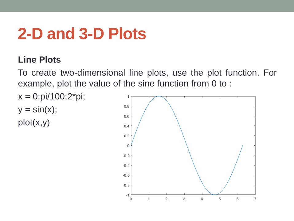
Line Plots
To create two-dimensional line plots, use the plot function. For
example, plot the value of the sine function from 0 to :
x = 0:pi/100:2*pi;
y = sin(x);
plot(x,y)

2-D and 3-D Plots
Line Plots
You can label the axes and add a title.
xlabel('x')
ylabel('sin(x)')
title('Plot of the Sine Function')
2-D and 3-D Plots
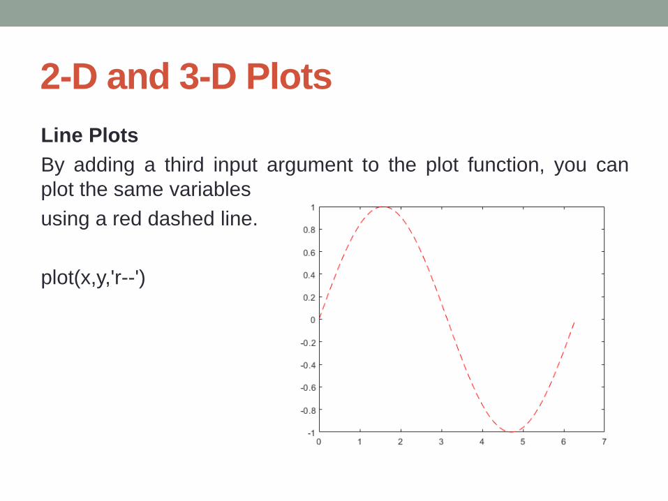
Line Plots
By adding a third input argument to the plot function, you can
plot the same variables
using a red dashed line.
plot(x,y,'r--')

2-D and 3-D Plots
Line Plots
'r--' is a line specification. Each specification can include
characters for the line color, style, and marker. A marker is a
symbol that appears at each plotted data point, such as a
+, o, or *. For example, 'g:*' requests a dotted green line with *
markers.
Notice that the titles and labels that you defined for the first plot
are no longer in the current figure window. By default, MATLAB®
clears the figure each time you call a plotting function, resetting
the axes and other elements to prepare the new plot.

2-D and 3-D Plots
Line Plots
To add plots to an existing figure, use hold on. Until you use hold
off or close the window, all plots appear in the current figure
window.
x = 0:pi/100:2*pi;
y = sin(x);
plot(x,y)
hold on
y2 = cos(x);
plot(x,y2,':')
legend('sin','cos')
hold off

2-D and 3-D Plots
3-D Plots
Three-dimensional plots typically display a surface defined by a
function in two variables,
To evaluate z, first create a set of (x,y) points over the domain of
the function using meshgrid.
[X,Y] = meshgrid(-2:.2:2);
Z = X .* exp(-X.^2 - Y.^2);
Then, create a surface plot.
surf(X,Y,Z)

2-D and 3-D Plots
3-D Plots
Both the surf function
and its companion mesh
display surfaces in three
dimensions. surf displays
both the connecting lines
and the faces of the
surface in color. Mesh
produces wireframe
surfaces that color only
the lines connecting the
defining points.
2-D and 3-D Plots
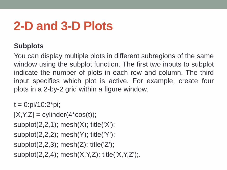
Subplots
You can display multiple plots in different subregions of the same
window using the subplot function. The first two inputs to subplot
indicate the number of plots in each row and column. The third
input specifies which plot is active. For example, create four
plots in a 2-by-2 grid within a figure window.
t = 0:pi/10:2*pi;
[X,Y,Z] = cylinder(4*cos(t));
subplot(2,2,1); mesh(X); title('X');
subplot(2,2,2); mesh(Y); title('Y');
subplot(2,2,3); mesh(Z); title('Z');
subplot(2,2,4); mesh(X,Y,Z); title('X,Y,Z');.

2-D and 3-D Plots
Subplots

Programming and Scripts
Sample Script
To create a script, use the edit command, edit plotrand
This opens a blank file named plotrand.m. Enter some code that
plots a vector of
random data:
n = 50;
r = rand(n,1);
plot(r)

Programming and Scripts
Sample Script
Next, add code that draws a horizontal line on the plot at the
mean:
m = mean(r);
hold on
plot([0,n],[m,m])
hold off
title('Mean of Random Uniform Data')

Programming and Scripts
Sample Script
Whenever you write code, it is a good practice to add comments
that describe the code.
Comments allow others to understand your code, and can
refresh your memory when you return to it later. Add comments
using the percent (%) symbol.
% Generate random data from a uniform distribution
% and calculate the mean. Plot the data and the mean.
n = 50; % 50 data points
r= rand(n,1);
plot(r)

Programming and Scripts
Sample Script
% Draw a line from (0,m) to (n,m)
m = mean(r);
hold on
plot([0,n],[m,m])
hold off
title('Mean of Random Uniform Data')
Save the file in the current folder. To run the script, type its name
at the command line:
plotrand
You can also run scripts from the Editor by pressing the Run
button ….

Loops and Conditional Statements
Within a script, you can loop over sections of code and
conditionally execute sections using the keywords for, while, if,
and switch. For example, create a script named calcmean.m that
uses a for loop to calculate the mean of five random samples
and the overall mean.
nsamples = 5;
npoints = 50;
for k = 1:nsamples
currentData = rand(npoints,1);
sampleMean(k) = mean(currentData);
end
overallMean = mean(sampleMean)

Loops and Conditional Statements
Now, modify the for loop so that you can view the results at each
iteration. Display text in the Command Window that includes the
current iteration number, and remove the semicolon from the
assignment to sampleMean.
for k = 1:nsamples
iterationString = ['Iteration #',int2str(k)];
disp(iterationString)
currentData = rand(npoints,1);
sampleMean(k) = mean(currentData)
end
overallMean = mean(sampleMean)

Loops and Conditional Statements
When you run the script, it displays the intermediate results, and
then calculates the overall mean.
calcmean
Iteration #1
sampleMean =
0.3988
Iteration #2
sampleMean =
0.3988 0.4950

Loops and Conditional Statements
IIteration #3
sampleMean =
0.3988 0.4950 0.5365
teration #4
sampleMean =
0.3988 0.4950 0.5365 0.4870
Iteration #5
sampleMean =
0.3988 0.4950 0.5365 0.4870 0.5501
overallMean =
0.4935

Loops and Conditional Statements
In the Editor, add conditional statements to the end of
calcmean.m that display a different message depending on the
value of overallMean.
if overallMean < .49
disp('Mean is less than expected')
elseif overallMean > .51
disp('Mean is greater than expected')
else
disp('Mean is within the expected range')
end

Loops and Conditional Statements
Run calcmean and verify that the correct message displays for
the calculated overallMean.
For example:
overallMean =
0.5178
Mean is greater than expected.

Loops and Conditional Statements
Script Locations
MATLAB looks for scripts and other files in certain places. To run
a script, the file must be in the current folder or in a folder on the
search path.
By default, the MATLAB folder that the MATLAB Installer creates
is on the search path. If you want to store and run programs in
another folder, add it to the search path.
Select the folder in the Current Folder browser, right-click, and
then select Add to Path.

Help and Documentation
All MATLAB functions have supporting documentation that
includes examples and describes the function inputs, outputs,
and calling syntax.
There are several ways to access this information from the
command line:
• Open the function documentation in a separate window using
the doc command.
doc mean
• Display function hints (the syntax portion of the function
documentation) in the Command Window by pausing after you
type the open parentheses for the function input arguments..

Help and Documentation
mean(
• View an abbreviated text version of the function documentation
in the Command
Window using the help command.
help mean
Access the complete product documentation by clicking the help
icon .
Matrices and Magic Squares
In the MATLAB environment, a matrix is a rectangular array of
numbers.
Special meaning is sometimes attached to 1-by-1 matrices,
which are scalars, and to matrices with only one row or column,
which are vectors.
MATLAB has other ways of storing both numeric and
nonnumeric data, but in the beginning, it is usually best to think
of everything as a matrix.
The operations in MATLAB are designed to be as natural as
possible.
Where other programming languages work with numbers one
at a time, MATLAB allows you to work with entire matrices
quickly and easily.
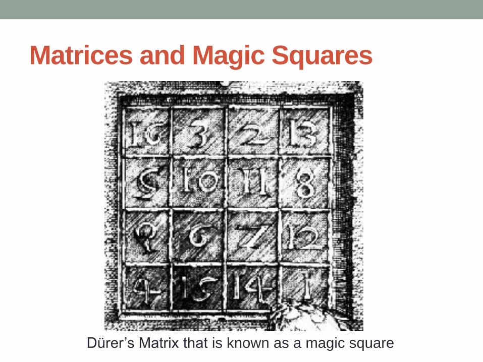
Matrices and Magic Squares
Dürer’s Matrix that is known as a magic square

Matrices and Magic Squares
Entering Matrices
You can enter matrices into MATLAB in several different ways:
• Enter an explicit list of elements.
• Load matrices from external data files.
• Generate matrices using built-in functions.
• Create matrices with your own functions and save them in files.

Matrices and Magic Squares
Entering Matrices
Start by entering Dürer's matrix as a list of its elements. You only
have to follow a few basic conventions:
• Separate the elements of a row with blanks or commas.
• Use a semicolon, ; , to indicate the end of each row.
• Surround the entire list of elements with square brackets, [ ].
To enter Dürer's matrix, simply type in the Command Window
A = [16 3 2 13; 5 10 11 8; 9 6 7 12; 4 15 14 1]

Matrices and Magic Squares
Entering Matrices
MATLAB displays the matrix you just entered:
A =
16 3 2 13
5 10 11 8
9 6 7 12
4 15 14 1
This matrix matches the numbers in the engraving. Once you
have entered the matrix, it is automatically remembered in the
MATLAB workspace. You can refer to it simply as A.
Now that you have A in the workspace, take a look at what
makes it so interesting. Why is it magic?

Matrices and Magic Squares
sum, transpose, and diag
You are probably already aware that the special properties of a
magic square have to do with the various ways of summing its
elements. If you take the sum along any row or column, or along
either of the two main diagonals, you will always get the same
number.
Let us verify that using MATLAB. The first statement to try is
sum(A)
MATLAB replies with
ans =
34 34 34 34

Matrices and Magic Squares
sum, transpose, and diag
When you do not specify an output variable, MATLAB uses the
variable ans, short for answer, to store the results of a
calculation. You have computed a row vector containing the
sums of the columns of A. Each of the columns has the same
sum, the magic sum, 34.
How about the row sums? MATLAB has a preference for
working with the columns of a matrix, so one way to get the row
sums is to transpose the matrix, compute the column sums of
the transpose, and then transpose the result.

Matrices and Magic Squares
sum, transpose, and diag
MATLAB has two transpose operators. The apostrophe
operator (for example, A') performs a complex conjugate
transposition.
It flips a matrix about its main diagonal, and also changes the
sign of the imaginary component of any complex elements of
the matrix.
The dot-apostrophe operator (A.'), transposes without affecting
the sign of complex elements.
For matrices containing all real elements, the two operators
return the same result.

Matrices and Magic Squares
sum, transpose, and diag
A’ produces
ans =
16 5 9 4
3 10 6 15
2 11 7 14
13 8 12 1

Matrices and Magic Squares
sum, transpose, and diag
sum(A')'
produces a column vector containing the row sums
ans =
34
34
34
34

Matrices and Magic Squares
sum, transpose, and diag
For an additional way to sum the rows that avoids the double
transpose use the dimension argument for the sum function:
sum(A,2)
produces
ans =
34
34
34
34

Matrices and Magic Squares
sum, transpose, and diag
The sum of the elements on the main diagonal is obtained with
the sum and the diag functions:
diag(A)
produces
ans =
16
10
7
1

Matrices and Magic Squares
sum, transpose, and diag
sum(diag(A))
produces
ans =
34
The other diagonal, the so-called antidiagonal, is not so
important mathematically, so MATLAB does not have a ready-
made function for it. But a function originally intended for use in
graphics, fliplr, flips a matrix from left to right:
sum(diag(fliplr(A)))
ans =
34

Matrices and Magic Squares
The magic Function
MATLAB actually has a built-in function that creates magic
squares of almost any size.
Not surprisingly, this function is named magic:
B = magic(4)
B =
16 2 3 13
5 11 10 8
9 7 6 12
4 14 15 1

Matrices and Magic Squares
The magic Function
This matrix is almost the same as the one in the Dürer engraving
and has all the same “magic” properties; the only difference is
that the two middle columns are exchanged.
You can swap the two middle columns of B to look like Dürer's A.
For each row of B, rearrange the columns in the order specified
by 1, 3, 2, 4:
A = B(:,[1 3 2 4])
A =
16 3 2 13
5 10 11 8
9 6 7 12
4 15 14 1

Matrices and Magic Squares
Generating Matrices
MATLAB software provides four functions that generate basic
matrices.
zeros All zeros
ones All ones
rand Uniformly distributed random elements
randn Normally distributed random elements
Here are some examples:
Z = zeros(2,4)
Z =
0 0 0 0
0 0 0 0

Matrices and Magic Squares
Generating Matrices
F = 5*ones(3,3)
F =
5 5 5
5 5 5
5 5 5
N = fix(10*rand(1,10))
N =
9 2 6 4 8 7 4 0 8 4

Matrices and Magic Squares
Generating Matrices
R = randn(4,4)
R =
0.6353 0.0860 -0.3210 -1.2316
-0.6014 -2.0046 1.2366 1.0556
0.5512 -0.4931 -0.6313 -0.1132
-1.0998 0.4620 -2.3252 0.3792

Expressions
Variables
The MATLAB language provides mathematical expressions, but
unlike most programming languages, these expressions involve
entire matrices.
MATLAB does not require any type declarations or dimension
statements. When MATLAB encounters a new variable name, it
automatically creates the variable and allocates the appropriate
amount of storage. If the variable already exists, MATLAB
changes its contents and, if necessary, allocates new storage.
num_students = 25
creates a 1-by-1 matrix named num_students and stores the
value 25 in its single element. To view the matrix assigned to any
variable, simply enter the variable name.

Expressions
Variables
Variable names consist of a letter, followed by any number of
letters, digits, or underscores. MATLAB is case sensitive; it
distinguishes between uppercase and lowercase letters. A and a
are not the same variable.
Although variable names can be of any length, MATLAB uses
only the first N characters of the name, (where N is the number
returned by the function namelengthmax), and ignores the rest.
Hence, it is important to make each variable name unique in the
first N characters to enable MATLAB to distinguish variables.
N = namelengthmax
N =
63
Expressions
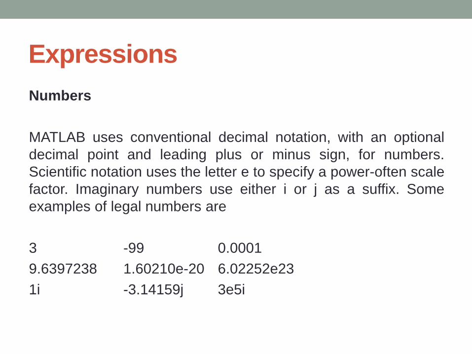
Numbers
MATLAB uses conventional decimal notation, with an optional
decimal point and leading plus or minus sign, for numbers.
Scientific notation uses the letter e to specify a power-often scale
factor. Imaginary numbers use either i or j as a suffix. Some
examples of legal numbers are
3 -99 0.0001
9.6397238 1.60210e-20 6.02252e23
1i -3.14159j 3e5i

Expressions
Numbers
MATLAB stores all numbers internally using the long format
specified by the IEEE® floating-point standard. Floating-point
numbers have a finite precision of roughly 16 significant decimal
digits and a finite range of roughly 10-308 to 10+308.
Numbers represented in the double format have a maximum
precision of 52 bits. Any double requiring more bits than 52 loses
some precision. For example, the following code shows two
unequal values to be equal because they are both truncated:
x = 36028797018963968; y = 36028797018963972;
x == y
ans =
1

Expressions
Numbers
Integers have available precisions of 8-bit, 16-bit, 32-bit, and 64-
bit. Storing the same numbers as 64-bit integers preserves
precision:
x = uint64(36028797018963968);
y = uint64(36028797018963972);
x == y
ans = 0
MATLAB software stores the real and imaginary parts of a
complex number. It handles the magnitude of the parts in
different ways depending on the context. For instance, the sort
function sorts based on magnitude and resolves ties by phase
angle.
Expressions
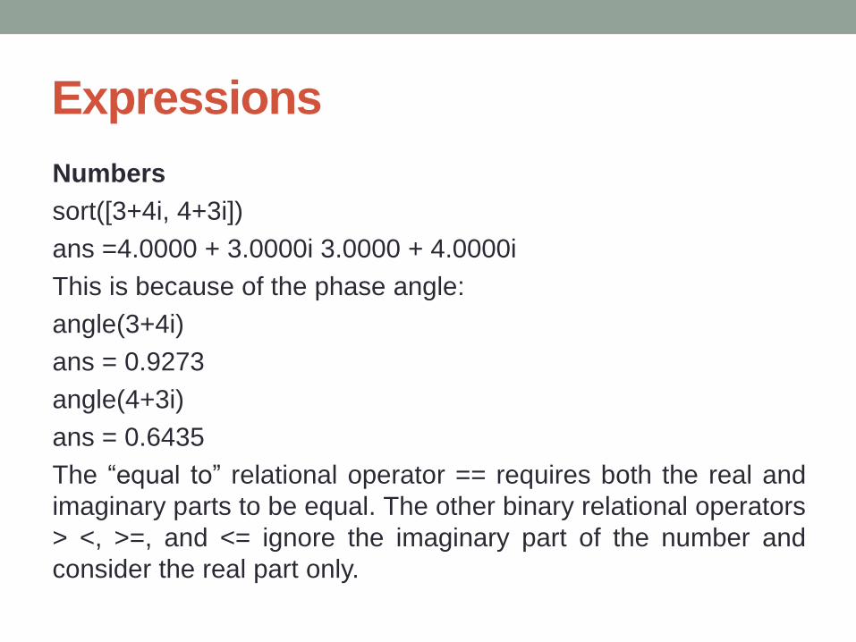
Numbers
sort([3+4i, 4+3i])
ans =4.0000 + 3.0000i 3.0000 + 4.0000i
This is because of the phase angle:
angle(3+4i)
ans = 0.9273
angle(4+3i)
ans = 0.6435
The “equal to” relational operator == requires both the real and
imaginary parts to be equal. The other binary relational operators
> <, >=, and <= ignore the imaginary part of the number and
consider the real part only.

Expressions
Matrix Operators
Expressions use familiar arithmetic operators and precedence
rules.
+ Addition
- Subtraction
* Multiplication
/ Division
\ Left division
^ Power
' Complex conjugate transpose
( ) Specify evaluation order.

Expressions
Array Operators
When they are taken away from the world of linear algebra,
matrices become two-dimensional numeric arrays.
Arithmetic operations on arrays are done element by element.
This means that addition and subtraction are the same for
arrays and matrices, but that multiplicative operations are
different.
MATLAB uses a dot, or decimal point, as part of the notation
for multiplicative array operations.

Expressions
Array Operators
The list of operators includes
+ Addition
- Subtraction
.* Element
./ Element-by-element division
.\ Element-by-element left division
.^ Element-by-element power
.' Unconjugated array transpose

MATLAB Tutorial
Part 2

CONTENTS
Quick Start
Language Fundamentals
Mathematics
Graphics
Programming

Expressions
Array Operators
The list of operators includes
+ Addition
- Subtraction
.* Element
./ Element-by-element division
.\ Element-by-element left division
.^ Element-by-element power
.' Unconjugated array transpose
Expressions
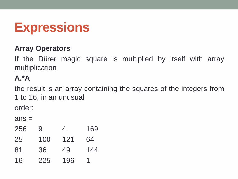
Array Operators
If the Dürer magic square is multiplied by itself with array
multiplication
A.*A
the result is an array containing the squares of the integers from
1 to 16, in an unusual
order:
ans =
256 9 4 169
25 100 121 64
81 36 49 144
16 225 196 1

Expressions
Building Tables
Array operations are useful for building tables. Suppose n is the
column vector
n = (0:9)';
Then
pows = [n n.^2 2.^n]
builds a table of squares and powers of 2: pows = 0 0 1
1 1 2
2 4 4
3 9 8
4 16 16
5 25 32
6 36 64
7 49 128
8 64 256
9 81 512

Expressions
Building Tables
The elementary math functions operate on arrays element by
element.
So
format short g
x = (1:0.1:2)';
logs = [x log10(x)]
builds a table of logarithms.

Expressions
Building Tables
logs =
1.0 0
1.1 0.04139
1.2 0.07918
1.3 0.11394
1.4 0.14613
1.5 0.17609
1.6 0.20412
1.7 0.23045
1.8 0.25527
1.9 0.27875
2.0 0.30103.

Expressions
Functions
MATLAB provides a large number of standard elementary
mathematical functions, including abs, sqrt, exp, and sin.
Taking the square root or logarithm of a negative number is not
an error; the appropriate complex result is produced
automatically.
MATLAB also provides many more advanced mathematical
functions, including Bessel and gamma functions. Most of
these functions accept complex arguments. For a list of the
elementary mathematical functions, type
help elfun

Expressions
Functions
For a list of more advanced mathematical and matrix functions,
type
help specfun
help elmat
Some of the functions, like sqrt and sin are built in. Built-in
functions are part of the MATLAB core so they are very efficient,
but the computational details are not readily accessible. Other
functions are implemented in the MATLAB programing language,
so their computational details are accessible. There are some
differences between built-in functions and other functions. For
example, for built-in functions, you cannot see the code. For
other functions, you can see the code and even modify it if you
want.

Expressions
Functions
Several special functions provide values of useful constants.
pi 3.14159265...
i Imaginary unit, −1
j Same as i
Eps Floating-point relative precision, =2-52
realmin Smallest floating-point number, 2-1022
realmax Largest floating-point number, (2- )21023
Inf Infinity
NaN Not-a-number

Expressions
Functions
Infinity is generated by dividing a nonzero value by zero, or by
evaluating well defined mathematical expressions that overflow,
that is, exceed realmax. Not-a-number is generated by trying to
evaluate expressions like 0/0 or Inf-Inf that do not have well
defined mathematical values.
The function names are not reserved. It is possible to overwrite
any of them with a new variable, such as
eps = 1.e-6
and then use that value in subsequent calculations. The original
function can be restored
with
clear eps

Expressions
Examples of Expressions
You have already seen several examples of MATLAB
expressions. Here are a few more examples, and the resulting
values:
rho = (1+sqrt(5))/2
rho =
1.6180
a = abs(3+4i)
a =
5

Expressions
Examples of Expressions
z = sqrt(besselk(4/3,rho-i))
z =
0.3730+ 0.3214i
huge = exp(log(realmax))
huge =
1.7977e+308
toobig = pi*huge
toobig =
Inf

Entering Commands
The format Function
The format function controls the numeric format of the values
displayed.
The function affects only how numbers are displayed, not how
MATLAB software computes or saves them.
Here are the different formats, together with the resulting
output produced from a vector x with components of different
magnitudes.

Entering Commands
The format Function
x = [4/3 1.2345e-6]
format short
1.3333 0.0000
format short e
1.3333e+000 1.2345e-006
format short g
1.3333 1.2345e-006
format long
1.33333333333333 0.00000123450000
format long e
1.333333333333333e+000 1.234500000000000e-006

Entering Commands
The format Function
format long g
1.33333333333333 1.2345e-006
format bank
1.33 0.00
format rat
4/3 1/810045
format hex
3ff5555555555555 3eb4b6231abfd271

Entering Commands
The format Function
If the largest element of a matrix is larger than 103 or smaller
than 10-3, MATLAB applies a common scale factor for the
short and long formats.
In addition to the format functions shown above format
compact suppresses many of the blank lines that appear in the
output.
This lets you view more information on a screen or window. If
you want more control over the output format, use the sprintf
and fprintf functions.

Entering Commands
Suppressing Output
If you simply type a statement and press Return or Enter,
MATLAB automatically displays the results on screen.
However, if you end the line with a semicolon, MATLAB performs
the computation, but does not display any output.
This is particularly useful when you generate large matrices. For
example,
A = magic(100);.

Entering Commands
Entering Long Statements
If a statement does not fit on one line, use an ellipsis (three
periods), ..., followed by
Return or Enter to indicate that the statement continues on the
next line. For example,
s = 1 -1/2 + 1/3 -1/4 + 1/5 - 1/6 + 1/7 ...
- 1/8 + 1/9 - 1/10 + 1/11 - 1/12;
Blank spaces around the =, +, and - signs are optional, but they
improve readability.

Entering Commands
Command Line Editing
Various arrow and control keys on your keyboard allow you to
recall, edit, and reuse statements you have typed earlier. For
example, suppose you mistakenly enter
rho = (1 + sqt(5))/2
You have misspelled sqrt. MATLAB responds with
Undefined function 'sqt' for input arguments of type 'double'.
Instead of retyping the entire line, simply press the ↑ key. The
statement you typed is redisplayed. Use the ← key to move the
cursor over and insert the missing r. Repeated use of the ↑ key
recalls earlier lines. Typing a few characters, and then pressing
the ↑ key finds a previous line that begins with those characters.
You can also copy previously executed statements from the
Command History.

Indexing
Subscripts
The element in row i and column j of A is denoted by A(i,j). For
example, A(4,2) is the number in the fourth row and second
column. For the magic square, A(4,2) is 15. So to compute the
sum of the elements in the fourth column of A, type
A(1,4) + A(2,4) + A(3,4) + A(4,4)
This subscript produces
ans =
34
but is not the most elegant way of summing a single column.
Indexing
Subscripts
It is also possible to refer to the elements of a matrix with a
single subscript, A(k). A single subscript is the usual way of
referencing row and column vectors. However, it can also apply
to a fully two-dimensional matrix, in which case the array is
regarded as one long column vector formed from the columns of
the original matrix. So, for the magic square, A(8) is another way
of referring to the value 15 stored in A(4,2).
If you try to use the value of an element outside of the matrix, it
is an error:
t = A(4,5)
Index exceeds matrix dimensions.

Indexing
Subscripts
Conversely, if you store a value in an element outside of the
matrix, the size increases to accommodate the newcomer:
X = A;
X(4,5) = 17
X =
16 3 2 13 0
5 10 11 8 0
9 6 7 12 0
4 15 14 1 17
Indexing
The Colon Operator
The colon, :, is one of the most important MATLAB operators. It
occurs in several different forms. The expression
1:10
is a row vector containing the integers from 1 to 10:
1 2 3 4 5 6 7 8 9 10
To obtain nonunit spacing, specify an increment. For example,
100:-7:50
is
100 93 86 79 72 65 58 51

Indexing
The Colon Operator
0:pi/4:pi
is
0 0.7854 1.5708 2.3562 3.1416
Subscript expressions involving colons refer to portions of a
matrix:
A(1:k,j)
is the first k elements of the jth column of A. Thus, sum(A(1:4,4))
computes the sum of the fourth column. However, there is a
better way to perform this computation. The colon by itself refers
to all the elements in a row or column of a matrix and the
keyword end refers to the last row or column.

Indexing
The Colon Operator
sum(A(:,end))
computes the sum of the elements in the last column of A:
ans =
34
Why is the magic sum for a 4-by-4 square equal to 34? If the
integers from 1 to 16 are
sorted into four groups with equal sums, that sum must be
sum(1:16)/4
which, of course, is
ans =
34

Indexing
Concatenation
Concatenation is the process of joining small matrices to make
bigger ones. In fact, you made your first matrix by
concatenating its individual elements.
The pair of square brackets, [ ], is the concatenation operator.
For an example, start with the 4-by-4 magic square, A, and
form
B = [A A+32; A+48 A+16]

Indexing
Concatenation
The result is an 8-by-8 matrix, obtained by joining the four
submatrices:
B =
16 3 2 13 48 35 34 45
5 10 11 8 37 42 43 40
9 6 7 12 41 38 39 44
4 15 14 1 36 47 46 33
64 51 50 61 32 19 18 29
53 58 59 56 21 26 27 24
57 54 55 60 25 22 23 28
52 63 62 49 20 31 30 17

Indexing
Concatenation
This matrix is halfway to being another magic square. Its
elements are a rearrangement of the integers 1:64. Its column
sums are the correct value for an 8-by-8 magic square:
sum(B)
ans =
260 260 260 260 260 260 260 260
But its row sums, sum(B')', are not all the same. Further
manipulation is necessary to make this a valid 8-by-8 magic
square.

Indexing
Deleting Rows and Columns
You can delete rows and columns from a matrix using just a pair
of square brackets. Start with
X = A;
Then, to delete the second column of X, use
X(:,2) = [ ]
This changes X to
X =
16 2 13
5 11 8
9 7 12
4 14 1

Indexing
Deleting Rows and Columns
If you delete a single element from a matrix, the result is not a
matrix anymore. So, expressions like
X(1,2) = [ ]
result in an error. However, using a single subscript deletes a
single element, or sequence
of elements, and reshapes the remaining elements into a row
vector. So
X(2:2:10) = [ ]
results in
X =
16 9 2 7 13 12 1

Indexing
Scalar Expansion
Matrices and scalars can be combined in several different ways.
For example, a scalar is subtracted from a matrix by subtracting
it from each element. The average value of the elements in our
magic square is 8.5, so
B = A - 8.5
forms a matrix whose column sums are zero:
B =
7.5 -5.5 -6.5 4.5
-3.5 1.5 2.5 -0.5
0.5 -2.5 -1.5 3.5
-4.5 6.5 5.5 -7.5

Indexing
Scalar Expansion
sum(B)
ans = 0 0 0 0
With scalar expansion, MATLAB assigns a specified scalar to all
indices in a range. Forexample,
B(1:2,2:3) = 0
zeros out a portion of B:
B =
7.5 0 0 4.5
-3.5 0 0 -0.5
0.5 -2.5 -1.5 3.5
-4.5 6.5 5.5 -7.5

Indexing
Logical Subscripting
The logical vectors created from logical and relational operations
can be used to reference subarrays. Suppose X is an ordinary
matrix and L is a matrix of the same size that is the result of
some logical operation. Then X(L) specifies the elements of X
where the elements of L are nonzero.
This kind of subscripting can be done in one step by specifying
the logical operation as the subscripting expression.
Suppose you have the following set of data:
x = [2.1 1.7 1.6 1.5 NaN 1.9 1.8 1.5 5.1 1.8 1.4 2.2 1.6 1.8];

Indexing
Logical Subscripting
The NaN is a marker for a missing observation, such as a failure
to respond to an item on a questionnaire. To remove the missing
data with logical indexing, use isfinite(x), which is true for all
finite numerical values and false for NaN and Inf:
x = x(isfinite(x))
x =
2.1 1.7 1.6 1.5 1.9 1.8 1.5 5.1 1.8 1.4 2.2 1.6 1.8

Indexing
Logical Subscripting
Now there is one observation, 5.1, which seems to be very
different from the others. It is an outlier.
The following statement removes outliers, in this case those
elements more than three standard deviations from the mean:
x = x(abs(x-mean(x)) <= 3*std(x))
x =
2.1 1.7 1.6 1.5 1.9 1.8 1.5 1.8 1.4 2.2 1.6 1.8
Indexing
Logical Subscripting
For another example, highlight the location of the prime numbers
in Dürer's magic square by using logical indexing and scalar
expansion to set the nonprimes to 0. (See .)
A(~isprime(A)) = 0
A =
0 3 2 13
5 0 11 0
0 0 7 0
0 0 0 0

Indexing
The find Function
The find function determines the indices of array elements that
meet a given logical condition. In its simplest form, find returns a
column vector of indices. Transpose that vector to obtain a row
vector of indices. For example, start again with Dürer's magic
square. (See .)
k = find(isprime(A))'
picks out the locations, using one-dimensional indexing, of the
primes in the magic square:
k =
2 5 9 10 11 13

Indexing
The find Function
Display those primes, as a row vector in the order determined by
k, with A(k)
ans = 5 3 2 11 7 13
When you use k as a left-side index in an assignment statement,
the matrix structure is preserved:
A(k) = NaN
A =
16 NaN NaN NaN
NaN 10 NaN 8
9 6 NaN 12
4 15 14 1

Types of Arrays
Multidimensional Arrays
Multidimensional arrays in the MATLAB environment are arrays
with more than two subscripts. One way of creating a
multidimensional array is by calling zeros, ones, rand, or randn
with more than two arguments. For example,
R = randn(3,4,5);
creates a 3-by-4-by-5 array with a total of 3*4*5 = 60 normally
distributed random elements.

Types of Arrays
Multidimensional Arrays
A three-dimensional array might represent three-dimensional
physical data, say the temperature in a room, sampled on a
rectangular grid. Or it might represent a sequence of matrices,
A(k), or samples of a time-dependent matrix, A(t). In these latter
cases, the (i, j)th element of the kth matrix, or the tkth matrix, is
denoted by A(i,j,k).
MATLAB and Dürer's versions of the magic square of order 4
differ by an interchange of two columns. Many different magic
squares can be generated by interchanging columns.

Types of Arrays
Multidimensional Arrays
The statement
p = perms(1:4);
generates the 4! = 24 permutations of 1:4. The kth permutation is
the row vector
p(k,:). Then
A = magic(4);
M = zeros(4,4,24);
for k = 1:24
M(:,:,k) = A(:,p(k,:));
end

Types of Arrays
Multidimensional Arrays
stores the sequence of 24 magic squares in a three-dimensional
array, M. The size of M is
size(M)
ans =
4 4 24

Types of Arrays
Multidimensional Arrays
The statement
sum(M,d)
computes sums by varying the dth subscript. So
sum(M,1)
is a 1-by-4-by-24 array containing 24 copies of the row vector
34 34 34 34
and
Note: The order of the matrices shown in this illustration might differ from your
results. The perms function always returns all permutations of the input vector,
but the order of the permutations might be different for different MATLAB
versions.

Types of Arrays
Multidimensional Arrays
sum(M,2)
is a 4-by-1-by-24 array containing 24 copies of the column vector
34
34
34
34

Types of Arrays
Multidimensional Arrays
Finally,
S = sum(M,3)
adds the 24 matrices in the sequence. The result has size 4-by-
4-by-1, so it looks like a 4by-4 array:
S =
204 204 204 204
204 204 204 204
204 204 204 204
204 204 204 204

Types of Arrays
Cell Arrays
Cell arrays in MATLAB are multidimensional arrays whose
elements are copies of other arrays. A cell array of empty
matrices can be created with the cell function. But, more often,
cell arrays are created by enclosing a miscellaneous collection of
things in curly braces, { }.
The curly braces are also used with subscripts to access the
contents of various cells. For example,
C = {A sum(A) prod(prod(A))}
produces a 1-by-3 cell array. The three cells contain the magic
square, the row vector of column sums, and the product of all its
elements.

Types of Arrays
Cell Arrays
C =
[4x4 double] [1x4 double] [20922789888000]
This is because the first two cells are too large to print in this
limited space, but the third cell contains only a single number,
16!, so there is room to print it.
Here are two important points to remember. First, to retrieve the
contents of one of the cells, use subscripts in curly braces. For
example, C{1} retrieves the magic square and C{3} is 16!.
Second, cell arrays contain copies of other arrays, not pointers
to those arrays. If you subsequently change A, nothing happens
to C.

Types of Arrays
Cell Arrays
You can use three-dimensional arrays to store a sequence of
matrices of the same size.
Cell arrays can be used to store a sequence of matrices of
different sizes. For example,
M = cell(8,1);
for n = 1:8
M{n} = magic(n);
end
M
produces a sequence of magic squares of different order:
Types of Arrays
Cell Arrays
M =
[ 1]
[ 2x2 double]
[ 3x3 double]
[ 4x4 double]
[ 5x5 double]
[ 6x6 double]
[ 7x7 double]
[ 8x8 double]

Types of Arrays
Cell Arrays
You can retrieve
the 4-by-4 magic square
matrix with
M{4}

Types of Arrays
Characters and Text
Enter text into MATLAB using single quotes. For example,
s = 'Hello'
The result is not the same kind of numeric matrix or array you
have been dealing with up to now. It is a 1-by-5 character array.
statement
a = double(s)
converts the character array to a numeric matrix containing
floating-point representations of the ASCII codes for each
character. The result is
a =
72 101 108 108 111

Types of Arrays
Characters and Text
The statement
s = char(a)
reverses the conversion.
Converting numbers to characters makes it possible to
investigate the various fonts available on your computer. The
printable characters in the basic ASCII character set are
represented by the integers 32:127. (The integers less than 32
represent nonprintable control characters.) These integers are
arranged in an appropriate 6-by-16 array with
F = reshape(32:127,16,6)';

Types of Arrays
Characters and Text
The printable characters in the extended ASCII character set are
represented by F+128.
When these integers are interpreted as characters, the result
depends on the font currently being used. Type the statements
char(F)
char(F+128)
and then vary the font being used for the Command Window. To
change the font, on the Home tab, in the Environment section,
click Preferences > Fonts. If you include tabs in lines of code,
use a fixed-width font, such as Monospaced, to align the tab
positions on different lines.
Types of Arrays
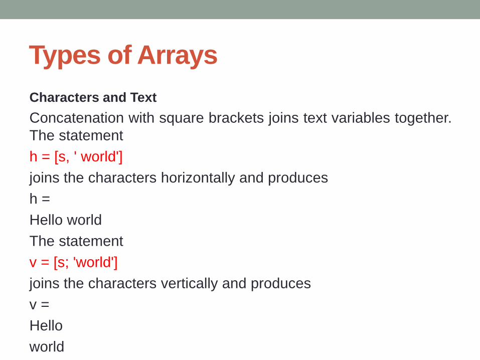
Characters and Text
Concatenation with square brackets joins text variables together.
The statement
h = [s, ' world']
joins the characters horizontally and produces
h =
Hello world
The statement
v = [s; 'world']
joins the characters vertically and produces
v =
Hello
world

Types of Arrays
Characters and Text
Notice that a blank has to be inserted before the 'w' in h and that
both words in v have to have the same length. The resulting
arrays are both character arrays; h is 1-by-11 and v is 2-by-5.
To manipulate a body of text containing lines of different lengths,
you have two choices—a padded character array or a cell array
of character vectors. When creating a character array, you must
make each row of the array the same length. (Pad the ends of
the shorter rows with spaces.) The char function does this
padding for you.

Types of Arrays
Characters and Text
S = char('A','rolling','stone','gathers','momentum.')
produces a 5-by-9 character array:
S =
A
rolling
stone
gathers
momentum.

Types of Arrays
Characters and Text
Alternatively, you can store the text in a cell array. For example,
C = {'A';'rolling';'stone';'gathers';'momentum.'}
creates a 5-by-1 cell array that requires no padding because
each row of the array can
have a different length:
C =
'A'
'rolling'
'stone'
'gathers'
'momentum.'

Types of Arrays
Characters and Text
You can convert a padded character array to a cell array of
character vectors with
C = cellstr(S)
and reverse the process with
S = char(C)

Types of Arrays
Structures
Structures are multidimensional MATLAB arrays with elements
accessed by textual field designators. For example,
S.name = 'Ed Plum';
S.score = 83;
S.grade = 'B+'
creates a scalar structure with three fields:
S =
name: 'Ed Plum'
score: 83
grade: 'B+'

Types of Arrays
Structures
Like everything else in the MATLAB environment, structures are
arrays, so you can insert additional elements. In this case, each
element of the array is a structure with several fields. The fields
can be added one at a time,
S(2).name = 'Toni Miller';
S(2).score = 91;
S(2).grade = 'A-';
or an entire element can be added with a single statement:
S(3) = struct('name','Jerry Garcia',...
'score',70,'grade','C')

Types of Arrays
Structures
Now the structure is large enough that only a summary is
printed:
S =
1x3 struct array with fields:
name
score
grade
There are several ways to reassemble the various fields into
other MATLAB arrays. They are mostly based on the notation of
a comma-separated list.

Types of Arrays
Structures
If you type
S.score
it is the same as typing S(1).score, S(2).score, S(3).score which
is a comma-separated list.
If you enclose the expression that generates such a list within
square brackets, MATLAB stores each item from the list in an
array. In this example, MATLAB creates a numeric row vector
containing the score field of each element of structure array S:

Types of Arrays
Structures
scores = [S.score]
scores =
83 91 70
avg_score = sum(scores)/length(scores)
avg_score =
81.3333

Types of Arrays
Structures
To create a character array from one of the text fields (name, for
example), call the char function on the comma-separated list
produced by S.name:
names = char(S.name)
names =
Ed Plum
Toni Miller
Jerry Garcia
Similarly, you can create a cell

Types of Arrays
Structures
Similarly, you can create a cell array from the name fields by
enclosing the list-generating expression within curly braces:
names = {S.name}
names =
'Ed Plum' 'Toni Miller' 'Jerry Garcia'
To assign the fields of each element of a structure array to
separate variables outside of the structure, specify each output
to the left of the equals sign, enclosing them all within square
brackets:

Types of Arrays
Structures
[N1 N2 N3] = S.name
N1 =
Ed Plum
N2 =
Toni Miller
N3 =
Jerry Garcia

Types of Arrays
Dynamic Field Names
The most common way to access the data in a structure is by
specifying the name of the field that you want to reference.
Another means of accessing structure data is to use dynamic
field names.
These names express the field as a variable expression that
MATLAB evaluates at run time. The dot-parentheses syntax
shown here makes expression a dynamic field name:
structName.(expression)

Types of Arrays
Dynamic Field Names
Index into this field using the standard MATLAB indexing syntax.
For example, to evaluate expression into a field name and obtain
the values of that field at columns 1 through 25 of row 7, use
structName.(expression)(7,1:25)

Types of Arrays
Dynamic Field Names Example
The avgscore function shown below computes an average test
score, retrieving information from the testscores structure using
dynamic field names:
function avg = avgscore(testscores, student, first, last)
for k = first:last
scores(k) = testscores.(student).week(k);
end
avg = sum(scores)/(last - first + 1);

Types of Arrays
Dynamic Field Names Example
Now run avgscore, supplying the students name fields for the
testscores structure at run time using dynamic field names:
avgscore(testscores, 'Ann_Lane', 7, 22)
ans =
85.2500
avgscore(testscores, 'William_King', 7, 22)
ans =
87.7500

Types of Arrays
Dynamic Field Names Example
You can run this function using different values for the dynamic
field student. First, initialize the structure that contains scores for
a 25-week period:
testscores.Ann_Lane.week(1:25) = ...
[95 89 76 82 79 92 94 92 89 81 75 93 ...
85 84 83 86 85 90 82 82 84 79 96 88 98];
testscores.William_King.week(1:25) = ... [87 80 91 84 99 87 93
87 97 87 82 89 ...
86 82 90 98 75 79 92 84 90 93 84 78 81];


MATLAB Tutorial
Parts 3 and 4

Mathematics

CONTENTS
Linear Algebra
Operations on Nonlinear Functions
Multivariate Data
Data Analysis

Linear Algebra
This topic contains an introduction to creating matrices and
performing basic matrix calculations in MATLAB.
The MATLAB environment uses the term matrix to indicate a
variable containing real or complex numbers arranged in a two-
dimensional grid.
An array is, more generally, a vector, matrix, or higher
dimensional grid of numbers.
All arrays in MATLAB are rectangular, in the sense that the
component vectors along any dimension are all the same
length.
The mathematical operations defined on matrices are the
subject of linear algebra.
Linear Algebra
Creating Matrices
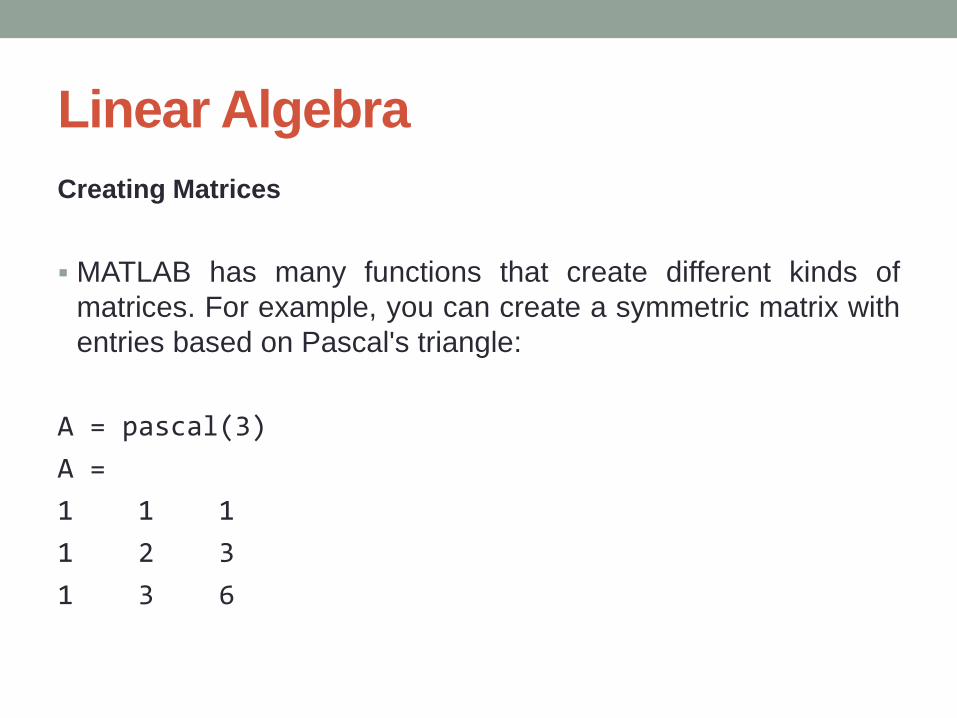
MATLAB has many functions that create different kinds of
matrices. For example, you can create a symmetric matrix with
entries based on Pascal's triangle:
A = pascal(3)
A =
1 1 1
1 2 3
1 3 6

Linear Algebra
Creating Matrices
Or, you can create an unsymmetric magic square matrix, which
has equal row and column sums:
B = magic(3)
B =
8 1 6
3 5 7
4 9 2

Linear Algebra
Creating Matrices
Another example is a 3-by-2 rectangular matrix of random
integers. In this case the first input to randi describes the
range of possible values for the integers, and the second two
inputs describe the number of rows and columns:
C = randi(10,3,2)
C =
9 10
10 7
2 1

Linear Algebra
Creating Matrices
A column vector is an m-by-1 matrix, a row vector is a 1-by-n
matrix, and a scalar is a 1- by-1 matrix.
To define a matrix manually, use square brackets [ ] to denote
the beginning and end of the array.
Within the brackets, use a semicolon ; to denote the end of a
row. In the case of a scalar (1-by-1 matrix), the brackets are not
required.

Linear Algebra
Creating Matrices
For example, these statements produce a column vector, a row
vector, and a scalar.
u = [3; 1; 4]
v = [2 0 -1]
s = 7
u =
3
1
4
v =
2 0 -1
s =
7
Linear Algebra
Adding and Subtracting Matrices
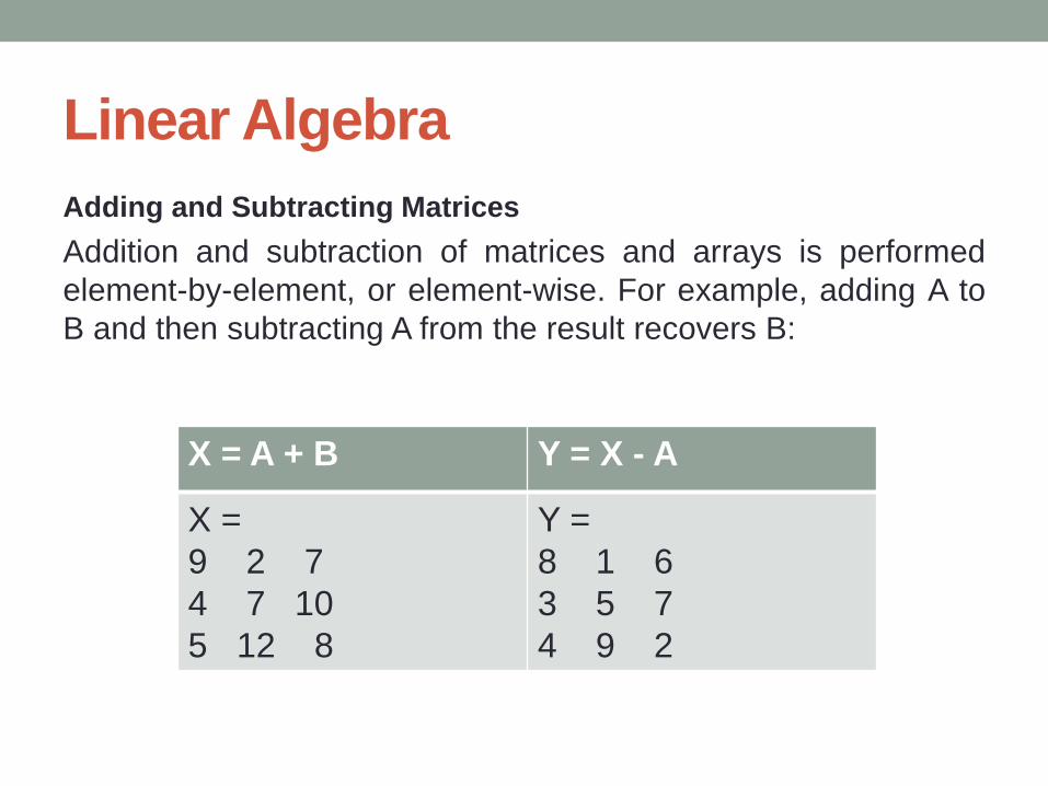
Addition and subtraction of matrices and arrays is performed
element-by-element, or element-wise. For example, adding A to
B and then subtracting A from the result recovers B:
X = A + B Y = X - A
X =
9 2 7
4 7 10
5 12 8
Y =
8 1 6
3 5 7
4 9 2

Linear Algebra
Creating Matrices
Addition and subtraction require both matrices to have
compatible dimensions. If the dimensions are incompatible, an
error results:
X = A + C
Error using +
Matrix dimensions must agree.
For more information, see “Array vs. Matrix Operations”.

Linear Algebra
Vector Products and Transpose
A row vector and a column vector of the same length can be
multiplied in either order. The result is either a scalar, called the
inner product, or a matrix, called the outer product:
Given matrices X = u*v
u = [3; 1; 4]; v = [2 0 -1]; x = v*u x = 2
X = 6 0 -3 2 0 -1 8 0 -4

Linear Algebra
Vector Products and Transpose
For real matrices, the transpose operation interchanges aij and
aji.
For complex matrices, another consideration is whether to take
the complex conjugate of complex entries in the array to form
the complex conjugate transpose.
MATLAB uses the apostrophe operator (') to perform a complex
conjugate transpose, and the dot-apostrophe operator (.') to
transpose without conjugation.
For matrices containing all real elements, the two operators
return the same result.

Linear Algebra
Vector Products and Transpose
The example matrix A = pascal(3) is symmetric, so A' is equal to
A. However, B = magic(3) is not symmetric, so B' has the
elements reflected along the main diagonal:
B = magic(3)
Given matrix X = B'
B = 8 1 6 3 5 7 4 9 2
X = 8 3 4 1 5 9 6 7 2

Linear Algebra
Vector Products and Transpose
For vectors, transposition turns a row vector into a column vector
(and vice-versa):
x = v'
x =
2
0
-1
If x and y are both real column vectors, then the product x*y is
not defined, but the two products x'*y and y'*x produce the same
scalar result. This quantity is used so frequently, it has three
different names: inner product, scalar product, or dot product.
There is even a dedicated function for dot products named dot.

Linear Algebra
Vector Products and Transpose
For a complex vector or matrix, z, the quantity z' not only
transposes the vector or matrix, but also converts each complex
element to its complex conjugate.
That is, the sign of the imaginary part of each complex element
changes. For example, consider the complex matrix.
z = [1+2i 7-3i 3+4i; 6-2i 9i 4+7i]
z = 1.0000 + 2.0000i 7.0000 - 3.0000i 3.0000 + 4.0000i 6.0000 - 2.0000i 0.0000 + 9.0000i 4.0000 + 7.0000i

Linear Algebra
Vector Products and Transpose
The complex conjugate transpose of z is:
z'
ans =
1.0000 - 2.0000i 6.0000 + 2.0000i 7.0000 + 3.0000i 0.0000 - 9.0000i 3.0000 - 4.0000i 4.0000 - 7.0000i

Linear Algebra
Vector Products and Transpose
The unconjugated complex transpose, where the complex part of
each element retains its sign, is denoted by z.' :
For complex vectors, the two scalar products x'*y and y'*x are
complex conjugates of each other, and the scalar product x'*x of
a complex vector with itself is real.
z.'
ans =
1.0000 + 2.0000i 6.0000 - 2.0000i 7.0000 - 3.0000i 0.0000 + 9.0000i 3.0000 + 4.0000i 4.0000 + 7.0000i

Linear Algebra
Multiplying Matrices
Multiplication of matrices is defined in a way that reflects
composition of the underlying linear transformations and allows
compact representation of systems of simultaneous linear
equations.
The matrix product C = AB is defined when the column
dimension of A is equal to the row dimension of B, or when one
of them is a scalar.
If A is m-by-p and B is p-by-n, their product C is m-by-n.

Linear Algebra
Multiplying Matrices
The product can actually be defined using MATLAB for loops,
colon notation, and vector dot products:
A = pascal(3);
B = magic(3);
m = 3;
n = 3;
for i = 1:m
for j = 1:n
C(i,j) = A(i,:)*B(:,j);
end
end

Linear Algebra
Multiplying Matrices
MATLAB uses an asterisk to denote matrix multiplication, as in
C = A*B. Matrix multiplication is not commutative; that is, A*B is
typically not equal to B*A:
X = A*B Y = B*A
X = 15 15 15 26 38 26 41 70 39
Y = 15 28 47 15 34 60 15 28 43

Linear Algebra
Multiplying Matrices
Rectangular matrix multiplications must satisfy the dimension
compatibility conditions.
Since A is 3-by-3 and C is 3-by-2, you can multiply them to get a
3-by-2 result (the common inner dimension cancels). However,
the multiplication does not work in the reverse order:
X = A*C Y = C*A
X = 24 17 47 42 79 77
Error using * Incorrect dimensions for matrix multiplication. Check that the number of columns in the first matrix matches the number of rows in the second matrix. To perform elementwise multiplication, use '.*'.

Linear Algebra
Multiplying Matrices
You can multiply anything with a scalar:
s = 10;
w = s*y
w =
120 -70 100
When you multiply an array by a scalar, the scalar implicitly
expands to be the same size as the other input. This is often
referred to as scalar expansion.

Linear Algebra
Identity Matrix
Generally accepted mathematical notation uses the capital letter
I to denote identity matrices, matrices of various sizes with ones
on the main diagonal and zeros elsewhere. These matrices have
the property that AI = A and IA = A whenever the dimensions are
compatible. The original version of MATLAB could not use I for
this purpose because it did not distinguish between uppercase
and lowercase letters and i already served as a subscript and as
the complex unit. So an English language pun was introduced.
The function
eye(m,n)
returns an m-by-n rectangular identity matrix and eye(n) returns
an n-by-n square identity matrix.

Linear Algebra
Kronecker Tensor Product
The Kronecker product, kron(X,Y), of two matrices is the larger
matrix formed from all possible products of the elements of X
with those of Y. If X is m-by-n and Y is p-by-q, then kron(X,Y) is
mp-by-nq. The elements are arranged such that each element of
X is multiplied by the entire matrix Y:
[X(1,1)*Y X(1,2)*Y . . . X(1,n)*Y
. . .
X(m,1)*Y X(m,2)*Y . . . X(m,n)*Y]

Linear Algebra
Kronecker Tensor Product
The Kronecker product is often used with matrices of zeros and
ones to build up repeated copies of small matrices. For example,
if X is the 2-by-2 matrix
X = [ 1 2
3 4 ]
and I = eye(2,2) is the 2-by-2 identity matrix, then:
kron(X,I)
ans =
1 0 2 0
0 1 0 2
3 0 4 0
0 3 0 4
Linear Algebra
Kronecker Tensor Product
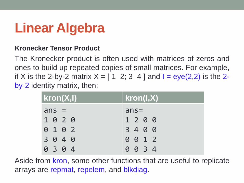
The Kronecker product is often used with matrices of zeros and
ones to build up repeated copies of small matrices. For example,
if X is the 2-by-2 matrix X = [ 1 2; 3 4 ] and I = eye(2,2) is the 2-
by-2 identity matrix, then:
Aside from kron, some other functions that are useful to replicate
arrays are repmat, repelem, and blkdiag.
kron(X,I) kron(I,X)
ans = 1 0 2 0 0 1 0 2 3 0 4 0 0 3 0 4
ans= 1 2 0 0 3 4 0 0 0 0 1 2 0 0 3 4
Linear Algebra
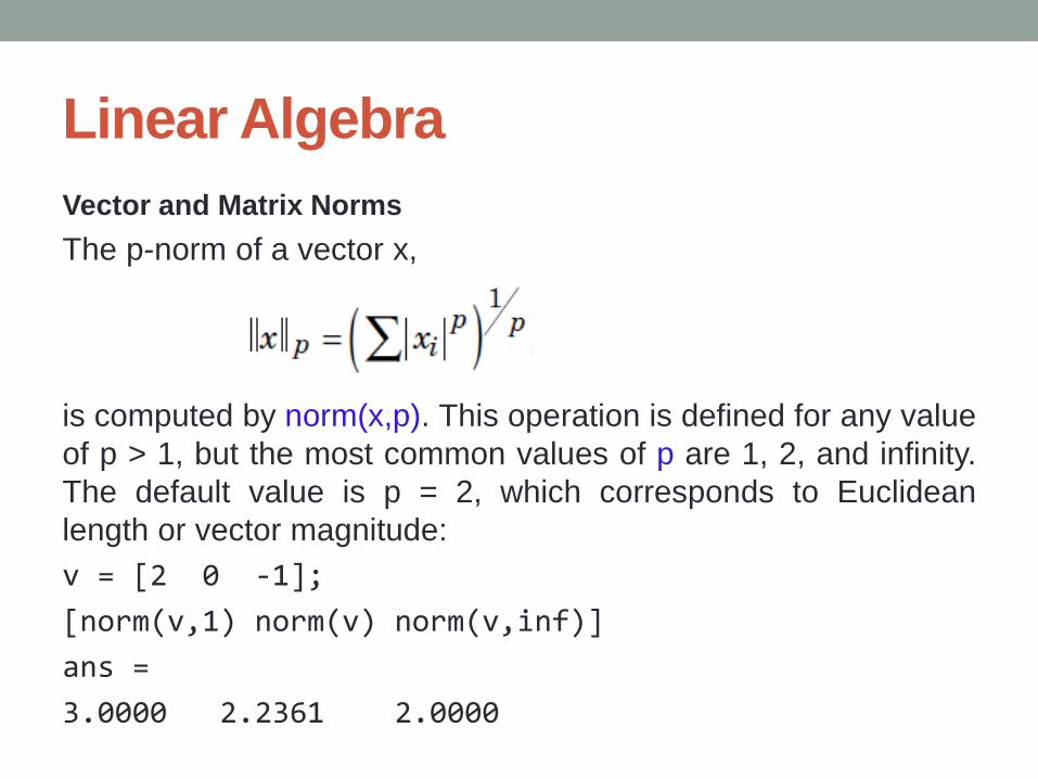
Vector and Matrix Norms
The p-norm of a vector x,
is computed by norm(x,p). This operation is defined for any value
of p > 1, but the most common values of p are 1, 2, and infinity.
The default value is p = 2, which corresponds to Euclidean
length or vector magnitude:
v = [2 0 -1];
[norm(v,1) norm(v) norm(v,inf)]
ans =
3.0000 2.2361 2.0000
Linear Algebra
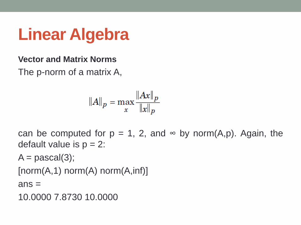
Vector and Matrix Norms
The p-norm of a matrix A,
can be computed for p = 1, 2, and ∞ by norm(A,p). Again, the
default value is p = 2:
A = pascal(3);
[norm(A,1) norm(A) norm(A,inf)]
ans =
10.0000 7.8730 10.0000

Linear Algebra
Vector and Matrix Norms
In cases where you want to calculate the norm of each row or
column of a matrix, you can use vecnorm:
vecnorm(A)
ans =
1.7321 3.7417 6.7823

Linear Algebra
Using Multithreaded Computation with Linear Algebra Functions
MATLAB supports multithreaded computation for a number of
linear algebra and element-wise numerical functions. These
functions automatically execute on multiple threads. For a
function or expression to execute faster on multiple CPUs, a
number of conditions must be true:
1 The function performs operations that easily partition into
sections that execute concurrently. These sections must be able
to execute with little communication between processes. They
should require few sequential operations.

Linear Algebra
Using Multithreaded Computation with Linear Algebra Functions
2) The data size is large enough so that any advantages of
concurrent execution outweigh the time required to partition the
data and manage separate execution threads. For example,
most functions speed up only when the array contains several
thousand elements or more.
3) The operation is not memory-bound; processing time is not
dominated by memory access time. As a general rule,
complicated functions speed up more than simple functions.
The matrix multiply (X*Y) and matrix power (X^p) operators show
significant increase in speed on large double-precision arrays
(on order of 10,000 elements). The matrix analysis functions det,
rcond, hess, and expm also show significant increase in speed
on large double-precision arrays.

Systems of Linear Equations
Computational Considerations
One of the most important problems in technical computing is
the solution of systems of simultaneous linear equations.In
matrix notation, the general problem takes the following form:
Given two matrices A and b, does there exist a unique matrix x,
so that Ax= b or xA= b?
It is instructive to consider a 1-by-1 example. For example, does
the equation
7x = 21
have a unique solution?
The answer, of course, is yes. The equation has the unique
solution x = 3. The solution is easily obtained by division:
x = 21/7 = 3.

Systems of Linear Equations
Computational Considerations
The solution is not ordinarily obtained by computing the inverse of 7,
that is 7–1= 0.142857..., and then multiplying 7–1 by 21. This would be
more work and, if 7–1 is represented to a finite number of digits, less
accurate.
Similar considerations apply to sets of linear equations with more than
one unknown; MATLAB solves such equations without computing the
inverse of the matrix.
Although it is not standard mathematical notation, MATLAB uses the
division terminology familiar in the scalar case to describe the solution
of a general system of simultaneous equations. The two division
symbols, slash, /, and backslash, \, correspond to the two MATLAB
functions mrdivide and mldivide. These operators are used for the two
situations where the unknown matrix appears on the left or right of the
coefficient matrix:

Systems of Linear Equations
Computational Considerations
These operators are used for the two situations where the unknown
matrix appears on the left or right of the coefficient matrix:
x = b/A Denotes the solution to the matrix equation
xA = b,obtained using mrdivide.
x = A\b Denotes the solution to the matrix equation
Ax = b,obtained using mldivide.
Think of “dividing” both sides of the equation Ax = b or xA = b by A. The
coefficient matrix A is always in the “denominator.”
Systems of Linear Equations
Computational Considerations
The dimension compatibility conditions for x = A\b require the two
matrices A and b to have the same number of rows.
The solution x then has the same number of columns as b and its row
dimension is equal to the column dimension of A. For x = b/A, the roles
of rows and columns are interchanged.
In practice, linear equations of the form Ax = b occur more frequently
than those of the form xA = b.
Consequently, the backslash is used far more frequently than the slash.
The remainder of this section concentrates on the backslash operator;
the corresponding properties of the slash operator can be inferred from
the identity:
(b/A)' = (A'\b').

Systems of Linear Equations
Computational Considerations
The coefficient matrix A need not be square. If A has size m-by-n, then
there are three cases:
m = n Square system. Seek an exact solution.
m > n Overdetermined system, with more equations than
unknowns. Find a least-squares solution.
m < n Underdetermined system, with fewer equations than
unknowns. Find a basic solution with at most m nonzero components.
The mldivide Algorithm
The mldivide operator employs different solvers to handle different
kinds of coefficient matrices. The various cases are diagnosed
automatically by examining the coefficient matrix.

Systems of Linear Equations
General Solution
The general solution to a system of linear equations Ax= b describes all
possible solutions. You can find the general solution by:
1) Solving the corresponding homogeneous system Ax = 0. Do
this using the null command, by typing null(A). This returns a basis for
the solution space to Ax = 0. Any solution is a linear combination of
basis vectors.
2) Finding a particular solution to the nonhomogeneous system
Ax =b.
You can then write any solution to Ax= b as the sum of the particular
solution to Ax =b, from step 2, plus a linear combination of the basis
vectors from step 1.
The rest of this section describes how to use MATLAB to find a
particular solution to Ax =b, as in step 2.

Systems of Linear Equations
Square Systems
The most common situation involves a square coefficient matrix A and
a single right-hand side column vector b.
Nonsingular Coefficient Matrix
If the matrix A is nonsingular, then the solution, x = A\b, is the same size
as b. For example:
A = pascal(3);
u = [3; 1; 4];
x = A\u
x =
10
-12
5

Systems of Linear Equations
Square Systems
It can be confirmed that A*x is exactly equal to u.
If A and b are square and the same size, x= A\b is also that size:
b = magic(3);
x = A\b
x =
19 -3 -1
-17 4 13
6 0 -6
It can be confirmed that A*x is exactly equal to b.
Both of these examples have exact, integer solutions. This is because
the coefficient matrix was chosen to be pascal(3), which is a full rank
matrix (nonsingular).

Systems of Linear Equations
Singular Coefficient Matrix
A square matrix A is singular if it does not have linearly independent
columns. If A is singular, the solution to Ax = b either does not exist, or
is not unique. The backslash operator, A\b, issues a warning if A is
nearly singular or if it detects exact singularity.
If A is singular and Ax = b has a solution, you can find a particular
solution that is not unique, by typing.
P = pinv(A)*b
pinv(A) is a pseudoinverse of A. If Ax = b does not have an exact
solution, then
pinv(A) returns a least-squares solution
Systems of Linear Equations
Singular Coefficient Matrix
For example:
A = [ 1 3 7
-1 4 4
1 10 18 ]
is singular, as you can verify by typing
rank(A)
ans =
2
Since A is not full rank, it has some singular values equal to zero.

Systems of Linear Equations
Singular Coefficient Matrix
Exact Solutions. For b =[5;2;12], the equation Ax = b has an exact
solution, given by
pinv(A)*b
ans =
0.3850
-0.1103
0.7066
Verify that pinv(A)*b is an exact solution by typing
A*pinv(A)*b
ans =
5.0000
2.0000
12.0000

Systems of Linear Equations
Singular Coefficient Matrix
Least-Squares Solutions. However, if b = [3;6;0], Ax = b does not have
an exact solution. In this case, pinv(A)*b returns a least-squares
solution. If you type
A*pinv(A)*b
ans =
-1.0000
4.0000
2.0000
you do not get back the original vector b.

Systems of Linear Equations
Singular Coefficient Matrix
You can determine whether Ax =b has an exact solution by finding the
row reduced echelon form of the augmented matrix [A b]. To do so for
this example, enter
rref([A b])
ans =
1.0000 0 2.2857 0
0 1.0000 1.5714 0
0 0 0 1.0000
Since the bottom row contains all zeros except for the last entry, the
equation does not have a solution. In this case, pinv(A) returns a least-
squares solution.

Systems of Linear Equations
Overdetermined Systems
This example shows how overdetermined systems are often
encountered in various kinds of curve fitting to experimental data.
A quantity, y, is measured at several different values of time, t, to
produce the following observations. You can enter the data and view it
in a table with the following statements.
t = [0 .3 .8 1.1 1.6 2.3]';
y = [.82 .72 .63 .60 .55 .50]';
B = table(t,y)
t y
0.0
0.3
0.8
1.1
1.6
2.3
0.82
0.72
0.63
0.6
0.55
0.5

Systems of Linear Equations
Overdetermined Systems
Try modeling the data with a decaying exponential function.
𝑦 𝑡 = 𝑐1+𝑐2𝑒−𝑡
The preceding equation says that the vector y should be approximated
by a linear combination of two other vectors. One is a constant vector
containing all ones and the other is the vector with components
exp(-t).
The unknown coefficients, 𝑐1 and 𝑐2, can be computed by doing a least-
squares fit, which minimizes the sum of the squares of the deviations of
the data from the model.

Systems of Linear Equations
Overdetermined Systems
There are six equations in two unknowns, represented by a 6-by-2
matrix.
E = [ones(size(t)) exp(-t)]
E = 6×2
1.0000 1.0000
1.0000 0.7408
1.0000 0.4493
1.0000 0.3329
1.0000 0.2019
1.0000 0.1003

Systems of Linear Equations
Overdetermined Systems
Use the backslash operator to get the least-squares solution.
c = E\y
c = 2×1
0.4760
0.3413
In other words, the least-squares fit to the data is
𝑦 𝑡 = 0.4760+034313𝑒−𝑡
The following statements evaluate the model at regularly spaced
increments in t, and then plot the result together with the original data:
T = (0:0.1:2.5)';
Y = [ones(size(T)) exp(-T)]*c;
plot(T,Y,'-',t,y,'o')

Systems of Linear Equations
Graphs of table data and 𝑦 𝑡 = 0.4760+034313𝑒−𝑡

Systems of Linear Equations
Overdetermined Systems
E*c is not exactly equal to y, but the difference might well be less
than measurement errors in the original data.
A rectangular matrix A is rank deficient if it does not have linearly
independent columns.
If A is rank deficient, then the least-squares solution to AX = B is not
unique. A\B issues a warning if A is rank deficient and produces a
least-squares solution.
You can use lsqminnorm to find the solution X that has the minimum
norm among all solutions.

Systems of Linear Equations
Underdetermined Systems
This example shows how the solution to underdetermined systems is not
unique. Underdetermined linear systems involve more unknowns than
equations. The matrix left division operation in MATLAB finds a basic least-
squares solution, which has at most m nonzero components for an m-by-n
coefficient matrix. Here is a small, random example:
R = [6 8 7 3; 3 5 4 1]
rng(0);
b = randi(8,2,1)
R =
6 8 7 3
3 5 4 1
b =
7
8

Systems of Linear Equations
Underdetermined Systems
The linear system Rp = b involves two equations in four
unknowns. Since the coefficient matrix contains small integers, it
is appropriate to use the format command to display the solution
in rational format. The particular solution is obtained with
format rat %numbers in rational format
p = R\b
p =
0
17/7
0
-29/7

Systems of Linear Equations
Underdetermined Systems
One of the nonzero components is p(2) because R(:,2) is the column of
R with largest norm. The other nonzero component is p(4) because
R(:,4) dominates after R(:,2) is eliminated.
The complete general solution to the underdetermined system can be
characterized by adding p to an arbitrary linear combination of the null
space vectors, which can be found using the null function with an
option requesting a rational basis.
Z = null(R,'r')
Z =
-1/2 -7/6
-1/2 1/2
1 0
0 1

Systems of Linear Equations
Underdetermined Systems
It can be confirmed that R*Z is zero and that the residual R*x - b is
small for any vector:
x, where
x = p + Z*q
Since the columns of Z are the null space vectors, the product Z*q is a
linear combination
of those vectors:

Systems of Linear Equations
Underdetermined Systems
To illustrate, choose an arbitrary q and construct x.
q = [-2; 1];
x = p + Z*q;
Calculate the norm of the residual.
format short
norm(R*x - b)
ans =
2.6645e-15

Systems of Linear Equations
Underdetermined Systems
When infinitely many solutions are available, the solution with minimum
norm is of particular interest. You can use lsqminnorm to compute the
minimum-norm leastsquares solution. This solution has the smallest
possible value for norm(p).
p = lsqminnorm(R,b)
p =
-207/137
365/137
79/137
-424/137

Systems of Linear Equations
Solving for Several Right-Hand Sides
Some problems are concerned with solving linear systems that have
the same coefficient matrix A, but different right-hand sides b. When the
different values of b are available at the same time, you can construct b
as a matrix with several columns and solve all of the systems of
equations at the same time using a single backslash command:
X = A\[b1 b2 b3 …].
However, sometimes the different values of b are not all available at the
same time, which means you need to solve several systems of
equations consecutively. When you solve one of these systems of
equations using slash (/) or backslash (\), the operator factorizes the
coefficient matrix A and uses this matrix decomposition to compute the
solution. However, each subsequent time you solve a similar system of
equations with a different b, the operator computes the same
decomposition of A, which is a redundant computation.
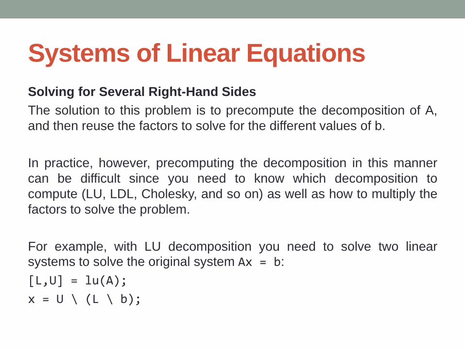
Systems of Linear Equations
Solving for Several Right-Hand Sides
The solution to this problem is to precompute the decomposition of A,
and then reuse the factors to solve for the different values of b.
In practice, however, precomputing the decomposition in this manner
can be difficult since you need to know which decomposition to
compute (LU, LDL, Cholesky, and so on) as well as how to multiply the
factors to solve the problem.
For example, with LU decomposition you need to solve two linear
systems to solve the original system Ax = b:
[L,U] = lu(A);
x = U \ (L \ b);
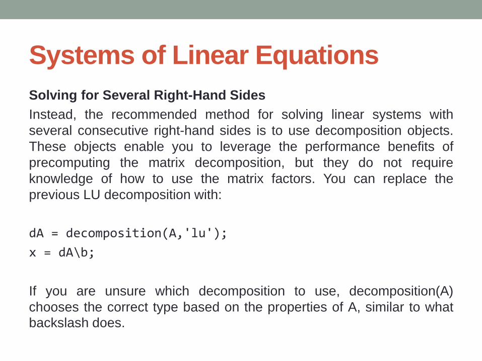
Systems of Linear Equations
Solving for Several Right-Hand Sides
Instead, the recommended method for solving linear systems with
several consecutive right-hand sides is to use decomposition objects.
These objects enable you to leverage the performance benefits of
precomputing the matrix decomposition, but they do not require
knowledge of how to use the matrix factors. You can replace the
previous LU decomposition with:
dA = decomposition(A,'lu');
x = dA\b;
If you are unsure which decomposition to use, decomposition(A)
chooses the correct type based on the properties of A, similar to what
backslash does.

Systems of Linear Equations
Solving for Several Right-Hand Sides
n = 1e3;
A = sprand(n,n,0.2) + speye(n); b = ones(n,1);
% Backslash solution
tic
for k = 1:100
x = A\b;
end
toc
Elapsed time is 9.006156 seconds.
For this problem, the decomposition solution is much faster than using
backslash alone, yet the syntax remains simple.

Systems of Linear Equations
Solving for Several Right-Hand Sides
Here is a simple test of the possible performance benefits of this
approach. The test solves the same sparse linear system 100 times
using both backslash (\) and decomposition.
% decomposition solution
tic
dA = decomposition(A);
for k = 1:100
x = dA\b;
end
toc
Elapsed time is 0.374347 seconds.


![MATLAB matrices [ ]](https://img.pdfslide.us/doc/110x75/62163616ceb768082917a488/matlab-matrices-.jpg)


