MATLAB® in Bioscience

and Biotechnology

Volumes in the Series

1. Clinical Research in Asia. U. Sahoo (ISBN 9781907568008).

2. Outsourcing Biopharma R&D to India. P. R. Chowdhury (ISBN 9781907568084).

3. Practical Leadership for Biopharmaceutical Executives. J. Chin (ISBN 9781907568060)

4. A Biotech Manager’s Handbook. M. O’Neill (ed.) (ISBN 9781907568145).

5. RNA Interference. T. Novobrantseva et al. (ISBN 9781907568169).

6. Therapeutic Protein Formulation. B. Meyer (ed.) (ISBN 9781907568183).

7. Patent Litigation in the Pharmaceutical and Biotechnology Industries. G. Morgan (ISBN 9781907568206).

8. Matlab® in Bioscience and Biotechnology. L. Burstein (ISBN 9781907568046).

9. Clinical Research in Paediatric Psychopharmacology. P. Auby (ISBN 9781907568244).

10. Concepts and Techniques in Genomics and Proteomics. N. Saraswathy and P. Ramalingam (ISBN 9781907568107).

11. An Introduction to Biotechnology. W. T. Godbey (ISBN 9781907568282).

12. The Application of SPC in the Pharmaceutical and Biotechnology

Industries. T. Cochrane (ISBN 9781907568336).

13. Patently Innovative: How Pharmaceutical Firms Use Emerging Patent Law to Extend Monopolies on Blockbuster Drugs. R. Bouchard (ISBN 9781907568121).

14. Therapeutic Antibody Engineering. W. R. Strohl and L. M. Strohl (ISBN 9781907568374).

15. Ultrafiltration for Bioprocessing. H. Lutz (ISBN 9781907568466).

16. Therapeutic Risk Management of Medicines. A. K. Banerjee (ISBN 9781907568480).

17. 21st Century Quality Management and Good Management Practices: Value Added Compliance for the Pharmaceutical and Biotechnology Industry. S. Williams (ISBN 9781907568503).

18. An Introduction to Pharmaceutical Sciences. J. Roy (ISBN 9781907568527).

19. Pharmaceutical Licenses: Valuation and Execution. S. Mayhew and I. Walker (ISBN 9781907568565).

20. CAPA in the Pharmaceutical and Biotech Industries. J. Rodriguez (ISBN 9781907568589).

21. Commercialising the Stem Cell Sciences. O. Harvey (ISBN 9781907568602).

22. Process Validation for the Production of Biopharmaceuticals: Principles and Best Practice. Applied Strategies for Bioprocess Development and

Biohealthcare Publishing Series on Pharma, Biotech and Biosciences: Science, Technology and Business

Volumes in the Series

1. Medical Education, Training and Care Delivery in a Virtual World. K. Kahol (ISBN 9781907568039).

2. Allergens and Respiratory Pollutants. M. Williams (ed.) (ISBN 9781907568541).

Biohealthcare Publishing Series on Medical and Health Science, Technology and Policy

Volumes in the Series

1. In Silico Protein Design. C. M. Frenz (ISBN 9781907568268).

2. Bioinformatics for Computer Science. K. Revett (ISBN 9781907568329).

3. Gene Expression Analysis in the RNA World. J. Q. Clement (ISBN 9781907568305).

4. Computational Methods for Finding Inferential Bases in Molecular Genetics. Q.-N. Tran (ISBN 9781907568398).

5. Computer-Aided Vaccine Design. T. J. Chuan and S. Ranganathan (ISBN 9781907568411).

6. Bioinformatics for Biomedical Science and Clinical Applications. K.-H. Liang (ISBN 9781907568442).

7. Deterministic Versus Stochastic Modelling in Biochemistry and Systems Biology. P. Lecca et al. (ISBN 9781907568626).

Biohealthcare Publishing Series on Bioinformatics

Manufacture. A. Newcombe et al. (ISBN 9781907568640).

23. Clinical Trial Management. An Overview. A. U. Sahoo et al. (ISBN 9781907568664).

24. Annotating New Genes: From In Silico to Validations by Experiments. S. Uchida (ISBN 9781907568688).

25. Impact of Regulation on Drug Development. H. Guenter Hennings (ISBN 9781907568701).

26. The Design and Manufacture of Medical Devices. J. Paulo Davim (ISBN 9781907568725).

MATLAB® in Bioscience and Biotechnology

Leonid Burstein

Biohealthcare Publishing (Oxford) Limited

Hexagon House Avenue 4 Station Lane WitneyOxford OX28 4BN, UKTel: +44 (0) 1993 848726; Fax: +44 (0) 1865 884448 Email: info@biohealthcarepublishing.com Website: www.biohealthcarepublishing.com

First published in 2011 by Biohealthcare Publishing (Oxford) Limited ISBNs: 978 1 907568 04 6 (print) and 978 1 908818 03 4 (e-book)

© L. Burstein, 2011

The right of L. Burstein to be identified as author of this Work has been asserted by him in accordance with sections 77 and 78 of the Copyright, Designs and Patents Act 1988.

British Library Cataloguing-in-Publication Data: a catalogue record for this book is available from the British Library.

All rights reserved. No part of this publication may be reproduced, stored in or introduced into a retrieval system, or transmitted, in any form, or by any means (electronic, mechanical, photocopying, recording or otherwise) without the prior written permission of the Publishers. This publication may not be lent, resold, hired out or otherwise disposed of by way of trade in any form of binding or cover other than that in which it is published without the prior consent of the Publishers. Any person who does any unauthorised act in relation to this publication may be liable to criminal prosecution and civil claims for damages.

Permissions may be sought directly from the Publishers, at the above address.

The use in this publication of trade names, trademarks, service marks, and similar terms, even if they are not identified as such, is not to be taken as an expression of opinion as to whether or not they are subject to proprietary rights. The Publishers are not associated with any product or vendor mentioned in this publication.

The authors, editors, contributors and Publishers have attempted to trace the copyright holders of all material reproduced in this publication and apologise to any copyright holders if permission to publish in this form has not been obtained. If any copyright material has not been acknowledged, please write and let us know so we may rectify in any future reprint. Any screenshots in this publication are the copyright of the website owner(s), unless indicated otherwise.

Limit of Liability/Disclaimer of WarrantyThe Publishers, author(s), editor(s) and contributor(s) make no representations or warranties with respect to the accuracy or completeness of the contents of this publication and specifically disclaim all warranties, including without limitation warranties of fitness for a particular purpose. No warranty may be created or extended by sales or promotional materials. The advice and strategies contained herein may not be suitable for every situation. This publication is sold with the understanding that the Publishers are not rendering legal, accounting or other professional services. If professional assistance is required, the services of a competent professional person should be sought. No responsibility is assumed by the Publishers, author(s), editor(s) or contributor(s) for any loss of profit or any other commercial damages, injury and/or damage to persons or property as a matter of products liability, negligence or otherwise, or from any use or operation of any methods, products, instructions or ideas contained in the material herein. The fact that an organisation or website is referred to in this publication as a citation and/or potential source of further information does not mean that the Publishers nor the author(s), editor(s) and contributor(s) endorses the information the organisation or website may provide or recommendations it may make. Further, readers should be aware that internet websites listed in this work may have changed or disappeared between when this publication was written and when it is read. Because of rapid advances in medical sciences, in particular, independent verification of diagnoses and drug dosages should be made.

Typeset by Domex e-Data Pvt. Ltd.Printed in the UK and USA Cover design by Hutchins Creative

MATLAB, Bioinformatics toolbox and Simulink are registered trademarks of The MathWorks, Inc.

In memory of my father Matvey.To my mother Leda, my wife Inna, and my son Dmitri

Contents

Preface xiList of figures and tables xiiiAbout the author xvii

1 Introduction 1

2 MATLAB® basics 3

2.1 Starting with MATLAB® 3 2.2 Vectors, matrices and arrays 15 2.3 Flow control 33 2.4 Questions for self-checking and exercises 44 2.5 Answers to selected exercises 48

3 MATLAB® graphics 49

3.1 Generation of XY plots 49 3.2 Generation of XYZ plots 62 3.3 Specialized 2D and 3D plots 73 3.4 Application examples 79 3.5 Questions for self-checking and exercises 88 3.6 Answers to selected exercises 93

4 Script, function files and some useful MATLAB® functions 95

4.1 Script file 95 4.2 Functions and function files 100 4.3 Some useful MATLAB® functions 104 4.4 Application examples 116 4.5 Questions for self-checking and exercises 127 4.6 Answers to selected exercises 129

x MATLAB® in Bioscience and Biotechnology

5 Ordinary and partial differential equation solvers 133

5.1 Solving ordinary differential equations with ODE solvers 133 5.2 Solving partial differential equations with the PDE solver 151 5.3 Questions for self-checking and exercises 162 5.4 Answers to selected exercises 167

6 Bioinformatics tool for sequence analysis 171

6.1 About toolboxes 171 6.2 The functions of the Bioinformatics toolbox™ 172 6.3 Public databases, data formats and commands for their management 173 6.4 Sequence analysis 182 6.5 Sequence analysis examples 197 6.6 Questions for self-checking and exercises 209 6.7 Answers to selected exercises 211

Appendix: MATLAB® characters, operators and commands 217

Index 223

Preface

In the last few decades, two seemingly disparate sciences – computer science and biology – have interpenetrated and affected one another. We see students enrolled in computer science beginning their careers in biotechnological laboratories, and biotechnologists creating bio-computers and being active in computer science. There appears to be an urgent need to familiarize biotechnologists with the same computing tools as are imparted to technicians.

This book represents a short introduction to MATLAB® oriented towards various collaborative areas of biotechnology and bioscience. My hope is that it will be equally useful to undergraduate and graduate students and to practising engineers. It concentrates on the fundamentals of MATLAB® and gives examples of its application to a wide range of current bioengineering problems in computational biology, molecular biology, biokinetics, biomedicine, bioinformatics and biotechnology. In the last decade MATLAB® has been presented to students as a basic computational tool that they need to learn. Consequently, many students unfamiliar with programming, engineers and scientists have come to regard it as user-friendly and highly convenient in solving their specific problems. Numerous books are available on programming in MATLAB® for engineers in general, irrespective of their specialization, or for those specializing in some specific area, but none has been designed specifically for a wide, interdisciplinary, topical area such as bioengineering. Thus, MATLAB® is presented here with examples and applications to various school- and advanced bioengineering problems – from growing populations of microorganisms and population dynamics, to reaction kinetics and reagent concentrations, predator–prey models, mass-transfer problems, and to sequence analysis and sequence statistics.

The book distills my experience of many years of MATLAB® teaching in introductory and advanced courses for students, engineers and scientists specializing in bioscience and engineering.

I would like to thank the people who attracted me to the subject and thereby played key roles in the inception and appearance of this book: my

xii MATLAB® in Bioscience and Biotechnology

colleague Professor Rosa Azhari (Biotechnology Department, ORT Braude College), and software support team head Moshe Barak (Computer Center, Technion – Israel Institute of Technology). I also thank MathWorks Inc. (3 Apple Hill Drive, Natick, MA 01760-2098, USA, Tel: 508-647-7000, Fax: 508-647-7001, E-mail: info@mathworks.com, Web: www.mathworks.com) who graciously granted permission to reproduce material appearing in this book.

I thank Ing. Eliezer Goldberg, former resident scientific editor at Technion, for patience and invaluable editorial assistance, and would also like to thank Dr Glyn Jones, head of Biohealthcare Publishing (Oxford) Ltd, for invaluable support throughout all stages of publication of this book.

I hope this book will prove useful to students and engineers in both natural and life sciences and provide them with an opportunity to work with one of the finest software tools.

Any reports of errata or bugs, comments and suggestions on the book’s contents will be accepted gratefully by the author.

Leonid BursteinNesher, Haifa, Karmiel, IsraelSeptember 2010

List of figures and tables

Figures

2.1 MATLAB® logo. The image can be produced with the logo command; the background color has been changed 4

2.2 MATLAB® desktop 4

2.3 Command Window; the view after separation from the desktop 6

2.4 Help window with information about the aminolookup command 9

3.1 Biomass data plotted in the Figure Window with default settings 50

3.2 Biomass data generated with specifiers and property settings in the plot command 52

3.3 Two curves (sine and cosine) in a single plot 54

3.4 sin x, cos x and sin x2 in a single plot 54

3.5 Possible arrangements of one page in four panes 55

3.6 Four plots on the same page 56

3.7 Sine and cosine plot constructed with the axis tight command 58

3.8 Biomass data plot formatted with the xlabel, ylabel, title, text and grid commands 60

3.9 Plot of the sine and cosine functions with legend 61

3.10 Plot Editor buttons in the Figure Window 62

3.11 Line in 3D coordinates 64

xiv MATLAB® in Bioscience and Biotechnology

3.12 Points in 3D interpretation and their x,y-plane projection 65

3.13 Mesh plot 67

3.14 Surface plot 68

3.15 Boxed surface plot 69

3.16 Viewpoint, azimuth and elevation 70

3.17 The function z = e–x2–y2 with viewing angles 71

3.18 Plot in rotation regime with the rotate cursor and values of azimuth and elevation angles 72

3.19 Plot of biomass–time data with error bars 74

3.20 Histogram of the weight data 75

3.21 Semi-logarithmic graph for the relationship between time elapsed and residual radioactivity 76

4.1 The Editor Window 96

4.2 Script file in the Editor Window 97

4.3 The ‘Current Folder’ field and ‘Browse for Folder’ Window 98

4.4 Typical function file in the Editor Window 101

4.5 Original data, interpolation and extrapolation points 105

4.6 Definite integral of the function f(x) given analytically and by the data points 108

4.7 Geometrical representation of the derivative 111

4.8 First-degree polynomial fit 115

5.1 Concentration–time dependence for second-order

reaction; the solution to − =dd[ ]

[ ]At

k A 2, with A0 = 0.25 138

5.2 Concentration–coordinate–time dependences; the

solution to ∂

∂=

∂

∂

ut

Du

x

2

2 . The level values were replaced

with the Plot Editor

156

6.1 Matlab® Web Browser with NCBI home page 176

6.2 The page with accession number for rat hexosaminidase A 177

List of figures and tables xv

6.3 Bar chart of amino acid amounts produced by the aacount command for a randomly generated 25-letter sequence 186

6.4 A, C, G, T and A, T, C, G nucleotide density plots generated by the ntdensity command for the rhesus macaque semen sequence 187

6.5 Sequence score example 190

6.6 Scoring space heat map and winning path generated with the nwalign command 192

6.7 Scoring space heat map and winning path generated with the swalign command 193

6.8 Dot plot for mouse and rat hexoaminidase A sequences, generated by the seqdotplot command 195

6.9 Aligned Sequence window generated by the showalignment command; pairwise alignment 196

6.10 Aligned Sequence window generated by the showalignment command; multiple alignment 196

6.11 Multiple Sequence Alignment Viewer with four aligned sequences generated with the multialignviewer command 198

Tables

2.1 Elementary and trigonometric mathematical functions 7

2.2 Biomass data 15

2.3 Enzyme activity (mg–1) 17

2.4 Command for matrix manipulations, generation and analysis 26

2.5 If statements 37

2.6 Loops 38

3.1 Line style, color and marker type specifiers 51

3.2 Property names and property values 51

xvi MATLAB® in Bioscience and Biotechnology

3.3 Additional commands and plots for 2D and 3D graphics 77

3.4 Air temperature–density data 84

5.1 MATLAB® ODE solvers 135

6.1 Additional commands for database management 179

6.2 Additional utility and statistical commands 188

About the author

Leonid Burstein is Senior Lecturer at large at Technion – Israel Institute of Technology, at the ORT Braude College, in the Biotechnology and Software Engineering Departments, and at a number of other universities and highschools in Western and Lower Galilee.

Following an MA in thermophysics at Lomonosov Technological Institute at Odessa, Ukraine, and a doctorate at the National Research Institute for Physical and Radio Engineering Measurements at Moscow, he obtained his PhD in physical properties of materials from the Heat/Mass Transfer Institute of the Belarus Academy of Science, Minsk, in 1974. After a short period of work in Russia and Belarus, Dr Burstein started his carrier at the Piston Ring Institute in Odessa, where he served from 1974 to 1990 as Head of Projects and Head of the CAD/CAM group. In 1991, he began work at the Technion – IIT, Israel, at the Faculty of Mechanical Engineering, in the Quality Assurance and Reliability Program at the Faculty of Industrial Engineering and Management, and at the Taub Computer Centre as an advisor on MATLAB® and other scientific software. He also worked at the Technion Research and Development Foundation as principal researcher in funded projects in various areas such as diesel tribology and environment control. He also taught various courses at Haifa University, at the Technion, at the Kinnereth Academic College and elsewhere. He currently teaches a MATLAB® course for biotechnologists at ORT Braude College.

He is an Editorial Board Member and reviewer for a number of international journals and a Committee Member of numerous conferences. He is the author of several patents, has published four chapters in scientific books and authored/co-authored more than 60 publications in leading scientific journals.

xviii MATLAB® in Bioscience and Biotechnology

He can be contacted at:

Technion – Israel Institute of TechnologyTechnion City32000 HaifaIsraelE-mail: leonidburstein@gmail.com (prefereble) or leonidb@technion.ac.il

1

Introduction

Everything that can be counted – should be. Anonymous

Biological engineering is defined as application of engineering principles to the widest spectrum of living systems – from molecular biology, biochemistry and microbiology, to bio-medicine, genetics and bioinformatics. And as in general engineering, computers and the ability to use them are vitally important. This is true also for other professionals of any bio-industry. Thus, bio-specialists and scientists working in these areas need to have the computational resources to be able to solve various problems. A widespread and powerful tool for such purposes is MATLAB® – the software for technical computing. It is designed to solve both general and specific problems; of these, the latter are treated with so-called toolboxes, which currently include means specialized for bio-problems. An obstacle to the effective understanding and implementation of MATLAB® in practice is the inadequate level of math reached by students and specialists in areas of bioscience, combined with a lack of textbooks tailored to such audiences. This book is intended as a remedy. It is organized as follows.

I begin by covering primary MATLAB® programming and then move to more complicated problems by means of this language; the material is illustrated throughout by examples from different areas of bioengineering and biological science. The topics were chosen on the basis of several years of teaching MATLAB® for biotechnologists and they are presented so that inexperienced users can progress gradually, with the previously presented material being the only prerequisite for each new chapter.

Chapter 2 introduces the MATLAB® environment, language design, help options, variables, matrix and array manipulations, elementary and special functions, flow chart control, conditional statements and other basic MATLAB® features.

2 MATLAB® in Bioscience and Biotechnology

In chapter 3 the plotting tool is described by using examples of graphic presentation in various calculations. Mastering the material in chapters 2 and 3 will allow readers to create their own MATLAB® programs.

Chapter 4 presents the MATLAB® script- and m-files; the commands for numerical integration, differentiation, inter-/extrapolation and curve fitting, together with their various applications, are given.

In chapter 5, particular solutions for ordinary and partial differential equations are briefly presented together with examples from bio-systems involving a single differential equation or a set. This chapter assumes a somewhat greater familiarity with mathematics.

In the final chapter the bioinformatics tool is introduced through applications employed in sequence analysis and statistics. Emphasis is placed on DNA and protein sequence database access and further pairwise or multiple alignments.

The Appendix details the studied MATLAB® commands and functions.Application problems included at the end (and sometimes in the middle)

of each chapter are solved with commands accessible to the reader; the solutions are not necessarily the shortest or most original, but should be easy to understand and follow up. Readers are invited to write their own solutions and check the results against those given herein. At the end of each chapter are questions and problems, and readers are encouraged to attempt them for better assimilation of the material. The contexts and values used in the problems are not factual and are intended for learning purposes only.

The MATLAB® used in the book is R2010a, version 7.10.0. Each subsequent version should incorporate all previous ones; hence, the fundamental commands given here should be valid in future versions. It is assumed that the user has a computer with MATLAB® installed on it and is able to perform basic computer operations.

Each command is explained here in its simplest form; additional information is available in the MATLAB®-help or original MATLAB® documentation.

Let us begin.

2

MATLAB® basics

MATLAB® came into being in the 1970s as a tool for mathematicians and educators, but was soon adopted by engineers as an effective means for technical computing. Its name is a composite of the words ‘Matrix’ and ‘Laboratory’, emphasizing that its main element is the matrix. Such an approach permitted unification of the processes of various calculations, graphics, modeling, simulation and algorithm development. This chapter introduces the main windows and starting procedure, describes the main commands for simple arithmetic, algebraic and matrix operations, and presents the basic loops and relational and logical operators.

2.1 Starting with MATLAB®

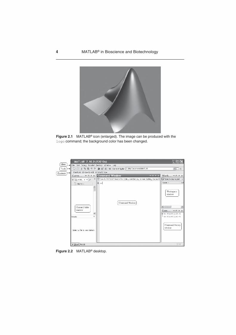
MATLAB® can be installed on computers running different operation systems, but I will assume here that the reader uses a personal computer running a Windows operating system. To start one has simply to click on the MATLAB® icon (Figure 2.1) provided with a MATLAB® subscription; the icon is placed on the Quick Lunch bar or on the Windows Desktop. Another way to start the program is to select MATLAB® 20010a in the MATLAB®-directory in the ‘All Programs’ option of the Windows ‘Start’ menu.

2.1.1 MATLAB® Desktop and its windows

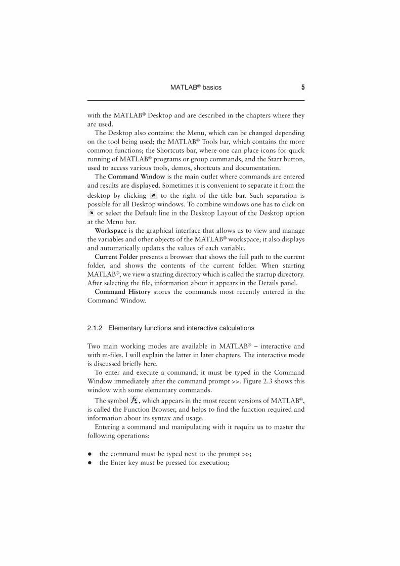
The window that first opens is the MATLAB® Desktop (Figure 2.2), which comprises four windows: Command, Current Folder, Workspace and Command History.

These are the most intensively used windows and are briefly described further. There are also Help, Editor and Figure windows that do not appear

4 MATLAB® in Bioscience and Biotechnology

Figure 2.1 MATLAB® icon (enlarged). The image can be produced with the logo command; the background color has been changed.

Figure 2.2 MATLAB® desktop.

MATLAB® basics 5

with the MATLAB® Desktop and are described in the chapters where they are used.

The Desktop also contains: the Menu, which can be changed depending on the tool being used; the MATLAB® Tools bar, which contains the more common functions; the Shortcuts bar, where one can place icons for quick running of MATLAB® programs or group commands; and the Start button, used to access various tools, demos, shortcuts and documentation.

The Command Window is the main outlet where commands are entered and results are displayed. Sometimes it is convenient to separate it from the

desktop by clicking to the right of the title bar. Such separation is possible for all Desktop windows. To combine windows one has to click on

or select the Default line in the Desktop Layout of the Desktop option at the Menu bar.

Workspace is the graphical interface that allows us to view and manage the variables and other objects of the MATLAB® workspace; it also displays and automatically updates the values of each variable.

Current Folder presents a browser that shows the full path to the current folder, and shows the contents of the current folder. When starting MATLAB®, we view a starting directory which is called the startup directory. After selecting the file, information about it appears in the Details panel.

Command History stores the commands most recently entered in the Command Window.

2.1.2 Elementary functions and interactive calculations

Two main working modes are available in MATLAB® – interactive and with m-files. I will explain the latter in later chapters. The interactive mode is discussed briefly here.

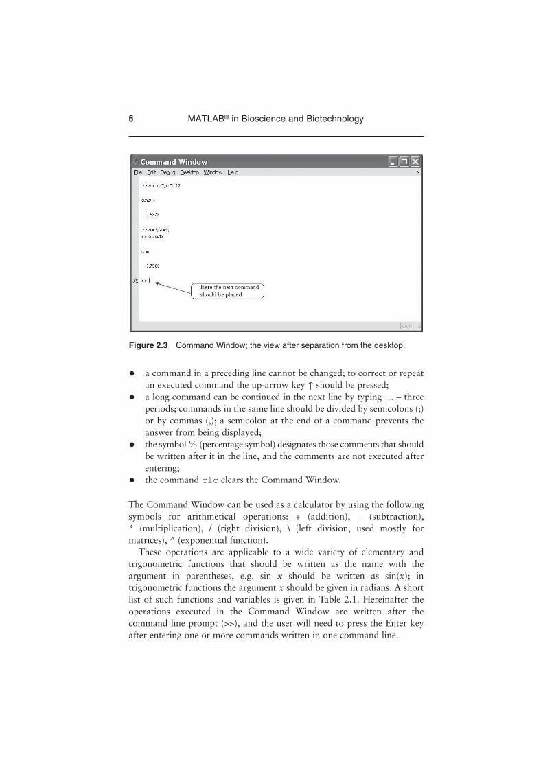
To enter and execute a command, it must be typed in the Command Window immediately after the command prompt >>. Figure 2.3 shows this window with some elementary commands.

The symbol , which appears in the most recent versions of MATLAB®, is called the Function Browser, and helps to find the function required and information about its syntax and usage.

Entering a command and manipulating with it require us to master the following operations:

the command must be typed next to the prompt >>; •the Enter key must be pressed for execution; •

6 MATLAB® in Bioscience and Biotechnology

a command in a preceding line cannot be changed; to correct or repeat •an executed command the up-arrow key ↑ should be pressed; a long command can be continued in the next line by typing … – three •periods; commands in the same line should be divided by semicolons (;) or by commas (,); a semicolon at the end of a command prevents the answer from being displayed;the symbol % (percentage symbol) designates those comments that should •be written after it in the line, and the comments are not executed after entering; the command • clc clears the Command Window.

The Command Window can be used as a calculator by using the following symbols for arithmetical operations: + (addition), – (subtraction), * (multiplication), / (right division), \ (left division, used mostly for matrices), ^ (exponential function).

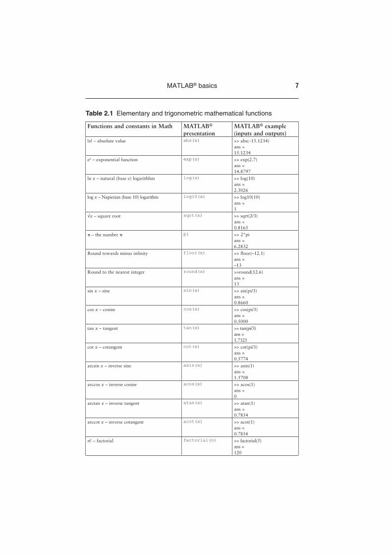
These operations are applicable to a wide variety of elementary and trigonometric functions that should be written as the name with the argument in parentheses, e.g. sin x should be written as sin(x); in trigonometric functions the argument x should be given in radians. A short list of such functions and variables is given in Table 2.1. Hereinafter the operations executed in the Command Window are written after the command line prompt (>>), and the user will need to press the Enter key after entering one or more commands written in one command line.

Figure 2.3 Command Window; the view after separation from the desktop.

MATLAB® basics 7

Functions and constants in Math MATLAB® presentation

MATLAB® example (inputs and outputs)

|x| – absolute value abs(x) >> abs(–15.1234) ans = 15.1234

ex – exponential function exp(x) >> exp(2.7) ans = 14.8797

ln x – natural (base e) logarithhm log(x) >> log(10) ans = 2.3026

log x – Napierian (base 10) logarithm log10(x) >> log10(10) ans = 1

√x – square root sqrt(x) >> sqrt(2/3) ans = 0.8165

p – the number p pi >> 2*pi ans = 6.2832

Round towards minus infinity floor(x) >> floor(–12.1) ans = –13

Round to the nearest integer round(x) >>round(12.6) ans = 13

sin x – sine sin(x) >> sin(pi/3) ans = 0.8660

cos x – cosine cos(x) >> cos(pi/3) ans = 0.5000

tan x – tangent tan(x) >> tan(pi/3) ans = 1.7321

cot x – cotangent cot(x) >> cot(pi/3) ans = 0.5774

arcsin x – inverse sine asin(x) >> asin(1) ans = 1.5708

arccos x – inverse cosine acos(x) >> acos(1) ans = 0

arctan x – inverse tangent atan(x) >> atan(1) ans = 0.7854

arccot x – inverse cotangent acot(x) >> acot(1) ans = 0.7854

n! – factorial factorial(n) >> factorial(5) ans = 120

Table 2.1 Elementary and trigonometric mathematical functions

8 MATLAB® in Bioscience and Biotechnology

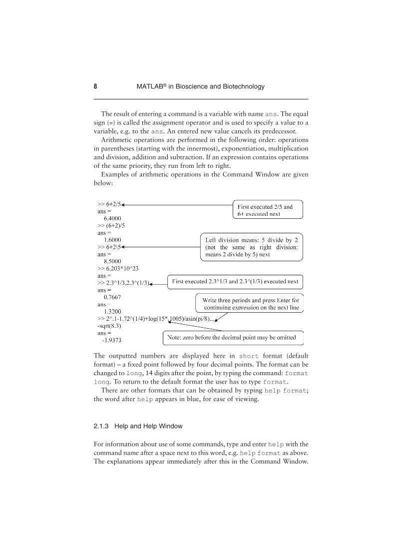
The result of entering a command is a variable with name ans. The equal sign (=) is called the assignment operator and is used to specify a value to a variable, e.g. to the ans. An entered new value cancels its predecessor.

Arithmetic operations are performed in the following order: operations in parentheses (starting with the innermost), exponentiation, multiplication and division, addition and subtraction. If an expression contains operations of the same priority, they run from left to right.

Examples of arithmetic operations in the Command Window are given below:

The outputted numbers are displayed here in short format (default format) – a fixed point followed by four decimal points. The format can be changed to long, 14 digits after the point, by typing the command: format long. To return to the default format the user has to type format.

There are other formats that can be obtained by typing help format; the word after help appears in blue, for ease of viewing.

2.1.3 Help and Help Window

For information about use of some commands, type and enter help with the command name after a space next to this word, e.g. help format as above. The explanations appear immediately after this in the Command Window.

MATLAB® basics 9

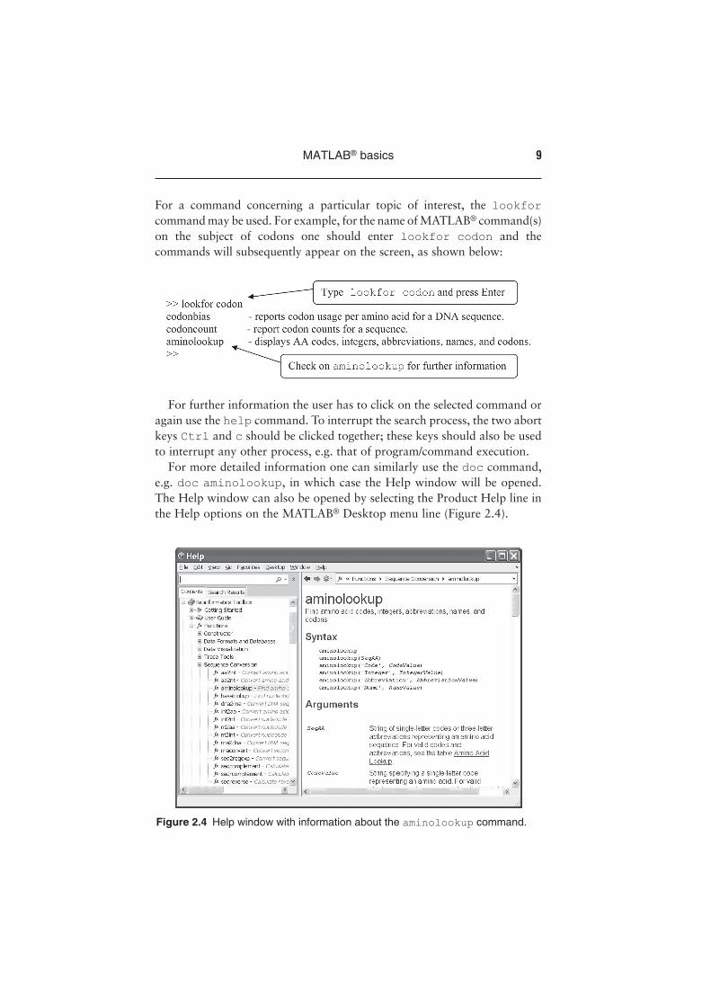
For a command concerning a particular topic of interest, the lookfor command may be used. For example, for the name of MATLAB® command(s) on the subject of codons one should enter lookfor codon and the commands will subsequently appear on the screen, as shown below:

For further information the user has to click on the selected command or again use the help command. To interrupt the search process, the two abort keys Ctrl and c should be clicked together; these keys should also be used to interrupt any other process, e.g. that of program/command execution.

For more detailed information one can similarly use the doc command, e.g. doc aminolookup, in which case the Help window will be opened. The Help window can also be opened by selecting the Product Help line in the Help options on the MATLAB® Desktop menu line (Figure 2.4).

Figure 2.4 Help window with information about the aminolookup command.

10 MATLAB® in Bioscience and Biotechnology

The Help window comprises three panes: on the left are the Contents or Search Results and on the right is the page containing information on the topic. Information on any subject is obtainable by typing the word(s) into the search line in the upper left-hand corner. The Search Results pane shows a preview of where the search words were found within the page, and the concrete information is displayed on the right.

2.1.4 Variables and commands for management of variables

A variable is a symbolic term written as a letter(s) and associated with a concrete numerical value. MATLAB® allocates memory space for storage of variable names and their values. A variable can be a scalar – a single number – or an array – a table of numbers. The name can be as many as 63 characters long, and contain letters, digits and underscores, but the first character must be a letter. Existing commands (sin, cos, sqrt, etc.) cannot be used as names.

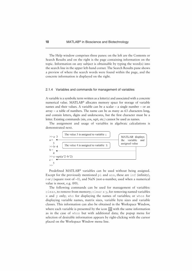
The assignment and usage of variables in algebraic calculations is demonstrated next.

Predefined MATLAB® variables can be used without being assigned. Except for the previously mentioned pi and ans, these are inf (infinity), i or j (square root of –1), and NaN (not-a-number, used when a numerical value is moot, e.g. 0/0).

The following commands can be used for management of variables: clear, to remove from memory; clear x y, for removing named variables x and y only; who for displaying the names of variables; or whos for displaying variable names, matrix sizes, variable byte sizes and variable classes. This information can also be obtained in the Workspace Window, where each variable is presented by the icon with the same information as in the case of whos but with additional data; the popup menu for selection of desirable information appears by right-clicking with the cursor placed on the Workspace Window menu line.

MATLAB® basics 11

2.1.5 Output commands

As previously noted, MATLAB® automatically displays the result after each command is entered, but does not display it if the command is followed by a semicolon. MATLAB® has additional display commands, the two most frequently used of which are disp and fprintf.

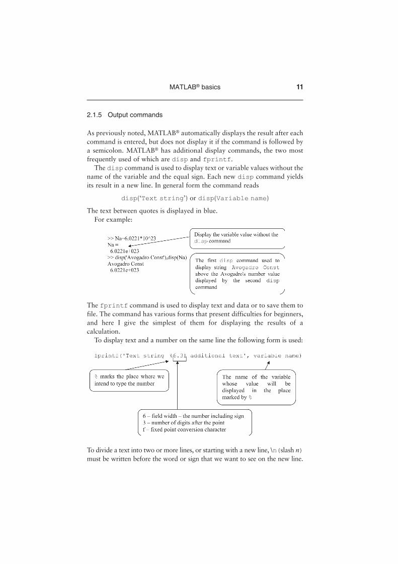
The disp command is used to display text or variable values without the name of the variable and the equal sign. Each new disp command yields its result in a new line. In general form the command reads

disp(‘Text string’) or disp(Variable name)

The text between quotes is displayed in blue.For example:

The fprintf command is used to display text and data or to save them to file. The command has various forms that present difficulties for beginners, and here I give the simplest of them for displaying the results of a calculation.

To display text and a number on the same line the following form is used:

To divide a text into two or more lines, or starting with a new line, \n(slash n) must be written before the word or sign that we want to see on the new line.

12 MATLAB® in Bioscience and Biotechnology

The field width and the number of digits after the point (6.3 in the example presented) are optional; the sign % and the character f, called conversion character, are obligatory. The character f specifies the fixed point notation in which the number is displayed. Some additional notations that can be used are: i, integer, e, exponential (e.g. 2.309123e+001); and g, the more compact form of e or f, with no trailing zeros.

Addition of several %f units (or full formatting elements) permits inclusion of multiple variable values in the text. For example, using the fprintf command:

The color of the text in quotes is the same as in disp (blue).The commands described can be used to output tables as will be shown

later, after introduction of vectors and matrices.

2.1.6 Application examples

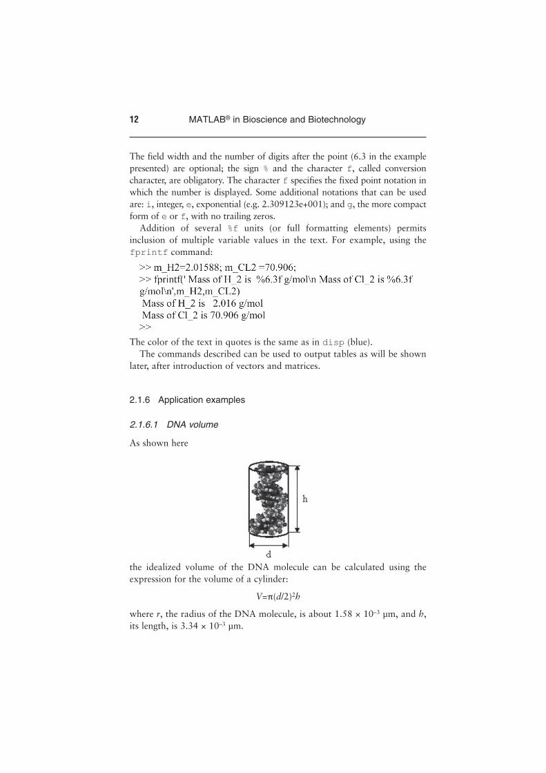
2.1.6.1 DNA volume

As shown here

the idealized volume of the DNA molecule can be calculated using the expression for the volume of a cylinder:

V=p(d/2)2h

where r, the radius of the DNA molecule, is about 1.58 × 10–3 µm, and h, its length, is 3.34 × 10–3 µm.