Embed Size (px)
Citation preview
Matlab IAn Initial Overview
Patrick O’Neil
Mathematics Testing CenterGeorge Mason University
April 1, 2016
Patrick O’Neil (GMU) Matlab I April 1, 2016 1 / 26
Introduction
Outline
1 Introduction
2 Data Structures
3 Control Flow
4 Custom Functions
5 Plotting
Patrick O’Neil (GMU) Matlab I April 1, 2016 2 / 26
Introduction
What is Matlab?
Patrick O’Neil (GMU) Matlab I April 1, 2016 3 / 26
Introduction
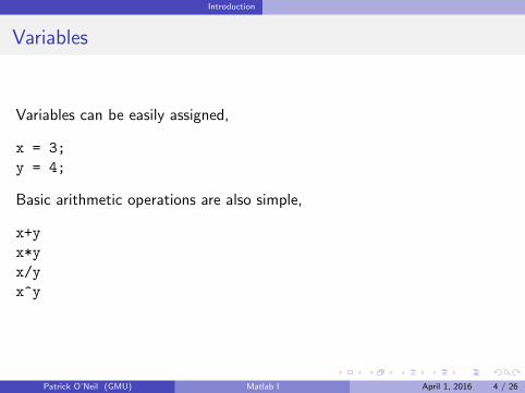
Variables
Variables can be easily assigned,
x = 3;
y = 4;
Basic arithmetic operations are also simple,
x+y
x*y
x/y
x^y
Patrick O’Neil (GMU) Matlab I April 1, 2016 4 / 26
Introduction
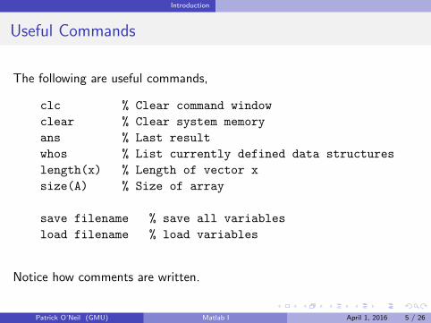
Useful Commands
The following are useful commands,
clc % Clear command window
clear % Clear system memory
ans % Last result
whos % List currently defined data structures
length(x) % Length of vector x
size(A) % Size of array
save filename % save all variables
load filename % load variables
Notice how comments are written.
Patrick O’Neil (GMU) Matlab I April 1, 2016 5 / 26
Data Structures
Outline
1 Introduction
2 Data Structures
3 Control Flow
4 Custom Functions
5 Plotting
Patrick O’Neil (GMU) Matlab I April 1, 2016 6 / 26
Data Structures
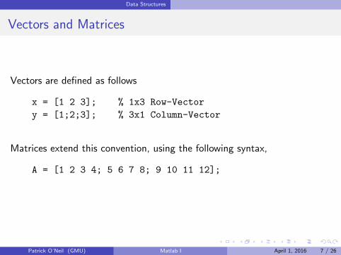
Vectors and Matrices
Vectors are defined as follows
x = [1 2 3]; % 1x3 Row-Vector
y = [1;2;3]; % 3x1 Column-Vector
Matrices extend this convention, using the following syntax,
A = [1 2 3 4; 5 6 7 8; 9 10 11 12];
Patrick O’Neil (GMU) Matlab I April 1, 2016 7 / 26
Data Structures
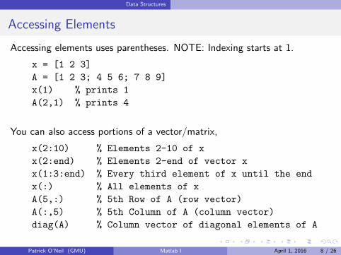
Accessing Elements
Accessing elements uses parentheses. NOTE: Indexing starts at 1.
x = [1 2 3]
A = [1 2 3; 4 5 6; 7 8 9]
x(1) % prints 1
A(2,1) % prints 4
You can also access portions of a vector/matrix,
x(2:10) % Elements 2-10 of x
x(2:end) % Elements 2-end of vector x
x(1:3:end) % Every third element of x until the end
x(:) % All elements of x
A(5,:) % 5th Row of A (row vector)
A(:,5) % 5th Column of A (column vector)
diag(A) % Column vector of diagonal elements of A
Patrick O’Neil (GMU) Matlab I April 1, 2016 8 / 26
Data Structures
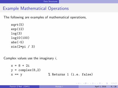
Example Mathematical Operations
The following are examples of mathematical operations,
sqrt(5)
exp(12)
log(3)
log10(100)
abs(-5)
sin(2*pi / 3)
Complex values use the imaginary i ,
x = 8 + 2i
y = complex(8,2)
x == y % Returns 1 (i.e. false)
Patrick O’Neil (GMU) Matlab I April 1, 2016 9 / 26
Data Structures
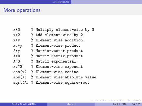
More operations
x*3 % Multiply element-wise by 3
x+2 % Add element-wise by 2
x+y % Element-wise addition
x.*y % Element-wise product
A*y % Matrix-vector product
A*B % Matrix-Matrix product
A^3 % Matrix-exponential
x.^3 % Element-wise exponent
cos(x) % Element-wise cosine
abs(A) % Element-wise absolute value
sqrt(A) % Element-wise square-root
Patrick O’Neil (GMU) Matlab I April 1, 2016 10 / 26
Data Structures
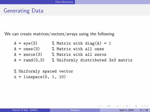
Generating Data
We can create matrices/vectors/arrays using the following
A = eye(3) % Matrix with diag(A) = 1
A = ones(3) % Matrix with all ones
A = zeros(3) % Matrix with all zeros
A = rand(3,3) % Uniformly distributed 3x3 matrix
% Uniformly spaced vector
x = linspace(0, 1, 10)
Patrick O’Neil (GMU) Matlab I April 1, 2016 11 / 26
Data Structures
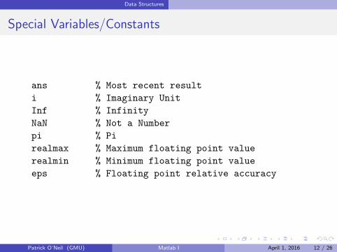
Special Variables/Constants
ans % Most recent result
i % Imaginary Unit
Inf % Infinity
NaN % Not a Number
pi % Pi
realmax % Maximum floating point value
realmin % Minimum floating point value
eps % Floating point relative accuracy
Patrick O’Neil (GMU) Matlab I April 1, 2016 12 / 26
Data Structures
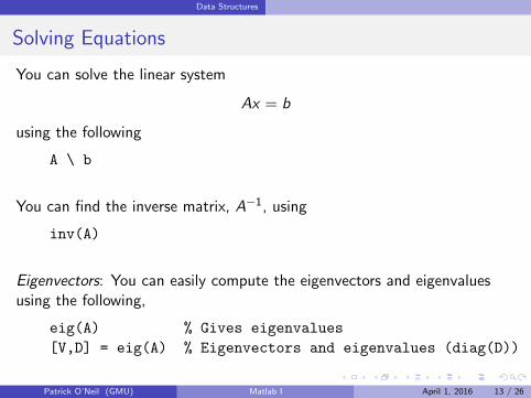
Solving Equations
You can solve the linear system
Ax = b
using the following
A \ b
You can find the inverse matrix, A−1, using
inv(A)
Eigenvectors: You can easily compute the eigenvectors and eigenvaluesusing the following,
eig(A) % Gives eigenvalues
[V,D] = eig(A) % Eigenvectors and eigenvalues (diag(D))
Patrick O’Neil (GMU) Matlab I April 1, 2016 13 / 26
Control Flow
Outline
1 Introduction
2 Data Structures
3 Control Flow
4 Custom Functions
5 Plotting
Patrick O’Neil (GMU) Matlab I April 1, 2016 14 / 26
Control Flow
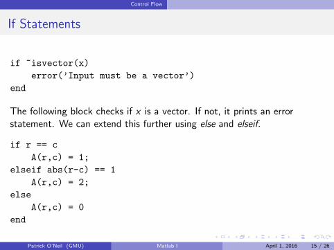
If Statements
if ~isvector(x)
error(’Input must be a vector’)
end
The following block checks if x is a vector. If not, it prints an errorstatement. We can extend this further using else and elseif.
if r == c
A(r,c) = 1;
elseif abs(r-c) == 1
A(r,c) = 2;
else
A(r,c) = 0
end
Patrick O’Neil (GMU) Matlab I April 1, 2016 15 / 26
Control Flow
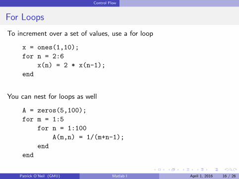
For Loops
To increment over a set of values, use a for loop
x = ones(1,10);
for n = 2:6
x(n) = 2 * x(n-1);
end
You can nest for loops as well
A = zeros(5,100);
for m = 1:5
for n = 1:100
A(m,n) = 1/(m+n-1);
end
end
Patrick O’Neil (GMU) Matlab I April 1, 2016 16 / 26
Control Flow
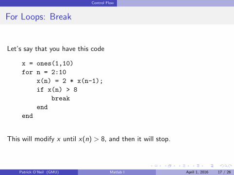
For Loops: Break
Let’s say that you have this code
x = ones(1,10)
for n = 2:10
x(n) = 2 * x(n-1);
if x(n) > 8
break
end
end
This will modify x until x(n) > 8, and then it will stop.
Patrick O’Neil (GMU) Matlab I April 1, 2016 17 / 26
Control Flow
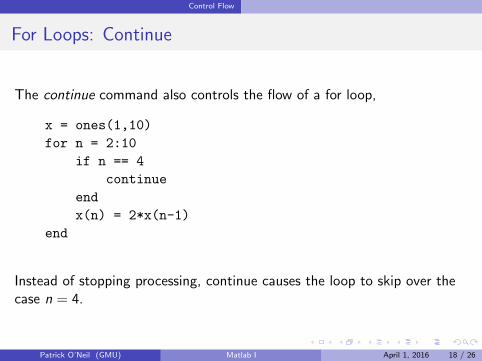
For Loops: Continue
The continue command also controls the flow of a for loop,
x = ones(1,10)
for n = 2:10
if n == 4
continue
end
x(n) = 2*x(n-1)
end
Instead of stopping processing, continue causes the loop to skip over thecase n = 4.
Patrick O’Neil (GMU) Matlab I April 1, 2016 18 / 26
Control Flow
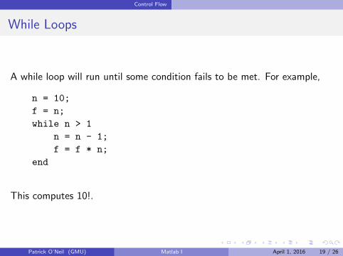
While Loops
A while loop will run until some condition fails to be met. For example,
n = 10;
f = n;
while n > 1
n = n - 1;
f = f * n;
end
This computes 10!.
Patrick O’Neil (GMU) Matlab I April 1, 2016 19 / 26
Custom Functions
Outline
1 Introduction
2 Data Structures
3 Control Flow
4 Custom Functions
5 Plotting
Patrick O’Neil (GMU) Matlab I April 1, 2016 20 / 26
Custom Functions
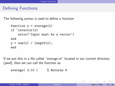
Defining Functions
The following syntax is used to define a function
function y = average(x)
if ~isvector(x)
error(’Input must be a vector’)
end
y = sum(x) / length(x);
end
If we put this in a file called “average.m” located in our current directory(pwd), then we can call the function as
average( 2:10 ) % Returns 6
Patrick O’Neil (GMU) Matlab I April 1, 2016 21 / 26
Custom Functions
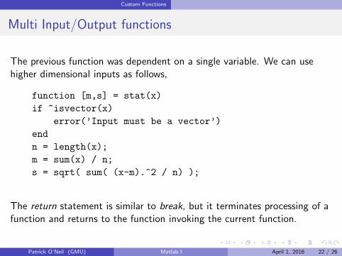
Multi Input/Output functions
The previous function was dependent on a single variable. We can usehigher dimensional inputs as follows,
function [m,s] = stat(x)
if ~isvector(x)
error(’Input must be a vector’)
end
n = length(x);
m = sum(x) / n;
s = sqrt( sum( (x-m).^2 / n) );
The return statement is similar to break, but it terminates processing of afunction and returns to the function invoking the current function.
Patrick O’Neil (GMU) Matlab I April 1, 2016 22 / 26
Plotting
Outline
1 Introduction
2 Data Structures
3 Control Flow
4 Custom Functions
5 Plotting
Patrick O’Neil (GMU) Matlab I April 1, 2016 23 / 26
Plotting
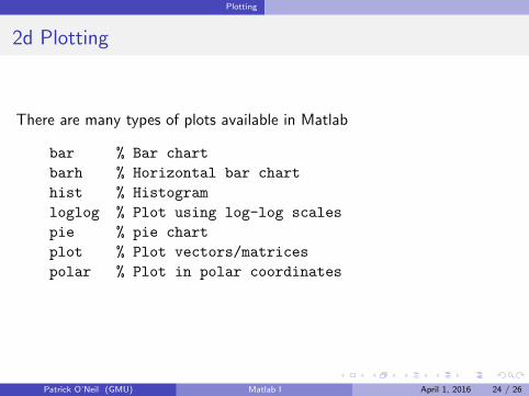
2d Plotting
There are many types of plots available in Matlab
bar % Bar chart
barh % Horizontal bar chart
hist % Histogram
loglog % Plot using log-log scales
pie % pie chart
plot % Plot vectors/matrices
polar % Plot in polar coordinates
Patrick O’Neil (GMU) Matlab I April 1, 2016 24 / 26
Plotting
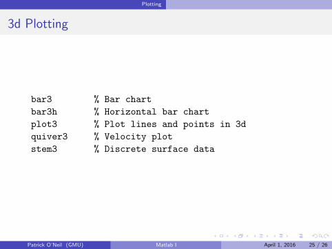
3d Plotting
bar3 % Bar chart
bar3h % Horizontal bar chart
plot3 % Plot lines and points in 3d
quiver3 % Velocity plot
stem3 % Discrete surface data
Patrick O’Neil (GMU) Matlab I April 1, 2016 25 / 26
Plotting
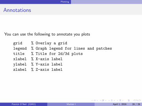
Annotations
You can use the following to annotate you plots
grid % Overlay a grid
legend % Graph legend for lines and patches
title % Title for 2d/3d plots
xlabel % X-axis label
ylabel % Y-axis label
zlabel % Z-axis label
Patrick O’Neil (GMU) Matlab I April 1, 2016 26 / 26