Embed Size (px)
Citation preview

NATIONAL INSTITUTE OF TECHNOLOGY, DURGAPUR
CE: COMPUTATIONAL LABORATORY
PROGRAMING in:
SUBMITTED by: MIAAZA HUSSAIN
10/CE/61

Programming in MATLAB
Page 2
Exercise 1: MATRIX MULTIPLICATION
Multiply two user input matrix of any size and check if the matrices can be multiplied and display the result
CODING IN M FILE clear all
clc
a=input('Matrix A = ')
b=input('Matrix B = ')
as=size(a);
bs=size(b);
% size of matrix represented (row,column)
if (as(2)==bs(1)); % here 2 represents the no of columns of matrix A
%'Matrix can be multiplied'
for i=1:as(1)
for m=1:bs(2)
sum=0;
for j=1:as(2)
sum=sum+a(i,j)*b(j,m);
end
c(i,m)=sum;
end
end
c
else
input('Matrix cannot be multiplied')
end
SOLUTION IN COMMAND WINDOW
Matrix A = [5 6 8; 8 9 0; 6 7 8]
a =
5 6 8
8 9 0
6 7 8
Matrix B = [7 8 9 0;7 6 5 8;7 7 6 8]

Programming in MATLAB
Page 3
b =
7 8 9 0
7 6 5 8
7 7 6 8
c =
133 132 123 112
119 118 117 72
147 146 137 120
Programming in MATLAB
Page 4
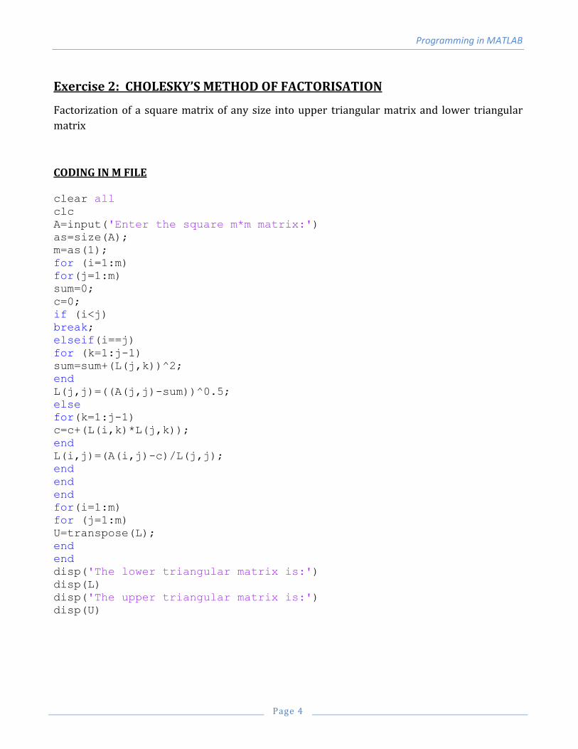
Exercise 2: CHOLESKY’S METHOD OF FACTORISATION
Factorization of a square matrix of any size into upper triangular matrix and lower triangular
matrix
CODING IN M FILE clear all clc A=input('Enter the square m*m matrix:') as=size(A); m=as(1); for (i=1:m) for(j=1:m) sum=0; c=0; if (i<j) break; elseif(i==j) for (k=1:j-1) sum=sum+(L(j,k))^2; end L(j,j)=((A(j,j)-sum))^0.5; else for(k=1:j-1) c=c+(L(i,k)*L(j,k)); end L(i,j)=(A(i,j)-c)/L(j,j); end end end for(i=1:m) for (j=1:m) U=transpose(L); end end disp('The lower triangular matrix is:') disp(L) disp('The upper triangular matrix is:') disp(U)

Programming in MATLAB
Page 5
SOLUTION IN COMMAND WINDOW
Enter the square m*m matrix:[1 3 4 6; 3 5 2 8; 4 2 9 3; 6 8 3 0]
A =
1 3 4 6
3 5 2 8
4 2 9 3
6 8 3 0
The lower triangular matrix is:
1.0000 0 0 0
3.0000 0.0000 + 2.0000i 0 0
4.0000 -0.0000 + 5.0000i 4.2426 + 0.0000i 0
6.0000 -0.0000 + 5.0000i 0.9428 + 0.0000i 0.0000 + 3.4480i
The upper triangular matrix is:
1.0000 3.0000 4.0000 6.0000
0 0.0000 + 2.0000i -0.0000 + 5.0000i -0.0000 + 5.0000i
0 0 4.2426 + 0.0000i 0.9428 + 0.0000i
0 0 0 0.0000 + 3.4480i

Programming in MATLAB
Page 6
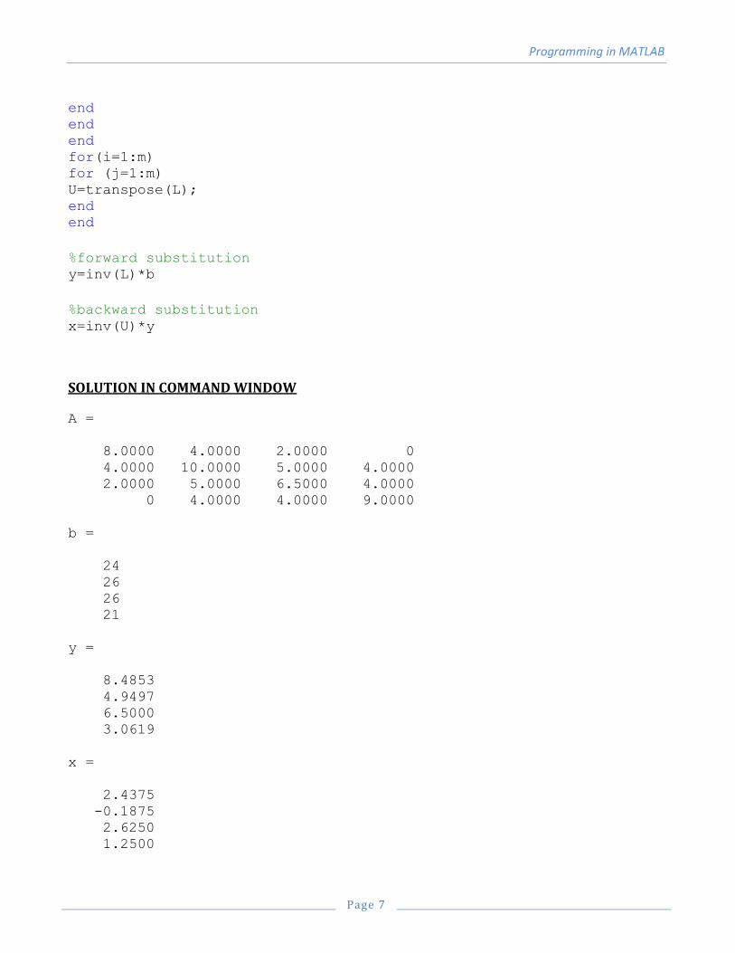
Exercise 3: USING CHOLESKY DEPOSITION TO SOLVE SET OF LINEAR EQUATIONS (FORWARD AND BACKWARD SUBSTITUTION)
Solve the following set of equations: 8z+4y+2j+0K=24,
4z+10y+5j+4k=26,
2z+5y+6.5j+4k=26,
0z+4y+4j+9k=21,
CODING IN M FILE % A=[8 4 2 0;4 10 5 4;2 5 6.5 4;0 4 4 9] % x=[z;y;j;k] % b=[24;26;26;21] %Ax=b %LUx=B %forward substitution: solve for y-----> Ly=b----> y=inv(L)b %backward substitution: solve for x-----> y=Ux------> x=inv(U)
clear all clc A=[8 4 2 0;4 10 5 4;2 5 6.5 4;0 4 4 9] b=[24;26;26;21] as=size(A); m=as(1);
%choleski factorization for (i=1:m) for(j=1:m) sum=0; c=0; if (i<j) break; elseif(i==j) for (k=1:j-1) sum=sum+(L(j,k))^2; end L(j,j)=((A(j,j)-sum))^0.5; else for(k=1:j-1) c=c+(L(i,k)*L(j,k)); end L(i,j)=(A(i,j)-c)/L(j,j);
Programming in MATLAB
Page 7
end end end for(i=1:m) for (j=1:m) U=transpose(L); end end
%forward substitution y=inv(L)*b
%backward substitution x=inv(U)*y
SOLUTION IN COMMAND WINDOW
A =
8.0000 4.0000 2.0000 0
4.0000 10.0000 5.0000 4.0000
2.0000 5.0000 6.5000 4.0000
0 4.0000 4.0000 9.0000
b =
24
26
26
21
y =
8.4853
4.9497
6.5000
3.0619
x =
2.4375
-0.1875
2.6250
1.2500

Programming in MATLAB
Page 8
Exercise 4: STODOLAS METHOD for MODAL ANALYSIS OF BUILDING FRAMES
Example problem:
Five-story shear plane frame with story-height of 3.0m and single bay of 4.0m • The mathematical model consists from squares columns ( 60× 60cm2 ) with infinitely rigid beams ( = ∞ beam I ). • The entire mass of each story is assumed to be lumped at its level with total value of typical story mass (m = 100kN.sec2/ m). • The material of columns and beams has modulus of elasticity equal to ( E = 2.106 kN /m2 ). • Assumed damping ratio (ζ = 0.05). • The frame is subjected to dynamic response spectra as defined in UBC-97 with assumed design parameters : ♦ Seismic zone factor ( Z = 0.3) ♦ Soil profile type ( B S ) CODING IN M FILE
clear all clc M=[100 0 0 0 0; 0 100 0 0 0; 0 0 100 0 0; 0 0 0 100 0; 0 0 0 0 100]; %kc=2*12EIc E=2*10^6; I=0.0108; %in m^4 h=3; k1=(2*12*E*I)/(h^3); k2=k1;k3=k1;k4=k1;k5=k1; K=[k1 -k1 0 0 0;-k1 k1+k2 -k2 0 0;0 -k2 k2+k3 -k3 0; 0 0 -k3 k3+k4 -
k4; 0 0 0 -k4 k4+k5];
%mode shapes and omega [modeshape,omega]=eig(inv(M)*K)
%determination of frequancy matrix freq=zeros(5);
for i=1:5 freq(i,i)=omega(i,i)^0.5; end

Programming in MATLAB
Page 9
freq %in rad/sec
% plotting 1st mode shape for i=1:5 for j=1 modeshape1(i,j)=modeshape(i,1); end end y=15:-h:3; x=modeshape1; plot(x,y,'b-') xlabel('Displacement') ylabel('Height') Axis([-0.1,1,0,16]) title('MODAL ANALYSIS(10/CE/61)')
SOLUTION IN COMMAND WINDOW modeshape =
0.5969 0.5485 0.4557 -0.3260 0.1699
0.5485 0.1699 -0.3260 0.5969 -0.4557
0.4557 -0.3260 -0.5485 -0.1699 0.5969
0.3260 -0.5969 0.1699 -0.4557 -0.5485
0.1699 -0.4557 0.5969 0.5485 0.3260
omega =
15.5547 0 0 0 0
0 132.5335 0 0 0
0 0 329.3511 0 0
0 0 0 543.5194 0
0 0 0 0 707.0414
freq =
3.9439 0 0 0 0
0 11.5123 0 0 0
0 0 18.1480 0 0
0 0 0 23.3135 0
0 0 0 0 26.5902

Programming in MATLAB
Page 10
Fig: 1st mode shape

Programming in MATLAB
Page 11
Exercise 5: SECOND ORDER DIFFERENTIAL EQUATION BY APPLYING NEWTON RAPHSON METHOD
Example problem: Spring mass damper system: Plot the response of a forced system given
by the equation
m ẍ+ c ẋ+ kx =f sinωt
For ξ = 0.1; m = 1 kg; k = 100 N/m; F = 100 N; ω = 2ωn; x(0) = 2 m;0
Natural frequency ωn =√ = 10 rad/sec
c/m=2ξωn; c=2
For ξ = 0.1;
Damped natural frequency ωd = ωn √ ξ = 9.95 rad/sec.
Damped time period Td = 2π/ωd = 0.63 sec. (Therefore, for five time cycles the
interval should be 5 times the damped time period, i.e., 3.16sec. Since the plots should
indicate both the transient and the steady state response, the time interval will be
increased)
CODING IN M FILE function myode clc clear all [t,x]=ode45(@func,[0 5],[0.02 0]); plot(t,x(:,1),'m-'); xlabel('time'); ylabel('Displacement'); title('ODE45 by Miaaza Hussain, 10/CE/61') function rk=func(t,x) mass=1; omega=9.95; c=2; F=100; k=100; rk=[x(2);(F/mass*sin(omega*t))-(k*x(1)/mass)-(c*x(2)/mass)]; end

Programming in MATLAB
Page 12
SOLUTION IN COMMAND WINDOW