Embed Size (px)
Citation preview

Maths for Finance
Fundamentals of Probability
Paul SchneiderFinance Group
Warwick Business [email protected]
September, 2011
P.Schneider - Warwick Business School

Fundamentals of Probability
Outline
1. Sample space and events2. Probability and random variables3. Probability density functions4. Cumulative distribution function5. Quantile and quantile function6. Joint probability density functions7. Marginal probability density functions8. Independence9. Expected value, variance, covariance, correlation
10. Conditional expectation, conditional variance11. Skewness and kurtosis12. References
P.Schneider - Warwick Business School 1

Sample space and events
Sample space is the collection of all possible outcomes that can result from a randomexperiment
Examples:
1. Traded volume of “FTSE100” index:sample space is the set of non-negative integer numbers= N+
0
2. Log-returns on closing prices of “FTSE100” index:sample space is the set of real numbers = R
3. Default within one year of the firm “Marks & Spencer”:sample space is {Default, non-Default}
Date Close Volume
15/09/08 5204.2 208749140012/09/08 5416.7 137529470011/09/08 5318.4 144887790010/09/08 5366.2 158067730009/09/08 5415.6 200876420008/09/08 5446.3 80805650005/09/08 5240.7 165344910004/09/08 5362.1 142420680003/09/08 5499.7 125768260002/09/08 5620.7 1347035700
Source:
http://finance.yahoo.com
P.Schneider - Warwick Business School 2

Sample space and events
An event is a subset of the sample space
Examples:
1. Event: Traded volume of “FTSE100” index is largerthan 2× 10⁹
2. Event: The negative Log-returns on closing pricesof “FTSE100” index
3. Event: The firm “Marks & Spencer” defaults withinone year
Date Close Log‐ return Volume
15/09/08 5204.2 ‐0.01738 208749140012/09/08 5416.7 0.00795 137529470011/09/08 5318.4 ‐0.00389 144887790010/09/08 5366.2 ‐0.00398 158067730009/09/08 5415.6 ‐0.00245 200876420008/09/08 5446.3 0.01671 80805650005/09/08 5240.7 ‐0.00995 165344910004/09/08 5362.1 ‐0.01100 142420680003/09/08 5499.7 ‐0.00945 125768260002/09/08 5620.7 0.00139 1347035700
5602.8Source: http://finance.yahoo.com
P.Schneider - Warwick Business School 3

Sample space and events
An elementary event is a subset of the sample space with only one element
Examples: which of the following are elementary events?
1. Event: Traded volume of “FTSE100” index isequal to 808, 056, 500
2. Event: The positive Log-returns on closing pricesof “FTSE100” index
3. Event: Closing Price of “FTSE100” index is equalto 5, 000.0
4. Event: The firm “Marks & Spencer” defaults withinone year
Date Close Log‐ return Volume
15/09/08 5204.2 ‐0.01738 208749140012/09/08 5416.7 0.00795 137529470011/09/08 5318.4 ‐0.00389 144887790010/09/08 5366.2 ‐0.00398 158067730009/09/08 5415.6 ‐0.00245 200876420008/09/08 5446.3 0.01671 80805650005/09/08 5240.7 ‐0.00995 165344910004/09/08 5362.1 ‐0.01100 142420680003/09/08 5499.7 ‐0.00945 125768260002/09/08 5620.7 0.00139 1347035700
5602.8Source: http://finance.yahoo.com
P.Schneider - Warwick Business School 4

Sample space and events
Several events are mutually exclusive if they have no outcomes in common
Examples: which of the following events are mutually exclusive?
1. Event A: The positive Log-returns on closing pricesof “FTSE100” index
Event B: The negative Log-returns on closingprices of “FTSE100” index
2. Event A: The firm “Marks & Spencer” defaultswithin one year
Event B: The firm “Marks & Spencer” defaults ordoes not default within one year
Date Close Log‐ return Volume
15/09/08 5204.2 ‐0.01738 208749140012/09/08 5416.7 0.00795 137529470011/09/08 5318.4 ‐0.00389 144887790010/09/08 5366.2 ‐0.00398 158067730009/09/08 5415.6 ‐0.00245 200876420008/09/08 5446.3 0.01671 80805650005/09/08 5240.7 ‐0.00995 165344910004/09/08 5362.1 ‐0.01100 142420680003/09/08 5499.7 ‐0.00945 125768260002/09/08 5620.7 0.00139 1347035700
5602.8Source: http://finance.yahoo.com
P.Schneider - Warwick Business School 5

Sample space and events
A set of events is said to be exhaustive if it contains all the elements of the samplespace
Examples: which of the following sets of events are exhaustive?
1. Event A: The positive Log-returns on closing pricesof “FTSE100” index
Event B: The negative Log-returns on closingprices of “FTSE100” index
2. Event A: The firm “Marks & Spencer” defaultswithin one year
Event B: The firm “Marks & Spencer” defaults ordoes not default within one year
Date Close Log‐ return Volume
15/09/08 5204.2 ‐0.01738 208749140012/09/08 5416.7 0.00795 137529470011/09/08 5318.4 ‐0.00389 144887790010/09/08 5366.2 ‐0.00398 158067730009/09/08 5415.6 ‐0.00245 200876420008/09/08 5446.3 0.01671 80805650005/09/08 5240.7 ‐0.00995 165344910004/09/08 5362.1 ‐0.01100 142420680003/09/08 5499.7 ‐0.00945 125768260002/09/08 5620.7 0.00139 1347035700
5602.8Source: http://finance.yahoo.com
P.Schneider - Warwick Business School 6

Probability and random variables
The probability of an event A, denoted P (A), is the chance that A occurs
Examples: 1. Event A: The Log-returns on closing prices of “FTSE100” index arepositive: P (A) = 52%
2. Event A: “Credit Suisse” defaults within one year1: P (A) = 0.008%
Source: http://www.credit-suisse.com - 16/09/08
For calibration of default probabilities to ratings see Bluhm, Overbeck & Wagner (2003) An Introduction to Credit Risk
Modeling
P.Schneider - Warwick Business School 7

Probability and random variables
P (A) is a function on the set of all possible events with the following properties:
1. 0 ≤ P (A) ≤ 1 for every event A
2. If A,B,C, . . . is an exhaustive set of events, then P (A+B + C + . . .) = 1Example:
P (“Credit Suisse” defaults or does not default) = 1
3. If A,B,C, . . . are mutually exclusive events, then
P (A+B + C + . . .) = P (A) + P (B) + P (C) + . . .
Example:
P (The Log-returns on FTSE are positive or are negative) =
= P (Log-returns on FTSE are positive) + P (Log-returns on FTSE are negative)
P.Schneider - Warwick Business School 8

Random variables
A random variable, rv, is a variable taking values given by a chance experiment
Examples:
• rv S representing the future closing price of “FTSE100” index
• rv X representing the future Log-return on closing prices of “FTSE100” index
• rv V representing the future traded volume of “FTSE100” index
• rv L representing default or non-default within one year of “Credit Suisse (Bank)”
P.Schneider - Warwick Business School 9

Random variables
A discrete random variable can only assume a countable number of values
A continuous random variable can assume any value in an interval
Examples: which of the following rvs are continuous and which ones are discrete?
• rv S representing the closing price of “FTSE100” index
• rv X representing the Log-return on closing prices of “FTSE100” index
• rv V representing the traded volume of “FTSE100” index
• rv L representing default or non-default within one year of “Credit Suisse (Bank)”
P.Schneider - Warwick Business School 10

Probability density functions (pdf)
Discrete random variables
If L is a discrete rv taking values l1, l2, l3, . . ., then the function
f(l) = P (L = li) for i = 1, 2, 3, . . .
= 0 for l 6= li
is the (discrete) probability density function (pdf) of L
Example:
rv L representing default or non-default within one year of “Credit Suisse (Bank)”
L takes values 1 if default occurs and 0 if default does not occur
f(1) = P (L = 1) = 0.008%
f(0) = P (L = 0) = 1− 0.008% = 99.992%
P.Schneider - Warwick Business School 11

Probability density functions (pdf)
Continuous random variables
If X is a continuous rv, then f(x) is the pdf of X iif
f(x) ≥ 0∫ +∞
−∞f(x)dx = 1
In this case the probability of X ∈ [a, b] is P (a ≤ X ≤ b) =∫ baf(x)dx
Example:rv X representing the Log-return on “FTSE100”
P (X > 0) =∫ +∞0
f(x)dx = 52%
P (X = a) =∫ aaf(x)dx = 0
Probability density function
P.Schneider - Warwick Business School 12

Cumulative distribution function (cdf)
Continuous random variables
If X is a continuous rv, then its cdf for any realnumber is
F (x) = P (X ≤ x)
• Because F (x) is a probability, 0 ≤ F (x) ≤ 1
• If a ≤ b then F (a) ≤ F (b)
• If a ≤ b then P (a ≤ X ≤ b) = F (b)− F (a)
• For any c, P (X > c) = 1− P (X ≤ c) Probability density function
• For a continuous rv and any real number a, P (X = a) = 0 then
P (X < a) = P (X ≤ a)
P.Schneider - Warwick Business School 13

Quantile and quantile function, qα
If X is a rv, then the quantile of probability α is the real number, denoted qα, whichleaves the probability α to its left:
P (X ≤ qα) = F (qα) = α
Whenever the cdf F has inverse the quantile function is
F−1(α) = qα ⇐⇒ α = F (qα)
In the general case
qα = min{x : F (x) ≥ α}
Example: Value-at-Risk is a quantile
X represents the log-returns on FTSE
α = 0.99
q0.99 = F−1(0.99) is the 99% Value-at-Risk (VaR99%)
P.Schneider - Warwick Business School 14

Joint probability density function
The joint probability density function of two discrete variables X and Y is
f(x, y) = P (X = x and Y = y)
= 0 when X 6= x and Y 6= y
Example:
L1 represents default or non-default of “Credit Suisse”
L2 represents default or non-default of “Marks and Spencer”
L2\L1 0 10 0.980 0.001 0.9811 0.003 0.016 0.019
0.983 0.017 1
Note: Probabilities of default are exaggerated
P.Schneider - Warwick Business School 15

Joint probability density function
The function f(x, y) is the joint probability density function of the continuous rvsX and Y iif
f(x, y) ≥ 0 and
∫ +∞
−∞
∫ +∞
−∞f(x, y)dxdy = 1
In this case P (a ≤ X ≤ b, c ≤ Y ≤ d) =∫ dc
∫ baf(x, y)dxdy
Example:
• X1 represents the log-returns of “FTSE100”
• X2 represents the log-returns of “S&P500”
The probability that both “FTSE100” and “S&P500” have a large loss of 15% or moreis
P (X1 ≤ −0.15, X2 ≤ −0.15) =
∫ −0.15−∞
∫ −0.15−∞
f(x1, x2)dx1dx2
P.Schneider - Warwick Business School 16

Marginal probability density function
Given a probability density function f(x, y), the marginal probability density functionsof X and Y are:
f(x) =∑y
f(x, y)
f(y) =∑x
f(x, y)
Example: From the previous example
L2\L1 0 1 f(l2)0 0.980 0.001 0.9811 0.003 0.016 0.019
f(l1) 0.983 0.017 1
if X and Y are discrete rvs, and
f(x) =
∫ +∞
−∞f(x, y)dy
f(y) =
∫ +∞
−∞f(x, y)dx
if X and Y are continuous rvs
P.Schneider - Warwick Business School 17

Independence
Two random variables X and Y (discrete or continuous) are independent, iif
f(x, y) = f(x)f(y)
Example: In which case are the default of the two firms independent?
L2\L1 0 1 f(l2)0 0.980 0.001 0.9811 0.003 0.016 0.019
f(l1) 0.983 0.017 1
L2\L1 0 1 f(l2)0 0.9643 0.0167 0.9811 0.0187 0.0003 0.019
f(l1) 0.983 0.017 1
P.Schneider - Warwick Business School 18

Expected value
The expected value of a discrete rv X, denoted E(X), is defined as
E(X) =∑x
xf(x)
The expected value of a continuous rv X, denoted E(X), is defined as
E(X) =
∫ +∞
−∞xf(x)dx
Examples: • rv L represents default or non-default of “Credit Suisse”:
E(L) = 0× 0.99992 + 1× 0.00008 = 0.00008
• rv L represents default of an obligor and e = 106 is the exposure. Theexpected value of a loss from this obligor is
E(eL) = 0× 0.99992 + 106 × 0.00008 = 80
P.Schneider - Warwick Business School 19

Properties of the expected value
1. E(a) = a, for any constant a
• e = 106 is the exposure of an obligor.
The expected value of the exposure is: E(e) = E(106) = 106
2. E(aX + b) = aE(X) + b for any constants a and b and rv X
• rv L represents default of an obligor and e = 106 is the exposure.
The expected value of a loss from this obligor (assuming recovery equal to zero) is:
E(eL) = e× E(L) = 106 × 0.00008 = 80
3. If X and Y are independent rvs then, E(XY ) = E(X)E(Y )
• If the rv loss-given-default (LGD) of an obligor is independent of its creditrating (default: L) then the expected value of a loss is:
E(e× LGD × L) = e× E(LGD)× E(L) = 106 × 0.4× 0.00008 = 32
P.Schneider - Warwick Business School 20

Properties of the expected value (cont)
4. If the rv X has pdf f(x) and g(X) is any function of X, then
E[g(X)] =∑x
g(x)f(x) if X is discrete
=
∫ +∞
−∞g(x)f(x)dx if X is continuous
Example:
• rv X representing the log-returns on FTSE100. If
g(x) = |x|
then the expected value of the absolute log-returns is∫ +∞
−∞|x|f(x)dx
P.Schneider - Warwick Business School 21
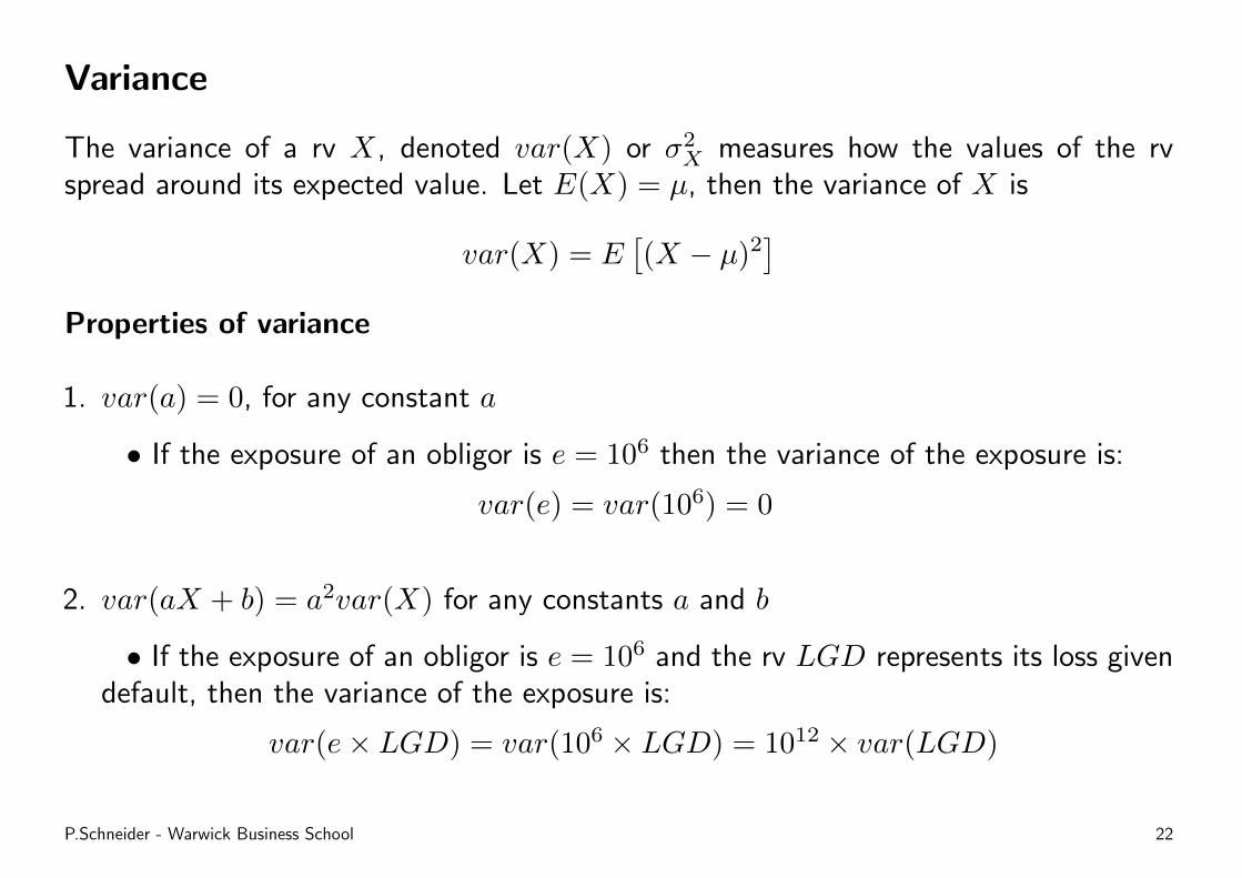
Variance
The variance of a rv X, denoted var(X) or σ2X measures how the values of the rv
spread around its expected value. Let E(X) = µ, then the variance of X is
var(X) = E[(X − µ)2
]Properties of variance
1. var(a) = 0, for any constant a
• If the exposure of an obligor is e = 106 then the variance of the exposure is:
var(e) = var(106) = 0
2. var(aX + b) = a2var(X) for any constants a and b
• If the exposure of an obligor is e = 106 and the rv LGD represents its loss givendefault, then the variance of the exposure is:
var(e× LGD) = var(106 × LGD) = 1012 × var(LGD)
P.Schneider - Warwick Business School 22

Properties of variance (cont)
3. If X and Y are independent rvs, then
var(X + Y ) = var(X) + var(Y ) and var(X − Y ) = var(X) + var(Y )
• rv X1 representing the losses on FTSE100• rv X2 representing the losses on S&P500
If the losses on FTSE100 and S&P500 are independent then the var of the lossesof a portfolio composed of both indices is:
var(X1 +X2) = var(X1) + var(X2)
4. var(X) = E(X2)− (E(X))2
The standard deviation, σX, is the positive square root of the variance of X
P.Schneider - Warwick Business School 23

Covariance
If X and Y are two rvs with means µX and µY , then the covariance between X and Yis
cov(X,Y ) = E [(X − µx)(Y − µY )] = E(XY )− µXµY
Properties of covariance
1. If X and Y are independent then cov(X,Y ) = 0 (but not vice-versa!!)2. cov(a+ bX, c+ dY ) = bd cov(X,Y )
Variance-covariance matrix• rv X representing the log-returns on FTSE100• rv Y representing the log-returns on S&P500
The variance-covariance matrix is
V arCov =
[var(X) cov(X,Y )
cov(Y,X) var(Y )
]=
[0.3 0.06
0.06 0.4
]
P.Schneider - Warwick Business School 24
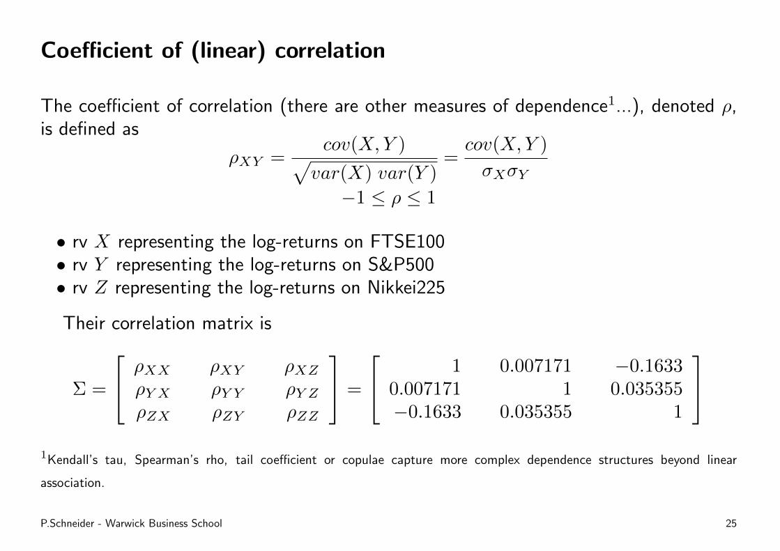
Coefficient of (linear) correlation
The coefficient of correlation (there are other measures of dependence1...), denoted ρ,is defined as
ρXY =cov(X,Y )√var(X) var(Y )
=cov(X,Y )
σXσY
−1 ≤ ρ ≤ 1
• rv X representing the log-returns on FTSE100• rv Y representing the log-returns on S&P500• rv Z representing the log-returns on Nikkei225
Their correlation matrix is
Σ =
ρXX ρXY ρXZρY X ρY Y ρY ZρZX ρZY ρZZ
=
1 0.007171 −0.16330.007171 1 0.035355−0.1633 0.035355 1
1Kendall’s tau, Spearman’s rho, tail coefficient or copulae capture more complex dependence structures beyond linear
association.
P.Schneider - Warwick Business School 25

Variance of correlated variables
If X and Y are two rvs, then
var(X ± Y ) = var(X) + var(Y )± 2 cov(X,Y )
In general, for n rvs X1, X2, . . . , Xn,
var
(n∑i=1
Xi
)=
n∑i=1
var(Xi) + 2∑∑
i<jcov(Xi, Xj)
Example: From the previous example
V arCov =
0.3 0.006 −0.040.006 0.4 0.01−0.04 0.01 0.2
The var of a portfolio composed of the three indices is:
var(X + Y + Z) = 0.3 + 0.4 + 0.2 + 2× (0.006− 0.04 + 0.01) = 0.852
P.Schneider - Warwick Business School 26

Conditional expectation
If f(x, y) is the joint pdf of the rvs X and Y , then the conditional expectation of X,given that Y = y, denoted E(X|Y = y) or µX|Y , is
E(X|Y = y) =∑x
xf(x|Y = y) if X is discrete
=
∫ +∞
−∞xf(x|Y = y)dx if X is continuous
where f(x|Y = y) is the pdf of X|Y which is given by f(x|Y = y) = f(x, y)/f(y)
Example:
• The expected shortfall or conditional VaR is a conditional expectationrv X represents the log-returns on FTSE then the 99% expected shortfall is
ES99% = E(X|X > VaR99%)
P.Schneider - Warwick Business School 27
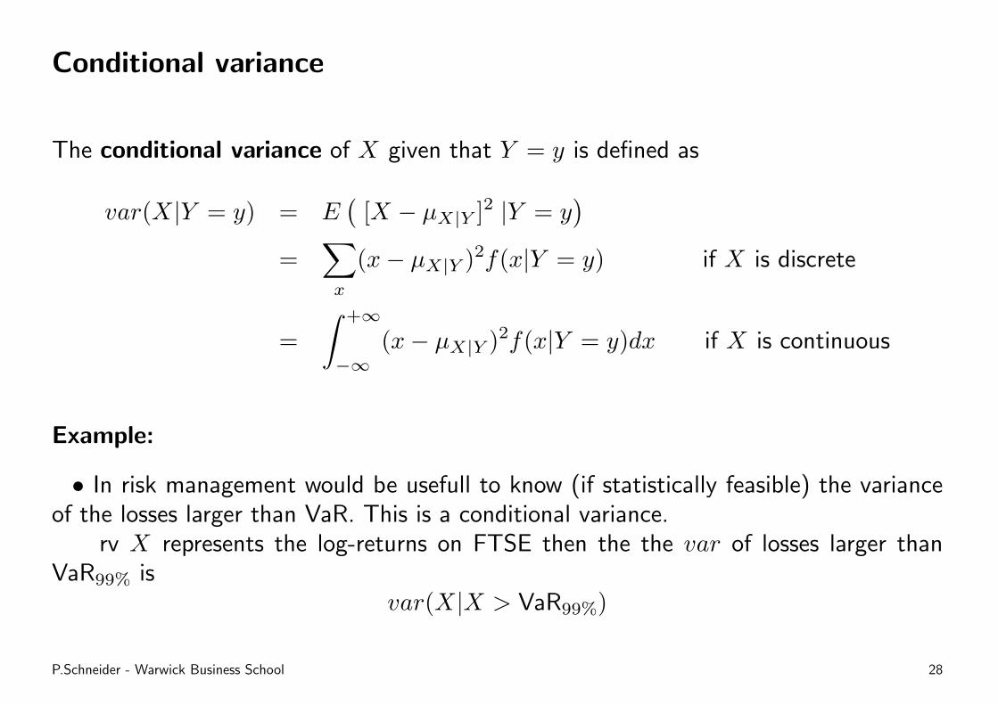
Conditional variance
The conditional variance of X given that Y = y is defined as
var(X|Y = y) = E(
[X − µX|Y ]2 |Y = y)
=∑x
(x− µX|Y )2f(x|Y = y) if X is discrete
=
∫ +∞
−∞(x− µX|Y )2f(x|Y = y)dx if X is continuous
Example:
• In risk management would be usefull to know (if statistically feasible) the varianceof the losses larger than VaR. This is a conditional variance.
rv X represents the log-returns on FTSE then the the var of losses larger thanVaR99% is
var(X|X > VaR99%)
P.Schneider - Warwick Business School 28

Properties of conditional expectation and conditional variance
1. If f(X) is a function of X, then E(f(X)|X) = f(X)
2. If f(X) and g(X) are functions of X, then
E(f(X)Y + g(X)|X) = f(X)E(Y |X) + g(X)
3. If X and Y are independent, E(X|Y ) = E(X)
4. E(Y ) = E(E(Y |X))
5. If X and Y are independent, var(X|Y ) = var(X)
6. var(Y ) = E(var(Y |X)) + var(E(Y |X))
P.Schneider - Warwick Business School 29

Skewness
In general the rth moment about the mean is defined as
E[(X − µ)r]
The coefficient of skewness is a measure of asymmetry of a pdf and is defined basedon the third moment as
E[(X − µ)3]
σ3
Example: Daily (high-frequency) log-returns on financial assets often reveal a negativeskewness (towards the losses tail!) =⇒ large losses are more frequent than large gains!
P.Schneider - Warwick Business School 30

Kurtosis
The coefficient of kurtosis is a measure of flatness of a pdf and is defined based onthe forth moment as
E[(X − µ)4]
σ4
Example: High kurtosis is synonymous of heavy tails! Higher probability of occurrenceof extreme values (losses)! Large impact in VaR, economic capital. Very important inrisk management, pricing, hedging!
P.Schneider - Warwick Business School 31

References
The topics covered in this section and more on probability can be found in more detail,for instance, in one of the following references:
• Kmenta, J. (1997), Elements of Econometrics, 2nd Edition, University of MichiganPress. Chapter 3
• Maddala, G.S. (2001), Introduction to Econometrics, 3rd Edition, Wiley. Chapter 2
• Mittelhamer, Ron C. (1996), Mathematical Statistics for Economics and Business,Springer-Verlag New York Inc. Chapters 1–5
• Newbold, P., Carlson, W.L. and Thorne, B. (2003) Statistics for Business andEconomics, 5th Edition, Prentice Hall. Chapters 4–6
P.Schneider - Warwick Business School 32