1 23

Journal of Mathematical Chemistry ISSN 0259-9791 J Math ChemDOI 10.1007/s10910-014-0322-4

Estimation of rate constants in nonlinearreactions involving chemical inactivation ofoxidation catalysts

Maria Emelianenko, Diego Torrejon,Matthew A. DeNardo, AnnikaK. Socolofsky, Alexander D. Ryabov &Terrence J. Collins

1 23

Your article is protected by copyright and

all rights are held exclusively by Springer

International Publishing Switzerland. This e-

offprint is for personal use only and shall not

be self-archived in electronic repositories. If

you wish to self-archive your article, please

use the accepted manuscript version for

posting on your own website. You may

further deposit the accepted manuscript

version in any repository, provided it is only

made publicly available 12 months after

official publication or later and provided

acknowledgement is given to the original

source of publication and a link is inserted

to the published article on Springer's

website. The link must be accompanied by

the following text: "The final publication is

available at link.springer.com”.

J Math ChemDOI 10.1007/s10910-014-0322-4

ORIGINAL PAPER

Estimation of rate constants in nonlinear reactionsinvolving chemical inactivation of oxidation catalysts

Maria Emelianenko · Diego Torrejon ·Matthew A. DeNardo · Annika K. Socolofsky ·Alexander D. Ryabov · Terrence J. Collins

Received: 20 November 2013 / Accepted: 28 January 2014© Springer International Publishing Switzerland 2014

Abstract Over the last decades, copious work has been devoted to the developmentof small molecule replicas of the peroxidase enzymes that activate hydrogen peroxidein metabolic and detoxifying processes. TAML activators that are the subject of thisstudy are the first full functional, small molecule peroxidase mimics. As an impor-tant feature of the catalytic cycle, TAML reactive intermediates (active catalysts, Ac)undergo suicidal inactivation, compromising the functional catalysis. Herein the rela-tionship between suicidal inactivation and productive catalysis is rigorously addressedmathematically and chemically. We focus on a generalized catalytic cycle in whichthe TAML inactivation step is delineated by its rate constant ki where the revealingdata is collected in the regime of incomplete conversion of substrate (S) artificiallyimposed by the use of very low catalyst concentrations.

⎧⎨

⎩

Resting catalyst (Rc) + Oxidant → Ac (kI)

Ac + Substrate (S) → Rc + Product (kII)

Ac → Inactive catalyst (ki)

The system exhibits a nonlinear conservation law and is modeled via a singular per-turbation approach, which is used to obtain closed form relationships between systemparameters. A new method is derived that allows to compute all the rate constants inthe catalytic cycle, kI, kII, and ki, with as little as two linear least squares fits, for the

M. Emelianenko (B) · D. TorrejonDepartment of Mathematical Sciences, George Mason University,4400 University Dr, Fairfax, VA 22030, USAe-mail: memelian@gmu.edu

M. A. DeNardo · A. K. Socolofsky · A. D. Ryabov (B) · T. J. CollinsDepartment of Chemistry, Carnegie Mellon University,4400 Fifth Ave, Pittsburgh, PA 15213, USAe-mail: ryabov@andrew.cmu.edu

123

Author's personal copy

J Math Chem

minimal data set collected under any conditions providing that the oxidation of S isincomplete. This method facilitates determination of ki, a critical rate constant thatdescribes the operational lifetime of the catalyst, and greatly reduces the experimentalwork required to obtain the important rate constants.The approach was applied to thebehavior of a new TAML activator, the synthesis and characterization of which arealso described.

Keywords Iron TAMLs · Hydrogen peroxide · Catalyst inactivation ·Ordinary differential equations · Mathematical modeling · Perturbation methods

1 Introduction

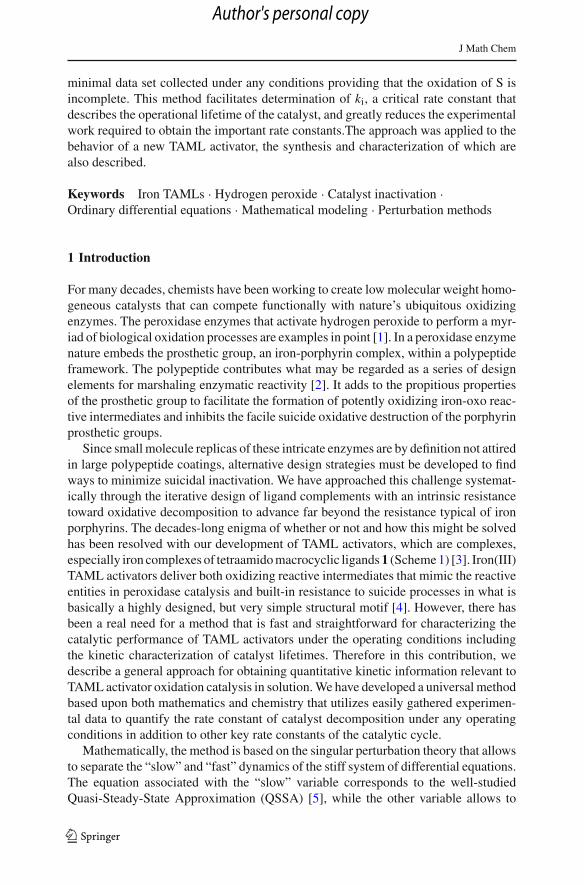
For many decades, chemists have been working to create low molecular weight homo-geneous catalysts that can compete functionally with nature’s ubiquitous oxidizingenzymes. The peroxidase enzymes that activate hydrogen peroxide to perform a myr-iad of biological oxidation processes are examples in point [1]. In a peroxidase enzymenature embeds the prosthetic group, an iron-porphyrin complex, within a polypeptideframework. The polypeptide contributes what may be regarded as a series of designelements for marshaling enzymatic reactivity [2]. It adds to the propitious propertiesof the prosthetic group to facilitate the formation of potently oxidizing iron-oxo reac-tive intermediates and inhibits the facile suicide oxidative destruction of the porphyrinprosthetic groups.

Since small molecule replicas of these intricate enzymes are by definition not attiredin large polypeptide coatings, alternative design strategies must be developed to findways to minimize suicidal inactivation. We have approached this challenge systemat-ically through the iterative design of ligand complements with an intrinsic resistancetoward oxidative decomposition to advance far beyond the resistance typical of ironporphyrins. The decades-long enigma of whether or not and how this might be solvedhas been resolved with our development of TAML activators, which are complexes,especially iron complexes of tetraamido macrocyclic ligands 1 (Scheme 1) [3]. Iron(III)TAML activators deliver both oxidizing reactive intermediates that mimic the reactiveentities in peroxidase catalysis and built-in resistance to suicide processes in what isbasically a highly designed, but very simple structural motif [4]. However, there hasbeen a real need for a method that is fast and straightforward for characterizing thecatalytic performance of TAML activators under the operating conditions includingthe kinetic characterization of catalyst lifetimes. Therefore in this contribution, wedescribe a general approach for obtaining quantitative kinetic information relevant toTAML activator oxidation catalysis in solution. We have developed a universal methodbased upon both mathematics and chemistry that utilizes easily gathered experimen-tal data to quantify the rate constant of catalyst decomposition under any operatingconditions in addition to other key rate constants of the catalytic cycle.

Mathematically, the method is based on the singular perturbation theory that allowsto separate the “slow” and “fast” dynamics of the stiff system of differential equations.The equation associated with the “slow” variable corresponds to the well-studiedQuasi-Steady-State Approximation (QSSA) [5], while the other variable allows to

123

Author's personal copy

J Math Chem

Scheme 1 First (1) and second (2) generations of Fe-TAML activators. Axial Y ligand is usually water orchloride. Catalyst 2 with X1 = CN and Orange II dye were used in this work

capture the rapid evolution of the system in the boundary layer. This approach hasbeen applied to chemical kinetics problems by several authors [6,7], although noneof the previous work has addressed the inherently nonlinear chemical inactivationproblem. The main contribution of the present work is the derivation of a generalmechanism for estimating rate constants based on the closed form representation ofthe solution obtained via the singular perturbation method. The method allows to obtainthe full set of rate constants associated with the nonlinear kinetic model of chemicalinactivation using only two linear least square fitting procedures. This approach isdrastically different from the multiple variable optimization method sometimes called“kinetic modeling”, which feeds a solution obtained by a full-blown stiff solver into amulti-parameter least squares optimization routine [8,9]. Given the nonlinear nature ofthe chemical inactivation problem described above, such a procedure would be costly,while yielding multiple plausible solution vectors indistinguishable from the point ofview of the goodness of fit. In what follows, we develop a simple-to-use strategy thatis devoid of these deficiencies while having a solid mathematical foundation.

2 Background and motivation

2.1 Background

Although TAML activators are potent oxidation catalysts, multiple degradationprocesses are known to bear directly on the catalytic performance in water(Scheme 2) [10]. A particular advantage of the method elaborated herein is that itprovides a simple tool for evaluating the rate constant of the dominating degradationstep. For catalyst design purposes, it is important to be able to rank the destruc-tive capacity of each identified process by finding the intrinsic rate constants underoperating conditions. Several decomposition pathways open up simply when TAMLactivators are dissolved in water. Thus, in the absence of an oxidizing agent the rest-ing catalyst (Rc) decays due to demetalation (kd) [11,12]. Still others come into playwhen hydrogen peroxide (H2O2) is added [13]. Upon peroxide addition, the Rc reactsreversibly (kI, k−I) with H2O2 to form the active catalyst (Ac), which then may attackthe targeted substrate S in a product-producing reaction quantified by kII. The intrinsicrate constants of the resting state demetalations are known to be immensely smallerthan those associated with kI and kII, such that the former are of negligible significanceunder operating catalysis, but once the Ac has been formed, suicidal decomposition

123

Author's personal copy

J Math Chem

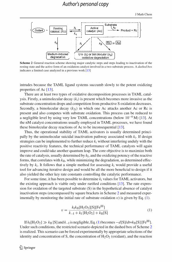
Scheme 2 General reaction scheme showing major catalytic steps and steps leading to inactivation of theresting state and the active form of an oxidation catalyst involved in a two-substrate process. A dashed boxindicates a limited case analyzed in a previous work [13]

intrudes because the TAML ligand systems succumb slowly to the potent oxidizingproperties of Ac [13].

There are at least two types of oxidative decomposition processes in TAML catal-ysis. Firstly, a unimolecular decay (ki) is present which becomes more invasive as thesubstrate concentration drops and competition from productive S oxidation decreases.Secondly, a bimolecular decay (k2i) in which one Ac attacks another Ac or Rc ispresent and also competes with substrate oxidation. This process can be reduced toa negligible level by using very low TAML concentrations (below 10−6 M) [13]. Atthe nM catalyst concentrations usually employed in TAML processes, we have foundthese bimolecular decay reactions of Ac to be inconsequential [13].

Thus, the operational stability of TAML activators is usually determined princi-pally by the unimolecular suicidal inactivation pathway associated with ki. If designstrategies can be implemented to further reduce ki without interfering unduly with thepositive reactivity features, the technical performance of TAML catalysts will againimprove and could take another quantum leap. The core objective is to maximize boththe rate of catalysis, usually determined by kI, and the oxidizing potency of the reactiveforms, that correlates with kII, while minimizing the degradation, as determined effec-tively by ki. It follows that a simple method for assessing ki would provide a usefultool for advancing iterative design and would be all the more beneficial to design if italso yielded the other key rate constants controlling the catalytic performance.

For some time, it has been possible to determine ki values for TAML activators, butthe existing approach is viable only under rarified conditions [13]. The rate expres-sion for oxidation of the targeted substrate (S) in the hypothetical absence of catalystinactivation steps (encompassed by square brackets in Scheme 2 and measured exper-imentally by monitoring the initial rate of substrate oxidation v) is given by Eq. (1).

v = kIkII[H2O2][S][FeIII]k−I + kI [H2O2] + kII[S] (1)

If kI[H2O2] � kII [S] and k−I is negligible, Eq. (1) becomes−d[S]/dt=kII[S] [FeIII].Under such conditions, the restricted scenario depicted in the dashed box of Scheme 2is realized. This scenario can be forced experimentally by appropriate selections of theidentity and concentration of S, the concentration of H2O2 (oxidant), and the reaction

123

Author's personal copy

J Math Chem

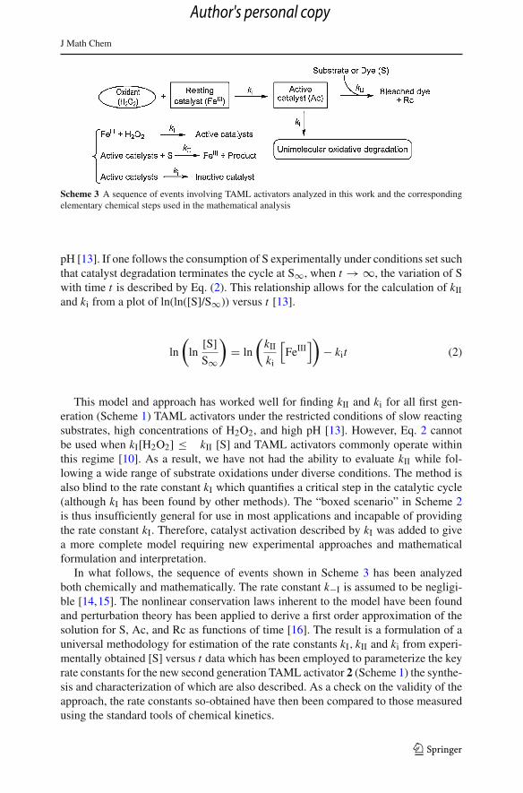
Scheme 3 A sequence of events involving TAML activators analyzed in this work and the correspondingelementary chemical steps used in the mathematical analysis

pH [13]. If one follows the consumption of S experimentally under conditions set suchthat catalyst degradation terminates the cycle at S∞, when t → ∞, the variation of Swith time t is described by Eq. (2). This relationship allows for the calculation of kIIand ki from a plot of ln(ln([S]/S∞)) versus t [13].

ln

(

ln[S]

S∞

)

= ln

(kII

ki

[FeIII

])

− kit (2)

This model and approach has worked well for finding kII and ki for all first gen-eration (Scheme 1) TAML activators under the restricted conditions of slow reactingsubstrates, high concentrations of H2O2, and high pH [13]. However, Eq. 2 cannotbe used when kI[H2O2] ≤ kII [S] and TAML activators commonly operate withinthis regime [10]. As a result, we have not had the ability to evaluate kII while fol-lowing a wide range of substrate oxidations under diverse conditions. The method isalso blind to the rate constant kI which quantifies a critical step in the catalytic cycle(although kI has been found by other methods). The “boxed scenario” in Scheme 2is thus insufficiently general for use in most applications and incapable of providingthe rate constant kI. Therefore, catalyst activation described by kI was added to givea more complete model requiring new experimental approaches and mathematicalformulation and interpretation.

In what follows, the sequence of events shown in Scheme 3 has been analyzedboth chemically and mathematically. The rate constant k−I is assumed to be negligi-ble [14,15]. The nonlinear conservation laws inherent to the model have been foundand perturbation theory has been applied to derive a first order approximation of thesolution for S, Ac, and Rc as functions of time [16]. The result is a formulation of auniversal methodology for estimation of the rate constants kI, kII and ki from experi-mentally obtained [S] versus t data which has been employed to parameterize the keyrate constants for the new second generation TAML activator 2 (Scheme 1) the synthe-sis and characterization of which are also described. As a check on the validity of theapproach, the rate constants so-obtained have then been compared to those measuredusing the standard tools of chemical kinetics.

123

Author's personal copy

J Math Chem

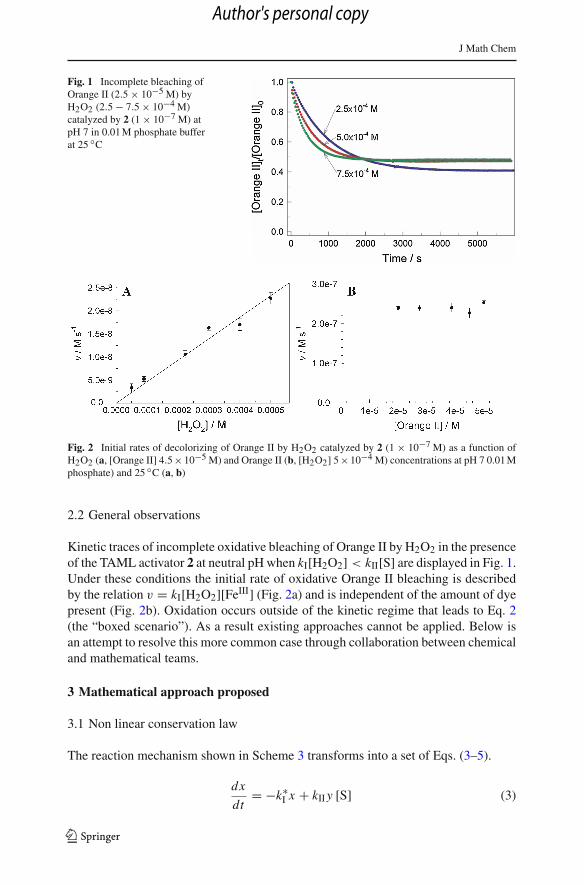
Fig. 1 Incomplete bleaching ofOrange II (2.5 × 10−5 M) byH2O2 (2.5 − 7.5 × 10−4 M)catalyzed by 2 (1 × 10−7 M) atpH 7 in 0.01 M phosphate bufferat 25 ◦C

Fig. 2 Initial rates of decolorizing of Orange II by H2O2 catalyzed by 2 (1 × 10−7 M) as a function ofH2O2 (a, [Orange II] 4.5 × 10−5 M) and Orange II (b, [H2O2] 5 × 10−4 M) concentrations at pH 7 0.01 Mphosphate) and 25 ◦C (a, b)

2.2 General observations

Kinetic traces of incomplete oxidative bleaching of Orange II by H2O2 in the presenceof the TAML activator 2 at neutral pH when kI[H2O2] < kII[S] are displayed in Fig. 1.Under these conditions the initial rate of oxidative Orange II bleaching is describedby the relation v = kI[H2O2][FeIII] (Fig. 2a) and is independent of the amount of dyepresent (Fig. 2b). Oxidation occurs outside of the kinetic regime that leads to Eq. 2(the “boxed scenario”). As a result existing approaches cannot be applied. Below isan attempt to resolve this more common case through collaboration between chemicaland mathematical teams.

3 Mathematical approach proposed

3.1 Non linear conservation law

The reaction mechanism shown in Scheme 3 transforms into a set of Eqs. (3–5).

dx

dt= −k∗

I x + kII y [S] (3)

123

Author's personal copy

J Math Chem

dy

dt= k∗

I x − kII y [S] − ki y (4)

d [S]

dt= −kII y [S] (5)

Here x, y, and [S] are the current concentrations of the Rc [FeIII], Ac, and the OrangeII dye, respectively, and k∗

I = kI[H2O2] as the concentration of H2O2 is assumed tobe constant because [H2O2] � [S] such that its consumption can be neglected. Byusing UV-vis spectroscopy, the concentration of Orange II can be easily and accuratelymeasured as a function of time for bleaching curves measured at different peroxideconcentrations and therefore it is an observable parameter. The system satisfies thefollowing boundary conditions: x(0) = x0, y(0) = 0, [S]0 = S0 and x∞ = 0, y∞ =0, [S]∞ = S∞ because all forms of the catalyst eventually vanish. Simple algebraicoperations lead to a nonlinear conservation law, of which Eq. (6) is the differentialform.

d

dt

(

x + y − ki

kIIln [S]

)

= 0 (6)

Integration of Eq. (6) taking into account the initial conditions affords Eq. (7).

x = ki

kIIln

([S]

S0

)

− y + x0 (7)

Equation (7) allows one to reduce the dimensions of the problem, gives a nonlinearconservation law for this system that can be employed to estimate the rate constants,and as t → ∞ it becomes Eq. (8).

lnS0

S∞= kII

kix0 (8)

If R = ln(

S0S∞

)Eq. (8) becomes Eq. (9).

kII = R

x0ki (9)

This conclusion is identical to that previously reached for the “boxed scenario” inScheme 1, i.e. when kI[H2O2] < kII[S] [9]. Here we have shown that this importantrelation holds regardless of the relative values of kI[H2O2] and kII[S].

3.2 Perturbation solution

Nondimensional concentrations will further be used as y = x0 y, x = x0 x, and[S] = S0[S] because the initial concentrations of all the participants are known. Anappropriate time scaling is then provided by t = tcτ with tc = 1/x0kII. Using theconservation law [Eq. (7)] together with the scaling laws, the system of Eqs. (3–5)simplifies to:

123

Author's personal copy

J Math Chem

d[S]

dτ= −y

[S]

(10)

εd y

dτ= β ln

[S] − y

([S] + α

) + ζ (11)

where

β = k∗I ki

k2IIS0x0

, α = k∗I + ki

kIIS0, ζ = k∗

I

kIIS0, ε = x0

S0(12)

The experimental conditions used in this study imply that ε is ca. 10−3. This sug-gests that a boundary layer exists which separates fast and slow dynamics in the model.Thus, it is appropriate to apply the tools of perturbation theory to this situation [5,16].The perturbation argument leading to approximate solutions for changes of S concen-trations with time both inside and outside the boundary layer of width ε can be derived,which can then be assembled into a composite solution through a matching procedure.Outside the boundary layer (in the outer region), regular asymptotic expansions withrespect to ε in the form of y = y0 + ε y1 . . . and [S] = S0 + ε S1 . . . have been usedfor the Ac and the substrate, respectively. A first order approximation then leads to:

d S0

dτ= −yS0 (13)

0 = β lnS0 − y0(S0 + α

) + ζ (14)

This system can be interpreted as a quasi-state approximation commonly used inkinetic modeling [6,17]. In order to derive an analytical solution, an approximationof the form S0 + α ∼ A(α+1) is introduced, with A being a constant independent ofkI, kII, and ki. This approximation holds for the outer layer, where S0 changes onlyslightly. This allows one to obtain the following representation for the substrate changein the outer region:

S0 = e− ζβ e

Cβe

(− β

a(α+1)τ)

(15)

Here C is an integration constant to be determined. Note that ζ / β = R, so Eq. (15)can be further simplified as:

S0 = S∞S0

eCβ

e

(− β

a(α +1)τ)

(16)

By plugging (16) into (14), one obtains the corresponding representation of the Acbehavior in the outer region:

Y = y0 = C

A(α+1)e

(− β

a(α+1)tct)

(17)

These are the explicit outer region solutions for the concentrations of the Ac [Eq. (17)]and of the substrate [(S)] [Eq. (16)]. The outer solution is denoted by Y to distinguish itfrom the inner solution. Note that S0 → S∞/S0 and y0 → 0 as τ → ∞, as expected.

123

Author's personal copy

J Math Chem

To approximate the solution in the inner region, a singular perturbation expansion tozoom into the boundary layer was performed. If τ is scaled by τ = τ ε, the first orderapproximation generates:

d S0

d τ= 0 (18)

d y0

d τ= β lnS0 − y0

(α+S0

) + ζ (19)

which implies[S] = S0 = 1 (20)

y = y0 = ζ

α +1

(1 − e− (α +1)

tcεt)

(21)

These inner solutions for [S] and the Ac are denoted as [S] and y, respectively. Tomatch the values of y and Y at the boundary layer, the following condition should beimposed:

limt→0

Y = limt→∞ y

This is necessary because the outer solution must match the inner solution as timeapproaches zero. In the same fashion, the inner solution must match the outer solutionas time approaches infinity. By applying the previous condition to the Ac and S, onecan see that this condition is equivalent to: R = AR, C = ζ. We conclude that A = 1and set the value of the integration constant to C = ζ. After matching the two piecesof the solution, the following composite solution is obtained:

y

x0= ζ

α+1

(

e− β

(α +1)tct − e

−(α+1)εtc

t)

(22)

[S]

S0= S∞

S0eRe

− β(α+1)tc

t

(23)

Equations (22)–(23) are the final closed form asymptotic solutions for the Ac and Swhich will be used hereafter. The concentration of S as in Eq. (23) satisfies Eq. (24).

ln

(

ln[S]

S∞

)

= lnR − M1t (24)

where

M1 = β

(α+1) tc(25)

Equation (24) is the unrestricted analogue of Eq. (2). A double logarithmic plot of[S]/S∞ versus time t should be a linear function of time with the intercept and slopeof lnR and −M1, respectively (M1 > 0). Expanding the expression for M1 usingEq. (12), one gets:

123

Author's personal copy

J Math Chem

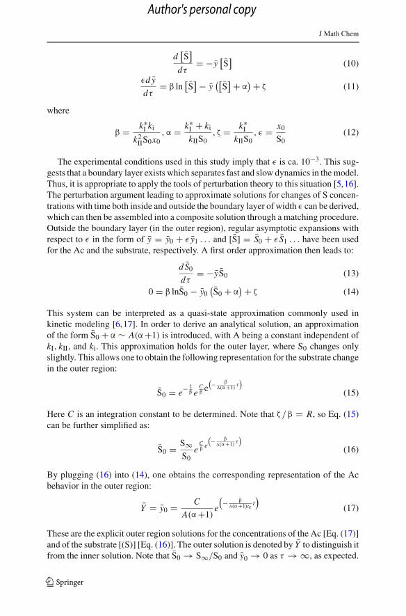
Fig. 3 Linear least squares fitting of the experimental data in Fig. 1 to Eq. (24)

M1 = kI [H2O2] ki

kI [H2O2] + ki + kIIS0(26)

It is worth noting that when t → ∞, Eq. (24) agrees with the definition R =ln(S0/S∞), and Eq. (26) converts to ki when kI[H2O2] � ki + kII[S] which agreeswith the earlier approach [13]. Results of a linear least squares fitting of the experi-mental data for three different concentrations of H2O2 are shown in Fig. 3. A goodstraight-line approximation is observed for 5–10 half-lives. Small deviations observedat the highest H2O2 concentrations are negligible due to the fact that no bleachingactually occurs after 2,000 s.

3.3 Estimation of the rate constants

The solution given by Eq. (23) was applied to solve the inverse problem, i.e. to estimatethe rate constants kI, kII and ki from the experimental data given in Fig. 1. The slopes ofthe straight lines in Fig. 3 obtained using Equation (24) depend on H2O2 concentration.From Eqs. (9) and (26) it comes

ki = M1x0k∗I

x0k∗I − x0 M1 − M1S0 R

(27)

Here M1 denotes the slope obtained from the fit, and R is the same constant asappears in Eq. (9). Equation (26) can be presented as

1

M1= 1

ki+ M2

1

[H2O2](28)

M2 = ki + kIIS0

kIki(29)

123

Author's personal copy

J Math Chem

[H2O2]-1 / M-1

0 1000 2000 3000 4000

(Slo

pe M

1)-1

/ s

0

200

400

600

800

1000

1200

1400

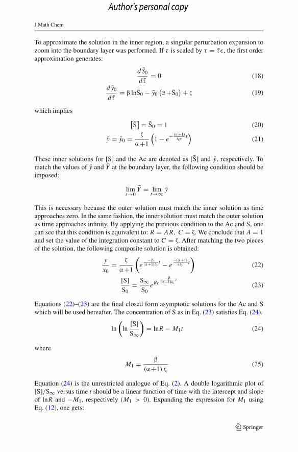
Fig. 4 Double reciprocal plot of the slopes M1 versus peroxide concentrations. The linear fit results in aslope of M2 = 0.3123

The inverse of the slopes M1 vary linearly with inverse peroxide concentrations[Eq. (28)] and the slope and the intercept equal M2 and k−1

i , respectively (Fig. 4).Finally, combining Eqs. (9) and (29) gives the expression for the rate constant kI.

kI = x0 + S0 R

x0 M2(30)

Combination of Eqs. (30) and (27) gives the expression for ki.

ki = M1 [H2O2]

[H2O2] − M1 M2(31)

Equations (9), (30), and (31) are the key equations for computing the rate constants.A routine has been developed for the determination of kI, kII, and ki.

Mathematical algorithm (MA) for estimating the rate constants:

GIVEN: [S] versus t data measured at several different [H2O2] with the same [S]0 andx0 as shown in Fig. 1.PROCEDURE:

1. For each [H2O2] data set, one computes the corresponding value of R = ln(S0/S∞)

using the best approximation of S∞ available.2. For each [H2O2] data set, one fits the data to Eq. (24) to get M1.3. Using M1 obtained in Step 2, one fits M−1

1 versus [H2O2]−1 to Eq. (28) to get M2.4. One calculates kI from Eq. (30) for each data set.5. One calculates ki from Eq. (31) for each data set.6. One uses ki obtained in Step 5 to calculate kII using Equation (9) for each data set.

The rate constants kI, kII, and ki can be calculated from kinetic data such as areshown in Fig. 1 for the oxidation of any substrate by any peroxide provided the kinetic

123

Author's personal copy

J Math Chem

data are collected at different concentrations of peroxide. Estimating M2 by the slopeis rather accurate even for a small number of data points (experimental data sets) dueto the inherently linear nature of the dependence of M−1

1 on [H2O2]−1, while theaccuracy of M−1

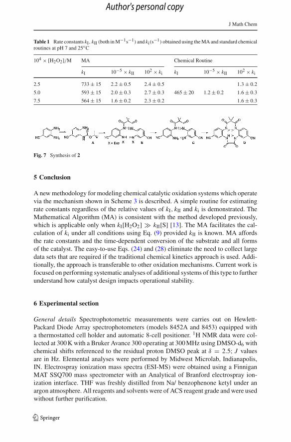
1 estimation is reliant upon the quality of experimental observationsfor 5–10 half-lives in each of the data sets. The rate constants calculated by the MAfor the new dicyano-substituted iron(III)-containing TAML activator 2 are shown inTable 1.

The new method provides explicit equations for the current concentrations of Ac,Rc, and substrate as a function of time without a priori knowledge of the rate constants.In fact, Eqs. (3–5) afford

[S] = S∞eRe−M1t(32)

y = x0 ζ

α+1

(e−M1t − e−(k∗

I +ki+kIIS0)t)

(33)

x = x0

Rln

([S]

S0

)

− y + x0 (34)

where

R = ζ

β, M1 = β

(α+1) tc, tc = 1

x0kII, β = k∗

I ki

k2IIS0x0

, α = k∗I + ki

kIIS0, ζ = k∗

I

kIIS0(35)

and the accuracy is on the order of ε, where

ε = x0

S0(36)

4 Verification of the new mathematical algorithm (MA)

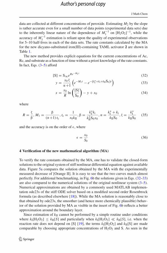
To verify the rate constants obtained by the MA, one has to validate the closed-formsolutions to the original system of stiff nonlinear differential equation against availabledata. Figure 5a compares the solution obtained by the MA with the experimentallymeasured decrease of [Orange II]. It is easy to see that the two curves match almostperfectly. For additional benchmarking, in Fig. 6b the solutions given in Eqs. (32–33)are also compared to the numerical solutions of the original nonlinear system (3–5).Numerical approximations are obtained by a commonly used MATLAB implemen-tation ode23s of the stiff ODE solver based on a modified second order Rosenbrockformula (as described elsewhere [18]). While the MA solution is reasonably close tothat obtained by ode23s, the smoother (and hence more chemically plausible) behav-ior of the solution provided by MA as visible in the insert of Fig. 6b reflects a betterapproximation around the boundary layer.

Since estimation of kII cannot be performed by a simple routine under conditionswhere kI[H2O2] ≤ kII[S] and particularly when kI[H2O2] kII[S], i.e. when thereaction rate does not depend on [S] [19], the terms kI[H2O2] and kII[S] are madecomparable by choosing appropriate concentrations of H2O2 and S. As seen in the

123

Author's personal copy

J Math Chem

Fig. 5 Comparison of the new approximation (32,33) with experimentally measured Orange II data col-lected at [H2O2] = 2.5 × 10−4, [Orange II]0 = 2.5 × 10−5 in 0.01 M phosphate buffer at pH 7 and thesolutions obtained by the ode23s stiff ODE solver

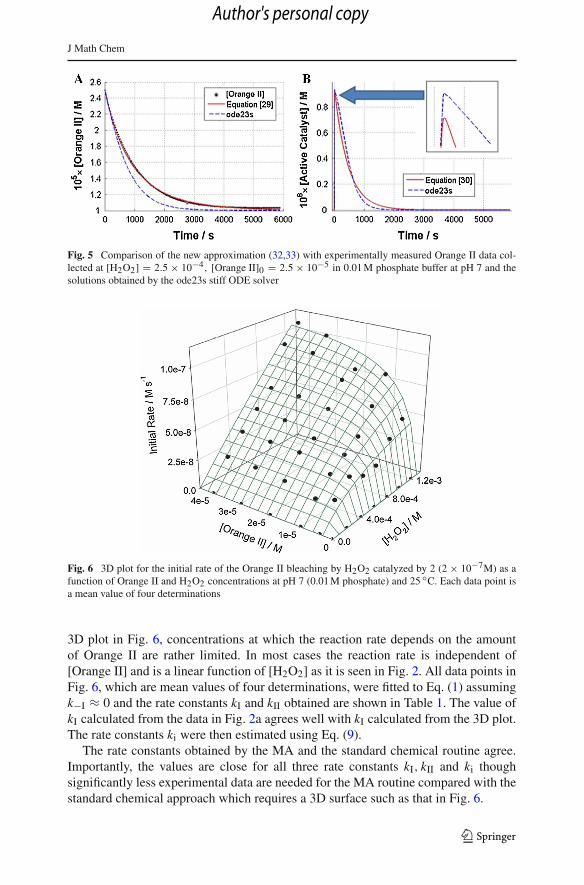
Fig. 6 3D plot for the initial rate of the Orange II bleaching by H2O2 catalyzed by 2 (2 × 10−7M) as afunction of Orange II and H2O2 concentrations at pH 7 (0.01 M phosphate) and 25 ◦C. Each data point isa mean value of four determinations

3D plot in Fig. 6, concentrations at which the reaction rate depends on the amountof Orange II are rather limited. In most cases the reaction rate is independent of[Orange II] and is a linear function of [H2O2] as it is seen in Fig. 2. All data points inFig. 6, which are mean values of four determinations, were fitted to Eq. (1) assumingk−I ≈ 0 and the rate constants kI and kII obtained are shown in Table 1. The value ofkI calculated from the data in Fig. 2a agrees well with kI calculated from the 3D plot.The rate constants ki were then estimated using Eq. (9).

The rate constants obtained by the MA and the standard chemical routine agree.Importantly, the values are close for all three rate constants kI, kII and ki thoughsignificantly less experimental data are needed for the MA routine compared with thestandard chemical approach which requires a 3D surface such as that in Fig. 6.

123

Author's personal copy

J Math Chem

Table 1 Rate constants kI, kII (both in M−1s−1) and ki(s−1) obtained using the MA and standard chemicalroutines at pH 7 and 25◦C

104 × [H2O2]/M MA Chemical Routine

kI 10−5 × kII 102 × ki kI 10−5 × kII 102 × ki

2.5 733 ± 15 2.2 ± 0.5 2.4 ± 0.5 1.3 ± 0.2

5.0 593 ± 15 2.0 ± 0.3 2.7 ± 0.3 465 ± 20 1.2 ± 0.2 1.6 ± 0.3

7.5 564 ± 15 1.6 ± 0.2 2.3 ± 0.2 1.6 ± 0.3

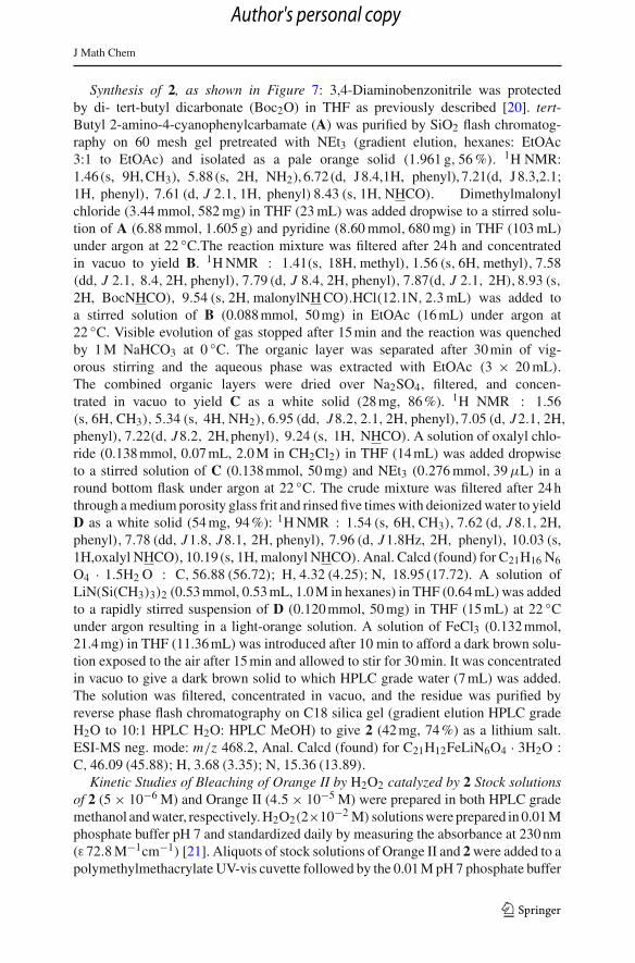
Fig. 7 Synthesis of 2

5 Conclusion

A new methodology for modeling chemical catalytic oxidation systems which operatevia the mechanism shown in Scheme 3 is described. A simple routine for estimatingrate constants regardless of the relative values of kI, kII and ki is demonstrated. TheMathematical Algorithm (MA) is consistent with the method developed previously,which is applicable only when kI[H2O2] � kII[S] [13]. The MA facilitates the cal-culation of ki under all conditions using Eq. (9) provided kII is known. MA affordsthe rate constants and the time-dependent conversion of the substrate and all formsof the catalyst. The easy-to-use Eqs. (24) and (28) eliminate the need to collect largedata sets that are required if the traditional chemical kinetics approach is used. Addi-tionally, the approach is transferable to other oxidation mechanisms. Current work isfocused on performing systematic analyses of additional systems of this type to furtherunderstand how catalyst design impacts operational stability.

6 Experimental section

General details Spectrophotometric measurements were carries out on Hewlett-Packard Diode Array spectrophotometers (models 8452A and 8453) equipped witha thermostatted cell holder and automatic 8-cell positioner. 1H NMR data were col-lected at 300 K with a Bruker Avance 300 operating at 300 MHz using DMSO-d6 withchemical shifts referenced to the residual proton DMSO peak at δ = 2.5; J valuesare in Hz. Elemental analyses were performed by Midwest Microlab, Indianapolis,IN. Electrospray ionization mass spectra (ESI-MS) were obtained using a FinniganMAT SSQ700 mass spectrometer with an Analytical of Branford electrospray ion-ization interface. THF was freshly distilled from Na/ benzophenone ketyl under anargon atmosphere. All reagents and solvents were of ACS reagent grade and were usedwithout further purification.

123

Author's personal copy

J Math Chem

Synthesis of 2, as shown in Figure 7: 3,4-Diaminobenzonitrile was protectedby di- tert-butyl dicarbonate (Boc2O) in THF as previously described [20]. tert-Butyl 2-amino-4-cyanophenylcarbamate (A) was purified by SiO2 flash chromatog-raphy on 60 mesh gel pretreated with NEt3 (gradient elution, hexanes: EtOAc3:1 to EtOAc) and isolated as a pale orange solid (1.961 g, 56 %). 1H NMR:1.46 (s, 9H, CH3), 5.88 (s, 2H, NH2), 6.72 (d, J 8.4,1H, phenyl), 7.21(d, J 8.3,2.1;1H, phenyl), 7.61 (d, J 2.1, 1H, phenyl) 8.43 (s, 1H, NHCO). Dimethylmalonylchloride (3.44 mmol, 582 mg) in THF (23 mL) was added dropwise to a stirred solu-tion of A (6.88 mmol, 1.605 g) and pyridine (8.60 mmol, 680 mg) in THF (103 mL)under argon at 22 ◦C.The reaction mixture was filtered after 24 h and concentratedin vacuo to yield B. 1H NMR : 1.41(s, 18H, methyl), 1.56 (s, 6H, methyl), 7.58(dd, J 2.1, 8.4, 2H, phenyl), 7.79 (d, J 8.4, 2H, phenyl), 7.87(d, J 2.1, 2H), 8.93 (s,2H, BocNHCO), 9.54 (s, 2H, malonylNH CO).HCl(12.1N, 2.3 mL) was added toa stirred solution of B (0.088 mmol, 50 mg) in EtOAc (16 mL) under argon at22 ◦C. Visible evolution of gas stopped after 15 min and the reaction was quenchedby 1 M NaHCO3 at 0 ◦C. The organic layer was separated after 30 min of vig-orous stirring and the aqueous phase was extracted with EtOAc (3 × 20 mL).The combined organic layers were dried over Na2SO4, filtered, and concen-trated in vacuo to yield C as a white solid (28 mg, 86 %). 1H NMR : 1.56(s, 6H, CH3), 5.34 (s, 4H, NH2), 6.95 (dd, J8.2, 2.1, 2H, phenyl), 7.05 (d, J2.1, 2H,

phenyl), 7.22(d, J8.2, 2H, phenyl), 9.24 (s, 1H, NHCO). A solution of oxalyl chlo-ride (0.138 mmol, 0.07 mL, 2.0 M in CH2Cl2) in THF (14 mL) was added dropwiseto a stirred solution of C (0.138 mmol, 50 mg) and NEt3 (0.276 mmol, 39 μL) in around bottom flask under argon at 22 ◦C. The crude mixture was filtered after 24 hthrough a medium porosity glass frit and rinsed five times with deionized water to yieldD as a white solid (54 mg, 94 %): 1H NMR : 1.54 (s, 6H, CH3), 7.62 (d, J8.1, 2H,phenyl), 7.78 (dd, J1.8, J8.1, 2H, phenyl), 7.96 (d, J1.8Hz, 2H, phenyl), 10.03 (s,1H,oxalyl NHCO), 10.19 (s, 1H, malonyl NHCO). Anal. Calcd (found) for C21H16 N6O4 · 1.5H2 O : C, 56.88 (56.72); H, 4.32 (4.25); N, 18.95 (17.72). A solution ofLiN(Si(CH3)3)2 (0.53 mmol, 0.53 mL, 1.0 M in hexanes) in THF (0.64 mL) was addedto a rapidly stirred suspension of D (0.120 mmol, 50 mg) in THF (15 mL) at 22 ◦Cunder argon resulting in a light-orange solution. A solution of FeCl3 (0.132 mmol,21.4 mg) in THF (11.36 mL) was introduced after 10 min to afford a dark brown solu-tion exposed to the air after 15 min and allowed to stir for 30 min. It was concentratedin vacuo to give a dark brown solid to which HPLC grade water (7 mL) was added.The solution was filtered, concentrated in vacuo, and the residue was purified byreverse phase flash chromatography on C18 silica gel (gradient elution HPLC gradeH2O to 10:1 HPLC H2O: HPLC MeOH) to give 2 (42 mg, 74 %) as a lithium salt.ESI-MS neg. mode: m/z 468.2, Anal. Calcd (found) for C21H12FeLiN6O4 · 3H2O :C, 46.09 (45.88); H, 3.68 (3.35); N, 15.36 (13.89).

Kinetic Studies of Bleaching of Orange II by H2O2 catalyzed by 2 Stock solutionsof 2 (5 × 10−6 M) and Orange II (4.5 × 10−5 M) were prepared in both HPLC grademethanol and water, respectively. H2O2(2×10−2 M) solutions were prepared in 0.01 Mphosphate buffer pH 7 and standardized daily by measuring the absorbance at 230 nm(ε 72.8 M−1cm−1) [21]. Aliquots of stock solutions of Orange II and 2 were added to apolymethylmethacrylate UV-vis cuvette followed by the 0.01 M pH 7 phosphate buffer

123

Author's personal copy

J Math Chem

to reach a final volume of 1 mL. The cell holder was thermostatted at 25 ◦C. Initialrates of Orange II oxidation were calculated using the pH 7 extinction coefficient forOrange II of 18,100 M−1 cm−1. Initial rates reported are mean values of at least fourdeterminations. Rate constants kI and kII were calculated using a Sigma Plot 2010package (version 12.0).

Acknowledgments The authors are grateful to Dan Anderson, Pak-Wing Fok, Angela Dapolite andJoshua Patent for fruitful discussions and contributions at the early stages of the work. In addition, supportis acknowledged of the Heinz Endowments (T.J.C.) and the Institute for Green Science (T.J.C). NMRinstrumentation at CMU was partially supported by National Science Foundation (CHE-0130903 and CHE-1039870). M.E. acknowledges National Science Foundation support under DMS-202340.

References

1. H.B. Dunford, Heme Peroxidases (Wiley-VCH, New York, 1999)2. T.J. Collins, S.W. Gordon-Wylie et al., in P.T. Anastas, T.C Williamson, ed. by Green Chemistry

(Oxford University Press, Oxford, 1998), pp. 46–713. T.J. Collins, TAML oxidant activators: a new approach to the activation of hydrogen peroxide for

environmentally significant problems. Acc. Chem. Res. 35, 782–790 (2002)4. T.J. Collins, Designing ligands for oxidizing complexes. Acc. Chem. Res. 27, 279–285 (1994)5. T. Turanyi, A.S. Tomlin, M.J. Pilling, On the error of the quasi-steady-state approximation. J. Phys.

Chem. 97, 163–172 (1993)6. W. Richardson, L. Volk, K.H. Lau, S.H. Lin, H. Eyring, Application of the singular perturbation method

to reaction kinetics. Proc. Natl. Acad. Sci. USA 70, 1588–1592 (1973)7. M. Lazman, G. Yablonsky, in Advances in Chemical Engineering: Mathematics and Chemical Engi-

neering and Kinetics. Vol. 34 (Academic Press, 2008)8. N.S. Shuman, T.M. Miller, A.A. Viggiano, J. Troe, Electron attachment to CF3 and CF3Br at temper-

atures up to 890 K: experimental test of the kinetic modeling approach. J. Chem. Phys. 138, 204316(2013)

9. C. Jiménez-Borja, B. Delgado, F. Dorado, J.L. Valverde, Experimental data and kinetic modeling ofthe catalytic and electrochemically promoted CH4 oxidation over Pd catalyst-electrodes. Chem. Eng.J. 225, 315–322 (2013)

10. A.D. Ryabov, T.J. Collins, Mechanistic considerations on the reactivity of green FeIII-TAML activatorsof peroxides. Adv. Inorg. Chem. 61, 471–521 (2009)

11. A. Ghosh, A.D. Ryabov, S.M. Mayer, D.C. Horner, D.E. Prasuhn Jr., S. Sen Gupta, L. Vuocolo, C.Culver, M.P. Hendrich, C.E.F. Rickard et al., Understanding the mechanism of H+-induced demeta-lation as a design strategy for robust iron(III) peroxide-activating catalysts. J. Am. Chem. Soc. 125,12378–12379 (2003)

12. V. Polshin, D.-L. Popescu, A. Fischer, A. Chanda, D.C. Horner, E.S. Beach, J. Henry, Y.-L. Qian,C.P. Horwitz, G. Lente et al., Attaining control by design over the hydrolytic stability of Fe-TAMLoxidation catalysts. J. Am. Chem. Soc. 130, 4497–4506 (2008)

13. A. Chanda, A.D. Ryabov, S. Mondal, L. Alexandrova, A. Ghosh, Y. Hangun-Balkir, C.P. Horwitz, T.J.Collins, The activity-stability parameterization of homogeneous green oxidation catalysts. Chem. Eur.J. 12, 9336–9345 (2006)

14. N. Chahbane, D.-L. Popescu, D.A. Mitchell, A. Chanda, D. Lenoir, A.D. Ryabov, K.-W. Schramm,T.J. Collins, FeIII-TAML-catalyzed green oxidative degradation of the azo dye orange II by H2O2 andorganic peroxides: products, toxicity, kinetics, and mechanisms. Green Chem. 9, 49–57 (2007)

15. D.-L. Popescu, M. Vrabel, A. Brausam, P. Madsen, G. Lente, I. Fabian, A.D. Ryabov, R. van Eldik,T.J. Collins, Thermodynamic, electrochemical, high-pressure kinetic, and mechanistic studies of theformation of Oxo FeIV-TAML species in water. Inorg. Chem. 49, 11439–11448 (2010)

16. M.H. Holmes, Introduction to Perturbation Methods (Springer, New York, 1995)17. Holmes, M.H. Introduction to the Foundations of Applied Mathematics (Springer Texts in Applied

Mathematics, 2009)18. L.F. Shampine, M.W. Reichelt, The MATLAB ODE suite. SIAM J. Sci. Comput. 18, 1–22 (1997)

123

Author's personal copy

J Math Chem

19. A. Ghosh, D.A. Mitchell, A. Chanda, A.D. Ryabov, D.L. Popescu, E. Upham, G.J. Collins, T.J. Collins,Catalase-peroxidase activity of iron(III)-TAML activators of hydrogen peroxide. J. Am. Chem. Soc.130, 15116–15126 (2008)

20. W.C. Ellis, C.T. Tran, R. Roy, M. Rusten, A. Fischer, A.D. Ryabov, B. Blumberg, T.J. Collins, Designinggreen oxidation catalysts for purifying environmental waters. J. Am. Chem. Soc. 132, 9774–9781(2010)

21. P. George, The chemical nature of the second hydrogen peroxide compound formed by cytochrome cperoxidase and horseradish peroxidase. Biochem. J. 54, 267–262 (1953)

123

Author's personal copy