Mathew J. Reeves, PhD © Dept. of Epidemiology, MSU 1 Lecture 8 – Study Design I XS and Cohort Studies Mathew J. Reeves BVSc, PhD Associate Professor, Epidemiology

Mathew J. Reeves, PhD © Dept. of Epidemiology, MSU

1

Lecture 8 – Study Design I XS and Cohort Studies

Mathew J. Reeves BVSc, PhD

Associate Professor, Epidemiology

EPI-546 Block I


2

Objectives - Concepts

• Uses of risk factor information• Association vs. causation• Architecture of study designs (Grimes I)• Cross sectional (XS) studies• Cohort studies (Grimes II)• Measures of association – RR, PAR, PARF• Selection and confounding bias• Advantages and disadvantages of cohort studies


3

Objectives - Skills

• Recognize different study designs • Define a cohort study • Explain the organization of a cohort study

• Distinguish prospective from retrospective

• Define, calculate, interpret RR, PAR and PARF • Understand and detect selection and confounding

bias


4

“Risk Factor” – heard almost daily

Cholesterol and heart diseaseHPV infection and cervical CACell phones and brain cancer

TV watching and childhood obesity

However, “association does not mean causation”!


5

Why care about risk factors? Fletcher lists the ways risk factors can be used:

• Identifying individuals/groups “at-risk”• But ability to predict future disease in individual patients is very

limited even for well established risk factors • e.g., cholesterol and CHD

• Causation (causative agent vs. marker) • Establish pretest probability (Bayes’ theorem)• Risk stratification to identify target population

• Example: Age > 40 for mammography screening

• Prevention• Remove causative agent & prevent disease


6

Predicting disease in individual patients

Fig. Percentage distribution of serum cholesterol levels (mg/dl) in men aged 50-62 who did or did not subsequently develop coronary heart disease (Framingham Study)


7

Causation vs. Association

• An association between a risk factor and disease can be due to:• the risk factor being a cause of the disease (= a causative

agent) OR• the risk factor is NOT a cause but is merely associated with

the disease (= a marker)

• Must guard against thinking that A causes B when really B causes A (reverse causation).• e.g. sedentariness and obesity.


8

A B

A B

A B

C

A B


9

Prevention

• Removing a true cause → ↓ disease incidence.• Decrease aspirin use → ↓ Reye’s Syndrome• Discourage prone position

“Back to Sleep” → ↓ SIDS


10

Back-To-Sleep Campaign Began in 1992


11

Architecture of study designs

• Experimental vs. observational

• Experimental studies• Randomization?

– RCT vs. quasi-randomized or natural experiments

• Observational studies• Analytical vs. descriptive

• Analytical– XS, Cohort, CCS

• Descriptive– Case report, case series


12

Grimes DA and Schulz KF 2002. An overview of clinical research. Lancet 359:57-61.


13

Grimes DA and Schulz KF 2002. An overview of clinical research. Lancet 359:57-61.


14

Cross-sectional studies

• Also called a prevalence study

• Prevalence measured by conducting a survey of the population of interest e.g.,

• Interview of clinic patients• Random-digit-dialing telephone survey

• Mainstay of descriptive epidemiology• patterns of occurrence by time, place and person• estimate disease frequency (prevalence) and time trends

• Useful for:• program planning • resource allocation• generate hypotheses


15

Cross-sectional Studies

• Select sample of individual subjects and report disease prevalence (%)

• Can also simultaneously classify subjects according to exposure and disease status to draw inferences• Describe association between exposure and disease

prevalence using the Odds Ratio (OR)


16


• Examples:• Prevalence of Asthma in School-aged Children in Michigan

• Trends and changing epidemiology of hepatitis in Italy

• Characteristics of teenage smokers in Michigan

• Prevalence of stroke in Olmstead County, MN


17

Concept of the Prevalence “Pool”

New cases

DeathRecovery


18


• Advantages:• quick, inexpensive, useful

• Disadvantages:• uncertain temporal relationships

• survivor effect

• low prevalence due to – rare disease – short duration


19

Cohort Studies

• A cohort is a group with something in common e.g., an exposure

• Start with disease-free “at-risk” population• i.e., susceptible to the disease of interest

• Determine eligibility and exposure status

• Follow-up and count incident events

• a.k.a prospective, follow-up, incidence or longitudinal

• Similar in many ways to the RCT except that exposures are chosen by “nature” rather than by randomization


20

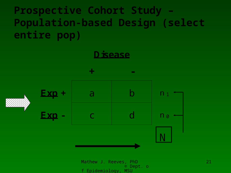
Types of Cohort Studies

• Population-based (one-sample)• select entire popl (N) or known fraction of popl (n)• p (Exposed) in population can be determined

• Multi-sample• select subgroups with known exposures

– e.g., smokers and non-smokers

– e.g., coal miners and uranium miners

• p (Exposed) in population cannot be determined


21

Disease

+ -

Exp + a b n 1

Exp - c d n 0

N

Prospective Cohort Study – Population-based Design (select entire pop)


22

Disease

+ -

Exp + a b n 1

Exp - c d n 0

Prospective Cohort Study – Multi-sample Design (select specific exposure groups)

Rate= c/ n 0

Rate= a/ n 1


23

Exposed

Eligible subjects

Unexposed

Disease

Disease

No disease

No disease

FUTURENOW


24

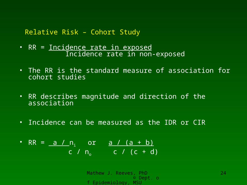
Relative Risk – Cohort Study

• RR = Incidence rate in exposed Incidence rate in non-exposed

• The RR is the standard measure of association for cohort studies

• RR describes magnitude and direction of the association

• Incidence can be measured as the IDR or CIR

• RR = a / ni or a / (a + b) c / noc / (c + d)


25

Example - Smoking and Myocardial Infarction (MI)

MI

+ -

Smk + 30 970 Rate = 30 / 1000

Smk - 10 990 Rate = 10 / 1000

RR= 3

Study: Desert island, pop= 2,000 people, smoking prevalence= 50%Population-based cohort study. Followed for one year. What is the risk of MI among smokers compared to non-smokers?


26

RR - Interpretation

• RR = 1.0 • indicates the rate (risk) of disease among exposed and non-

exposed (= referent category) are identical (= null value)

• RR = 2.0 • rate (risk) is twice as high in exposed versus non-exposed

• RR = 0.5• rate (risk) in exposed is half that in non-exposed


27

RR - Interpretation

• RR = > 5.0 or < 0.2 • BIG

• RR = 2.0 – 5.0 or 0.5 – 0.2 • MODERATE

• RR = <2.0 or >0.5• SMALL


28

Sources of Cohorts

• Geographically defined groups:• Framingham, MA (sampled 6,500 of 28,000, 30-50 yrs of

age)• Tecumseh, MI (8,641 persons, 88% of population)

• Special resource groups• Medical plans e.g., Kaiser Permanente• Medical professionals e.g.,

• Physicians Health Study, Nurses Health Study

• Veterans• College graduates e.g., Harvard Alumni


29

Sources of Cohorts

• Special exposure groups• Occupational exposures

– e.g., pb workers, U miners – If everyone exposed then need an external cohort

non-exposed cohort for comparison purposes– e.g., compare pb workers to car assembly workers

• Specific risk factor groups – e.g., smokers, IV drug users, HIV+


30

Cohort Design Options

• variation in timing of E and D measurement

Design Past

Prospective

Retrospective

Historical/pros.

E D

E E D

DE

Present Future


31

Disease

+ -

Exp + a b n 1

Exp - c d n 0

Retrospective Cohort Study – DesignGo back and determine exposure status based on historical information and then classify subjects according to their current disease status

Rate= c/ n 0

Rate= a/ n 1


32

Exposed

Eligible subjects

Unexposed

Disease

Disease

No disease

No disease

NOWPAST RECORDS


33

Examples retrospective cohort

• Aware of cases of fibromyalgia in women in a large HMO. Go back and determine who had silicone breast implants (past exposure). Compare incidence of disease in exposed and non-exposed.

• Framingham study: use frozen blood bank to determine baseline level of hs-CRP and then measure incidence of CHD by risk groups (quartile)


34

PAR and PARF

• Important question for public health • How much can we lower disease incidence if we intervene

to remove this risk factor?

• Want to know how much disease an exposure causes in a population.

• PAR and PARF assume that the risk factor in question is causal

• See Lecture 3 course notes


35

Venous thromboemolic disease (VTE) and oral contraceptives (OC) in woman of

reproductive age

• Incidence of VTE:• OC users: 16 per 10,000 person-years • non-OC users: 4 per 10,000 person-years• Total population: 7 per 10,000 person-years

• RR = 16/4 = 4

• Prevalence of exposure to OC: • 25% of woman of reproductive age


36

Population attributable risk (PAR)

• The incidence of disease in a population that is associated with a risk factor.

• Calculated from the Attributable risk (or RD) and the prevalence (P) of the risk factor in the population• PAR = Attributable risk x P• PAR = (16-4) x 0.25• PAR = 3 per 10,000 person years

• Equals the excess incidence of VTE in the population due to OC use


37

Population attributable risk fraction (PARF)

• The fraction of disease in a population that is attributed to a risk factor.

• PARF = PAR/Total incidence • PARF = 3/7per 10,000 person years• PARF = 43%

• Represents the maximum potential impact on disease incidence if risk factor was removed• So, remove OC’s and incidence of VTE drops 43% in women of

repro age (assuming OC is a cause of VTE)


38

Exposed

Eligible subjects

Unexposed

Disease

Disease

No disease

No disease

FUTURENOW

PARF = -


39

PARF Calculation

• PARF = P(RR-1)/ [1 + P(RR-1)]where:

• P = prevalence, RR = relative risk

• PARF = 0.25(4-1)/ [1 + 0.25(4-1)]• PARF = 43%

• Note that a factor with a small RR but a large P can cause more disease in a population than a factor with a big RR and a small P.


40

Selection Bias

• Selection bias can occur at the time the cohort is first assembled: • Patients assembled for the study differ in ways other than the

exposure under study and these factors may determine the outcome

– e.g., Only the Uranium miners at highest risk of lung cancer (i.e., smokers, prior family history) agree to participate

• Selection bias can occur during the study• e.g., differential loss to follow-up in exposed and un-exposed

groups (same issue as per RCT design)• Loss to follow-up does not occur at random

• To some degree selection bias is almost inevitable.


41

Confounding Bias• Confounding bias can occur in cohort studies

because the exposure of interest is not assigned at random and other risk factors may be associated with both the exposure and disease.

• Example: cohort study of lecture attendance

Attendance Exam success

Baseline epi proficiency

-

- +


42

Cohort Studies - Advantages

• Can measure disease incidence • Can study the natural history • Provides strong evidence of casual association between E

and D (time order is known)• Provides information on time lag between E and D• Multiple diseases can be examined• Good choice if exposure is rare (assemble special exposure

cohort) • Generally less susceptible to bias vs. CCS


43

Cohort Studies - Disadvantages

• Takes time, need large samples, expensive• Complicated to implement and conduct• Not useful for rare diseases/outcomes • Problems of selection bias

• At start = assembling the cohort• During study = loss to follow-up

• With prolonged time period:• loss-to-follow up• exposures change (misclassification)

• Confounding• Exposures not assigned at random


44

Prognostic Studies - predicting outcomes in those with disease

• Also measured using a cohort design (of affected individuals)

• Factors that predict outcomes among those with disease are called prognostic factors and may be different from risk factors.

• Discussed further in Epi-547

Documents

Mathew J. Reeves, PhD © Dept. of Epidemiology, MSU 1 Lecture 8 – Study Design I XS and Cohort Studies Mathew J. Reeves BVSc, PhD Associate Professor, Epidemiology