Embed Size (px)
Citation preview

Mathematisches Forschungsinstitut Oberwolfach
Report No. 34/2012
DOI: 10.4171/OWR/2012/34
Discrete Differential Geometry
Organised byAlexander I. Bobenko, BerlinRichard Kenyon, ProvidencePeter Schroder, Pasadena
Gunter M. Ziegler, Berlin
July 8th– July 14th, 2012
Abstract. This is the collection of extended abstracts for the 24 lecturesand the open problems session at the third Oberwolfach workshop on DiscreteDifferential Geometry.
Mathematics Subject Classification (2010): 52-xx, 53-xx, 57-xx.
Introduction by the Organisers
Discrete Differential Geometry is a very productive research area where graphtheory, analysis, integrability, and geometry interact and contribute to the con-struction and understanding of discrete models for differential geometric situationsand structures. It also plays a very important role in applications, to graphics andsimulations of PDE.
This was the third Discrete Differential Geometry conference at Oberwohlfach.The subject has evolved significantly since its beginning a decade ago. This year’sconference highlighted advances in new areas: in discrete exterior calculus andcluster algebras in geometry, as well as in some older ones: discrete uniformization,polyhedra, applications to PDE.
The workshop featured many talks around the subject of discrete exterior cal-culus. The main idea of discrete exterior calculus is to find the right adaptation ofthe classical notions of forms, exterior differentiation, Hodge decomposition, etc.to functions on cell complexes, with the goal being to do classical analysis usingdiscrete approximations to continuous objects. The talks by Chelkak, von Deylen,Gunther, Hildebrandt, Skopenkov, Stern all fit in this category. From the variety

2078 Oberwolfach Report 34/2012
of techniques presented we can only say that the subject is still under discussion,and that a global framework is still to be found.
Another new and exciting direction is the integrability and cluster structure ofdiscrete geometric mappings. Here we heard talks by Doliwa, Goncharov, Suris,Tabachnikov on connections between various discrete systems and cluster alge-bras/varieties or other integrable structures. This area seems ripe for furtherexploration, in particular since we don’t understand what features these modelshave in common, and what consequences the cluster structure may have. In par-ticular the cluster structure allows one to introduce quantization which may yieldimportant new avenues of research.
There were a few talks about polyhedra (by Adiprasito, Izmestiev, Schlenker)and versions of discrete uniformization (by Sechelmann, Stephenson, Sullivan).Although these are more well-studied areas the new ideas presented open newopportunities for further research.
Finally there were a few talks about discretizations of PDE: by Crane, Lessig,Schief, Schumacher, Hoffmann, Vouga. Here we include applications to graphics:mapping textures to surfaces and smoothing using conformal maps is one commontheme. This area of PDE applications continues to be an important source ofinspiration for theoretical advances in discrete differential geometry: our goal isto be able to model PDEs, and often finding the right discretization makes a hugedifference in efficiency. Furthermore some systems have discretizations which arein some sense more natural than their continuous counterparts (in the sense thatthere is more mathematical structure).
The organizers are grateful to all participants for all the lectures, discussions,and conversations that combined into this very lively and successful workshop –and to everyone at Research Institute in Oberwolfach for the perfect setting.

Discrete Differential Geometry 2079
Workshop: Discrete Differential Geometry
Table of Contents
Karim A. Adiprasito (joint with Gunter M. Ziegler)Many 4-polytopes with a low-dimensional realization space . . . . . . . . . . . . 2081
Dmitry ChelkakDiscrete complex analysis: conformal invariants without conformalinvariance . . . . . . . . . . . . . . . . . . . . . . . . . . . . . . . . . . . . . . . . . . . . . . . . . . . . . . 2083
Keenan Crane (joint with Clarisse Weischedel and Max Wardetzky)Fast Computation of Geodesic Distance via Linear Elliptic Equations . . 2086
Stefan W. von DeylenAxioms for an Arbitrary (Discrete) Calculus with Dirichlet Problem andHodge Decomposition . . . . . . . . . . . . . . . . . . . . . . . . . . . . . . . . . . . . . . . . . . . . 2087
Adam DoliwaHirota equation and the quantum plane . . . . . . . . . . . . . . . . . . . . . . . . . . . . . 2089
Felix Gunther (joint with Alexander I. Bobenko)Discrete complex analysis on quad-graphs . . . . . . . . . . . . . . . . . . . . . . . . . . . 2091
Klaus Hildebrandt (joint with Konrad Polthier)Consistent discretizations of the Laplace–Beltrami operator and theWillmore energy of surfaces . . . . . . . . . . . . . . . . . . . . . . . . . . . . . . . . . . . . . . 2094
Wolfgang K. Schief and Tim HoffmannDiscrete focal surfaces and geodesics . . . . . . . . . . . . . . . . . . . . . . . . . . . . . . . 2097
Ivan IzmestievFlexible Kokotsakis polyhedra and elliptic functions . . . . . . . . . . . . . . . . . . 2099
Christian LessigThe Geometry of Light Transport Theory . . . . . . . . . . . . . . . . . . . . . . . . . . . 2100
Yaron LipmanDiscrete Quasiconformal Mappings of Triangular Meshes . . . . . . . . . . . . . 2103
Feng LuoSimplicial SL(2,R) Chern-Simons theory and Boltzmann entropy ontriangulated 3-manifolds . . . . . . . . . . . . . . . . . . . . . . . . . . . . . . . . . . . . . . . . . . 2103
Stefan Sechelmann (joint with Alexander I. Bobenko and Boris Springborn)Uniformization of discrete Riemann surfaces . . . . . . . . . . . . . . . . . . . . . . . . 2105
Jean-Marc Schlenker (joint with Jeffrey Danciger and Sara Maloni)Geometric properties of anti-de Sitter simplices and applications . . . . . . . 2107

2080 Oberwolfach Report 34/2012
Henrik Schumacher (joint with Sebastian Scholtes and Max Wardetzky)Convergence of Discrete Elastica . . . . . . . . . . . . . . . . . . . . . . . . . . . . . . . . . . 2108
Mikhail SkopenkovDiscrete analytic functions: convergence results . . . . . . . . . . . . . . . . . . . . . 2110
Olga Sorkine (joint with Daniele Panozzo, Olga Diamanti, Ilya Baran)Weighted Averages on Surfaces . . . . . . . . . . . . . . . . . . . . . . . . . . . . . . . . . . . . 2111
Ken Stephenson (joint with James Ashe and Edward Crane)Generalized Branching: Making Circles Behave . . . . . . . . . . . . . . . . . . . . . . 2113
Ari Stern (joint with Paul Leopardi)The abstract Hodge–Dirac operator and its stable discretization . . . . . . . . 2116
John M. SullivanLifting Spherical Cone Metrics . . . . . . . . . . . . . . . . . . . . . . . . . . . . . . . . . . . . 2118
Yuri B. Suris (joint with Matteo Petrera)Spherical geometry and integrable systems . . . . . . . . . . . . . . . . . . . . . . . . . . 2122
Serge TabachnikovHigher pentagram maps, directed weighted networks, and cluster algebras 2125
Etienne Vouga (joint with Mathias Hobinger, Johannes Wallner, HelmutPottmann)Design of Self-supporting Surfaces . . . . . . . . . . . . . . . . . . . . . . . . . . . . . . . . . 2127
Collected by Klaus HildebrandtOpen problems in Discrete Differential Geometry . . . . . . . . . . . . . . . . . . . . 2130

Discrete Differential Geometry 2081
Abstracts
Many 4-polytopes with a low-dimensional realization space
Karim A. Adiprasito
(joint work with Gunter M. Ziegler)
We report on recent progress [1] on two classical problems concerning the spaceof geometric realizations of a given polytope. The first problem seems to originatewith Perles. A d-polytope P ∈ Rd is projectively unique if every polytope P ′ in Rd
combinatorially equivalent to P is related to P via a projective transformation.
Problem I (Perles & Shephard ’74 [8], Kalai ’97 [5]). Is it true that, for fixedd, the number of distinct combinatorial types of projectively unique d-polytopes isfinite?
It was generally conjectured that the answer to this problem is positive, eventhough no substantial progress was made since 1976 [7]. It is easy to see thata 2-polytope is projectively unique if and only if it has 3 or 4 vertices. Thecase of 3-polytopes is more demanding. Classical approaches highlight the closeconnection of Problem I to the dimension of the realization space RS(P ) (cf. [12])of a polytope P .
Theorem 1 (Legendre–Steinitz Formula [11, Sec. 69, p. 349]). The realizationspace of a 3-polytope P is of dimension f1(P ) + 6.
From this, we can see that a 3-polytope can be projectively unique only iff1(P ) + 6 ≤ dimPGL(R4) = 15. A more careful analysis reveals that this is infact a complete characterization: A 3-polytope is projectively unique if and onlyif it has at most 9 edges [3, Sec. 4.8, pr. 30].
This argument motivates the study of the dimension of the realization space ofa polytope as a separate problem, which goes back to research of Legendre. Hewas the first to give the correct formula (Theorem 1) for the dimension of therealization space of 3-polytopes, cf. [6, Note VIII, p. 309], the first proof for whichwas later supplied by Steinitz [11, Sec. 69].
Let the size of a polytope be given by the combined number of its vertices andfacets. We study Legendre’s problem in the following form:
Problem II (Legendre–Steinitz; cf. Ziegler 2011 [12]). How does, for d-dimensionalpolytopes, the dimension of the realization space grow with the size of the polytopes?
Main Idea and Results. Our approach to these problems is given by the ob-servation that the 8-th vertex of a realization of the 3-cube is determined by theremaining 7 vertices. This idea gives rise to a construction technique for cubicalcomplexes as follows: We give a sequence of cubical 3-complexes Tn, n ∈ N, calledtransmitters, such that for every construction step Tn−1 → Tn, Tn is obtained fromTn−1 by attaching a (combinatorial) 3-cube W to Tn−1 such that Tn−1 ∩W has7 vertices. Since the geometric realization of the attached cube is determined by

2082 Oberwolfach Report 34/2012
the information in Tn−1, the geometric realization of Tn is determined by the re-alization of Tn−1, and in particular, the geometric realization of Tn is determinedby the realization of T0.
With this technique, we are able to complete the answer to Problem II.
Theorem I (Transmitter polytopes, A.-Ziegler [1]). There is an infinite family(TRP4[n]), n ∈ N of combinatorially distinct 4-dimensional polytopes on 24 + nvertices, such that for all n, dimRS(TRP4[n]) is bounded above by 96.
As an immediate corollary, we obtain:
Corollary 1. For each d ≥ 4, there is an infinite family (TRPd[n]), n ∈ N ofcombinatorially distinct d-dimensional polytopes such that dimRS(TRPd[n]) ≤76 + d(d + 1) for all n.
Building on the family (TRP4[n]), we can use extension techniques, in particularLawrence extensions (see for example [9]), to answer Problem I for all dimensionshigh enough.
Theorem II (Rigid transmitter polytopes, A.-Ziegler [1]). There is an infinitefamily (RTP81[n]), n ∈ N of combinatorially distinct 81-dimensional polytopes, allof which are projectively unique.
Again, we can immediately conclude:
Corollary 2. For each d ≥ 81, there is an infinite family (RTPd[n]), n ∈ N
of combinatorially distinct d-dimensional polytopes, all of which are projectivelyunique.
The hardest part of the proof of Theorem I (and Theorem II) goes into ageometric construction of a complex T0 that allows for the repeated attachment of3-cubes in accordance with our construction technique. The pivotal structure forthis initial complex T0 is formed by (weighted) Clifford tori, upon which we buildthe sequence of complexes Tn, all of which are homeomorphic to T 2×I, and whosevertices are, in turn, distributed over several weighted Clifford tori in a symmetricfashion. For the study of T0 and its extensions Tn, Santos [10] provided valuableintuition.
To ensure that the extensions Tn of T0 give rise to 4-polytopes, we use the notionof convex position complexes which is closely related to the theory of (locally)convex hypersurfaces, cf. [2, 4]. Convex position encodes the property of beingthe subcomplex of the boundary complex of a convex polytope. Using a carefuladaption of the Alexandrov–van Heijenoort Theorem to manifolds with boundary,we prove that our complexes Tn are indeed in convex position, and consequentlygive rise to convex polytopes by considering the polytopes TRP4[n] := conv Tn.
To finish the proof, we then note that the realization space of the polytopesTRP4[n] is naturally embedded into the realization space of Tn, which in turnis embedded into the realization space of T0. In particular, dimRS(TRP4[n]) ≤dimRS(Tn) ≤ dimRS(T0), and dimRS(TRP4[n]) is uniformly bounded. A morecareful analysis gives the bound of Theorem I.

Discrete Differential Geometry 2083
References
[1] K. Adiprasito and G. M. Ziegler, On polytopes with low-dimensional realization spaces. Inpreparation (2012).
[2] A. D. Aleksandrov, Intrinsic geometry of convex surfaces. OGIZ, Moscow-Leningrad, 1948.[3] B. Grunbaum, Convex polytopes. Graduate Texts in Mathematics 221, Springer-Verlag, New
York, second ed. 2003.[4] J. van Heijenoort, On locally convex manifolds. Comm. Pure Appl. Math. 5 (1952), 223–242.
[5] G. Kalai, Polytope skeletons and paths. Handbook of Discrete and Computational Geometry(J. E. Goodman and J. O’Rourke, eds.), Chapman & Hall/CRC, Boca Raton, FL, seconded. 2004, 455–476.
[6] A. M. Legendre, Elements de geometrie. Imprimerie de Firmin Didot, Paris 1794, twelfthed. 1823 http://archive.org/details/lmentsdegomtrie10legegoog.
[7] P. McMullen, Constructions for projectively unique polytopes. Discrete Math. 14 (1976),347–358.
[8] M. A. Perles and G. C. Shephard, A construction for projectively unique polytopes. Geome-triae Dedicata 3 (1974), 357–363.
[9] J. Richter-Gebert, Realization spaces of polytopes. Lecture Notes in Mathematics 1643,Springer-Verlag, Berlin, 1996.
[10] F. Santos, A counterexample to the Hirsch conjecture. Ann. of Math. 176 (2012), 383–412.[11] E. Steinitz and H. Rademacher, Vorlesungen uber die Theorie der Polyeder unter Einschluss
der Elemente der Topologie. Springer-Verlag, 1934.[12] G. M. Ziegler, Polytopes with low-dimensional realization spaces (joint work with K. Adipr-
asito). Oberwolfach Rep. 8 (2011), 2522–2525.
Discrete complex analysis: conformal invariants without conformalinvariance
Dmitry Chelkak
Dealing with some 2D lattice model and its scaling limit (e.g., with the 2D Brow-nian motion in a fixed planar domain, which can be realized as a limit of randomwalks on refining lattices δZ2), one usually works in the context when the lat-tice mesh δ tends to zero. Then, one can argue that a pre-limiting behavior ofthe model is sufficiently close to the limiting one, if δ is small enough, e.g., therandom walks hitting probabilities (discrete harmonic measures) become close tothe Brownian motion hitting probabilities (classical harmonic measure) as δ → 0.After re-scaling by δ−1, such statements provide an information about randomwalk properties in (the bulk of) large discrete domains in Z2.
In this talk, we are interested in uniform estimates which hold true for arbitrarydiscrete domains, possibly having many fiords and bottlenecks of various widths,including very thin (several lattice steps) ones. Having in mind the classical geo-metric complex analysis as a guideline, we would like to construct its discreteversion “staying on a microscopic level” (i.e., without any limit passage), whichallows one to handle discrete domains by the same methods as continuous ones.
The main objects of our interest are discrete quadrilaterals, i.e. simply con-nected domains Ω with four marked boundary points a, b, c, d. Focusing on quadri-laterals, we are motivated by two reasons. First, in the classical theory this is the“minimal” configuration which has a nontrivial conformal invariant (e.g., all simply

2084 Oberwolfach Report 34/2012
connected domains with three marked boundary points are conformally equivalentdue to the Riemann mapping theorem). Second, quadrilaterals are archetypicalconfigurations for the 2D lattice models theory, where one often needs to estimatethe probability of some crossing-type event between the opposite boundary arcs[ab], [cd] ⊂ ∂Ω of a discrete simply connected domain Ω.
Below we present a number of uniform double-sided estimates (1)–(3) relatingdiscrete counterparts of several classical conformal invariants of a configuration(Ω; a, b, c, d): cross-ratios, random walk partition functions and extremal lengths.
Let Ω be a discrete domain (i.e., connected subset of Z2) and A,B ⊂ ∂Ω. Wedenote by ZΩ(A;B) the total partition function of the simple random walk runningfrom A to B inside Ω. Namely,
ZΩ(A;B) = ZΩ(B;A) :=∑
γ∈SΩ(a;b)
4−Length(γ),
where SΩ(A;B) = γ = (u0u1 . . . un) : u0 ∈ A, u1, . . . , un−1 ∈ IntΩ, un ∈ B isthe set of all nearest-neighbor paths connecting A and B in Ω, and Length(γ) = n.
Further, let Ω be a simply-connected discrete domain and a, b, c, d ∈ ∂Ω be fourboundary points listed counterclockwise. We define their discrete cross-ratios by
XΩ(a, b; c, d) :=
[ZΩ(a; c) · ZΩ(b; d)
ZΩ(a; b) · ZΩ(c; d)
] 12
, YΩ(a, b; c, d) :=
[ZΩ(a; d) · ZΩ(b; c)
ZΩ(a; b) · ZΩ(c; d)
] 12
.
Note that the continuous analogue of the partition function ZΩ(a; b) for the upperhalf-plane Ω = H (up to a multiplicative constant) is given by (b − a)−2, so thequantities introduced above are discrete counterparts of the usual cross-ratios
xH(a, b; c, d) :=(b−a)(d−c)(d−b)(c−a) , yH(a, b; c, d) :=
(b−a)(d−c)(d−a)(c−b) .
Moreover, for any continuous Ω, the corresponding xΩ, yΩ could be definedvia a proper conformal mapping Ω → H. In particular, one has the standardidentity x−1
Ω = 1+ y−1Ω for any (Ω; a, b, c, d). Since in the discrete setup there is no
appropriate notion of conformal invariance (for different subsets of the fixed grid),one cannot hope that this identity remains valid for discrete Ω’s. Nevertheless, itturns out that the similar uniform double-sided estimate holds true:
(1) XΩ(a, b; c, d)−1 ≍ 1 + YΩ(a, b; c, d)
−1,
i.e., there exist two independent of Ω, a, b, c, d constants C1, C2 > 0 such thatC1X
−1Ω ≤ 1 + Y−1
Ω ≤ C2X−1Ω for all possible discrete quadrilaterals (Ω; a, b, c, d).
Further, note that the natural continuous analogues zΩ([ab]; [cd]) of the totalpartition functions ZΩ([ab]; [cd]) are conformally invariant as well, and, for Ω = H,one has (up to a multiplicative constant)
zH([ab]; [cd]) = log(c− a)(d − b)
(d− a)(c− b)= log(1 + yH(a, b; c, d)).
Hence, this identity is fulfilled for any continuous quadrilateral (Ω; a, b, c, d). Again,it cannot survive on the discrete level, but one can prove that the similar uniform

Discrete Differential Geometry 2085
double-sided estimate
(2) ZΩ([ab]; [cd]) ≍ log(1 + YΩ(a, b; c, d))
holds true for discrete quadrilaterals (with constants independent of (Ω; a, b, c, d)).In order to summarize our results, it is worthwhile to introduce the third quan-
tity related to a discrete quadrilateral which is a well known discrete analogue ofthe extremal length notion. Let E(Ω) be the set of all edges of Ω. We define
LΩ([ab]; [cd]) := supw:E(Ω)→R+
minγ⊂E(Ω):[ab]↔[cd]
(∑e∈γ w(e)
)2
∑e∈E(Ω)(w(e))
2,
where min is taken over all nearest-neighbor paths γ connecting [ab] and [cd] in Ωand sup is over all nonnegative functions (“discrete metrics”) w : E(Ω) → R+.
Note that one can easily estimate extremal lengths since for this purpose it issufficient to take any “discrete metric” w0 in Ω (possibly, having some naturalgeometric meaning) and estimate the corresponding ratio for this particular w0.Our main results are summarized in the following
Theorem. Let Ω be a simply connected discrete domain and boundary pointsa, b, c, d ∈ ∂Ω be listed in the counterclockwise order. Denote
Y := YΩ(a, b; c, d), Z := ZΩ([ab]; [cd]), L := LΩ([ab]; [cd]);
Y′ := YΩ(b, c; d, a), Z′ := ZΩ([bc]; [da]), L′ := LΩ([bc]; [da]).
Then, the following uniform estimates are fulfilled:
(3)log(1 + Y) ≍ Z ≤ L−1
Y · Y′ = 1 L · L′ ≍ 1log(1 + Y′) ≍ Z′ ≤ (L′)−1
Moreover, Z′ ≍ (L′)−1, if L′ ≤ const < +∞ (or, equivalently, L ≥ const > 0).
Finally, note that the most essential ingredient of our proofs is the asymptotics
G(u;u0) =1
2πlog |u− u0|+O(1)
of the free Green’s function which is known (in a much more precise form) at leastfor the class of isoradial graphs. Thus, if this asymptotics is established for someclass of planar graphs, one almost immediately has a “toolbox” described above(for this class of graphs) which allows one to use classical methods of geometriccomplex analysis more-or-less in the same style as in the usual continuous setup.

2086 Oberwolfach Report 34/2012
Fast Computation of Geodesic Distance via Linear Elliptic Equations
Keenan Crane
(joint work with Clarisse Weischedel and Max Wardetzky)
The geodesic distance φ to a point x on a Riemannian manifold M is typicallycharacterized in terms of the nonlinear hyperbolic eikonal equation |∇φ| = 1.We present an alternative formulation in terms of linear elliptic equations, whichhas important practical and numerical consequences. In particular, let ∆ be the(negative-semidefinite) Laplace-Beltrami operator onM and let δ be a Dirac deltacentered at x. The heat kernel is the solution to the heat equation
u = ∆u
with initial conditions u0 = δ. As observed by Varadhan [1],
φ = limt→0
√−4t logut,
i.e., the geodesic distance can be recovered as the limit of a simple pointwisetransformation applied to the heat kernel. In practice, however, it is difficult toobtain a precise numerical reconstruction of ut.
Consider instead the single-step backward Euler approximation of the heat ker-nel given by the solution to the linear elliptic equation
(id− t∆)vt = δ
for a fixed integration time t, where id is the identity operator. Since the functionvt is merely a crude approximation of the true heat kernel ut, applying Varadhan’stransformation no longer yields the geodesic distance. It can be shown, however,that limt→0 vt is a monotonically decreasing function of the distance to x, whichmeans that ∇vt will become parallel to the gradient of the distance function ∇φas t→ 0. Alternatively, if we define X := −∇vt/|∇vt| then we have
limt→0
X = ∇φ,
since (as indicated by the eikonal equation) ∇φ has unit length. For finite values oft the vector field X may not be integrable, but we can obtain a close approximation
φ of φ by solving the problem
minφ
|∇φ −X |2,
or equivalently, by solving
∆φ = ∇ ·Xwhich is a standard linear elliptic Poisson equation. These observations lead to the
heat method, which can be used to obtain a consistent approximation φ of geodesic
distance (i.e., limt→0 φ = φ):
Computationally this method is attractive because the linear equations fromsteps (I) and (III) can easily be prefactored and solved in parallel; step (II) is

Discrete Differential Geometry 2087
Algorithm 1 The Heat Method
I. Solve (id− t∆)vt = δ.II. Evaluate X = −∇vt/|∇vt|.III. Solve ∆φ = ∇ ·X .
a simple pointwise evaluation. Further discussion of the method (including dis-cretization and numerics) can be found in [2].
References
[1] S. Varadhan, On the behavior of the fundamental solution of the heat equation with variablecoefficients. Communications on Pure and Applied Mathematics 20 (1967), 431–455.
[2] K. Crane, C. Weischedel, and M. Wardetzky, Geodesics in heat. arXiv:1204.6216v1.
Axioms for an Arbitrary (Discrete) Calculus with Dirichlet Problemand Hodge Decomposition
Stefan W. von Deylen
Consider am Riemannian manifold (M, g). The Dirichlet problem is to findminimisers of the Dirichlet energy Dir(u) = 〈du, du〉L2 + 〈δu, δu〉L2 inside anappropriate class of functions or differential forms. The (L2-orthogonal) Hodgedecomposition of any vector field α as
α = dφ+ δχ+ ψ such that dψ = 0, δψ = 0
subject to some additional conditions on the boundary values of φ, χ and ψ, isstrongly connected to the unique solvability of the Dirichlet problem. For bothproblems, it is well known that the space of Sobolev differential forms H1Ωk(M)is the appropriate choice of regularity, see [4].
There are several approaches to define “discrete exterior calculi”, see e. g. [3, 2,1]. Sometimes by interpolation properties, sometimes by mere discrete calculation,they show that the above properties of the continous calculus are reflected in theirdefinitions.
We have asked ourselves for the “minimal set of definitions” that is fulfilled byall these discrete constructions as well as their smooth counterpart and proposethe following:
Definition. SupposeM is an n-dimensional compact, oriented cone manifold withboundary. An exterior calculus (Gk,Ω
k) consists of
(a) collections G1, . . . , Gn of “integration domains”: each U ∈ Gk is a smooth k-dimensional submanifold of M such that ∂U can be covered by Gk−1 domains.
(b) L2-closed spaces Ω0, . . . ,Ωn of differential forms such that Ωk ⊂ L2Ωk(M)and each α ∈ Ωk is integrable on each U ∈ Gk.

2088 Oberwolfach Report 34/2012
This definition collects all objects that are needed to form a calculus. Let us addsome purely notational definitions: A form is some α ∈ Ωk weakly differentiableif there is dα ∈ Ωk+1 with
∫
U
dα =
∫
∂U
α for all U ∈ Gk+1.
Call dα the weak exterior derivative of α (if it is not unique, pick the one withleast L2 norm). The pointwise projection of α onto the tangent space of a lower-dimensional submanifold, e. g. ∂U , (the “tangential part”) is denoted as tα, theprojection onto the orthogonal complement (the “normal part”) as nα.
Of course, one can construct very strange collections of forms and domains thatdo not have much to do with one another. As conditions for an exterior calculusto be “useable”, we propose the following:
(a) the space H1Ωk of weakly differentiable Ωk forms should be dense in Ωk,(b) there is a co-differential δ with 〈α, dβ〉L2 = 〈δα, β〉L2 if tβ = 0 or nα = 0,(c) but if nα 6= 0, there is β with 〈α, dβ〉L2 6= 〈δα, β〉L2 and vice versa for tβ 6= 0.
Remark that in general this co-differential δ is not neccessarily linked to thedifferential by the Hodge star, δ 6= ∗d∗.Comparison. The fact that Ωk may also be spaces of piecewise constant differ-ential forms and yet admit a weak derivative in the above sense, as the Stokes’formula only has to hold on a very limited set of domains, has some implicationsfor the comparison to other discrete calculi.
(1.) The FEEC (finite element exterior calculus) approach, cf. [1] and AriStern’s abstract in this report, needs weakly differentiable forms in the usualSobolev sense, e. g. piecewise smooth and globally continous forms. One wayto see our definition is to make their approach applicable to the purely discreteapproaches, e. g.:
(2.) The DEC (discrete exterior calculus) approach, cf. [2], does (at leastin the first step) not define k-forms in the usual sense, but only numbers at k-cells. When some interpolation is chosen, mostly piecewise linear and globallycontinous (Whitney forms), Stokes’ and Green’s theorem do not neccessarily holdon the level of interpolating forms. But an appropriately chosen piecewise constantinterpolation keeps both theorems valid, and it will be weakly differentiable in theabove definition, thus admitting the results given below without extra proofs forthe discrete setting.
Result. The reason that we consider these objects above as a “minimal set” ofobjects to form an exterior calculus is that a careful inspection of the Sobolevtheory for the aforementioned problems, Dirichlet problem and the Hodge decom-position, e. g. from [4], shows that all their proofs will carry over. We especiallyemphasise that the following properties of any “useable” exterior calculus areproven by literally taking over the proofs from Sobolev theory:
Theorem. Let (Gk,Ωk) be a “useable” exterior calculus as above. Then hold for
H k := α ∈ Ωk | Dir(α) = 0:

Discrete Differential Geometry 2089
(a) Dirichlet problem: For each f ∈ (H kt)⊥, there is a unique u ∈ (H k
t)⊥twith
〈dα, dψ〉+ 〈δα, δψ〉 = 〈f, ψ〉 for all ψ ∈ Ωkt.
(b) Hodge decomposition: Ωk = d(Ωk−1t
)⊕ δ(Ωk+1n
)⊕ H k
(c) Friedrichs decomposition: H k = H kn⊕H k∩d(Ωk−1) = H k
t⊕H k ∩δ(Ωk+1)
(d) kerdk/ im dk−1 ≃ H kn
(e) de Rham: if spanR
(Gk) is a dense subspace of (Ωk)′, then ker ∂k/ im∂k+1 ≃kerdk/ im dk−1
References
[1] Arnold, D. N, Falk, R. S., and Winther R., Finite element exterior calculus: From Hodgetheory to numerical stability. Bulletin of the AMS 47 (2010), pp. 281–354.
[2] Desbrun, M., Kanso, E., and Tong, Y., Discrete differential forms for computational mod-eling. In: ACM SIGGRAPH Asia 2008 courses, New York: ACM 2008, pp. 46–67.
[3] Polthier, K. and Preuss, E., Variational approach to vector field decomposition. In: Scien-tific Visualization (Proceedings of the Eurographics Workshop on Scientific VisualizationAmsterdam 2000), Springer, Berlin 2000.
[4] Schwarz, G., Hodge decomposition – A Method for Solving Boundary Value Problems. Lec-ture Notes in Mathematics 1607, Berlin, Springer 1995.
Hirota equation and the quantum plane
Adam Doliwa
Hirota’s discrete Kadomtsev–Petviashvili equation [5] may be considered as theHoly Grail of integrable systems theory, both on the classical and the quantumlevel [6]. Its geometric interpretation is provided [2] by Desargues maps (seeFigure 1). These are the maps φ : ZK → PM (D) of multidimensional integerlattice into projective space (over a division ring D) subject to collinearity of alltriplets of points φ(n), φ(i)(n) and φ(j)(n), i 6= j; here φ(i)(n1, . . . , ni, . . . , nK) =φ(n1, . . . , ni + 1, . . . , nK). We remark that the symmetry properties of Desarguesmaps are more transparent [3] in the language of the AK root lattice and of thecorresponding affine Weyl group.
Geometric integrability of the maps follows from the celebrated Desargues the-orem. In algebraic terms the nonlinear system generated by Desargues maps (anon-commutative Hirota equation) can be decomposed [4] into reiterated applica-tion of two maps, which are solutions of the functional pentagon equation. Thesimpler one W : D2 × D2 ∋ ((x1, y1), (x2, y2)) 99K ((x1, y1), (x2, y2)) ∈ D2 × D2
x1 = x2 + x1y2, y1 = y1y2(1)
x2 = −y1x−11 x2, y2 = y2 + x−1
1 x2(2)
is related to collinearity of four points. We stress that the functional pentagonequation
(3) W12 W23 =W23 W13 W12, in D2 × D
2 × D2
is satisfied without any assumptions about commutativity of the multiplication.

2090 Oberwolfach Report 34/2012
φ(ij)
φ
(k)φ
φ(j)
φ(ik)
φ (jk)
(i)φ
Figure 1. Desargues map condition and the Veblen configuration
The second map WG : D2 × D2 99K D2 × D2
u′1 = Gw1, w′1 = w2w1
u′2 = −u2w1u−11 , w′
2 = Gw1u−11
contains a free gauge parameter G, and is directly related to Desargues config-uration. The pentagonal property of the map follows from the symmetry of theconfiguration; on the algebraic level the gauge parameters of the correspondingfive maps have to be suitably adjusted.
We present also a path to the corresponding solutions of the quantum penta-gon equation [1]. In doing the reduction from ”noncommutative to quantum” weelucidate [4] the role of the ultra-locality principle (the tensor product structure)which leads to the Weyl commutation relations
xy = qyx
of the quantum plane Kq[x, y]. Moreover, the pentagonal property of the map Wimplies coassociativity of the coproduct ∆ : Kq[x, y] → Kq[x, y]⊗Kq[x, y]
(4) ∆(x) = 1⊗ x+ x⊗ y, ∆(y) = y ⊗ y,
which should be compared with equation (1). From that it follows the Hopf algebrastructure of the extended quantum plane Kq[x, y, y
−1].
References
[1] S. Baaj, G. Skandalis, Unitaires multiplicatifs et dualite pour les produits croises de C∗-
algebres. Ann. Sci. Ecole Norm. Sup. 26 (1993), 425–488.[2] A. Doliwa, Desargues maps and the Hirota–Miwa equation. Proc. R. Soc. A 466 (2010),
1177–1200.[3] A. Doliwa, The affine Weyl group symmetry of Desargues maps and of the non-commutative
Hirota–Miwa system. Phys. Lett. A 375 (2011), 1219–1224.

Discrete Differential Geometry 2091
[4] A. Doliwa, S. M. Sergeev, The pentagon relation and incidence geometry. arXiv:1108.0944.[5] R. Hirota, Discrete analogue of a generalized Toda equation. J. Phys. Soc. Jpn. 50 (1981),
3785–3791.[6] A. Kuniba, T. Nakanishi, J. Suzuki, T -systems and Y -systems in integrable systems. J.
Phys. A: Math. Theor. 44 (2011), 103001 (146pp).
Discrete complex analysis on quad-graphs
Felix Gunther
(joint work with Alexander I. Bobenko)
We deal with a linear discretization of complex analysis on quad-graphs. Dis-crete holomorphic functions on the square lattice were studied by Isaacs [7], wherehe proposed two different definitions for holomorphicity. One of them was rein-troduced by Ferrand [6] and studied extensively by Duffin [4], who extended thenotion of discrete holomorphicity to rhombic lattices [5]. The investigation of dis-crete complex analysis on rhombic lattices was resumed by Mercat [9], Kenyon [8],Chelkak and Smirnov [3]. For a survey on the theory of discrete complex analy-sis based on circle patterns and its relation to the linear theory, see the book ofBobenko and Suris [2].
Our setting is a bipartite quad-graph Λ corresponding to a strongly regular andlocally finite cell decomposition of a Riemann surface consisting of quadrilateralsonly. Mainly, we are interested in bipartite quad-graphs embedded in the complexplane. We denote by Γ respectively Γ∗ the maximal independent sets of Λ. Inaddition to the graph Λ, its dual ♦ := Λ∗ will come up in the definitions ofdiscrete derivatives.
Being consistent with the previous definitions of discrete holomorphicity, a func-tion H : Λ → C is discrete holomorphic on the face z ∈ ♦, iff
H(u+)−H(u−)
u+ − u−=H(w+)−H(w−)
w+ − w−
for the two diagonals u−u+ and w−w+ of z. Based on this notion of holomorphic-ity, we generalize the discrete derivatives ∂, ∂ of [3] to arbitrary quadrilaterals.These discrete derivatives map functions on Λ to functions on ♦ or vice versa.As in the rhombic setting, we can find discrete primitives of discrete holomorphicfunctions on simply-connected domains of ♦.
For functions on Λ, we show the factorization 4∂∂ = 4∂∂ = where is thediscrete Laplacian introduced by Mercat [10] and studied by Skopenkov [11]. Asa corollary, ∂H is discrete holomorphic if H : Λ → C is discrete harmonic, i.e.H ≡ 0. Also, the real and the imaginary part of a discrete holomorphic functionH : Λ → C are discrete harmonic. Moreover, if H is discrete holomorphic ona simply-connected domain, the imaginary part of H is determined uniquely byits real part up to two additive constants on Γ and Γ∗. In particular, a discreteholomorphic and purely real or purely imaginary functionH on a simply-connecteddomain is constant on Γ and constant on Γ∗.

2092 Oberwolfach Report 34/2012
Skopenkov proved existence and uniqueness of solutions to the discrete Dirichletboundary value problem [11]. Basing on this result, we prove surjectivity of theoperators ∂, ∂,♦ on discrete domains homeomorphic to a disk or the plane. Es-pecially, discrete Green’s functions G(·; v0) : Λ → R and discrete Cauchy kernelsK(·, v0) : ♦ → C and K(·, z0) : Λ → C exist for all v0 ∈ Λ and z0 ∈ ♦ in the casethat Λ discretizes the complex plane. For all v ∈ Λ and z ∈ ♦, these functionsfulfill
G(v0; v0) = 0 and G(v; v0) =1
2µΛ(v0)δvv0 ,
∂K(·; z0) = δzz0π
µ♦(z0)and ∂K(·; v0) = δvv0
π
µΛ(v0).
Here δ is the Kronecker delta, and µΛ(v0) are µ♦(z0) are geometric weights associ-ated to vertices of Λ and ♦ which already appear in the definitions of ∂ and ∂. Notethat we do not require any certain asymptotic behavior. However, we constructdiscrete Green’s functions and Cauchy kernels with asymptotics analogous to therhombic [3, 8] and close to the smooth case if all quadrilaterals are parallelogramswith bounded interior angles and bounded ratio of side lengths. The constructionof these functions is closely related to discrete complex analysis on quasicrystallicparallelogram-graphs [1] and uses the connection to discrete integrable systems [2].
To state discrete Cauchy formulas in a simpler way than in [3], we introduce themedial graph X of Λ which is defined as follows. The vertex set is given by the setof midpoints of all edges of Λ and two vertices are adjacent iff the correspondingedges belong to the same face and have a vertex in common. The set of faces of Xis in bijective correspondence with the vertex set Λ∪♦: A face corresponding to avertex v of Λ consists of the midpoints of all edges incident to v and a quadrilateralface corresponding to a face z of ♦ consists of the four midpoints of edges belongingto z. So given two functions F : ♦ → C and H : Λ → C, we can define a productF ·H on the edges of X in a canonical way. Such functions can then be integratedalong paths of edges of X .
v0
Figure 1. Bipartite quad-graph Λ (dashed) with medial graph X
Note that choosing F ≡ 1 or H ≡ 1, F respectively H is discrete holomorphiciff all closed discrete line integrals of 1 · H respectively F · 1 vanish, yielding a

Discrete Differential Geometry 2093
discrete Morera’s theorem. Also, all closed discrete line integrals of F ·H vanish ifF and H are both discrete holomorphic. Though, F ·H is not everywhere discreteholomorphic in the sense of the theory above. More precisely, F ·H is defined onthe vertices of the medial graph of X , which is the dual of a bipartite quad-graphhaving Λ ∪ ♦ as one maximal independent vertex set and the midpoints of edgesof Λ as the other. But in general, F ·H is discrete holomorphic on the vertices ofΛ ∪ ♦ only.
Let F : ♦ → C and H : Λ → C be discrete holomorphic, and v0 ∈ Λ, z0 ∈ ♦. IfK(·, z0) : Λ → C and K(·, v0) : ♦ → C are discrete Cauchy kernels, then for anydiscrete contour Cz0 or Cv0 on the medial graph X surrounding z0 respectively v0once in counterclockwise order (e.g. the paths determined by the gray vertices inFigure 1), the discrete Cauchy formula holds true:
F (z0) =1
2πi
∮
Cz0
F ·K(·; z0),
H(v0) =1
2πi
∮
Cv0
K(·; v0) ·H.
If additionally Cz0 does not pass through any vertex incident to z0, then
∂H(z0) =1
2πi
∮
Cz0
−∂K(·; z0) ·H.
In the special case of the Z2-lattice of a skew coordinate system in the com-plex plane, ♦ ∼= Λ and all derivatives of a discrete holomorphic functions arediscrete holomorphic themselves. We derive discrete Cauchy formulas for all dis-crete derivatives and show that the nth derivative of the discrete Cauchy kernelwith asymptotics O(x−1) has asymptotics O(x−(n+1)).
References
[1] A.I. Bobenko, C. Mercat and Yu. B. Suris, Linear and nonlinear theories of discrete analyticfunctions. Integrable structure and isomonodromic Green’s function. J. Reine Angew. Math.583 (2005), 117–161.
[2] A.I. Bobenko and Yu.B. Suris, Discrete differential geometry: integrable structures. Grad.Stud. Math. 98, AMS, Providence 2008.
[3] D. Chelkak and S. Smirnov, Discrete complex analysis on isoradial graphs. Adv. Math. 228(2011), 1590–1630.
[4] R.J. Duffin, Basic properties of discrete analytic functions. Duke Math. J. 23 (1956), 335–
363.[5] R.J. Duffin, Potential theory on a rhombic lattice. J. Comb. Th. 5 (1968), 258–272.[6] J. Ferrand, Fonctions preharmoniques et fonctions preholomorphes. Bull. Sci. Math. (2) 68
(1944), 152–180.[7] R.Ph. Isaacs, A finite difference function theory. Univ. Nac. Tucuman. Revista A 2 (1941),
177–201.[8] R. Kenyon, The Laplacian and Dirac operators on critical planar graphs. Invent. math. 150
(2002), 409–439.
2094 Oberwolfach Report 34/2012
[9] C. Mercat, Discrete Riemann surfaces and the Ising model. Commun. Math. Phys. 218
(2001), 177–216.[10] C. Mercat, Discrete complex structure on surfel surfaces. Proceedings of the 14th IAPR
international conference on Discrete geometry for computer imagery (2008), 153–164.[11] M. Skopenkov, Boundary value problem for discrete analytic functions. arXiv:1110.6737
(2011).
Consistent discretizations of the Laplace–Beltrami operator and theWillmore energy of surfaces
Klaus Hildebrandt
(joint work with Konrad Polthier)
A fundamental aspect when translating classical concepts from smooth differentialgeometry, such as differential operators or geometric functionals, to correspondingdiscrete notions is consistency. A discretization is consistent if the discrete operatoror functional converges to its smooth counterpart in the limit of refinement. Here,we are concerned with the construction of consistent counterparts to the Laplace–Beltrami operator and the Willmore energy on polyhedral surfaces in R3. Ourstarting point is the weak form of the Laplace–Beltrami operator (LBO) on asmooth surface M . This is the continuous linear operator that maps any u ∈H1(M) to the distribution ∆u ∈ H1(M)′ that is given by
(1) 〈∆u|ϕ〉 = −∫
M
g(gradu, gradϕ) dvol
for all ϕ ∈ H1(M). Here H1(M) denotes the Sobolev space of functions whosefirst derivative is square integrable, H1(M)′ is the (topological) dual space, and〈·|·〉 denotes the pairing of H1(M)′ and H1(M). This operator can be rigorouslydefined on polyhedral surfaces, and, in [1], convergence of this operator to itssmooth counterpart in an appropriate operator norm was shown. To discretize theoperator, we restrict u and ϕ to be functions in the finite dimensional subspaceSh of H1 consisting of continuous functions that are piecewise linear over thetriangles. Then, the discrete weak LBO is a map from Sh to S′
h (the dual space ofSh). It can be used to discretize second order differential equation on surfaces, andconvergence of solutions of discrete Dirichlet problems of Poisson’s equation wasshown in [2]. In contrast to the weak form, discretizations of the strong LBOs areendomorphisms of Sh. Based on the discrete weak LBO, different constructionsof discrete strong LBOs are used in practice, but none of them was proven to beconsistent and counterexamples to pointwise convergence have been reported.
Here, we introduce a consistent discretization of the strong LBO. As a tool forthe construction, we use functions that we call r-local functions.
Definition 1. Let M be a smooth or a polyhedral surface in R3, and let CD bea positive constant. For any x ∈ M and r ∈ R+, we call a function ϕ : M 7→ R
r-local at x (with respect to CD) if the criteria

Discrete Differential Geometry 2095
(D1) ϕ ∈W 1,1(M),
(D2) ϕ(y) ≥ 0 for all y ∈ M,
(D3) ϕ(y) = 0 for all y ∈ M with dM(x, y) ≥ r,
(D4) ‖ϕ‖L1 = 1, and
(D5) |ϕ|W 1,1(M) ≤ CD
r
are satisfied.
A function that is r-local at x ∈ M can be used to approximate the functionvalue at x of a function f through the integral
∫Mf ϕdvol. In this sense, r-local
functions are approximations of the delta distribution.
Lemma 1. Let ϕ ∈ L1(M) satisfy properties (D2), (D3), and (D4) of Definition 1for some x ∈M and r ∈ R+, and let f ∈ C1(M). Then, the estimate
(2)
∣∣∣∣f(x) −∫
M
f ϕ dvol
∣∣∣∣ ≤ ‖grad f‖L∞ r
holds.
Certain functions ϕ even exhibit a higher approximation order: there r-localfunctions ϕ that satisfy
(3)
∣∣∣∣f(x)−∫
M
f ϕ dvol
∣∣∣∣ ≤ C r2,
where C depends on M and the second derivatives of f .A function in Sh is uniquely determined by its function values at the vertices.
Assuming a total ordering of the vertices, the function values can be listed in avector, which is called the nodal vector. We will describe the discrete LBOs bytheir action on the nodal vectors. Let ϕii∈1,2,..n be a set of functions suchthat every ϕi is r-local at the vertex vi ∈ Mh. Then, we define the discrete
Laplace–Beltrami operator ∆ϕiMh
associated to ϕi as
∆ϕiMh
: Sh 7→ Sh
uh(v1)uh(v2)...
uh(vn)
7→
〈∆Mhuh|ϕ1〉
〈∆Mhuh|ϕ2〉...
〈∆Mhuh|ϕn〉
.
For each ϕi there is a constant CD,i such that (D5) of Definition 1 is satisfied. Inthe following, we refer to the maximum of the CD,i as the constant CD of ϕi.
For the proof of consistency of the discrete operators, we consider a polyhedralsurface Mh that is closely inscribed to a smooth surface M , i. e. the vertices ofMh lie onM , Mh is in the reach ofM , and the restriction to Mh of the orthogonalproject ontoM is a bijection. We denote the restricted orthogonal projection by π.Furthermore, for a smooth function u on M , we denote by uh the function in Sh
that interpolates the function values of u at the vertices of Mh.

2096 Oberwolfach Report 34/2012
Theorem 1. Let M be a smooth surface in R3, and let u be a smooth function on
M . Then there exists a h0 ∈ R+ such that for every pair consisting of a polyhedralsurfaceMh that is closely inscribed toM and satisfies h < h0 and a set of functionsϕii∈1,2,..n such that every ϕi is r-local at the vertex vi ∈Mh with r =
√h, the
estimate
(4) supy∈Mh
∣∣∣∆u(π(y)) −∆ϕiMh
uh(y)∣∣∣ ≤ C
√h
holds, where uh ∈ Sh(Mh) is the interpolant of u. If every ϕi π−1 satisfies (3)
and r = h13 , then we have
(5) supy∈Mh
∣∣∣∆u(π(y))−∆ϕiMh
uh(y)∣∣∣ ≤ C h
23 .
The constants C depend only on M , u, h0, the shape regularity ρ of Mh, and theconstant CD of ϕi.
We plan to use the discrete LBOs to discretize forth-order problems on sur-faces. As a first step in this direction, we derived a consistent discretization of theWillmore energy. The Willmore energy of a smooth surface M in R3 is
(6) W (M) =
∫
M
H2dvol,
whereH denotes the mean curvature ofM . It is connected to the Laplace–Beltramioperator through the mean curvature vector field H = HN = ∆I. It follows thatthe Willmore energy of M equals the squared L2-norm of ∆I.
Let IMh:Mh 7→ R3 denote the embedding of the polyhedral surface Mh. Each
of the three components of IMhis a function in Sh. Therefore, we can define the
discrete Willmore energy of Mh and ϕi as
WϕiMh
(Mh) = ‖∆ϕiMh
IMh‖2L2(Mh)
.
The following theorem shows consistency of the discrete Willmore energies.
Theorem 2. Let M be a smooth surface in R3. Then there exists a h0 ∈ R+ suchthat for every pair consisting of a polyhedral surface Mh that is inscribed to M andsatisfies h < h0 and a set of functions ϕii∈1,2,..n such that every ϕi is r-local
at the vertex vi ∈Mh with r =√h, the estimate
∣∣∣W (M)−WϕiMh
(Mh)∣∣∣ ≤ C
√h
holds. If every ϕi satisfies (3) and r = h13 , then we have
∣∣∣W (M)−WϕiMh
(Mh)∣∣∣ ≤ C h
23 .
The constants C depend only on M , h0, the shape regularity ρ of Mh, and theconstant CD of ϕi.
Proofs to the theorems can be found in [3].

Discrete Differential Geometry 2097
References
[1] K. Hildebrandt, K. Polthier, M. Wardetzky, On the convergence of metric and geometricproperties of polyhedral surfaces. Geometricae Dedicata 123 (2006), 89–112.
[2] G. Dziuk, Finite elements for the Beltrami operator on arbitrary surfaces. In: S. Hildebrandtand R. Leis (Eds.), Partial Differential Equations and Calculus of Variations, Springer-Verlag1988, 142–155.
[3] K. Hildebrandt and K. Polthier. On approximation of the Laplace–Beltrami operator and the
Willmore energy of surfaces. Computer Graphics Forum, 30 (2011), 1513–1520.
Discrete focal surfaces and geodesics
Wolfgang K. Schief and Tim Hoffmann
Voss surfaces are surfaces which can be parametrized by two conjugate familiesof geodesics [1]. However, there exists another characterization of Voss surfaceswhich is intimately related to their canonical discretization as recorded by Sauer[2] and Wunderlich [3]. Thus, Voss surfaces are reciprocal parallel to surfaces ofconstant negative Gaussian curvature (K surfaces). These K surfaces admit anatural discretization [2, 3] which is linked to the discrete Voss surfaces proposedby Sauer and Graf [4] via a discrete analogue of reciprocal parallelism. In fact,the latter may be interpreted in terms of equilibrium of forces acting along theedges of discrete Voss sufaces [3] or infinitesimal isometric deformations of discreteVoss surfaces [4]. It turns out that discrete Voss surfaces admit finite isometricdeformations, which constitutes the counterpart of a well-known property in theclassical setting. However, it is by no means obvious in what sense the meshpolygons of discrete Voss surfaces constitute discrete geodesics on the surface.
It is a known fact that a family of lines of curvature on a surface is mapped to afamily of geodesics on the corresponding focal surface, that is, the loci of the centreof curvature associated with the family of lines of curvature. Moreover, the otherfamily of lines of curvature is mapped to lines which are conjugate to the geodesics.Thus, a Voss surface can be characterized as being a focal surface of two differentsurfaces which are parametrized in terms of curvature coordinates with the twocorresponding families of geodesics being mutually conjugate as mentioned above.The standard discretization of conjugate nets [5] is given by quadrilateral mesheswith planar faces (pq-meshes). These constitute discrete curvature line nets if thequadrilaterals are circular and, modulo an arbitrary choice of one vertex normal,an associated vertex Gauss map, which itself constitutes a circular mesh, may bedefined uniquely. In this setup, as in the classical case, there exist canonical focalpoints and one is therefore naturally led to an investigation of the properties ofthe resulting focal meshes. It is noted that focal meshes for circular and conicalmeshes have been considered in [7].
It turns out that the focal meshes associated with circular meshes are discreteconjugate and that one can characterize the fact that a mesh is a focal mesh of acircular mesh by a compact condition on the four angles made by an edge of onefamily of coordinate polygons and the four edges of the other family of coordinatepolygons which emanate from the two vertices of the edge. This angle condition

2098 Oberwolfach Report 34/2012
encodes the property that the four associated tangent directions incident with theedge are the vertices of a circular quadrilateral when thought of as points on theunit sphere and we refer to this property as geodesic-circular. The simplest exam-ple of discrete surfaces which possess this property is given by discrete rotationallysymmetric pq-meshes. The condition of a pq-mesh to be geodesic-circular in bothlattice directions can now be encoded in the property that these normalized tan-gent directions form two circular meshes on the unit sphere which are related bya discrete Laplace transform projected onto the sphere. Remarkably, this noveldiscretization of Voss surfaces includes Sauer and Graf’s ”classical” discrete Vosssurfaces in the special case that all dihedral angles in any of the two lattice direc-tions are the same.
In general, classical discrete Voss surfaces are defined by the requirement thatopposite angles at each vertex star be equal. In order to gain more insight into theclassical discrete Voss surfaces which are not captured by our novel discretization,we now consider a different discretization of curvature line nets, namely conicalmeshes (see [6]). A conical mesh is a pq-mesh such that the faces incident to eachvertex are in oriented contact with a cone of revolution originating in that vertex.Here, the key property is ”oriented contact”. Thus, a mesh is conical or, better,curvature-conical, iff, at each vertex, the two sums of opposite angles are the same.However, there exist other ways in which a cone can touch the four faces (or thecorresponding planes) incident to a vertex. For instance, we call a mesh geodesic-conical iff, at each vertex, the sum of two neighbouring angles coincide with thesum of the other two. In these and the remaining cases, the planes of the facesaround a vertex touch a common cone of revolution but with different orientations.Again, discrete rotationally symmetric pq-meshes can serve as an example and theclassical discrete Voss surfaces constitute meshes that are geodesic-conical in bothlattice directions.
There exists a well-known connection between conical and (curvature-)circularmeshes. Thus, for any conical mesh, one can construct a two-parameter familyof circular meshes with vertices on the faces of the conical mesh and the axes ofthe circles coinciding with the axes of the cones. In the curvature-conical case,the conical and the circular nets essentially discretize the same surface. However,in the geodesic-conical case, the conical mesh should be viewed as a focal meshof the circular one. In this manner, the classical discrete Voss surfaces constitutesimultaneously discrete focal surfaces of two different circular meshes as mentionedin the preceding.
References
[1] A. Voss, Uber diejenigen Flachen, auf denen zwei Scharen geodatischer Linien ein conju-girtes System bilden, Sitzungsber. Bayer. Akad. Wiss., math.-naturw. Klasse (1888) 95–102.
[2] R. Sauer, Parallelogrammgitter als Modelle fur pseudospharische Flachen, Math. Z. 52
(1950) 611–622.[3] W. Wunderlich, Zur Differenzengeometrie der Flachen konstanter negativer Krummung,
Osterreich. Akad. Wiss. Math.-Nat. Kl. S.-B. II 160 (1951) 39–77.

Discrete Differential Geometry 2099
[4] R. Sauer and H. Graf, Uber Flachenverbiegungen in Analogie zur Verknickung offenerFacettenflache, Math. Ann. 105 (1931) 499–535.
[5] R. Sauer, Wackelige Kurvennetze bei einer infinitesimalen Flachenverbiegung, Math. Ann.108 (1933) 673–693.
[6] Y. Liu, H. Pottmann, J. Wallner and Y.-L. Wang, Geometric modeling with conical meshesand developable surfaces. ACM Trans. Graphics 25 (2006), 681–689.
[7] H. Pottmann and J. Wallner, The focal geometry of circular and conical meshes. Adv.Comput. Math. 29 (2008), 249–268.
Flexible Kokotsakis polyhedra and elliptic functions
Ivan Izmestiev
A Kokotsakis polyhedron with an n-gonal base is a polyhedral surface in R3
that consists of one n-gon, n quadrilaterals attached to the sides of the n-gon,and n triangles attached to the vertices of the n-gon and to the adjacent sidesof the quadrilaterals. A Kokotsakis polyhedron with a quadrangular base can beviewed as a part of an infinite polyhedral surface combinatorially isomorphic tothe square grid: see Figure 1, left. Polyhedral surfaces of this kind are beingintensively studied.
φ3
φ1
φ2
φ′2
φ′3
Figure 1. A Kokotsakis polyhedron as a part of a quad-surface;the corresponding spherical linkage.
Kokotsakis (1932) characterized infinitesimally flexible Kokotsakis polyhedraand gave some examples of flexible polyhedra with quadrangular base. Other ex-amples were found by Graf and Sauer, and recently by Schief and (independently)Stachel.
In this talk we describe an approach that allows to characterize all flexibleKokotsakis polyhedra with a quadrangular base. We show that any flexible poly-hedron belongs to one of the known classes: Kokotsakis, Graf-Sauer, or Schief-Stachel.
Consider the spherical link of a vertex of the polyhedron. This is a sphericalquadrilateral, and an isometric deformation of the polyhedron results in an iso-metric deformation of this spherical quadrilateral. The angles of the spherical link

2100 Oberwolfach Report 34/2012
correspond to the dihedral angles of the polyhedron, thus the links of adjacentvertices have a pair of equal angles. All four spherical links together form a spher-ical linkage pictured on Figure 1, right. The polyhedron is flexible if and only ifduring the motion of this spherical linkage the angles φ3 and φ′3 remain equal.
By introducing new variables
zk = tanφk2
one finds a polynomial relation between z1 and z2:
(1) c22z21z
22 + c20z
21 + c02z
22 + 2c11z1z2 + c00 = 0
By writing a similar polynomial for z2 and z3 and excluding z2 one finds a poly-nomial relation P13(z1, z3) = 0. In a similar way, by means of z′2, one finds apolynomial relation P ′
13(z1, z′3) = 0. Since z3 = z′3, a necessary and sufficient con-
dition for flexibility is that polynomials P13 and P ′13 have a common factor. This
approach was proposed by Stachel and partially realized by Nawratil.We study the dependence between z1 and z3 from the viewpoint of branched
covers and monodromy. Namely, the equations P13(z1, z3) = 0 and P ′13(z1, z
′3) = 0
determine two branched covers over CP 1 ∋ z1, and a necessary condition forflexibility is that a component of one cover coincides with a component of theother. By analyzing all possible monodromies we show that this coincidence cantake place only in one of the known cases.
The solution set of (1) is in general an elliptic curve. The variables z1 and z2correspond to two functions on this curve that differ by a shift along the curve and amultiplication with a constant. The recently found examples of Schief and Stachelappear when all four elliptic curves at the interior vertices of the polyhedron havethe same modulus, the functions zi have the same amplitudes on the two curveswhere they are defined, and the sum of four shifts is a period of the curve.
The Geometry of Light Transport Theory
Christian Lessig
Light transport theory, also known as radiative transfer, describes the propagationof electromagnetic energy at the short wavelength limit when polarization effectsare neglected. Applications of the theory are for example in computer graphics,medical imaging, climate science, and astrophysics. Despite the practical impor-tance, the mathematical foundations of the theory are still those introduced inthe 18th century and its physical basis is phenomenological, with little connec-tion to more fundamental theories of light in physics. Following recent literaturethat develops an approach akin to inverse quantization to study quadratic observ-ables of partial differential equations [9, 1], we show that a geometric formulationof light transport theory can be obtained rigorously and naturally from classicalelectromagnetic theory, and we initiate a study of this geometric structure.

Discrete Differential Geometry 2101
Maxwell’s equations, Hamilton’s equations for electromagnetic field theory, are
∂
∂t
(~E~H
)=
(0 1
ε∇×1µ∇× 0
)(~E~H
)
and in operator notation they can be written as
F ǫ = P ǫF ǫ
where F ǫ = ( ~E, ~H)T is the Faraday vector and P ǫ is the the Maxwell operator. Thescale parameter ǫ = λ/λn in the above equation is proportional to the wavelengthof light λ and it vanishes at the short wavelength limit when λ→ 0. To study thetime evolution of quadratic obervables such as the energy density
E(q) = ‖ ~F‖2ε,µ =ε
2‖ ~E(q)‖2 + µ
2‖ ~H(q)‖2
at the limit ǫ → 0 it is convenient to consider the Wigner transform [1]. For thesix dimensional Faraday vector F ǫ the transform yields a 6 × 6 matrix densityW ǫ(q, p) ∈ Den(T ∗Q) on phase space T ∗Q defined by
W ǫij(q, p) =
1
(2 π)3
∫
Q
ei p·rFi(q −ǫ
2r)Fj(q +
ǫ
2r) dr.
The importance of the transform lies in the linear dependence of the electromag-netic energy density E(q) on the Wigner distribution W ǫ,
E(q) =∑
a
∫
T∗
q Q
tr(ΠaWǫ) dp ,
with Πa being the projection onto the ath eigenspace ofW ǫ, so that on phase spacethe limit ǫ → 0 commutes with obtaining the observable from the field variable.With the electromagnetic field being represented by the Wigner transform W ǫ,the dynamics are described by
W ǫ = −W ǫ, pǫwhere , is a matrix-valued Moyal bracket and pǫ is the symbol of the Maxwelloperator P ǫ [1]. In components, the Moyal bracket takes the form
W ǫ =1
ǫ(W ǫpǫ − pǫW ǫ) +
1
2i(W ǫ, pǫ − pǫ,W ǫ) +O(ǫ).
The divergence of the first term 1ǫ (W
ǫpǫ−pǫW ǫ) at the limit ǫ→ 0 can be evadedby considering transport on the non-trivial eigenspaces πa of the limit Maxwellsymbol p0 in which case p0a = τaδij lies in the ideal of the matrix algebra andmultiplication commutes. The eigenvalues of p0 are [9]
τ1 = 0 τ2 =c
n(q)‖p‖ τ3 = − c
n(q)‖p‖
where c is the speed of light in vacuum and n(q) : Q → R is the refractive index,and each eigenvalue τa has multiplicity two. Considering the projection onto theath eigenspace, with τa 6= 0 on physical grounds, and taking the limit yields [1]
W 0a + τa,W 0
a = [W 0a , Fa]

2102 Oberwolfach Report 34/2012
where , is a matrix-valued Poisson bracket and the eigenvalue λa plays the roleof the Hamiltonian. W 0
a in the above equation is the limit of the projection of theWigner distribution, which in components is given by
W 0a = lim
ǫ→0(ΠaW
ǫaΠa) =
1
2
[I +Q U + iVU − iV I −Q
]dq dp.
The parameters I,Q, U, V in W 0a are the Stokes parameters for polarization so
that W 0a + λa,W 0
a = [W 0a , Fa] describes the transport of polarized light at the
short wavelength limit. For unpolarized light, the regime of classical light transporttheory, one hasQ = U = V = 0 andW 0
a can be identified with the phase space lightenergy density ℓ = tr(W 0
a |Q=U=V =0) ∈ Den(T ∗Q). The commutator [W 0a , Fa],
describing the rotation of the polarization during transport, also vansishes in thiscase, and the time evolution of ℓ is thus described by the light transport equation
ℓ = −ℓ,Hwhere we identified the eigenvalue λa with the Hamiltonian H , that is H(q, p) =λa = ± c
n(q)‖p‖ ∈ F(T ∗Q), with the ambiguity in the sign corresponding to for-
ward and backward propagation in time. The light transport equation emphasizesthe Hamiltonian structure of light transport theory, a property that has not beenappreciated before (cf. [7]). In our opinion, however, it is of considerable impor-tance because it facilitates the use of a wide range of tools from modern mathemat-ical physics, cf. [8], and provides a necessary first step towards the development ofstructure preserving computational techniques, cf. [2, 6]. For example, the Hamil-tonian formulation shows that geometrical optics can be considered as a specialcase of light transport theory when the amount of energy that is transported is notconsidered, and it is also necessary to establish that a five dimensional formulationof the theory on the cosphere bundle S∗Q = (T ∗Q\0)/R+ can be obtained whenthe symmetry associated with the conservation of the light frequency is considered.
A central result in classical light transport theory is the conservation of radiancealong a ray. A modern formulation of radiance, as the energy flux through a twodimensional surface, can be obtained from the light energy density ℓ ∈ Den(T ∗Q)when measurements are considered. What is then still left open, nonetheless, isthe symmetry associated with the conservation law, the conservation of the lightenergy density along trajectories in phase space in our parlance. The associatedLie group action becomes apparent when light transport is considered in idealizedenvironments where the Hamiltonian vector field is defined globally. Time evolu-tion is then described by a curve on the infinite dimensional group Diffcan(T
∗Q)of canonical transformation, establishing that light transport is a Lie-Poisson sys-tem with the group Diffcan(T
∗Q) as configuration space and symmetry group [8].Using the existing theory for such systems [8], light transport can then be reducedfrom the cotangent bundle T ∗Diffcan(T
∗Q) to the dual Lie algebra g∗, which can
be identified with g∗ ∼= Den(T ∗Q), cf. [5]. The infinitesimal coadjoint action in the
Eulerian representation g∗+, obtained using the right translation action, is equiv-
alent to the light transport equation, ℓ = −ad∗Hℓ = −ℓ,H, and the convectiverepresentation g
∗−, obtained with the left translation action, is by the change of

Discrete Differential Geometry 2103
variables formula equivalent to the conservation of the light energy density alongtrajectories in phase space.
A more detailed overview of the geometric structure of light transport theoryand its connection to Maxwell’s equations is available in [3] and a comprehensivediscussion can be found in [4].
References
[1] P. Gerard, P. A. Markowich, N. J. Mauser, and F. Poupaud, Homogenization limits andWigner transforms. Communications on Pure and Applied Mathematics 50 (1997), 323–379.
[2] E. Hairer, C. Lubich, and G. Wanner, Geometric Numerical Integration. Springer Series inComputational Mathematics, Springer-Verlag, second ed. 2006.
[3] C. Lessig, A. L. Castro, and E. Fiume, The Geometry of Radiative Transfer. arXiv:1206.3301(June 2012).
[4] C. Lessig, Modern Foundations of Light Transport Simulation. Ph.D. thesis, University ofToronto 2012.
[5] J. E. Marsden, A. Weinstein, T. S. and Ratiu, R. Schmid. and R. G. Spencer, HamiltonianSystems with Symmetry, Coadjoint Orbits and Plasma Physics. Atti Acad. Sci. Torino Cl.Sci. Fis. Math. Natur. 117 (1982), 289–340.
[6] J. E. Marsden and M.West, Discrete Mechanics and Variational Integrators. Acta Numerica10 (2001), 357–515.
[7] G. C. Pomraning, The Equations of Radiation Hydrodynamics. International Series of Mono-graphs in Natural Philosophy, Pergamon Press 1973.
[8] J. E. Marsden, and T. S. Ratiu, Introduction to Mechanics and Symmetry: A Basic Ex-position of Classical Mechanical Systems. Texts in Applied Mathematics, Springer-Verlag,third ed. 2004.
[9] L. Ryzhik, G. Papanicolaou, and J. B. Keller, Transport equations for elastic and otherwaves in random media. Wave Motion 24 (1996), 327–370.
Discrete Quasiconformal Mappings of Triangular Meshes
Yaron Lipman
In this talk we present several inroads to open problems in discrete geome-try such as the construction of bijective and/or bounded distortion mappings be-tween two dimensional domains and the approximation of polyhedral surfaces’uniformization. The main tool will be the space of quasiconformal piecewise affinemappings. In particular we will study this space of mappings by dissecting it intoa collection of convex subspaces.
Simplicial SL(2,R) Chern-Simons theory and Boltzmann entropy ontriangulated 3-manifolds
Feng Luo
Given a triangulated oriented 3-manifold or pseudo 3-manifold (M, T ), Thurston’sequation associated to T is a system of integer coefficient polynomial equationsdefined on the triangulation. These polynomial equations are derived from thebasic properties of the cross ratio. William Thurston introduced his equation in

2104 Oberwolfach Report 34/2012
the field C of complex numbers in order to find hyperbolic structures. Due tothe important work of Thurston, Neumann-Zagier, Yoshida, Segermann-Tillmannand others, solving Thurston’s equation over R (or C) can be considered as asimplicial PSL(2,R) (or PSL(2,C)) Chern-Simons theory since these solutionsproduce representations of the fundamental group to PSL(2,R) (or PSL(2,C)).Our focus is on solving Thurston equation in the field R of real numbers. Sincethe classical Chern-Simons theory is variational, it is natural to ask if solutionsof Thurston’s equation are characterized by a variational principle. The volumeoptimization program of Casson and Rivin shows that the answer is affirmativefor solutions whose values are in the upper-half-plane ⊂ C. Our main result showsthat solutions of Thurston equation over R are variational with action given bythe entropy function.
We achieve this in three steps. In step 1, we introduce a homogeneous Thurstonequation on (M, T ). This equation is motivated by the vector valued cross ratio.It is shown that solutions of Thurston equation over R are derived from no-where-zero solutions of the homogeneous Thurston equation. In step 2, using a result ofBaseilhac-Benedetti on the existence of Z2 angle taut structure s, we introduce aclosed non-empty convex polytope Ws in RN consisting of ”angle structures” anddefine the action functional F on Ws to be the restriction of the entropy function
−∑N
i=1 xi ln(|xi|). In step 3, we show that the entropy function F is concave inWs so that the maximum point of F in int(Ws) produces a no-where-zero solutionto the homogeneous equation. Furthermore, if the maximum point of F appearsin the boundary of Ws, then one can make each tetrahedron in T an ideal space-like tetrahedron in the anti de Sitter space so that (1) these tetrahedra are gluedisometrically along faces producing no shearing at each edge and (2) the signs ofdihedral angles of the tetrahedra coincide with the given Z2 angle taut structure.
This investigation leads to a pentagon relation for the Boltzmann entropy func-tion f(x) = x ln(|x|). Namely, if α1, α2, α3, β1, β2, β3 are real numbers satisfying∑
i(αi + βi) = 0,∏
i |αi| =∏
i |βi| and all but one of them are positive, then
∑
i,j
f(αi + βj) =∑
i
(f(αi) + f(βi)).
The geometric meaning of this identity is a mystery to me. The existence ofthe pentagon relation seems to suggest that there is a topological invariant of 3-manifolds derived from PSL(2,R) Chern-Simons theory. It remains to be seenif there is a quantum version of this identity which should be simpler than thepentagon relation for the quantum dilogarithm.

Discrete Differential Geometry 2105
Uniformization of discrete Riemann surfaces
Stefan Sechelmann
(joint work with Alexander I. Bobenko and Boris Springborn)
On the basis of the notion of discrete conformal equivalence of Euclidean trianglemeshes we define discrete conformal equivalence of spherical and hyperbolic tri-angulations [1, 3, 4]. We consider triangulated surfaces equipped with a metric ofconstant curvature K = 0, 1, or −1 except at the vertices of the triangulation,where the metric is allowed to have cone-like singularities. The discrete metric ofsuch a surface is the function that assignes to each geodesic edge ij its length lij .Now let l : E → R>0 be the discrete metric of a triangulated Euclidean surfaceand let l : E → R>0 be the discrete metric of an (a) Euclidean, (b) hyperbolic, or
(c) spherical surface with combinatorially equivalent triangulation. Then l and lare called discretely conformally equivalent if there exists a function u : V → R onvertices such that
(a) lij = e12(ui+uj)lij , (b) 2 sinh
lij2
= e12(ui+uj)lij , (c) 2 sin
lij2
= e12(ui+uj)lij .
A discrete Riemann surface is an equivalence class of discretely conformally equiv-alent metrics. It is characterized by the length-cross-ratios defined on edges
lcrij =lik ljllkj lli
,
where k and l are the vertices of two triangles sharing the edge ij .The discrete uniformization problem is formulated as follows: Given a discrete
metric, find a discretely conformally equivalent Euclidean, spherical, or hyperbolic
Figure 1. An embedded genus 3 surface and its uniformization.The dashed lines are the axes of the hyperbolic translations thatidentify corresponding edges of the fundamental polygon. Thecurves on the embedded surface are the pre-images of the polygonand its axes.

2106 Oberwolfach Report 34/2012
Figure 2. Uniformization of a discretely sampled conformal im-mersion of the Wente torus. The faces of the polyhedral surfaceare approximate conformal squares. In the discrete uniformiza-tion their images are approximately squares, as it should be.
Figure 3. Uniformization of a genus 3 hyperelliptic surface cre-ated from a two sheeted branched cover of the Riemann sphere.The dashed lines are the axes of the hyperbolic translations thatidentify opposite sides of the fundamental polygon.
metric without cone-like singularities at vertices, i.e., such that the sum of anglesof corresponding triangles around every vertex is 2π. As in the smooth case:For triangulated surfaces of genus g = 0, 1, or >1 one obtains a Euclidean,spherical, or hyperbolic discretely conformally equivalent metric, respectively. Inall three cases we give a variational description of the corresponding uniformizationproblem. It is related to volumes of ideal hyperbolic polyhedra [1, 5]. In theEucliean and hyperbolic case the corresponding functional is convex. Using thistechnique we show how to calculate standard representations of discrete Riemannsurfaces (Figures 1, 2).
For higher genus surfaces we calculate Fuchsian uniformization groups and showdifferent examples for hyperelliptic and general surfaces (Figure 1). We derive ahyperellipticity criterion from the Fuchsian group representation. If and only ifthe surface is hyperelliptic then in a normalized presentation where opposite sides

Discrete Differential Geometry 2107
Figure 4. Fuchsian uniformization of a discrete Riemann surfacegiven by Schottky data. The fundamental domain is bounded byimages of the Schottky-circles and cuts that connect them.
of a fundamental polygon are identified, the axes of the hyperbolic translationsmeet in a point (Figure 3).
We show how to pass from a Schottky to a Fuchsian uniformization. Here onecannot start with the edge length of a triangulation of a Schottky fundamentaldomain, since the edges of identified boundaries have different lengths. But thelength-cross-ratios lcr : E → R>0 are well defined. They determine a discreteconformal class of globally defined discrete metrics l that can be used to obtaina Fuchsian uniformization. The Schottky-circles are mapped to smooth curves inthe corresponding Fuchsian uniformization (Figure 4).
References
[1] A. Bobenko, U. Pinkall, B. Springborn, Discrete conformal maps and ideal hyperbolic poly-hedra. arXiv:1005.2698 (May 2010).
[2] A. I.. Bobenko, S. Sechelmann, B. Springborn, Uniformization of discrete Riemann surfaces.In preparation.
[3] F. Luo, Combinatorial Yamabe flow on surfaces. Commun. Contemp. Math. 6 (2004), 765–
780.[4] B. Springborn, P. Schroder, U. Pinkall, Conformal Equivalence of Triangle Meshes. ACM
Transactions on Graphics 27, Proceedings of ACM SIGGRAPH 2008.[5] I. Rivin, Euclidean structures on simplicial surfaces and hyperbolic volume. Ann. of Math.
139 (1994), 553–580.
Geometric properties of anti-de Sitter simplices and applications
Jean-Marc Schlenker
(joint work with Jeffrey Danciger and Sara Maloni)
Ideal hyperbolic polyhedra have interesting properties that come up in differentareas of mathematics. They are uniquely determined by either their dihedral

2108 Oberwolfach Report 34/2012
angles or by their induced metrics, and can also be described by their “shapeparameters”, which are complex numbers attached to their edges.
We consider ideal polyhedra in the 3-dimensional anti-de Sitter (AdS) space, aLorentzian space of constant curvature −1 often considered as a Lorentzian analogof hyperbolic space. The complex numbers occuring when considering hyperbolicspace are replaced with Lorentz numbers for the anti-de Sitter space. Severalstatements on ideal hyperbolic polyhedra have analogs for ideal anti-de Sitterpolyhedra.
The rigidity properties of those polyhedra are related to those of Euclideanpolyhedra with all vertices on a hyperboloid of one sheet.
Convergence of Discrete Elastica
Henrik Schumacher
(joint work with Sebastian Scholtes and Max Wardetzky)
The bending energy of a thin, naturally straight, homogeneous and isotropic elasticrod of length L is given by
F (γ) =
∫ L
0
|κ(s)|2 ds,
where γ : [0, L] → Rm is the arclength parametrisation and κ = γ′′(s) the curvaturevector. Consider the following boundary value problem: Given points P , Q ∈ Rm
and unit vectors v, w ∈ Sm−1 find the shapes of static elastic curves with clampedends and fixed length. Defining the space
C =
γ ∈ L2([0, L];Rm)
∣∣∣∣γ′ ∈ L2([0, L]; Sm−1), γ(0) = P, γ(L) = Q,γ′′ ∈ L2([0, L];Rm), γ′(0) = v, γ′(L) = w
,
this can be reformulated to find the minimizers of F : C → R.A widely used discrete bending energy for a polygonal line p = (p0, p1, · · · , pn)
with pi ∈ Rm is given by
Fn(p) =
n−1∑
i=1
(ϕi
ℓi
)2
ℓi,
where ϕi is the turning angle and ℓi is given by ℓi =12 (|pi+1 − pi| + |pi − pi−1|).
We restrict ourselves to evenly segmented polygons, i. e. |pi − pi−1| = Ln for all
i = 1, . . . , n. It is straightforward to formulate a discrete analogon of the boundaryvalue problem above: Find the minimizers of Fn : Cn → R with the discrete ansatzspace
Cn =
(p0, . . . , pn) ∈ (Rm)n
∣∣∣∣|pi − pi−1| = L
n , p0 = P, pn = Q,p1 − p0 = L
nv, pn − pn−1 = Lnw
.
There has been an attempt by Bruckstein et al. [1] to relate argmin(Fn)and argmin(F ) via techniques from the theory of epi-convergence. However, epi-convergence of Fn to F only guarantees that some minimizers of F can be approx-imated by those of Fn. We are able to improve this result in various ways:
Discrete Differential Geometry 2109
• The metric on configuration space is strenghtened from Frechet-distanceto W 1,2-distance.
• We settle some subtleties concerning the length constraint.• If certain growth conditions of F , Fn can be established, the method yieldsconvergence rates for Hausdorff distance of argmin(F ) and argmin(Fn).
As metric space we choose
X =γ ∈ W 1,∞([0, L];Rm) | γ′ ∈ L∞([0, L]; Sm−1), γ(0) = P, γ(L) = Q
with distance
dX(γ1, γ2) =
(∫ L
0
dSm−1(γ′1(t), γ′2(t))
2 dt
) 12
, γ1, γ2 ∈ X.
Both C and Cn are contained in X and we extend F , Fn to X by
F (γ) =
F (γ), γ ∈ C,
∞, else,Fn(γ) =
Fn(γ), γ ∈ Cn,
∞, else.
In general, define
argminδ(F )ε = x ∈ X | ∃y ∈ X : F (y) ≤ inf(F ) + δ and dX(x, y) ≤ ε.Our main result is
Theorem 2. For given length and boundary data, there is c > 0 s. t.
|inf(Fn)− inf(F )| ≤ c
n,
argmin(Fn) ⊂ argmincn (F ) c
nand argmin(F ) ⊂ argmin
cn (Fn) c
n
hold.
If F and Fn grow quadratically at their respective minimizers (which appearsto be the case generically, but we cannot prove this fact yet), this result impliesHausdorff convergence
argmin(Fn)n→∞−→ argmin(F )
with convergence rate√
1n in the metric space X .
The proof of Theorem 1 uses techniques which are very much related to thenotions of epigraph distances and Attouch-Wets-convergence. (See for exampleRockafellar and Wets [2], Chapter 7.) We translate these results to our situationand obtain the following sufficient conditions for Theorem 1 to hold:
• For every global minimizer γ ∈ C of F there is p ∈ Cn with
dX(p, γ) ≤ c
nand Fn(p) ≤ F (γ) +
c
n.
• For every global minimizer p ∈ Cn of Fn there is γ ∈ C with
dX(γ, p) ≤ c
nand F (γ) ≤ Fn(p) +
c
n.

2110 Oberwolfach Report 34/2012
Finally, we show that these conditions are actually fulfilled. Two things arecrucial: (i) Minimizers of F have higher regularity than W 2,2, in particular κ′ isbounded. (ii) The energy F and ‖κ′‖L∞ of a curve give c
n -bounds for the error ofsuitably chosen polygonal approximations.
References
[1] A. M. Bruckstein, A. N. Netravali and T. J. Richardson, Epi-convergence of discrete elastica,Appl. Anal. 79 (2001), 137–171.
[2] R. T. Rockafellar and R. J.-B. Wets, Variational Analysis, Grundlehren der mathematischenWissenschaften, Springer (2004).
Discrete analytic functions: convergence results
Mikhail Skopenkov
This report is on development of discrete complex analysis introduced by R. Isaacs,J. Ferrand, R. Duffin, and C. Mercat [5]. We consider a graph lying in the complexplane and having quadrilateral faces. A function on the vertices is called discreteanalytic, if for each face the difference quotients along the two diagonals are equal.
We prove that the Dirichlet boundary value problem for the real part of adiscrete analytic function has a unique solution. In the case when each face hasorthogonal diagonals we prove that this solution converges to a harmonic functionunder lattice refinement [6]. This solves a problem of S. Smirnov [7]. This wasproved earlier by R. Courant–K. Friedrichs–H. Lewy [4] for square lattices, byD. Chelkak–S. Smirnov [2] and implicitly by P.G. Ciarlet–P.-A. Raviart [3] forrhombic lattices.
We also develop the theory of discrete Riemann surfaces introduced by C. Mer-cat [5] (the following results are joint with A.I. Bobenko). We prove convergenceof discrete period matrices and discrete Abelian integrals to their continuous coun-terparts [1]. We prove a discrete counterpart of the Riemann–Roch theorem [1].
The methodology is based on energy estimates inspired by direct- and alternating-current networks theory.
The author was supported in part by President of the Russian Federationgrant MK-3965.2012.1,“Dynasty” foundation, Simons–IUM fellowship, and grantRFBR-12-01-00748-a.
References
[1] A. I. Bobenko and M. Skopenkov, Discrete Riemann surfaces: linear theory and its conver-gence. Preprint, 2012.
[2] D. Chelkak and S. Smirnov, Discrete complex analysis on isoradial graphs. Adv. Math. 228(2011), 1590–1630, arXiv:0810.2188v2.
[3] P. G. Ciarlet, The finite element method for elliptic problems. North-Holland, Amsterdam1978.
[4] R. Courant, K. Friedrichs, H. Lewy, Uber die partiellen Differenzengleichungen dermathematischen Physik. Math. Ann. 100 (1928), 32–74. English transl.: IBM Jour-nal (1967), 215–234. Russian transl.: Russ. Math. Surveys 8 (1941), 125–160.http://www.stanford.edu/class/cme324/classics/courant-friedrichs-lewy.pdf
Discrete Differential Geometry 2111
[5] C. Mercat, Discrete Riemann surfaces and the Ising model. Comm. Math. Phys. 218 (2001),177–216.
[6] M. Skopenkov, Boundary value problem for discrete analytic functions. Submitted (2011),arXiv:1110.6737.
[7] S. Smirnov, Discrete Complex Analysis and Probability. Proc. Intern. Cong. Math. Hyder-abad, India, 2010, arXiv:1009.6077.
Weighted Averages on Surfaces
Olga Sorkine
(joint work with Daniele Panozzo, Olga Diamanti, Ilya Baran)
We consider the problem of generalizing affine combinations in Euclidean spacesto triangle (PL) meshes: computing weighted averages of points on PL surfaces.Given a triangle PL mesh S = (V , E ,F) embedded in R3, and anchor pointsp1,p2, . . . ,pN ∈ S (the anchors can be vertices or anywhere on the mesh’s faces).Consider the following function:
(1) F (x) =
N∑
i=1
wi d(x,pi)2,
where w1, . . . , wN ≥ 0 are scalar weights such that∑N
i=1 wi = 1, and d is a metricon S. If d is the Euclidean metric of R3 then F (x) has a unique minimum in R3
which is the regular Euclidean weighted average∑N
i=1 wipi. When d is the surfacemetric and we look for minima of F on S, the result (if it exists and is unique) iscalled the Frechet mean.
We are interested in quickly solving the forward and the inverse problems,defined below.
The Forward Problem. We are given scalar weights w1, . . . , wN ≥ 0 such
that∑N
i=1 wi = 1. Compute
(2) argminx∈S
F (x) = argminx∈S
N∑
i=1
wi d(x,pi)2.
The Inverse Problem. Given an additional point p ∈ S, compute scalar
weights w1, . . . , wN ≥ 0 such that∑N
i=1 wi = 1 and
(3) p = minx∈S
N∑
i=1
wi d(x,pi)2.
There are clearly many choices of weights for the inverse problem (when d is Eu-clidean, the inverse problem is generally known as finding (generalized) barycentriccoordinates).

2112 Oberwolfach Report 34/2012
Solving the forward problem on a mesh enables applications such as splineson meshes, Laplacian smoothing and remeshing. Combining the forward and in-verse problems allows us to define a correspondence mapping between two differ-ent meshes based on provided corresponding anchor point pairs, enabling texturetransfer, compatible remeshing, morphing and more.
If S were a C2 surface and d(x,p) the geodesic distance between x,p, then theFrechet mean is well defined and continuous in wi and pi under some mild condi-tions (mainly that the distances between anchors are sufficiently small), see [2, 3].We wish to define the Frechet mean such that it is reasonably smooth even onPL surfaces. Otherwise splines on meshes will appear jaggy, etc. Moreover, thecomputation of geodesic distance between arbitrary points on the mesh is com-putationally expensive, prohibiting real-time interactive applications we have inmind. Hence minimizing F (x) by brute-force search is impractical.
We instead propose to define d by embedding the mesh S in a higher-dimensionalEuclidean space RD, where Euclidean distances mimic the original geodesic ones.We sample some vertices s1, . . . , sK ∈ S, K ≪ N , sampling denser in areas ofhigh Gaussian curvature. We then compute the matrix Q ∈ R
K×K of pairwisegeodesic distances between all si’s:
(4) Qi,j = dgeo(si, sj).
We then perform the process of so-calledMetric Multidimensional Scaling (MMDS),a technique well-established in machine learning. Choosing some D (we useD = 8), we solve for positions e1, . . . , eK ∈ RD that minimize:
(5) min
K∑
i=1
K∑
j=1
(1− ‖ei − ej‖
Qij
)2
.
Now we find the locations xi ∈ RD of the rest of the mesh vertices by solving fora biharmonic surface:
(6) ∆2x = 0, s.t. xi = ei for all sampled vertices.
Here, x = [xT1 , . . . ,x
TN ]T ∈ RN×D, ∆2 is the cotangent discretization of the bi-
Laplacian [1].Now that we have our surface embedded in RD (including the anchors pi) and
assuming d is the Euclidean metric there, F (x) can be simplified as follows:
F (x) =
N∑
i=1
wi (x − pi)T (x− pi) =
N∑
i=1
wi xTx− 2wi x
Tpi + wi pTi pi =(7)
= ‖x− p‖2 − pT p+N∑
i=1
wi pTi pi, where we denoted p =
N∑
i=1
wi pi.(8)
Note that only the first term, ‖x− p‖2 depends on x, hence minimizing F (x) onS embedded in RD amounts to projecting the regular Euclidean average of theanchor points onto the mesh.

Discrete Differential Geometry 2113
The standard Euclidean projection suffers from the discontinuity problem on themedial axis of S, which is particularly bad for PL surfaces, since there the medialaxis touches the surface on every edge. Hence, we are looking for an alternativedefinition of the projection, which would be continuous and even smooth. Ourcurrent idea is to continuously interpolate tangent spaces over the surface. Thisis not possible to do globally due to “hairy ball” problems, but we consider toperform this locally, such that a consistent projection operator can be defined.
References
[1] Jacobson, A., Tosun, E., Sorkine, O., and Zorin, D., Mixed finite elements for variationalsurface modeling. Comput. Graph. Forum (Proc. SGP) 29 (2010), 1565–1574.
[2] Karcher, H., Riemannian center of mass and mollifier smoothing. Communications on pureand applied mathematics 30 (1977), 509–541.
[3] Kendall, W., Probability, convexity, and harmonic maps with small image i: uniquenessand fine existence. Proceedings of the London Mathematical Society 61 (1990), 371–406.
Generalized Branching: Making Circles Behave
Ken Stephenson
(joint work with James Ashe and Edward Crane)
Circle packings are configurations of circles with specified patterns of tangency.The geometry that magically emerges in the manipulation of these packings isconformal in nature, as evidenced by the rich theory of discrete analytic functionsthey have engendered. This discrete theory would be extremely limited, however,if branching were not among its features. It is crucial, for example, in construct-ing discrete finite Blaschke products, discrete polynomials, and discrete rationalfunctions, just to name a few instances.
The first and most natural notion of branching in circle packing involves abranch circle as the center of a flower whose petal circles wrap multiple timesaround it [2]. This notion alone allows the theory to advance quite far. In approx-imating a particular classical polynomial, for example, branching should perhapsbe located at specific points, yet there may be no circles centered at those pointsto carry the branching. In such a situation, placing the branching at nearby circlesmay harm the detailed properties of the discrete polynomial, but its global char-acter and behavior will be assured — one still obtains a packing which representsa well defined discrete polynomial. This image shows a flower on the left and itsbranched version on the right; the petals are color coded for identification.

2114 Oberwolfach Report 34/2012
As the discrete theory advances in new directions, however, discretization issuesbecome existential — obstructions must be overcome even to get started with themost basic theory. This talk discusses two key examples: Ahlfors functions onannuli and Weierstrass elliptic functions on tori. With enough symmetry in thecombinatorics, all problems may disappear. The next figure illustrates the domainand range of a discrete Ahlfors function; the boundary circles are shaded and theblue circles are symmetrically chosen to be traditional branch circles. The image isa double covering of the unit disc; each of the image circles (other than the branchcircles, which are too small to see) represents two circles, one on each sheet.
Likewise, the next figure illustrates a discrete Weierstrass function: the domainpacking lies on a torus on the left, while the image packing lies on the sphere.There are four branch points and the image is a 2-sheeted covering of the sphere.

Discrete Differential Geometry 2115
In the absence of combinatorial symmetry, generically there will be no locations fortraditional branching that will yield such examples. Hence the need for some newbranching paradigm. In this talk we introduce “generalized” branch points intothe circle packing machinery [1]. The key idea is to prescribe localized relaxationsin packing conditions so that global consistency and integrity can be achieved— give up a little in isolated patches to realize the greater goals. This is quiteloose, however, and to gain existence, uniqueness, and convergence results it isnecessary to have well delineated (and preferrably minimal) parameterizations ofthese local relaxations. The following images illustrate two types of generalizedbranching; in each the unbranched combinatorics are shown on the left, theirbranched configuration on the right.
These involve “chaperone” circles and prescribed overlap angles in place of sometangencies. The branching can be difficult to see on the right since, by definition,the circles lie on multiple sheets. These share “local coherence”, which means thatthere is a closed chain of faces around the generalized branch region whose circleswill lay out without local holonomy. That outer chain of circles is color coded tomatch in left and right of each example.
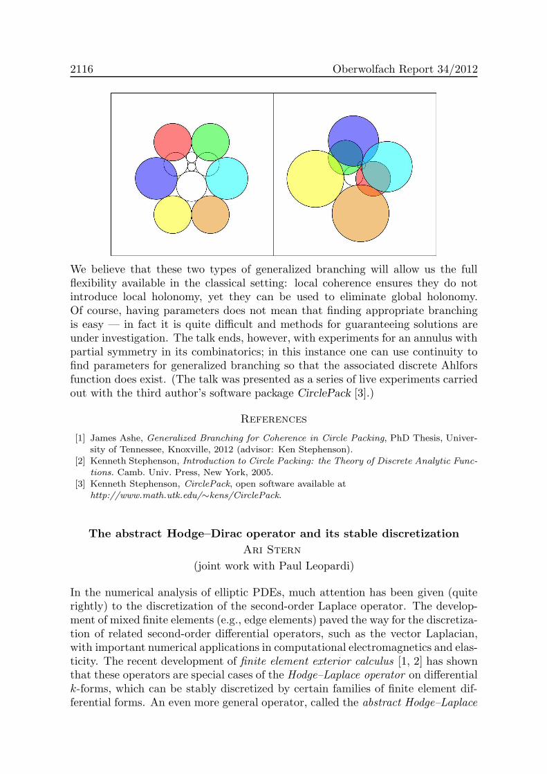
2116 Oberwolfach Report 34/2012
We believe that these two types of generalized branching will allow us the fullflexibility available in the classical setting: local coherence ensures they do notintroduce local holonomy, yet they can be used to eliminate global holonomy.Of course, having parameters does not mean that finding appropriate branchingis easy — in fact it is quite difficult and methods for guaranteeing solutions areunder investigation. The talk ends, however, with experiments for an annulus withpartial symmetry in its combinatorics; in this instance one can use continuity tofind parameters for generalized branching so that the associated discrete Ahlforsfunction does exist. (The talk was presented as a series of live experiments carriedout with the third author’s software package CirclePack [3].)
References
[1] James Ashe, Generalized Branching for Coherence in Circle Packing, PhD Thesis, Univer-sity of Tennessee, Knoxville, 2012 (advisor: Ken Stephenson).
[2] Kenneth Stephenson, Introduction to Circle Packing: the Theory of Discrete Analytic Func-tions. Camb. Univ. Press, New York, 2005.
[3] Kenneth Stephenson, CirclePack, open software available athttp://www.math.utk.edu/∼kens/CirclePack.
The abstract Hodge–Dirac operator and its stable discretization
Ari Stern
(joint work with Paul Leopardi)
In the numerical analysis of elliptic PDEs, much attention has been given (quiterightly) to the discretization of the second-order Laplace operator. The develop-ment of mixed finite elements (e.g., edge elements) paved the way for the discretiza-tion of related second-order differential operators, such as the vector Laplacian,with important numerical applications in computational electromagnetics and elas-ticity. The recent development of finite element exterior calculus [1, 2] has shownthat these operators are special cases of the Hodge–Laplace operator on differentialk-forms, which can be stably discretized by certain families of finite element dif-ferential forms. An even more general operator, called the abstract Hodge–Laplace

Discrete Differential Geometry 2117
operator, includes both the aforementioned Hodge–Laplace operator on k-forms,as well as other operators that arise, for example, in elasticity.
By comparison, discrete Dirac operators have received little attention from theperspective of numerical PDEs—despite being, in many ways, just as fundamentalas the widely-studied Laplace operators discussed above. Informally, a Dirac oper-ator is a square root of some Laplace operator, and is therefore a first-order (ratherthan second-order) differential operator. Dirac-type operators arise both in anal-ysis [11] and in differential geometry [14], in addition to their well-known, epony-mous origins in quantum mechanics [10]. The study of these first-order operatorsis also associated with a number of celebrated theorems, including the Atiyah–Singer index theorem [3], Witten’s proof of the positive energy theorem [17], andthe solution of the Kato square root problem [4]. Clifford analysis is the study ofDirac operators in various settings, including on smooth manifolds [8, 7].
Recently, there has been growing interest in developing a theory of discreteClifford analysis, based on lattice discretizations of Dirac operators [13, 12, 6]. Inmany respects, this work resembles the various lattice approaches to discretizingexterior calculus [9, 15, 5], particularly in the use of primal-dual mesh pairs. Theseapproaches are closer in spirit to finite difference methods than to finite elementmethods, in that they focus more on the degrees of freedom themselves than onbasis functions and interpolants. Consequently, these methods tend to be lessamenable to stability and convergence analysis, or to higher-order discretizations,compared with finite element exterior calculus. However, scant attention has beengiven to the possibility of using a mixed finite element approach to discretize Diracoperators and their associated first-order PDEs.
This talk reports on new work [16] which aims to fill this gap. We beginby devloping abstract Dirac operators and Hodge theory in terms of nilpotentoperators on Hilbert spaces, following the approach of [4], and introducing a mixedvariational problem associated to the Dirac operator. Next, we prove stabilityestimates, which establish well-posedness for both the continuous and discretevariational problems, as well as convergence estimates, given certain conditions onthe discretization. These discretization conditions correspond precisely to similarconditions in finite element exterior calculus, and consequently, we obtain stabilityand convergence for the well-studied Pr and P−
r finite element families of piecewise-polynomial differential forms. Finally, we show that many of the key estimates infinite element exterior calculus, which apply to discrete Laplace operators, can berecovered as corollaries of our estimates for discrete Dirac operators.
References
[1] D. N. Arnold, R. S. Falk, and R. Winther, Finite element exterior calculus, homologicaltechniques, and applications. Acta Numer. 15 (2006), 1–155.
[2] D. N. Arnold, R. S. Falk, and R. Winther, Finite element exterior calculus: from Hodgetheory to numerical stability. Bull. Amer. Math. Soc. (N.S.) 47 (2010), 281–354.
[3] M. F. Atiyah and I. M. Singer, The index of elliptic operators on compact manifolds, Bull.Amer. Math. Soc. 69 (1963), 422–433.

2118 Oberwolfach Report 34/2012
[4] A. Axelsson, S. Keith, and A. McIntosh, Quadratic estimates and functional calculi ofperturbed Dirac operators, Invent. Math. 163 (2006), 455–497.
[5] P. B. Bochev and J. M. Hyman, Principles of mimetic discretizations of differential opera-tors. In: D. N. Arnold et al., Compatible spatial discretizations. IMA Vol. Math. Appl. 142,Springer, New York 2006, 89–119.
[6] F. Brackx, H. De Schepper, F. Sommen, and L. Van de Voorde, Discrete Clifford analysis:a germ of function theory. In: I. Sabadini and M. Shapiro and F. Sommen, Hypercomplexanalysis. Trends Math., Birkhauser Verlag, Basel 2009, 37–53.
[7] J. Cnops, An introduction to Dirac operators on manifolds. Progress in MathematicalPhysics 24, Birkhauser Boston Inc., Boston, MA, 2002.
[8] R. Delanghe, Clifford analysis: history and perspective. Comput. Methods Funct. Theory 1
(2001), 107–153.[9] M. Desbrun, A. N. Hirani, M. Leok, and J. E. Marsden, Discrete exterior calculus. Preprint
2005.[10] P. A. M. Dirac, The quantum theory of the electron. Proc. R. Soc. Lond. A 117 (1928),
610–624.[11] M. G. Eastwood and J. Ryan, Aspects of Dirac operators in analysis. Milan J. Math. 75
(2007), 91–116.[12] N. Faustino, Discrete Clifford analysis. Ph.D. thesis, Universidade de Aveiro 2009.[13] N. Faustino, U. Kahler, and F. Sommen, Discrete Dirac operators in Clifford analysis. Adv.
Appl. Clifford Algebr. 17 (2007), 451–467.[14] T. Friedrich, Dirac operators in Riemannian geometry.Graduate Studies in Mathematics 25,
AMS, Providence, RI, 2000. Translated from the 1997 german original by Andreas Nestke.[15] J. Harrison, Ravello lecture notes on geometric calculus—Part I. Preprint 2005.[16] P. Leopardi and A. Stern, The abstract Hodge–Dirac operator and its stable discretization.
In preparation.[17] E. Witten, A new proof of the positive energy theorem. Comm. Math. Phys. 80 (1981),
381–402.
Lifting Spherical Cone Metrics
John M. Sullivan
Let Mdκ denote the (simply connected) “model” d-dimensional space of constant
curvature κ. (That is, spherical, euclidean, or hyperbolic space, depending on thesign of κ.) A cone metric on a (compact) d-dimensional pseudomanifold (withbackground curvature κ) is obtained by gluing (finitely many) simplices from Md
κ
together along isometries of their facets. Away from the (d− 2)-skeleton this givesa smooth metric of constant curvature. Around each face of codimension 2 wehave some cone angle α > 0; the angle defect 2π − α is a measure of curvature.In particular, the cone metric forms an Alexandrov space of curvature boundedbelow by κ if and only if all cone angles satisfy α ≤ 2π. (Similarly, the metric hascurvature bounded above by κ if and only if α ≥ 2π holds everywhere.)
For d = 2, a cone surface has a constant curvature metric away from finitelymany cone points. Each cone point contributes an atom 2π−α of Gauss curvatureand the Gauss–Bonnet formula holds in the form 2πχ = κA+
∑(2π − α), where
A is the area of the surface and the sum is over all cone points.For d = 3, the singular locus is an embedded graph with “straight” edges, each
with some constant cone angle α. Given an embedded graph in a 3-manifold onecan ask which cone metrics exist: for which values of κ and which assigments of

Discrete Differential Geometry 2119
α to each edge is there a corresponding cone metric? The rigidity question asks:when is the cone metric uniquely determined by this data? Even if the metric is notrigid, is the volume – and the length of the singular edges – uniquely determined?
We focus on the case of a link L = L1 ∪ · · · ∪ Lk of k components in S3. Theidea of studying cone metrics basically comes from Thurston, who showed that“most” links are hyperbolic in the sense that for small cone angles αi around thecomponents Li there is a hyperbolic (κ = −1) metric; in the limit αi → 0 we get acomplete hyperbolic metric on S3rL. (This metric is unique by Mostow rigidity.)
A standard example, illustrated nicely for instance in the 1991 video Not Knotfrom the Geometry Center, is the Borromean rings, taken with equal cone anglesα on all three components. For π < α < 2π there is a spherical cone metric.(As α → 2π the three singular axes limit to three orthogonally intersecting greatcircles in the equator of the round 3-sphere. It is known that the Borromean ringscannot be built from three round circles in S3 but of course we can come arbitrarilyclose.) For α = π we get a euclidean cone metric – the quotient of E3 by 2-foldrotations around the (non-intersecting, axis-parallel) lines of the primitive cubicrod packing [6]. (Equivalently, the 2-fold cover of S3 branched over the Borromeanrings is a 3-torus admitting a euclidean metric.) For 0 < α < π we get a hyperboliccone metric (in particular, for α = π/n this corresponds to a hyperbolic metric onan n-fold branched covering), and in the limit α→ 0 we get the hyperbolic metricon the link complement.
A d-orbifold is a space locally modeled on Rd/Γ for some finite point group Γ.Examples include quotients of Md
κ by any discrete group of isometries – theseinherit “smooth” orbifold metrics, meaning cone metrics with cone angles α =2π/n along the rotation axes of the orbifold.
Thurston used 2-orbifolds as base spaces for Seifert fibrations. These consistof some underlying surface with cone points (those of order n corresponding toΓ = Cn) and mirror boundaries (Γ = D1), which are straight except for coners(Γ = Dn). To compute the orbifold Euler characteristic χo (which is multiplicativeeven for branched covers) we start with the Euler characteristic of the underlyingsurface with boundary, and then subtract 1− 1/n for each n-fold cone point (andhalf that much for each mirror corner).
It is known that every 2-orbifold with χo < 0 admits a hyperbolic metric, i.e.,is a global quotient of H2. Similarly there are only 17 orbifolds with χo = 0,corresponding to the wallpaper groups and thus having euclidean metrics. Forχo > 0 we of course have orbifolds corresponding to the finite subgroups of O3
(the seven polyhedral groups and the seven infinite families of axial groups). Butthere are also the so-called “bad” orbifolds: spheres with two cone points of orders1 ≤ p < q (along with their quotients, disks with two corners of orders 1 ≤ p < q ontheir mirror boundary). These are the base spaces for the (p, q)-Seifert fibrations ofS3 by (p, q)-torus knots, but do not have spherical metrics. (There is no spherical
cone metric on S2 with just two unequal cone points, cf. [5].)Much of the interest in rigidity of cone metrics in three dimensions has been
related to the proofs by Cooper/Hodgson/Kerckhoff and by Boileau/Leeb/Porti

2120 Oberwolfach Report 34/2012
of Thurston’s orbifold geometrization conjecture. In an orbifold metric the coneangles satisfy α ≤ π and many known results are restricted to this range (but seee.g. [2]); we are instead particularly interested in spherical cone metrics with largecone angles.
Given a triangulation of S3 in which no edge has valence more than 5 – a com-puter enumeration with Frank Lutz shows there are exactly 4761 such simplicialcomplexes – we can give each tetrahedron the shape of one from the 600-cell:spherical regular with dihedral angles 2π/5 and edge lengths π/5. The cone anglearound an edge of valence v is then 2πv/5. We get a spherical cone metric ofcurvature bounded below by 1 in the sense of Alexandrov, leading immediately todiameter and volume bounds. In an ongoing project with Florian Frick, we havefocused first on the family whose cone axes (formed by the edges of valence lessthan 5) are unbranched, forming a link. We have found that most of these areSeifert-fibered, arising as lifts of spherical cone metrics on 2-orbifolds, in the sensewe now explain. (The Borromean rings also arise, as do certain graph manifolds.)
Recall that with the exception of hyperbolic and Sol geometries, the remainingsix Thurston geometries are those of Seifert fibered spaces, distinguished by thecurvature κ of the base and the curvature τ of the bundle [9]. Untwisted bundles(τ = 0) give the geometries M2
κ × R; twisted bundles (τ 6= 0) give the Berger
metrics on S3 if κ > 0; Nil or Heisenberg geometry if κ = 0; and SL(2,R) if κ < 0.We want to consider such twisted bundles over an aribtrary metric base. That
is, we’re interested in a Killing submersion from a 3-manifold to a surface, i.e., asubmersion where the unit vertical vector field Z is a Killing field, an infinitesimalisometry. The fundamental equations for Riemannian submersions are due toO’Neill [7]. Given a metric disk D with Gauss curvature function κ, and a Killingsubmersion from M = D × R, suppose that X and Y = JX = X × Z areorthonormal horizontal vector fields. Then ∇XZ = τY for some function τ on Mcalled the bundle curvature, and we find 〈[X,Y ], Z〉 = 2τ . The sectional curvaturesrange from κ− 3τ2 for the horizontal plane to τ2 for any vertical plane, cf. [1].
Suppose we start with a metric on D with κ ≥ 1, then scale down by a factorof two so that κ ≥ 4. Taking τ ≡ 1, the resulting metric on M has all sectionalcurvatures at least 1. Suppose γ is a closed curve enclosing areaA (before rescaling)in the base D. If we lift it to a horizontal curve in M , this lift fails to close and itsvertical holonomy is exactly A/2 (twice the rescaled area, since [X,Y ] = 2Z+ · · · ).Thus if we want to glue two such metrics together to get a bundle over S2, we needto take a quotient in the fiber direction, giving circles of some length ℓ. If the totalbase area is A, then to get the holonomy to match, we need A/2 = eℓ where e ∈ Z
will be the Euler class of the bundle. That is, to get S3 with the Hopf fibrationwe take e = 1 and ℓ = A/2. (For e > 1 we get the quotient of this by an e-foldHopf rotation, giving the lens space L(e, 1).)
Consider the case where the base is a spherical cone metric with k cone points ofcone angles αi. Then Gauss–Bonnet says A = 4π−∑
(2π−αi) = 2π(2−k)+∑αi.
Since the fiber length is ℓ = A/2 and the projected area is A/4 we find the volumeof the 3-sphere is V = A2/8. Now consider what happens when we change the αi.

Discrete Differential Geometry 2121
We obtain 2 dV = AdA/2 = ℓ∑dαi, which of course is the well-known Schlafli
formula.There are 17 (not necessarily simplicial) trianguations of S2 with valence up
to 5; giving their triangles the geometry of those in the icosahedron (with areaπ/5) we get 17 interesting spherical cone metrics on S2. Each one Hopf-lifts togive a cone metric on S3 and indeed these come from triangulations in our family.The lift of an example with f -vector (k + 2, 3k, 2k) has vertical length k π/5 andf -vector
(k(k+2), k(7k−2), 12k2, 6k2
). The lift of the icosahedron is the 600-cell;
the lift of the tetrahedron has 8 edges of valence 3 forming a 4-component Hopflink.
Now suppose we are given 1 ≤ p < q relatively prime and a spherical cone metricon S2 with one cone point of angle β ≤ 2π/p, a second of angle γ ≤ 2π/q and kfurther ones of angles αi. We view this as a spherical cone metric on the “bad”pq-orbifold. This we can lift along the (p, q)-Seifert fibration of S3 to give a conemetric on S3. Considering the Euler class of the bundle in the orbifold sense [9],we can check that the vertical length must now be pqA/2 (where A again is basearea). The cone angles are pβ and qγ along the two singular fibers and αi along acollection of (p, q)-torus knots (i.e., along a (kp, kq)-torus link). This constructionaccounts for most of the remaining triangulations we have been studying.
Note that in the special case of torus links with equal cone angles along eachcomponent, the geometric parameters for these spherical cone metrics have beendetermined previously via quite different methods [3]; see also [8, 4].
References
[1] J.M. Espinar, I.S. de Oliveira, Locally convex surfaces immersed in a Killing submersion.arXiv:1002.1329v1 (2010).
[2] I. Izmestiev, Examples of infinitesimally flexible 3-dimensional hyperbolic cone-manifolds.J. Math. Soc. Japan 63 (2011), 581–598.
[3] A.A. Kolpakov, Addendum to “Spherical structures on torus knots and links”, preprint(2011), arXiv:1101.1620v2.
[4] A.A. Kolpakov, A.D. Mednykh, Spherical structures on torus knots and links, Sib. Math.J. 50 (2009), 856–866
[5] F. Luo, G. Tian, Liouville equation and spherical convex polytopes. Proc. Amer. Math. Soc.116 (1992), 1119–1129.
[6] M. O’Keeffe, S. Andersson, Rod packings and crystal chemistry. Acta Cryst. A 33 (1977),914–923.
[7] B. O’Neill, The fundamental equations of a submersion. Michigan Math. J. 13 (1966), 459–469.
[8] J. Porti, Spherical cone structures on 2-bridge knots and links, Kobe J. Math. 21 (2004),61–70.
[9] P. Scott, The geometries of 3-manifolds. Bull. London Math. Soc. 15 (1983), 401–487.

2122 Oberwolfach Report 34/2012
Spherical geometry and integrable systems
Yuri B. Suris
(joint work with Matteo Petrera)
Nowadays, it is well accepted that geometry provides us with a wealth of importantinstances of integrable systems. In the present work, it is demonstrated that thecosine law for spherical simplices [7] defines integrable systems in several senses.
For a spherical triangle with the vertices v1, v2, v3 ∈ S2, with the sides ℓij
(connecting vi and vj) and the inner angles αij (opposite to ℓij), the cosine lawreads as follows:
(1) cos ℓij =cosαij + cosαik cosαjk
sinαik sinαjk.
Here (i, j, k) stands for an arbitrary permutation of (1, 2, 3). Putting xij = cosαij
and yij = cos ℓij , equation (1) is written in the algebraic form:
(2) yij =xij + xikxjk√1− x2ik
√1− x2jk
.
First interpretation of the spherical cosine law as an integrable system.In this interpretation, the quantities xij are combinatorially assigned to the three 2-faces of a 3-dimensional cube parallel to the coordinate planes ij, and the quantitiesyij = Tkxij to the three opposite 2-faces, cf. Fig. 1. Here, Tk stands for the unitshift in the k-th coordinate direction. In the terminology of [1], we consider a
x12
x23
x137→
y12
y23
y13
Figure 1. A map on an elementary 3D cube with fields assignedto 2-faces. We interpret yij as Tkxij , the shift of xij in the coor-dinate direction k.
3D system with fields assigned to elementary squares. This 3D system can becalled the symmetric discrete Darboux system, since it is a special case (symmetricreduction) xij = xji of the general discrete Darboux system, given by
(3) Tkxij =xij + xikxkj√
1− xikxki√1− xkjxjk
.
System (3) is well known in the theory of discrete integrable systems of geometricorigin. It describes the so called rotation coefficients of discrete conjugate nets

Discrete Differential Geometry 2123
f : Z3 → RPn, i.e., nets with planar elementary quadrilaterals, see [1, p. 42]. It
seems to have appeared for the first time in [4, eq. (7.20)]. Its symmetric reductionxij = xji is used for the description of the so called symmetric conjugate nets anddiscrete Egorov nets, see [2]. The symmetric discrete Darboux system is a closerelative of the discrete CKP system, see [6]. Thus, symmetric discrete Darbouxsystem admits an novel interpretation in terms of spherical triangles. Recall [1]that integrability of discrete 3D systems is synonymous with their 4D consistency.
Theorem 3. Symmetric discrete Darboux system is 4D consistent.
Our new interpretation leads also to a new proof of this (previously known)result. It consists in considering various geometric quantities within a sphericaltetrahedron, which combinatorially corresponds to a 4D cube.
Second interpretation of the spherical cosine law as an integrable sys-tem. In the second interpretation, we consider the dynamical system generatedby (iterations) of map (2) between open subsets of R3. It can be considered as atime discretization of the famous Euler top, described by the following system ofdifferential equations:
(4) xij = xikxjk .
The latter system is integrable in the Liouville-Arnold sense, is bi-Hamiltonian andadmits integrals of motion Ii = x2ij−x2ik, two of which are functionally independent.Discretization (2) of the Euler top turns out to inherit integrability.
Theorem 4. The map (2) is bi-Hamiltonian and admits integrals of motion
(5) Ei =1− x2ik1− x2ij
,
two of which are functionally independent. It has an invariant volume form
(6) ω =dx12 ∧ dx13 ∧ dx23
ϕ(x),
where ϕ(x) is any of the functions (1− x2ij)2.
Integrals of motion (5) express nothing but the sine law for spherical trian-gles. An unpleasant non-algebraic nature of discretization (2) is cured in a ratherunexpected way.
Theorem 5. On the subset of R3 where the second iterate of map (2) is defined,this second iterate is a birational map x 7→ x given by the (unique) solutions ofthe following system of equations:
(7) xij − xij = xikxjk + xikxjk,
which constitute the Hirota-Kimura discretization of the Euler top [3], [5].

2124 Oberwolfach Report 34/2012
Cosine law for spherical tetrahedra as an integrable system. Similarly tothe case of spherical triangles, we can consider a dynamical system generated bythe map x 7→ y between open subsets of R6, where xij = cosαij , yij = cos ℓij , andαij and ℓij are (opposite) dihedral angles and edges, respectively, of a sphericaltetrahedron. This map is given again by the corresponding cosine law. It can beconsidered as a time discretization of the following system of ordinary differentialequations:
(8) xij = xikxjk + ximxjm.
Here (i, j, k,m) stands for an arbitrary permutation of (1, 2, 3, 4). This 6-dimensionalsystem turns out to consist of two linearly coupled copies of the Euler top. As aconsequence, equations (8) are integrable in the Liouville-Arnold sense, with fourindependent integrals of motion which can be chosen as
x212 + x234 − x213 − x224, x213 + x224 − x223 − x214,
x12x34 − x13x24, x13x24 − x23x14.
Theorem 6. The map x 7→ y defined by the cosine law for spherical tetrahedraadmits four independent integrals of motion
(9)(1 − x213)(1 − x224)
(1 − x212)(1 − x234),
(1− x223)(1− x214)
(1− x212)(1− x234),
(10)x12x34 − x13x24√(1 − x212)(1 − x234)
,x13x24 − x23x14√(1− x212)(1− x234)
.
It has an invariant volume form
(11) ω =dx12 ∧ dx13 ∧ dx23 ∧ dx14 ∧ dx24 ∧ dx34
ϕ(x),
where ϕ(x) is any of the functions (1− x2ij)5/2(1− x2km)5/2.
Again, integrals of motion express nothing but the sine law for spherical tetra-hedra.
References
[1] A.I. Bobenko, Yu.B. Suris, Discrete Differential Geometry. Integrable Structure. GraduateStudies in Mathematics 98, AMS, 2008.
[2] A. Doliwa, The C-(symmetric) quadrilateral lattice, its transformations and the algebro-geometric construction, J. Geom. Phys. 60 (2010), 690–707.
[3] R. Hirota, K. Kimura, Discretization of the Euler top. J. Phys. Soc. Japan, 69 (2000),627-630.
[4] B. G. Konopelchenko, W. K. Schief, Three-dimensional integrable lattices in Euclideanspaces: conjugacy and orthogonality. Proc. R. Soc. Lond. A 454 (1998), 3075–3104.
[5] M. Petrera, Yu.B. Suris, On the Hamiltonian structure of Hirota-Kimura discretization ofthe Euler top. Math. Nachr. 283 (2011), 1654-1663.
[6] W. K. Schief, Lattice Geometry of the Discrete Darboux, KP, BKP and CKP Equations.Menelaus’ and Carnot’s Theorems. J. Nonlin. Math. Phys. 10 (2003), 194–208.
[7] E.B. Vinberg (Ed.), Geometry II. Encyclopaedia of Mathematical Sciences 29, Springer-Verlag 1993.

Discrete Differential Geometry 2125
Higher pentagram maps, directed weighted networks, and clusteralgebras
Serge Tabachnikov
This is a report on a joint work in progress with M. Gekhtman, M. Shapiro andA. Vainstein [3].
Given a convex n-gon P in the projective plane, let T (P ) be the convex hullof the intersection points of consecutive shortest diagonals of P . The map Tcommutes with projective transformations and hence defines a map on the modulispace of projective equivalence classes of polygons. This map was defined by R.Schwartz [13]; it is called the pentagram map. The pentagram map is also definedon a larger class of twisted polygons, that is, polygons with monodromy that is aprojective transformation.
The pentagram map has attracted much interest in the recent years; see [14,15, 9, 10, 16] for a sampler. The main result is that it is a discrete completelyintegrable system. It was observed by M. Glick [4] that the pentagram map isclosely related with the emerging theory of cluster algebras. The goal of ourwork was to extend the pentagram map to other dimensions and to establish itscomplete integrability using the techniques of weighted directed networks [11, 2].Let us mention different approaches to higher dimensional pentagram maps andrelated systems, developed in [5], in [6, 7], and in [8].
Glick interpreted the pentagram map is a sequence of mutations associatedwith a special homogeneous bipartite quiver. We generalized Glick’s quiver toa family of quivers embedded in the torus. The dual graph of this quiver is acertain weighted directed network on the torus, and the mutations are realized as asequence of Postnikov moves on this network, followed by a gauge transformationsof the respective variables. This results in the family of rational maps Tk:
x∗i = xi−r−1xi+r + yi+r
xi−r−1 + yi−r−1, y∗i = yi−r
xi+r+1 + yi+r+1
xi−r + yi−r, k even,
x∗i = xi−r−2xi+r + yi+r
xi−r−2 + yi−r−2, y∗i = yi−r−1
xi+r+1 + yi+r+1
xi−r−1 + yi−r−1, k odd.
where r = [k/2]− 1, k ≥ 2. The map T3 is the pentagram map.The maps Tk are completely integrable. All the ingredients needed for complete
integrability (invariant Poisson bracket, integrals in involution, zero curvature rep-resentation) are provided by the “technology” of weighted directed networks, asdescribed in [2]. Specifically, Tk has an invariant Poisson bracket (for n ≥ 2k− 1):
xi, xi+l = −xixi+l, 1 ≤ l ≤ k − 2; yi, yi+l = −yiyi+l, 1 ≤ l ≤ k − 1;
yi, xi+l = −yixi+l, 1 ≤ l ≤ k − 1; yi, xi−l = yixi−l, 0 ≤ l ≤ k − 2.
The functions∏xi and
∏yi are Casimir. If n is even and k is odd, one has four
Casimir functions:∏
i even
xi,∏
i odd
xi,∏
i even
yi,∏
i odd
yi.

2126 Oberwolfach Report 34/2012
The integrals come from the boundary measurement matrix of the respectivenetwork. Namely, for k ≥ 3, let
Li =
0 0 0 . . . xi xi + yiλ 0 0 . . . 0 00 1 0 . . . 0 00 0 1 . . . 0 0. . . . . . . . . . . . . . . . . .0 0 0 . . . 1 1
,
and for k = 2,
Li =
(λxi xi + yiλ 1
).
The boundary measurement matrix is M(λ) = L1 · · ·Ln. The characteristic poly-nomial
det(M(λ) − z) =∑
Iij(x, y)ziλj .
is Tk-invariant, and the integrals Iij are in involution.A geometric interpretation of the maps Tk is as follows.Let k ≥ 3, and denote by Pk,n the space of projective equivalence classes of
generic twisted n-gons in RPk−1. Let P 0k,n ⊂ Pk,n consist of the polygons with
the following property: for every i, the vertices Vi, Vi+1, Vi+k−1 and Vi+k spana projective plane. These are called corrugated polygons. The consecutive k −1-diagonals of a corrugated polygon intersect. The resulting polygon is againcorrugated. One gets a pentagram-like k − 1-diagonal map on P 0
k,n. For k = 3,this is the pentagram map.
Lift the vertices Vi of a corrugated polygon to vectors Vi in Rk so that thelinear recurrence holds
Vi+k = yi−1Vi + xiVi+1 + Vi+k−1,
where xi and yi are n-periodic sequences. These are coordinates in P 0k,n. In these
coordinates, the map is identified with Tk.The geometric interpretation is different for k = 2. Consider the space Sn of
pairs of twisted n-gons (S−, S) in RP1 with the same monodromy. Consider theprojectively invariant projection φ to the (x, y)-space:
xi =(Si+1 − S−
i+2)(S−i − S−
i+1)
(S−i − Si+1)(S
−i+1 − S−
i+2)
yi =(S−
i+1 − Si+1)(S−i+2 − Si+2)(S
−i − S−
i+1)
(S−i+1 − Si+2)(S
−i − Si+1)(S
−i+1 − S−
i+2).
Then xi, yi are coordinates in Sn/PGL(2,R).Define a transformation (S−, S) 7→ (S, S+), where S+ is given by the following
local “leapfrog” rule: given points Si−1, S−i , Si, Si+1, the point S+
i is obtained by

Discrete Differential Geometry 2127
the reflection of S−i in Si in the projective metric on the segment [Si−1, Si+1]. The
projection φ conjugates this leapfrog map with with T2. In formulas:
1
S+i − Si
+1
S−i − Si
=1
Si+1 − Si+
1
Si−1 − Si,
or, equivalently,(S+
i − Si+1)(Si − S−i )(Si − Si−1)
(S+i − Si)(Si+1 − Si)(S
−i − Si−1)
= −1.
Over the field of complex numbers, these formulas can be interpreted as a circlepattern studied by O. Schramm [12]; see also [1].
References
[1] A. Bobenko, T. Hoffmann, Hexagonal circle patterns and integrable systems: patterns withconstant angles. Duke Math. J. 116 (2003), 525–566.
[2] M. Gekhtman, M. Shapiro, A. Vainshtein, Cluster algebras and Poisson geometry. Amer.Math. Soc., Providence, RI, 2010.
[3] M. Gekhtman, M. Shapiro, S. Tabachnikov, A. Vainshtein, Higher pentagram maps, weighteddirected networks, and cluster dynamics. Electron. Res. Announc. Math. Sci. 19 (2012), 1–17.
[4] M. Glick, The pentagram map and Y -patterns. Adv. Math. 227 (2011), 1019–1045.[5] A. Goncharov, R. Kenyon, Dimers and cluster integrable systems. arXiv:1107.5588.[6] B. Khesin, F. Soloviev, Integrability of higher pentagram maps. arXiv:1204.0756.[7] B. Khesin, F. Soloviev, The Pentagram map in higher dimensions and KdV flows.
arXiv:1205.3744.[8] A. Marshakov, Lie groups, cluster variables and integrable systems. arXiv:1207.1869.[9] V. Ovsienko, R. Schwartz, S. Tabachnikov, The Pentagram map: a discrete integrable sys-
tem. Commun. Math. Phys. 299 (2010), 409–446.[10] V. Ovsienko, R. Schwartz, S. Tabachnikov, Liouville-Arnold integrability of the pentagram
map on closed polygons. arXiv:1110.0472.[11] A. Postnikov, Total positivity, Grassmannians, and networks. arXiv:math.CO/0609764.
[12] O. Schramm, Circle patterns with the combinatorics of the square grid. Duke Math. J. 86(1997), 347–389.
[13] R. Schwartz, The pentagram map. Experiment. Math. 1 (1992), 71–81.[14] R. Schwartz, The pentagram map is recurrent. Experiment. Math. 10 (2001), 519–528.[15] R. Schwartz, Discrete monodromy, pentagrams, and the method of condensation. J. Fixed
Point Theory Appl. 3 (2008), 379-409.[16] F. Soloviev, Integrability of the Pentagram Map. arXiv:1106.3950.
Design of Self-supporting Surfaces
Etienne Vouga
(joint work with Mathias Hobinger, Johannes Wallner, Helmut Pottmann)
Vaulted masonry structures are among the simplest and at the same time mostelegant solutions for creating curved shapes in building construction. For thisreason they have been an object of interest since antiquity, and continue to be anactive topic of research today.
We study the combined geometry and statics of self-supporting masonry, anddevelop a tool for the interactive modeling of freeform self-supporting structures.

2128 Oberwolfach Report 34/2012
Here “self-supporting” means that the structure is in static equilibrium under itsown weight. This analysis is based on the following classic [8] assumptions: 1)masonry has no tensile strength, and infinite compressive strength; and 2) (TheSafe Theorem) if a system of forces can be found which is in equilibrium with theload on the structure and which is contained within the masonry envelope thenthe structure will also carry the loads. A more detailed account of what follows isavailable in [12].
1. Modeling Self-supporting Surfaces
We model masonry as a surface given by a height field s(x, y) and assume aload density F (x, y) over the top view. The surface is in static equilibrium whenthere exists a field of symmetric positive-definite matrices M(x, y) satisfying
div(M∇s) = F, divM = 0,
where the divergence operator acts on the columns of a matrix [5, 6].We discretize self-supporting surfaces as a thrust network [2]: a mesh S =
(V,E, F ) with loads FiAi on vertices vi. Stresses are carried by the edges of themesh: the force exerted on vi by the edge connecting vi,vj is given by
wij(vj − vi), where wij = wji ≥ 0.
The nonnegativity of the individual weights expresses the compressive nature offorces. Equilibrium at vertices is then given by balance of stresses and loads.
Invoking the safe theorem, a masonry structure is self-supporting if we canfind a thrust network with compressive forces which is entirely contained withinthe structure. Finding a self-supporting surface near one that is not amountsto solving for a simultaneous solution in vi and wij . We develop an interactivetool for efficiently finding such a solution: we iteratively alternate between fixingpositions and solving for weights wij that best minimize the least-square errorin equilibrium, and fixing the weights and solving for displacements to vi thatlikewise decrease the error. To prevent the surface from drifting too far away fromthe input shape specified by the user, we regularize the latter step by introducingterms to the objective that penalize total and normal displacement of the vertices.
2. Geometrization of Equilibrium
In both the continuous and discrete settings, static equilibrium of the surfacecan be formulated in terms of several geometric structures, each with rich connec-tions to discrete differential geometry:
2.1. Stress Laplacian. The smooth equilibrium equations can be written interms of an elliptic Laplace-like operator ∆M = divM∇. Likewise, the weightswij define a graph Laplacian ∆w on the top view (projection onto the plane) ofthe thrust network. This discrete Laplacian is perfect in the sense of [13].

Discrete Differential Geometry 2129
2.2. Airy Stress Potential. Symmetry of M together with divM = 0 are inte-grability conditions on the components of M , so that M is locally determined bythe Hessian of a convex real-valued function φ (the Airy stress potential) [7].
Horizontal equilibrium of the discrete thrust network implies existence of anorthogonal dual to the top view S ′, the reciprocal diagram [2]. From this dualwe construct a convex “Airy stress polyhedron” Φ with planar faces and top viewS ′ [1]: the gradient jump between two adjacent faces of the stress polyhedron isequal to the edge vector on the reciprocal diagram dual to their shared edge. (If S ′
is not simply connected, Φ exists locally.) This Airy stress polyhedron can also beconstructed as the finite element discretization of the continuous Airy function [5].
Formulating equilibrium in terms of the Airy stress potential allows us to findPQ remeshings of self-supporting quad meshes where naively introducing a pla-narity constraint to the optimization fails: the top view of a PQ remeshing mustsimultaneously admit a PQ remeshing of the stress surface. This can be assuredby finding the unique curve networks simultaneously conjugate on φ and s [9],
given by tracing the eigenvectors of ∇2φ−1∇2s.
2.3. Isotropic Curvature Relations. Equilibrium of the surface can be phrasedin terms of purely geometric curvature measures of s and φ by passing to dualisotropic geometry: 2KφH
rels = F , where Kφ is dual-isotropic Gaussian curvature
(with respect to the Maxwell paraboloid) and Hrels is dual-isotropic relative mean
curvature. An identical relationship, in terms of mixed-area formulas for discretecurvature [11, 3, 10], holds for discrete thrust networks. As a consequence ofthis relationship, we can construct special families of self-supporting surfaces, byadding to the dual of a Koenigs mesh [4] a multiple of its Christoffel dual.
References
[1] Ash, P., Bolker, E., Crapo, H., and Whiteley, W., Convex polyhedra, Dirichlet tessellations,and spider webs. In: Shaping space (Northampton 1984). Birkhauser 1988, 231–250.
[2] Block, P., and Ochsendorf, J., Thrust network analysis: A new methodology for three-dimensional equilibrium. J. Int. Assoc. Shell and Spatial Structures 48 (2007), 167–173.
[3] Bobenko, A., Pottmann, H., and Wallner, J., A curvature theory for discrete surfaces basedon mesh parallelity. Math. Annalen 348 (2010), 1–24.
[4] Bobenko, A., and Suris, Yu., Discrete differential geometry: Integrable Structure. GraduateStudies in Math. 98, AMS 2008.
[5] Fraternali, F., A thrust network approach to the equilibrium problem of unreinforced ma-sonry vaults via polyhedral stress functions. Mechanics Res. Comm. 37 (2010), 198–204.
[6] Giaquinta, M., and Giusti, E., Researches on the equilibrium of masonry structures. Archive
for Rational Mechanics and Analysis 88 (1985), 359–392.[7] Green, A., and Zerna, W., Theoretical Elasticity. Dover 2002. Reprint of the 1968 edition.[8] Heyman, J., The stone skeleton. Int. J. Solids Structures 2 (1966), 249–279.[9] Liu, Y., Pottmann, H., Wallner, J., Yang, Y.-L., and Wang, W., Geometric modeling with
conical meshes and developable surfaces. ACM Trans. Graphics (Proc. SIGGRAPH) 25
(2006), 681–689.[10] Pottmann, H., and Liu, Y., Discrete surfaces in isotropic geometry. In: M. Sabin and J.
Winkler (Eds.), Mathematics of Surfaces XII, Springer 2007, 341–363.
2130 Oberwolfach Report 34/2012
[11] Pottmann, H., Liu, Y., Wallner, J., Bobenko, A., and Wang, W., Geometry of multi-layerfreeform structures for architecture. ACM Trans. Graphics (Proc. SIGGRAPH) 26 (2007),1–11.
[12] Vouga, E., Hobinger, M., Wallner, J., and Pottmann, H., Design of self-supporting surfaces.ACM Trans. Graphics (Proc. SIGGRAPH) 31 (2012).
[13] Wardetzky, M., Mathur, S., Kalberer, F., and Grinspun, E., Discrete Laplace operators: Nofree lunch. In: A. Belyaev and M. Garland (Eds.), Symposium on Geometry Processing.Eurographics Assoc. 2007, 33–37.
Open problems in Discrete Differential Geometry
Collected by Klaus Hildebrandt
Problem 1 (B. Benedetti). Let C be a convex simplicial complex. Is it true thatthe barycentric subdivision of C is shellable?
So far we can prove a weaker claim: if a complex is convex and d-dimensional,then after at most d+ 2 consecutive barycentric subdivisions it becomes shellable(see my preprint with Karim Adiprasito, arXiv:1202.6606).
Glossary: A simplicial complex is called convex if it has a geometric real-ization in some Rk that is convex. In other words, a convex complex is a lineartriangulation of some convex polytope. A triangulated ball B is called shellable ifits facets can be labeled 1, . . . , N , so that the subcomplex determined by the firsti facets is a ball (for each i ≤ N).
History: A connection between shellability and convexity has been knownsince 1852: The boundary of every convex polytope is shellable. (See e.g. Ziegler,Lectures on Polytopes.) In 1958 Mary E. Rudin found an unshellable subdivisionof a tetrahedron; so, not every convex complex is shellable. However, the firstbarycentric subdivision of Rudin’s ball is shellable.
Problem 2 (U. Brehm). For a given non-trivial isotopy type of knots (or links)find (approximate numerically) a 2-dimensional branched surface M (standardspine, possibly with 1-dimensional parts) of minimal area having the followingproperty: There exists a knot (or link) K ⊆ R
3 of the given isotopy type such that
(1) d(M,K) = 1(2) M is a deformation retract of R3\K.
Exercise: The following should be true and not difficult to show: There existsa pair (M,K) (as specified above) minimizing area(M) and such anM contains anopen dense subset consisting of pieces of minimal surfaces and points with distance1 from K.
Problem 3 (Dmitry Chelkak). Let Γ and Γ∗ be two dual planar graphs embeddedin the plane so that corresponding dual edges are orthogonal. In this setup, onecan naturally introduce discrete ∂ and ∂ operators acting on functions defined
on Λ = Γ ∪ Γ∗, and the (cotangent-weight) Laplacian ∆ = 4∂∗∂ = 4∂∗∂ which
(independently) acts on functions defined on Γ and Γ∗.

Discrete Differential Geometry 2131
Under some mild assumptions on Γ and Γ∗ (like “no big faces and no thinangles”) prove the following uniform asymptotics of the free Green’s function
G(u;u0) =1
2πlog |u− u0|+O(1), u, u0 ∈ Γ,
and the Cauchy kernel
K(v; z0) = O(|v − z0|−1), v ∈ Λ, z0 ∈ ♦ = Λ∗.
If Λ is a rhombic lattice (and Γ,Γ∗ are isoradial graphs), those asymptotics areknown with much higher precision, so the question is how to derive the weakerstatement in the more general setup, where no “integrability approach” is avail-able. If proven, the first result would yield most of the “discrete complex analysistoolbox” reported on this workshop, while the second, in particular, would implythe uniform Lipshitzness of discrete harmonic functions (which, as far as we know,remains annoyingly unknown in this case).
Problem 4 (Ivan Izmestiev). Let M be a metrically complete non-compact Eu-clidean surface with finitely many cone singularities of negative curvature. Is ittrue that for every point x ∈M there exists a geodesic ray starting from x, missingall singular points and escaping to infinity?
Motivation: Joseph O’Rourke posed at the last workshop the problem whethera point in the plane can be shaded by straight segment mirrors. By gluing togethertwo copies of the plane cut along those segments (the left side of each slit to theleft, the right to the right), one obtains a Euclidean cone-surface of the kind de-scribed above. A light-ray trajectory on the plane is a geodesic on the surface.Thus a positive answer to the question would imply that mirrors cannot shade apoint.
Problem 5 (Rick Kenyon). Let T1, T2 be two independent and uniformly randomtriangulations of an n-gon (without internal vertices). Glue these triangulationstogether along the boundary n-gon to form a triangulation (in the generalizedsense) of the 2-sphere. What is the typical or expected diameter of the resultinggraph (in the graph metric)? It is conjectured to be of order n1/4+o(1).
Problem 6 (Jurgen Richter-Gebert). This problem comes from characterizingwhen 10 points in the projective plane lie on a common cubic. In the formulationbelow it can be considered independent from this geometric interpretation. Toformulate the problem we first need a little preparation. We start by consideringthe following set of ordered triples
A := (0, 1, 2), (0, 3, 4), (0, 5, 6), (1, 3, 7), (2, 4, 7) ,(1, 5, 8), (2, 6, 8), (3, 5, 9), (4, 6, 9), (7, 8, 9)
The combinatorics of these triples comes from the triples of a Desargues configu-ration. For a permutation π ∈ S10 we denote the set of permuted ordered triplesby
π(A) := (π(i), π(j), π(k)) | (i, j, k) ∈ A

2132 Oberwolfach Report 34/2012
and the set of corresponding sets by
π(A) := π(i), π(j), π(k) | (i, j, k) ∈ ASince the automorphism group of Desargues configuration has order 120 the set
π(A) | π ∈ S10 contains 10!/5! = 30240 elements. Finally let X ⊂ S10 be acollection of permutations with
π(A) | π ∈ X = π(A) | π ∈ S10and |X | = 30240.
Now we consider 10 points p0, . . . , p9 in the projective plane presented by ho-mogeneous coordinates. The following is a fact (that is not too difficult to prove):The points p0, . . . , p9 are on a common conic if and only if
f :=∑
π∈X
sign(π) ·
∏
(i,j,k)∈π(A)
det(pi, pj , pk)
vanishesThe expression f is well defined since it turns out that for any two permutations
π1, π2 ∈ S10 with π1(A) = π2(A) we have
sign(π1) ·∏
(i,j,k)∈π1(A)
det(pi, pj , pk) = sign(π2) ·∏
(i,j,k)∈π2(A)
det(pi, pj, pk).
Question: Is there a proper subset X ′ ⊂ X such that
∑
π∈X′
sign(π) ·
∏
(i,j,k)∈π(A)
det(pi, pj , pk)
is a factor of f .
Problem 7 (Serge Tabachnikov). An equilateral plane n-gon V1V2 . . . Vn is calleda bicycle (n, k)-gon if, for all i, the quadrilateral ViVi+1Vi+kVi+k+1 is an isoscelestrapezoid: ViVi+k+1 is parallel to Vi+1Vi+k and |ViVi+k| = |Vi+1Vi+k+1| (here2 ≤ k ≤ n/2). In terms of the discrete Darboux transformation [3], a bicyclepolygon coincides with its Darboux image, up to a cyclic relabeling. A regularn-gon is a bicycle (n, k)-gon for all k.
The problem is to describe bicycle (n, k)-gons. In particular, for which pairs(n, k) is the regular polygon the only solution to the problem? For example, inthe following cases every bicycle (n, k)-gon is regular [4]:1) n arbitrary and k = 2;2) n odd and k = 3;3) k arbitrary and n = 2k + 1;4) k arbitrary and n = 3k.
On the other hand, for k odd and n even, there exists a 1-parameter familyof non-congruent bicycle (n, k)-gons. They are constructed by erecting medianperpendiculars of the same length to the sides of a regular n/2-gon; the resulting

Discrete Differential Geometry 2133
n-gon has dihedral symmetry so, for odd k, its k-diagonals are congruent. Onecan prove that every bicycle (4n, n)-gon is obtained this way.
A regular n-gon is infinitesimally flexible, as a bicycle (n, k)-gon, if and only if
tan(krπ
n
)tan
(πn
)= tan
(kπ
n
)tan
(rπ
n
)
for some 2 ≤ r ≤ n − 2 ([4]). This equation has the following solutions ([1]):assuming that r ≤ n/2, one has k+ r = n/2 and n|(k− 1)(r− 1). The solutions tothis equation that are not covered by the examples from the previous paragraphare second-order flexible but third-order rigid ([2]). Thus one conjectures thatthese examples are the only examples of bicycle (n, k)-gons with k < n/2 (bicycle(2n, n)-gons have a considerable flexibility).
The problem has a continuous version that justifies the terminology. The prob-lem is to describe pairs of closed plane curves, the rear and front bicycle tracks,such that one cannot tell which way the bicycle went; a pair of concentric circlesprovides a trivial example. This problem is equivalent to the 2-dimensional versionof Ulam’s problem: which uniform bodies float in equilibrium in all positions? See[4] and [5] and the references therein.
References
[1] R. Connelly, B. Csikos, Classification of first-order flexible regular bicycle polygons. StudiaSci. Math. Hungar. 46 (2009), 37–46.
[2] B. Csikos, On the rigidity of regular bicycle (n,k)-gons. Contrib. Discrete Math. 2 (2007),93–106.
[3] U. Pinkall, B. Springborn, S. Weißmann, A new doubly discrete analogue of smoke ring flowand the real time simulation of fluid flow. J. Phys. A 40 (2007), 12563–12576.
[4] S. Tabachnikov, Tire track geometry: variations on a theme. Israel J. Math. 151 (2006),1–28.
[5] F. Wegner, Three problems – one solution. http://www.tphys.uni-heidelberg.de/
~wegner/Fl2mvs/Movies.html
Reporter: Stefan W. von Deylen

2134 Oberwolfach Report 34/2012
Participants
Karim Adiprasito
Institut fur Mathematik I (WE 1)Freie Universitat BerlinArnimallee 214195 Berlin
Dr. Arseniy Akopyan
Dobrushin Mathematics LaboratoryInstitute for Problems of InformationTransmissionBolshoy Karetny per. 19127994 MOSCOWRUSSIAN FEDERATION
Prof. Dr. Marc Alexa
Fakultat f. Elektrotechnik u. InformatikTU BerlinEinsteinufer 1710587 Berlin
Dr. Bruno Benedetti
Matematiska InstitutionenKungl. Tekniska HogskolanLindstedtsvagen 2510044 STOCKHOLMSWEDEN
Prof. Dr. Alexander I. Bobenko
Institut fur MathematikFakultat II - Sekr. MA 8 - 3Technische Universitat BerlinStraße des 17. Juni 13610623 Berlin
Prof. Dr. Ulrich Brehm
Institut fur GeometrieTU Dresden01062 Dresden
Dr. Ulrike Bcking
Institut fur MathematikFakultat II - Sekr. MA 8 - 3Technische Universitat BerlinStraße des 17. Juni 13610623 Berlin
Cesar Ceballos
Fachbereich Mathematik & InformatikFreie Universitat BerlinArnimallee 614195 Berlin
Dr. Dmitry Chelkak
St. Petersburg Branch of SteklovMathematical Institute ofRussian Academy of ScienceFontanka 27191 023 ST. PETERSBURGRUSSIAN FEDERATION
Keenan Crane
Department of Computer ScienceCalifornia Institute of Technology1200 East California BoulevardPASADENA CA 91125UNITED STATES
Prof. Dr. Adam Doliwa
Department of Mathematics andComputer SciencesUniversity of Warmia & Mazuryul. Sloneczna 5410-710 OLSZTYNPOLAND
Andrew Furnas
Department of MathematicsBrown UniversityBox 1917PROVIDENCE, RI 02912UNITED STATES
Discrete Differential Geometry 2135
Dr. Alexander A. Gaifullin
Dept. of Geometry and TopologySteklov Mathematical InstituteGubkina Str. 8GSP-1 MOSCOW 119991RUSSIAN FEDERATION
Prof. Dr. Alexander B. Goncharov
Department of MathematicsYale UniversityBox 208 283NEW HAVEN, CT 06520UNITED STATES
Felix Gnther
Fachbereich MathematikTechnische Universitat BerlinStraße des 17. Juni 13610623 Berlin
Dr. Udo Hertrich-Jeromin
Department of Mathematical SciencesUniversity of BathClaverton DownBATH BA2 7AYUNITED KINGDOM
Klaus Hildebrandt
Fachbereich Mathematik & InformatikFreie Universitat BerlinArnimallee 614195 Berlin
Prof. Dr. Tim Hoffmann
Zentrum MathematikTU MunchenBoltzmannstr. 385748 Garching b. Munchen
Dr. Ivan Izmestiev
Fachbereich MathematikTU DarmstadtSchloßgartenstr. 764289 Darmstadt
Prof. Dr. Michael Joswig
Fachbereich MathematikTU DarmstadtDolivostr. 1564293 Darmstadt
Prof. Dr. Richard Kenyon
Department of MathematicsBrown UniversityBox 1917PROVIDENCE, RI 02912UNITED STATES
Felix J. Knppel
Institut fur MathematikMA 8 - 3Technische Universitat BerlinStraße des 17. Juni 13610623 Berlin
Dr. Christian Lessig
Department of Computing andMathematical SciencesCalifornia Institute of TechnologyPASADENA, CA 91125UNITED STATES
Dr. Yaron Lipman
Department of Computer Scienceand Applied MathematicsThe Weizmann Institute of ScienceP.O.Box 26REHOVOT 76100ISRAEL
Prof. Dr. Feng Luo
Department of MathematicsRutgers UniversityHill Center, Busch Campus110 Frelinghuysen RoadPISCATAWAY, NJ 08854-8019UNITED STATES

2136 Oberwolfach Report 34/2012
Prof. Dr. Christian Mercat
IREMUniversite de LyonBatiment Braconnier43 Bd. du 11 novembre 191869622 VILLEURBANNEFRANCE
Prof. Dr. Ulrich Pinkall
Institut fur MathematikTechnische Universitat BerlinSekr. MA 3-2Straße des 17. Juni 13610623 Berlin
Prof. Dr. Konrad Polthier
Institut fur MathematikFreie Universitat BerlinArnimallee 614195 Berlin
Prof. Dr. Jrgen Richter-Gebert
Zentrum MathematikTU MunchenBoltzmannstr. 385748 Garching b. Munchen
Prof. Dr. Igor Rivin
Department of MathematicsTemple UniversityTU 038-16PHILADELPHIA, PA 19122UNITED STATES
Dr. Thilo Rrig
Institut fur MathematikMA 8 - 3Technische Universitat BerlinStraße des 17. Juni 13610623 Berlin
Prof. Dr. Raman Sanyal
Institut fur Mathematik IFreie Universitat BerlinArnimallee 2-614195 Berlin
Prof. Dr. Wolfgang K. Schief
School of Mathematics & StatisticsThe University of SydneySYDNEY NSW 2052AUSTRALIA
Prof. Dr. Jean-Marc Schlenker
Institut de Mathematiques de ToulouseUniversite Paul Sabatier118, route de Narbonne31062 TOULOUSE Cedex 9FRANCE
Prof. Dr. Peter Schrder
Annenberg Center, CMSMC 305-16California Institute of Technology1200 E. California Blvd.PASADENA, CA 91125-5000UNITED STATES
Henrik Schumacher
Institut fur Numerischeund Angewandte MathematikUniversitat GottingenLotzestr. 16-1837083 Gottingen
Stefan Sechelmann
Institut fur MathematikFakultat II - Sekr. MA 8 - 3Technische Universitat BerlinStraße des 17. Juni 13610623 Berlin
Dr. Mikhail Skopenkov
The Institute for InformationTransmission Problems RASBuilding 1Bolshoy Karetny per. 19127994 MOSCOWRUSSIAN FEDERATION

Discrete Differential Geometry 2137
Prof. Dr. Olga Sorkine
Department of Computer ScienceETH Zurich, CNB G 106.2Universitatstr. 68092 ZURICHSWITZERLAND
Prof. Dr. Boris Springborn
Zentrum MathematikTechnische Universitat MunchenBoltzmannstr. 385747 Garching bei Munchen
Prof. Dr. Kenneth Stephenson
Department of MathematicsUniversity of Tennessee320 Ayres HallKNOXVILLE, TN 37996-1300UNITED STATES
Prof. Dr. Ari Stern
Department of MathematicsWashington University in St. LouisCampus Box 1146One Brookings DriveST. LOUIS, MO 63130-4899UNITED STATES
Prof. Dr. John M. Sullivan
Institut fur MathematikTechnische Universitat BerlinSekr. MA 3-2Straße des 17. Juni 13610623 Berlin
Prof. Dr. Yuri B. Suris
Fachbereich MathematikSekr. MA 7-2Technische Universitat BerlinStraße des 17. Juni 13510623 Berlin
Prof. Dr. Sergei Tabachnikov
Department of MathematicsPennsylvania State UniversityUNIVERSITY PARK, PA 16802UNITED STATES
Stefan W. von Deylen
Fachbereich Mathematik & InformatikFreie Universitat BerlinArnimallee 614195 Berlin
Prof. Dr. Etienne Vouga
Department of Computer ScienceColumbia UniversityNEW YORK NY 10027-7003UNITED STATES
Prof. Dr. Uli Wagner
Institut de Mathematiques de Geometrieet ApplicationsEPFL SB MATHGEOMMA-C1-533Station 81015 LAUSANNESWITZERLAND
Prof. Dr. Johannes Wallner
Institut fur GeometrieTU GrazKopernikusgasse 248010 GRAZAUSTRIA
Prof. Dr. Max Wardetzky
Institut fur Numerischeund Angewandte MathematikUniversitat GottingenLotzestr. 16-1837083 Gottingen
Prof. Dr. Gnter M. Ziegler
Institut fur MathematikFreie Universitat BerlinArnimallee 214195 Berlin