Embed Size (px)
Citation preview
MATHEMATICS OF THE FARADAY CAGE
S. JONATHAN CHAPMAN∗, DAVID P. HEWETT† , AND LLOYD N. TREFETHEN‡
Abstract. The amplitude of the gradient of a potential inside a wire cage is investigated,with particular attention to the 2D configuration of a ring of n disks of radius r held at equalpotential. The Faraday shielding effect depends upon the wires having finite radius and is weakerthan one might expect, scaling as | log r|/n in an appropriate regime of small r and large n. Bothnumerical results and a mathematical theorem are provided. By the method of multiple scales, acontinuum approximation is then derived in the form of a homogenized boundary condition for theLaplace equation along a curve. The homogenized equation reveals that in a Faraday cage, chargemoves so as to somewhat cancel an external field, but not enough for the cancellation to be fullyeffective. Physically, the effect is one of electrostatic induction in a surface of limited capacitance.An alternative discrete model of the effect is also derived based on a principle of energy minimization.Extensions to electromagnetic waves and 3D geometries are mentioned.
Key words. Faraday cage, shielding, screening, homogenization, harmonic function
AMS subject classifications. 31A35, 78A30
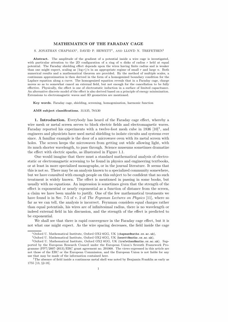
1. Introduction. Everybody has heard of the Faraday cage effect, whereby awire mesh or metal screen serves to block electric fields and electromagnetic waves.Faraday reported his experiments with a twelve-foot mesh cube in 1836 [10]1, andengineers and physicists have used metal shielding to isolate circuits and systems eversince. A familiar example is the door of a microwave oven with its metal screen withholes. The screen keeps the microwaves from getting out while allowing light, withits much shorter wavelength, to pass through. Science museums sometimes dramatizethe effect with electric sparks, as illustrated in Figure 1.1.
One would imagine that there must a standard mathematical analysis of electro-static or electromagnetic screening to be found in physics and engineering textbooks,or at least in more specialized monographs, or in the journal literature. It seems thatthis is not so. There may be an analysis known to a specialized community somewhere,but we have consulted with enough people on this subject to be confident that no suchtreatment is widely known. The effect is mentioned in passing in some books, butusually with no equations. An impression is sometimes given that the strength of theeffect is exponential or nearly exponential as a function of distance from the screen,a claim we have been unable to justify. One of the few mathematical treatments wehave found is in Sec. 7-5 of v. 2 of The Feynman Lectures on Physics [11], where sofar as we can tell, the analysis is incorrect. Feynman considers equal charges ratherthan equal potentials, his wires are of infinitesimal radius, there is no wavelength orindeed external field in his discussion, and the strength of the effect is predicted tobe exponential.
We shall see that there is rapid convergence in the Faraday cage effect, but it isnot what one might expect. As the wire spacing decreases, the field inside the cage
∗Oxford U. Mathematical Institute, Oxford OX2 6GG, UK ([email protected]),†Oxford U. Mathematical Institute, Oxford OX2 6GG, UK ([email protected]),‡Oxford U. Mathematical Institute, Oxford OX2 6GG, UK ([email protected]). Sup-
ported by the European Research Council under the European Union’s Seventh Framework Pro-gramme (FP7/2007–2013)/ERC grant agreement no. 291068. The views expressed in this article arenot those of the ERC or the European Commission, and the European Union is not liable for anyuse that may be made of the information contained here.
1The absence of field inside a continuous metal shell was noted by Benjamin Franklin as early as1755 [13, §2-18].
1
2 S. J. CHAPMAN, D. HEWETT, AND L. N. TREFETHEN
Fig. 1.1. Dramatization of the Faraday cage effect. This image shows the giant Van de Graaffgenerator at the Museum of Science in Boston. (Photo c© Steve Marsel, courtesy of the Museumof Science, Boston.)
converges rapidly not to zero, but to the solution of a homogenized problem involvinga continuum boundary condition. Physically, the boundary condition expresses theproperty that the boundary has limited capacitance since it takes work to push chargeonto small wires.
This paper analyzes the Faraday cage phenomenon from several points of view,and we do not want the reader to lose sight of the main results. Accordingly, theresults are presented in relatively short sections 3–6, with some of the mathematicaldetails deferred to Appendices A–C. The discrete model of Section 6 is simple enoughto be used in teaching, and indeed, it was assigned to 70 Oxford graduate students inthe course “Scientific Computing for DPhil Students” in November 2014.
We note that another paper about Faraday shielding has been published by PaulMartin after discussion with us about some of our results [16].
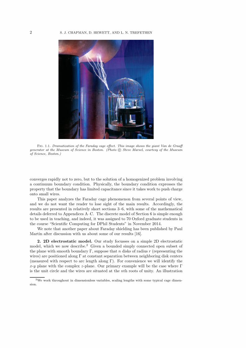
2. 2D electrostatic model. Our study focusses on a simple 2D electrostaticmodel, which we now describe.2 Given a bounded simply connected open subset ofthe plane with smooth boundary Γ, suppose that n disks of radius r (representing thewires) are positioned along Γ at constant separation between neighboring disk centers(measured with respect to arc length along Γ). For convenience we will identify thex-y plane with the complex z-plane. Our primary example will be the case where Γis the unit circle and the wires are situated at the nth roots of unity. An illustration
2We work throughout in dimensionless variables, scaling lengths with some typical cage dimen-sion.
MATHEMATICS OF THE FARADAY CAGE 3
externalfield
smallgradient
n disks of radius rat equal potential
Γ
Fig. 2.1. Model of the Faraday cage in 2D. The curve Γ on which the wires are located, inthis case a circle, is shown as a dashed line.
of the geometry in this case is given in Figure 2.1.We seek a real function φ(z) that satisfies the Laplace equation
∇2φ = 0(2.1)
in the region of the plane exterior to the disks, and the boundary condition
φ = φ0 on the disks.(2.2)
Equation (2.2) asserts that the disks are conducting surfaces at equal potential; here φ0
is an unknown constant to be determined as part of the solution. We emphasize that(2.2) fixes φ(z) to a constant value on disks of finite radius r > 0. This is in contrastto some discussions of screening effects (e.g. [11, §7-5], [24, §7.5.1]) where the wiresare supposed to have infinitesimal radius and are modelled as equal point charges.It is well known in harmonic function theory that Dirichlet boundary conditions canbe imposed on finite-sized boundary components (the precise condition is that eachboundary component must be a set of positive capacity [2]), but not at isolated points.Mathematically, the attempt to specify a potential at an isolated point will generallylead to a problem with no solution. Physically, one may imagine a potential fixed atan isolated point, but its effect will be confined to an infinitesimal region.
We also need to specify some external forcing and appropriate boundary condi-tions at infinity. Our numerical examples will focus on the case where the externalforcing is due to a point charge of strength 2π located at the fixed point z = zs outsideΓ, stipulating that
φ(z) = log(|z − zs|) +O(1) as z → zs,(2.3)
φ(z) = log(|z|) + o(1) as z → ∞.(2.4)
Equation (2.4) implies that the total charge on all the disks is zero, though the chargeon each individual disk will in general be nonzero. Since the charge on a disk is equalto the integral of the normal derviative ∂φ/∂n around its boundary, (2.4) thus impliesthat the sum of these n integrals is zero. (Here n denotes the unit outward normalvector on a curve of integration.)
Our aim is to investigate quantitatively the behavior of the solution φ inside thecage, specifically the magnitude of the associated electric field, ∇φ, as a function of
4 S. J. CHAPMAN, D. HEWETT, AND L. N. TREFETHEN
r = 0.1 r = 0.01 r = 0.001
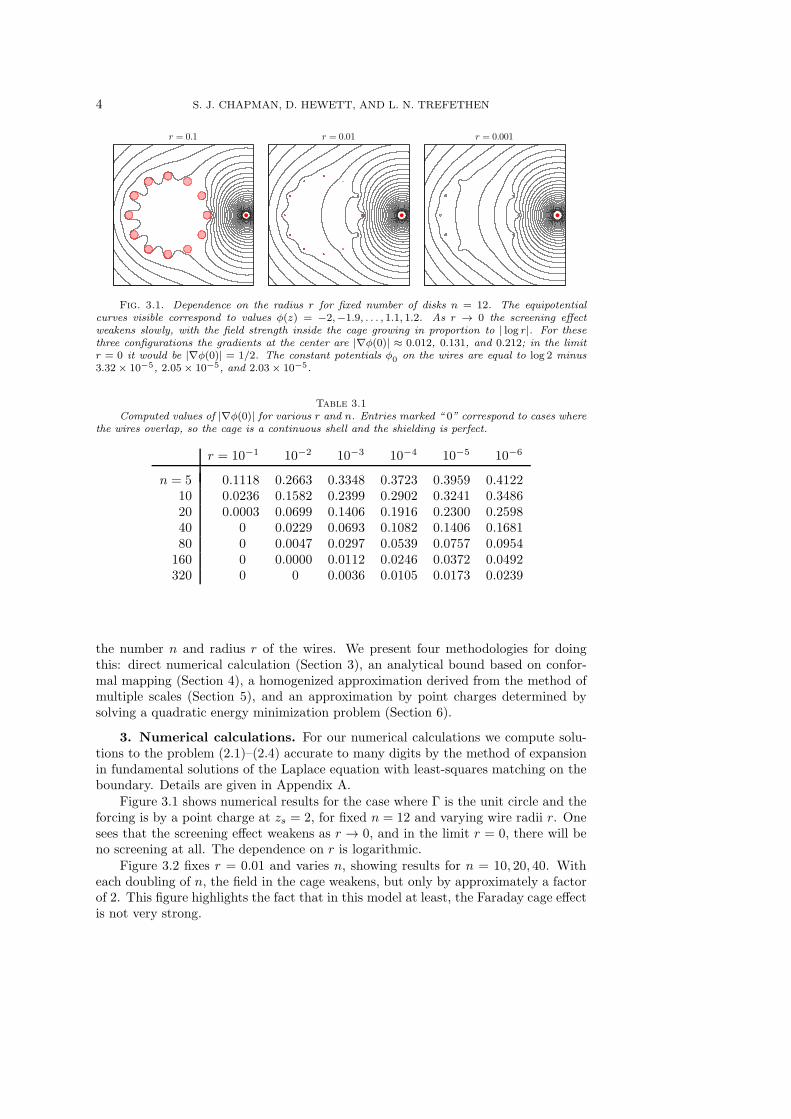
Fig. 3.1. Dependence on the radius r for fixed number of disks n = 12. The equipotentialcurves visible correspond to values φ(z) = −2,−1.9, . . . , 1.1, 1.2. As r → 0 the screening effectweakens slowly, with the field strength inside the cage growing in proportion to | log r|. For thesethree configurations the gradients at the center are |∇φ(0)| ≈ 0.012, 0.131, and 0.212; in the limitr = 0 it would be |∇φ(0)| = 1/2. The constant potentials φ
0on the wires are equal to log 2 minus
3.32× 10⁻⁵, 2.05× 10⁻⁵, and 2.03× 10⁻⁵.
Table 3.1
Computed values of |∇φ(0)| for various r and n. Entries marked “ 0” correspond to cases wherethe wires overlap, so the cage is a continuous shell and the shielding is perfect.
r = 10−1 10−2 10−3 10−4 10−5 10−6
n = 5 0.1118 0.2663 0.3348 0.3723 0.3959 0.412210 0.0236 0.1582 0.2399 0.2902 0.3241 0.348620 0.0003 0.0699 0.1406 0.1916 0.2300 0.259840 0 0.0229 0.0693 0.1082 0.1406 0.168180 0 0.0047 0.0297 0.0539 0.0757 0.0954
160 0 0.0000 0.0112 0.0246 0.0372 0.0492320 0 0 0.0036 0.0105 0.0173 0.0239
the number n and radius r of the wires. We present four methodologies for doingthis: direct numerical calculation (Section 3), an analytical bound based on confor-mal mapping (Section 4), a homogenized approximation derived from the method ofmultiple scales (Section 5), and an approximation by point charges determined bysolving a quadratic energy minimization problem (Section 6).
3. Numerical calculations. For our numerical calculations we compute solu-tions to the problem (2.1)–(2.4) accurate to many digits by the method of expansionin fundamental solutions of the Laplace equation with least-squares matching on theboundary. Details are given in Appendix A.
Figure 3.1 shows numerical results for the case where Γ is the unit circle and theforcing is by a point charge at zs = 2, for fixed n = 12 and varying wire radii r. Onesees that the screening effect weakens as r → 0, and in the limit r = 0, there will beno screening at all. The dependence on r is logarithmic.
Figure 3.2 fixes r = 0.01 and varies n, showing results for n = 10, 20, 40. Witheach doubling of n, the field in the cage weakens, but only by approximately a factorof 2. This figure highlights the fact that in this model at least, the Faraday cage effectis not very strong.
MATHEMATICS OF THE FARADAY CAGE 5
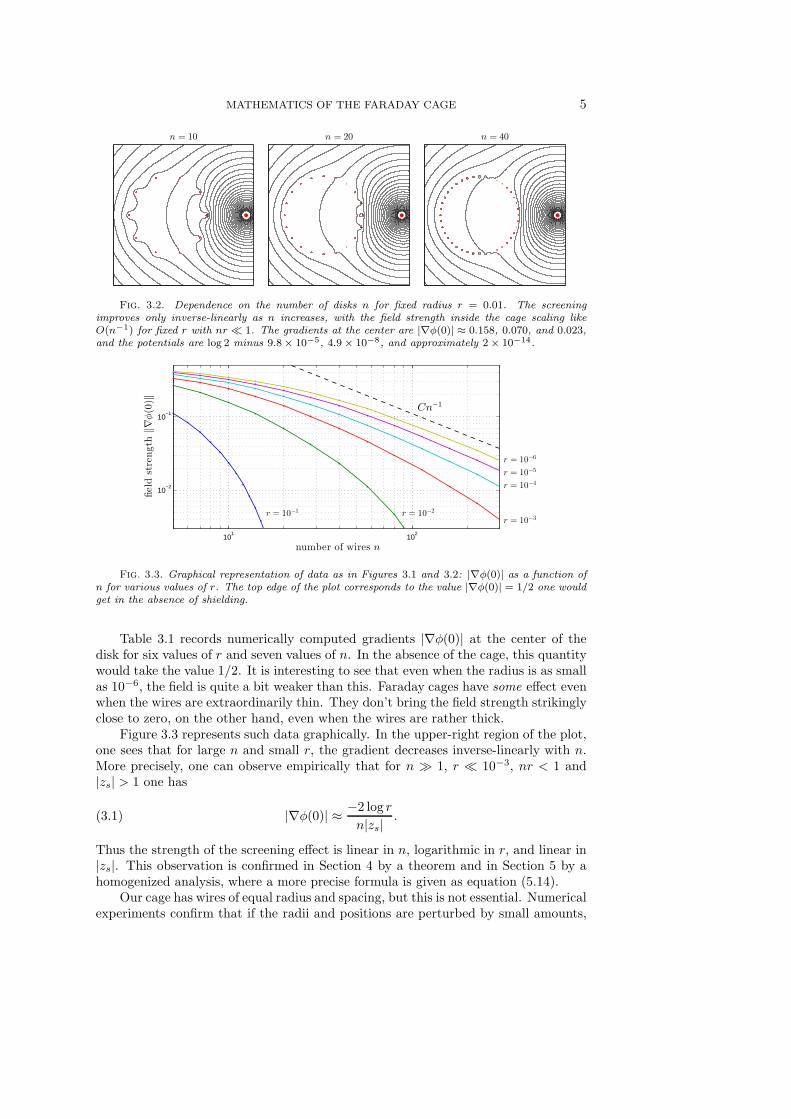
n = 10 n = 20 n = 40
Fig. 3.2. Dependence on the number of disks n for fixed radius r = 0.01. The screeningimproves only inverse-linearly as n increases, with the field strength inside the cage scaling likeO(n−1) for fixed r with nr ≪ 1. The gradients at the center are |∇φ(0)| ≈ 0.158, 0.070, and 0.023,and the potentials are log 2 minus 9.8× 10⁻⁵, 4.9× 10⁻⁸, and approximately 2× 10⁻¹⁴.
101
102
10−2
10−1
fieldstrength
‖∇φ(0)‖
number of wires n
Cn−1
r = 10−1 r = 10−2r = 10−3
r = 10−4r = 10−5r = 10−6
Fig. 3.3. Graphical representation of data as in Figures 3.1 and 3.2: |∇φ(0)| as a function ofn for various values of r. The top edge of the plot corresponds to the value |∇φ(0)| = 1/2 one wouldget in the absence of shielding.
Table 3.1 records numerically computed gradients |∇φ(0)| at the center of thedisk for six values of r and seven values of n. In the absence of the cage, this quantitywould take the value 1/2. It is interesting to see that even when the radius is as smallas 10−6, the field is quite a bit weaker than this. Faraday cages have some effect evenwhen the wires are extraordinarily thin. They don’t bring the field strength strikinglyclose to zero, on the other hand, even when the wires are rather thick.
Figure 3.3 represents such data graphically. In the upper-right region of the plot,one sees that for large n and small r, the gradient decreases inverse-linearly with n.More precisely, one can observe empirically that for n ≫ 1, r ≪ 10−3, nr < 1 and|zs| > 1 one has
|∇φ(0)| ≈−2 log r
n|zs|.(3.1)
Thus the strength of the screening effect is linear in n, logarithmic in r, and linear in|zs|. This observation is confirmed in Section 4 by a theorem and in Section 5 by ahomogenized analysis, where a more precise formula is given as equation (5.14).
Our cage has wires of equal radius and spacing, but this is not essential. Numericalexperiments confirm that if the radii and positions are perturbed by small amounts,
6 S. J. CHAPMAN, D. HEWETT, AND L. N. TREFETHEN
the fields do not change very much.
4. Theorem. By combining known bounds for harmonic functions with certainconformal transplantations, it is possible to derive a theorem that confirms the numer-ical observation (3.1). Rather than restrict attention to the specific forcing functionlog(|z−zs|), we now imagine a Faraday cage on the unit circle subject to an arbitraryforcing field outside the disk of radius R > 1. Specifically, given R > 1, let φ be aharmonic function satisfying |φ(z)| < 1 in the region |z| < R minus the n disks ofradius r, where it takes the constant value φ(z) = 0. Appendix B establishes thefollowing bound.
Theorem 1. Given R > 1, n ≥ 4, and r ≤ 1/n, let φ be a harmonic function
satisfying |φ(z)| ≤ 1 in the region Ω consisting of the disk |z| < R punctured by the ndisks of radius r centered at the nth roots of unity, where φ takes a constant value φ0
between −1 and 1. Then
|∇φ(0)| ≤4 | log r |
n logR.(4.1)
Although this theorem as stated gives a bound on the gradient just for z = 0,the argument can be extended to a similar bound for any z with |z| < 1 − r, withconstants weakening by a factor proportional to (1 − r − |z|)−1. We note also thatalthough the theorem gives a bound of order 1/ logR for large R, the actual scalingis smaller than this, of order 1/R, as in (3.1).
5. Continuum approximation. In Figures 3.1–3.2 it is evident that inside theFaraday cage, though the potential is not very close to a constant, it is close to some
smooth function, except just next to the wires. Under appropriate assumptions, onecan make this observation precise, approximating the cage by a continuum modelwith an effective boundary condition on the curve Γ. Details of our derivation bythe method of multiple scales are given in Appendix C. Related effective boundaryconditions have been obtained for problems with discontinuities along layers by themethod of “generalized impedance boundary conditions” as discussed for examplein [3, 9, 21]. The closest treatment we know of to our own is that of Delourme etal. [6, 7, 8].
The homogenized approximation can be described as follows. Suppose the con-stant separation between neighboring wire centers (measured with respect to arclength along Γ) is ε = |Γ|/n ≪ 1, where |Γ| is the total arc length, and the radius ofeach wire is r ≪ ε. The crucial scaling parameter that determines the effectiveness ofthe screening is
α =2π
ε log(ε/2πr).(5.1)
If ε ≫ 1/ log(ε/r), then α ≪ 1 and the wires are too thin for effective screening. Ifε ≪ 1/ log(ε/r), then α ≫ 1 and the screening is strong. Specifically, here is thecontinuum problem that results from our asymptotic analysis. Away from Γ, theleading order solution satisfies the Laplace equation. On Γ, φ is continuous, but itsnormal derivative satisfies a jump condition:
[
∂φ
∂n
]
= α(φ− φ0) on Γ,(5.2)
MATHEMATICS OF THE FARADAY CAGE 7
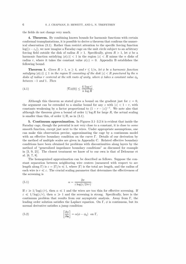
Fig. 5.1. Analogue of Figure 3.1 for the continuum approximation determined by (5.1) and(5.5)–(5.9). Again the number of disks is fixed at n = 12 and the radius r varies. Note the strikingagreement of the two images shown with those of Figure 3.1, corresponding to values α = 5.660 and2.713. The first image is absent because in this case rn > 1, making α negative and the homogenizedapproximation inapplicable. The mean potential φ
0of (5.7) is log 2 ≈ 0.693.
where φ0, to be determined, is the mean value of φ on Γ. Here [f ] denotes the jumpin f across Γ, from exterior to interior, and n is the unit outward normal vector on Γ.Note that for α ≪ 1, (5.2) implies that ∂φ/∂n barely jumps across Γ: the screeningis weak. For α ≫ 1, (5.2) implies that φ is almost constant along Γ: the screening isstrong.
Equation (5.2) can be given a physical interpretation, if we recall that across acurve supporting a charge distribution of density ρ, the gradient of a potential jumpsby ρ. Thus another way to write (5.2) is
ρ = α(φ− φ0) on Γ,(5.3)
where ρ, a function of z, is the charge density along Γ. The parameter α, a ratio ofcharge to voltage, can be interpreted as a capacitance per unit length. For a perfectshell with α = ∞, ρ is such that φ = φ0 along Γ, so the external field is exactlycancelled, but for finite α, ρ does not adjust so far.
Solving for r in (5.1) gives
r =ε
2πe−2π/αε.(5.4)
In other words, the distinguished limit in which α is strictly of order one occurs whenr ∼ εA exp(−c/ε) as ε → 0 for some constants A, c > 0 (in which case α ∼ 2π/c).Essentially the same critical scaling is derived in [19, 20] for problems of electrostaticscreening and by rigorous homogenization theory in [5] in the context of a much moregeneral discussion of limiting behavior of solutions of partial differential equations indomains with microstructure.
For the cage subject to a point charge as in Section 2, the homogenized modeltakes the following form:
∇2φ = 0 in R2 \ Γ ∪ zs,(5.5)
[φ] = 0 on Γ,(5.6)
[
∂φ
∂n
]
= α(φ − φ0) on Γ,(5.7)
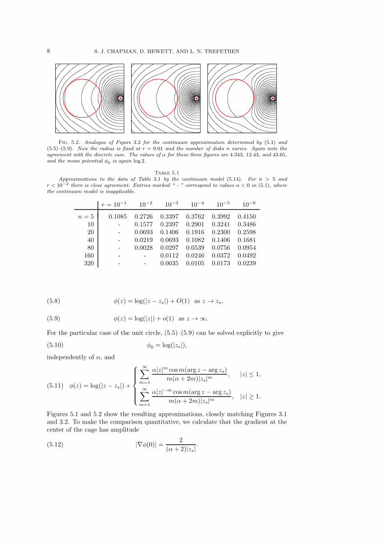
8 S. J. CHAPMAN, D. HEWETT, AND L. N. TREFETHEN
Fig. 5.2. Analogue of Figure 3.2 for the continuum approximation determined by (5.1) and(5.5)–(5.9). Now the radius is fixed at r = 0.01 and the number of disks n varies. Again note theagreement with the discrete case. The values of α for these three figures are 4.343, 12.43, and 43.65,and the mean potential φ
0is again log 2.
Table 5.1
Approximations to the data of Table 3.1 by the continuum model (5.14). For n > 5 andr < 10−2 there is close agreement. Entries marked “ - ” correspond to values α < 0 in (5.1), wherethe continuum model is inapplicable.
r = 10−1 10−2 10−3 10−4 10−5 10−6
n = 5 0.1085 0.2726 0.3397 0.3762 0.3992 0.415010 - 0.1577 0.2397 0.2901 0.3241 0.348620 - 0.0693 0.1406 0.1916 0.2300 0.259840 - 0.0219 0.0693 0.1082 0.1406 0.168180 - 0.0028 0.0297 0.0539 0.0756 0.0954
160 - - 0.0112 0.0246 0.0372 0.0492320 - - 0.0035 0.0105 0.0173 0.0239
φ(z) = log(|z − zs|) +O(1) as z → zs,(5.8)
φ(z) = log(|z|) + o(1) as z → ∞.(5.9)
For the particular case of the unit circle, (5.5)–(5.9) can be solved explicitly to give
φ0 = log(|zs|),(5.10)
independently of α, and
φ(z) = log(|z − zs|) +
∞∑
m=1
α|z|m cosm(arg z − arg zs)
m(α+ 2m)|zs|m, |z| ≤ 1,
∞∑
m=1
α|z|−m cosm(arg z − arg zs)
m(α+ 2m)|zs|m, |z| ≥ 1.
(5.11)
Figures 5.1 and 5.2 show the resulting approximations, closely matching Figures 3.1and 3.2. To make the comparison quantitative, we calculate that the gradient at thecenter of the cage has amplitude
|∇φ(0)| =2
(α+ 2)|zs|.(5.12)
MATHEMATICS OF THE FARADAY CAGE 9
101
102
10−2
10−1
fieldstrength
‖∇φ(0)‖
number of wires n
Cn−1
r = 10−1
r = 10−2r = 10−3
r = 10−4r = 10−5r = 10−6
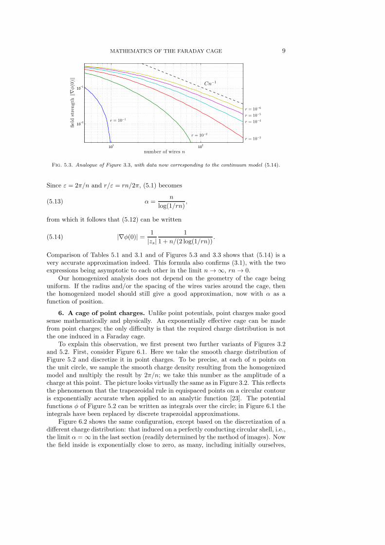
Fig. 5.3. Analogue of Figure 3.3, with data now corresponding to the continuum model (5.14).
Since ε = 2π/n and r/ε = rn/2π, (5.1) becomes
α =n
log(1/rn),(5.13)
from which it follows that (5.12) can be written
|∇φ(0)| =1
|zs|
1
1 + n/(2 log(1/rn)).(5.14)
Comparison of Tables 5.1 and 3.1 and of Figures 5.3 and 3.3 shows that (5.14) is avery accurate approximation indeed. This formula also confirms (3.1), with the twoexpressions being asymptotic to each other in the limit n → ∞, rn → 0.
Our homogenized analysis does not depend on the geometry of the cage beinguniform. If the radius and/or the spacing of the wires varies around the cage, thenthe homogenized model should still give a good approximation, now with α as afunction of position.
6. A cage of point charges. Unlike point potentials, point charges make goodsense mathematically and physically. An exponentially effective cage can be madefrom point charges; the only difficulty is that the required charge distribution is notthe one induced in a Faraday cage.
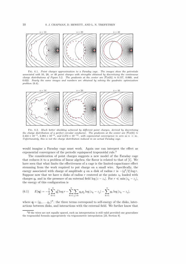
To explain this observation, we first present two further variants of Figures 3.2and 5.2. First, consider Figure 6.1. Here we take the smooth charge distribution ofFigure 5.2 and discretize it in point charges. To be precise, at each of n points onthe unit circle, we sample the smooth charge density resulting from the homogenizedmodel and multiply the result by 2π/n; we take this number as the amplitude of acharge at this point. The picture looks virtually the same as in Figure 3.2. This reflectsthe phenomenon that the trapezeoidal rule in equispaced points on a circular contouris exponentially accurate when applied to an analytic function [23]. The potentialfunctions φ of Figure 5.2 can be written as integrals over the circle; in Figure 6.1 theintegrals have been replaced by discrete trapezoidal approximations.
Figure 6.2 shows the same configuration, except based on the discretization of adifferent charge distribution: that induced on a perfectly conducting circular shell, i.e.,the limit α = ∞ in the last section (readily determined by the method of images). Nowthe field inside is exponentially close to zero, as many, including initially ourselves,
10 S. J. CHAPMAN, D. HEWETT, AND L. N. TREFETHEN
n = 10 n = 20 n = 40
Fig. 6.1. Point charges approximation to a Faraday cage. The images show the potentialsassociated with 10, 20, or 40 point charges with strengths obtained by discretizing the continuouscharge distributions of Figure 5.2. The gradients at the center are |∇φ(0)| ≈ 0.157, 0.069, and0.022. Nearly the same images and numbers are obtained by solving the quadratic optimizationproblem (6.4).
n = 10 n = 20 n = 40
Fig. 6.2. Much better shielding achieved by different point charges, derived by discretizingthe charge distribution of a perfect circular conductor. The gradients at the center are |∇φ(0)| ≈2.444 × 10⁻³, 2.384 × 10⁻⁶, and 2.274 × 10⁻¹², with exponential convergence to zero as n → ∞.Unfortunately, this is not the charge distribution induced in an actual Faraday cage.
would imagine a Faraday cage must work. Again one can interpret the effect asexponential convergence of the periodic equispaced trapezoidal rule.3
The consideration of point charges suggests a new model of the Faraday cagethat reduces it to a problem of linear algebra; the flavor is related to that of [1]. Wehave seen that what limits the effectiveness of a cage is the limited-capacitance effectstemming from the work required to put charge on a small wire. Specifically, theenergy associated with charge of amplitude q on a disk of radius r is −(q2/2) log r.Suppose now that we have n disks of radius r centered at the points zk loaded withcharges qk and in the presence of an external field log |z − zs|. For r ≪ min |zk − zj |,the energy of this configuration is
E(q) = −1
2
n∑
k=1
q2k log r −
n∑
k=1
∑
j>k
qkqj log |zk − zj| −
n∑
k=1
qk log |zk − zs|,(6.1)
where q = (q1, . . . qn)T : the three terms correspond to self-energy of the disks, inter-
actions between disks, and interactions with the external field. We further know that
3If the wires are not equally spaced, such an interpretation is still valid provided one generalizesthe trapezoidal formula appropriately via trigonometric interpolation [23, Section 9].
MATHEMATICS OF THE FARADAY CAGE 11
the total charge on all the wires is zero,
n∑
k=1
qk = 0.(6.2)
This formulation suggests that we can find the charges qk by minimizing the quadraticform E(q) over all n-vectors q satisfying (6.2). This is a constrained quadratic pro-gramming problem of the form
E(q) =1
2qTAq− fTq , cTq = 0,(6.3)
for a suitable matrix A and vectors f and c, with solution vector q satisfying the block2× 2 linear system
(
A c
cT 0
)(
q
λ
)
=
(
f
0
)
;(6.4)
here λ is a Lagrange multiplier. Solving (6.4) for q leads to a cage of point chargeswhose potentials look essentially the same as in Figures 3.2 and 6.1 (not shown).
7. Discussion. This article has investigated an electrostatic problem. Our anal-ysis shows that the shielding improves only linearly as the spacing between wires of acage shrinks, and this is probably why your cell phone often works inside an elevator.The shielding also depends on having wires of finite thickness, and this is probablywhy it is hard to see into your microwave oven. (If thin wires provided good enoughshielding, the designers of microwave oven doors would use them.) Bjorn Engquisthas pointed out to us an amusing illustration of the challenges of Faraday shieldingthat combines both of these devices. Put your cell phone inside your microwave oven,close the door, and give it a call. The phone will ring merrily!
In particular, we have found that the Faraday shielding effect can be accuratelymodeled by a homogenized problem with a continuous boundary condition, whichexpresses the fact that the boundary has limited capacitance since it takes work toforce charge onto narrow wires. This capacitance observation in turn suggests evensimpler models based on energy minimization. We presented such a model in a discretecontext in Section 6, and a continuous argument of limited capacitance and energyminimization could also be developed.
The overall structure of our arguments is summarized in Figure 7.1. Let usquickly mention yet another argument, suggested by Toby Driscoll, that explains instill another way that Faraday shielding must be weak. Consider the configurationof a circular shell that is complete except for a single gap of size ε. By a conformalmap, one can calculate the potential inside this shell exactly, and the gradient in theinterior comes out of magnitude O(ε2). Clearly the cage of n gaps will have weakerscreening than this screen of one gap: weaker, as we have seen, by a factor O(ε−1)corresponding to the number of gaps.
It has surprised us deeply in the course of this work to find no mathematicalanalysis of the Faraday cage effect in the literature, despite its age, fame, and practicalimportance. Feynman’s treatment alone must have been read by tens of thousands ofstudents and physicists, which may have contributed to the widespread misconceptionthat the shielding is exponential. Curiously, Maxwell in his 1873 treatise consideredthe same special case of an infinite planar array of wires and got it right, including the
12 S. J. CHAPMAN, D. HEWETT, AND L. N. TREFETHEN
True problem
Point charges approximation
Homogenized approximation
POINT SAMPLING
À LA TRAPEZOIDAL RULE
screening is weak and depends on r
far from a perfect conductor far from optimal screening
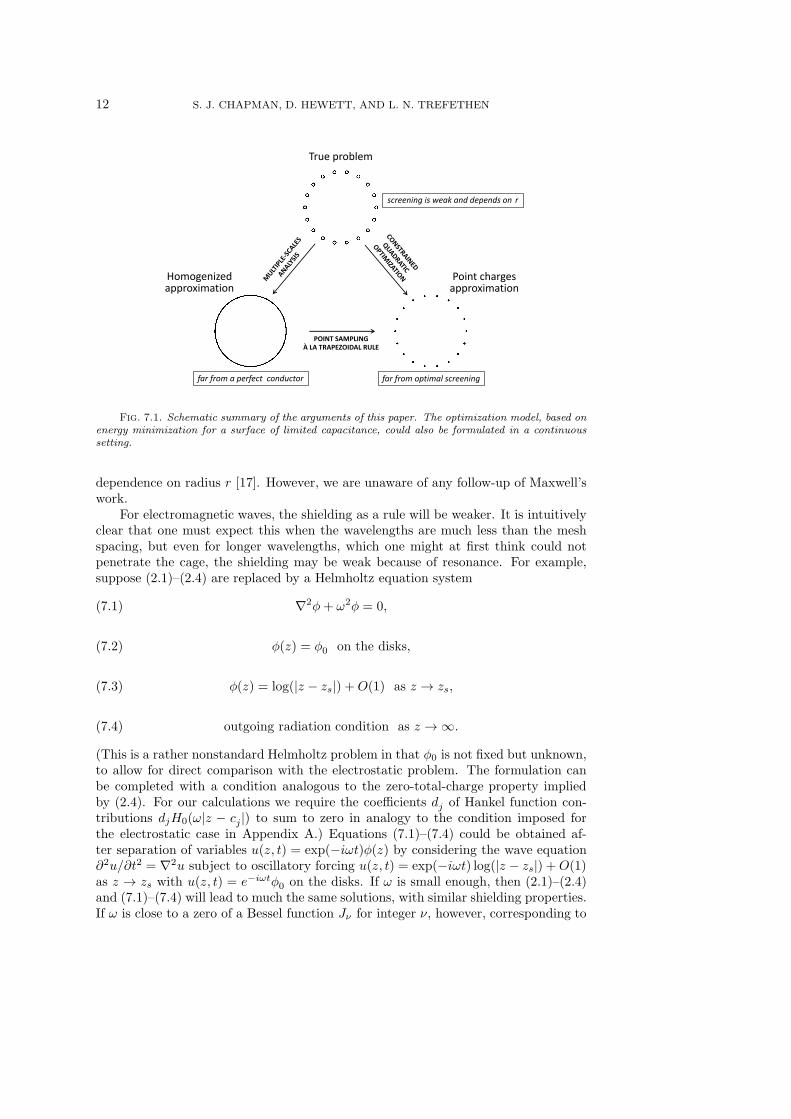
Fig. 7.1. Schematic summary of the arguments of this paper. The optimization model, based onenergy minimization for a surface of limited capacitance, could also be formulated in a continuoussetting.
dependence on radius r [17]. However, we are unaware of any follow-up of Maxwell’swork.
For electromagnetic waves, the shielding as a rule will be weaker. It is intuitivelyclear that one must expect this when the wavelengths are much less than the meshspacing, but even for longer wavelengths, which one might at first think could notpenetrate the cage, the shielding may be weak because of resonance. For example,suppose (2.1)–(2.4) are replaced by a Helmholtz equation system
∇2φ+ ω2φ = 0,(7.1)
φ(z) = φ0 on the disks,(7.2)
φ(z) = log(|z − zs|) +O(1) as z → zs,(7.3)
outgoing radiation condition as z → ∞.(7.4)
(This is a rather nonstandard Helmholtz problem in that φ0 is not fixed but unknown,to allow for direct comparison with the electrostatic problem. The formulation canbe completed with a condition analogous to the zero-total-charge property impliedby (2.4). For our calculations we require the coefficients dj of Hankel function con-tributions djH0(ω|z − cj|) to sum to zero in analogy to the condition imposed forthe electrostatic case in Appendix A.) Equations (7.1)–(7.4) could be obtained af-ter separation of variables u(z, t) = exp(−iωt)φ(z) by considering the wave equation∂2u/∂t2 = ∇2u subject to oscillatory forcing u(z, t) = exp(−iωt) log(|z − zs|) +O(1)as z → zs with u(z, t) = e−iωtφ0 on the disks. If ω is small enough, then (2.1)–(2.4)and (7.1)–(7.4) will lead to much the same solutions, with similar shielding properties.If ω is close to a zero of a Bessel function Jν for integer ν, however, corresponding to
MATHEMATICS OF THE FARADAY CAGE 13
ω = 0.5 ω = 2.2 ω = 2.8
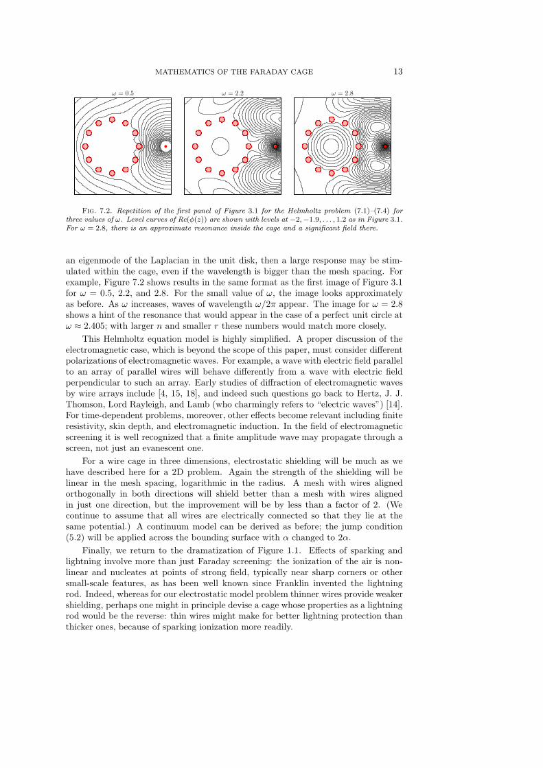
Fig. 7.2. Repetition of the first panel of Figure 3.1 for the Helmholtz problem (7.1)–(7.4) forthree values of ω. Level curves of Re(φ(z)) are shown with levels at −2,−1.9, . . . , 1.2 as in Figure 3.1.For ω = 2.8, there is an approximate resonance inside the cage and a significant field there.
an eigenmode of the Laplacian in the unit disk, then a large response may be stim-ulated within the cage, even if the wavelength is bigger than the mesh spacing. Forexample, Figure 7.2 shows results in the same format as the first image of Figure 3.1for ω = 0.5, 2.2, and 2.8. For the small value of ω, the image looks approximatelyas before. As ω increases, waves of wavelength ω/2π appear. The image for ω = 2.8shows a hint of the resonance that would appear in the case of a perfect unit circle atω ≈ 2.405; with larger n and smaller r these numbers would match more closely.
This Helmholtz equation model is highly simplified. A proper discussion of theelectromagnetic case, which is beyond the scope of this paper, must consider differentpolarizations of electromagnetic waves. For example, a wave with electric field parallelto an array of parallel wires will behave differently from a wave with electric fieldperpendicular to such an array. Early studies of diffraction of electromagnetic wavesby wire arrays include [4, 15, 18], and indeed such questions go back to Hertz, J. J.Thomson, Lord Rayleigh, and Lamb (who charmingly refers to “electric waves”) [14].For time-dependent problems, moreover, other effects become relevant including finiteresistivity, skin depth, and electromagnetic induction. In the field of electromagneticscreening it is well recognized that a finite amplitude wave may propagate through ascreen, not just an evanescent one.
For a wire cage in three dimensions, electrostatic shielding will be much as wehave described here for a 2D problem. Again the strength of the shielding will belinear in the mesh spacing, logarithmic in the radius. A mesh with wires alignedorthogonally in both directions will shield better than a mesh with wires alignedin just one direction, but the improvement will be by less than a factor of 2. (Wecontinue to assume that all wires are electrically connected so that they lie at thesame potential.) A continuum model can be derived as before; the jump condition(5.2) will be applied across the bounding surface with α changed to 2α.
Finally, we return to the dramatization of Figure 1.1. Effects of sparking andlightning involve more than just Faraday screening: the ionization of the air is non-linear and nucleates at points of strong field, typically near sharp corners or othersmall-scale features, as has been well known since Franklin invented the lightningrod. Indeed, whereas for our electrostatic model problem thinner wires provide weakershielding, perhaps one might in principle devise a cage whose properties as a lightningrod would be the reverse: thin wires might make for better lightning protection thanthicker ones, because of sparking ionization more readily.
14 S. J. CHAPMAN, D. HEWETT, AND L. N. TREFETHEN
% Solve the problem:
n = 12; r = 0.1; % number and radius of disks
c = exp(2i*pi*(1:n)/n); % centers of the disks
rr = r*ones(size(c)); % vector of radii
N = max(0,round(4+.5*log10(r))); % number of terms in expansions
npts = 3*N+2; % number of sample points on circles
circ = exp((1:npts)’*2i*pi/npts); % roots of unity for collocation
z = []; for j = 1:n
z = [z; c(j)+rr(j)*circ]; end % collocation points
A = [0; -ones(size(z))]; % the constant term
zs = 2; % location of the singularity
rhs = [0; -log(abs(z-zs))]; % right-hand side
for j = 1:n
A = [A [1; log(abs(z-c(j)))]]; % the logarithmic terms
for k = 1:N
zck = (z-c(j)).^(-k);
A = [A [0;real(zck)] [0;imag(zck)]]; % the algebraic terms
end
end
X = A\rhs; % solve least-squares problem
e = X(1); X(1) =[]; % constant potential on wires
d = X(1:2*N+1:end); X(1:2*N+1:end) = []; % coeffs of log terms
a = X(1:2:end); b = X(2:2:end); % coeffs of algebraic terms
% Plot the solution:
x = linspace(-1.4,2.2,120); y = linspace(-1.8,1.8,120);
[xx,yy] = meshgrid(x,y); zz = xx+1i*yy; uu = log(abs(zz-zs));
for j = 1:n
uu = uu+d(j)*log(abs(zz-c(j)));
for k = 1:N, zck = (zz-c(j)).^(-k); kk = k+(j-1)*N;
uu = uu+a(kk)*real(zck)+b(kk)*imag(zck); end
end
for j = 1:n, uu(abs(zz-c(j))<rr(j)) = NaN; end
z = exp(pi*1i*(-50:50)’/50);
for j = 1:n, disk = c(j)+rr(j)*z; fill(real(disk),imag(disk),[1 .7 .7])
hold on, plot(disk,’-r’), end
contour(xx,yy,uu,-2:.1:1.2), colormap([0 0 0]), axis([-1.4 2.2 -1.8 1.8])
axis square, plot(real(zs),imag(zs),’.r’)
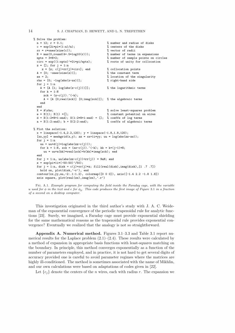
Fig. A.1. Example program for computing the field inside the Faraday cage, with the variableu used for φ in the text and e for φ
0. This code produces the first image of Figure 3.1 in a fraction
of a second on a desktop computer.
This investigation originated in the third author’s study with J. A. C. Weide-man of the exponential convergence of the periodic trapezoidal rule for analytic func-tions [23]. Surely, we imagined, a Faraday cage must provide exponential shieldingfor the same mathematical reasons as the trapezoidal rule provides exponential con-vergence? Eventually we realized that the analogy is not so straightforward.
Appendix A. Numerical method. Figures 3.1–3.3 and Table 3.1 report nu-merical results for the Laplace problem (2.1)–(2.4). These results were calculated bya method of expansion in appropriate basis functions with least-squares matching onthe boundary. In principle, this method converges exponentially as a function of thenumber of parameters employed, and in practice, it is not hard to get several digits ofaccuracy provided one is careful to avoid parameter regimes where the matrices arehighly ill-conditioned. The method is sometimes associated with the name of Mikhlin,and our own calculations were based on adaptations of codes given in [22].
Let cj denote the centers of the n wires, each with radius r. The expansion we
MATHEMATICS OF THE FARADAY CAGE 15
utilize takes the form
φ(z) = log |z − zs|+
n∑
j=1
dj log |z − cj |+Re
[
N∑
k=1
(ajk − ibjk)(z − cj)−k
]
,(A.1)
where dj, ajk, and bjk are real constants to be determined along with e = φ0,the constant voltage on the wires in (2.2)). We fix d1 by the condition
∑
dj = 0, whichis equivalent to (2.4), and the rest of the parameters are unknowns. The number Nis taken large enough for good accuracy but not so large as to make the matricestoo ill-conditioned (especially an issue when r is small): our experimentally derivedrule of thumb is to take N as the nonnegative integer closest to 4 + 0.5 log10(r).For any coefficients, the function (A.1) satisfies (2.1), (2.3) and (2.4), and our aimis to find coefficients so that it also satisfies (2.2). To this end, the boundary ofeach disk is discretized in a number of points, typically 3N + 2, which makes (2.2)into an overdetermined linear system of equations involving a matrix of dimension(3nN+2n+1)× (2nN+n+1). This problem is then solved by the standard methodsinvoked by the MATLAB backslash command. A sample MATLAB code is listed inFigure A.1.
For the Helmholtz equation of Section 7, the computations are similar but based
on Hankel functions of the first kind H(1)j rather than logarithms and inverse powers.
Appendix B. Proof of Theorem 1. To begin the proof, assume φ0 = 0. Underthis assumption we claim that φ satisfies
|φ(ζ)| ≤| log r |
n logR, |ζ| ≤ 1, ζ ∈ Ω.(B.1)
To prove this, we note that for each ζ ∈ Ω, φ(ζ) is a weighted average of the values ofφ(z) on the boundary ∂Ω; the weighting function is known as the harmonic measure
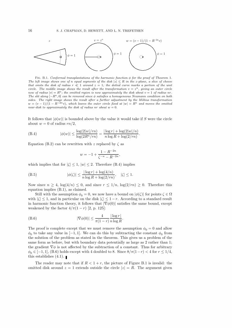
associated with the point ζ. It follows that for any ζ ∈ Ω, the largest value that |φ(ζ)|may take under the given assumptions on the boundary data is equal to the valuetaken by φ(ζ) in the case where φ(z) = 1 identically for |z| = R. (Equivalently, itis the harmonic measure of the boundary circle |z| = R for the given ζ and Ω.) Wecan estimate this number by making use of the transformation v = zn followed byw = (v − 1)/(1−R−2nv), as indicated in Figure B.1:
w =zn − 1
1−R−2nzn.(B.2)
Under this transformation, the solution φ(w) to the Dirichlet problem in the regionon the right of the figure corresponds pointwise to the solution in the left region,φ(z). (We abuse notation slightly by using the same symbol φ in the z, v, and wdomains.) The region on the right is bounded on the outside by the circle |w| = Rn,with φ(w) = 1, and on the inside by a curve S that is approximately the circlew : |w| = rn, with φ(w) = 0. The minimal absolute value of points w ∈ S is thevalue corresponding to z = 1− r,
|w|min =1− (1− r)n
1−R−2n(1− r)n,(B.3)
and an easy estimate using the assumption r < 1/n gives
|w|min ≥rn
2.
16 S. J. CHAPMAN, D. HEWETT, AND L. N. TREFETHEN
z
φ = 1
v = zn
φ = 1
w = (v − 1)/(1 − R−2nv)
φ = 1
Fig. B.1. Conformal transplantations of the harmonic function φ for the proof of Theorem 1.The left image shows one of n equal segments of the disk |z| ≤ R in the z-plane, a slice of cheesethat omits the disk of radius r ≪ 1 around z = 1; the dotted curve marks a portion of the unitcircle. The middle image shows the result after the transformation v = zn, giving an outer circlenow of radius |v| = Rn; the omitted region is now approximately the disk about v = 1 of radius nr.The slit along [−Rn, 0] can be removed since φ satisfies a homogeneous Neumann condition on bothsides. The right image shows the result after a further adjustment by the Mobius transformationw = (v − 1)/(1 − R−2nv), which leaves the outer circle fixed at |w| = Rn and moves the omittednear-disk to approximately the disk of radius nr about w = 0.
It follows that |φ(w)| is bounded above by the value it would take if S were the circleabout w = 0 of radius rn/2,
|φ(w)| ≤log(2|w|/rn)
log(2Rn/rn)=
| log r |+ log(2|w|/n)
n logR+ log(2/rn).(B.4)
Equation (B.2) can be rewritten with z replaced by ζ as
w = −1 +1−R−2n
ζ−n − R−2n,
which implies that for |ζ| ≤ 1, |w| ≤ 2. Therefore (B.4) implies
|φ(ζ)| ≤| log r |+ log(4/n)
n logR+ log(2/rn), |ζ| ≤ 1.(B.5)
Now since n ≥ 4, log(4/n) ≤ 0, and since r ≤ 1/n, log(2/rn) ≥ 0. Therefore thisequation implies (B.1), as claimed.
Still with the assumption φ0 = 0, we now have a bound on |φ(ζ)| for points ζ ∈ Ωwith |ζ| ≤ 1, and in particular on the disk |ζ| ≤ 1− r. According to a standard resultin harmonic function theory, it follows that |∇φ(0)| satisfies the same bound, exceptweakened by the factor 4/π(1− r) [2, p. 125]:
|∇φ(0)| ≤4
π(1− r)
| log r |
n logR.(B.6)
The proof is complete except that we must remove the assumption φ0 = 0 and allowφ0 to take any value in [−1, 1]. We can do this by subtracting the constant φ0 fromthe solution of the problem as stated in the theorem. This gives us a problem of thesame form as before, but with boundary data potentially as large as 2 rather than 1;the gradient ∇φ is not affected by the subtraction of a constant. Thus for arbitraryφ0 ∈ [−1, 1], (B.6) holds except with 4 doubled to 8. Since 8/π(1−r) < 4 for r ≤ 1/4,this establishes (4.1).
The reader may note that if R < 1 + r, the picture of Figure B.1 is invalid: theomitted disk around z = 1 extends outside the circle |z| = R. The argument given
MATHEMATICS OF THE FARADAY CAGE 17
remains valid, nevertheless, with Ω now defined as that portion of the disk |z| < Rthat is disjoint from the n disks of radius r centered at the nth roots of unity.
Appendix C. Derivation of homogenized equation. Our method is multiplescales analysis, as described for example in [12]. We present the analysis for a verticalline of circular disks of radius r = δǫ, δ ≪ 1, centered on the straight line x = 0 at thepoints (0, kǫ) for k ∈ Z. The generalisation to an arbitrary curve is straightforward.Addition of a constant to the potential does not change the problem significantly, sofor simplicity we look for a solution φ that is zero on the disks.
There are three asymptotic regions that make up the solution. First, there is anouter region away from the cage, in which x = O(1). This region will see the cageas an effective boundary condition, leading to the problem (5.5)–(5.9). Second, thereis a boundary layer region, in which x = O(ǫ). In this region the discrete natureof the wires becomes apparent, but they are of vanishing thickness and act as pointcharges. The solution here is of multiple-scales form in y, with fast scale O(ǫ) andslow scale O(1). Third, there is an inner region near a single wire, in which x = O(δǫ),y = O(δǫ). This region determines the induced charge on the wire resulting from theequipotential condition.
The multiple scales form of the solution in y means that it is written in terms ofa slow variable y and a fast variable Y = y/ǫ, which are treated as independent. Theextra freedom this gives is then removed by imposing the condition that the solution isexactly periodic (with unit period) in the fast variable Y . In fact, the slow variable yis carried simply as a parameter in the boundary layer and inner regions (it is relevantonly in the outer region). To simplify the presentation we hide this dependence of thesolution in these regions on y.
We consider the inner and boundary layer solutions in turn, before matching theexpansions to determine the effective boundary condition on the outer solution.
Inner region. Rescaling near the wire at the origin by setting (x, y) = (δǫξ, δǫη)gives
φξξ + φηη = 0 for ξ2 + η2 > 1,
with
φ = 0 on ξ2 + η2 = 1.
The relevant solution is
φ = A log(ξ2 + η2)1/2,(C.1)
for some constant A.Boundary layer region. In the boundary layer region we rescale (x, y) = (ǫX, ǫY )
to give
φXX + φY Y = 2πCδ(X,Y ) for − 1/2 < Y < 1/2,(C.2)
with
φY = 0 on Y = ±1/2,(C.3)
where δ is the Dirac delta function. Here the constant C represents the inducedcharge on the wire, which will be determined by matching with the inner solution.
18 S. J. CHAPMAN, D. HEWETT, AND L. N. TREFETHEN
The boundary condition (C.3) is equivalent to imposing periodicity in the fast variableY with unit period. The relevant solution to (C.2)–(C.3) is
φ = B + C Re (log sinh(πZ)), where Z = X + iY.(C.4)
The constant B will also be determined by matching.Matching between the inner and boundary layer regions. Written in terms of
(X,Y ) the inner solution (C.1) is
φ = A log(1/δ) +A log(X2 + Y 2)1/2.
As X2 + Y 2 → 0, the boundary layer solution (C.4) tends to
φ ∼ B + C log(π(X2 + Y 2)1/2).
For these to match requires4
A log(1/δ) = B + C log π, A = C.(C.5)
Matching between the outer and boundary layer regions. Expanding the outersolution as x → 0 gives
φ ∼ φ(0) + x∂φ
∂x(0) + · · · .
Expanding the boundary layer solution (C.4) for large X gives
φ ∼ ±CπX − C log 2 +B as X → ±∞.
Matching these two expansions, recalling that x = ǫX , requires
[
∂φ
∂x
]x=0+
x=0−
=2πC
ǫ, φ(0) = B − C log 2.(C.6)
Eliminating A, B and C between (C.5) and (C.6) gives the required effective boundarycondition as
[
∂φ
∂x
]x=0+
x=0−
=2π
ǫ log(1/(2πδ))φ(0).(C.7)
Acknowledgments. We have benefited from many helpful conversations andemail exchanges in the course of this work. We cannot list all of the people involvedbut are happy to mention in particular David Abrahams, David Allwright, Luk Ar-naut, Steve Balbus, Alex Barnett, Michael Berry, Jonathan Coulthard, Toby Driscoll,Bjorn Engquist, Geoge Fikioris, Jonathan Goodman, Leslie Greengard, Steve John-son, Patrick Joly, Joe Keller, Bob Kohn, Chris Linton, Paul Martin, John Ockendon,Charlie Peskin, Manas Rachh, Jeffrey Rauch, Stanislaw Smirnov, Warren D. Smith,Howard Stone, Michael Taylor, Andre Weideman, Michael Weinstein, Jacob White,and Kuan Xu. Ioannis Miaoulis and Carl Zukroff of the Museum of Science in Bostonkindly provided us with the image of Figure 1.1. The third author also thanks MartinGander for hosting a sabbatical visit to the University of Geneva in January–April2014 during which some of this work was carried out.
4Note that for δ small, B is much larger than C. We are simplifying the presentation by matchingtwo orders of the expansion at the same time.
MATHEMATICS OF THE FARADAY CAGE 19
REFERENCES
[1] N. Anderson and A. M. Arthurs, Electrostatic screening, Int. J. Electronics 40 (1976), 289–292.[2] S. Axler, P. Bourdon, and W. Ramey, Harmonic Function Theory, 2nd ed., Springer, 2001.[3] P. Bovik, On the modelling of thin interface layers in elastic and acoustic scattering problems,
Quart. J. Mech. Appl. Math., 47 (1994), 17–42.[4] K. F. Casey, Electromagnetic shielding behavior of wire-mesh screens, IEEE Trans. Electromag-
netic Compatibility, 30 (1988), 298–306.[5] D. Cioranescu and F. Murat, A strange term coming from nowhere, in Topics in the mathematical
modelling of composite materials, Progr. Nonlinear Differential Equations Appl., 31 (1997),45–93.
[6] B. Delourme, Modeles et asymptotiques des interface fines et periodiques en eletromagnetisme,doctoral thesis, U. Pierre et Marie Curie, 2010.
[7] B. Delourme, H. Haddar, and P. Joly, Approximate models for wave propagation across thinperiodic interfaces, J. Math. Pures Appl. 98 (2012), 28–71.
[8] B. Delourme, H. Haddar, and P. Joly, On the well-posedness, stability and accuracy of an asymp-totic model for thin periodic interfaces in electromagnetic scattering problems, Math. ModelsMethods Appl. Sci. 23 (2013), 2433–2464.
[9] B. Engquist and J. C. Nedelec, Effective boundary conditions for acoustic and electromagneticscattering in thin layers, Ecole Polytechnique–CMAP, 278 (1993).
[10] M. Faraday, Experimental Researches in Electricity, v. 1, reprinted from Philosophical Transac-tions of 1831–1838, Richard and John Edward Taylor, London, 1839 (paragraph 1174, p. 366);available at www.gutenberg.org/ebooks/14986.
[11] R. Feynman, R. B. Leighton, and M. Sands, The Feynman Lectures on Physics, v. 2: MainlyElectromagnetism and Matter, Addison-Wesley, 1964.
[12] J. Kevorkian and J. D. Cole, Multiple Scale and Singular Perturbation Methods, Springer, 1996.[13] J. D. Kraus, Electromagnetics, 4th ed., McGraw-Hill, New York, 1992.[14] H. Lamb, On the reflection and transmission of electric waves by a metallic grating, Proc. Lond.
Math. Soc., 29 (1898), 523–544.[15] T. Larsen, A survey of the theory of wire grids, IRE Trans. Microwave Theory and Techniques,
10 (1962), 191–201.[16] P. Martin, On acoustic and electric Faraday cages, Proc. Roy. Soc. A 470 (2014), 20140344.[17] J. C. Maxwell, A Treatise on Electricity and Magnetism, v. 1, Clarendon Press, 1881 (secs. 203–
205).[18] R. Petit, Electromagnetic grating theories: limitations and successes, Nouv. Rev. Optique, 6
(1975), 129–135.[19] J. Rauch and M. Taylor, Electrostatic screening, J. Math. Phys., 16 (1975), 284–288.[20] J. Rauch and M. Taylor, Potential and scattering theory on wildly perturbed domains, J. Func.
Anal., 18 (1975), 27–59.[21] T. B. A. Senior and J. L. Volakis, Approximate boundary conditions in electromagnetics, IEE
Electromagnetic Waves Series, 1995.[22] L. N. Trefethen, Ten digit algorithms, Oxford technical report,
http://people.maths.ox.ac.uk/trefethen/publication/PDF/2005_114.pdf.[23] L. N. Trefethen and J. A. C. Weideman, The exponentially convergent trapezoidal rule, SIAM
Rev. 56 (2014), 385–458.[24] A. Zangwill, Modern Electrodynamics, Cambridge U. Press, 2013.


![ORIGINAL ARTICLE - COnnecting REpositories · Instrumentation CV was performed with a three-electrodepotentiostat [Bioanalytical Systems (BAS) 100B/W] in a grounded Faraday cage](https://img.pdfslide.us/doc/110x75/5f04916b7e708231d40e9cea/original-article-connecting-repositories-instrumentation-cv-was-performed-with.jpg)