Embed Size (px)
Citation preview
MATHEMATICS OF COMPUTATIONVolume 00, Number 0, Pages 000–000S 0025-5718(XX)0000-0
DISCONTINUOUS FINITE ELEMENT METHODS FOR ABI-WAVE EQUATION MODELING d-WAVE
SUPERCONDUCTORS?
XIAOBING FENG AND MICHAEL NEILAN
Abstract. This paper concerns discontinuous finite element approximationsof a fourth order bi-wave equation arising as a simplified Ginzburg-Landau-
type model for d-wave superconductors in the absence of an applied magnetic
field. In the first half of the paper, we construct a variant of the Morley finiteelement method, which was originally developed for approximating the fourth-
order biharmonic equation, for the bi-wave equation. It is proved that, unlike
the biharmonic equation, it is necessary to impose a mesh constraint and toinclude certain penalty terms in the method to guarantee convergence. Nearly
optimal order (off by a factor | ln h|) error estimates in the energy norm and
in the H1-norm are established for the proposed Morley-type nonconformingmethod. In the second half of the paper, we develop a symmetric interior
penalty discontinuous Galerkin method for the bi-wave equation using general
meshes and prove optimal order error estimates in the energy norm. Finally,numerical experiments are provided to gauge the efficiency of the proposed
methods and to validate the theoretical error bounds.
1. Introduction
This paper is the second in a series (cf. [13]) which concerns finite elementapproximations of the following fourth-order problem:
δ2u−∆u = f in Ω,(1.1)
u = ∂nu = 0 on ∂Ω,(1.2)
where
0 < δ 1, u := ∂xxu− ∂yyu,2u := (u), n := (n1,−n2).
Here, Ω ⊂ R2 is an open and bounded domain, n := (n1, n2) is the outward unitnormal to ∂Ω, and ∂nu := ∇u · n. As the d’Alembertian is the two-dimensionalwave operator, we shall henceforth call 2 the bi-wave operator throughout thepaper.
Equation (1.1) is obtained from the Ginzburg-Landau-type d-wave model consid-ered in [8] (also see [24, 18]) in the absence of an applied magnetic field by neglectingthe zeroth order nonlinear terms but retaining the leading terms. In the equation, u
1991 Mathematics Subject Classification. 65N30, 65N12, 65N15.Key words and phrases. Bi-wave equation, d-wave superconductor, Morley-type nonconform-
ing element, discontinuous Galerkin method, error estimate.? Last update: September 8, 2010.
c©1997 American Mathematical Society
1

2 XIAOBING FENG AND MICHAEL NEILAN
denotes the d-wave order parameter. We note that the original order parameter inthe Ginzburg-Landau-type model [24, 8] is a complex-valued scalar function whosemagnitude represents the density of superconducting charge carriers. However, toreduce the technicalities and to present our ideas, we assume that u is a real-valuedscalar function in this paper and remark that the finite element methods developedin this paper can be easily extended to the complex case. We also note that theparameter δ appears in the full model as δ = − 1
β , where β is proportional to the
ratio ln(Ts0/T )ln(Td0/T ) , with Ts0 and Td0 being the critical temperatures of the s-wave and
d-wave components. Clearly, β < 0 (or δ > 0) when Ts0 < T < Td0 and β → −∞(or δ → 0) as T → Td0. Hence, δ is expected to be small for d-wave like super-conductors. We refer the reader to [8, 18, 24, 11] and the references therein for adetailed exposition on modeling and analysis of d-wave superconductors.
In [13], the authors developed two conforming finite element methods for (1.1)–(1.2), and showed that unless special meshes are used, conforming finite elements arenecessarily C1 elements. Consequently, conforming plate elements such as Argyris,Bell, Hsieh-Clough-Tocher, Bogner-Fox-Schmit elements (cf. [7]) must be used inthe case of general meshes. Since these finite elements require either the use of fifthor higher order polynomials or the use of exotic and complicated elements, it wouldbe expensive and less efficient to solve the bi-wave equation (1.1) in such a fashion.This is the main motivation to construct low-order nonconforming finite elementand discontinuous Galerkin methods.
The primary goal of this paper is to develop nonconforming and discontinuousGalerkin methods for problem (1.1)–(1.2). One may readily verify that
2u =∂4u
∂x4− 2
∂4u
∂x2∂y2+∂4u
∂y4.
As a comparison, the biharmonic operator ∆2 is defined as
∆2u :=∂4u
∂x4+ 2
∂4u
∂x2∂y2+∂4u
∂y4.
Although the difference between the bi-wave and biharmonic operator is subtle, theyare fundamentally different operators, as 2 is a hyperbolic operator, while ∆2 isan elliptic operator. However, it does seem possible to use various finite elementmethods for the biharmonic problem as a guide to construct numerical methodsfor the bi-wave problem. This is exactly the approach we take. The first half ofthis paper is devoted to the study of a nonconforming finite element method forequation (1.1), where we construct a variant of the Morley element (which is usedfor the biharmonic equation) that is naturally associated with the bi-wave problem.We then define the finite element method based on this new element, which unlikethe biharmonic equation, requires additional jump terms to guarantee convergence.The second half of the paper is devoted to the construction and analysis of afamily of symmetric interior penalty discontinuous Galerkin methods for problem(1.1)–(1.2), which is closely related to the method in [3] (also see [12]) for thebiharmonic problem. The discontinuous Galerkin methods we develop are naturalextensions of the Morley-type nonconforming method, as penalty terms must beused in the method for convergence. As expected, the proposed discontinuousGalerkin methods are very flexible, in particular, they do not impose any constrainton the mesh for stability and convergence. Furthermore, they allow the use of loworder polynomial (quadratic or higher to be specific) trial and test functions.

DISCONTINUOUS FEMS FOR A BI-WAVE EQUATION 3
The remainder of the paper is organized as follows. In Section 2, we state prelim-inary results concerning the well-posedness of the bi-wave problem and regularityestimates of the weak solution established in [13]. Section 3 is devoted to the con-struction of the new Morley-type finite element and the finite element method for(1.1) using this element. We first construct the new finite element and state certainproperties of the element. We then define the finite element method and provenearly optimal order (off by a factor | lnh|) error estimates in the energy normand in the H1-norm. In Section 4, we state the discontinuous Galerkin methodand derive optimal order error estimates in the energy norm when the solution to(1.1)–(1.2) belongs to H4(Ω). We then prove optimal order error estimates whenthe solution is only H3(Ω) and quadratic polynomials are used. Finally in Section5, we present some numerical experiments to gauge the efficiency of the proposedfinite element methods and to validate our theoretical error bounds.
2. Preliminaries
Standard function space notation is adopted in this paper. We refer the readerto [6, 7] for their exact definitions. In addition, (·, ·) and 〈·, ·〉∂Ω are used to denotethe L2-inner products on Ω and ∂Ω, respectively, and C will denote a generic δ−and h-independent constant that may take different values at different appearances.We also introduce the following additional space notation and norm associated withproblem (1.1)–(1.2):
V := v ∈ H1(Ω); v ∈ L2(Ω), V0 := v ∈ V ∩H10 (Ω); ∂nv
∣∣∂Ω
= 0,
(v, w)V := δ(v,w) + (∇v,∇w), ‖v‖V :=√
(v, v)V ,
|∇v| := ∇v · ∇v, ∇v := (∂xv,−∂yv).
It is clear that V endowed with the inner product (·, ·) is a Hilbert space, but wenote that this is not the case if the harmonic term ∆u is removed in (1.1), sincekernels of the bi-wave operator 2 and the wave operator may contain non-zerofunctions satisfying the homogeneous Dirichlet boundary condition (see [4]).
The variational formulation of (1.1)–(1.2) is defined as seeking u ∈ V0 such that
Aδ(u, v) = 〈f, v〉 ∀v ∈ V0,(2.1)
whereAδ(u, v) := (u, v)V ,
and 〈·, ·〉 represents the pairing between V and its dual V ∗.The following theorem concern the well-posedness of the variational formulation
(2.1). A proof of the theorem can be found in [13].
Theorem 2.1. There exists a unique solution to (2.1). Furthermore,
‖u‖V ≤ ‖f‖V ∗ ,(2.2)
where
‖f‖V ∗ = sup06=v∈V
〈f, v〉‖v‖V
.
Moreover, if the boundary ∂Ω of the domain Ω is sufficiently smooth, there existconstants Mm > 0 (m ≥ 0) such that the weak solution u of (2.1) satisfies
√δ|2u|Hm +
√δ|∇u|Hm + |∆u|Hm ≤Mm|f |Hm if f ∈ Hm(Ω).(2.3)
4 XIAOBING FENG AND MICHAEL NEILAN
We end this section by stating some trace and inverse inequalities [3, 7, 6] whichwe will use later in the paper.
Lemma 2.1. Let D ⊂ Rd (d ≥ 2) be a regular and star-like domain, and letρ = diam(D). Then there exists a D-independent constant C > 0 such that
(i) ‖v‖L2(∂D) ≤ C[‖v‖
12L2(D)‖∇v‖
12L2(D) + ρ−
12 ‖v‖L2(D)
]∀v ∈ H1(D),
(ii) ‖v‖L2(∂D) ≤ C[ρ
(p−2)d4p ‖v‖
12Lp(D)‖∇v‖
12L2(D) + ρ
(q−2)d2q − 1
2 ‖v‖Lq(D)
]∀v ∈ H1(D), 2 ≤ p, q ≤ 2d
d− 2if d ≥ 3; 2 ≤ p, q <∞ if d = 2,
(iii) ‖v‖L2(∂D) ≤ Cρ−12 ‖v‖L2(D) ∀v ∈ Pr(D),
where Pr(D) denotes the space of polynomials of total degree not exceeding r in D.
Remark 2.1. We note that inequalities (i) and (iii) are very often seen and usedin the literature. However, to the best of the authors’ knowledge, inequality (ii) israrely seen in the literature, although it can be proved easily by the standard scalingargument [7, 6].
3. A Morley-type nonconforming finite element method
3.1. Construction of the nonconforming finite element. In this section, wedefine a new nonconforming finite element for problem (1.1)–(1.2). This new ele-ment has similar properties to that of the Morley element which is a nonconformingfinite element for plate bending problems [22, 17, 20]. First, we introduce the fol-lowing notation, which will be useful in both this section and the next section.
Let Th be a quasi-uniform triangulation of Ω with mesh size h ∈ (0, 1). For agiven T ∈ Th, let (λT1 , λ
T2 , λ
T3 ) denote the associated barycentric coordinates, and
ai (1 ≤ i ≤ 3) denote the vertices of T . Let ei (1 ≤ i ≤ 3) denote the edge of T ofwhich ai is not a vertex. Next, we define the following sets of edges:
EIh : = e; e ∩ ∂Ω = ∅, EBh := e; e ∩ ∂Ω 6= ∅, Eh := EIh ∪ EBh .
For any e ∈ EIh, there exists T1, T2 ∈ Th such that e = T1 ∩ T2. For v ∈H1(T1) ∩H1(T2), define the jumps and averages of v on e by
[v]∣∣e
= vT1∣∣e− vT2
∣∣e, v
∣∣e
=12(vT1∣∣e
+ vT2∣∣e
),
where vTi = v∣∣Ti
. For v ∈ H2(T1) ∩ H2(T2), α ∈ R2, we define the jumps andaverages of ∂αv := ∇v · α on e by
[∂αv]∣∣e
= ∂αvT1∣∣e− ∂αvT2
∣∣e, ∂αv
∣∣e
=12(∂αv
T1∣∣e
+ ∂αvT2∣∣e
),
and for v ∈ H3(T1) ∩ H3(T2), α, β ∈ R2, we define the jumps and averages of∂αβv := D2vα · β (where throughout the paper, D2v denotes the Hessian of v) one as follows:
[∂αβv]∣∣e
= ∂αβvT1∣∣e− ∂αβvT2
∣∣e, ∂αβv
∣∣e
=12(∂αβv
T1∣∣e
+ ∂αβvT2∣∣e
).
For any e ∈ EBh , there is a triangle T1 ∈ Th such that e = ∂T1 ∩ ∂Ω. We thendefine the jumps and averages of v, ∂αv, and ∂αβv (assuming such quantities are
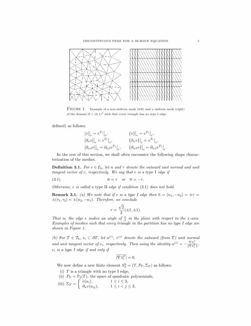
DISCONTINUOUS FEMS FOR A BI-WAVE EQUATION 5
Figure 1. Example of a non-uniform mesh (left) and a uniform mesh (right)
of the domain Ω = (0, 1)2 such that every triangle has no type I edge.
defined) as follows:
[v]∣∣e
= vT1∣∣e, v
∣∣e
= vT1∣∣e,
[∂αv]∣∣e
= vT1∣∣e, ∂αv
∣∣e
= vT1∣∣e,
[∂αβv]∣∣e
= ∂αβvT1∣∣e, ∂αβv
∣∣e
= ∂αβvT1∣∣e.
In the rest of this section, we shall often encounter the following shape charac-terization of the meshes.
Definition 3.1. For e ∈ Eh, let n and τ denote the outward unit normal and unittangent vector of e, respectively. We say that e is a type I edge if
n = τ or n = −τ.(3.1)
Otherwise, e is called a type II edge if condition (3.1) does not hold.
Remark 3.1. (a) We note that if e is a type I edge then n = (n1,−n2) = ±τ =±(τ1, τ2) = ±(n2,−n1). Therefore, we conclude
τ =√
22
(±1,±1).
That is, the edge e makes an angle of π4 in the plane with respect to the x-axis.
Examples of meshes such that every triangle in the partition has no type I edge areshown in Figure 1.
(b) For T ∈ Th, ei ⊂ ∂T , let n(i), τ (i) denote the outward (from T ) unit normaland unit tangent vector of ei, respectively. Then using the identity n(i) = − ∇λT
i
‖∇λTi ‖
,ei is a type I edge if and only if
|∇λTi | = 0.
We now define a new finite element Sh2 = (T, PT ,ΣT ) as follows:(i) T is a triangle with no type I edge,(ii) PT = P2(T ), the space of quadratic polynomials,
(iii) ΣT =v(ai), 1 ≤ i ≤ 3,∂nv(aij), 1 ≤ i < j ≤ 3,
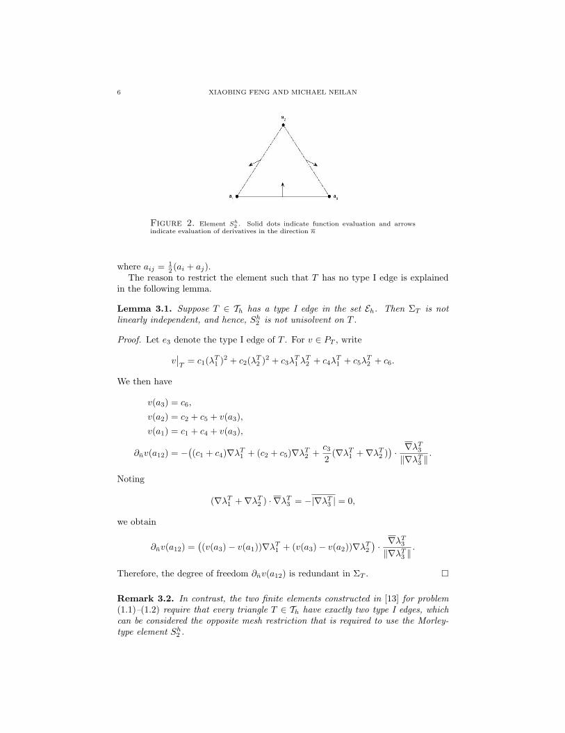
6 XIAOBING FENG AND MICHAEL NEILAN
Figure 2. Element Sh2 . Solid dots indicate function evaluation and arrows
indicate evaluation of derivatives in the direction n
where aij = 12 (ai + aj).
The reason to restrict the element such that T has no type I edge is explainedin the following lemma.
Lemma 3.1. Suppose T ∈ Th has a type I edge in the set Eh. Then ΣT is notlinearly independent, and hence, Sh2 is not unisolvent on T .
Proof. Let e3 denote the type I edge of T . For v ∈ PT , write
v∣∣T
= c1(λT1 )2 + c2(λT2 )2 + c3λT1 λ
T2 + c4λ
T1 + c5λ
T2 + c6.
We then have
v(a3) = c6,
v(a2) = c2 + c5 + v(a3),
v(a1) = c1 + c4 + v(a3),
∂nv(a12) = −((c1 + c4)∇λT1 + (c2 + c5)∇λT2 +
c32
(∇λT1 +∇λT2 ))· ∇λ
T3
‖∇λT3 ‖.
Noting
(∇λT1 +∇λT2 ) · ∇λT3 = −|∇λT3 | = 0,
we obtain
∂nv(a12) =((v(a3)− v(a1))∇λT1 + (v(a3)− v(a2))∇λT2
)· ∇λ
T3
‖∇λT3 ‖.
Therefore, the degree of freedom ∂nv(a12) is redundant in ΣT .
Remark 3.2. In contrast, the two finite elements constructed in [13] for problem(1.1)–(1.2) require that every triangle T ∈ Th have exactly two type I edges, whichcan be considered the opposite mesh restriction that is required to use the Morley-type element Sh2 .
DISCONTINUOUS FEMS FOR A BI-WAVE EQUATION 7
Remark 3.3. The basis functions associated with the element Sh2 = (T, PT ,ΣT )are given by
ϕTj : =‖∇λTj ‖|∇λTj |
λTj (λTj − 1), 1 ≤ j ≤ 3,
ϕTij : = 1− (λTi + λTj ) + 2λTi λTj
−∇λTi · ∇λTj( ϕTi‖∇λTi ‖
+ϕTj‖∇λTj ‖
), 1 ≤ i < j ≤ 3.
We note that if we replace ∇(·) with ∇(·) and |∇(·)| with ‖∇(·)‖2, we obtain thestandard basis functions for the Morley element [17, 22].
3.2. Properties of the new finite element. Let V h be the corresponding finiteelement space to the element Sh2 , and let V h0 consist of the functions in V h whosedegrees of freedom vanish on ∂Ω, that is,
V h =v∣∣T∈ P2(T ); v is continuous at each degree of freedom in ΣT , ∀T ∈ Th
,
V h0 =v ∈ V h; v vanishes at all degrees of freedom on ∂Ω
.
Next, define the following broken Sobolev norms and semi-norms
‖v‖2m,h :=∑T∈Th
‖v‖2Hm(T ), |v|2m,h :=∑T∈Th
|v|2Hm(T ),
and it is understood that ‖v‖0,h = ‖v‖L2 .Let ΠT v denote the standard interpolation of v associated with the finite element
Sh2 , that is,
ΠT v =∑
1≤i<j≤3,k 6=i,j
ϕTijv(ak) +3∑j=1
ϕTj ∂nv(aj).
We also define Πhv ∈ V h such that Πhv∣∣T
= ΠT
(v∣∣T
), ∀T ∈ Th. We note that
ΠT v = v ∀v ∈ P2(T ), and therefore, using standard interpolation theory [7] wehave for 0 ≤ m ≤ 3
|v −ΠT v|Hm(T ) ≤ Ch3−m|v|H3(T ) ∀v ∈ H3(T ), T ∈ Th.
Next, we show that the finite element space V h inherits a form of ‘weak conti-nuity’ which will play a crucial role in our analysis.
Lemma 3.2. For all α ∈ R2∫e
[∂αv]ds = 0 ∀v ∈ V h, e ∈ EIh,∫e
∂αvds = 0 ∀v ∈ V h0 , e ∈ EBh .
Proof. Given e ∈ Eh, let a1, a2 denote the endpoints of e, a12 the midpoint of e,and n, τ the normal and tangential direction of e. By hypothesis n 6= ±τ . Thus,

8 XIAOBING FENG AND MICHAEL NEILAN
we can write for any constant vector α ∈ R2,∫e
∂αvds =1
1− (τ · n)2
∫e
(α ·(τ − n(τ · n)
)∂τv + α ·
(n− τ(τ · n)
)∂nv
)ds
=1
1− (τ · n)2
(α ·(τ − n(τ · n)
)(v(a2)− v(a1))
+ α ·(n− τ(τ · n)
)∂nv(a12)
).
¿From this identity, the desired result follows.
¿From the above ‘weak continuity’ result, we get the following lemmas (see [22]).
Lemma 3.3. Let e ∈ Eh. Then if e = ∂T1 ∩ ∂T2 for some T1, T2 ∈ Th,
‖[v]‖L2(e) + h ‖[∇v]‖L2(e) ≤ Ch32(|v|H2(T1) + |v|H2(T2)
)∀v ∈ V h,
and if e = ∂T1 ∩ ∂Ω for some T1 ∈ Th,
‖[v]‖L2(e) + h ‖[∇v]‖L2(e) ≤ Ch32 |v|H2(T1) ∀v ∈ V h0 .
Lemma 3.4. For every v ∈ V h0 , there exists functions vk ∈ H10 (Ω) k = 0, 1, 2 with
vk∣∣T∈ P1(T ) such that
|v − v0|m,h ≤ Ch2−m|v|2,h 0 ≤ m ≤ 2,∣∣∂xkv − vk
∣∣m,h≤ Ch1−m|v|2,h 0 ≤ m ≤ 1, k = 1, 2.
Corollary 3.1. | · |m,h and ‖ · ‖m,h are equivalent on V h0 for m = 0, 1, 2.
Proof. Using the inverse inequality and Poincare’s inequality, we have
‖v‖L2 ≤ ‖v0‖L2 + ‖v − v0‖L2 ≤ |v0|H1 + Ch2|v|2,h≤ C|v|1,h + Ch|v|1,h ≤ C|v|1,h ∀v ∈ V h0 .
Similarly, for k = 1, 2
‖∂xkv‖L2 ≤ ‖vk‖L2 + ‖∂xk
v − vk‖L2 ≤ |vk|H1 + Ch|v|2,h ≤ C|v|2,h.
¿From these two identities, the desired results follow.
3.3. Formulation and convergence analysis of the Morley-type noncon-forming method. Based on (2.1), we define our nonconforming finite elementmethod as seeking uh ∈ V h0 such that
Aδh(uh, v) = (f, v) ∀v ∈ V h0 ,(3.2)
where
Aδh(v, w) =∑T∈Th
(δ(v,w)T + (∇v,∇w)T
)+∑e∈Eh
γh| lnh|(⟨
[∂τ τv], [∂τ τw]⟩e
+ 〈[∂τ nv], [∂τ nw]〉e).
Recall that τ = (τ1, τ2) and n = (n1, n2) denote the unit tangent and outward unitnormal to e, τ := (τ1,−τ2) = (n2, n1), and he = |e|, the length of e. Also, (·, ·)T

DISCONTINUOUS FEMS FOR A BI-WAVE EQUATION 9
and 〈·, ·〉e denote the L2 inner product on T and e, respectively. We note thatAδh(·, ·) induces the following energy norm on V h0 :
‖v‖2M :=∑T∈Th
(δ‖v‖2L2(T ) + ‖∇v‖2L2(T )
)(3.3)
+∑e∈Eh
γh| lnh|(‖[∂τ τv]‖2L2(e) + ‖[∂τ nv]‖2L2(e)
).
Remark 3.4. In the finite element method (3.2), the jump terms are the so-calledpenalty terms. The reason to include penalty terms into the finite element methodis to ensure that ‖ · ‖M is equivalent (independent of h) to the broken Sobolev norm‖ · ‖2,h on the space V h0 (see Lemma 3.6). We note that the basis functions ϕTijsatisfy (cf. Remark 3.3)
ϕTij = 0 ∀T ∈ Th, 1 ≤ i < j ≤ 3.
Therefore equivalence of ‖ · ‖M and ‖ · ‖2,h cannot be obtained in the absence ofpenalty terms.
For clarity of the presentation, we also introduce the following additional nota-tion:
ST (v, w) := 〈∂τ τv, ∂nw〉∂T − 〈∂τ nv, ∂τw〉∂T ,QT (v, w) := 2(∂xyv, ∂xyw)T + (∂xxv, ∂yyw)T + (∂yyv, ∂xxw)T ,
S(v, w) :=∑T∈Th
ST (v, w),
Q(v, w) :=∑T∈Th
QT (v, w).
Before proving the main results of this section, we first establish two technicallemmas.
Lemma 3.5. For any T ∈ Th and any two smooth functions v and w on T , thereholds the following identity:
ST (v, w) = 〈∂xyv, ∂xwn2〉∂T + 〈∂xyv, ∂ywn1〉∂T+ 〈∂yyv, ∂xwn1〉∂T + 〈∂xxv, ∂ywn2〉∂T .
Proof. By definition, we have
ST (v, w) =⟨∂τ τv, ∂nw
⟩∂T−⟨∂τ nv, ∂τw
⟩∂T
=⟨∂xxv τ
21 + 2∂xyv τ1τ2 + ∂yyv τ
22 , ∂xwn1 + ∂ywn2
⟩∂T−⟨∂xxv τ1n1
+ ∂xyv n1τ2 + ∂xyv τ1n2 + ∂yyv τ2n2, ∂xw τ1 + ∂yw τ2⟩∂T.
Since (n1, n2) = (n1,−n2) and (τ1, τ2) = (n2, n1),
ST (v, w) =⟨∂xxv n
22 + 2∂xyv n1n2 + ∂yyv n
21, ∂xwn1 + ∂ywn2
⟩∂T
−⟨∂xxv n1n2 + ∂xyv n
21 − ∂xyv n2
2 − ∂yyv n2n1, ∂xwn2 − ∂ywn1
⟩∂T.
10 XIAOBING FENG AND MICHAEL NEILAN
Finally, expanding the last expression and grouping similar terms, we conclude
ST (v, w) =⟨∂xw, ∂xxv n
22n1 + 2∂xyv n2
1n2 + ∂yyv n31 − ∂xxv n1n
22
⟩∂T
+ 〈∂xw, ∂xyv n32 − ∂xyv n2
1n2 + ∂yyv n1n22〉∂T
+ 〈∂yw, ∂xxv n32 + 2∂xyv n1n
22 + ∂yyv n
21n2 + ∂xxv n
21n2〉∂T
+ 〈∂yw, ∂xyv n31 − ∂xyv n2
2n1 − ∂yyv n2n21〉∂T
=⟨∂xw, ∂xyv n2(n2
1 + n22) + ∂yyv n1(n2
1 + n22)⟩∂T
+ 〈∂yw, ∂xxv n2(n21 + n2
2) + ∂xyv n1(n21 + n2
2)〉∂T=⟨∂xyv, ∂xwn2〉∂T + 〈∂xyv, ∂ywn1
⟩∂T
+ 〈∂xxv, ∂ywn2〉∂T + 〈∂yyv, ∂xwn1〉∂T .
Corollary 3.2. For any T ∈ Th, v, w ∈ P2(T ), there holds the following identity:
QT (v, w) = ST (v, w)
Proof. Since v, w∣∣T∈ P2(T ), integrating by parts and applying Lemma 3.5 gives us
QT (v, w) =⟨∂xyv, ∂xwn2
⟩∂T
+⟨∂xyv, ∂ywn1
⟩∂T
+⟨∂yyv, ∂xwn1
⟩∂T
+⟨∂xxv, ∂ywn2
⟩∂T
= ST (v, w).
Lemma 3.6. There exists a γ0 = O(δ) such that for γ ≥ γ0 there holds the followinginequality
‖v‖2M ≥ δC‖v‖22,h ∀v ∈ V h0 ,(3.4)
where C is a positive constant independent of γ and h.
Proof. We divide the proof into three steps.
Step 1: Integrating by parts and applying Corollary 3.2 yield
‖v‖2M =∑T∈Th
(δ‖v‖2T + ‖∇v‖2T
)+∑e∈Eh
γh| lnh|(‖[∂τ τv]‖2L2(e) + ‖[∂τ nv]‖2L2(e)
)=∑T∈Th
(δ‖D2v‖2L2(T ) + ‖∇v‖2L2(T ) − δQT (v, v)
)+∑e∈Eh
γh| lnh|(‖[∂τ τv]‖2L2(e) + ‖[∂τ nv]‖2L2(e)
)=∑T∈Th
(δ‖D2v‖2L2(T ) + ‖∇v‖2L2(T ) − δST (v, v)
)+∑e∈Eh
γh| lnh|(‖[∂τ τv]‖2L2(e) + ‖[∂τ nv]‖2L2(e)
).
DISCONTINUOUS FEMS FOR A BI-WAVE EQUATION 11
Hence, by Lemma 3.2,
‖v‖2M =∑T∈Th
(δ‖D2v‖2T + ‖∇v‖2L2(T )
)+∑e∈Eh
(γh| lnh|
(‖[∂τ τv]‖2L2(e)(3.5)
+ ‖[∂τ nv]‖2L2(e)
)− δ(⟨
[∂τ τv], ∂nv⟩
+⟨∂τ τv, [∂nv]
⟩e
−⟨[∂τ nv], ∂τv
⟩e−⟨∂τ nv, [∂τv]
⟩e
))=∑T∈Th
(δ‖D2v‖2L2(T ) + ‖∇v‖2L2(T )
)+∑e∈Eh
(γh| lnh|
(‖[∂τ τv]‖2L2(e)
+ ‖[∂τ nv]‖2L2(e)
)− δ(⟨
[∂τ τv], ∂nv⟩e−⟨[∂τ nv], ∂τv
⟩e
))≥∑T∈Th
(δ‖D2v‖2L2(T ) + ‖∇v‖2L2(T )
)+∑e∈Eh
(γh| lnh|
(‖[∂τ τv]‖2L2(e)
+ ‖[∂τ nv]‖2L2(e)
)− δ(∣∣⟨[∂τ τv], ∂nv
⟩e
∣∣+∣∣⟨[∂τ nv], ∂τv
⟩e
∣∣)).Step 2: Next, we derive a lower bound for each of the last two terms on the
right-hand side of (3.5). Since v is quadratic, both ∂τ τv and ∂τ nv are constantsalong each e ∈ Eh. By Lemma 3.2 we have
⟨[∂τ τv], ∂nv
⟩e
=⟨[∂τ τv], ∂nv+
12
[∂nv]⟩e
=⟨[∂τ τv], ∂nv
⟩e,⟨
[∂τ nv], ∂τv⟩e
=⟨[∂τ nv], ∂τv+
12
[∂τv]⟩e
=⟨[∂τ nv], ∂τv
⟩e.
Let e1 = (1, 0)T and e2 = (0, 1)T denote the canonical orthogonal basis for R2.For e ∈ Eh, let T ∈ Th be the element (with larger global labeling) which has eas its one edge. On noting that [∂τ τv] and [∂τ nv] are constants along e, by thequasiuniformity of Th we get
∣∣⟨[∂ τ τv], ∂nv⟩e
∣∣≤ Che ‖[∂τ τv]‖L∞(e) ‖∇v‖L∞(T )(3.6)
≤ Che ‖[∂τ τv]‖L∞(e)
(‖∂e1v‖L∞(T ) + ‖∂e2v‖L∞(T )
)≤ h| lnh|
2ε‖[∂τ τv]‖2L2(e) + C
ε
| lnh|
(‖∂e1v‖2L∞(T ) + ‖∂e2v‖2L∞(T )
),∣∣⟨[∂ τ nv], ∂nv
⟩e
∣∣≤ Che ‖[∂τ nv]‖L∞(e) ‖∇v‖L∞(T )(3.7)
≤ Che ‖[∂τ nv]‖L∞(e)
(‖∂e1v‖L∞(T ) + ‖∂e2v‖L∞(T )
)≤ h| lnh|
2ε‖[∂τ nv]‖2L2(e) + C
ε
| lnh|
(‖∂e1v‖2L∞(T ) + ‖∂e2v‖2L∞(T )
).
where ε is a positive number to be chosen later.To continue, we use a discrete Sobolev-Poincare inequality for piecewise polyno-
mials, which was proved in [5] (also see [16] for a related inequality for piecewise
12 XIAOBING FENG AND MICHAEL NEILAN
H1 functions), to get∑T∈Th
‖∂eiv‖2L∞(T ) ≤ C | lnh|
[∑T∈Th
‖D2v‖2L2(T )(3.8)
+∑e∈Eh
h−1e ‖Pe0 [∂ei
v]‖2L2(e)
]for i = 1, 2,
where C > 0 is an h-independent constant, and Pe0 denotes the constant projectionof L2(e) onto P0(e).
In view of Lemma 3.2 and the definition of V h0 , we have
Pe0 [∂eiv] = 0 ∀v ∈ V h0 , ∀e ∈ Eh, i = 1, 2.
Hence, by (3.8) we get∑T∈Th
‖∂eiv‖2L∞(T ) ≤ C | lnh|
∑T∈Th
‖D2v‖2L2(T ) for i = 1, 2.
Now, summing over all edges after adding (3.6) and (3.7), we obtain∑e∈Eh
(∣∣⟨[∂τ τv], ∂nv⟩e
∣∣+∣∣⟨[∂τ nv], ∂τv
⟩e
∣∣)(3.9)
≤ h| lnh|ε
∑e∈Eh
(∥∥[∂τ τv]∥∥2
L2(e)+∥∥[∂τ nv]
∥∥2
L2(e)
)+ εC
∑T∈Th
‖D2v‖2L2(T ).
Step 3: Combining (3.5) and (3.9) gives us
‖v‖2M ≥∑T∈Th
(δ(1− εC)‖D2v‖2L2(T ) + ‖∇v‖2L2(T )
)+ h| lnh|
(γ − δ
ε
) ∑e∈Eh
(‖[∂τ τv]‖2L2(e) + ‖[∂τ nv]‖2L2(e)
).
Choosing ε = 12C , γ0 = 2δC, we obtain for γ ≥ γ0
‖v‖2M ≥∑T∈Th
(δ2‖D2v‖2L2(T ) + ‖∇v‖2L2(T )
)≥ Cδ‖v‖22,h.
The proof is complete.
With Lemma 3.6 in hand, we are now able to show the first main result of thissection.
Theorem 3.1. There exists a unique solution uh to (3.2). Furthermore, if u ∈H3(Ω) and γ ≥ γ0, the following error estimates hold:
‖u− uh‖M ≤ h(C1‖f‖L2 + C2‖u‖H3
),(3.10)
‖u− uh‖2,h ≤Ch√δ
(C1‖f‖L2 + C2‖u‖H3
),(3.11)
where
C1 =CM0√δ, C2 = C
√δ + h2 + γ| lnh|.

DISCONTINUOUS FEMS FOR A BI-WAVE EQUATION 13
Proof. Since problem (3.2) is linear and in a finite dimensional setting, it sufficesto show uniqueness. Thus, suppose w ∈ V h0 satisfies
Aδh(w, v) = 0 ∀v ∈ V h0 .
It follows that w is piecewise constant on each T ∈ Th. By Corollary 3.1, weconclude 0 = |w|1,h ≥ C‖w‖1,h, and hence w ≡ 0.
To show the error estimate (3.10), we use Strang’s second lemma [7, 6] to get
‖u− uh‖M ≤ infv∈V h
0
‖u− v‖M + sup0 6=v∈V h
0
∣∣Aδh(u, v)− (f, v)∣∣
‖v‖M.(3.12)
Using Lemma 3.4 (v0 is defined there),
(f, v) = (δ2u−∆u, v0) + (f, v − v0)
= (−δ∇u+∇u,∇v0) + (f, v − v0)
=∑T∈Th
(δ(u,v)T + (∇u,∇v)T + (−δ∇u+∇u,∇(v0 − v))T
− δ⟨u, ∂nv
⟩∂T
)+ (f, v − v0)
=∑T∈Th
(δ(u,v)T + (∇u,∇v)T + (−δ∇u+∇u,∇(v0 − v))T
)− δ
∑e∈Eh
⟨u, [∂nv]
⟩e
+ (f, v − v0)
= Aδh(u, v) +∑T∈Th
(−δ∇u+∇u,∇(v0 − v))T
− δ∑e∈Eh
⟨u, [∂nv]
⟩e
+ (f, v − v0).
Next, by Lemma 3.2, we have
δ∣∣∣∑e∈Eh
⟨u, [∂nv]
⟩e
∣∣∣ = δ∣∣∣∑e∈Eh
⟨u− Pe0u, [∂nv]− Pe0 [∂nv]
⟩e
∣∣∣≤ δCh‖∇u‖L2‖v‖2,h.
Also, ∣∣∣δ ∑T∈Th
(∇u,∇(v0 − v)
)T
∣∣∣ =∣∣∣δ ∑T∈Th
(∇u,∇(v0 − v)
)T
∣∣∣≤ δCh‖∇u‖L2‖v‖2,h,
and by Lemma 3.4∣∣∣ ∑T∈Th
(∇u,∇(v0 − v)
)T
+ (f, v − v0)∣∣∣
=∣∣∣ ∑T∈Th
(∆u, v − v0
)T−∑e∈Eh
〈∂nu, [v]〉e + (f, v − v0)∣∣∣
≤ C(h
32 ‖∆u‖L2 + h2‖f‖L2
)‖v‖2,h +
∑e∈Eh
‖∂nu‖L2(e)‖[v]‖L2(e).
14 XIAOBING FENG AND MICHAEL NEILAN
By the Cauchy-Schwarz inequality, the trace/inverse inequality
‖∂nu‖L2(e) ≤ Ch−12 ‖u‖H2(T )
(assuming e is an edge of the element T , see (iii) of Lemma 2.1), and Lemma 3.3we get∑
e∈Eh
‖∂nu‖L2(e)‖[v]‖L2(e) ≤(∑e∈Eh
‖∂nu‖2L2(e)
) 12(∑e∈Eh
‖[v]‖2L2(e)
) 12
≤ C(∑T∈Th
h−1‖u‖2H2(T )
) 12(∑T∈Th
h3‖v‖2H2(T )
) 12
≤ Ch‖u‖H2 ‖v‖2,h≤ Ch‖∆u‖L2 ‖v‖2,h.
Using these inequalities, the regularity result (2.3), and Lemma 3.6 it followsthat ∣∣Aδh(u, v)− (f, v)
∣∣ ≤ Ch(δ‖∇u‖L2 + ‖∆u‖L2 + h‖f‖L2
)‖v‖2,h,(3.13)
≤ Ch(√
δM0 +M0 + h)‖f‖L2‖v‖2,h
≤ CM0h‖f‖L2‖v‖2,h
≤ CM0h√δ‖f‖L2‖v‖M .
Next, appealing to the inverse and trace inequalities, we have
‖u−Πhu‖2M =∑T∈Th
(δ‖(u−Πhu)‖2L2(T ) + ‖∇(u−Πhu)‖2L2(T )
)+∑e∈Eh
γh| lnh|(‖[∂τ τ (u−Πhu)]‖2L2(e) + ‖[∂τ n(u−Πhu)]‖2L2(e)
)≤ Ch2(δ + h2 + γ| lnh|)‖u‖2H3 .
Thus,
infv∈V h
0
‖u− v‖M ≤ Ch√δ + h2 + γ| lnh| ‖u‖H3 .(3.14)
Combining (3.12)–(3.14), we obtain
‖u− uh‖M ≤ Ch(M0√δ‖f‖L2 +
√δ + h2 + γ| lnh| ‖u‖H3
)≤ h
(C1‖f‖L2 + C2‖u‖H3
).
To prove (3.11), we use the triangle inequality and Lemma 3.6
‖u− uh‖2,h ≤ ‖u−Πhu‖2,h + ‖Πhu− uh‖2,h
≤ Ch‖u‖H3 +C√δ‖Πhu− uh‖M
≤ Ch‖u‖H3 +C√δ
(‖u−Πhu‖M + ‖u− uh‖M
)≤ Ch√
δ
(C1‖f‖L2 + C2‖u‖H3
).
DISCONTINUOUS FEMS FOR A BI-WAVE EQUATION 15
The second main theorem of this section, which is stated below, concerns theH1-norm error estimate for the proposed Morley-type nonconforming method.
Theorem 3.2. In addition to the hypotheses of Theorem 3.1, assume Ω is convex.Then the following estimate holds:
‖u− uh‖1,h ≤ h2(C3‖f‖L2 + C4‖u‖H3
),(3.15)
where
C3 = C3(γ, δ, h, CE) = CCE
(1 + C2
2 +C2(1 + δ| lnh|)√
δ
),
C4 = C4(γ, δ, h, CE) = CCE
(h+ C1C2 +
C1(1 + δ| lnh|)√δ
).
and CE is defined by (3.19).
Proof. The proof is quite technical, so we break it up into four steps.
Step 1: A duality argument
Let eh = u− uh, ρh = Πheh = Πhu− uh ∈ V h0 and ρ0 ∈ H10 (Ω) be as defined in
Lemma 3.4. First, we state the following stability estimates:
‖ρh‖2,h ≤ ‖eh‖2,h + ‖u−Πhu‖2,h ≤ C‖eh‖2,h,(3.16)
|ρh|1,h ≤ |ρh − ρ0|1,h + ‖∇ρ0‖L2(3.17)
≤ h‖ρh‖2,h + ‖∇ρ0‖L2 ≤ Ch‖eh‖2,h + ‖∇ρ0‖L2 ,
‖∇ρ0‖L2 ≤ |ρh|1,h + |ρ0 − ρh|1,h(3.18)
≤ |ρh|1,h + Ch|ρh|2,h ≤ C|ρh|1,h.
Next, let ϕ ∈ H3(Ω)∩H20 (Ω) be the solution to the following auxiliary problem:
δ∆2ϕ−∆ϕ = −∆ρ0 in Ω,ϕ = ∂nϕ = 0 on ∂Ω.
Since ρ0 ∈ H10 (Ω) and Ω is convex, it follows from standard elliptic theory [9] that
‖ϕ‖H3 ≤ CE‖∇ρ0‖L2 .(3.19)
Integrating by parts, we obtain
‖∇ρ0‖2L2 = (−δ∇∆ϕ+∇ϕ,∇ρ0)
=∑T∈Th
((−δ∇∆ϕ+∇ϕ,∇ρh)T + (−δ∇∆ϕ+∇ϕ,∇(ρ0 − ρh))T
)=∑T∈Th
(δ(D2ϕ,D2ρh)T + (∇ϕ,∇ρh)T + (−δ∇∆ϕ+∇ϕ,∇(ρ0 − ρh))T
)− δ
∑e∈Eh
(〈∆ϕ− ∂ττϕ, [∂nρh]〉e + 〈∂nτϕ, [∂τρh]〉e
).
Applying Corollary 3.2 yields
(D2ϕ,D2ρh)T = (ϕ,ρh)T +QT (Πhϕ, ρh) +QT (ϕ−Πhϕ, ρh)
= (ϕ,ρh)T + ST (ϕ, ρh) + ST (Πhϕ− ϕ, ρh) +QT (ϕ−Πhϕ, ρh),
16 XIAOBING FENG AND MICHAEL NEILAN
and hence, we obtain the following identity
‖∇ρ0‖2L2 = Aδh(ϕ, ρh) +∑T∈Th
(−δ∇∆ϕ+∇ϕ,∇(ρ0 − ρh))T(3.20)
− δ∑e∈Eh
(〈∆ϕ− ∂ττϕ, [∂nρh]〉e + 〈∂nτϕ, [∂τρh]〉e
)+ δ(S(ϕ, ρh) + S(Πhϕ− ϕ, ρh) +Q(ϕ−Πhϕ, ρh)
).
Step 2: Bounding the last six terms in (3.20).
First, using standard interpolation results and (3.16) we get
Q(ϕ−Πhϕ, ρh) ≤ C|ϕ−Πhϕ|2,h|ρh|2,h ≤ Ch‖ϕ‖H3‖eh‖2,h.(3.21)
Next, using the trace inequality we have for any T ∈ ThST (Πhϕ− ϕ, ρh) =
⟨∂τ τ (Πhϕ− ϕ), ∂nρh
⟩∂T−⟨∂τ n(Πhϕ− ϕ), ∂τρh
⟩∂T
≤ ‖∂τ τ (Πhϕ− ϕ)‖L2(∂T )‖∂nρh‖L2(∂T )
+ ‖∂τ n(Πhϕ− ϕ)‖L2(∂T )‖∂τρh‖L2(∂T )
≤ Ch 12 ‖ϕ‖H3(T )‖∇ρh‖L2(∂T )
≤ Ch‖ϕ‖H3(T )‖∇ρh‖L∞(T ).
Therefore, using (3.17) and a similar technique as that found in Step 2 of theproof of Lemma 3.6, we have
S(Πhϕ− ϕ, ρh) =∑T∈Th
ST (Πhϕ− ϕ, ρh)(3.22)
≤ Ch| lnh|‖ϕ‖H3‖ρh‖2,h≤ Ch| lnh|‖ϕ‖H3‖eh‖2,h.
Next, using Lemma 3.2 and (3.16)
S(ϕ, ρh) =∑e∈Eh
(〈∂τ τϕ, [∂nρh]〉e − 〈∂τ nϕ, [∂τρh]〉e
)(3.23)
=∑e∈Eh
(〈∂τ τϕ− Pe0 (∂τ τϕ) , [∂nρh]− Pe0 ([∂nρh])〉e
− 〈∂τ nϕ− Pe0 (∂τ nϕ) , [∂τρh]− Pe0 ([∂τρh])〉e)
≤ Ch‖ϕ‖H3‖ρh‖2,h≤ Ch‖ϕ‖H3‖eh‖2,h,
Similarly, we conclude∑e∈Eh
(〈∆ϕ− ∂ττϕ, [∂nρh]〉e + 〈∂nτϕ, [∂τρh]〉e
)≤ Ch‖ϕ‖H3‖eh‖2,h,(3.24)
and using Lemma 3.4, we obtain∑T∈Th
(−δ∇∆ϕ+∇ϕ,∇(ρ0 − ρh))T ≤ C‖ϕ‖H3‖ρ0 − ρh‖1,h(3.25)
≤ Ch‖ϕ‖H3‖eh‖2,h.

DISCONTINUOUS FEMS FOR A BI-WAVE EQUATION 17
Applying bounds (3.21)–(3.25) to (3.20), we have
‖∇ρ0‖2L2 ≤ Aδh(ϕ, ρh) + Ch(1 + δ| lnh|)‖eh‖2,h‖ϕ‖H3 .(3.26)
Step 3: Bounding Aδh(ϕ, ρh)
To bound Aδh(ϕ, ρh), we write
Aδh(ϕ, ρh) = Aδh(eh, ϕ−Πhϕ) +Aδh(eh,Πhϕ) +Aδh(ϕ,Πhu− u).(3.27)
Bounding the third term in (3.27)
Aδh(ϕ,Πhu− u) =∑T∈Th
(δ(ϕ,(Πhu− u))T + (∇ϕ,∇(Πhu− u))T
)=∑T∈Th
(−δ(∇ϕ,∇(Πhu− u)
)T
+(∇ϕ,∇(Πhu− u)
)T
)(3.28)
+∑e∈Eh
δ⟨ϕ− Pe0 (ϕ) , [∂n(Πhu− u)]− Pe0 ([∂n(Πhu− u)])
⟩e
≤ Ch2‖ϕ‖H3‖u‖H3 .
To bound the second term in (3.27), we have
Aδh(eh,Πhϕ) = Aδh(u,Πhϕ)− (f, ϕ)− (f,Πhϕ− ϕ)
=∑T∈Th
(−δ∇u+∇u,∇(Πhϕ− ϕ))T − (f,Πhϕ− ϕ)(3.29)
+ δ∑e∈Eh
⟨u− Pe0(u), [∂n(Πhϕ− ϕ)]− Pe0 [∂n(Πhϕ− ϕ)]
⟩e
≤ Ch2(‖u‖H3 + h‖f‖L2)‖ϕ‖H3 .
We bound the first term in (3.27) as follows:
Aδh(eh, ϕ−Πhϕ) ≤ ‖eh‖M‖ϕ−Πhϕ‖M(3.30)
≤ CC2h‖ϕ‖H3‖eh‖M .
Combining (3.27)–(3.30), we obtain
Aδh(ϕ, ρh) ≤ Ch(h‖u‖H3 + h2‖f‖L2 + C2‖eh‖M
)‖ϕ‖H3 .(3.31)
Step 4: Finishing up
Using bounds (3.26) and (3.31), and the regularity result (3.19), we conclude
‖∇ρ0‖L2 ≤ CCE(h2‖u‖H3 + h3‖f‖L2 + C2h‖eh‖M + h(1 + δ| lnh|)‖eh‖2,h
)≤ CCEh2
[(1 + C2
2 +C2(1 + δ| lnh|)√
δ
)‖u‖H3
+(h+ C1C2 +
C1(1 + δ| lnh|)√δ
)‖f‖L2
].

18 XIAOBING FENG AND MICHAEL NEILAN
Finally, using the stability result (3.18), we have
|u− uh|1,h ≤ |u−Πhu|1,h + |ρh|1,h
≤ CCEh2
[(1 + C2
2 +C2(1 + δ| lnh|)√
δ
)‖u‖H3
+(h+ C1C2 +
C1(1 + δ| lnh|)√δ
)‖f‖L2
]≤ h2
(C3‖f‖L2 + C4‖u‖H3
).
The proof is complete.
We conclude this section by remarking that all results of this section are still validif the Morley-type nonconforming element Sh2 is replaced by the original Morleyelement (cf. [17, 20]) but making no change to the formulation of the method.
4. Interior penalty discontinuous Galerkin methods
In the previous section we constructed and analyzed a quadratic Morley-typenonconforming finite element method for problem (1.1)–(1.2). As in the case ofconforming finite elements [13], the construction of the Morley-type element is onlypossible on some special meshes (it is interesting to note that the mesh constraintsfor the conforming elements and for the nonconforming finite element are ‘orthogo-nal’ to each other). Moreover, in order to ensure the convergence of the Morley-typenonconforming finite element method, two (super)penalized jump terms must beintroduced in the mesh-dependent bilinear form Aδh(·, ·). These jump terms arenot only critically used in the convergence proof but also certified by numericalexperiments (see Section 5) to be indispensable for the convergence of the method.
To avoid the mesh constraints imposed by both conforming and nonconformingfinite element methods, and also considering the fact that interior penalty termsmust be used in the nonconforming method, it is natural to go one step further anddevelop interior penalty discontinuous Galerkin (DG) methods (cf. [10, 3, 23, 1]).This indeed is the main goal of this section.
In this section, we develop a family of interior penalty DG methods for problem(1.1)–(1.2). Our methods are closely related to the DG methods introduced byBaker [3] (also see [12]) for the biharmonic problem. As it is now well-known (cf.[2, 19] and the references therein), DG methods use trial and test spaces consistingof totally discontinuous polynomials, and as a result, the weak formulation naturallyinclude jump and average terms across element edges/faces, and penalty terms areintroduced to control the discontinuity between adjacent elements. DG methodsenjoy a number of advantages over (conforming and nonconforming) finite elementmethods. This is especially true for fourth-order problems such as (1.1)–(1.2) andthe biharmonic problem, which are difficult and delicate to solve by finite elementmethods.
4.1. Formulation of interior penalty DG methods. To formulate interiorpenalty DG methods for problem (1.1)–(1.2), we introduce some additional no-tation. Let Th be a locally quasiuniform triangulation of Ω with hT = diam(T ) andh = maxT∈Th
hT . Notation EIh, EBh , Eh, [v], and v are same as in Section 3. We

DISCONTINUOUS FEMS FOR A BI-WAVE EQUATION 19
also define
Whr =
∏T∈Th
Pr(T ), Whr = Wh
r ∩H10 (Ω), Hs(Th) =
∏T∈Th
Hs(T ),
where r ≥ 2 which will be assumed in the rest of this section.For T ∈ Th, it is easy to check the following Green’s identities hold for the
d’Alembertian and the bi-wave operator 2:∫T
v w dxdy =∫∂T
∂nv w ds−∫T
∇v · ∇w dxdy,∫T
2v w dxdy =∫∂T
(∂nv)w ds−∫∂T
v ∂nw ds+∫T
vw dxdy.
The second identity together with the elementary algebraic identity,
a+b+ − a−b− = [a]b+ a[b],motivates us to introduce the following mesh-dependent bilinear form on the prod-uct space H4(Th)×H4(Th):
aδh(v, w) : =∑T∈Th
(δ(v,w)T + (∇v,∇w)T
)+∑e∈Eh
(〈δ∂nv − ∂nv, [w]〉e
− δ 〈v, [∂nw]〉e + 〈δ∂nw − ∂nw, [v]〉e − δ 〈w, [∂nv]〉e+ γh−1
e 〈[∂nv], [∂nw]〉e + γh−3e 〈[v], [w]〉e
)∀v, w ∈ H4(Th).
As in the previous section, γ is a positive constant independent of h and the termsinvolving γ are the so-called penalty terms.
The bilinear form aδh(·, ·) induces the following norm on H4(Th):
‖v‖2E : =∑T∈Th
(δ‖v‖2L2(T ) + ‖∇v‖2L2(T )
)(4.1)
+∑e∈Eh
(γh−3
e ‖[v]‖2L2(e) + γh−1e ‖[∂nv]‖2L2(e)
+ δhe ‖v‖2L2(e) + δh3e ‖∂nv‖
2L2(e) + he ‖∂nv‖2L2(e)
).
We also define the following alternative norm which will be used later in the paper:
‖v‖2E
: =∑T∈Th
(δ‖v‖2L2(T ) + ‖∇v‖2L2(T )
)+∑e∈Eh
(γh−3
e ‖[v]‖2L2(e)(4.2)
+ γh−1e ‖[∂nv]‖2L2(e) + δhe ‖v‖2L2(e) + he ‖∂nv‖2L2(e)
).
We now define a weak formulation of (1.1)–(1.2) as seeking u ∈ H4(Th)∩V suchthat
aγh(u, v) = (f, v) ∀v ∈ H4(Th) ∩ V.(4.3)
Remark 4.1. One may easily verify that the formulation (4.3) is consistent. Thatis, if u ∈ H4(Ω)∩V is the solution to (1.1)–(1.2), then u satisfies (4.3). Conversely,if u ∈ H4(Ω) ∩ V0 solves (4.3) then u is the unique solution to (1.1)–(1.2).
Based on (4.3), we then define our interior penalty discontinuous Galerkin meth-ods as to find uh ∈Wh
r such that
aγh(uh, v) = (f, v) ∀v ∈Whr ,(4.4)
20 XIAOBING FENG AND MICHAEL NEILAN
We end this subsection by stating a lemma which concerns the approximationproperties of the finite element spaces Wh
r . We omit the proof to save space andrefer the reader to [3] for the proof of similar results.
Lemma 4.1. For any v ∈ Hs(Ω) (s ≥ 4), there exists v ∈Whr such that
‖v − v‖E ≤ C
(∑T∈Th
h2`−4T (δ + γ + h2
T )‖v‖2H`(T )
) 12
≤ Ch`−2(√γ + δ + h)‖v‖H` , r ≥ 3,
‖v − v‖E ≤ C
(∑T∈Th
h2T (δ + γ + h2
T )‖v‖2H4(T )
) 12
≤ Ch(√γ + δ + h)‖v‖H4 , r = 2.
Moreover, if v ∈ Hs(Ω) (s ≥ 3), there exists v ∈Whr such that
‖v − v‖E ≤ C
(∑T∈Th
h2`−4T (δ + γ + h2
T )‖v‖2H`(T )
) 12
≤ Ch`−2(√γ + δ + h)‖v‖H` , r ≥ 2.
Where ` = mins, r + 1.4.2. Convergence analysis of interior penalty DG methods. The followinglemma ensures that the bilinear form aγh(·, ·) is continuous and coercive on the finiteelement space Wh
r .
Lemma 4.2. There holds the following inequality:
|aδh(v, w)| ≤ 2‖v‖E‖w‖E ∀v, w ∈ H4(Th).(4.5)
Furthermore, there exists a positive constant γ0 = O(δ + h2) such that for γ ≥ γ0,there holds
aδh(v, v) ≥ C‖v‖2E ∀v ∈Whr .(4.6)
Proof. The proof is similar to the one found in [3, Propositions 5.1 and 5.2] (alsosee [19]). Clearly (4.5) is a direct consequence of the Cauchy-Schwarz inequality,so we only give a detailed proof of (4.6).
First, for v ∈Whr we have using the Cauchy-Schwarz and inverse inequalities
‖v‖2E ≤ C∑T∈Th
(δ‖v‖2L2(T ) + ‖∇v‖2L2(T )
)(4.7)
+ C∑e∈Eh
(γh−3
e ‖[v]‖2L2(e) + γh−1e ‖[∂nv]‖2L2(e)
).
Next, by definition we have
aγh(v, v) ≥∑T∈Th
(δ‖v‖2L2(T ) + ‖∇v‖2L2(T )
)(4.8)
+∑e∈Eh
(γh−3
e ‖[v]‖2L2(e) + γh−1e ‖[∂nv]‖2L2(e)
− 2∣∣⟨δ∂nv − ∂nv, [v]
⟩e
∣∣− 2δ∣∣⟨v, [∂nv]
⟩e
∣∣).

DISCONTINUOUS FEMS FOR A BI-WAVE EQUATION 21
Using the trace and inverse inequalities yields for e = T1 ∩ T2 ∈ EIh∣∣⟨∂nv, [v]⟩e
∣∣ ≤ C(‖v‖L2(T1) + ‖v‖L2(T2)
)h− 3
2e ‖[v]‖L2(e) ,∣∣⟨v, [∂nv]
⟩e
∣∣ ≤ C(‖v‖L2(T1) + ‖v‖L2(T2)
)h− 1
2e ‖[∂nv]‖L2(e) ,∣∣⟨∂nv, [v]
⟩e
∣∣ ≤ C(‖∇v‖L2(T1) + ‖∇v‖L2(T2)
)h− 1
2e ‖[v]‖L2(e) .
Similar inequalities hold on e ∈ EBh . Thus,
∑e∈Eh
δ∣∣⟨∂nv, [v]
⟩e
∣∣ ≤ δC (∑T∈Th
‖v‖2L2(T )
) 12(∑e∈Eh
h−3e ‖[v]‖2L2(e)
) 12
≤ δ
8
∑T∈Th
‖v‖2L2(T ) + δC∑e∈Eh
h−3e ‖[v]‖2L2(e) ,
∑e∈Eh
δ∣∣⟨v, [∂nv]
⟩e
∣∣ ≤ δC (∑T∈Th
‖v‖2L2(T )
) 12(∑e∈Eh
h−1e ‖[∂nv]‖2L2(e)
) 12
,
≤ δ
8
∑T∈Th
‖v‖2L2(T ) + δC∑e∈Eh
h−1e ‖[∂nv]‖2L2(e) ,
∑e∈Eh
∣∣⟨∂nv, [vh]⟩e
∣∣ ≤ C (∑T∈Th
‖∇v‖2L2(T )
) 12(∑e∈Eh
h−1e ‖[v]‖2L2(e)
) 12
≤ 14
∑T∈Th
‖∇v‖2L2(T ) + C∑e∈Eh
h−1e ‖[v]‖2L2(e) .
Combining these estimates with (4.8) we obtain
aδh(v, v) ≥ 12
∑T∈Th
(δ‖v‖2L2(T ) + ‖∇v‖2L2(T )
)+∑e∈Eh
(h−3e
(γ − C(δ + h2
e))‖[v]‖2L2(e)
+ h−1e
(γ − δC
)‖[∂nv]‖2L2(e)
).
Choosing γ0 = C(δ + h2) and using (4.7), we have for γ ≥ γ0
aδh(v, v) ≥ C‖v‖2E .
An immediate consequence of the above lemma is the following existence anduniqueness theorem.
Theorem 4.1. The discrete problem (4.4) has a unique solution for γ ≥ γ0.
We now are ready to state and prove one of the main theorems of this section.
Theorem 4.2. Let γ ≥ γ0 and suppose u ∈ Hs(Ω) (s ≥ 4) solves (1.1)–(1.2). Thenthere hold the following error estimates:
‖u− uh‖E ≤ Ch`−2(√γ + δ + h)‖u‖H` , r ≥ 3,(4.9)
‖u− uh‖E ≤ Ch(√γ + δ + h)‖u‖H4 , r = 2.(4.10)

22 XIAOBING FENG AND MICHAEL NEILAN
where ` = minr + 1, s, and C is independent of h, γ, and δ.
Proof. Using the consistency, coercivity, and continuity of the bilinear form aδh, wehave for γ ≥ γ0 and v ∈Wh
r
C‖uh − v‖2E ≤ aδh(uh − v, uh − v) = aδh(u− v, uh − v)
≤ 2‖u− v‖E‖uh − v‖E ,
and therefore
‖u− uh‖E ≤ ‖u− v‖E + ‖uh − v‖E ≤ C‖u− v‖E .
The error estimates (4.9)–(4.10) then follow directly from Lemma 4.1.
Next, we derive error estimates when the solution only belongs to H3(Ω). Tothe end, we need the following technical lemma which is concerned with how wella function in Wh
r can be approximated by continuous functions. A proof of thelemma can be found in [15].
Lemma 4.3. For any v ∈Whr , there exists Ehv ∈ Wh
r such that
‖v − Ehv‖2L2 ≤ C∑e∈EI
h
he ‖[v]‖2L2(e) +∑e∈EB
h
he‖v‖2L2(e),(4.11)
|v − Ehv|21,h ≤ C∑e∈EI
h
h−1e ‖[v]‖2L2(e) +
∑e∈EB
h
h−1e ‖v‖2L2(e).(4.12)
Theorem 4.3. Suppose u ∈ H3(Ω) is the unique solution to (1.1)–(1.2). Then forγ ≥ γ0, r = 2, there holds the following error estimate:
‖u− uh‖E ≤ Ch
(√γ + δ + h)‖u‖H3 +M0(
√δ + h)‖f‖L2
.(4.13)
Proof. We note that in the case r = 2, uh satisfies
aδh(uh, v) = (f, v) ∀v ∈Wh2 .
where
aδh(v, w) : =∑T∈Th
(δ(v,w)T + (∇v,∇w)T
)−∑e∈Eh
(〈∂nv, [w]〉e
+ δ 〈v, [∂nw]〉e + 〈∂nw, [v]〉e + δ 〈w, [∂nv]〉e− γh−1
e 〈[∂nv], [∂nw]〉e − γh−3e 〈[v], [w]〉e
).
We also have for γ ≥ γ0
aδh(v, v) = aδh(v, v) ≥ 12‖v‖E =
12‖v‖E ∀v ∈Wh
2 .
Since the bilinear form aδh(·, ·) is no longer consistent, we employ Strang’s SecondLemma to conclude
‖u− uh‖E ≤ C(
infv∈Wh
2
‖u− v‖E + sup06=v∈Wh
2
|aδh(u, v)− (f, v)|‖v‖E
).(4.14)

DISCONTINUOUS FEMS FOR A BI-WAVE EQUATION 23
To bound the last term in (4.14), we write
(f, v) = −δ(∇u,∇Ehv)− (∆u, v) + (f + ∆u, v − Ehv)
=∑T∈Th
(δ(u,v)T + (∇u,∇v)T − δ 〈u, ∂nv〉∂T − 〈∂nu, v〉∂T
− δ(∇u,∇(Ehv − v))T)
+ (f + ∆u, v − Ehv)
= aδh(u, v)− δ∑T∈Th
(∇u,∇(Ehv − v))T + (f + ∆u, v − Ehv).
Bounding the last two terms in the expression above, we use Lemma 4.3
δ∣∣∣ ∑T∈Th
(∇u,∇(Ehv − v))T∣∣∣ ≤ δC‖∇u‖L2
(∑e∈Eh
h−1e ‖[v]‖2L2(e)
) 12
≤ δCh‖∇u‖L2‖v‖E ,∣∣∣(f + ∆u, v − Ehv)∣∣∣ ≤ C(‖f‖L2 + ‖∆u‖L2)
(∑e∈Eh
he ‖[v]‖2L2(e)
) 12
≤ Ch2(‖f‖L2 + ‖∆u‖L2)‖v‖E .
Thus by (2.3),
supv∈Wh
2
∣∣aδh(u, v)− (f, v)∣∣
‖v‖E≤ Ch
(δ‖∇u‖L2 + h
(‖∆u‖L2 + ‖f‖L2
))(4.15)
≤ CM0h(√δ + h
)‖f‖L2 .
Next, it is clear from the proof of Lemma 4.1 that
infv∈Wh
r
‖u− v‖E ≤ Ch(√
γ + δ + h)‖u‖H3 .(4.16)
Combining (4.14)–(4.16), we obtain
‖u− uh‖E ≤ Ch
(√γ + δ + h)‖u‖H3 +M0(
√δ + h)‖f‖L2
.
Remark 4.2. Using a standard duality argument ([3, 13]) and the regularity es-timates (2.3), it is also possible to show the following L2-error estimates whenu ∈ H4(Ω):
‖u− uh‖L2 ≤ Ch`−1(√γ + δ + h)‖u‖H` , r ≥ 3,
‖u− uh‖L2 ≤ Ch2(√γ + δ + h)‖u‖H4 , r = 2.
5. Numerical Experiments
In this section, we provide numerical experiments to gauge the efficiency of thefinite element methods developed in the previous sections. We calculate the rate ofconvergence of ‖u − uh‖ for fixed δ in various norms and compare each computedrate with its theoretical estimate.

24 XIAOBING FENG AND MICHAEL NEILAN
Test 1. For this test, we solve (3.2) using the Morley-type nonconforming elementSh2 defined in Section 3 with Ω = (0, 1)2 and γ = δ. We use the following data:
f = −8π4δ(
cos2(πx)− sin2(πy))
− 2π2
sin2(πy)(
cos2(πx)− sin2(πx))
+ sin2(πx)(
cos2(πy)− sin2(πy)),
so that the exact solution is
u = sin2(πx) sin2(πy).
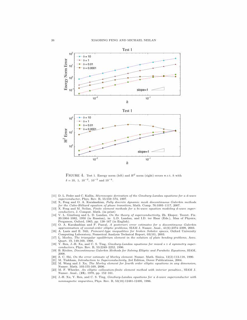
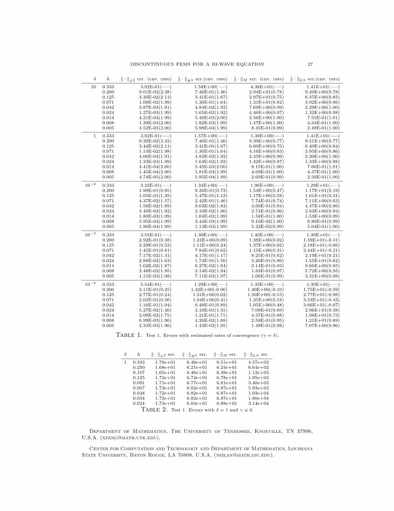
We list the errors along with their estimated rates of convergence in Table 1 forδ-values 10, 1, 10−2, 10−3, and 10−4 and plot the errors in Figures 3–4. The tableindicate the following rates of convergence:
‖u− uh‖M = O(h), ‖u− uh‖2,h = O(h),
‖u− uh‖1,h = O(h2), ‖u− uh‖L2 = O(h2).
Ignoring the insignificant | lnh| terms in (3.10)–(3.11), (3.15), these are the samerates of convergence established in Theorems 3.1 and 3.2. We also observe that asδ → 0+, the error increases in the L2, H1, and H2 norms which is expected by thedefinition of the constants in the error estimates (3.11) and (3.15).
Finally, we solve (3.2) but with γ ≡ 0 and δ = 1. Table 2 clearly shows thatthe method does not converge, this then indicates that the penalty terms in themethod are essential.
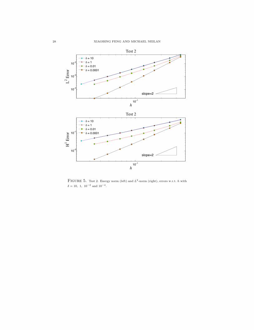
Test 2. In this test, we compute the solution of the discontinuous Galerkin method(4.4) with r = 2 and γ = 100δ. We use the same domain and test functions as inTest 1. We list the errors in Table 3 and plot the computed errors in Figures 5 and6 for δ−values 10, 1, 10−2, and 10−4. As expected, the rates of convergence dependon both the parameters h and δ. In fact, Theorem 4.2 and Remark 4.2 tells us thatfor√δ >> h, γ ≈ δ
‖u− uh‖E ≤ Ch(√δ + h)
(‖u‖H3 + ‖f‖L2
)≤ Ch
(‖u‖H3 + ‖f‖L2
),
‖u− uh‖1,h ≤ Ch(√δ + h)
(‖u‖H3 + ‖f‖L2
)≤ Ch
(‖u‖H3 + ‖f‖L2
),
‖u− uh‖L2 ≤ Ch2(√δ + h)‖u‖H4 ≤ Ch2‖u‖H4 ,
where as for√δ ≤ h, γ ≈ δ
‖u− uh‖E ≤ Ch(√δ + h)
(‖u‖H3 + ‖f‖L2
)≤ Ch2
(‖u‖H3 + ‖f‖L2
),
‖u− uh‖1,h ≤ Ch(√δ + h)
(‖u‖H3 + ‖f‖L2
)≤ Ch2
(‖u‖H3 + ‖f‖L2
),
‖u− uh‖L2 ≤ Ch2(√δ + h)‖u‖H4 ≤ Ch3‖u‖H4 .
As seen from Figure 5, the computed error bounds agree with these theoreticalerror bounds. Finally, we note that ‖u− uh‖2,h appears not to converge unlike theprevious test. However, additional numerical experiments (not listed here) indicatethat ‖u− uh‖2,h converges with order O(h2) if cubic polynomials are used.
Acknowledgments. The work of both authors was partially supported by theNSF grant DMS-0710831. The authors would like to thank Professor Qiang Du ofPenn State University for bringing the bi-wave problem to their attention and forproviding the relevant references on d-wave superconductors.

DISCONTINUOUS FEMS FOR A BI-WAVE EQUATION 25
10−2 10−110−3
10−2
10−1
slope=2
Test 1
h
L2 Erro
r
δ = 10δ = 1δ = 0.01δ = 0.0001
10−2 10−1
10−3
10−2
10−1
100
slope=2
Test 1
h
H1 E
rror
δ = 10δ = 1δ = 0.01δ = 0.0001
Figure 3. Test 1. L2 norm (left) and H1 norm (right) errors w.r.t. h with
δ = 10, 1, 10−2, 10−3, and 10−4.
The authors would like to thank the anonymous referees for their critical ques-tions and valuable suggestions which not only help the authors to avoid some errorsin the early version of the paper, but also lead to significant improvements on theresults of Section 3.3.
References
[1] D. Arnold, An interior penalty finite element method with discontinuous elements, SIAM J.Numer. Anal., 19:742–760, 1982.
[2] D. Arnold, F. Brezzi, B. Cockburn, and L. Marini, Unified analysis for discontinuous Galerkinmethods for elliptic problems, SIAM J. Numer. Anal., 39(5):1749–1779, 2002.
[3] G. A. Baker, Finite element methods for elliptic equations using nonconforming elements, Math.Comp. 31(137):45–59, 1977.
[4] D. G. Bourgin and R. Duffin, The Dirichlet problem for the vibrating string equation, Bull. Amer.Math. Soc., 45:851–858, 1939.
[5] S. C. Brenner, Discrete Sobolev and Poincare inequalities for piecewise polynomial functions,Electr. Trans. Numer. Anal., 18:42–48, 2004.
[6] S. C. Brenner and L. R. Scott, The Mathematical Theory of Finite Element Methods, third edition,Springer, 2008.
[7] P. G. Ciarlet, The Finite Element Method for Elliptic Problems. North-Holland, Amsterdam,1978.
[8] Q. Du, Studies of Ginzburg-Landau model for d-wave superconductors, SIAM J. Appl. Math,59(4):1225-1250, 1999.
[9] L. C. Evans, Partial Differential Equations, volume 19 of Graduate Studies in Mathematics, Amer-ican Mathematical Society, Providence, RI, 1998.
[10] J. Douglas, Jr. and T. Dupont, Interior penalty procedures for elliptic and parabolic Galerkinmethods, Lecture Notes In Physics 58, Springer Verlag, Berlin, 1976.
26 XIAOBING FENG AND MICHAEL NEILAN
10−2 10−1
10−1
100
101
102
slope=1
Test 1
h
Ener
gy N
orm
Erro
r
δ = 10δ = 1δ = 0.01δ = 0.0001
10−2 10−1
100
101
102
slope=1
Test 1
h
H2 E
rror
δ = 10δ = 1δ = 0.01δ = 0.0001
Figure 4. Test 1. Energy norm (left) and H2 norm (right) errors w.r.t. h with
δ = 10, 1, 10−2, 10−3 and 10−4.
[11] D. L. Feder and C. Kallin, Microscopic derivation of the Ginzburg-Landau equations for a d-wavesuperconductor, Phys. Rev. B, 55:559–574, 1997.
[12] X, Feng and O. A. Karakashian, Fully discrete dynamic mesh discontinuous Galerkin methodsfor the Cahn-Hilliard equation of phase transition, Math. Comp. 76:1093–1117, 2007.
[13] X. Feng and M. Neilan, Finite element methods for a bi-wave equation modeling d-wave super-conductors, J. Comput. Math. (in print)
[14] V. L. Ginzburg and L. D. Landau, On the theory of superconductivity, Zh. Eksper. Teoret. Fiz.20:1064–1082, 1950 (in Russian), in: L.D. Landau, and I.D. ter Haar (Eds.), Man of Physics,Pergamon, Oxford, 1965, pp. 138–167 (in English).
[15] O. A. Karakashian and F. Pascal, A posteriori error estimates for a discontinuous Galerkinapproximation of second-order elliptic problems, SIAM J. Numer. Anal., 41(6):2374–2399, 2003.
[16] A. Lasis and E. Suli, Poincare-type inequalities for broken Sobolev spaces, Oxford UniversityComputing Laboratory, Numerical Analysis Technical Report, 03(10), 2003.
[17] L. Morley, The triangular equilibrium element in the solution of plate bending problems, Aero.Quart. 19, 149-169, 1968.
[18] Y. Ren, J.-H. Xu, and C. S. Ting, Ginzburg-Landau equations for mixed s + d symmetry super-conductors, Phys. Rev. B, 53:2249–2252, 1996.
[19] B. Riviere, Discontinuous Galerkin Methods for Solving Elliptic and Parabolic Equations, SIAM,2008.
[20] Z. C. Shi, On the error estimate of Morley element. Numer. Math. Sinica, 12(2):113-118, 1990.[21] M. Tinkham, Introduction to Superconductivity, 2rd Edition, Dover Publications, 2004.[22] M. Wang and J. Xu, The Morley element for fourth order elliptic equations in any dimension,
Numer. Math. 103:155-169, 2006.[23] M. F. Wheeler, An elliptic collocation-finite element method with interior penalties., SIAM J.
Numer. Anal., (15), 1978, pp. 152–161.
[24] J.-H. Xu, Y. Ren, and C. S. Ting, Ginzburg-Landau equations for a d-wave superconductor with
nonmagnetic impurities, Phys. Rev. B, 53(18):12481-12495, 1996.
DISCONTINUOUS FEMS FOR A BI-WAVE EQUATION 27
δ h ‖ · ‖L2 err. (cnv. rate) ‖ · ‖H1 err.(cnv. rate) ‖ · ‖M err. (cnv. rate) ‖ · ‖2,h err.(cnv. rate)
10 0.333 3.02E-01(—–) 1.58E+00(—–) 4.38E+01(—–) 1.41E+01(—–)0.200 9.01E-02(2.38) 7.46E-01(1.46) 2.94E+01(0.78) 9.49E+00(0.78)0.125 3.30E-02(2.14) 3.41E-01(1.67) 2.07E+01(0.75) 6.37E+00(0.85)0.071 1.08E-02(1.99) 1.36E-01(1.64) 1.31E+01(0.82) 3.92E+00(0.86)0.042 3.87E-03(1.91) 4.84E-02(1.92) 7.69E+00(0.99) 2.29E+00(1.00)0.024 1.27E-03(1.99) 1.65E-02(1.92) 4.46E+00(0.97) 1.32E+00(0.98)0.014 4.21E-04(1.99) 5.48E-03(2.00) 2.56E+00(1.00) 7.55E-01(1.01)0.008 1.39E-04(2.00) 1.82E-03(1.99) 1.47E+00(1.00) 4.34E-01(1.00)0.005 4.52E-05(2.00) 5.98E-04(1.99) 8.45E-01(0.99) 2.48E-01(1.00)
1 0.333 3.02E-01(—–) 1.57E+00(—–) 1.39E+00(—–) 1.41E+01(—–)0.200 9.26E-02(2.32) 7.46E-01(1.46) 9.39E+00(0.77) 9.51E+00(0.77)0.125 3.44E-02(2.11) 3.41E-01(1.67) 6.60E+00(0.75) 6.40E+00(0.84)0.071 1.14E-02(1.98) 1.36E-01(1.64) 4.16E+00(0.83) 3.95E+00(0.86)0.042 4.06E-03(1.91) 4.82E-02(1.92) 2.45E+00(0.99) 2.30E+00(1.00)0.024 1.33E-03(1.99) 1.64E-02(1.92) 1.42E+00(0.97) 1.33E+00(0.98)0.014 4.41E-04(2.00) 5.45E-03(2.00) 8.15E-01(1.00) 7.60E-01(1.01)0.008 1.45E-04(2.00) 1.81E-03(1.99) 4.69E-01(1.00) 4.37E-01(1.00)0.005 4.74E-05(2.00) 5.95E-04(1.99) 2.69E-01(0.99) 2.50E-01(1.00)
10−2 0.333 3.22E-01(—–) 1.34E+00(—–) 1.96E+00(—–) 1.29E+01(—–)0.200 1.99E-01(0.95) 9.26E-01(0.73) 1.54E+00(0.47) 1.17E+01(0.19)0.125 1.05E-01(1.35) 5.47E-01(1.12) 1.17E+00(0.58) 1.01E+01(0.31)0.071 4.37E-02(1.57) 2.42E-01(1.46) 7.74E-01(0.74) 7.11E+00(0.63)0.042 1.58E-02(1.89) 9.03E-02(1.83) 4.68E-01(0.94) 4.47E+00(0.86)0.024 5.40E-03(1.92) 3.10E-02(1.90) 2.74E-01(0.96) 2.63E+00(0.94)0.014 1.80E-03(1.99) 1.04E-02(1.99) 1.58E-01(1.00) 1.53E+00(0.99)0.008 5.95E-04(1.99) 3.44E-03(1.99) 9.10E-02(1.00) 8.80E-01(0.99)0.005 1.96E-04(1.99) 1.13E-03(1.99) 5.22E-02(0.99) 5.04E-01(1.00)
10−3 0.333 3.55E-01(—–) 1.30E+00(—–) 1.40E+00(—–) 1.30E+01(—–)0.200 2.92E-01(0.38) 1.24E+00(0.09) 1.38E+00(0.02) 1.59E+01(-0.41)0.125 2.29E-01(0.52) 1.11E+00(0.24) 1.37E+00(0.02) 2.18E+01(-0.66)0.071 1.45E-01(0.81) 7.84E-01(0.62) 1.15E+00(0.31) 2.44E+01(-0.21)0.042 7.17E-02(1.31) 4.17E-01(1.17) 8.25E-01(0.62) 2.19E+01(0.21)0.024 2.88E-02(1.63) 1.74E-01(1.56) 5.26E-01(0.80) 1.55E+01(0.62)0.014 1.02E-02(1.87) 6.27E-02(1.84) 3.14E-01(0.93) 9.66E+00(0.85)0.008 3.48E-03(1.95) 2.14E-02(1.94) 1.83E-01(0.97) 5.72E+00(0.95)0.005 1.15E-03(1.98) 7.11E-03(1.97) 1.06E-01(0.99) 3.31E+00(0.98)
10−4 0.333 3.54E-01(—–) 1.29E+00(—–) 1.33E+00(—–) 1.30E+01(—–)0.200 3.11E-01(0.25) 1.32E+00(-0.06) 1.40E+00(-0.10) 1.75E+01(-0.59)0.125 2.77E-01(0.24) 1.31E+00(0.02) 1.50E+00(-0.15) 2.77E+01(-0.98)0.071 2.02E-01(0.56) 1.04E+00(0.41) 1.35E+00(0.18) 3.53E+01(-0.43)0.042 1.16E-01(1.04) 6.48E-01(0.89) 1.05E+00(0.48) 3.66E+01(-0.07)0.024 5.27E-02(1.40) 3.10E-01(1.31) 7.08E-01(0.69) 2.96E+01(0.38)0.014 2.00E-02(1.75) 1.21E-01(1.71) 4.37E-01(0.88) 1.98E+01(0.73)0.008 6.99E-03(1.90) 4.26E-02(1.88) 2.58E-01(0.95) 1.21E+01(0.89)0.005 2.34E-03(1.96) 1.43E-02(1.95) 1.49E-01(0.98) 7.07E+00(0.96)
Table 1. Test 1. Errors with estimated rates of convergence (γ = δ).
δ h ‖ · ‖L2 err. ‖ · ‖H1 err. ‖ · ‖M err. ‖ · ‖2,h err.
1 0.333 1.78e+01 6.46e+01 6.51e+01 4.57e+020.250 1.68e+01 6.21e+01 6.24e+01 6.64e+020.167 1.65e+01 6.46e+01 6.49e+01 1.12e+030.125 1.72e+01 6.74e+01 6.78e+01 1.95e+030.091 1.71e+01 6.77e+01 6.81e+01 3.40e+030.067 1.73e+01 6.82e+01 6.87e+01 5.93e+030.048 1.72e+01 6.82e+01 6.87e+01 1.03e+040.034 1.72e+01 6.82e+01 6.87e+01 1.80e+040.024 1.73e+01 6.83e+01 6.88e+01 3.14e+04
Table 2. Test 1. Errors with δ = 1 and γ ≡ 0.
Department of Mathematics, The University of Tennessee, Knoxville, TN 37996,
U.S.A. ([email protected]).
Center for Computation and Technology and Department of Mathematics, Louisiana
State University, Baton Rouge, LA 70808, U.S.A. ([email protected]).
28 XIAOBING FENG AND MICHAEL NEILAN
10−1
10−4
10−3
10−2
slope=2
Test 2
h
L2 Erro
r
δ = 10δ = 1δ = 0.01δ = 0.0001
10−1
10−2
10−1
slope=2
Test 2
h
H1 E
rror
δ = 10δ = 1δ = 0.01δ = 0.0001
Figure 5. Test 2. Energy norm (left) and L2-norm (right), errors w.r.t. h with
δ = 10, 1, 10−2 and 10−4.

DISCONTINUOUS FEMS FOR A BI-WAVE EQUATION 29
10−1
10−2
10−1
100
101
slope=1
Test 2
h
Ener
gy N
orm
Erro
r
δ = 10δ = 1δ = 0.01δ = 0.0001
10−1
100
101
Test 2
h
H2 E
rror
δ = 10δ = 1δ = 0.01δ = 0.0001
Figure 6. Test 2. H1-norm (left) and H2-norm (right), errors w.r.t. h with
δ = 10, 1, 10−2 and 10−4.

30 XIAOBING FENG AND MICHAEL NEILAN
δ h ‖ · ‖L2 err. (cnv. rate) ‖ · ‖H1 err.(cnv. rate) ‖ · ‖E err. (cnv. rate) ‖ · ‖2,h err.(cnv. rate)
10 0.333 4.82e-02(—–) 5.42e-01(—–) 1.55e+01(—–) 9.50e+00(—–)0.250 2.70e-02(2.01) 3.93e-01(1.12) 8.03e+00(0.95) 8.67e+00(0.31)0.167 1.20e-02(2.00) 2.55e-01(1.06) 5.41e+00(0.97) 8.00e+00(0.19)0.125 6.75e-03(1.99) 1.90e-01(1.03) 4.07e+00(0.98) 7.75e+00(0.11)0.091 3.57e-03(1.99) 1.37e-01(1.01) 2.97e+00(0.99) 7.59e+00(0.06)0.067 1.92e-03(2.00) 1.00e-01(1.01) 2.18e+00(0.99) 7.51e+00(0.03)0.048 9.79e-04(2.00) 7.15e-02(1.00) 1.56e+00(0.99) 7.46e+00(0.01)0.034 5.13e-04(2.00) 5.18e-02(1.00) 1.13e+00(0.99) 7.44e+00(0.01)0.024 2.55e-04(2.02) 3.66e-02(1.00) 7.98e-01(0.99) 7.43e+00(0.01)
1 0.333 4.79e-02(—–) 5.38e-01(—–) 3.37e+00(—–) 9.43e+00(—–)0.250 2.68e-02(2.02) 3.89e-01(1.12) 2.57e+00(0.95) 8.57e+00(0.33)0.167 1.19e-02(2.00) 2.53e-01(1.06) 1.73e+00(0.97) 7.88e+00(0.20)0.125 6.68e-03(2.00) 1.88e-01(1.03) 1.30e+00(0.98) 7.62e+00(0.11)0.091 3.53e-03(2.00) 1.36e-01(1.01) 9.47e-01(0.995) 7.46e+00(0.06)0.067 1.90e-03(2.00) 9.92e-02(1.01) 6.95e-01(0.996) 7.37e+00(0.03)0.048 9.68e-04(2.00) 7.07e-02(1.00) 4.97e-01(0.998) 7.32e+00(0.02)0.034 5.07e-04(2.00) 5.12e-02(1.00) 3.60e-01(0.998) 7.29e+00(0.01)
10−2 0.333 3.83e-02(—–) 3.94e-01(—–) 5.54e-01(—–) 8.01e+00(—–)0.250 1.78e-02(2.66) 2.46e-01(1.63) 3.91e-01(1.21) 6.47e+00(0.74)0.167 6.68e-03(2.41) 1.38e-01(1.42) 2.49e-01(1.11) 5.01e+00(0.62)0.125 3.52e-03(2.22) 9.59e-02(1.25) 1.84e-01(1.05) 4.38e+00(0.47)0.091 1.78e-03(2.13) 6.64e-02(1.15) 1.33e-01(1.02) 3.94e+00(0.33)0.067 9.38e-04(2.07) 4.74e-02(1.08) 9.68e-02(1.01) 3.69e+00(0.21)0.048 4.72e-04(2.04) 3.34e-02(1.04) 6.90e-02(1.00) 3.54e+00(0.12)0.034 2.46e-04(2.01) 2.40e-02(1.02) 4.99e-02(1.00) 3.46e+00(0.06)
10−4 0.333 3.27e-02(—–) 3.38e-01(—–) 3.42e-01(—–) 7.93e+00(—–)0.250 1.22e-02(3.41) 1.84e-01(2.108) 1.89e-01(2.06) 6.11e+00(0.90)0.167 2.97e-03(3.49) 7.96e-02(2.070) 8.47e-02(1.98) 4.14e+00(0.96)0.125 1.10e-03(3.43) 4.44e-02(2.027) 4.95e-02(1.86) 3.12e+00(0.98)0.091 3.83e-04(3.32) 2.34e-02(2.007) 2.84e-02(1.75) 2.28e+00(0.98)0.067 1.42e-04(3.20) 1.26e-02(1.994) 1.72e-02(1.60) 1.68e+00(0.99)0.048 5.03e-05(3.08) 6.48e-03(1.984) 1.06e-02(1.44) 1.20e+00(0.99)0.034 2.00e-05(2.86) 3.43e-03(1.970) 6.98e-03(1.29) 0.87e+00(0.98)
Table 3. Test 2. Errors with estimated rates of convergence