Embed Size (px)
Citation preview
Methods of Estimation II
Methods of Estimation II
MIT 18.655
Dr. Kempthorne
Spring 2016
1 MIT 18.655 Methods of Estimation II
Methods of Estimation II Maximum Likelihood in Multiparameter Exponential Families Algorithmic Issues
Outline
1 Methods of Estimation II Maximum Likelihood in Multiparameter Exponential Families Algorithmic Issues
2 MIT 18.655 Methods of Estimation II
Methods of Estimation II Maximum Likelihood in Multiparameter Exponential Families Algorithmic Issues
Maximum Likelihood in Exponential Families
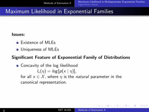
Issues:
Existence of MLEs
Uniqueness of MLEs
Significant Feature of Exponential Family of Distributions
Concavity of the log likelihood lx (η) = log [p(x | η)],
for all x ∈ X , where η is the natural parameter in the canonical representation.
3 MIT 18.655 Methods of Estimation II
Methods of Estimation II Maximum Likelihood in Multiparameter Exponential Families Algorithmic Issues
Existence and Uniqueness Theorem
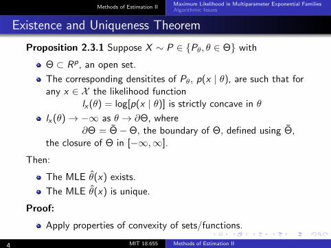
Proposition 2.3.1 Suppose X ∼ P ∈ {Pθ, θ ∈ Θ} with
Θ ⊂ Rp, an open set.
The corresponding densitites of Pθ, p(x | θ), are such that for any x ∈ X the likelihood function
lx (θ) = log[p(x | θ)] is strictly concave in θ
lx (θ) → −∞ as θ → ∂Θ, where ¯ ¯∂Θ = Θ − Θ, the boundary of Θ, defined using Θ,
the closure of Θ in [−∞, ∞].
Then:
The MLE θ̂(x) exists.
The MLE θ̂(x) is unique.
Proof:
Apply properties of convexity of sets/functions.
4 MIT 18.655 Methods of Estimation II
Methods of Estimation II Maximum Likelihood in Multiparameter Exponential Families Algorithmic Issues
Convexity
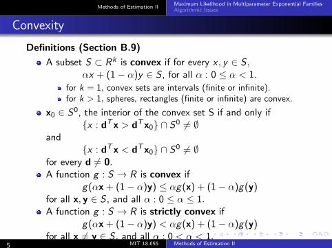
Definitions (Section B.9)
A subset S ⊂ Rk is convex if for every x , y ∈ S , αx + (1 − α)y ∈ S , for all α : 0 ≤ α < 1.
for k = 1, convex sets are intervals (finite or infinite). for k > 1, spheres, rectangles (finite or infinite) are convex.
x0 ∈ S0, the interior of the convex set S if and only if {x : dT x > dT x0} ∩ S0 = ∅
and {x : dT x < dT x0} ∩ S0 = ∅
for every d = 0. A function g : S → R is convex if
g(αx + (1 − α)y) ≤ αg(x) + (1 − α)g(y) for all x, y ∈ S , and all α : 0 ≤ α ≤ 1. A function g : S → R is strictly convex if
g(αx + (1 − α)y) < αg(x) + (1 − α)g(y)
MIT 18.655 Methods of Estimation II for all x = y ∈ S , and all α : 0 < α < 1.
5
Methods of Estimation II Maximum Likelihood in Multiparameter Exponential Families Algorithmic Issues
Convexity
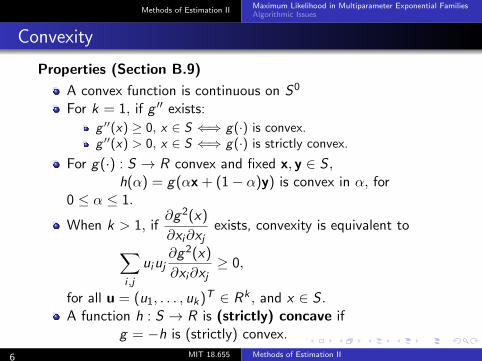
Properties (Section B.9)
A convex function is continuous on S0
For k = 1, if g ii exists: g ll(x) ≥ 0, x ∈ S ⇐⇒ g(·) is convex. g ll(x) > 0, x ∈ S ⇐⇒ g(·) is strictly convex.
For g(·) : S → R convex and fixed x, y ∈ S , h(α) = g(αx + (1 − α)y) is convex in α, for
0 ≤ α ≤ 1. ∂g2(x)
When k > 1, if exists, convexity is equivalent to∂xi ∂xj ∂g2(x)
ui uj ≥ 0, i ,j
∂xi ∂xj
for all u = (u1, . . . , uk )T ∈ Rk , and x ∈ S .
A function h : S → R is (strictly) concave if g = −h is (strictly) convex.
6 MIT 18.655 Methods of Estimation II
Methods of Estimation II Maximum Likelihood in Multiparameter Exponential Families Algorithmic Issues
Convexity
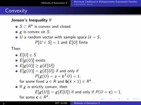
Jensen’s Inequality If
S ⊂ Rk is convex and closed g is convex on S . U a random vector with sample space U = S ,
P[U ∈ S ] = 1 and E [U] finite
Then
E [U] ∈ S E [g(U)] exists E [g(U)] ≥ g(E [U]) E [g(U)] = g(E [U]) if and only if
P(g(U) = a + bT U) = 1. for some fixed a ∈ R and b(k × 1) ∈ Rk . If g is strictly convex, then
E [g(U)] = g(E [U]) if and only if P(U = c) = 1, for some c ∈ Rk .
7 MIT 18.655 Methods of Estimation II
Methods of Estimation II Maximum Likelihood in Multiparameter Exponential Families Algorithmic Issues
Existence and Uniqueness of MLE
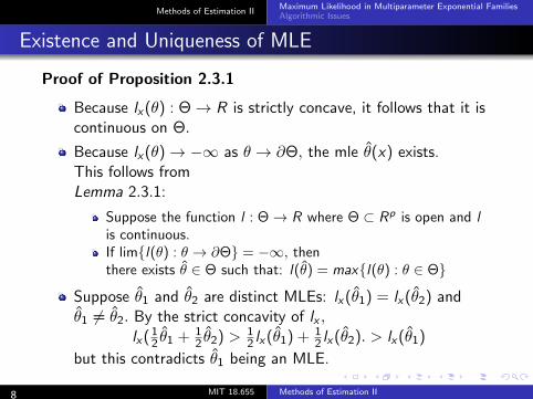
Proof of Proposition 2.3.1
Because lx (θ) : Θ → R is strictly concave, it follows that it is continuous on Θ.
Because lx (θ) → −∞ as θ → ∂Θ, the mle θ̂(x) exists. This follows from Lemma 2.3.1:
Suppose the function l : Θ → R where Θ ⊂ Rp is open and l is continuous. If lim{l(θ) : θ → ∂Θ} = −∞, then there exists θ̂ ∈ Θ such that: l(θ̂) = max{l(θ) : θ ∈ Θ}
Suppose θ̂1 and θ̂2 are distinct MLEs: lx (θ̂1) = lx (θ̂2) and ˆ ˆθ1 = θ2. By the strict concavity of lx ,
(1 ˆ 1 ˆ 1 (ˆ (ˆ (ˆlx θ1 + θ2) > lx θ1) + 1 lx θ2). > lx θ1)2 2 2 2
but this contradicts θ̂1 being an MLE.
8 MIT 18.655 Methods of Estimation II
6=
Methods of Estimation II Maximum Likelihood in Multiparameter Exponential Families Algorithmic Issues
MLEs for Canonical Exponential Family
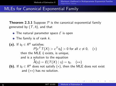
Theorem 2.3.1 Suppose P is the canonical exponential family generated by (T , h), and that
The natural parameter space E is open
The family is of rank k.
(a). If t0 ∈ Rk satisfies: P[cT T (X ) > cT t0] > 0 for all c = 0, (∗)
then the MLE η̂ exists, is unique, and is a solution to the equation
•
A(η) = E (T (X ) | η) = t0. (∗∗) (b). If t0 ∈ Rk does not satisfy (∗), then the MLE does not exist
and (∗∗) has no solution.
9 MIT 18.655 Methods of Estimation II
6=
Methods of Estimation II Maximum Likelihood in Multiparameter Exponential Families Algorithmic Issues
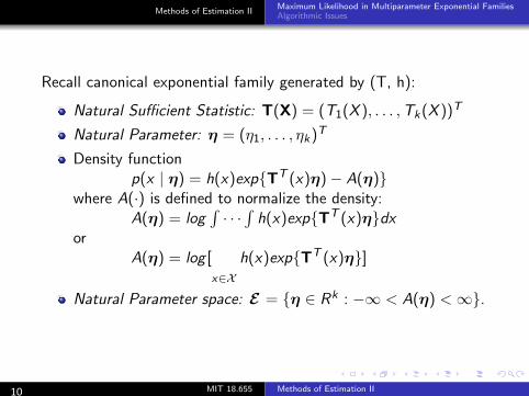
Recall canonical exponential family generated by (T, h):
Natural Sufficient Statistic: T(X) = (T1(X ), . . . , Tk (X ))T
Natural Parameter: η = (η1, . . . , ηk )T
Density function p(x | η) = h(x)exp{TT (x)η) − A(η)}
where A(·) is defined to normalize the density: o o A(η) = log · · · h(x)exp{TT (x)η}dx
or A(η) = log [ h(x)exp{TT (x)η}]
x∈X
Natural Parameter space: E = {η ∈ Rk : −∞ < A(η) < ∞}.
10 MIT 18.655 Methods of Estimation II
Methods of Estimation II Maximum Likelihood in Multiparameter Exponential Families Algorithmic Issues
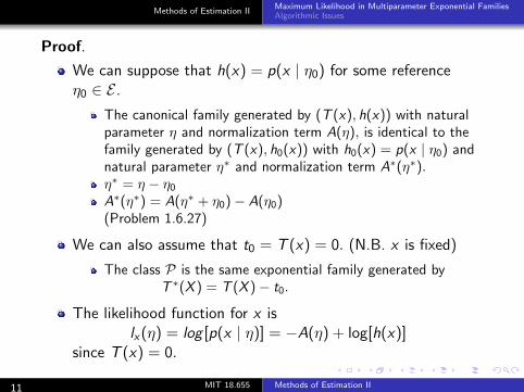
Proof.
We can suppose that h(x) = p(x | η0) for some reference η0 ∈ E .
The canonical family generated by (T (x), h(x)) with natural parameter η and normalization term A(η), is identical to the family generated by (T (x), h0(x)) with h0(x) = p(x | η0) and natural parameter η∗ and normalization term A∗(η∗). η∗ = η − η0
A∗(η∗) = A(η∗ + η0) − A(η0) (Problem 1.6.27)
We can also assume that t0 = T (x) = 0. (N.B. x is fixed)
The class P is the same exponential family generated by T ∗(X ) = T (X ) − t0.
The likelihood function for x is lx (η) = log [p(x | η)] = −A(η) + log[h(x)]
since T (x) = 0.
11 MIT 18.655 Methods of Estimation II
Methods of Estimation II Maximum Likelihood in Multiparameter Exponential Families Algorithmic Issues
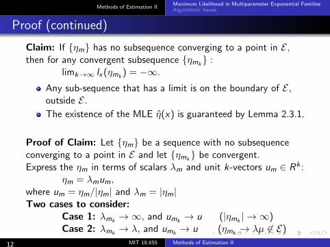
Proof (continued)
Claim: If {ηm} has no subsequence converging to a point in E , then for any convergent subsequence {ηmk } :
limk→∞ lx (ηmk ) = −∞.
Any sub-sequence that has a limit is on the boundary of E , outside E . The existence of the MLE η̂(x) is guaranteed by Lemma 2.3.1.
Proof of Claim: Let {ηm} be a sequence with no subsequence converging to a point in E and let {ηmk } be convergent. Express the ηm in terms of scalars λm and unit k-vectors um ∈ Rk :
ηm = λmum, where um = ηm/|ηm| and λm = |ηm|Two cases to consider:
Case 1: λmk → ∞, and umk → u (|ηmk | → ∞) Case 2: λmk → λ, and umk → u (ηmk → λµ ∈ E)
12 MIT 18.655 Methods of Estimation II
Methods of Estimation II Maximum Likelihood in Multiparameter Exponential Families Algorithmic Issues
Proof (continued)
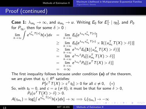
Case 1: λmk → ∞, and umk → u. Writing E0 for E [· | η0], and P0
for Pη0 , then for some δ > 0 : / TηT T (x) λmk
u T (x)mk mklim e h(x)dx = lim E0[e ] k→∞ k→∞
Tλmk umk T (x) T≥ lim E0[e × 1({u T (X ) > δ})]mkk→∞
λmk T≥ lim e δ E0[1({u T (X ) > δ})]mkk→∞ T = lim e λmk δ P0[{u T (X ) > δ}]mkk→∞
= lim e λmk δ P0[{u T T (X ) > δ}] k→∞
= +∞ The first inequality follows because under condition (a) of the theorem, we are given that t0 ∈ Rk satisfies:
P[cT T (X ) > cT t0] > 0 for all c = 0, (∗) So, with t0 = 0, and c = u (= 0), it must be that for some δ > 0,
P0(uT T (X ) > δ) > 0. o ηT
mk T (x)A(ηmk ) = log[ e h(x)dx ] → ∞ =⇒ lx (ηmk ) → −∞
13 MIT 18.655 Methods of Estimation II
6=6=
Methods of Estimation II Maximum Likelihood in Multiparameter Exponential Families Algorithmic Issues
Proof (continued)
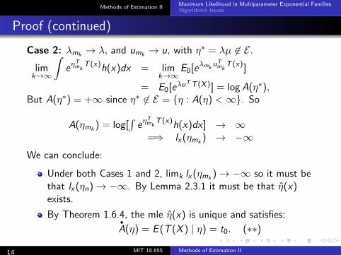
Case 2: λmk → λ, and umk → u, with η∗ = λµ ∈ E ./ TηT T (x) u T (x)mk
λmk mklim e h(x)dx = lim E0[e ] k→∞ k→∞
λu= E0[eTT (X )] = log A(η∗),
But A(η∗) = +∞ since η∗ ∈ E = {η : A(η) < ∞}. So o ηT T (x)A(ηmk ) = log[ e mk h(x)dx ] → ∞ =⇒ lx (ηmk ) → −∞
We can conclude:
Under both Cases 1 and 2, limk lx (ηmk ) → −∞ so it must be that lx (ηn) → −∞. By Lemma 2.3.1 it must be that η̂(x) exists.
By Theorem 1.6.4, the mle η̂(x) is unique and satisfies: •
A(η) = E (T (X ) | η) = t0. (∗∗)
14 MIT 18.655 Methods of Estimation II
Methods of Estimation II Maximum Likelihood in Multiparameter Exponential Families Algorithmic Issues
Proof (continued)
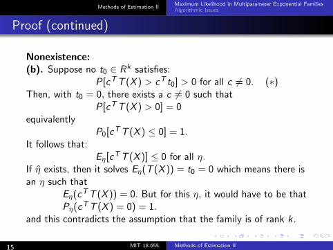
Nonexistence: (b). Suppose no t0 ∈ Rk satisfies:
P[cT T (X ) > cT t0] > 0 for all c = 0. (∗) Then, with t0 = 0, there exists a c = 0 such that
P[cT T (X ) > 0] = 0 equivalently
P0[cT T (X ) ≤ 0] = 1.
It follows that: Eη[c
T T (X )] ≤ 0 for all η. If η̂ exists, then it solves Eη(T (X )) = t0 = 0 which means there is an η such that
Eη(cT T (X )) = 0. But for this η, it would have to be that
Pη(cT T (X ) = 0) = 1.
and this contradicts the assumption that the family is of rank k.
15 MIT 18.655 Methods of Estimation II
6=6=
Methods of Estimation II Maximum Likelihood in Multiparameter Exponential Families Algorithmic Issues
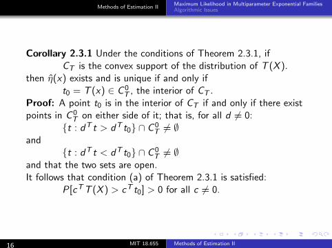
Corollary 2.3.1 Under the conditions of Theorem 2.3.1, if CT is the convex support of the distribution of T (X ).
then η̂(x) exists and is unique if and only if t0 = T (x) ∈ C 0 , the interior of CT .T
Proof: A point t0 is in the interior of CT if and only if there exist points in C 0 on either side of it; that is, for all d = 0: T
{t : dT t > dT t0} ∩ C 0 = ∅T and
{t : dT t < dT t0} ∩ C 0 = ∅T and that the two sets are open. It follows that condition (a) of Theorem 2.3.1 is satisfied:
P[cT T (X ) > cT t0] > 0 for all c = 0.
16 MIT 18.655 Methods of Estimation II
6=6=
6=
6=
Methods of Estimation II Maximum Likelihood in Multiparameter Exponential Families Algorithmic Issues
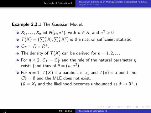
Example 2.3.1 The Gaussian Model.
X1, . . . , Xn iid N(µ, σ2), with µ ∈ R, and σ2 > 0 X 2 iT (X ) = ( n Xi ,
n ) is the natural sufficieint statistic. 1 1
CT = R × R+ .
The density of T (X ) can be derived for n = 1, 2, . . .
= C 0
exists (and thus of θ = (µ, σ2).
For n = 1, T (X ) is a parabola in x1 and T (x) is a point. So
TFor n ≥ 2, CT and the mle of the natural parameter η
C 0 = ∅ and the MLE does not exist. (µ̂ = X1 and the likelihood becomes unbounded as σ̂ → 0+ T
.)
17 MIT 18.655 Methods of Estimation II
Methods of Estimation II Maximum Likelihood in Multiparameter Exponential Families Algorithmic Issues
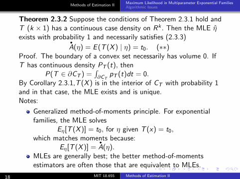
Theorem 2.3.2 Suppose the conditions of Theorem 2.3.1 hold and T (k × 1) has a continuous case density on Rk . Then the MLE η̂ exists with probability 1 and necessarily satisfies (2.3.3)
•
A(η) = E (T (X ) | η) = t0. (∗∗) Proof. The boundary of a convex set necessarily has volume 0. If T has continuous density PT (t), then o
P(T ∈ ∂CT ) = ∂CT pT (t)dt = 0.
By Corollary 2.3.1,T (X ) is in the interior of CT with probability 1 and in that case, the MLE exists and is unique. Notes:
Generalized method-of-moments principle. For exponential families, the MLE solves
Eη[T (X )] = t0, for η given T (x) = t0, which matches moments because:
•
A(η).Eη[T (X )] = MLEs are generally best; the better method-of-moments estimators are often those that are equivalent to MLEs.
18 MIT 18.655 Methods of Estimation II
Methods of Estimation II Maximum Likelihood in Multiparameter Exponential Families Algorithmic Issues
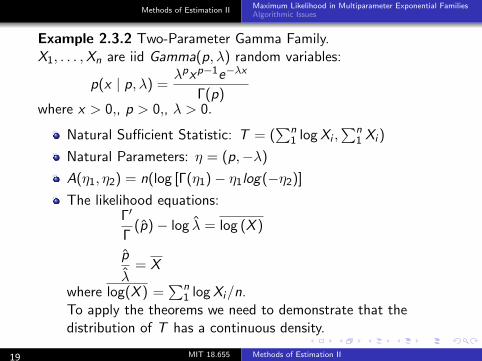
Example 2.3.2 Two-Parameter Gamma Family. X1, . . . , Xn are iid Gamma(p, λ) random variables:
λp p−1 −λxx ep(x | p, λ) =
Γ(p) where x > 0,, p > 0,, λ > 0.
Natural Sufficient Statistic: T = ( n 1 log Xi ,
n 1 Xi )
Natural Parameters: η = (p, −λ)
A(η1, η2) = n(log [Γ(η1) − η1log(−η2)]
The likelihood equations: Γi
Γ (p̂) − log λ̂ = log (X )
p̂
λ̂ = X
where log(X ) = n 1 log Xi /n.
To apply the theorems we need to demonstrate that the distribution of T has a continuous density.
19 MIT 18.655 Methods of Estimation II
∑ ∑
∑
••
••
�
Methods of Estimation II Maximum Likelihood in Multiparameter Exponential Families Algorithmic Issues
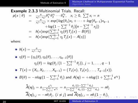
Example 2.3.3 Multinomial Trials. Recall: n θx1 θx2 xq qp(x | θ) = · · · θq , xi ≥ 0, 1 xi = n x1!···xq ! 1 2 n = × exp{log(θ1)x1 + · · · + log(θq−1)xq−1x1!···xq !
q−1 q−1 +log(1 − θj )[n − xj ]}1 1 q−1 = h(x)exp{ ηj (θ)Tj (x) − B(θ)}j=1 q−1 = h(x)exp{ ηj Tj (x) − A(η)}j=1
where:
nh(x) = x1!···xq !
η(θ) = (η1(θ), η2(θ), . . . , ηq−1(θ))
ηj (θ) = log(θj /(1 − q−1 θj )), j = 1, . . . , q − 11
T (x) = (X1, X2, . . . , Xq−1) = (T1(x), T2(x), . . . , Tq−1(x)).
q−1 q−1B(θ) = −nlog(1 − θj ) and A(η) = +nlog(1 + eηj )j=1 j=1
• q−1 e ηj θj /(1− θk )A(η)j = n � ηj
= n � 1 � = nθjq−1 q−1 q−11+ e 1+ θk /(1− θk )j=1 1 1
A(η)i,j = −nθi θj , (i = j) and A(η)i,i = nθi (1 − θi ),
20 MIT 18.655 Methods of Estimation II
∑∑ ∑∑∑
∑∑ ∑
6=
Methods of Estimation II Maximum Likelihood in Multiparameter Exponential Families Algorithmic Issues
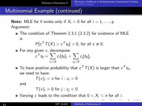
Multinomial Example (continued)
Note: MLE for θ exists only if Xi > 0 for all i = 1, . . . , q Argument:
The condition of Theorem 2.3.1 (2.3.2) for existence of MLE is
P[cT T (X ) > cT t0] > 0, for all c = 0.
For any given c , decompose: cT t0 = ci [t0]i + cj [t0]j
ci >0 cj <0
To have positive probability that cT T (X ) is larger than cT t0, we need to have:
T (x)i < n for i : ci > 0 and
T (x)i > 0 for j : cj < 0
Varying c leads to the condition that 0 < Xi < n for all i .
21 MIT 18.655 Methods of Estimation II
∑ ∑6=
Methods of Estimation II Maximum Likelihood in Multiparameter Exponential Families Algorithmic Issues
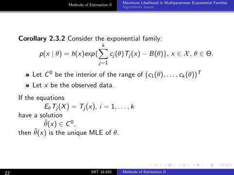
Corollary 2.3.2 Consider the exponential family: k
p(x | θ) = h(x)exp{ cj (θ)Tj (x) − B(θ)}, x ∈ X , θ ∈ Θ. j=1
Let C 0 be the interior of the range of (c1(θ), . . . , ck (θ))T
Let x be the observed data.
If the equations EθTj (X ) = Tj (x), i = 1, . . . , k
have a solution θ̂(x) ∈ C 0 ,
then θ̂(x) is the unique MLE of θ.
22 MIT 18.655 Methods of Estimation II
∑
Methods of Estimation II Maximum Likelihood in Multiparameter Exponential Families Algorithmic Issues
Outline
1 Methods of Estimation II Maximum Likelihood in Multiparameter Exponential Families Algorithmic Issues
23 MIT 18.655 Methods of Estimation II
Methods of Estimation II Maximum Likelihood in Multiparameter Exponential Families Algorithmic Issues
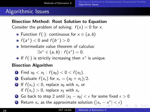
Algorithmic Issues
Bisection Method: Root Solution to Equation Consider the problem of solving: f (x) = 0 for x .
Function f (·): continuous for x ∈ (a, b) f (a+) < 0 and f (b−) > 0 Intermediate value theorem of calculus:
∗∃x ∈ (a, b) : f (x ∗) = 0. ∗If f (·) is strictly increasing then x is unique.
Bisection Algorithm
1
2
Find x0 < x1 : f (x0) < 0 < f (x1). Evaluate f (x∗) for x∗ = (x0 + x1)/2.
3 If f (x∗) < 0, replace x0 with x∗ or if f (x∗) > 0, replace x1 with x∗
4 Go back to step 2 until |x1 − x0| < E for some fixed E > 0 5 Return x∗ as the approximate solution (|x∗ − x ∗| < E)
24 MIT 18.655 Methods of Estimation II
Methods of Estimation II Maximum Likelihood in Multiparameter Exponential Families Algorithmic Issues
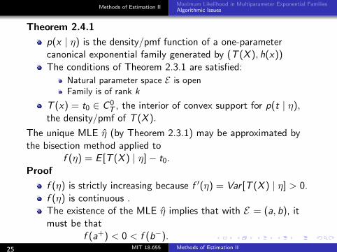
Theorem 2.4.1
p(x | η) is the density/pmf function of a one-parameter canonical exponential family generated by (T (X ), h(x)) The conditions of Theorem 2.3.1 are satisfied:
Natural parameter space E is open Family is of rank k
T (x) = t0 ∈ C 0 , the interior of convex support for p(t | η),T the density/pmf of T (X ).
The unique MLE η̂ (by Theorem 2.3.1) may be approximated by the bisection method applied to
f (η) = E [T (X ) | η] − t0. Proof
f (η) is strictly increasing because f i(η) = Var [T (X ) | η] > 0. f (η) is continuous . The existence of the MLE η̂ implies that with E = (a, b), it must be that
f (a+) < 0 < f (b−). 25 MIT 18.655 Methods of Estimation II
Methods of Estimation II Maximum Likelihood in Multiparameter Exponential Families Algorithmic Issues
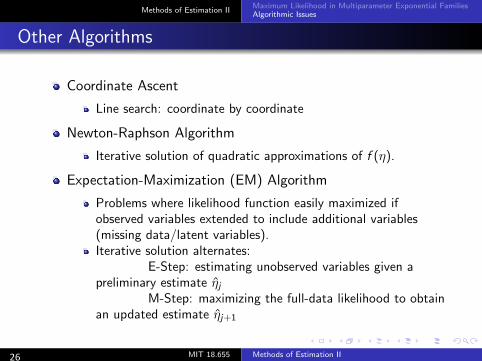
Other Algorithms
Coordinate Ascent
Line search: coordinate by coordinate
Newton-Raphson Algorithm
Iterative solution of quadratic approximations of f (η).
Expectation-Maximization (EM) Algorithm
Problems where likelihood function easily maximized if observed variables extended to include additional variables (missing data/latent variables). Iterative solution alternates:
E-Step: estimating unobserved variables given a preliminary estimate η̂j
M-Step: maximizing the full-data likelihood to obtain an updated estimate η̂j+1
26 MIT 18.655 Methods of Estimation II
Methods of Estimation II Maximum Likelihood in Multiparameter Exponential Families Algorithmic Issues
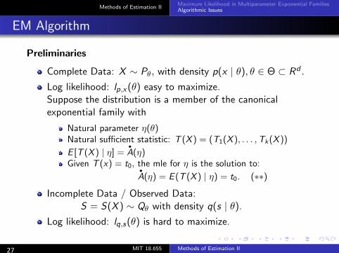
EM Algorithm
Preliminaries
Complete Data: X ∼ Pθ, with density p(x | θ), θ ∈ Θ ⊂ Rd .
Log likelihood: lp,x (θ) easy to maximize. Suppose the distribution is a member of the canonical exponential family with
Natural parameter η(θ) Natural sufficient statistic: T (X ) = (T1(X ), . . . , Tk (X ))
•
E [T (X ) | η] = A(η) Given T (x) = t0, the mle for η is the solution to:
•
A(η) = E (T (X ) | η) = t0. (∗∗)
Incomplete Data / Observed Data: S = S(X ) ∼ Qθ with density q(s | θ).
Log likelihood: lq,s (θ) is hard to maximize.
27 MIT 18.655 Methods of Estimation II
Methods of Estimation II Maximum Likelihood in Multiparameter Exponential Families Algorithmic Issues
EM Algorithm
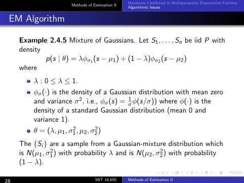
Example 2.4.5 Mixture of Gaussians. Let S1, . . . , Sn be iid P with density
p(s | θ) = λφσ1 (s − µ1) + (1 − λ)φσ2 (s − µ2) where
λ : 0 ≤ λ ≤ 1.
φσ(·) is the density of a Gaussian distribution with mean zero and variance σ2 , i.e., φσ(s) = 1 φ(s/σ)) where φ(·) is the σ density of a standard Gaussian distribution (mean 0 and variance 1).
θ = (λ, µ1, σ12, µ2, σ2
2)
The {Si } are a sample from a Gaussian-mixture distribution which is N(µ1, σ1
2) with probability λ and is N(µ2, σ22) with probability
(1 − λ).
28 MIT 18.655 Methods of Estimation II
Methods of Estimation II Maximum Likelihood in Multiparameter Exponential Families Algorithmic Issues
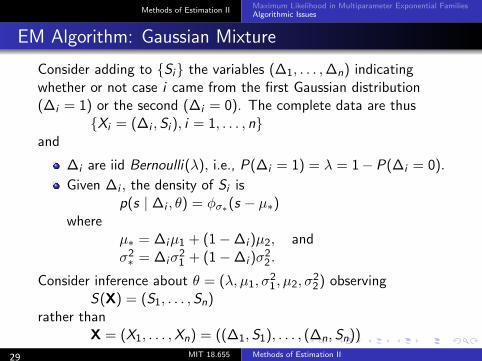
EM Algorithm: Gaussian Mixture
Consider adding to {Si } the variables (Δ1, . . . , Δn) indicating whether or not case i came from the first Gaussian distribution (Δi = 1) or the second (Δi = 0). The complete data are thus
{Xi = (Δi , Si ), i = 1, . . . , n}and
Δi are iid Bernoulli(λ), i.e., P(Δi = 1) = λ = 1 − P(Δi = 0). Given Δi , the density of Si is
p(s | Δi , θ) = φσ∗ (s − µ∗) where
µ∗ = Δi µ1 + (1 − Δi )µ2, and σ∗ 2 = Δi σ1
2 + (1 − Δi )σ22 .
Consider inference about θ = (λ, µ1, σ12, µ2, σ2
2) observing S(X) = (S1, . . . , Sn)
rather than X = (X1, . . . , Xn) = ((Δ1, S1), . . . , (Δn, Sn))
29 MIT 18.655 Methods of Estimation II
Methods of Estimation II Maximum Likelihood in Multiparameter Exponential Families Algorithmic Issues
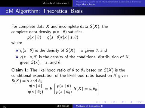
EM Algorithm: Theoretical Basis
For complete data X and incomplete data S(X ), the complete-data density p(x | θ) satisfies
p(x | θ) = q(s | θ)r(x | s, θ) where
q(s | θ) is the density of S(X ) = s given θ, and
r(x | s, θ) is the density of the conditional distribution of X given S(x) = s, and θ.
Claim 1: The likelihood ratio of θ to θ0 based on S(X ) is the conditional expectation of the likelihood ratio based on X given S(X ) = s and θ0.
q(s | θ) p(x | θ) = E |S(X ) = s, θ0
q(s | θ0) p(x | θ0)
30 MIT 18.655 Methods of Estimation II
Methods of Estimation II Maximum Likelihood in Multiparameter Exponential Families Algorithmic Issues
EM Algorithm: Theoretical Basis
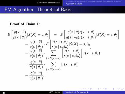
Proof of Claim 1:
p(x | θ) q(s | θ)r(x | s, θ)E |S(X ) = s, θ0 = E |S(X ) = s, θ0
p(x | θ0) q(s | θ0)r(x | s, θ0)q(s | θ) r(x | s, θ)
= · E |S(X ) = s, θ0 q(s | θ0) r(x | s, θ0)q(s | θ) r(x | s, θ)
= · r(x | s, θ0) q(s | θ0) r(x | s, θ0){x :S(x)=s}q(s | θ)
= · [r(x | s, θ)] q(s | θ0) {x :S(x)=s}q(s | θ)
= . q(s | θ0)
31 MIT 18.655 Methods of Estimation II
[ ] [ ][ ]∑ [ ]∑
Methods of Estimation II Maximum Likelihood in Multiparameter Exponential Families Algorithmic Issues
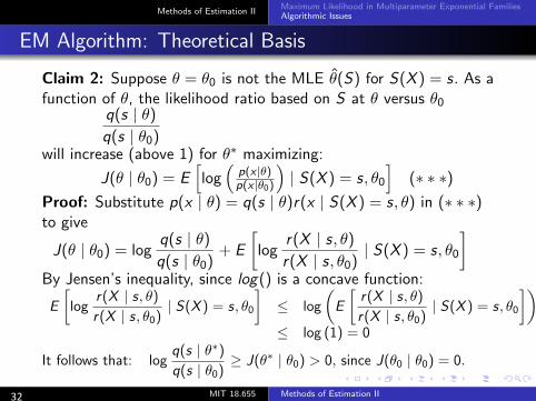
EM Algorithm: Theoretical Basis
Claim 2: Suppose θ = θ0 is not the MLE θ̂(S) for S(X ) = s. As a function of θ, the likelihood ratio based on S at θ versus θ0
q(s | θ) q(s | θ0)
will increase (above 1) for θ∗ maximizing: e m p(x |θ)J(θ | θ0) = E log | S(X ) = s, θ0 (∗ ∗ ∗)p(x |θ0)
Proof: Substitute p(x | θ) = q(s | θ)r(x | S(X ) = s, θ) in (∗ ∗ ∗) to give
q(s | θ) r(X | s, θ)J(θ | θ0) = log + E log | S(X ) = s, θ0
q(s | θ0) r(X | s, θ0) By Jensen’s inequality, since log() is a concave function: n
r(X | s, θ) r(X | s, θ)E log | S(X ) = s, θ0 ≤ log E | S(X ) = s, θ0
r(X | s, θ0) r(X | s, θ0) ≤ log (1) = 0
q(s | θ∗)It follows that: log ≥ J(θ ∗ | θ0) > 0, since J(θ0 | θ0) = 0.
q(s | θ0)
32 MIT 18.655 Methods of Estimation II
[ ][ ] [ ])
Methods of Estimation II Maximum Likelihood in Multiparameter Exponential Families Algorithmic Issues
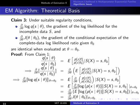
EM Algorithm: Theoretical Basis
Claim 3: Under suitable regularity conditions, ∂ log q(s | θ), the gradient of the log likelihood for the ∂θ incomplete data S , and ∂ J(θ | θ0), the gradient of the conditional expectation of the ∂θ complete-data log likelihood ratio given θ0
are identical when evaluated at θ = θ0. Proof: From Claim 1:
q(s | θ) p(x |θ)= E |S(X ) = s, θ0 q(s | θ0) p(x |θ0) e m q(s | θ) p(x |θ)∂ ∂ =⇒ ∂θ [ q(s | θ0)
] = ∂θ E p(x |θ0) |S(X ) = s, θ0e m ∂ ∂ p(x |θ)=⇒ ∂θ [log q(s | θ)]|θ=θ0 = E ∂θ p(x |θ0) |S(X ) = s, θ0[
∂ = E [log (p(x | θ))]|S(X ) = s, θ0 |θ=θ0∂θ ∂ = (E [log (p(x | θ))]|S(X ) = s, θ0]) |θ=θ0∂θ ∂
MIT 18.655 Methods of Estimation II
= J(θ | θ0)|θ=θ0∂θ
33
][ ][
[
Methods of Estimation II Maximum Likelihood in Multiparameter Exponential Families Algorithmic Issues
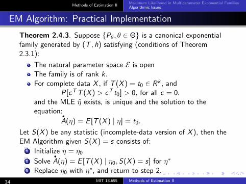
EM Algorithm: Practical Implementation
Theorem 2.4.3. Suppose {Pθ, θ ∈ Θ} is a canonical exponential family generated by (T , h) satisfying (conditions of Theorem 2.3.1):
The natural parameter space E is open The family is of rank k. For complete data X , if T (X ) = t0 ∈ Rk , and
P[cT T (X ) > cT t0] > 0, for all c = 0. and the MLE η̂ exists, is unique and the solution to the equation:
•
A(η) = E [T (X ) | η] = t0.
Let S(X ) be any statistic (incomplete-data version of X ), then the EM Algorithm given S(X ) = s consists of:
1 Initialize η = η0
2 Solve A•
(η) = E [T (X ) | η0, S(X ) = s] for η∗
3 Replace η0 with η∗, and return to step 2.
34 MIT 18.655 Methods of Estimation II
Methods of Estimation II Maximum Likelihood in Multiparameter Exponential Families Algorithmic Issues
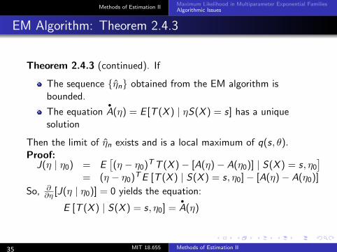
EM Algorithm: Theorem 2.4.3
Theorem 2.4.3 (continued). If
The sequence {η̂n} obtained from the EM algorithm is bounded.
•
The equation A(η) = E [T (X ) | ηS(X ) = s] has a unique solution
Then the limit of η̂n exists and is a local maximum of q(s, θ). Proof: [
J(η | η0) = E (η − η0)T T (X ) − [A(η) − A(η0)] | S(X ) = s, η0
= (η − η0)T E [T (X ) | S(X ) = s, η0] − [A(η) − A(η0)] ∂So, [J(η | η0)] = 0 yields the equation: ∂η
•
E [T (X ) | S(X ) = s, η0] = A(η)
35 MIT 18.655 Methods of Estimation II
]
Methods of Estimation II Maximum Likelihood in Multiparameter Exponential Families Algorithmic Issues
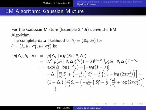
EM Algorithm: Gaussian Mixture
For the Gaussian Mixture (Example 2.4.5) derive the EM Algorithm. The complete-data likelihood of Xi = (Δi , Si ) for θ = (λ, µ1, σ1
2, µ2, σ22) is:
p(Δi , Si | θ) = p(Δi | θ)p(Si | θ, Δi ) = λΔi p(Si | θ, Δi )
Δi (1 − λ)(1−Δi )p(Si | θ, Δi )(1−Δi )
λ = exp{Δi log ( ) − [−log(1 − λ)]1−λe m e m µ1 1 S2 − 1 µ1+Δi Si + −
2
+ log (2πσ2) + σ2 2σ2 i 2 σ2 1 1 e1 m 1 e m
µ(1 − Δi )
µ2 Si + − 1 S2 − 1 22
+ log (2πσ2 σ2 2σ2 i 2 σ2 2) 2 2 2
}
36 MIT 18.655 Methods of Estimation II
[ [
Methods of Estimation II Maximum Likelihood in Multiparameter Exponential Families Algorithmic Issues
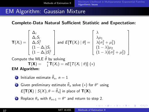
EM Algorithm: Gaussian Mixture
Complete-Data Natural Sufficient Statistic and Expectation: ⎤⎡⎤⎡ Δi λ
T(Xi ) =
⎢⎢⎢⎢⎣
Δi Si Δi S
2 i
(1 − Δi )Si
⎥⎥⎥⎥⎦ and E [T(Xi ) | θ] =
⎢⎢⎢⎢⎣
λµ1 2λ(σ1
2 + µ1) (1 − λ)µ2
⎥⎥⎥⎥⎦ 2(1 − Δi )S
2 (1 − λ)(σ22 + µ2)i
Compute the MLE θ̂ by solving nT(X) = T(Xi ) = nE [T (Xi | θ)] (∗)1
EM Algorithm:
1
2
3
Initialize estimate θ̃n, n = 1
Given preliminary estimate θ̃n solve (∗) for θ∗ using ˜E [T(X) | S(X ), θ = θn] in place of T(X).
Replace θn with θn+1 = θ∗ and return to step 2.
37 MIT 18.655 Methods of Estimation II
Methods of Estimation II Maximum Likelihood in Multiparameter Exponential Families Algorithmic Issues
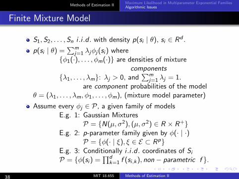
Finite Mixture Model
S1, S2, . . . , Sn i .i .d . with density p(si | θ), si ∈ Rd . m p(si | θ) = λj φj (si ) where j=1
{φ1(·), . . . , φm(·)} are densities of mixture components
m{λ1, . . . , λm}: λj > 0, and λj = 1.j=1 are component probabilities of the model
θ = (λ1, . . . , λm, φ1, . . . , φm), (mixture model parameter)
Assume every φj ∈ P, a given family of models E.g. 1: Gaussian Mixtures
P = {N(µ, σ2), (µ, σ2) ∈ R × R+}E.g. 2: p-parameter family given by φ(· | ·)
P = {φ(· | ξ), ξ ∈ E ⊂ Rp}E.g. 3: Conditionally i .i .d . coordinates of SiodP = {φ(si ) = f (si ,k ), non − parametric f }.k=1
38 MIT 18.655 Methods of Estimation II
∑∑
Methods of Estimation II Maximum Likelihood in Multiparameter Exponential Families Algorithmic Issues
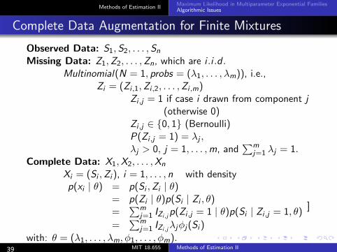
Complete Data Augmentation for Finite Mixtures
Observed Data: S1, S2, . . . , Sn
Missing Data: Z1, Z2, . . . , Zn, which are i .i .d . Multinomial(N = 1, probs = (λ1, . . . , λm)), i.e.,
Zi = (Zi ,1, Zi ,2, . . . , Zi ,m) Zi ,j = 1 if case i drawn from component j
(otherwise 0) Zi ,j ∈ {0, 1} (Bernoulli) P(Zi ,j = 1) = λj ,
mλj > 0, j = 1, . . . , m, and λj = 1.j=1 Complete Data: X1, X2, . . . , Xn
Xi = (Si , Zi ), i = 1, . . . , n with density p(xi | θ) = p(Si , Zi | θ)
= p(Zi | θ)p(Si | Zi , θ) m ]
= j=1 IZi,j p(Zi ,j = 1 | θ)p(Si | Zi ,j = 1, θ) m = IZi,j λj φj (Si )j=1
with: θ = (λ1, . . . , λm, φ1, . . . , φm). 39 MIT 18.655 Methods of Estimation II
∑
∑∑
Methods of Estimation II Maximum Likelihood in Multiparameter Exponential Families Algorithmic Issues
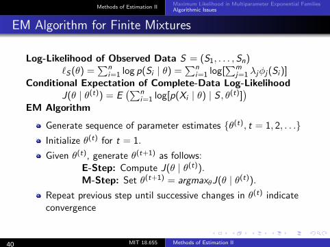
EM Algorithm for Finite Mixtures
Log-Likelihood of Observed Data S = (S1, . . . , Sn) n n mCS (θ) = log p(Si | θ) = log[ λj φj (Si )]i=1 i=1 j=1
Conditional Expectation of Complete-Data Log-Likelihood o -nJ(θ | θ(t)) = E log[p(Xi | θ) | S , θ(t)]i=1 EM Algorithm
Generate sequence of parameter estimates {θ(t), t = 1, 2, . . .}
Initialize θ(t) for t = 1.
Given θ(t), generate θ(t+1) as follows: E-Step: Compute J(θ | θ(t)). M-Step: Set θ(t+1) = argmaxθJ(θ | θ(t)).
Repeat previous step until successive changes in θ(t) indicate convergence
40 MIT 18.655 Methods of Estimation II
∑ ∑ ∑∑
Methods of Estimation II Maximum Likelihood in Multiparameter Exponential Families Algorithmic Issues
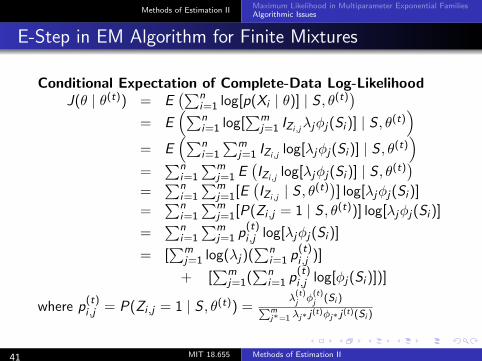
E-Step in EM Algorithm for Finite Mixtures
Conditional Expectation of Complete-Data Log-Likelihood o -nJ(θ | θ(t)) = E log[p(Xi | θ)] | S , θ(t) i=1e m n m = E i=1 log[ j=1 IZi,j λj φj (Si )] | S , θ(t) e m n m = E i=1 j=1 IZi,j log[λj φj (Si )] | S , θ(t) o -n m = i=1 j=1 E IZi,j log[λj φj (Si )] | S , θ(t) o -n m = i=1 j=1[E IZi,j | S , θ(t) ] log[λj φj (Si )]
n m = [P(Zi ,j = 1 | S , θ(t))] log[λj φj (Si )]i=1 j=1n m (t)
= log[λj φj (Si )]i=1 j=1 pi ,j m n (t)
= [ log(λj )( )]j=1 i=1 pi ,j m n (t)
+ [ ( log[φj (Si )])]j=1 i=1 pi ,j (t) (t)
(t) λ φ (Si )where p = P(Zi ,j = 1 | S , θ(t)) = m
j j i ,j λj ∗ j(t)φj ∗ j(t)(Si )j∗=1
41 MIT 18.655 Methods of Estimation II
∑∑ ∑∑ ∑∑ ∑∑ ∑∑ ∑∑ ∑∑ ∑∑ ∑
Methods of Estimation II Maximum Likelihood in Multiparameter Exponential Families Algorithmic Issues
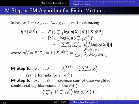
M-Step in EM Algorithm for Finite Mixtures
Solve for θ = (λ1, . . . , λm, φ1, . . . , φm) maximizing o -nJ(θ | θ(t)) = E log[p(Xi | θ)] | S , θ(t) i=1 m n (t)
= [ log(λj )( )]j=1 i=1 pi ,j m n (t)
+ [ ( log[φj (Si )])]j=1 i=1 pi ,j (t) (t)
(t) λj φj (Si )where p = P(Zi ,j = 1 | S , θ(t)) = mi ,j λj∗ j(t)φj∗ j(t)(Si )j ∗ =1
(t+1) 1 n (t)M-Step for λ1, . . . , λm: λ = j n i=1 pi ,j
(t)(same formula for all φ )j
M-Step for φ1, . . . , φm: maximize sum of case-weighted conditional-log-likelihoods of the φj (·)
m n (t)[ ( log[φj (Si )]) ] j=1 i=1 pi ,j
42 MIT 18.655 Methods of Estimation II
∑∑ ∑∑ ∑∑
∑
∑ ∑
Methods of Estimation II Maximum Likelihood in Multiparameter Exponential Families Algorithmic Issues
References
Dempster, AP, Laird, NM, and Rubin, DB (1977). “Maximum Likelihood from Incomplete Data Via the EM Algorithm.” Journal of the Royal Statistial Society. Series B (Methodological), 39(1), 1-38.
Bengalia, T., Chauveau, D. Hunter, D.R., and Young, D.S. “mixtools: An R Package for Analyzing Finite Mixture Models” Journal of Statistial Software, October 2009, Volume 32, Issue 6, 1-29, https://www.jstatsoft.org/article/view/v032i06
43 MIT 18.655 Methods of Estimation II

MIT OpenCourseWarehttp://ocw.mit.edu
18.655 Mathematical StatisticsSpring 2016
For information about citing these materials or our Terms of Use, visit: http://ocw.mit.edu/terms.