U.U.D.M. Project Report 2021:1

Examensarbete i matematik, 15 hpHandledare: Anna SakovichExaminator: Veronica Crispin QuinonezFebruari 2021

Department of MathematicsUppsala University

Mathematical Special Relativity

Ofelia Norgren

Abstract

When Albert Einstein released his theory of special relativity in 1905 itcleared up much of the confusion concerning the properties of light whichappeared to be incompatible with Newtonian Physics. Formulated in thelanguage of kinematics, special relativity postulated that space and time hadto be merged together in a 4-dimensional object, the so-called spacetime, witha clear distinction between space and time. In 1908, Hermann Minkowski,Einstein’s former mathematics professor, presented a geometric interpreta-tion of this merging, a geometry that was subsequently named Minkowskispacetime. The study of this geometry is in fact what special relativity is, inits simplest form.

In this degree project we present the mathematical foundation of specialrelativity, focusing on both classical and modern aspects of the subject. Inparticular, we present a detailed study of the geometry of Minkowski space-time and show how well-known relativistic effects such as the constancy ofthe speed of light and the twin paradox can be explained in terms of thisgeometry. In the final part of this project we discuss a question motivated byproblems in modern cosmology: how to define a valid notion of a distance forMinkowski spacetime which does not carry a positive definite inner product?

Contents

1 Introduction 1

2 Minkowski Spacetime 22.1 The Inner Product . . . . . . . . . . . . . . . . . . . . . . . . 22.2 Pythagoras’s Theorem . . . . . . . . . . . . . . . . . . . . . . 32.3 Basic Causality Theory . . . . . . . . . . . . . . . . . . . . . . 42.4 Basic Theory of Curves in R4

1 . . . . . . . . . . . . . . . . . . 62.5 Lorentz Transformations . . . . . . . . . . . . . . . . . . . . . 7

3 Relativistic Effects 113.1 The Speed of Light . . . . . . . . . . . . . . . . . . . . . . . . 113.2 The Twin Paradox . . . . . . . . . . . . . . . . . . . . . . . . 133.3 Constant Acceleration . . . . . . . . . . . . . . . . . . . . . . 14

4 Minkowski Spacetime as a Metric Space 154.1 Time Functions and Null Distances . . . . . . . . . . . . . . . 164.2 Examples . . . . . . . . . . . . . . . . . . . . . . . . . . . . . 17

5 Conclusion and Discussion 23

References 24

1 Introduction

Light and its properties have long been somewhat of a mystery. The ques-tion to what light actually is gives a very confusing answer, an answer that isboth intricate and easy, in other words a very paradoxical answer. Scientistshad conjectured through history that the elements of light are either wavesor particles but later it was shown that light behaves as both waves and par-ticles at the same time. This wave-particle duality, and, more generally, theuncertainty of the right way to treat light has through history caused somedilemmas and contradictions [1].

In 1887, Albert A. Michelson and Edward Morley conducted an optical ex-periment that would change the view of the properties of light. The classicalMichelson-Morley, or aether-drift, experiment was based on the idea thatthere existed the so-called luminiferous aether, a medium that filled the uni-verse. If light was to be treated as a wave it should travel through thismedium, according to our knowledge of wave motion. In fact, the goal of theMichelson-Morley experiment was to confirm the existence of the luminifer-ous aether, a goal that numerous experiments carried out during the 19thcentury had failed to achieve. The idea of Michelson and Morley was todetect the relative motion of the aether by measuring the speed of light indifferent directions. However, to everyone’s surprise, the experiment showedthat the speed of light was constant in all directions which led to the con-clusion that there was no relative motion between the aether and the earth[1], [2]. This finding was not given any clear explanation back in 1887 andit continued to puzzle physicists for a few years to come. It was not untilEinstein worked out the details of the Michelson-Morley experiment usingthem to create his theory of special relativity that this mystery was clearedup [3].

In fact, all these uncertainties concerning light and its dual properties causedlarge problems for Newtonian Physics, reaching an all time high at the endof the 19th century. As it turned out later, the problem of the Newtonianapproach to light was that it was treated as relative and that its speed wasconsidered to be infinite. In other words, it was thought that there wasno ”speed limit” meaning that the speed of light could (in theory) increaseinfinitely. At the same time, the Michelson-Morley experiment seemed toindicate that the properties of light did not depend on the observer, in par-ticular its speed always appeared to be the same. Albert Einstein was thefirst to realize that the light should be treated as an absolute quantity withthe constant speed c same for all observers. These ideas have subsequently

1

formed the very basis for the theory of special relativity that Einstein pub-lished in 1905 [4], [5].

To express these ideas mathematically Einstein treated space and time quitedifferently from Newtonian mechanics, combining them together into a sin-gle object called spacetime. After the mathematical properties of this objectwere described by Hermann Minkowski in 1908, the spacetime was fittinglynamed Minkowski spacetime [4], [5].

2 Minkowski Spacetime

Roughly speaking, Minkowski spacetime is a geometry needed to explainthe physical universe from the perspective of special relativity. As we willsee in this section, a few characteristics of special relativity that cannot beexplained in terms of Newtonian physics follow rather effortlessly from thegeometry of Minkowski spacetime. We will mostly follow [5] and [6].

2.1 The Inner Product

The coordinate change which Einstein employed to account for the propertiesof light (see Section 2.5 below), arises naturally when 3-dimensional spaceand 1-dimensional time are combined into a certain 4-dimensional object,the so-called Minkowski spacetime denoted by R4

1 [5]. Mathematically, R41

is R4 equipped with the so-called Lorentzian inner product, a symmetricbilinear form η defined as follows. Let e = {e1, e2, e3, e4} be an orthonormalbasis of R4 equipped with the standard Euclidean inner product 〈·, ·〉, andlet v = vaea and w = waea be the coordinate expressions of v, w ∈ R4 in thisbasis. Then

η(v, w) = v1w1 + v2w2 + v3w3 − v4w4. (1)

As we can see, η differs from 〈·, ·〉, which in this case would have the expres-sion

〈v, w〉 = v1w1 + v2w2 + v3w3 + v4w4. (2)

This difference reflects the fact that the direction given by e4 is thought ofas time whereas the linear subspace spanned by {e1, e2, e3} is thought of asspace. Note that the geometric structure of spacetime is coordinated with achoice of an orthonormal basis, e, which in this case is referred to as frameof reference [6].

2

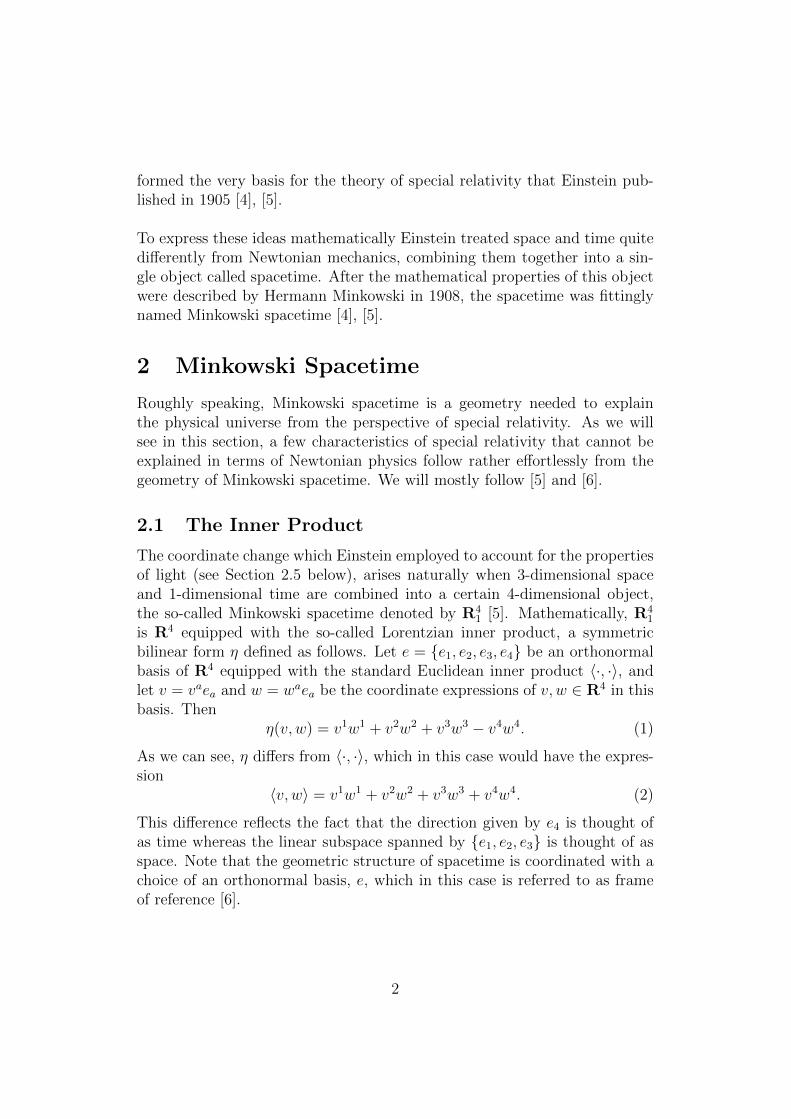
2.2 Pythagoras’s Theorem

As a preliminary to our investigation of the geometry of Minkowski space-time, we take a closer look at the well-known Pythagorean theorem following[7]. One possible formulation of this theorem states that the length of a twodimensional vector with components (dx, dy) is given by

ds2 = dx2 + dy2 (3)

as illustrated in the following picture:

x

y

ds

dx

dy

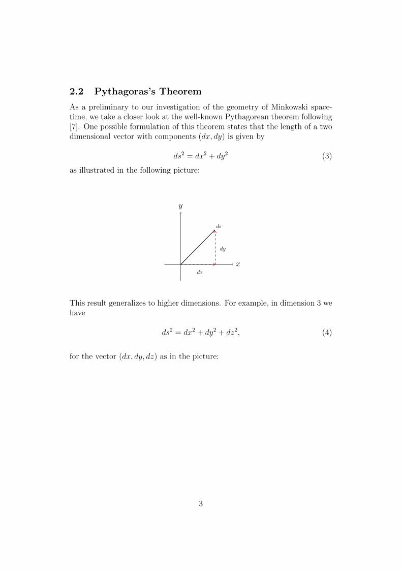
This result generalizes to higher dimensions. For example, in dimension 3 wehave

ds2 = dx2 + dy2 + dz2, (4)

for the vector (dx, dy, dz) as in the picture:

3

z

y

x

ds

dz

dy

dx

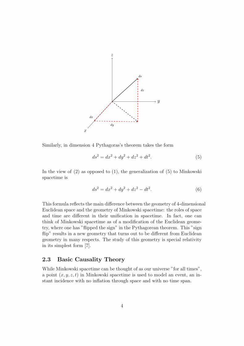
Similarly, in dimension 4 Pythagoras’s theorem takes the form

ds2 = dx2 + dy2 + dz2 + dt2. (5)

In the view of (2) as opposed to (1), the generalization of (5) to Minkowskispacetime is

ds2 = dx2 + dy2 + dz2 − dt2. (6)

This formula reflects the main difference between the geometry of 4-dimensionalEuclidean space and the geometry of Minkowski spacetime: the roles of spaceand time are different in their unification in spacetime. In fact, one canthink of Minkowski spacetime as of a modification of the Euclidean geome-try, where one has ”flipped the sign” in the Pythagorean theorem. This ”signflip” results in a new geometry that turns out to be different from Euclideangeometry in many respects. The study of this geometry is special relativityin its simplest form [7].

2.3 Basic Causality Theory

While Minkowski spacetime can be thought of as our universe ”for all times”,a point (x, y, z, t) in Minkowski spacetime is used to model an event, an in-stant incidence with no inflation through space and with no time span.

4

As explained in Section 2.2, a 4-vector defined by its four components

~ds = (dx, dy, dz, dt) (7)

can be used to measure the interval between two events by means of theformula

ds2 = dx2 + dy2 + dz2 − dt2. (8)

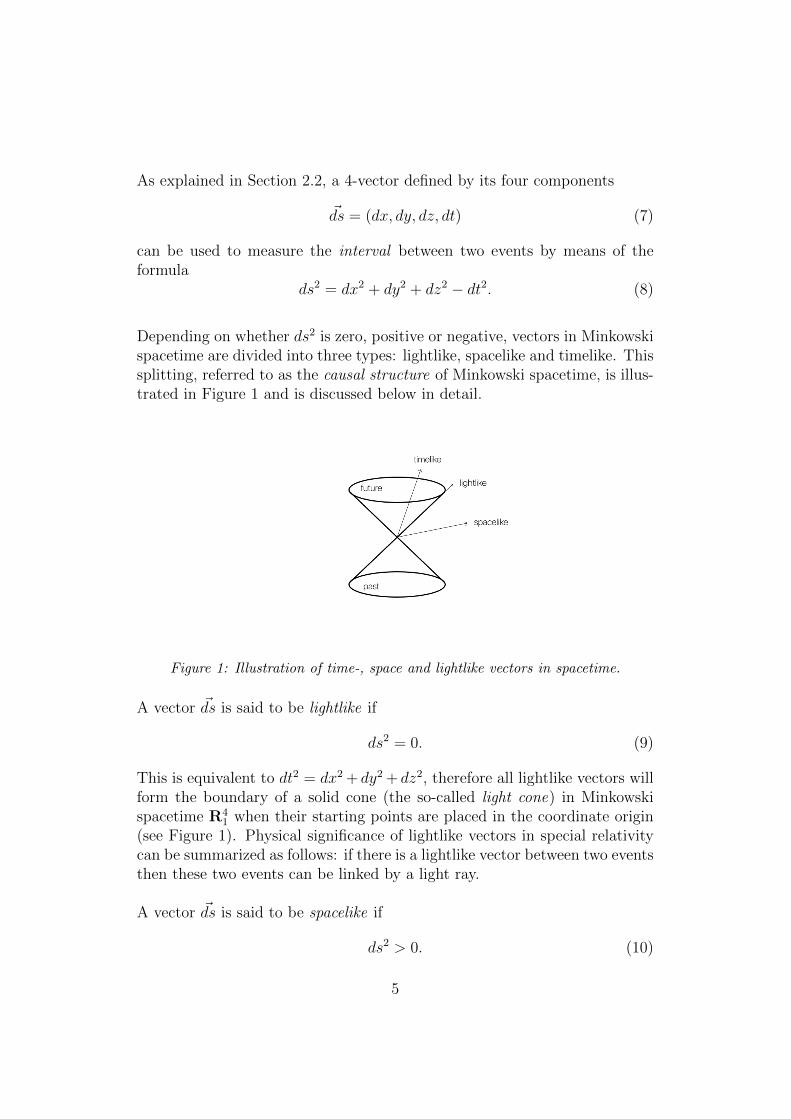
Depending on whether ds2 is zero, positive or negative, vectors in Minkowskispacetime are divided into three types: lightlike, spacelike and timelike. Thissplitting, referred to as the causal structure of Minkowski spacetime, is illus-trated in Figure 1 and is discussed below in detail.

Figure 1: Illustration of time-, space and lightlike vectors in spacetime.

A vector ~ds is said to be lightlike if

ds2 = 0. (9)

This is equivalent to dt2 = dx2 + dy2 + dz2, therefore all lightlike vectors willform the boundary of a solid cone (the so-called light cone) in Minkowskispacetime R4

1 when their starting points are placed in the coordinate origin(see Figure 1). Physical significance of lightlike vectors in special relativitycan be summarized as follows: if there is a lightlike vector between two eventsthen these two events can be linked by a light ray.

A vector ~ds is said to be spacelike if

ds2 > 0. (10)

5

Geometrically, this means that the time component of the vector is smallerthan its space component. As a consequence, all spacelike vectors are locatedoutside of the light cone (see Figure 1). If there is a spacelike vector betweentwo events then there exists a reference frame where these two events happenat the same time but at different locations. This will be explained in detailin Section 2.5.

Finally, a vector ~ds is said to be timelike if

ds2 < 0. (11)

In this case the time component is larger than the space component, whichimplies that all timelike vectors are located inside the light cone (see Figure1). As we will see in Section 2.5, in this case it is possible to find a referenceframe where the respective events happen at the same location but at differ-ent times.

We take yet another look at Figure 1. We may think of a point at thetip of the light cone as the event being observed. Removing the tip, the conesplits into two components, and we may choose one of them to represent thefuture of the event and the other one to represent its past. Such a choicemade consistently for all events is called the time orientation. A timelikevector lying in the future (respectively past) part of the light cone is calledfuture (respectively past) pointing. Note that any event located inside the fu-ture light cone can be caused (or affected) by the event located at the origin.This and some other aspects of causality theory will be further discussed inSection 2.5.

2.4 Basic Theory of Curves in R41

In this section we review some basics concerning curves in R41 that will be

needed for our exploration of relativistic effects in Section 3 and time func-tions and distances in Minkowski spacetime in Section 4.

A curve in R41 is a smooth map

α : I → R s 7→ (x(s), y(s), z(s), t(s)) (12)

where I ⊆ R is a connected nonempty interval. Its velocity vector is com-puted for s ∈ I as

α′(s) = (x′(s), y′(s), z′(s), t′(s)). (13)

6

Just like Euclidean space, Minkowski spacetime can be viewed as a semi-Riemannian manifoldM = (R4

1, γ) whose semi-Riemannian metric γ is givenat all points by the inner product η as described in (1), see e.g. [5]. As aconsequence, the Christoffel symbols of γ vanish, and the (tangential) accel-eration of the curve α is simply

α′′(s) = (x′′(s), y′′(s), z′′(s), t′′(s)). (14)

Recall that α is called a geodesic if it has zero acceleration at all points.In the view of (14) we see that the geodesics of Minkowski spacetime arestraight lines, just like the geodesics of Euclidean space. However, in con-trast to Euclidean case, a straight line between two points in R4

1 is not theshortest of all curves joining the two points. For example, a straight line seg-ment joining (0,−1, 0, 0) and (0, 1, 0, 0) has length 2 whereas a broken linethrough (0,−1, 0, 0), (1, 0, 0, 0) and (0, 1, 0, 0) has length 0, as one readilycomputes using (5). This will become important in Section 4.

Finally, we recall some standard terminology (see e.g. [8]) that will be neededin Section 4. A curve α = α(s) in Minkowski spacetime is called causal if itstangent vector α′(s) given by (13) is either timelike or lightlike for every s. Acausal curve is called future pointing if its tangent vector is future pointingfor all points on the curve.

2.5 Lorentz Transformations

As discussed in Section 2.3, events in special relativity are modelled as pointsof Minkowski spacetime. For describing and localizing events the notionof observer is used, meaning roughly that a choice of a coordinate systemhas been made [6]. If two observers are in relative motion with constantvelocity then the relation between their descriptions of the same event (or,equivalently, the relation between the coordinates of the point representingthe event in the respective coordinate systems) is described by a Lorentztransformation. Lorenz transformations are linear transformations whichpreserve spacetime intervals between points (as defined in Section 2.2). As aconsequence, we may represent a Lorentz transformation by the matrix

Λ =

Λ1

1 Λ12 Λ1

3 Λ14

Λ21 Λ2

2 Λ23 Λ2

4

Λ31 Λ3

2 Λ33 Λ3

4

Λ41 Λ4

2 Λ43 Λ4

4

(15)

which is required to satisfyΛTηΛ = η (16)

7

where ΛT is the transpose of Λ and η is the matrix of the Minkowskian innerproduct given by

η =

1 0 0 00 1 0 00 0 1 00 0 0 −1

(17)

A Lorentz transformation may include a rotation of space, however in spe-cial relativity one is mostly interested in ”space rotation free” Lorentz trans-formation that are called (Lorentz) boosts. Boosts can be thought of asMinkowskian analogues of rotations of Euclidean space where the rotationtakes place in planes spanned by one spacelike and one timelike directionsuch as xt-plane. Boosts and their properties become especially importantwhen it comes to describing well-known relativistic effects, see Section 3.

In order to understand boosts in more detail, we focus on the two dimen-sional case, i.e. we consider the Minkowski plane R2

1 with the coordinates(x, t) and the inner product η given by the matrix

η =

[1 00 −1

](18)

(A detailed treatment of the four dimensional case is very similar in spiritand can be found in [6]).

Theorem 2.1. Let

Λ =

(Λ1

1 Λ12

Λ21 Λ2

2

)(19)

be such that ΛTηΛ = η holds, then Λ is given by

Λ = ±

(1√

1−v2v√1−v2

v√1−v2

1√1−v2

)(20)

for a constant v such that |v| < 1.

Proof. We have

ΛTηΛ =

((Λ1

1)2 − (Λ2

1)2 Λ1

2Λ11 − Λ2

1Λ22

Λ11Λ

12 − Λ2

2Λ21 (Λ1

2)2 − (Λ2

2)2

). (21)

8

As a consequence, the elements of Λ have to satisfy the relations

(Λ1

1)2 − (Λ2

1)2 = 1

Λ12Λ

11 − Λ2

1Λ22 = 0

Λ11Λ

12 − Λ2

2Λ21 = 0

(Λ12)

2 − (Λ22)

2 = −1

(22)

Solving these equations for Λ11, Λ1

2, Λ21 and Λ2

2 we obtainΛ1

1 = ± 1√1−v2

Λ12 = ± v√

1−v2

Λ21 = ± v√

1−v2

Λ22 = ± 1√

1−v2

(23)

for |v| < 11. This gives us Λ as in (20).

The main physical implication of this theorem is the following. Suppose thatwe have an xt-coordinate system associated with a stationary observer andan x′t′-coordinate system associated with an observer that moves in the x-direction with the constant velocity v. If the first observer assigns coordinates(x, t) to an event then in the coordinate system of the second observer theevent will have the coordinates

x′ =1√

1− v2(x− vt)

t′ =1√

1− v2(t− vx)

(24)

The parameter v in this formula is usually referred to as the velocity of theboost.

In the rest of this section we state and prove several important results con-cerning boosts to be used in Section 3.

Theorem 2.2. The inverse transformation to (24) mapping (x′, t′) 7→ (x, t)is the boost of velocity −v, given by the matrix

Λ−1 =

(1√

1−v2v√1−v2

v√1−v2

1√1−v2

)(25)

1One can also express the solutions using hyperbolic functions. In this case Λ lookssimilar to a rotation matrix with sin and cos replaced by sinh and cosh, see [5] for details.

9

Proof. A computation.

As a consequence, we get the following expressions for x and t:{x = 1√

1−v2 (x′ + t′v)

t = 1√1−v2 (t′ + x′v)

(26)

Theorem 2.3. A boost preserves the interval between a point and the origin,i.e. x2−t2 = (x′)2−(t′)2. As a consequence, the causal character is preservedunder a boost, i.e. spacelike vectors are mapped to spacelike vectors, timelikevectors to timelike vectors, and lightlike vectors to lightlike vectors.

Proof. In fact, the statement of the theorem is a consequence of the relationΛTηΛ = η. One can also verify it directly, using (26):

x2 − t2 =1

1− v2(t′v + x′)2 − 1

1− v2(t′ + x′v)2 =

=1

1− v2((t′v + x′)2 − (t′ + x′v)2

)=

=1

1− v2((t′)2v2 + (x′)2 − (t′)2 − (x′)2v2

)=

=1

1− v2(− v2((x′)2 − (t′)2) + ((x′)2 − (t′)2)

)=

=1

1− v2((1− v2)((x′)2 − (t′)2)

)=

= (x′)2 − (t′)2.

(27)

Theorem 2.4. If t > |x| then t′ > |x′| and if t < |x| then t′ < |x|. As aconsequence, a boost preserves the property of a timelike vector to be future(respectively past) pointing.

Proof. We prove the first statement of the theorem, the second one is provensimilarly. Given that t > |x| we have t2 − x2 > 0, whereas by Theorem 2.3we know that x2 − t2 = (x′)2 − (t′)2. This gives

(t′ − |x′|)(t′ + |x′|) > 0. (28)

This inequality implies that either t′ > |x′| or t′ < −|x′|. To see that thesecond option is not possible, it suffices to show that t′ > 0. For this we

10

recall that |v| < 1 hence

vx ≤ |vx| ≤ |v||x| < |x|. (29)

Consequently, we have −vx > −|x| which implies

t′ =t− vx√1− v2

>t− |x|√1− v2

> 0, (30)

and t′ > |x′| follows.

3 Relativistic Effects

Many phenomena in special relativity have natural interpretation in terms ofthe geometry of Minkowski spacetime. In this section we focus on discussingthe constancy of the speed of light, the twin paradox, and the existence of the”speed limit” in special relativity following [5] and [7]. Some other relativisticeffects are explained in [5].

3.1 The Speed of Light

As mentioned in Section 2.5, the causal structure of Minkowski spacetime ispreserved under a boost transformation, in particular, lightlike vectors aremapped to lightlike vectors. We will use this fact to explain why the speedof light is the same for all observers. The example below is adapted from [7].

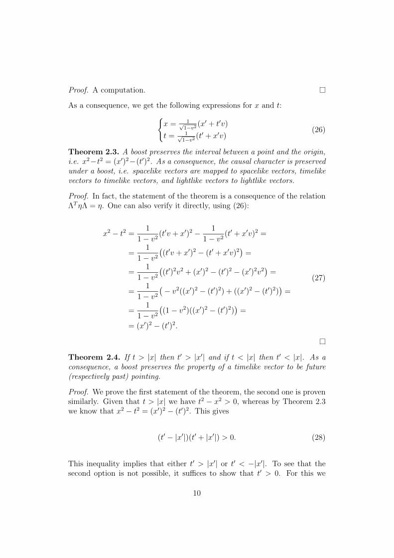
Consider the particles A, B, and C moving in the x-direction as shown inthe picture:

11

t

x

(0,12) A B

(5,13)C (18,18)

To compute the relative velocities of the particles, we will view each of theparticles A and B as an observer by assigning to it a coordinate system inwhich the particle is at x = 0 for all times. As we can see, the chosen coordi-nate system is the one associated with the particle A. From A’s perspective,the particle B is moving with the velocity v = 5

13and the particle C is mov-

ing with the velocity v = 1.

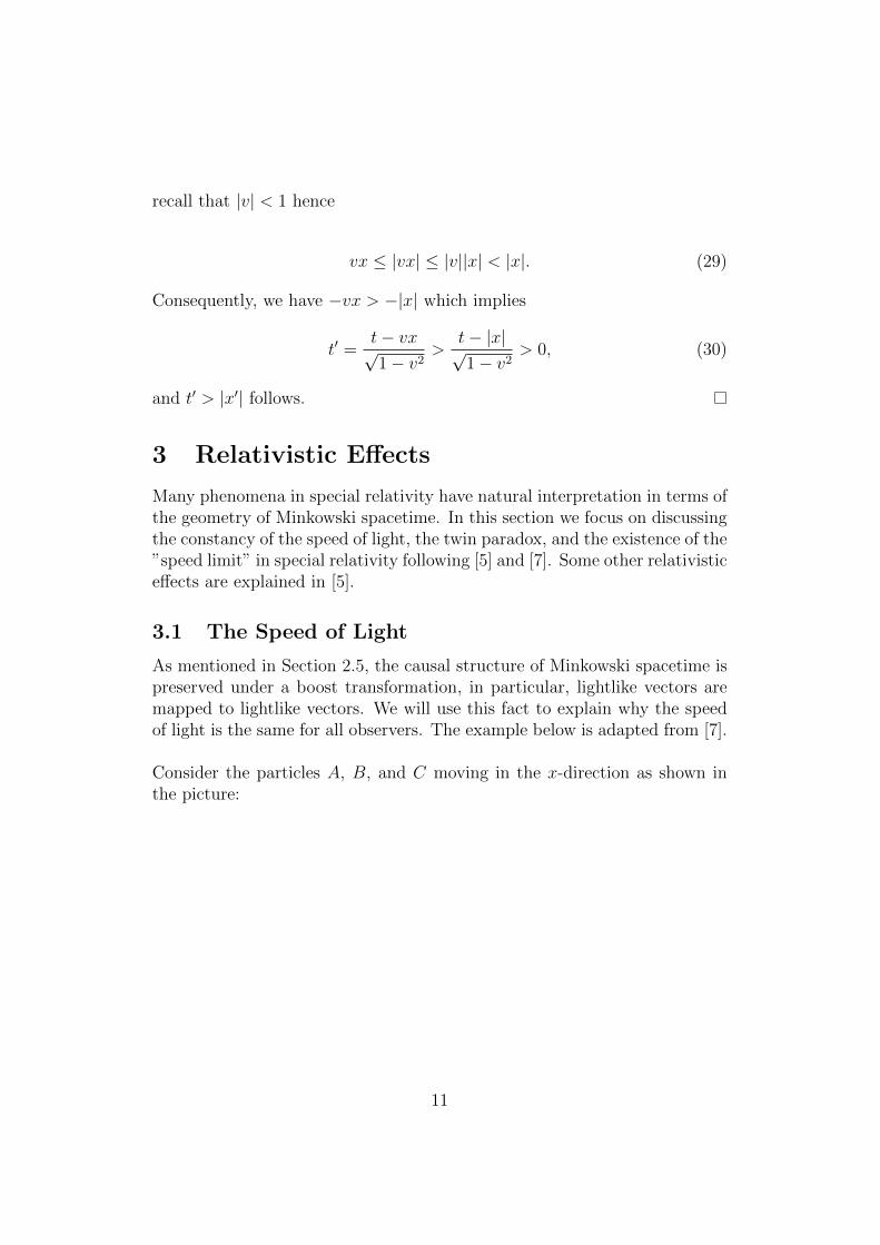
The coordinate system associated with the particle B can be constructed byperforming the boost of velocity v = − 5

13as shown in the picture:

t

x

(0,12) BA

(-5,13)C (18,18)

(12,12)

Here we used the results of Section 2.5 to compute the coordinates of theparticles A and C in this coordinate system. We find that from B’s per-spective A has the velocity v = − 5

13, which is consistent with what was said

earlier about the velocity of B as measured by A. What is more surprising isthat the velocity of C has not changed: measured in the coordinate systemassociated with B it is still 1. This is due to the fact that the vector (18, 18)is lightlike and will remain such after any boost: its components will changebut their ratio will always be 1. As a consequence, the speed of light is c = 1for all observers, not only for A and B.

12

3.2 The Twin Paradox

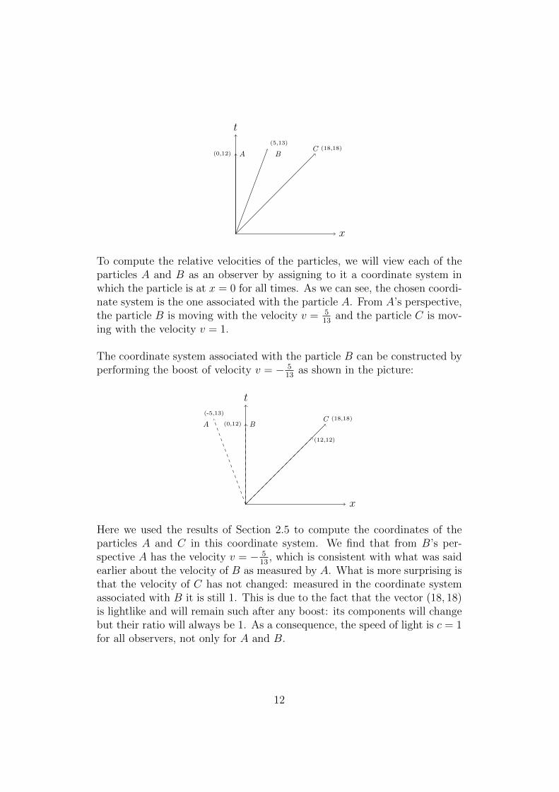
The famous twin paradox is in fact not a paradox but yet another naturalconsequence of the geometry of Minkowski spacetime. Consider two identicaltwins, one of which stays on earth while the other travels 13 years awayfrom earth with the velocity v = 5/13 and then returns back with the samespeed. The time experienced by each twin in his own coordinate system isthe length of his worldline, i.e. the path traversed through spacetime. Thiscan be visualized as follows:

t

x

(0,13)

(0,26)

(5,13) (13,13)

The worldline of the twin staying on earth is the red curve of length 26, sothe time experienced by him is 26 years. The worldline of the second twin isthe dashed blue line. Using Pythagoras’s theorem for Minkowski spacetime(see Section 2.2) we compute that the time experienced by this twin is

2√

132 − 52 = 2√

132 − 52 = 24. (31)

As a consequence, we see that the second twin, who is moving, experiencesless time than the first twin, who is at rest, and should therefore technicallybe younger. Had the second twin moved even faster, with the speed closeto the speed of light, he would have experienced almost no time at all. Tosee this, one computes the length of the black curve representing the lighttravelling 13 years away from earth and then returning back to obtain

2√

132 − 132 = 0. (32)

13

3.3 Constant Acceleration

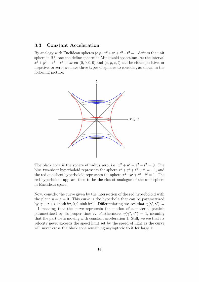
By analogy with Euclidean spheres (e.g. x2 +y2 +z2 + t2 = 1 defines the unitsphere in R4) one can define spheres in Minkowski spacetime. As the intervalx2 + y2 + z2 − t2 between (0, 0, 0, 0) and (x, y, z, t) can be either positive, ornegative, or zero, we have three types of spheres to consider, as shown in thefollowing picture:

t

x, y, z

The black cone is the sphere of radius zero, i.e. x2 + y2 + z2 − t2 = 0. Theblue two-sheet hyperboloid represents the sphere x2 + y2 + z2− t2 = −1, andthe red one-sheet hyperboloid represents the sphere x2+y2+z2−t2 = 1. Thered hyperboloid appears then to be the closest analogue of the unit spherein Euclidean space.

Now, consider the curve given by the intersection of the red hyperboloid withthe plane y = z = 0. This curve is the hyperbola that can be parametrizedby γ : τ 7→ (coshhτ, 0, 0, sinhhτ). Differentiating we see that η(γ′, γ′) =−1 meaning that the curve represents the motion of a material particleparametrized by its proper time τ . Furthermore, η(γ′′, γ′′) = 1, meaningthat the particle is moving with constant acceleration 1. Still, we see that itsvelocity never exceeds the speed limit set by the speed of light as the curvewill never cross the black cone remaining asymptotic to it for large τ .

14

4 Minkowski Spacetime as a Metric Space

We begin this section by recalling the definition of a metric space.

Definition 4.1. [9] Let X be an arbitrary set. A function d : X × X →R ∪ {∞} is a metric on X if the following conditions are satisfied for allx, y, z ∈ X:

(1) d(x, y) > 0 if x 6= y, and d(x, x) = 0.

(2) d(x, y) = d(y, x).

(3) d(x, z) ≤ d(x, y) + d(y, z).

A set X equipped with a metric d is called a metric space.

It is well-known that Euclidean space is a natural metric space whose metricis the distance between two given points as defined by Pythagoras’s theorem.In contrast, Minkowski spacetime does not carry any naturally defined met-ric. In particular, Pythagoras’s theorem cannot be used for defining one as,in particular, the interval between any two points on the light cone is zero,violating (1) in the above definition. See Section 2.2 for more details.

It is important to have a suitable notion of a distance (metric) on Minkowskispacetime as well as on other spacetimes that are important in general rela-tivity and cosmology. This is needed for purposes that require one to comparea given geometry (such as the geometry of our universe) with a model ge-ometry (such as the FLRW model that is used in cosmology to model ouruniverse). In this section we review the basics of the so-called null distanceon Minkowski spacetime as defined by Sormani and Vega in [10]. Whetherthis null distance will ultimately turn out to be a metric or not depends cru-cially on one’s choice of a time function, as will be explained in Section 4.2where two examples from [10] are discussed.

15

4.1 Time Functions and Null Distances

By definition (see e.g. [10]), a generalized time function on n-dimensionalMinkowski spacetime is a function τ : Rn

1 → R that is strictly increasingalong all future-pointing causal curves.

Given a time function, the notion of null distance can be defined as follows.

Definition 4.2. [10] Let τ : Rn1 → R be a generalized time function.

(1) Let β : [a, b] → Rn1 be a piecewise causal curve with breaks a = s0 <

... < sk = b. We set xi = β(si) and define the null length of β by

L̂τ (β) :=k∑i=1

|τ(xi)− τ(xi − 1)|

(2) For any p, q ∈M , we define the null distance by

d̂τ (p, q) := inf {L̂τ (β) : β piecewise causal from p to q}

It turns out that the null distance d̂τ (p, q) satisfies all the axioms of metric(see Definition 4.1) except for possibly the definiteness axiom, i.e. d̂τ (p, q) >0 for p 6= q. Furthermore, when q is in the future of p the null distanced̂τ (p, q) has a very simple expression. This is summarized in the followingresult which was proven (in a more general setting) in [10, Lemma 3.10 andLemma 3.11].

Lemma 4.1. For any generalized time function τ on Rn1 we have

d̂τ (p, q) ≥ |τ(q)− τ(p)| for any p, q ∈ Rn1 .

Consequently, definiteness can only fail for points in the same time slice:

d̂τ (p, q) = 0⇒ τ(q) = τ(p).

Furthermore, if q is in the causal future J+(p) of p (meaning that the vector~pq is either future directed timelike or future directed lightlike) we have

d̂τ (p, q) = τ(q)− τ(p).

16

4.2 Examples

In this section we will investigate which properties make a time function”good” or on contrary ”bad”. A time function τ is considered to be ”good”if the null distance as defined in Definition 4.2 is a metric (see Definition 4.1)and if it encodes the causal structure of spacetime in a certain sense to bemade precise below.

We will now discuss two examples of time functions on Minkowski space-time from [10] and study the properties of the respective null distances indetail.

Example 1

Our first example is concerned with the ”natural” time function τ = t. Inthis case the following has been shown in [10, Proposition 3.3].

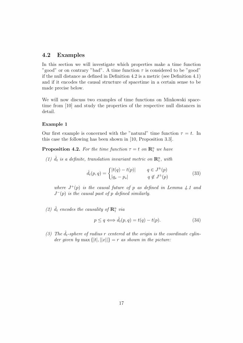
Proposition 4.2. For the time function τ = t on Rn1 we have

(1) d̂t is a definite, translation invariant metric on Rn1 , with

d̂t(p, q) =

{|t(q)− t(p)| q ∈ J±(p)

|qs − ps| q 6∈ J±(p)(33)

where J+(p) is the causal future of p as defined in Lemma 4.1 andJ−(p) is the causal past of p defined similarly.

(2) d̂t encodes the causality of Rn1 via

p ≤ q ⇐⇒ d̂t(p, q) = t(q)− t(p). (34)

(3) The d̂t-sphere of radius r centered at the origin is the coordinate cylin-der given by max {|t|, ||x||} = r as shown in the picture:

17

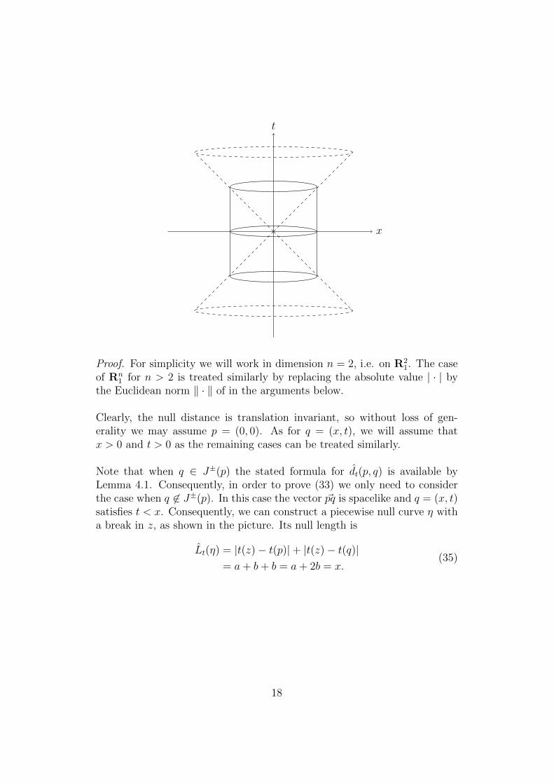
t

x

Proof. For simplicity we will work in dimension n = 2, i.e. on R21. The case

of Rn1 for n > 2 is treated similarly by replacing the absolute value | · | by

the Euclidean norm ‖ · ‖ of in the arguments below.

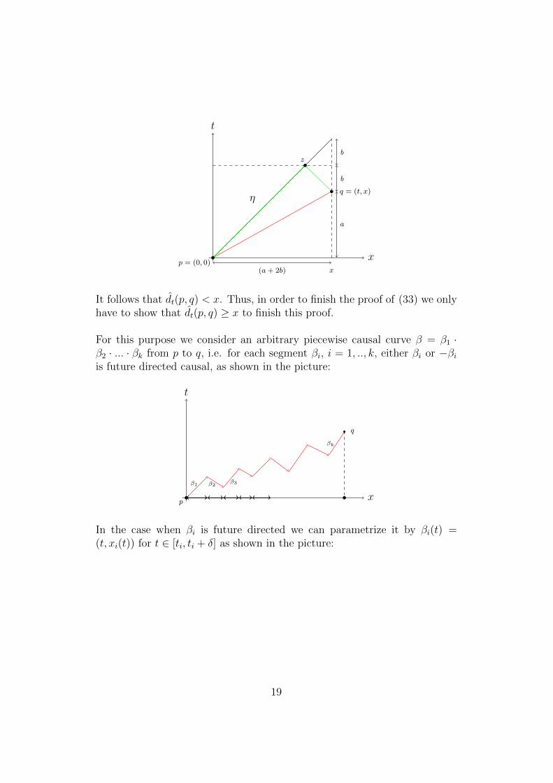
Clearly, the null distance is translation invariant, so without loss of gen-erality we may assume p = (0, 0). As for q = (x, t), we will assume thatx > 0 and t > 0 as the remaining cases can be treated similarly.

Note that when q ∈ J±(p) the stated formula for d̂t(p, q) is available byLemma 4.1. Consequently, in order to prove (33) we only need to considerthe case when q 6∈ J±(p). In this case the vector ~pq is spacelike and q = (x, t)satisfies t < x. Consequently, we can construct a piecewise null curve η witha break in z, as shown in the picture. Its null length is

L̂t(η) = |t(z)− t(p)|+ |t(z)− t(q)|= a+ b+ b = a+ 2b = x.

(35)

18

t

x

η

p = (0, 0)

q = (t, x)

x

z

b

b

a

(a+ 2b)

It follows that d̂t(p, q) < x. Thus, in order to finish the proof of (33) we onlyhave to show that d̂t(p, q) ≥ x to finish this proof.

For this purpose we consider an arbitrary piecewise causal curve β = β1 ·β2 · ... · βk from p to q, i.e. for each segment βi, i = 1, .., k, either βi or −βiis future directed causal, as shown in the picture:

t

xp

q

β1 β2β3

βk

In the case when βi is future directed we can parametrize it by βi(t) =(t, xi(t)) for t ∈ [ti, ti + δ] as shown in the picture:

19

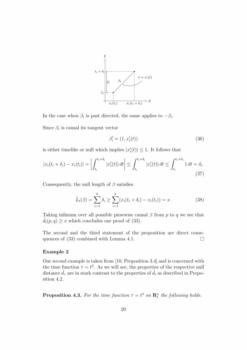
t

xxi(ti)

ti

xi(ti + δi)

ti + δi

βiδi

x = xi(t)

In the case when βi is past directed, the same applies to −βi.

Since βi is causal its tangent vector

β′i = (1, x′i(t)) (36)

is either timelike or null which implies |x′i(t)| ≤ 1. It follows that

|xi(ti + δi)− xi(ti)| =∣∣∣∣∫ ti+δi

ti

|x′i(t)| dt∣∣∣∣ ≤ ∫ ti+δi

ti

|x′i(t)| dt ≤∫ ti+δi

ti

1 dt = δi.

(37)

Consequently, the null length of β satisfies

L̂t(β) =k∑i=1

δi ≥k∑i=1

(xi(ti + δi)− xi(ti)) = x. (38)

Taking infimum over all possible piesewise causal β from p to q we see thatd̂t(p, q) ≥ x which concludes our proof of (33).

The second and the third statement of the proposition are direct conse-quences of (33) combined with Lemma 4.1.

Example 2

Our second example is taken from [10, Proposition 3.4] and is concerned withthe time function τ = t3. As we will see, the properties of the respective nulldistance d̂τ are in stark contrast to the properties of d̂t as described in Propo-sition 4.2.

Proposition 4.3. For the time function τ = t3 on Rn1 the following holds.

20

(1) d̂τ fails to be definite. In particular, for any two points p and q in thet = 0 slice, we have d̂τ (p, q) = 0.

(2) τ̂ fails to encode the causal structure. In particular, for any two pointsp = (tp, ps) and q = (tq, qs), with tp < 0 < tq, we have d̂τ (p, q) =τ(q)− τ(p).

Proof. We assume n = 2 throughout the proof, the case n > 2 is verysimilar. To prove the first claim of the proposition, for any positive integerk we consider a piecewise null curve ηk through p = (T, ps) and q = (T, qs)as shown in the picture:

x

t

pqT

T + l2k

lk

l2k

ηk

Here qs − ps = l and the curve has 2k segments. Clearly, we have

d̂τ (p, q) ≤ L̂τ (ηk) =

((T +

l

2k

)3

− T 3

)· 2k. (39)

Passing to the limit when k →∞ we obtain

d̂τ (p, q) ≤ limk→∞

L̂τ (ηk)

= limk→∞

((T +

l

2k

)3

− T 3

)· 2k

= limk→∞

(T + l

2k

)3 − T 3

l2k· 1l

= limh→0

(T + h

)3 − T 3

h· l =

= ddx

∣∣∣∣x=T

x3 · l

= 3T 2 · l.

(40)

For T = 0 this gives us d̂τ (p, q) ≤ 0. On the other hand, by the definition ofnull distance we have d̂τ (p, q) ≥ 0. It follows that d̂τ (p, q) = 0 for p and q in

21

the t = 0 slice which completes the proof of the first claim.

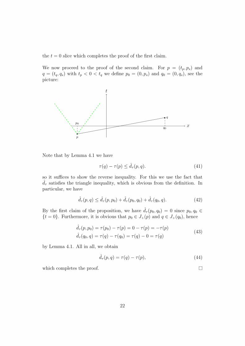
We now proceed to the proof of the second claim. For p = (tp, ps) andq = (tq, qs) with tp < 0 < tq we define p0 = (0, ps) and q0 = (0, qs), see thepicture:

x

t

p

p0

q

q0

Note that by Lemma 4.1 we have

τ(q)− τ(p) ≤ d̂τ (p, q). (41)

so it suffices to show the reverse inequality. For this we use the fact thatd̂τ satisfies the triangle inequality, which is obvious from the definition. Inparticular, we have

d̂τ (p, q) ≤ d̂τ (p, p0) + d̂τ (p0, q0) + d̂τ (q0, q). (42)

By the first claim of the proposition, we have d̂τ (p0, q0) = 0 since p0, q0 ∈{t = 0}. Furthermore, it is obvious that p0 ∈ J+(p) and q ∈ J+(q0), hence

d̂τ (p, p0) = τ(p0)− τ(p) = 0− τ(p) = −τ(p)

d̂τ (q0, q) = τ(q)− τ(q0) = τ(q)− 0 = τ(q)(43)

by Lemma 4.1. All in all, we obtain

d̂τ (p, q) = τ(q)− τ(p), (44)

which completes the proof.

22

5 Conclusion and Discussion

The main purpose of this project was to understand the mathematical foun-dation of the theory of special relativity, focusing on both classical and mod-ern aspects of this subject. In the first part of this project we presented adetailed study of the geometry of Minkowski spacetime. In the second partwe showed how well-known relativistic effects such as the constancy of thespeed of light and the twin paradox can be explained in terms of geometricproperties of Minkowski spacetime. In the third and the last part of thisproject we studied the notion of null distance given by Sormani and Vegain [10] which, for an appropriate choice of a time function, can be used forequipping Minkowski spacetime with metric space structure, encoding alsothe causal structure.

It would be interesting to investigate which properties of a time functionτ make it ”good” in the sense described above and on the contrary ”bad”.The findings of [10], partly presented here, indicate that ”goodness” respec-tively ”badness” is related to non-vanishing respectively vanishing of theLorentzian norm of the gradient |∇τ |. To obtain a complete classificationof time functions on Minkowski spacetime based on the properties of theirrespective null distances would be a first natural step towards understandingthe metric properties of more general spacetimes.

23

References

[1] Loyd S Swenson Jr. The Ethereal Aether: A History of the Michelson-Morley-Miller Aether-Drift Experiments, 1880-1930. University of TexasPress, 2012.

[2] Mark A Handschy. Re-examination of the 1887 Michelson-Morley ex-periment. American Journal of Physics, 50(11):11, 1982.

[3] Gerald Holton. Einstein, Michelson, and the ”Crucial” Experiment. Isis,60(2):133–197, 1969.

[4] John B Kogut. Introduction to Relativity: For Physicists and As-tronomers. Academic Press, 2012.

[5] Barrett O’Neill. Semi-Riemannian Geometry with Applications to Rel-ativity. Academic press, 1983.

[6] Naber L Gregory. The Geometry of Minkowski Space. An Introductionto the Mathematics of the Special Theory of Relativity. Springer–VerlagNew York, Inc, 1992.

[7] Hubert Bray. From Pythagoras to Einstein: The Geometry of Spaceand Time. https://www.youtube.com/watch?v=bkJc373qjsk. PublicLecture, University of Waterloo, 2015.

[8] Gregory J Galloway. Notes on Lorentzian causality. University of Miami,2014.

[9] Dmitri Burago, Iu D Burago, Yuri Burago, Sergei Ivanov, and Sergei AIvanov. A Course in Metric Geometry, volume 33. American Mathe-matical Soc., 2001.

[10] Christina Sormani and Carlos Vega. Null distance on a spacetime. Clas-sical and Quantum Gravity, 33(8):085001, 2016.

24