Mathematical Optimization Models and Methods for …liu.diva-portal.org/smash/get/diva2:442025/FULLTEXT01.pdfLinköping Studies in Science and Technology. Dissertations No. 1396 Mathematical

Linköping Studies in Science and Technology. DissertationsNo. 1396

Mathematical Optimization Modelsand Methods for Open-Pit Mining

Henry Amankwah

Department of MathematicsLinköping University, SE–581 83 Linköping, Sweden

Linköping 2011

Linköping Studies in Science and Technology. DissertationsNo. 1396

Mathematical Optimization Models and Methods for Open-Pit Mining

Henry Amankwah

[email protected]

Department of MathematicsLinköping UniversitySE–581 83 Linköping

Sweden

ISBN 978-91-7393-073-4 ISSN 0345-7524

Copyright c© 2011 Henry Amankwah

Printed by LiU-Tryck, Linköping, Sweden 2011

To Alberta, Grace and Felicia (my mother)

Abstract

Amankwah, H. (2011). Mathematical Optimization Models and Methods forOpen-Pit Mining. Doctoral dissertation.ISBN 978-91-7393-073-4. ISSN 0345-7524.

Open-pit mining is an operation in which blocks from the ground are dug to extract theore contained in them, and in this process a deeper and deeper pit is formed until the min-ing operation ends. Mining is often a highly complex industrial operation, with respectto both technological and planning aspects. The latter may involve decisions about whichore to mine and in which order. Furthermore, mining operations are typically capital in-tensive and long-term, and subject to uncertainties regarding ore grades, future miningcosts, and the market prices of the precious metals contained in the ore. Today, most ofthe high-grade or low-cost ore deposits have already been depleted, and to obtain suffi-cient profitability in mining operations it is therefore today often a necessity to achieveoperational efficiency with respect to both technological and planning issues.

In this thesis, we study the open-pit design problem, the open-pit mining schedulingproblem, and the open-pit design problem with geological and price uncertainty. Theseproblems give rise to (mixed) discrete optimization models that in real-life settings arelarge scale and computationally challenging.

The open-pit design problem is to find an optimal ultimate contour of the pit, givenestimates of ore grades, that are typically obtained from samples in drill holes, estimatesof costs for mining and processing ore, and physical constraints on mining precedenceand maximal pit slope. As is well known, this problem can be solved as a maximum flowproblem in a special network. In a first paper, we show that two well known parametricprocedures for finding a sequence of intermediate contours leading to an ultimate one, canbe interpreted as Lagrangian dual approaches to certain side-constrained design models.In a second paper, we give an alternative derivation of the maximum flow problem of thedesign problem.

We also study the combined open-pit design and mining scheduling problem, which isthe problem of simultaneously finding an ultimate pit contour and the sequence in whichthe parts of the orebody shall be removed, subject to mining capacity restrictions. Thegoal is to maximize the discounted net profit during the life-time of the mine. We showin a third paper that the combined problem can also be formulated as a maximum flowproblem, if the mining capacity restrictions are relaxed; in this case the network howeverneeds to be time-expanded.

In a fourth paper, we provide some suggestions for Lagrangian dual heuristic and timeaggregation approaches for the open-pit scheduling problem. Finally, we study the open-pit design problem under uncertainty, which is taken into account by using the conceptof conditional value-at-risk. This concept enables us to incorporate a variety of possi-ble uncertainties, especially regarding grades, costs and prices, in the planning process.In real-life situations, the resulting models would however become very computationallychallenging.

v

Populärvetenskaplig sammanfattning

Den enklaste formen av brytning av malmkroppar är i dagbrott, vilket innebär att manfrån jordytan skapar en gruva i form av en stor hålighet i berggrunden. Dagbrott kanvara många hundra meter djupa och kilometervida, och även om brytning i dagbrott ärenkel jämfört med underjordsbrytning är det ändå en komplex industriell verksamhet.Detta gäller både med avseende på tekniska lösningar, till exempel val av metallurgiskaprocesser för utvinning av metall ur malmen, och planering av brytningen, till exempelvilken malm som ska brytas och i vilken ordningsföljd. Gruvindustrin är kapitalintensivoch för att skapa lönsamhet krävs både kostnadseffektiva tekniska lösningar och godplanering. Eftersom den malm som bryts idag ofta är mindre värdefull, exempelvis harlägre guldhalter, eller är mer kostnadskrävande än tidigare, exempelvis på grund av störrebrytningsdjup, ställs idag ofta höga krav på teknik och planering för att uppnå lönsamhet.Denna avhandling behandlar teori och metoder för några optimeringsfrågeställningar somuppkommer vid planering av gruvbrytning i dagbrott.

Inför gruvdrift i dagbrott görs provborrningar i berggrunden, ofta i ett rutnät och mednågra hundra meters djup, för att kartlägga malmkroppens utsträckning och för att upp-skatta värdet av malmen i dess olika delar. Utifrån dessa uppgifter görs sedan en diskretis-ering av malmkroppen och berget runtomkring, genom att hela volymen delas in i kuber,eller block, typiskt med en sida på några tiotal meter. För varje block uppskattas förtjän-sten som fås om det skulle brytas genom skattningar av värdet av malmen i blocket ochkostnader för brytning och processering av malmen.

Den första frågeställningen som behandlas i avhandlingen är det mest grundläggandeplaneringsproblemet vid optimering av brytning i dagbrott, nämligen att bestämma vilkablock som ska brytas för att gruvan ska bli maximalt lönsam. För att besvara denna frågaanvänds skattningarna av förtjänsten för varje block, om det bryts, för att konstruera enmatematisk optimeringsmodell som avgör vilka block som ska brytas för att maximeratotala förtjänsten. Modellen innehåller två typer av restriktioner. För det första får dag-brottets väggar inte ha mer än en given maximal lutning, vanligen 45 grader, eftersom deannars rasar. För det andra kan ett block brytas endast om blocken direkt ovanför ocksåbryts. Denna matematiska modell ger den optimala slutliga formen på dagbrottet.

För att göra planeringssituationen mer realistisk är det önskvärt att även ta hänsyn tillatt brytningen i praktiken är utsträckt över en lång tidsrymd, typiskt 10-20 år, och att manvarje år inte kan bryta och processera mer än en viss begränsad mängd malm. Utsträck-ningen i tid gör vidare att det är nödvändigt att beräkna lönsamheten utifrån diskonteradenuvärden av framtida förtjänster. Detta ger upphov till en mer komplicerad optimerings-modell som avgör både vilka block som ska brytas och när. I avhandlingen ges teori ochlösningsmetoder för denna frågeställning.

Gruvbrytning är ofta förknippat med ett stort ekonomiskt risktagande. En orsak tilldetta är geologisk osäkerhet vad gäller värdet på den malm som ska brytas, beroende påatt provborrning endast ger stickprov på värdet. En ytterligare osäkerhet är de framtidapriserna på den metall som utvinns. Eftersom en gruva kräver stora investeringar, oftaunder flera år innan brytningen ska påbörjas, kan dessa osäkerheter leda till en avsevärdekonomisk risk. Det är därför önskvärt att redan på planeringsstadiet ta hänsyn till ochkompensera för osäkerheten. I avhandlingen konstrueras optimeringsmodeller som åstad-kommer detta med hjälp av ett riskmått som har sitt ursprung inom finansmatematiken.

vii

Acknowledgments

I would like to express my sincere gratitude to my main supervisor, Torbjörn Larssonand co-supervisor, Björn Textorius for accepting to work with me. Their encouragement,guidance and support from the initial to the final stage enabled me to develop an under-standing of the subject.

I am most grateful to the Government of Ghana, the University of Cape Coast, andLinköping University for the support they offered me.

I wish to thank Bengt-Ove, Margarita, and Inga-Britt for the time they spent in re-solving some challenges that I went through. I appreciate Zohreh and Aysajan for helpingme with the use of some latex packages. I do acknowledge the help I got from Theresia,Karin, and all the administrative staff of the Department of Mathematics.

I should not forget to say a big thank you to Brian’s family for the encouragementthroughout my stay in Sweden. I would also like to thank Peter for the way and mannerhe accepted and assisted me right from the beginning of my studies, until the time he leftthe department. I am deeply grateful to Hongmei, Lydie, Jolanta, Marcel, Spartak, andJohn (my office mate) for being great friends. They gave me moral support and werealways ever ready to share useful ideas with me. It was really nice and profitable workingwith other colleagues and so they also deserve my thanks. Elin, Pontus, and Kaveh, myneighbours were so kind to me. I would like to take this opportunity to say a big thanksto all of them.

Finally, my special appreciation goes to my family for everything they have done forme.

Linköping, September 15, 2011

Henry Amankwah

ix

Contents

1 Introduction and Overview 11 Open-Pit Design Problem . . . . . . . . . . . . . . . . . . . . . . . . . . 32 Maximum Flow Formulation of the Design Problem . . . . . . . . . . . . 6

2.1 General Maximum Flow Problem . . . . . . . . . . . . . . . . . 62.2 Reformulation of the Design Problem . . . . . . . . . . . . . . . 72.3 An Example . . . . . . . . . . . . . . . . . . . . . . . . . . . . 9

3 Solution Methods for the Design Problem . . . . . . . . . . . . . . . . . 124 Open-Pit Scheduling Problem . . . . . . . . . . . . . . . . . . . . . . . 15

4.1 Models for Scheduling . . . . . . . . . . . . . . . . . . . . . . . 174.2 Adaptations to Large-Scale Mining . . . . . . . . . . . . . . . . 21

5 Uncertainty and Risk . . . . . . . . . . . . . . . . . . . . . . . . . . . . 235.1 Open-Pit Mining Uncertainty . . . . . . . . . . . . . . . . . . . 235.2 Concept of Conditional Value-at-Risk . . . . . . . . . . . . . . . 26

2 Summary of Papers 31

Bibliography 35

Appended Papers 39

I On the use of Parametric Open-Pit Design Models for Mine Scheduling -Pitfalls and Counterexamples 411 Introduction . . . . . . . . . . . . . . . . . . . . . . . . . . . . . . . . . 442 Outline of Picard-Smith Method . . . . . . . . . . . . . . . . . . . . . . 453 Lagrangian Relaxation Interpretation . . . . . . . . . . . . . . . . . . . . 494 Possible Countermeasures . . . . . . . . . . . . . . . . . . . . . . . . . 54

xi

Contents

5 Conclusion . . . . . . . . . . . . . . . . . . . . . . . . . . . . . . . . . 57References. . . . . . . . . . . . . . . . . . . . . . . . . . . . . . . . . . . . . 57

II A Duality-Based Derivation of the Maximum Flow Formulation of the Open-Pit Design Problem 591 Introduction . . . . . . . . . . . . . . . . . . . . . . . . . . . . . . . . . 622 The Mathematical Model . . . . . . . . . . . . . . . . . . . . . . . . . . 633 Derivation of the Maximum Flow Problem . . . . . . . . . . . . . . . . . 634 Conclusion . . . . . . . . . . . . . . . . . . . . . . . . . . . . . . . . . 68References . . . . . . . . . . . . . . . . . . . . . . . . . . . . . . . . . . . . . 68

III A Multi-Parametric Maximum Flow Characterization of the Open-Pit Schedul-ing Problem 711 Introduction . . . . . . . . . . . . . . . . . . . . . . . . . . . . . . . . . 742 The Mathematical Model . . . . . . . . . . . . . . . . . . . . . . . . . . 753 Maximum Flow Problem . . . . . . . . . . . . . . . . . . . . . . . . . . 764 Conclusion . . . . . . . . . . . . . . . . . . . . . . . . . . . . . . . . . 84References . . . . . . . . . . . . . . . . . . . . . . . . . . . . . . . . . . . . . 84

IV Open-Pit Production Scheduling - Suggestions for Lagrangian Dual Heuristicand Time Aggregation Approaches 871 Introduction . . . . . . . . . . . . . . . . . . . . . . . . . . . . . . . . . 902 Notations and a Basic Model . . . . . . . . . . . . . . . . . . . . . . . . 923 Lagrangian Relaxation . . . . . . . . . . . . . . . . . . . . . . . . . . . 934 Procedures for Finding Near-Optimal Solutions . . . . . . . . . . . . . . 955 Experimental Results . . . . . . . . . . . . . . . . . . . . . . . . . . . . 996 Time Aggregation Problem . . . . . . . . . . . . . . . . . . . . . . . . . 1047 A Heuristic Procedure based on Primal-Dual Optimality Conditions . . . 1058 Conclusion and Further Research . . . . . . . . . . . . . . . . . . . . . . 109References . . . . . . . . . . . . . . . . . . . . . . . . . . . . . . . . . . . . . 109

V Open-Pit Mining with Uncertainty - A Conditional Value-at-Risk Approach 1111 Introduction . . . . . . . . . . . . . . . . . . . . . . . . . . . . . . . . . 1142 Problem Formulation . . . . . . . . . . . . . . . . . . . . . . . . . . . . 117

2.1 A CVaR Open-Pit Investment Model . . . . . . . . . . . . . . . . 1182.2 A CVaR Open-Pit Design Model . . . . . . . . . . . . . . . . . . 1202.3 Nested Pit Contours based on CVaR Concept . . . . . . . . . . . 122

3 Numerical Study . . . . . . . . . . . . . . . . . . . . . . . . . . . . . . 1223.1 Test Problem . . . . . . . . . . . . . . . . . . . . . . . . . . . . 1223.2 Number of Scenarios Needed . . . . . . . . . . . . . . . . . . . 1243.3 Results for the Investment Model . . . . . . . . . . . . . . . . . 1263.4 Results for the Design Model . . . . . . . . . . . . . . . . . . . 1303.5 Results for the Nested Pit Contours . . . . . . . . . . . . . . . . 132

4 Conclusion . . . . . . . . . . . . . . . . . . . . . . . . . . . . . . . . . 133References . . . . . . . . . . . . . . . . . . . . . . . . . . . . . . . . . . . . . 133

xii

1Introduction and

Overview

Open-pit mining is a surface mining operation whereby ore, or waste, is excavated fromthe surface of the land. In the process of digging the surface of the land, a deeper anddeeper pit is formed until the mining operation ends. It is usually suitable to determinethe final shape of the pit before the mining operation starts.

The shape and size of an open-pit depend on certain factors which must be under-stood in the planning of the open-pit operation. Some of these factors are bench height,ore recovery, geology, grade and localization of the mineralization, extent of the deposit,topography, property boundaries, production rate, mining cost, processing cost, cutoffgrade and pit slopes (Armstrong, 1990). For example, the bench height, which is the ver-tical distance between each horizontal level of the pit, should be set as high as possiblewithin the limits of the size and type of equipment selected for the desired production.The cutoff grade is any grade that for any specified reason is used to separate any twocourses of action. At any stage of the mining, the operator has to decide whether the nextblock of material should be mined or not. The grade of the block is usually used to makethis decision. The pit slope is one of the major factors that determines the amount ofwaste to be removed so as to mine the ore. For more explanations of these mining terms,see Hustrulid and Kuchta (2006).

The limit of the open-pit must be set at the planning stage. This limit defines theamount of ore that is mined, the metal content and the amount of waste to be removedduring the period of operation. Knowledge gained from designing theultimate pit limitthat maximizes profit is important to all open-pit mining endeavours. Other terms likepitoutline, pit contour, andmaximum closureare used by different authors to describe thefinal pit limit of a mine.

To design an optimal pit, the entire mining volume is partitioned into fixed-size blocks.By using geological information from drill cores, the value of the ore in each block is es-timated. In addition, the cost of mining each block is determined. A profit value can thusbe assigned to each block in the mine. The open-pit minedesign problemis thus, decidingthe blocks of an ore deposit to mine in order to maximize the total profit of the mine, while

1

1 Introduction and Overview

obeying digging constraints on pit slope and constraints thatallow underlying blocks tobe mined only after blocks on top of them.

Any feasible pit outline has a cash value which can be computed. To compute thevalue, we must decide on amining sequenceand then mine out the pit, progressivelyaccumulating the revenues and costs as we go (Whittle, 1990). If we are able to fix theblock values and the slopes then an optimal outline can be determined. An increase inblock values yields that the optimal pit becomes bigger, while an increase in slopes im-plies the optimal pit gets deeper. It is important to calculate the accurate block valuesfor any optimization, because wrong calculations will lead to wrong optimal pit outline.In fact, it is interesting to know that the pit outline and the mining sequence have to beknown in order to compute the block values, particularly if the time value of money isessential, and on the other hand, the block values should be known in order to find theoptimal outline.

For the purpose of optimization, there are two basic rules to be followed when calcu-lating the block values. Firstly, a block value is calculated on the assumption that it hasbeen uncovered and that it will be mined. Secondly, any ongoing cost which would stopif mining were stopped should be included (Whittle, 1990).

Production schedulinghas an effect on the optimal outline. Scheduling an open-pitmeans determining the sequence in which materials of the pit should be removed over thelifetime of the mine and the time interval in which each material is to be mined. This hasan effect on the value of the mine since it determines when various items of revenue andexpenditure will occur. This is essential because the money we have today might lose itsvalue in the coming times.

We usually have “worst case mining” and “best case mining” that are some kind ofsimple mining principles, not based on optimization. The worst case mining is when eachbench is mined completely before the next bench is started. Here, the waste at the pe-riphery of the pit is mined early, and the cost is discounted less than the revenue from thecorresponding ore which is mined much later. The optimal pit for worst case mining isgenerally smaller than is indicated by optimization, by using the present costs and rev-enues. The best case mining is when each bench is mined in turn so that the related oreand waste is mined approximately the same time period. The optimal pit in this case isclose to the one obtained by optimization. The worst case mining can be used when deal-ing with small pits, whereas the best case mining is preferred when dealing with largerpits. There are more opportunities for creative sequencing for the latter.

The selection of a mine design, as described by Abdel Sabouret al. (2008), is basedon estimating net present values of all possible, technically feasible mine plans so as toselect the one with the maximum value. In practice, mine planners cannot know withcertainty the quantity and quality of ore in the ground. This, they term thegeologicaluncertainty. It is recognized among practitioners that mining is a high risk business andthe geological uncertainty is a major source of risk. There are however also other sourcesof uncertainties. The future market behaviour of metal prices and foreign exchange ratesare impossible to be known with certainty, therefore, they are sources of risks affectingmine project profitability. Abdel Sabouret al. (2008) use the termmarket uncertaintyforthese sources of risks and classify them as the second major source of risk. The existenceof uncertainties can thus lead to a high probability that the actual cash flows throughoutthe lifetime of the mining project will be different from those expected. An optimization

2

1 Open-Pit Design Problem

model that maximizes expected return while minimizing risk istherefore important forthe mining sector, as this will help make better decisions on the blocks of ore to mine at aparticular point in time.

Lerchs and Grossmann (1965) are the first to put forward a method to solve the open-pit mine problem. Many researchers have since tried to formulate various optimizationmodels and have developed algorithms to solve the problem. Some researchers have alsomade efforts to solve the problem by applying existing optimization techniques. How-ever, in spite of all the work done, researchers are still looking for better models andalgorithms in this field of study. Newmanet al. (2010) give a literature review based onseveral decades of researches in the field of mine planning. They place emphasis on morerecent work, suggestions for emerging areas, and highlights of successful industry appli-cations.

The purpose of this research work is to develop optimization models and methods inthe area of open-pit mining. The thesis is given in two parts with the outline as follows.The first part is devoted to the introduction and overview of the subject area, followed bya summary of appended papers. The second part is comprised of five appended papers.In Paper I, we give some pitfalls and counterexamples on the use of parametric open-pitdesign models for mine scheduling. A duality-based derivation of the maximum flow for-mulation of the open-pit design problem is the focus of Paper II. This is followed by amulti-parametric maximum flow characterization of the open-pit scheduling problem inPaper III. In Paper IV, we provide some suggestions for Lagrangian dual heuristic andtime aggregation approaches for the open-pit production scheduling problem. In Paper V,the last paper, we study a Conditional Value-at-Risk approach to uncertainty associatedwith open-pit mining.


Picard and Smith (2004) describe the open-pit design problem as a problem of choosingan ultimate contour whose total profit, that is, the sum of the profits of all the blocksin the contour, is maximal among all possible contours. In 1965, Lerchs and Grossmannmade an earliest attempt of solving this problem. They associate a directed node-weightedgraph, called themine graph, with the three-dimensional grid of blocks. They note thatthe maximum profit open-pit mine contour corresponds to a maximum closure in thegraph. A closure in the graph is a subset of the nodes such that if a node belongs to thisset then all its successors also belong to the set, and the closure is maximal if the sum ofnode-weights is maximum.

In order that the walls of an open-pit shall not collapse during mining operations, min-ers are always mindful of how to dig the blocks from the ground. The slope requirementis the main physical constraint in that all blocks on top and preventing the mining of agiven block must be removed. For example, in Figure 1.1, if the safe slope angles areassumed to be45◦ and block 6 is to be removed, then we have to remove blocks 1, 2, and3 as well.

It should be noted that we are only interested in mining the profitable blocks. For eachblock in Figure 1.2, let the values on top be block values and the corresponding numberbelow represent the block label. Then blocks 2, 3, 4, 5, 6, 9, 10, 11, and 16 represent an

3


1 2 3 4

5 6 7 8

9 10 11 12

Figure 1.1: A 2-D block model of a mine.

ultimate pit of blocks where the maximal pit angle is45◦ with a value of 10. Block 15is not profitable to mine because by mining this block we must also mine blocks 1 and 8,and we see that the total value of these blocks is−1. Blocks 2, 3, 4, 5, 9, and 10 representan alternative, and smallest, ultimate pit, since the value of removing blocks 6, 11, and 16is zero and, therefore, contributes nothing. Since the blocks inside an ultimate pit containa profitable amount of ore, they are to be mined.

1_ + 1 +2 1_

2_ 1_ 3+

+ 1 1_

4+ 1_ 2_

_3 2_ + 1 +2 1_ 2_

1 2 43 5 6

7 8 9 10 11 12

13 14 15 16 17 18

Figure 1.2: A 2-D block model of a mine with given block values.

The open-pit design problem can be represented as a graph problem defined on a di-rected graphG = (V,A), whereV is the set of nodes andA is the set of arcs. Each blockcorresponds to a node and is assigned a weight. This weight, which can either be posi-tive or negative, represents the profit value of mining the block (Lerchs and Grossmann,1965). There is a directed arc from nodei to nodej if block i cannot be extracted beforeblock j, which is on a layer immediately above blocki. To decide on the blocks to minein order to maximize profit, a maximum weight set of nodes in the graph such that allsuccessors of all nodes in the set are also included in the set is to be found. As mentionedearlier, this set is the maximum closure of the graph,G.

In order to give a mathematical optimization formulation of the open-pit design prob-lem, we give the following notations. Let

4


V = set of all blocks that can be mined.A = setof pairs(i, j) of blocks such that blockj is a neighbouring

block toi that must be removed before blocki can be mined.ci = cost of mining and processing blocki.ri = revenue obtained from blocki.pi = profit obtained by mining and processing blocki (i.e.,pi = ri − ci).

xi =

{1, if block i is mined0, otherwise.

The revenuesri are estimated by using sampling information from drill holes. The math-ematical optimization model for maximizing the total profit of the mine is therefore givenby

max∑i∈V

pixi

subject to

xi ≤ xj , (i, j) ∈ A

xi ∈ {0, 1}, i ∈ V.

(1.1)

The conditionxi ≤ xj implies that blockj has to be mined before blocki, while obeyingthe pit slope. The setA captures both the slope and the immediate precedence constraints.The constraints of the linear programming relaxation of Model (1.1), where the conditionxi ∈ {0, 1} is replaced by0 ≤ xi ≤ 1, form a unimodular matrix. The linear pro-gramming relaxation therefore possesses the integrality property, in that all the extremepoints are integral (Rhys, 1970). The conditionxi ∈ {0, 1} can therefore be replaced by0 ≤ xi ≤ 1 without changing the optimal objective value.

Consider, for example, the pit in Figure 1.2 and let the block values represent theprofits. Then the associated model is

max−x1 + x2 + 2x3 + . . .+ 3x9 + 4x10 + . . .− x17 − 2x18

subject tox7 ≤ x1

x7 ≤ x2

x8 ≤ x1

x8 ≤ x2

x8 ≤ x3

...x15 ≤ x8

x15 ≤ x9

x15 ≤ x10

...x18 ≤ x11

x18 ≤ x12

xi ∈ {0, 1}, i = 1, . . . , 18.

(1.2)

When we solve the general model (1.1), we get an optimal pit. The outline of this optimal

5


pit is the optimal pit design. So, for the pit in Figure 1.2, the pitcontour is composed ofblocks 2, 3, 4, 5, 6, 9, 10, 11, and 16. However, we often also want information aboutscheduling (which we treat in Section 4) so that we know the order in which the blocksshall be mined.

2 Maximum Flow Formulation of the Design Problem

In this section, we give a general description of the maximum flow problem and a refor-mulation of the open-pit design problem as a maximum flow problem. Furthermore, wegive an example of how to solve the design problem as a maximum flow problem. Finally,we discuss some solution methods.

2.1 General Maximum Flow Problem

For a given directed graph, or network,G = (V,A), with V being the set of nodes andA the set of arcs, a sources and sinkt are added. The source is the start node for a flowthrough the network and the sink is the end node for the flow. Let every arc(i, j) ∈ Abe associated with a capacityu(i, j) ≥ 0 and letv(i, j) be the flow along the arc. It isrequired to associate the valuev(i, j) satisfyingv(i, j) ≤ u(i, j) for each arc,(i, j) ∈ A,such that for every node other thans andt, the sum of the values associated to the arcs thatenter it must equal the sum of the values associated to the arcs that leave it. It is furtherrequired to maximize the sum of the values associated to the arcs leaving the source, andalso entering the sink, which is the total flow in the network. Themaximum flow problemis to find a feasible flow through the network that is maximal.

Now, letN = (V ′, A′) be the network associated withG, whereV ′ = V ∪{s}∪{t}.A cut (S, T ) in the networkN separatings andt is a partition of the nodes ofV ′ withs ∈ S andt ∈ T , S ∪ T = V ′, andS ∩ T = φ. ThecapacityC(S, T ) of the cut(S, T ) isthe sum of the capacities of the arcs over the cut. Thus,

C(S, T ) =∑

i∈S,j∈T

u(i, j). (2.1)

A finite cutis a cut with finite capacity and aminimum cutis a cut of minimum capacityamong all cuts(S, T ). Determining the minimum cut of the networkN is equivalent tofinding the maximum flow inN , from s to t. Ford and Fulkerson (1962) define this as

maxv

f = min(S,T )

C(S, T ), (2.2)

wheref is the value of flow.Ford and Fulkerson (1956) develop an algorithm that computes the maximum flow in

a network. As long as there is a path froms to t, with available capacity on all arcs in thepath, flow is sent along one of these paths. Then another path is found, and so on. A pathwith available capacity is called an augmenting path. To describe the algorithm, it shouldbe noted that the following is maintained after every step in the process:

• v(i, j) ≤ u(i, j), that is, the flow fromi to j does not exceed the capacity.

6


• v(i, j) = −v(j, i), that is, maintaining the net flow betweeni andj. If saya unitsare going fromi to j, andb units fromj to i, thenv(i, j) = a−b andv(j, i) = b−a.

•∑

j∈V v(i, j) = 0, unlessi = s or j = t. That is, the net flow to a node is zero,except for the source, which “produces” flow, and the sink, which “consumes” flow.

This means that the flow through the network is alegal flowafter each round in the al-gorithm. They define theresidual networkNv = (V,A′

v) as the network with capacityuv(i, j) = u(i, j) − v(i, j) and no flow. It should be noted that it is not certain thatA′ = A′

v, as sending flow on arc(i, j) might close(i, j), but open a new arc(j, i) in theresidual network. The algorithm is as follows:

Inputs: GraphN with flow capacityu, sources and sinkt

Output: A flow from s to t which is maximum

1. v(i, j)← 0 for all arcs(i, j) ∈ A′

2. While there is a pathp from s to t in Nv with uv(i, j) > 0 for all (i, j) ∈ p

1. Finduv(p) = min{uv(i, j) | (i, j) ∈ p}2. For each arc(i, j) ∈ p

1. v(i, j)← v(i, j) + uv(p), that is, send flow along the arc2. v(j, i) ← v(j, i) − uv(p), that is, decrease flow along the arc, or, equivalently,

send flow in the backward direction.

The concept described here can be used to solve the open-pit design problem.

2.2 Reformulation of the Design Problem

Picard (1976), using the mine graph augmented with source and sink nodes, finds themaximum closure by solving a maximum flow problem.

To find a maximum closureY ⊂ V , for any given directed graphG = (V,A), whereV represents the set of nodes andA the set of arcs, Picard formulates the problem as a0-1 programming given by

max z =∑i∈V

pixi

subject to

xi ≤ xj , (i, j) ∈ A

xi ∈ {0, 1}, i ∈ V,

(2.3)

wherepi is a weight associated to nodei andxi is a binary variable, which is equal to1 if i ∈ Y and 0 otherwise. In the context of open-pit design the node weight is thenet profit of a block. The conditionxi ≤ xj for (i, j) ∈ A is equivalent to the relationaijxi(xj − 1) = 0, whereaij is the element(i, j) of the incident matrix of the graphG,that is,aij = 1 if (i, j) ∈ A and 0 otherwise. Problem (2.3) can then be written as

7


max z =∑i∈V

pixi

subjectto∑i∈V

∑j∈V

aijxi(xj − 1) = 0

xi ∈ {0, 1}, i ∈ V.

(2.4)

Sinceaijxi(xj − 1) ≤ 0 for all xi ∈ {0, 1} andxj ∈ {0, 1}, Picard deduces that (2.4) isequivalent to

max z =∑i∈V

pixi + λ∑i∈V

∑j∈V

aijxi(xj − 1)

subject to

xi ∈ {0, 1}, i ∈ V,

(2.5)

whereλ is a positive number large enough to ensure that an optimal solution of (2.5)satisfies

∑i∈V

∑j∈V aijxi(xj − 1) = 0, that is, that we have a closure ofG. Picard then

replaces the maximization problem by a minimization problem and finally arrives at anequivalent problem

min f(x) =∑i∈V

(−pixi) +∑i∈V

∑j∈V

λaijxi(1− xj)

subject to

xi ∈ {0, 1}, i ∈ V.

(2.6)

According to Picard, solving (2.6) is equivalent to finding a minimum cut in a relatednetwork. Let the digging constraints of a given mine graphG = (V,A) be such thatblock j ∈ V has to be removed before blocki ∈ V . The closure inG is a set of nodesY ⊂ V such that ifi ∈ Y and(i, j) ∈ A, thenj ∈ Y , that is, it is a subsetY of nodessuch that if a node belongs to the closure then all its successors also belong to the setY .Thevalueof a closureY is given by

v(Y ) =∑

i∈Y

pi. (2.7)

The closure of maximum value is thus a maximum closure. A feasible contour of theopen-pit mine corresponds to a closure in the mine graph, and the open-pit mine designproblem then becomes that of determining the maximum closure in the mine graph (seealso Picard and Smith, 2004). The set of arcs inA′ of the networkN = (V ′, A′), asdefined in Section 2.1, are such that:

Arcs (s, i) with capacityu(s, i) = pi for all i with pi > 0.Arcs (j, t) with capacityu(j, t) = −pj for all j with pj ≤ 0.Arcs (k, l) with capacityu(k, l) =∞ for all arcs(k, l) ∈ A.

Picard establishes that a maximum closure in the graphG corresponds to a minimumcut in the networkN . Further, the relation

8


v(Y ) =∑

i:pi>0

pi − C(S, T ) (2.8)

was established between the value of the closure and the capacity of the correspondingcut.

To solve the open-pit design problem, we form a network related to the mine graph ofthe mine deposit and then solve the maximum flow problem in the network (Picard andSmith, 2004).

2.3 An Example

In this section, we give an example of the maximum flow formulation of the open-pitdesign problem. The derivation of the maximum flow formulation does not follow Picard(1976). Instead, we apply the duality-based derivation presented in Paper II.

x2x1 x3 x4

x5 x6

+1 +1 _1 _1

_12+

Figure 2.1: A 2-D block model of a mine with given profit values.

1 2 3 4

5 6

Figure 2.2: Mine graph of the block model in Figure 2.1.

Consider the two-dimensional block model of a mine with given profit values in Figure2.1. The mine graph corresponding to this block model is given in Figure 2.2. If we thinkof maximizing profit, then we have to solve the associated problem

9


maxx1 + x2 − x3 − x4 + 2x5 − x6

subject to

x5 ≤ x1

x5 ≤ x2

x5 ≤ x3

x6 ≤ x2

x6 ≤ x3

x6 ≤ x4

xi ∈ {0, 1}, i = 1, . . . , 6.

(2.9)

By relaxing the integrality restrictions on the variables and the lower and upper boundconstraints on the variables having positive and negative profit values, respectively, weobtain the problem

maxx1 + x2 − x3 − x4 + 2x5 − x6

subject to

−1 0 0 0 1 00 −1 0 0 1 00 0 −1 0 1 00 −1 0 0 0 10 0 −1 0 0 10 0 0 −1 0 1

x1

x2

x3

x4

x5

x6

≤

000000

x1 ≤ 1, x2 ≤ 1, x5 ≤ 1

−x3 ≤ 0,−x4 ≤ 0,−x6 ≤ 0.(2.10)

Letting yij , wi, andzi, be the dual variables for the three respective sets of constraints,the linear programming dual is given by

minw1 + w2 + w5

subject to

−y51 + w1 = 1−y52 − y62 + w2 = 1−y53 − y63 − z3 = −1−y64 − z4 = −1y51 + y52 + y53 + w5 = 2y62 + y63 + y64 − z6 = −1y51 ≥ 0, y52 ≥ 0, y53 ≥ 0, y62 ≥ 0, y63 ≥ 0, y64 ≥ 0wi ≥ 0, i = 1, 2, 5zi ≥ 0, i = 3, 4, 6,

(2.11)

which can be reformulated as

10


max f

subjectto

vs1 + vs2 + vs5 = f−vs1 − y51 = 0−vs2 − y52 − y62 = 0−y53 − y63 + u3t = 0−y64 + u4t = 0−vs5 + y51 + y52 + y53 = 0y62 + y63 + y64 + u6t = 0−u3t − u4t − u6t = −fy51 ≥ 0, y52 ≥ 0, y53 ≥ 0, y62 ≥ 0, y63 ≥ 0, y64 ≥ 0vsi ≥ 0, i = 1, 2, 5uit ≥ 0, i = 3, 4, 6.

(2.12)

This is a maximum flow problem as shown in Figure 2.3, wheref is total flow,vsi is aflow from a source nodes to a node corresponding to blocki with positive profit value,uit is a flow from a node corresponding to blocki with non-positive profit value to a sinknodet, andyij is a flow from nodei to nodej. The values given on the arcs are theirrespective capacities. Solving the maximum flow problem, we get the result in Figure 2.4,with the optimal flow and capacity shown on each arc.

f fts

1 2 3 4

5 6

vsi uityij

v− v −−− v −

1

1 1

1

12

−

8 8 8

8 8 8

Figure 2.3: A network for the maximum flow problem.

Here, the capacity of the cut separatings from t has the same value as the flow, whichequals 1. This means that (2.2) is fulfilled, so that the flow is maximal and the cut isminimal. To maximize profit for the pit, we therefore have to mine blocks 1, 2, 3, and 5 asshown in Figure 2.5. The maximum profit is 3, whilep1 + p2 + p5 = 4 and the minimumcut capacity is 1, which illustrates the relationship (2.8).

11


ts

1 2 3 4

5 6

f = 1 f = 1

1/2

1/ 8

1/10/1

0/1

0/ 8 0/ 8 0/ 80/ 8

0/ 8

0/1

0/1

CUT

Figure 2.4: A maximum flow and a minimum cut.

x2x1 x3 x4

x5 x6

+1 +1 _1 _1

_12+

Figure 2.5: Final pit shape.

3 Solution Methods for the Design Problem

Lerchs and Grossmann (1965) present an algorithm to determine the optimum design foran open-pit mine. The aim is to design the contour of a pit that maximizes the differencebetween total mine value of the extracted ore and the total cost of extraction of ore andwaste materials. They give the mine graph model of the problem and show that an optimalsolution of the ultimate pit problem is the same as finding the maximum closure of theirmodel.

The mine graphG is first augmented with a dummy nodex0 and dummy arcs(x0, xi).The nodex0 is assigned a negative weight so that it cannot be part of the maximumclosure. A treeT with one distinguished nodex0 (called theroot of T ) is known as arooted tree. The algorithm starts with the construction of a treeT 0 in G. The tree is thentransformed into successive treesT 1, T 2, . . . , Tn following given rules, until no furthertransformation is possible. The maximum closure is then given by the nodes of a set ofwell identified branches of the final tree.

Each arcai of a tree defines abranchTi. The arcai is said tosupportTi. Theweightpi of a branch is the sum of the weights of all nodes of the branch. This weightis associated withai and we say thatai supportsa weightpi. In a treeT with rootx0, a

12

3 Solution Methods for the Design Problem

branchTi is characterized by the orientation of the arcai with respect tox0. The arcaiis called ap-arc (plus-arc) if it points towardTi, that is, if the terminal node ofai is partof Ti. The branchTi then is called ap-branch. If ai points away from the branch then itis called anm-arc(minus-arc) and the branch is anm-branch. A p-arc (branch) isstrongif it supports a weight that is strictly positive. Anm-arc (branch) is strong if it supportsa weight that is zero or negative. Arcs (branches) that are not strong are said to beweak.A nodexi is said to be strong if there exists at least one strong arc on the (unique) pathof T joining xi to the rootx0. Nodes that are not strong are said to be weak. Finally, atree isnormalizedif the rootx0 is common to all strong arcs. The maximum closure of anormalized tree is the set of its strong nodes.

a

b

c

d

e

f

g

h

i

x0

_1_4

_2

_1_4

_4( )+ ,

_3( )+ , _7( ),_

_5( )+ ,

_1( )+ ,

( )+ , 5

_1( )+ ,

( ),_ 1_2( )+ ,

1 2 5

3

Figure 3.1: A mine graph augmented with a dummy nodex0.

a

b

c

d

e

f

g

h

i

x0

_1_4

_2

_1_4

_4( )+ ,

_3( )+ , _7( ),_

_5( )+ ,

_1( )+ ,

( )+ , 5

_1( )+ ,

( ),_ 1_2( )+ ,

1 2 5

3

strong mstrong p

weak p

weak m

Figure 3.2: Strong and weak branches.

To illustrate these concepts, we consider the augmented mine graph in Figure 3.1, whichhas been used by Lerchs and Grossmann and also further explained by Caccetta and Gi-annini (1988). The value assigned to each node is the weight of that node. Each arc islabelled in the form(±, pi) to identify its status. Here, a+ or a− sign represents a p-arcor an m-arc respectively, andpi is the support of the arc. By examining the label of an

13


a

b

c

d

e

f

g

h

i

x0

_1_4

_2

_1_4

1 2 5

3

Figure 3.3: The tree obtained after normalization.

arc we can identify it as strong or weak. The arcs(c, d) and(e, f) are strong, and all theothers are weak. Therefore, nodesa, b, c, f, g, h, andi are strong whiled ande are weak.An illustration of strong and weak branches is given in Figure 3.2. Figure 3.3 is the treeobtained after normalization. We note here that as all dummy arcs are p-arcs, all strongarcs of a normalized tree will also be p-arcs.

The Steps of the algorithm are summarized by Caccetta and Giannini as follows.

Step 1 (Initialization):Construct a normalized treeT 0; T 0 is taken as the spanning tree (a tree of maximal set ofarcs that contains no cycle) whose arc set is{(x0, xi) : xi ∈ V }. Identify the setY 0 ofstrong nodes ofT 0 (which are those nodes with positive weight). Seti = 0 and proceedto Step 2.

Step 2 (Optimality test):Search for an arc(xk, xl) in G such thatxk ∈ Y i andxl /∈ Y i then proceed to Step 3. Ifno such arc is found, stop;Y i is a maximum closure ofG.

Step 3 (Update):Identify the unique(x0, xk)-pathP in T i. Supposex0 is joined toxm in P . Constructthe treeT

′i by replacing the arc(x0, xm) of T i with the arc(xk, xl) and proceed to Step4.

Step 4 (Normalization):Normalize the treeT

′i. This yields a treeT i+1. Identify the setY i+1 of strong verticesof T i+1. Seti+ 1 = i and go to Step 2.

It should be noted that

T′i = T i + (xk, xl)− (x0, xm) (3.1)

The normalized treeT i+1 is obtained by moving along the unique(xm, x0)-path andwhen a strong arc is encountered this arc is deleted andx0 is joined to its branch root.

Picard and Queyranne (1982) give a binary quadratic programming formulation of the

14

4 Open-Pit Scheduling Problem

minimum cut problem and mention that it is of considerable importancein the determi-nation of the optimal contour of an open-pit mine.

Zhao and Kim (1992) present a graph theory oriented algorithm for optimum pit de-sign. Their algorithm produces an optimal solution and maximizes the total undiscountednet profit for a given 3-D block mine model. In terms of the reduction in computationtime and computer memory requirements, they view their algorithm to be of better per-formance as compared to the well known Lerchs and Grossmann Algorithm.

Underwood and Tolwinski (1998) develop a network flow algorithm based on the dualto solve the problem of finding a maximum closure in a mine graph, as studied by Lerchsand Grossmann (1965). They demonstrate that the algorithm is closely related to thatof Lerchs and Grossmann and show how the steps in the algorithm of the latter can beviewed in mathematical programming terms. They show that at any stage of the dualsimplex algorithm the nodes in the union of all strong branches in a tree correspond to thenodes being ‘removed’. The algorithm, they describe, will move from one basic solutionof the dual to another. When considering new arcs to bring into the basis, it is needed onlyto look at arcs joining strong nodes to weak nodes. The goal of their algorithm and that ofLerchs and Grossmann is to find a collection of strong nodes which are feasible. A strongnode is feasible when there are no weak blocks above it which must first be removed inorder to allow access to the block, otherwise, there is a strong node which depends ona weak node. The major difference between the two algorithms is the manner a cycle isbroken for the purpose of attaining a spanning tree. In the case of Underwood and Tol-winski, a cycle is broken by analyzing the change in flow around the cycle. This valueis so chosen to increase this flow as much as possible while maintaining dual feasibility.Lerchs and Grossmann instead use a simple rule for removing the arc. For a detailed de-scription of how this is done, see Underwood and Tolwinski (1998).

Hochbaum and Chen (2000) view the open-pit mining problem as a problem to deter-mine the contours of a mine, based on economic data and engineering feasibility require-ments in order to yield maximum possible net income. They mention that this problemneeds to be solved for very large data sets. They note that in practice, it is necessary to testmultiple scenarios taking into account a variety of realizations of geological predictionsand forecasts of ore value. Even though they view the problem to be equivalent to theminimum cut or maximum flow problem they realize that the industry was experiencingcomputational difficulties in solving the problem. They recognize that the most widelycommonly used algorithm by the mining industry has been the one devised by Lerchsand Grossmann in 1965. They develop a maximum flow “push-relabel” algorithm andcompared it to that of Lerchs and Grossmann. They demonstrate that their algorithm hasa superior performance over the Lerchs and Grossmann algorithm for all types of minedata they tested. However, they admit that the Lerchs and Grossmann algorithm has anadvantage with its more economic use of space and memory, which reduces overhead.


Once the open-pit design problem is solved and the final pit shape is determined, we wantto know the order in which to mine the blocks in the pit. The open-pit mine productionscheduling can be viewed as the sequence by which the blocks of the mine should be

15


removed over the lifetime of the mine in order to maximize the totalprofit from the mine,subject to a set of operational and physical constraints. The optimum pit design plays animportant role in mine scheduling, and it should be at constant review at all stages of thelife of an open-pit.

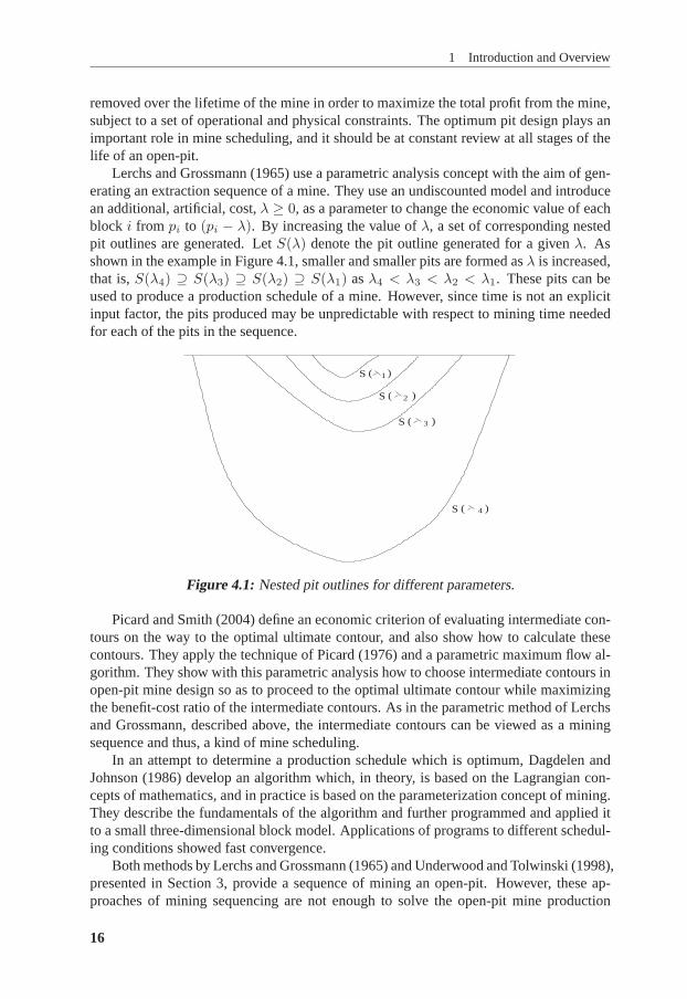
Lerchs and Grossmann (1965) use a parametric analysis concept with the aim of gen-erating an extraction sequence of a mine. They use an undiscounted model and introducean additional, artificial, cost,λ ≥ 0, as a parameter to change the economic value of eachblock i from pi to (pi − λ). By increasing the value ofλ, a set of corresponding nestedpit outlines are generated. LetS(λ) denote the pit outline generated for a givenλ. Asshown in the example in Figure 4.1, smaller and smaller pits are formed asλ is increased,that is,S(λ4) ⊇ S(λ3) ⊇ S(λ2) ⊇ S(λ1) asλ4 < λ3 < λ2 < λ1. These pits can beused to produce a production schedule of a mine. However, since time is not an explicitinput factor, the pits produced may be unpredictable with respect to mining time neededfor each of the pits in the sequence.

S( 1 )

S( )3

S( 2 )

S( )4

Figure 4.1: Nested pit outlines for different parameters.

Picard and Smith (2004) define an economic criterion of evaluating intermediate con-tours on the way to the optimal ultimate contour, and also show how to calculate thesecontours. They apply the technique of Picard (1976) and a parametric maximum flow al-gorithm. They show with this parametric analysis how to choose intermediate contours inopen-pit mine design so as to proceed to the optimal ultimate contour while maximizingthe benefit-cost ratio of the intermediate contours. As in the parametric method of Lerchsand Grossmann, described above, the intermediate contours can be viewed as a miningsequence and thus, a kind of mine scheduling.

In an attempt to determine a production schedule which is optimum, Dagdelen andJohnson (1986) develop an algorithm which, in theory, is based on the Lagrangian con-cepts of mathematics, and in practice is based on the parameterization concept of mining.They describe the fundamentals of the algorithm and further programmed and applied itto a small three-dimensional block model. Applications of programs to different schedul-ing conditions showed fast convergence.

Both methods by Lerchs and Grossmann (1965) and Underwood and Tolwinski (1998),presented in Section 3, provide a sequence of mining an open-pit. However, these ap-proaches of mining sequencing are not enough to solve the open-pit mine production

16


scheduling problem. In practice, we want to construct intermediateoptimal pits and ifpossible, we want to control how these intermediate optimal pits change from one nestedpit to another. If in the construction we have a rapid change in the size of the pit at somestage then we cannot control the sequence of intermediate optimal pit structure. This pos-sibility of a large increment in the size of the pit from one nested pit to the next is knownas the ‘gapping phenomenon’.

4.1 Models for Scheduling

To avoid the situation of encountering the gapping phenomenon, the time factor, as wellas mine capacity constraints on the tonnage to be mined can be introduced explicitly inthe formulation of the open-pit scheduling problem. We begin by defining the followingnotations to be used in the problem formulation. In addition to the notationsV andA inSection 1, let

T = number of time periods.pti = profit derived from mining and processing blocki in time periodt.bi = tonnage of blocki.ut = upper bound on tonnage mined in time periodt.

xti =

{1, if block i is mined in time periodt, or earlier0, otherwise.

A mathematical model for the open-pit scheduling problem then is

maxT∑

t=1

∑i∈V

pti(xti − xt−1

i

)

subject to∑i∈V

bi(xti − xt−1

i

)≤ ut, t = 1, . . . , T

xti ≤ xt

j , (i, j) ∈ A, t = 1, . . . , T

xt−1i ≤ xt

i, t = 1, . . . , T, i ∈ V

x0i = 0, i ∈ V

xti ∈ {0, 1}, i ∈ V, t = 1, . . . , T.

(4.1)

As above, the setA captures both the slope and the immediate precedence constraints, sothat the conditionxt

i ≤ xtj implies that blockj has to be mined if blocki is to be mined,

in time periodt.As an example, consider the pit model in Figure 4.2, which is taken from Lerchs and

Grossmann (1965). For each block, the value on top is the profit and the number at thebottom is the block index. Taking the profits as the initial profits,p0i , and solving thescheduling problem forT = 5, ut = 9, for all t, andbi = 1, for all i, we obtain the resultin Figure 4.3. A discount factor of0.90 is assumed for all the time periods and so theprofit for periodt is computed aspti = 0.90t−1p0i . In Figure 4.3, the number in a blockindicates the time period in which that block is mined.

Caccetta and Hill (2003) present a mixed integer linear programming scheduling for-mulation that distinguishes between ore and waste blocks and that incorporates constraints

17


_4 _4 _4 _4 _4 _4 _4 _4 _4 _4 _4 _4 _4 _4

_4 _4 _4 _4 _4 _4 _4 _4 _4 _4 _4 _4

_4 _4 _4 _4 _4 _4 _4 _4 _4 _4

_4 _4 _4 _4 _4 _4 _4 _4

_4 _4 _4 _4 _4 _4

_4 _4 _4 _4

_4 _4

1122 3 4

5 8 9 106 7

11 12 13 14 15 16 17 18

19 20 21 22 23 24 25 26 27 28

29 30 31 32 33 34 35 36 37 38 39 40

41 42 43 44 45 46 47 48 49 50 51 52 53 54

55 56 57 58 59 60 61 62 63 64 65 66 67 68 69 70

71 72 73 74 75 76 77 78 79 80 81 82 83 84 85 86 87 888 12 12 0

0 12 12 8

8 12 12 0

0 12 12 8

8 12 0

0 12 12 8

8 12 12

0 12 8

12

0

Figure 4.2: A pit model.

11 1 1

1 1

1

22

2

2 2

2

3 3

3 3

3 3

3

3

4

4

4

4

4 5

5

5

51

1

5

5

32

Figure 4.3: Scheduling result forT = 5 andut = 9, for all t.

on mill throughput (mill feed and mill capacity) and volume of material extracted. Theformulation is given as

max z =T∑

t=2

∑i∈V

(pt−1i − pti

)xt−1i +

∑i∈V

pTi xTi (4.2a)

subject to∑i∈Vo

bix1i −m1 = 0 (4.2b)

∑i∈Vo

bi(xti − xt−1

i

)−mt = 0, t = 2, . . . , T (4.2c)

18


∑i∈Vw

bix1i ≤ u1

w (4.2d)

∑i∈Vw

bi(xti − xt−1

i

)≤ ut

w, t = 2, . . . , T (4.2e)

xt−1i ≤ xt

i, t = 2, . . . , T, i ∈ V (4.2f)

xti ≤ xt

j , i ∈ V, (i, j) ∈ A, t = 1, . . . , T (4.2g)

lto ≤ mt ≤ uto, t = 1, . . . , T (4.2h)

xti ∈ {0, 1}, i ∈ V, t = 1, . . . , T, (4.2i)

whereT is again the number of time periods over which the mine is being scheduled,V is the set of blocks (ore or waste),Vo is the set of ore blocks,Vw is the set of wasteblocks,A is the set of precedence arcs,pti is the profit (net present value) resulting fromthe mining of blocki in periodt, bi is the tonnage of blocki, mt is the tonnage of oremilled in periodt, lto is the lower bound on the amount of ore that is milled in periodt, ut

o

is the upper bound on the amount of ore that is milled in periodt, utw is the upper bound

on the amount of waste that is mined in periodt, andxti is a binary variable, which is

equal to 1 if blocki is mined in periods 1 tot and 0 otherwise.Constraints (4.2b), (4.2c) and (4.2h) ensure that the milling capacities hold. Con-

straints (4.2d) and (4.2e) ensure that the tonnage of waste mined does not exceed theprescribed upper bounds. Constraint (4.2f) ensures that a block is mined in one periodonly. Constraint (4.2g) describes the wall slope restrictions. Clearly, this formulation hasa close resemblance to the model to be presented next.

Now, we define auxiliary variablesyti as

yti =

{1, if block i is being mined in periodt0, otherwise.

Thenyti = xti − xt−1

i and the objective becomesmax∑

t

∑i p

tiy

ti . The constraint (4.2f)

means0 = x0i ≤ x1

i ≤ x2i ≤ . . . ≤ xT

i , which is the same as∑

t yti ≤ 1. This means

each block is mined at most once. The fact thatyti is 0 or 1, implies thatyti ≥ 0 and thusxti ≥ xt−1

i , which is constraint (4.2f). Also, we have that∑t

τ=1 yτi = xt

i, t = 1, . . . , T ,and so constraint (4.2g) turns to

∑tτ=1 y

τi ≤

∑tτ=1 y

τj . This implies thatyti ≤

∑tτ=1 y

τj ,

t = 1, . . . , T , (i, j) ∈ A. The formulation (4.2) can thus be restated as

19


maxT∑

t=1

∑i∈V

ptiyti

subject to∑i∈Vo

biyti −mt = 0, t = 1, . . . , T

∑i∈Vw

biyti ≤ ut

w, t = 1, . . . , T

t∑τ=1

yτj − yti ≥ 0, t = 1, . . . , T, (i, j) ∈ A

T∑t=1

yti ≤ 1, i ∈ V

y0i = 0, i ∈ V

lto ≤ mt ≤ uto, t = 1, . . . , T

yti ∈ {0, 1}, i ∈ V, t = 1, . . . , T.

(4.3)

Ferlandet al.(2007) consider the capacitated open-pit mine problem by looking at thesequential extraction of blocks in order to maximize the total discounted profit under anextraction capacity during each period of a planning horizon. As above, letV be the setof blocks in the mining site andA the set of precedence arcs. Further, letpi denote thenet value of extracting blocki, wherei ∈ V , bi denote the tonnage of blocki, i ∈ V , ut

the maximal weight that can be extracted during time periodt, 1 ≤ t ≤ T , and1/(1+α)the discount rate per period. Also, let a binary variablext

i be associated with each blocki for each periodt:

xti =

{1, if block i is being mined in periodt0, otherwise.

Then their formulation of the scheduling block extraction problem is as follows.

maxT∑

t=1

∑i∈V

pi

(1+α)t−1xti (4.4a)

subjectto

T∑t=1

xti ≤ 1, i ∈ V (4.4b)

t∑l=1

xlj − xt

i ≥ 0, t = 1, . . . , T, (i, j) ∈ A (4.4c)

∑i∈V

bixti ≤ ut, t = 1, . . . , T (4.4d)

xti ∈ {0, 1}, i ∈ V, t = 1, . . . , T. (4.4e)

The objective function (4.4a) accounts for the discount factor in evaluating the net valuesof the blocks when they are extracted. Constraint (4.4b) guarantees that each blocki is

20


extracted at most once during the planning horizon. The extractionprecedence is enforcedby constraint (4.4c), and the constraint (4.4d) describes the extraction capacity duringeach period of the horizon.

To initiate the first extraction period,t = 1, we first remove the block among thosehaving no predecessor (i.e., in the top layer) having the largest priority. During any periodt, the next block to be removed is one of those with the highest priority among thosehaving all their predecessors already extracted such that the capacityut is not exceededby its extraction. If no such block exists, then a new extraction period(t+ 1) is initiated.

4.2 Adaptations to Large-Scale Mining

Researchers usually encounter computational difficulties when solving the schedulingproblem of realistic size, because most often, there are too many blocks (over 100,000)within the final pit limits to determine the optimum annual production schedule.

Zhang (2006) approaches the problem of large number of blocks in a mine by com-bining a genetic algorithm and topological sorting to find the extraction schedule of amine. For a given orebody, the approach simultaneously determines an ultimate pit of amine and an optimal block extraction schedule that maximizes the net present value byspecifying whether a block should be extracted and if yes, when to dig it out and where tosend it (i.e., the waste dump or the processing plant), subject to a number of constraintsincluding maximum wall slope, mining and processing capacities.

Genetic algorithms are stochastic, parallel search algorithms based on the theory ofnatural selection and the process of evolution. These algorithms begin with a set of pos-sible solutions randomly selected in the solution space as a population. Each possiblesolution is represented as a chromosome and evaluated for its fitness calculated using anobjective function. Genetic operators such as selection, crossover and mutation are thenapplied to individuals in the current population so as to generate a new population. Theprocess is repeated until an optimal solution, which is the best fitness of any generation,is obtained. A topological sort is an ordering of the nodes of a directed acyclic graph suchthat every edge from a node numberedi to a node numberedj satisfiesi < j. A minegraph is clearly an acyclic graph. Topological sorting is used to randomly select a blockfrom a block model and put it in a queue. The approach starts with an initial population ofchromosomes being created. For each chromosome in the population, topological sortingis performed and a schedule is determined. Next, the chromosomes are evaluated for theirfitness to determine whether or not they have all been processed. If so, then a stoppingcriteria is reached and the process ends, otherwise, genetic algorithm operators to gener-ate a new population are applied and the process is repeated.

Before using such a procedure for production schedule, the blocks of a mine are firstaggregated. Spatially connected blocks with similar properties are predisposed to belongto the same aggregation. Blocks in an aggregation are classified into bins according totheir grades, with blocks in each bin being assumed to be homogeneous in quality. Eachchromosome is comprised of a number of genes, where a gene represents a block aggre-gate. A block aggregate is encoded using the following:

• A random real number which stands for the topological sort preference.

• A decision array where each element represents a bin in the block aggregate and is

21


encoded using a random integer standing for a selected destinationand a randomreal number in(0, 1] representing the proportion of the bin to be sent to the selecteddestination.

Here, destination is where a block bin is sent, whether to the waste dump or to the pro-cessing plant.

A schedule is determined based on the number encoded in the corresponding chro-mosome. Based on the topological sort preference in each block aggregate, topologicalsorting is performed to obtain a feasible extraction sequence of block aggregates satisfy-ing the maximum wall slope constraints. Information from the encoded destination andthe fraction of a block bin to be extracted in each block aggregate determine the totaltonnage for each block aggregate directed to the waste dump and processing plant respec-tively. The extraction time for block aggregates are determined by cutting the extractionsequence of block aggregates into a number of smaller groups retaining the extractionsequence. To evaluate the fitness value of each schedule in a population, Zhang uses theobjective function

NPV =∑

t

∑

k

∑

j

∑

i

Vijkxijkdt, (4.5)

whereVijk is the value of bini of block aggregationj to destinationk, xijk is the fractionof bin i of block aggregationj to destinationk, anddt is the discount factor at timet.

By this approach, Zhang concludes that the computational time can effectively be re-duced whilst maintaining near optimal mine plans. This conclusion was arrived at afteran implementation and an evaluation of the approach against BHP-Billiton’s existing in-dustrial benchmark achieved by the commercial optimizer ILOG CPLEX. Zhang notesthat a difficulty in the use of genetic algorithm to solve the mine planning problem is thatof dealing with the constraints. Two ways are suggested to handle this difficulty. Firstly,the constraints are relaxed and then the violations of constraints are penalized in the ob-jective function. Secondly, the constraints are embedded in chromosome coding and thechromosomes are forced to be feasible in the population. Newmanet al. (2010) point outthat Zhang does not mention the practical consequences of aggregation or how to subse-quently disaggregate.

Ramazan (2007) proposes an algorithm called the “Fundamental Tree Algorithm”,to reduce the number of binary variables required in mixed integer programming (MIP)formulations and the number of constraints within MIP for optimizing annual productionscheduling in open-pit mines. The size of the problem can be reduced by partitioningthe blocks within the final pit limits into smaller volumes called “pushbacks”. Mixed in-teger and linear programming models are recognized as having significant potential foroptimizing production scheduling in open-pit mines, in which the objective is to maxi-mize total discounted profit. However, an MIP formulation of the production schedulingproblem for open-pit mines requires too many binary variables making it very difficultor impossible to solve. For example, if there are 10,000 mining blocks in a pushback tobe scheduled over three years, it will require 30,000 binary variables to generate the MIPformulation. The algorithm of Ramazan involves a newly developed linear programmingmodel formulation to combine blocks into Fundamental Trees. A “Fundamental Tree” isa term used to describe a set of combined blocks, on condition that the combined blocks

22

5 Uncertainty and Risk

have the following three properties.

1. The combined blocks can be mined without violating the slope constraints.

2. The total economic value of the combined blocks is positive.

3. A fundamental tree is maximal in that it cannot be partitioned into smaller treeswithout violating 1 or 2.

All the blocks within the pushback considered for optimization must belong to a funda-mental tree. MIP scheduling formulations of the trees are done by treating each funda-mental tree as a block having certain amount of ore tons with average grade commoditiesand possibly some waste tons. According to Ramazan, a substantial reduction in the MIPproblem size by applying the fundamental tree algorithm reduced the required solutiontime significantly, making it possible to apply MIP models to large open-pit mines.

Bolandet al. (2009) use aggregation with respect to processing, and iterative disag-gregation that refines aggregates up to the point where the refined aggregates defined forprocessing produce the same optimal solution for the linear programming relaxation ofMIP as the optimal solution of the linear programming relaxation with individual blockprocessing. They propose several strategies of creating refined aggregates for the MIPprocessing, using duality results and exploiting the problem structure. They are of theview that these refined aggregates allow the solution of very large problems in reasonabletime with very high solution quality in terms of NPV. They demonstrate their approachusing instances containing as many as 125 aggregates and almost 100,000 blocks.

Bley et al. (2010) consider the integer linear programming formulation presented byCaccetta and Hill (2003). For each time period and each attribute (tonnage of ore andwaste contained within a block), the corresponding production constraint and the prece-dence constraints among the blocks combine to form a precedence constrained knapsackproblem. By exploiting the special structure of such a problem, they derive several typesof additional constraints, whose addition to the standard integer programming formula-tion leads to a tighter linear relaxation and consequently, a reduction of the computationtimes required to solve the production scheduling problems.


There can be uncertainties in the field of mining since the ore values are estimated bythe information from drill holes and it is after the mining process that the returns can beknown. The uncertainty here is due to the fact that we only have samples of blocks. Inthis section, we look at the uncertainty associated with open-pit mining and also introduceConditional Value-at-Risk (CVaR) as a measure to reduce the risk of high losses.

5.1 Open-Pit Mining Uncertainty

For long time horizon open-pit mining, large initial investments and operational budgetsare required. In addition to the historic fluctuations of metal prices, the percentage of orecontained in each block of a deposit is uncertain. These two kinds of uncertainties areknown asprice andgeological uncertainty, respectively. Significant costs are involved

23


in determining ore content with accuracy (Newmanet al., 2010). Miners therefore haveto take risk as the mining operations continue. One of the standard procedures to dealwith uncertainty and risk is to perform the evaluation process for different scenarios ofthe project key variables (Abdel Sabouret al.,2008).

Dimitrakopouloset al. (2002) are the first to introduce the integration of geologicaluncertainty into open-pit mine planning (Abdel Sabouret al.,2008). Dimitrakopoulosetal. are of the view that geological uncertainty as an element in key parameters of open-pitmining projects can be quantified by conditional simulation combined with open-pit op-timization studies. They further claim that having an accurate assessment of uncertaintyarising from grade variability in the ore reserve allows risk in a mining project to be quan-tified and considered in decision-making processes. In their opinion, further technicalintegration of uncertainty in optimization algorithms is needed to enhance the interactionand efficacy of open-pit optimization and risk assessment.

Ramazan and Dimitrakopoulos (2004) note that the mixed integer programming (MIP)approach for optimizing production schedules of open-pit mines has been found to be lim-ited in terms of feasibility in generating optimal solutions with practical mining schedulesand also in its ability to deal within-situ variability of orebodies. They present a produc-tion scheduling method for multi-element deposits in open-pit mines and investigate theissues of infeasibility associated with the traditional MIP models and their limitationswith respect to practical scheduling. They give an alternative formulation that considersthe probability of blocks being scheduled in a given production period, thereby dealingwith in-situ variability and practical issues in scheduling patterns. Their proposed modelgenerates feasible scheduling patterns in terms of practical excavation of the blocks dur-ing the periods they are scheduled. The excavation requires significantly less movementof equipment compared with the schedules produced by the traditional MIP formulation.According to them, since the probability of the blocks being scheduled in a period is con-sidered in the optimization, the new schedule is less risky than the traditional in terms ofmeeting production targets, when considering orebody uncertainty.

As compared to the linear programming (LP) model presented by Dimitrakopoulosand Ramazan (2003) on the same subject, Osanlooet al. (2008) support the fact that theapproach by Ramazan and Dimitrakopoulos is able to maximize the net present value ex-plicitly with the consideration of equipment movements and block access in such a way asto produce a schedule pattern that is less risky than the ones obtained with the traditionalmethods. The LP model by Dimitrakopoulos and Ramazan is noted not to generate max-imum net present value in the presence of grade uncertainty, since the net present valueis not maximized explicitly in their objective function. Osanlooet al. further support theclaim that the approach used by Ramazan and Dimitrakopoulos is able to eliminate par-tial block mining as compared to the method by Dimitrakopoulos and Ramazan, whichschedules some blocks partially and thus contributes to infeasibility or non-optimality ofthe design.

The method by Ramazan and Dimitrakopoulos (2004) however has disadvantageswhich are given by Osanlooet al. (2008) as follows:

• The generation of several scheduling patterns on simulated orebodies is compli-cated and costly.

• The direct integration of grade uncertainty in production planning has not been

24


done. This contributes to the stochastic nature of the grade thatin turn leads toviolating some constraints some periods of time. As a matter of fact the methoddoes not give the best profitable schedule with the minimum possible geologicalrisk.

• Because there may be very significant local deviations between the true grade andsimulated grade, especially in the situation that the drill grid is sparse and wide,detailed mine design on each simulation may result in generating an unrealisticscheduling in the final optimization stage.

• Like all other MIP models for long-term production planning problems, it cannotbe implemented on large deposits.

Dimitrakopoulos and Godoy (2006) present a risk-based, stochastic, approach thatintegrates grade uncertainty into the optimization of long-term production scheduling. Ageneral framework for long-term production scheduling is reviewed and extended throughcombinatorial optimization to allow effective minimization of risk in not achieving pro-duction targets due to geological uncertainty. Their approach first generates a series ofmining schedules, each corresponding to a simulated realization of the spatial distributionof grades. These mining sequences are optimized within a common feasible domain andpost processed to provide a single optimal mining sequence, which minimizes the chanceof deviating from target production figures. The following is the outline of their approach.

1. Derive a stable solution domain of ore production and waste removal stable to allsimulated models of the distribution of grades within the orebody.

2. Determine the optimum production schedule within the solution domain derived inthe first stage above, using a linear programming formulation. This will generateoptimum mining rates for the life-of-mine scheduling.

3. For each one of the simulated models generate a physical mining sequence con-strained to the mining rate derived in the second stage (note that all are sub-optimalmining schedules).

4. Combine, using combinatorial optimization, the mining sequence generated in thethird stage to produce a single optimal mining sequence that minimizes the chanceof deviating from production targets.

Their approach has the ability to minimize deviations from production target variablesto acceptable ranges. For the deterministic approach, the optimization formulation pro-cesses a single estimated orebody model to produce mining schedule. According to them,estimation errors, including the inevitable smoothness of “average” mining block gradeestimates, are propagated to the optimization, because the result is based on imperfect ge-ological knowledge. The final result, as indicated by Dimitrakopouloset al. (2002), is asingle and often biased forecast for the economic outcome of the production schedule. Forthe stochastic framework, geological uncertainties are characterized by a series of equallyprobable models of the orebody, as produced by conditional simulation techniques.

Ramazan and Dimitrakopoulos (2007) consider a stochastic integer programming(SIP) mathematical model that generates optimum long-term production schedules for

25


open-pit mines for a defined objective function, considering theoperational requirementsat the mine. Their model takes multiple simulated orebody models, without averagingthe grades, and maximizes the total net present value when considering geological uncer-tainty caused by grade variability. In the case of production scheduling, the objectives areto maximize the total net present value and to minimize unsatisfied demand for processedore. They incorporate geologic risk discounting concept within the SIP model to controlthe risk distribution between production periods. In their implementation of the model,penalty parameters for deviations from targets are used to control the geological risk dis-tribution in terms of magnitude and variability. The scheduling method developed in theirwork allows the decision-maker to define a risk profile based on the existing uncertaintyquantified by simulated orebody models. In terms of solution time, they consider the SIPmodel to be more efficient compared to the traditional mixed integer programming minescheduling models, as the SIP method contains substantially less binary variables than thelatter. Although they used a hypothetical data set to illustrate the strength of the new SIPmodel, they claim that their model is applicable to large open-pit mines. From their view-point, stochastic programming and modeling concept is useful not only for optimizingthe production scheduling process, but also for investigating various stages of the wholemining process, such as finding the value of an additional drilling.

A popular approach to deal with risk is to apply the conventional Monte Carlo sim-ulation, in which case a distribution for the mine value is obtained rather than a singleexpected value. From this distribution, the risk associated with a long term productionscheduling can be explored by defining the range for the expected value at a certain de-gree of confidence (Abdel Sabouret al., 2008). According to Carneiroet al. (2010), inmany cases it is better to maximize returns with risk constraints. They support the pro-posal of Krokhmalet al.(2002) that, it is better to specify a maximum level of risk. Theseapproaches can be combined in a careful way to formulate design and investment modelsfor the open-pit mine.

5.2 Concept of Conditional Value-at-Risk

We will in this section give a brief introduction to a measure of uncertainty and risk,known as Conditional Value-at-Risk (CVaR), which has its origin within finance. Wegive an example of its use, for portfolio optimization.

Measure of risk plays a critical role in the optimization of portfolios under the pres-ence of uncertainties. Loss can be envisioned as a functionz = f(x, y) of a decision vec-tor x ∈ X ⊂ Rn representing what we may generally call a portfolio, withX expressingdecision constraints, andy ∈ Y ⊂ Rn representing the future values of a number of vari-ables like interest rates or weather data (Rockafellar and Uryasev, 2002). Further, wheny is taken to be random with known probability distribution,z comes out as a randomvariable having its distribution dependent on the choice ofx. Any optimization probleminvolving z in terms of the choice ofx should then take into account not just expectations,but also the “riskiness” ofx.

Value-at-Risk (VaR) is an important measure of risk that is used in the financial in-dustry. Among various risk criteria, is a popular measurement of risk representing thepercentile of the loss distribution with a specified confidence level (Limet al.,2010). Letα ∈ (0, 1) denote the confidence level andf(x, y) a loss function associated with a port-

26


folio x (a vector indicating the fraction of instrument of some available budget in each ofn financialinstruments) and an instrument price (or return) vectory ∈ Rn. [It should benoted thatf(x, y) < 0 means a positive return.] Then, the VaR functionζ(x, α) is givenby the smallest number satisfyingΦ(x, ζ(x, α)) = α, whereΦ(x, ζ) is the probability thatthe lossf(x, y) does not exceed a threshold valueζ, that is,Φ(x, ζ) = Pr[f(x, y) ≤ ζ].So, for any portfoliox ∈ Rn and a confidence levelα, VaR is interpreted as the value ofζ such that the probability of the loss not exceedingζ is α. In simple terms, VaR is themaximum likely loss incurred over a specified period of time at a given confidence level(Lai et al., 2009). The chosen confidence level depends on the purpose of the exerciseand the risk tolerance level of management.

Although the VaR measure is a very popular measure of risk, it has drawbacks, amongthem is lack of consistency, as it violates subadditivity. Nonsubadditivity means that therisk of a portfolio can be higher than the sum of the risks of its individual components.Moreover, in practice, the VaR measure is nonconvex, as well as nondifferentiable, andhence, it is difficult to find global minimum via conventional optimization technique (Limet al.). Furthermore, VaR is difficult to optimize when it is calculated from scenarios. Itis coherent only when it is based on the standard deviation of normal distributions (for anormal distribution VaR is proportional to the standard deviation).

Criticisms of the VaR approach resulted in new proposals for ways to measure risk inportfolios. As an alternative measure, the CVaR was introduced by Rockafellar and Urya-sev (2000) and was further developed by Rockafellar and Uryasev (2002). The CVaRmeasure gives rise to a convex problem and it is considered to be more consistent thanthe VaR. It is defined as the mean loss by which the VaR is exceeded. In other words, theCVaR is the conditional expected loss of a portfolio at a confidence level, given that theloss to be accounted for exceeds or equals the VaR (Carneiroet al.,2010). By definition,the VaR at a given confidence level is never higher than the corresponding CVaR. CVaRis also known asmean excess loss, mean shortfallor tail VaR. Rockafellar and Uryasev(2000) place emphasis on CVaR as an approach to optimizing a portfolio so as to reducethe risk of high losses, even though VaR play a role in this approach. By definition withrespect to a specified probability levelβ, theβ-VaR of a portfolio is the lowest amountα such that, with probabilityβ, the loss will not exceedα, whereas theβ-CVaR is theconditional expectation of losses above that amountα.

Gaivoronski and Pflug (2004/05) present an empirical study of the properties of his-toric VaR and CVaR as functions of portfolio composition using stock market data. Theynote that VaR optimization is nonconvex, exhibits many local minima, and is of combi-natorial character, that is, exhibit exponential growth in computational complexity. Eventhough they argue that computation of mean-VaR efficient portfolios based on historicdata is a feasible task, they confirm that VaR optimization is more difficult than CVaRoptimization.

Lim et al. (2010) are in favour of CVaR. They say that CVaR is a portfolio evalua-tion function having appealing features such as sub-additivity and convexity. Althoughthe CVaR function is nondifferentiable, scenario-based CVaR minimization problems canbe reformulated as linear programs that afford solutions via widely-used commercial soft-wares. However, finding solutions through linear programming formulations for problemshaving many financial instruments and a large number of price scenarios can be time con-suming as the dimension of the problem greatly increases. Anderssonet al. (2001) and

27


Mansiniet al. (2007)support the use of CVaR over VaR.For continuous distributions, CVaR is the conditional expected loss given that the loss

exceeds VaR. That is, CVaR is given by

Φα(x) = (1− α)−1

∫

f(x,y)>ζ(x,α)

f(x, y)p(y)dy, (5.1)

wherep(y) is a probability density function ofy. To avoid complications caused by animplicitly defined functionζ(x, α), Rockafellar and Uryasev (2000) give an alternativefunction

Fα(x, ζ) = ζ + (1− α)−1

∫

f(x,y)>ζ

[f(x, y)− ζ]p(y)dy, (5.2)

for which they show that minimizingFα(x, ζ) with respect to(x, ζ) yields the minimumCVaR and its solution.

When applied to portfolio optimization (Limet al.), xi is the portion of the totalinvestment that is made in a certain security. If the probability distribution ofy is notavailable we can exploit price scenarios, which can be obtained from past price data.Assume that this price data is equally likely (for example, random sampling from a jointprice distribution). For a given price datayj , j = 1, . . . , J , we can approximateFα(x, ζ)by

Fα(x, ζ) = ζ + [(1− α)J ]−1J∑

j=1

max{f j(x)− ζ, 0}, (5.3)

wheref j(x) ≡ f(x, yj). It is well-known thatFα(x, ζ) is a convex function wheneachf j(x) is convex. The functionFα(x, ζ) is noted to be nondifferentiable at(x, ζ)such thatf j(x) − ζ = 0, because then both(∇f j(x)T ,−1)T and0 are subgradients ofmax{f j(x) − ζ, 0}, and since(∇f j(x)T ,−1)T 6= 0, the subdifferential is not a single-ton. A portfolio that minimizes CVaR can be found by considering the nondifferentiableoptimization problem

min ζ + vJ∑

j=1

max{f j(x)− ζ, 0}

subject ton∑

i=1

xi = 1

x ≥ 0, ζ unrestricted.

(5.4)

Here,v ≡ [(1− α)J ]−1.When the loss functionf j(x) is linear, then (5.4) can be solved by using linear pro-

gramming. For a given vector of purchase pricesp ∈ Rn, the linear loss function is givenby f j(x) = (p − yj)Tx. Introducing an auxiliary variable vectorz ∈ RJ , (5.4) can beformulated as the linear programming given by

28


min ζ + vJ∑

j=1

zj

subjectto

zj ≥ (p− yj)Tx− ζ, j = 1, . . . , Jn∑

i=1

xi = 1

x ≥ 0, z ≥ 0, ζ unrestricted.

(5.5)

29

2Summary of Papers

Paper I: On the use of Parametric Open-Pit Design Models forMine Scheduling - Pitfalls and Counterexamples

In this paper, we give an interpretation of the open-pit mining model presented by Picardand Smith (2004), which finds a sequence of intermediate contours leading to an ultimateone, as a Lagrangian relaxation approach. Our aim is to relate their approach to a standardoptimization procedure and standard results, and explain the properties and weaknessesof their approach. We give examples of worst case performance as well as best caseperformance. The worst case behaviour can be very poor in that we might not obtainany scheduling information at all. Our analysis also covers the parametric schedulingapproach of Lerchs and Grossmann (1965), which is closely related to the Picard-Smithapproach.

We show that the two approaches suggested by Lerchs and Grossmann (1965) and Pi-card and Smith (2004) as attempts to obtain scheduling information can be interpreted asLagrangian relaxations of side-constrained versions of the classic open-pit design model.The unpredictable behaviour of the nested pits produced by these approaches, known asthe gapping phenomenon, is observed to be nothing but a manifestation of the lack ofcontrollability that is inherent in Lagrangian relaxation schemes when applied to linearoptimization problems. We further show that it is not the Lagrangian relaxation step initself that creates the gapping phenomenon, since it is still present in the explicitly side-constrained open-pit design model. Furthermore, the side-constrained model does notpossess the nested pit property, which leads to the conclusion that the Lagrangian relax-ation step is crucial for obtaining the nested pit property.

The important deduction from this work is that it seems difficult to avoid the gap-ping phenomenon and obtain proper scheduling information by manipulating the designmodel. Hence, we need to introducetimeexplicitly to get proper scheduling informationfor open-pit mining.

31

2 Summary of Papers

Paper II: A Duality-Based Derivation of the Maximum FlowForm ulation of the Open-Pit Design Problem

In this paper, we formulate the open-pit design problem as a maximum flow problem in acertain capacitated network, as first shown by Picard in 1976. His derivation is based on arestatement of the problem as a quadratic binary program. We give an alternative deriva-tion of the maximum flow formulation, which uses only linear programming duality.

Paper III: A Multi-Parametric Maximum Flow Characterization ofthe Open-Pit Scheduling Problem

We give, in this paper, a multi-parametric maximum flow characterization of the open-pit design and scheduling problem. This is the problem of finding an optimal miningschedule for an open-pit during a number of time periods, subject to mining capacityrestrictions for the time periods. By applying Lagrangian relaxation to the capacities, amulti-parametric formulation is obtained. We show that this formulation can be restatedas a maximum flow problem in a time-expanded network. This result extends the wellknown maximum flow formulation of the open-pit design problem of Picard from 1976to the case of multiple time periods.

Paper IV: Open-Pit Production Scheduling - Suggestions forLagrangian Dual Heuristic and Time Aggregation Approaches

We make suggestions for Lagrangian dual heuristic approaches for the open-pit schedul-ing problem. A Lagrangian relaxation of the problem, which is solvable as a maximumflow problem is presented. Two procedures for finding near-optimal solutions to thescheduling problem are presented. Linear programming relaxations are solved to findvalues of the multipliers for the capacity restrictions to be used in a Lagrangian relaxationof these constraints. It is noted that the solution to the relaxed problem will not in gen-eral satisfy the capacity restrictions. By adjusting the multiplier values of the Lagrangianrelaxation the relaxed solution is forced to become feasible. In order to reduce the com-putational burden of solving the linear programming relaxations of large-scale problems,we suggest using aggregation of the time periods. We further derive a heuristic procedurefor finding near-optimal solutions to the combined open-pit design and scheduling prob-lem of several capacity constraints for each time period. This heuristic is based on newlydeveloped conditions for optimality and near-optimality in general discrete optimizationproblems.

Paper V: Open-Pit Mining with Uncertainty - A ConditionalValue-at-Risk Approach

The selection of a mine design is based on estimating net present values of all possi-ble, technically feasible mine plans so as to select the one with the maximum value. Inpractice, mine planners cannot know with certainty the quantity and quality of ore in theground, and this geological uncertainty is a major source of risk. Furthermore, the futuremarket behaviour of metal prices and foreign exchange rates are impossible to be known

32

with certainty, and therefore, they are also sources of risks affecting mine project prof-itability. Because of these uncertainties, it is recognized among practitioners that miningis a high risk business. An optimization model that maximizes expected return whileminimizing risk is therefore important for the mining sector as this will help make betterdecisions on the blocks of ore to mine at a particular point in time.

We present in this paper a Conditional Value-at-Risk (CVaR) approach to open-pitmining. Value-at-Risk (VaR) is a measure that has been used by the financial institutionsto minimize the loss caused by inadequate monitoring of risk. This measure is noted tohave certain drawbacks such as lack of consistency, nonconvexity, and nondifferentiabil-ity. Rockafellar and Uryasev (2000) introduce the CVaR measure as an alternative to theVaR measure. The CVaR measure gives rise to a convex problem. This measure is furtherdeveloped by Rockafellar and Uryasev (2002).

Our CVaR approach to open-pit mining can take into account both geological andprice uncertainty in the planning. Investment and design models based on this approachare formulated for the open-pit mine. Furthermore, we give a nested pit scheduling modelbased on CVaR. Several numerical results are presented by using scenarios from simu-lated geological and price uncertainties.

33

Bibliography

[1] Abdel Sabour, S. A., Dimitrakopoulos, R. G., and Kumral, M. (2008), Mine DesignSelection under Uncertainty, Mining Technology, Vol. 117, No. 2, pp. 53–64.

[2] Andersson, F., Mausser, H., Rosen, D., and Uryasev, S. (2001), Credit Risk Op-timization with Conditional Value-at-Risk Criterion, Mathematical Programming,Series B, Vol. 89, pp. 273–291.

[3] Armstrong, D. (1990), Definition of Mining Parameters, Surface Mining (2nd Edi-tion), SME-Online DigitalLibrary.

[4] Bley, A., Boland, N., Fricke, C., and Froyland, G. (2010), A Strengthened Formu-lation and Cutting Planes for the Open Pit Mine Production Scheduling Problem,Computers and Operations Research, Vol. 37, pp. 1641–1647.

[5] Boland, N., Dumitrescu, I., Froyland, G., and Gleixner, A. M. (2009), LP-BasedDisaggregation Approaches to Solving the Open Pit Mining Production SchedulingProblem with Block Processing Selectivity, Computers and Operations Research,Vol. 36, pp. 1064–1089.

[6] Caccetta, L. and Giannini, L. M. (1988), An Application of Discrete Mathematics inthe Design of an Open Pit Mine, Discrete Applied Mathematics, Vol. 21, pp. 1–19.

[7] Caccetta, L. and Hill, S. P. (2003), An Application of Branch and Cut to Open PitMine Scheduling, Journal of Global Optimization, Vol. 27, pp. 349–365.

[8] Carneiro, M. C., Ribas, G. P., and Hamacher, S. (2010), Risk Management in the OilSupply Chain: A CVaR Approach, Industrial and Engineering Chemistry Research,Vol. 49, pp. 3286–3294.

35

Bibliography

[9] Dagdelen, K. and Johnson, T. B. (1986), Optimum Open Pit MineProductionScheduling by Lagrangian Parameterization, Application of Computers and Oper-ations Research in the Mineral Industry: 19th AIME, Society of Mining Engineers,Vol. 19, pp. 127–142.

[10] Dimitrakopoulos, R., Farrelly, C., and Godoy, M. C. (2002), Moving Forward fromTraditional Optimisation: Grade Uncertainty and Risk Effects in Open Pit MineDesign, Transactions of the Institute of Mining and Metallurgy, Section A, MiningIndustry, Vol. 111, pp. A82–A89.

[11] Dimitrakopoulos, R. and Ramazan, S. (2003), Managing Risk and Waste Miningin Long-Term Production Planning of Open Pit Mine, SME Annual Meeting andExhibition, pp. 3–151.

[12] Dimitrakopoulos, R. and Godoy, M. (2006), Demand Driven and Risk ManagingStrategic Mine Planning, Minerales, Vol. 60, No. 263, pp. 45–55.

[13] Ferland, J. A., Amaya, J., and Djuimo, M. S. (2007), Particle Swarm Procedure forthe Capacitated Open Pit Mining Problem, Autonomous Robots and Agents, Bookseries: Studies in Computational Intelligence, Springer-Verlag.

[14] Ford, L. R. and Fulkerson, D. R. (1956), Maximum Flow through a Network, Cana-dian Journal of Mathematics, Vol. 8, pp. 399–404.

[15] Ford, L. R. and Fulkerson, D. R. (1962), Flow in Networks, Princeton UniversityPress, NJ.

[16] Gaivoronski, A. A. and Pflug, G. (2004/05), Value-at-Risk in Portfolio Optimization:Properties and Computational Approach, Journal of Risk, Vol. 7, No. 2, pp. 1–31.

[17] Hochbaum, D. and Chen, A. (2000), Performance Analysis and Best Implemen-tations of Old and New Algorithms for the Open-Pit Mining Problem, OperationsResearch, Vol. 48, No. 6, pp. 894–914.

[18] Hustrulid, W. and Kuchta, K. (2006), Open Pit Mine Planning and Design – Volume1: Fundamentals, 2nd Ed., Taylor and Francis.

[19] Krokhmal, P., Palmquist, J., and Uryasev, S. (2002), Portfolio Optimization withConditional Value-at-Risk Objective and Constraints, Journal of Risk, Vol. 4, pp.43–68.

[20] Lai, F. J., Bamford, W. E., Yuen, S. T. S., and Li, T. (2009), Implementing Valueat Risk in Slope Risk Evaluation, International Symposium on Rock Slope Stabilityin Open Pit Mining and Civil Engineering Proceedings 2009, Santiago, Chile, pp.1–10.

[21] Lerchs, H. and Grossmann, I. F. (1965), Optimum Design of Open-Pit Mines, Trans-actions, Canadian Institute of Mining and Metallurgy, Vol. LXVIII, pp. 17–24.

[22] Lim, C., Sherali, H. D., and Uryasev, S. (2010), Portfolio Optimization by Minimiz-ing Conditional Value-at-Risk via Nondifferentiable Optimization, ComputationalOptimization and Applications, Vol. 46, No. 3, pp. 391–415.

36

Bibliography

[23] Mansini, R., Ogryczak, W., and Speranza, M. G. (2007), ConditionalValue at Riskand Related Linear Programming Models for Portfolio Optimization, Annals of Op-erations Research, Vol. 152, pp. 227–256.

[24] Newman, A. M., Rubio, E., Caro, R., Weintraub, A., and Eurek, K. (2010), A Re-view of Operations Research in Mine Planning, Interfaces, Vol. 40, No. 3, pp. 222–245.

[25] Osanloo, M., Gholamnejad, J., and Karimi, B. (2008), Long-Term Open Pit MineProduction Planning: A Review of Models and Algorithms, International Journal ofMining, Reclamation and Environment, Vol. 22, No. 1, pp. 3–35.

[26] Picard, J.-C. (1976), Maximum Closure of a Graph and Applications to Combinato-rial Problems, Management Science, Vol. 22, No. 11, pp. 1268–1272.

[27] Picard, J.-C. and Smith, B. T. (2004), Parametric Maximum Flows and the Calcu-lation of Optimal Intermediate Contours in Open Pit Mine Design, INFOR Journal,Vol. 42, No. 2, pp. 143–153.

[28] Picard, J-C. and Queyranne, M. (1982), Selected Applications of Minimum Cuts inNetworks, Information Systems and Operational Research (INFOR), Vol. 20, No. 4,pp. 394–422.

[29] Ramazan, S. and Dimitrakopoulos, R. (2004), Traditional and New MIP Modelsfor Production Scheduling with In-Situ Grade Variability, International Journal ofSurface Mining, Vol. 18, pp. 85–98.

[30] Ramazan, S. (2007), The New Fundamental Tree Algorithm for Production Schedul-ing of Open Pit Mines, European Journal of Operational Research, Vol. 177, pp.1153–1166.

[31] Ramazan, S. and Dimitrakopoulos, R. (2007), Stochastic Optimization of LongTerm Production Scheduling for Open Pit Mines with a New Integer ProgrammingFormulation, Orebody Modelling and Strategic Mine Planning, The AustralasianInstitute of Mining and Metallurgy, Spectrum Series, Vol. 14, 2nd Edition, pp. 385–391.

[32] Rhys, J. M. W. (1970), A Selection Problem of Shared Fixed Costs and NetworksFlows, Management Science, Vol. 17, No. 3, pp. 200–207.

[33] Rockafellar, R. T. and Uryasev, S. (2000), Optimization of Conditional Value-at-Risk, Journal of Risk, Vol. 2, No. 3, pp. 21–41.

[34] Rockafellar, R. T. and Uryasev, S. (2002), Conditional Value-at-Risk for GeneralLoss Distributions, Journal of Banking and Finance, Vol. 26, No. 7, pp. 1443–1471.

[35] Underwood, R. and Tolwinski, B. (1998), A Mathematical Programming Viewpointfor Solving the Ultimate Pit Problem, European Journal of Operational Research,Vol. 107, pp. 96–107.

37

Bibliography

[36] Whittle, J. (1990), Open Pit Optimization, Surface Mining(2nd Edition), SME-Online Digital Library.

[37] Zhang, M. (2006), Combining Genetic Algorithms and Topological Sort to OptimizeOpen-Pit Mine Plans, Mine Planning and Equipment Selection (MPES) – Cardu, M.,Ciccu, R., Lovera, E. and Michelotti, E. (eds.), Proceedings of 15th InternationalSymposium, pp. 1234–1239.

[38] Zhao, Y. and Kim, Y. C. (1992), A New Optimum Pit Limit Design Algorithm,Application of Computers and Operations Research in the Mineral Industry, Vol.23, pp. 423–434.

38

Documents

Mathematical Optimization Models and Methods for …liu.diva-portal.org/smash/get/diva2:442025/FULLTEXT01.pdfLinköping Studies in Science and Technology. Dissertations No. 1396 Mathematical