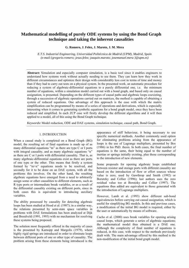
Mathematical modelling of purely ODE systems by using the Bond Graph technique and taking the inherent causalities

G. Romero, J. Felez, J. Maroto, J. M. Mera

E.T.S. Industrial Engineering, Universidad Politécnica de Madrid (UPM), Madrid, Spain

(e-mail:{gregorio.romero; jesus.felez; joaquin.maroto; josemanuel.mera }@upm.es)

Abstract: Simulation and especially computer simulation, is a basic tool since it enables engineers to understand how systems work without actually needing to see them. They can learn how they work in different circumstances and optimize their design with considerably less cost in terms of time and money than if they had to carry out tests on a physical system. In the presented work, an automatic procedure for reducing a system of algebraic-differential equations to a purely differential one, i.e. the minimum number of equations, within a simulation model carried out with a bond graph, and based only on causal assignation, is presented. Depending on the different types of causal paths and algebraic loops coexisting, through a succession of algebraic operations carried out on matrices, the method is capable of obtaining a system of reduced equations. One advantage of this approach is the ease with which the matrix simplification can be programmed by means of a series of operations and derivations, which is especially interesting when it comes to generating symbolic equations for a bond graph model, once they have been reduced and simplified. In each ZCP case will firstly develop the different algorithms and it will then applied to a model, all of this using the Bond Graph technique.

Keywords: Model reduction, ODE and DAE systems, simulation technique, causal path, Bond Graph.

1. INTRODUCTION

When a causal study is completed on a Bond Graph (BG) model, the resulting set of final equations is made up of as many differential equations “m” as there are type C or I ports with integral causality, and as many algebraic equations “n” as there are C or I ports with differential causality. That is, as many algebraic-differential equations exist as there are ports of one type or the other. This means that firstly a system formed by “m+n” equations needs to be resolved, and secondly for it to be done on an DAE system, with all the problems this involves. On the other hand, the resulting algebraic equations have emerged from a need to arbitrarily assign some or other causalities to different elements, such as R type ports or intermediate break variables, or as a result of the differential causality existing on different ports, since in both cases this is equivalent to introducing auxiliary variables.

The ability possessed by causality for detecting algebraic loops has been studied at Hood et al. (1987); in a similar way, the relations presented by semi-state space variables in problems with DAE formulations has been analyzed at Dijk and Breedveld (1991, 1993) with no mechanism for resolving these systems being proposed.

The solution most frequently offered in the majority of cases is the presented by Karnopp and Margolis (1979), where highly rigid springs are introduced in order to eliminate loops between different ports of one or other type of causality. The problem arising from these elements being introduced is the

appearance of stiff behaviour, it being necessary to use specific numerical methods. Another commonly used option for eliminating problems arising from the appearance of loops is the use of Lagrange multipliers, presented by Bos (1986) in his PhD. thesis. In both cases, the final number of equations is the same, their being equal to the number of inertias or springs initially existing, plus those corresponding to the introduction of new elements.

Some proposals for opening algebraic loops established between resistor and storage ports with different causality are based on the introduction of flow or effort sources whose value is zero, used by Gawthrop and Smith (1992) or Borutzky and Cellier (1996); last authors uses the zero residual value too at Borutzky and Cellier (1997). The equations thus added are equivalent to those generated with the introduction of Lagrange multipliers.

However, Lamb et al. (1993) show different sub-bond equivalencies before carrying out causal assignation, which is useful for simplifying BG models. In this and previous cases, a modification of the initial BG model is required, either by the user or automatically by means of software.

Cacho et al. (2000) uses break variables for opening arising causal loops, which generate a series of algebraic equations; the mathematical model thus obtained is a DAE one. Although the complexity of final number of equations is reduced, in this case, with respect to the methods previously dealt with. The main advantage offered by this method is the non-modification of the initial bond graph model.

Birkett and Roe (1989) have researched the method’s mathematical basis, by applying algebraic and matrix theory to resolve general problems set out in BG.

In most cases, when it is wished to simulate a BG model, the problem can usually be resolved by calculating the flows and efforts on the different bonds, at each step of the integration, thereby ignoring the equations represented by the BG.

On other occasions, when the system of equations has been obtained for the model, the numerical values of the different variables and expressions are substituted. We can then resort to specific mathematical methods for operations such as a derivation or integration during the course of the simulation.

This, when added, in some cases to the existence of a series of variable auxiliaries, excessively complicates the simulation, quantitatively as well as qualitatively.

The object of this work, therefore, is, on the one hand, to deduce the final equations of the model without losing sight of the starting parameters, and obtain the equations in a symbolic form where the influence of the different parameters on the different variables can be seen. On the other hand, it is also hoped to obtain the least number of equations, depending only on the degrees of liberty, by means of eliminating the restrictions imposed on the system through a series of matrix operations. In this way, we are working at all times with ODE type systems instead of DAE systems, and the number of numerical algorithms to be used can be increased.

As will be shown in this paper analyzing the different Zero Order Causal Path (ZCP), in order to arrive at the set of final equations, each of the differential causalities or those that have had to be imposed, need to be substituted in bonds or other types of elements by flow or effort sources, and then a series of rules applied in order to gradually form the different algebraic and differential equations that will arise. Once the totality of equations has been formulated, they are reduced, so that the minimum number of equations can be obtained simply by finding their value and then substituting the variables obtained from the algebraic equations for those in the differential equations.

2. BOND GRAPH MODEL WITH ZCPs CLASS 1

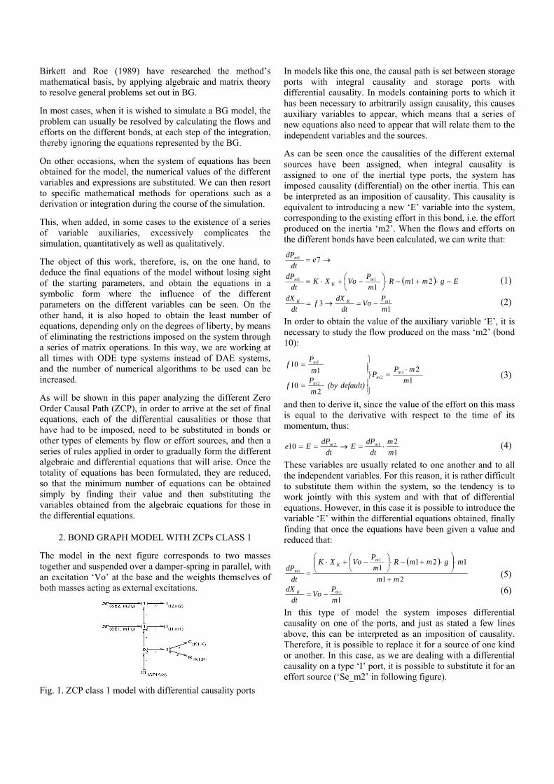
The model in the next figure corresponds to two masses together and suspended over a damper-spring in parallel, with an excitation ‘Vo’ at the base and the weights themselves of both masses acting as external excitations.

Fig. 1. ZCP class 1 model with differential causality ports

In models like this one, the causal path is set between storage ports with integral causality and storage ports with differential causality. In models containing ports to which it has been necessary to arbitrarily assign causality, this causes auxiliary variables to appear, which means that a series of new equations also need to appear that will relate them to the independent variables and the sources.

As can be seen once the causalities of the different external sources have been assigned, when integral causality is assigned to one of the inertial type ports, the system has imposed causality (differential) on the other inertia. This can be interpreted as an imposition of causality. This causality is equivalent to introducing a new ‘E’ variable into the system, corresponding to the existing effort in this bond, i.e. the effort produced on the inertia ‘m2’. When the flows and efforts on the different bonds have been calculated, we can write that:

EgmmRm

PVoXK

dt

dP

edt

dP

mK

m

m

211

7

11

1

(1)

13 1

m

PVo

dt

dXf

dt

dX mKK (2)

In order to obtain the value of the auxiliary variable ‘E’, it is necessary to study the flow produced on the mass ‘m2’ (bond 10):

1

2

210

110

12

2

1

m

mPP

default)(by m

Pf

m

Pf

mm

m

m

(3)

and then to derive it, since the value of the effort on this mass is equal to the derivative with respect to the time of its momentum, thus:

1

210 12

m

m

dt

dPE

dt

dPEe mm (4)

These variables are usually related to one another and to all the independent variables. For this reason, it is rather difficult to substitute them within the system, so the tendency is to work jointly with this system and with that of differential equations. However, in this case it is possible to introduce the variable ‘E’ within the differential equations obtained, finally finding that once the equations have been given a value and reduced that:

21

12111

1

mm

mgmmRm

PVoXK

dt

dPm

K

m

(5)

11

m

PVo

dt

dX mK (6)

In this type of model the system imposes differential causality on one of the ports, and just as stated a few lines above, this can be interpreted as an imposition of causality. Therefore, it is possible to replace it for a source of one kind or another. In this case, as we are dealing with a differential causality on a type ‘I’ port, it is possible to substitute it for an effort source (‘Se_m2’ in following figure).

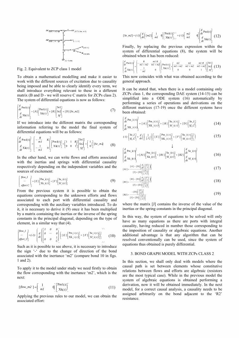
Fig. 2. Equivalent to ZCP class 1 model

To obtain a mathematical modelling and make it easier to work with the different sources of excitation due to causality being imposed and be able to clearly identify every term, we shall introduce everything relevant to these in a different matrix (B and D - we will reserve C matrix for ZCPs class 2). The system of differential equations is now as follows:

ddt

( )Pm1 t

ddt

( )Xk t

[ ]A

( )Pm1 t

( )Xk t[ ]B

Se1

Se2

Sf

[ ]D [ ]Se_m2 (7)

If we introduce into the different matrix the corresponding information referring to the model the final system of differential equations will be as follows:

ddt

( )Pm1 t

ddt

( )Xk t

R

m1K

1m1

0

( )Pm1 t

( )Xk t

1 1 R

0 0 1

Se1

Se2

Sf

1

0[ ]Se_m2 (8)

In the other hand, we can write flows and efforts associated with the inertias and springs with differential causality respectively depending on the independent variables and the sources of excitement:

flow_I ···

effort C [ ] E

( ) Pm_i t ( ) Xk_i t

[ ] F

( ) Se_i t ( ) Sf_i t

(9)

From the previous system it is possible to obtain the equations corresponding to the unknown efforts and flows associated to each port with differential causality and corresponding with the auxiliary variables introduced. To do it, it is necessary to derive it (9) once it has been multiplied by a matrix containing the inertias or the inverse of the spring constants in the principal diagonal, depending on the type of element, in a similar way that (4).

(10)

Such as it is possible to see above, it is necessary to introduce the sign ‘-‘ due to the change of direction of the bond associated with the inertance ‘m2’ (compare bond 10 in figs. 1 and 2).

To apply it to the model under study we need firstly to obtain the flow corresponding with the inertance ‘m2’, which is the next:

(11)

Applying the previous rules to our model, we can obtain the associated effort:

(12)

Finally, by replacing the previous expression within the system of differential equations (8), the system will be obtained when it has been reduced:

ddt

( )Pm1 t

ddt

( )Xk t

Rm1 m2

m1 Km1 m2

1

m10

( )Pm1 t

( )Xk t

m1m1 m2

m1m1 m2

m1 Rm1 m2

0 0 1

Se1

Se2

Sf

(13)

This now coincides with what was obtained according to the general approach.

It can be stated that, when there is a model containing only ZCPs class 1, the corresponding DAE system (14-15) can be simplified into a ODE system (16) automatically by performing a series of operations and derivations on the different matrices (17-19) once the different systems have been obtained:

ddt

( )Pm_i t

ddt

( )XK_i t

[ ]A

( )Pm_i t

( )XK_i t[ ]B

( )Se_i t

( )Sf_i t[ ]D

Se_I

Sf_C

(14)

(-1)

Se_I

Sf_C ddt

1[ ]J

[ ]E

( )Pm_i t

( )XK_i t[ ]F

( )Se_i t

( )Sf_i t

(15)

↓

ddt

( )Pm_i t

ddt

( )Xk_i t

[ ]A1

( )Pm_i t

( )Xk_i t[ ]B1

( )Se_i t

( )Sf_i t[ ]B2

ddt

( )Se_i t

ddt

( )Sf_i t

(16)

[ ]A1[ ]A [ ]D

d

dt

[ ]E[ ]J

[ ]I [ ]D

[ ]E[ ]J

(17)

[ ]B1[ ]B [ ]D

d

dt

[ ]F[ ]J

[ ]I [ ]D

[ ]E[ ]J

(18)

[ ]B2- [ ]D

[ ]F[ ]J

[ ]I [ ]D

[ ]E[ ]J

(19)

where the matrix [J] contains the inverse of the value of the inertias or the spring constants in the principal diagonal.

In this way, the system of equations to be solved will only have as many equations as there are ports with integral causality, having reduced in number those corresponding to the imposition of causality or algebraic equations. Another additional advantage is that any algorithm that can be resolved conventionally can be used, since the system of equations thus obtained is purely differential.

3. BOND GRAPH MODEL WITH ZCPs CLASS 2

In this section, we shall only deal with models where the causal path is set between elements whose constitutive relations between flows and efforts are algebraic (resistors are the most typical case). While in the previous model the system of algebraic equations is obtained performing a derivation, now it will be obtained immediately. In the next model, for a correct causal analysis, a causality needs to be assigned arbitrarily on the bond adjacent to the ‘R2’ resistance.

flow_I

··· effort_C

(-1)·

d d t

I 0 0 0 ··· 0 0 0 1

C

[ ]E

( )Pm_i t ( )XK_i t [ ]F

( )Se_i t ( )Sf_i t

[ ]flow_m2

1m1

0

( )Pm1 t

( )Xk t

[ ]Se_m2 (-1)

d

dt

[ ]m2

1m1

0

( )Pm1 t ( )Xk t (-1)

m2m1

0

ddt

( )Pm1 t

ddt

( )Xk t

As it has been stated in the case studied, this causality is equivalent to introducing a new ‘E’ variable into the system, corresponding to the existing effort in the bond 2.

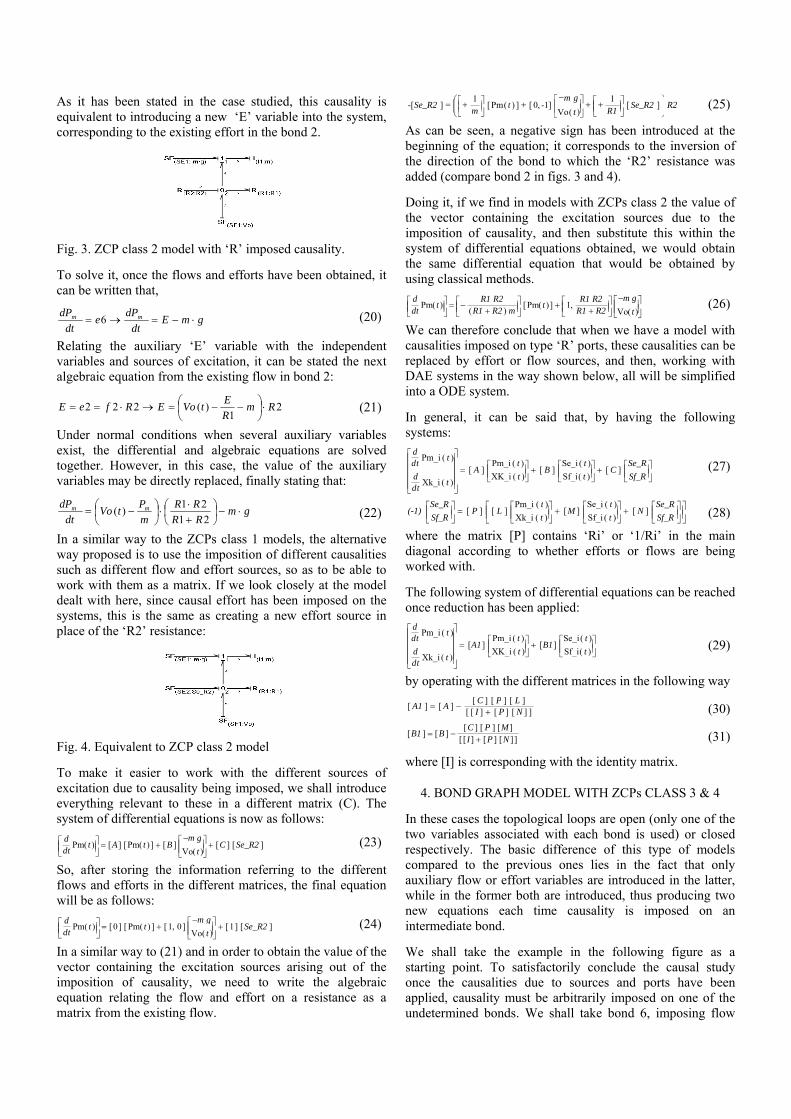
Fig. 3. ZCP class 2 model with ‘R’ imposed causality.

To solve it, once the flows and efforts have been obtained, it can be written that,

gmEdt

dPe

dt

dP mm 6 (20)

Relating the auxiliary ‘E’ variable with the independent variables and sources of excitation, it can be stated the next algebraic equation from the existing flow in bond 2:

21

)(222 RmR

EtVoERfeE

(21)

Under normal conditions when several auxiliary variables exist, the differential and algebraic equations are solved together. However, in this case, the value of the auxiliary variables may be directly replaced, finally stating that:

gmRR

RR

m

PtVo

dt

dP mm

21

21)(

(22)

In a similar way to the ZCPs class 1 models, the alternative way proposed is to use the imposition of different causalities such as different flow and effort sources, so as to be able to work with them as a matrix. If we look closely at the model dealt with here, since causal effort has been imposed on the systems, this is the same as creating a new effort source in place of the ‘R2’ resistance:

Fig. 4. Equivalent to ZCP class 2 model

To make it easier to work with the different sources of excitation due to causality being imposed, we shall introduce everything relevant to these in a different matrix (C). The system of differential equations is now as follows:

d

dt

( )Pm t [ ]A [ ]( )Pm t [ ]B

m g

( )Vo t[ ]C [ ]Se_R2

(23)

So, after storing the information referring to the different flows and efforts in the different matrices, the final equation will be as follows:

d

dt

( )Pm t [ ]0 [ ]( )Pm t [ ],1 0

m g

( )Vo t[ ]1 [ ]Se_R2

(24)

In a similar way to (21) and in order to obtain the value of the vector containing the excitation sources arising out of the imposition of causality, we need to write the algebraic equation relating the flow and effort on a resistance as a matrix from the existing flow.

-[ ]Se_R2

1m

[ ]( )Pm t [ ],0 -1

m g

( )Vo t

1R1

[ ]Se_R2 R2

(25)

As can be seen, a negative sign has been introduced at the beginning of the equation; it corresponds to the inversion of the direction of the bond to which the ‘R2’ resistance was added (compare bond 2 in figs. 3 and 4).

Doing it, if we find in models with ZCPs class 2 the value of the vector containing the excitation sources due to the imposition of causality, and then substitute this within the system of differential equations obtained, we would obtain the same differential equation that would be obtained by using classical methods.

d

dt

( )Pm t

R1 R2( )R1 R2 m

[ ]( )Pm t

,1

R1 R2R1 R2

m g

( )Vo t (26)

We can therefore conclude that when we have a model with causalities imposed on type ‘R’ ports, these causalities can be replaced by effort or flow sources, and then, working with DAE systems in the way shown below, all will be simplified into a ODE system.

In general, it can be said that, by having the following systems:

ddt

( )Pm_i t

ddt

( )Xk_i t

[ ]A

( )Pm_i t

( )XK_i t[ ]B

( )Se_i t

( )Sf_i t[ ]C

Se_R

Sf_R

(27)

(-1)

Se_R

Sf_R[ ]P

[ ]L

( )Pm_i t

( )Xk_i t[ ]M

( )Se_i t

( )Sf_i t[ ]N

Se_R

Sf_R (28)

where the matrix [P] contains ‘Ri’ or ‘1/Ri’ in the main diagonal according to whether efforts or flows are being worked with.

The following system of differential equations can be reached once reduction has been applied:

ddt

( )Pm_i t

ddt

( )Xk_i t

[ ]A1

( )Pm_i t

( )XK_i t[ ]B1

( )Se_i t

( )Sf_i t

(29)

by operating with the different matrices in the following way

[ ]A1 [ ]A[ ]C [ ]P [ ]L

[ ][ ]I [ ]P [ ]N (30) [ ]B1 [ ]B

[ ]C [ ]P [ ]M[ ][ ]I [ ]P [ ]N (31)

where [I] is corresponding with the identity matrix.

4. BOND GRAPH MODEL WITH ZCPs CLASS 3 & 4

In these cases the topological loops are open (only one of the two variables associated with each bond is used) or closed respectively. The basic difference of this type of models compared to the previous ones lies in the fact that only auxiliary flow or effort variables are introduced in the latter, while in the former both are introduced, thus producing two new equations each time causality is imposed on an intermediate bond.

We shall take the example in the following figure as a starting point. To satisfactorily conclude the causal study once the causalities due to sources and ports have been applied, causality must be arbitrarily imposed on one of the undetermined bonds. We shall take bond 6, imposing flow

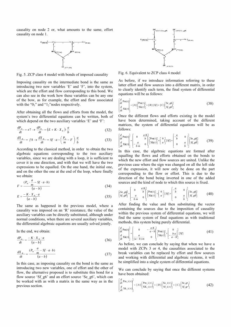
causality on node 2 or, what amounts to the same, effort causality on node 1.

Fig. 5. ZCP class 4 model with bonds of imposed causality

Imposing causality on the intermediate bond is the same as introducing two new variables ‘E’ and ‘F’, into the system, which are the effort and flow corresponding to this bond. We can also see in the work how these variables can be any one of the bow, as for example, the effort and flow associated with the “03” and “12”nodes respectively.

After obtaining all the flows and efforts from the model, the system’s two differential equations can be written, both of which depend on the two auxiliary variables ‘E’ and ‘F’:

b

aXKE

dt

dPe

dt

dPK

mm 7 (32)

b

aF

m

PaSf

dt

dXf

dt

dX mKK

8 (33)

According to the classical method, in order to obtain the two algebraic equations corresponding to the two auxiliary variables, since we are dealing with a loop, it is sufficient to cover it in one direction, and with that we will have the two expressions to be equalled. On the one hand, the initial one, and on the other the one at the end of the loop, where finally we obtain:

ba

baSfm

aP

Fm

)( (34)

ba

aXKE K

(35)

The same as happened in the previous model, where a causality was imposed on an ‘R’ resistance, the value of the auxiliary variables can be directly substituted, although under normal conditions, when there are several auxiliary variables, the differential algebraic equations are usually solved jointly.

In the end, we obtain:

ba

aXK

dt

dP Km

(36)

ba

baSfm

aP

dt

dX mK

)( (37)

In this case, as imposing causality on the bond is the same as introducing two new variables, one of effort and the other of flow, the alternative proposed is to substitute this bond for a flow source ‘Sf_g6’ and an effort source ‘Se_g6’, which can be worked with as with a matrix in the same way as in the previous section.

Fig. 6. Equivalent to ZCP class 4 model

As before, if we introduce information referring to these latter effort and flow sources into a different matrix, in order to clearly identify each term, the final system of differential equations will be as follows:

ddt

( )Pm t

ddt

( )Xk t

[ ]A

( )Pm t

( )Xk t[ ]B [ ]Sf [ ]C

Se_g6

Sf_g6

(38)

Once the different flows and efforts existing in the model have been determined, taking account of the different matrices, the system of differential equations will be as follows:

ddt

( )Pm t

ddt

( )Xk t

0a Kb

a

b m0

( )Pm t

( )Xk t

0

a[ ]Sf

ab

0

0ab

Se_g6

Sf_g6

-

(39)

In this case, the algebraic equations are formed after equalling the flows and efforts obtained on the bonds to which the new effort and flow sources are united. Unlike the previous case where the sign was changed on all the left side of the expression, it will now only be done on the part corresponding to the flow or effort. This is due to the direction of the bond being inverted in one of the added sources and the kind of node to which this source is fixed.

-Se_g6Sf_g6

0a Kb

a

b m0

( )Pm t

( )Xk t

0

a[ ]Sf

ab

0

0ab

Se_g6

Sf_g6

-

(40)

After finding the value and then substituting the vector containing the sources due to the imposition of causality within the previous system of differential equations, we will find the same system of final equations as with traditional methods, this system being purely differential.

ddt

( )Pm t

ddt

( )Xk t

0 a Ka b

a( )a b m

0

( )Pm t

( )Xk t

0

b aa b

[ ]Sf

(41)

As before, we can conclude by saying that when we have a model with ZCPs 3 or 4, the causalities associated to the break variables can be replaced by effort and flow sources and working with differential and algebraic systems, it will be simplified into a single system of differential equations.

We can conclude by saying that once the different systems have been obtained:

ddt

( )Pm_i t

ddt

( )Xk_i t

[ ]A

( )Pm_i t

( )XK_i t[ ]B

( )Se_i t

( )Sf_i t[ ]C

Se_gr

Sf_gr

(42)

[ ]Sgn

Se_gr

Sf_gr [ ]L

( )Pm_i t

( )XK_i t[ ]M

( )Se_i t

( )Sf_i t[ ]N

Se_gr

Sf_gr (43)

where the matrix [Sgn] contains pairs of “±1” in the principal diagonal, the final system of differential equations can be obtained when it has been reduced:

ddt

( )Pm_i t

ddt

( )Xk_i t

[ ]A1

( )Pm_i t

( )XK_i t[ ]B1

( )Se_i t

( )Sf_i t

(44)

simply by operating the different matrices as follows:

[ ]A1 [ ]A[ ]C [ ]L

[ ]Sgn [ ]N (45)

[ ]B1 [ ]B[ ]C [ ]M

[ ]Sgn [ ]N (46)

5. CONCLUSIONS

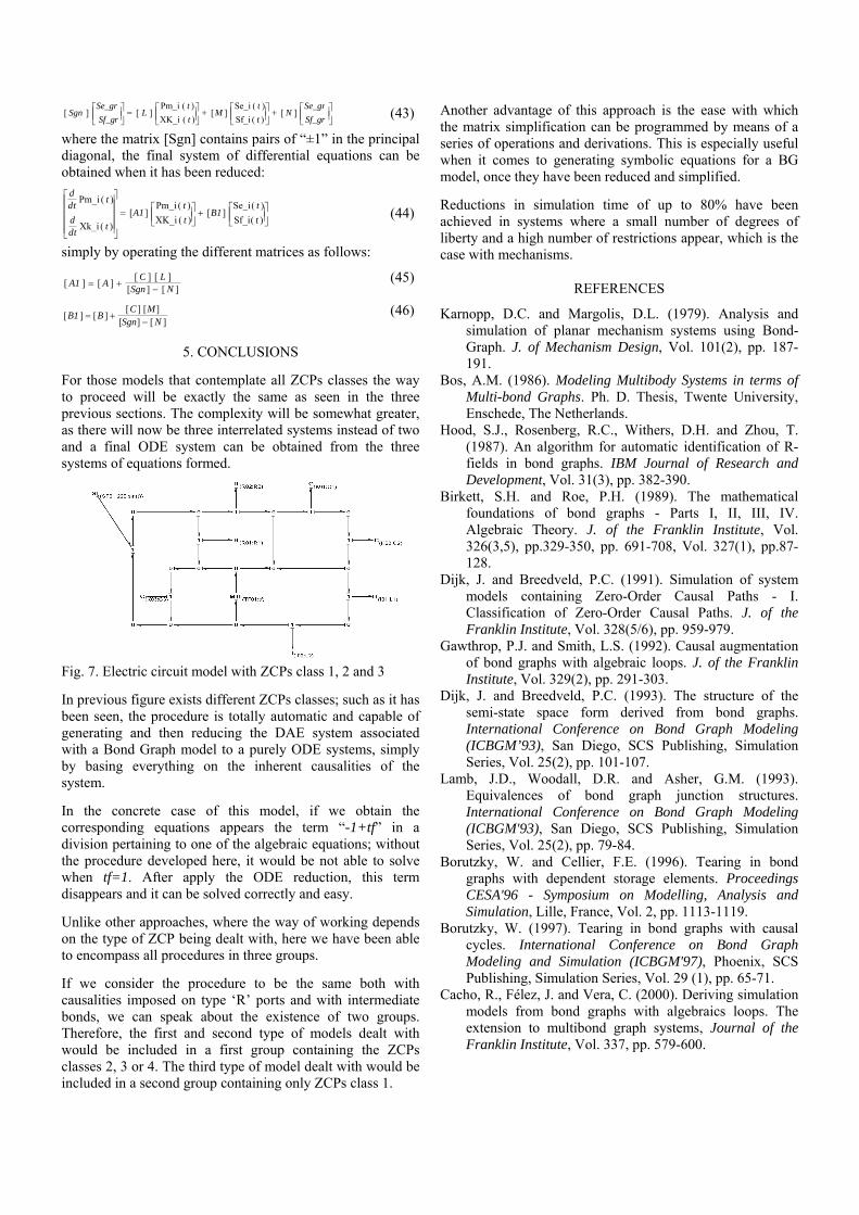
For those models that contemplate all ZCPs classes the way to proceed will be exactly the same as seen in the three previous sections. The complexity will be somewhat greater, as there will now be three interrelated systems instead of two and a final ODE system can be obtained from the three systems of equations formed.

Fig. 7. Electric circuit model with ZCPs class 1, 2 and 3

In previous figure exists different ZCPs classes; such as it has been seen, the procedure is totally automatic and capable of generating and then reducing the DAE system associated with a Bond Graph model to a purely ODE systems, simply by basing everything on the inherent causalities of the system.

In the concrete case of this model, if we obtain the corresponding equations appears the term “-1+tf” in a division pertaining to one of the algebraic equations; without the procedure developed here, it would be not able to solve when tf=1. After apply the ODE reduction, this term disappears and it can be solved correctly and easy.

Unlike other approaches, where the way of working depends on the type of ZCP being dealt with, here we have been able to encompass all procedures in three groups.

If we consider the procedure to be the same both with causalities imposed on type ‘R’ ports and with intermediate bonds, we can speak about the existence of two groups. Therefore, the first and second type of models dealt with would be included in a first group containing the ZCPs classes 2, 3 or 4. The third type of model dealt with would be included in a second group containing only ZCPs class 1.

Another advantage of this approach is the ease with which the matrix simplification can be programmed by means of a series of operations and derivations. This is especially useful when it comes to generating symbolic equations for a BG model, once they have been reduced and simplified.

Reductions in simulation time of up to 80% have been achieved in systems where a small number of degrees of liberty and a high number of restrictions appear, which is the case with mechanisms.

REFERENCES

Karnopp, D.C. and Margolis, D.L. (1979). Analysis and simulation of planar mechanism systems using Bond-Graph. J. of Mechanism Design, Vol. 101(2), pp. 187-191.

Bos, A.M. (1986). Modeling Multibody Systems in terms of Multi-bond Graphs. Ph. D. Thesis, Twente University, Enschede, The Netherlands.

Hood, S.J., Rosenberg, R.C., Withers, D.H. and Zhou, T. (1987). An algorithm for automatic identification of R-fields in bond graphs. IBM Journal of Research and Development, Vol. 31(3), pp. 382-390.

Birkett, S.H. and Roe, P.H. (1989). The mathematical foundations of bond graphs - Parts I, II, III, IV. Algebraic Theory. J. of the Franklin Institute, Vol. 326(3,5), pp.329-350, pp. 691-708, Vol. 327(1), pp.87-128.

Dijk, J. and Breedveld, P.C. (1991). Simulation of system models containing Zero-Order Causal Paths - I. Classification of Zero-Order Causal Paths. J. of the Franklin Institute, Vol. 328(5/6), pp. 959-979.

Gawthrop, P.J. and Smith, L.S. (1992). Causal augmentation of bond graphs with algebraic loops. J. of the Franklin Institute, Vol. 329(2), pp. 291-303.

Dijk, J. and Breedveld, P.C. (1993). The structure of the semi-state space form derived from bond graphs. International Conference on Bond Graph Modeling (ICBGM’93), San Diego, SCS Publishing, Simulation Series, Vol. 25(2), pp. 101-107.

Lamb, J.D., Woodall, D.R. and Asher, G.M. (1993). Equivalences of bond graph junction structures. International Conference on Bond Graph Modeling (ICBGM'93), San Diego, SCS Publishing, Simulation Series, Vol. 25(2), pp. 79-84.

Borutzky, W. and Cellier, F.E. (1996). Tearing in bond graphs with dependent storage elements. Proceedings CESA'96 - Symposium on Modelling, Analysis and Simulation, Lille, France, Vol. 2, pp. 1113-1119.

Borutzky, W. (1997). Tearing in bond graphs with causal cycles. International Conference on Bond Graph Modeling and Simulation (ICBGM'97), Phoenix, SCS Publishing, Simulation Series, Vol. 29 (1), pp. 65-71.

Cacho, R., Félez, J. and Vera, C. (2000). Deriving simulation models from bond graphs with algebraics loops. The extension to multibond graph systems, Journal of the Franklin Institute, Vol. 337, pp. 579-600.