Embed Size (px)
Citation preview
ARTICLE IN PRESS
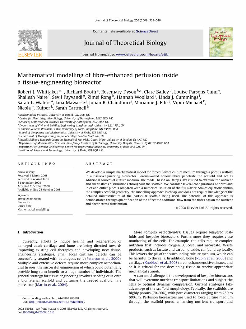
Journal of Theoretical Biology 256 (2009) 533–546
Contents lists available at ScienceDirect
Journal of Theoretical Biology
0022-51
doi:10.1
� Corr
URL
journal homepage: www.elsevier.com/locate/yjtbi
Mathematical modelling of fibre-enhanced perfusion insidea tissue-engineering bioreactor
Robert J. Whittaker a,�, Richard Booth a, Rosemary Dyson b,c, Clare Bailey d, Louise Parsons Chini e,Shailesh Naire f, Sevil Payvandi g, Zimei Rong h, Hannah Woollard c, Linda J. Cummings i,Sarah L. Waters a, Lina Mawasse j, Julian B. Chaudhuri j, Marianne J. Ellis j, Vipin Michael k,Nicola J. Kuiper k, Sarah Cartmell k
a Mathematical Institute, University of Oxford, OX1 3LB, UKb Centre for Plant Integrative Biology, University of Nottingham, LE12 5RD, UKc School of Mathematical Sciences, University of Nottingham, NG7 2RD, UKd Department of Civil and Building Engineering, Loughborough University, LE11 3TU, UKe Complex Systems Research Center, University of New Hampshire, NH 03824, USAf School of Computing and Mathematics, University of Keele, ST5 5BG, UKg Department of Bioengineering, Imperial College London, SW7 2AZ, UKh Interdisciplinary Research Centre in Biomedical Materials, Queen Mary University of London, E1 4NS, UKi Department of Mathematical Sciences, New Jersey Institute of Technology, University Heights, Newark, NJ 07102-1982, USAj Department of Chemical Engineering, Centre for Regenerative Medicine, University of Bath, BA2 7AY, UKk Institute of Science and Technology, University of Keele, ST4 7QB, UK
a r t i c l e i n f o
Article history:
Received 4 March 2008
Received in revised form
8 September 2008
Accepted 7 October 2008Available online 25 October 2008
Keywords:
Tissue engineering
Bioreactor
Darcy flow
Mathematical modelling
93/$ - see front matter & 2008 Elsevier Ltd. A
016/j.jtbi.2008.10.013
esponding author. Tel.: +441865 280618.
: http://robert.mathmos.net/ (R.J. Whittaker).
a b s t r a c t
We develop a simple mathematical model for forced flow of culture medium through a porous scaffold
in a tissue-engineering bioreactor. Porous-walled hollow fibres penetrate the scaffold and act as
additional sources of culture medium. The model, based on Darcy’s law, is used to examine the nutrient
and shear-stress distributions throughout the scaffold. We consider several configurations of fibres and
inlet and outlet pipes. Compared with a numerical solution of the full Navier–Stokes equations within
the complex scaffold geometry, the modelling approach is cheap, and does not require knowledge of the
detailed microstructure of the particular scaffold being used. The potential of this approach is
demonstrated through quantification of the effect the additional flow from the fibres has on the nutrient
and shear-stress distribution.
& 2008 Elsevier Ltd. All rights reserved.
1. Introduction
Currently, efforts to induce healing and regeneration ofdamaged adult cartilage and bone are being directed towardsimproving existing cell therapies and developing new tissue-engineering strategies. Small focal cartilage defects can besuccessfully treated with autologous cells (Peterson et al., 2000).Multiple and extensive defects require more complex osteochon-dral tissues, the successful engineering of which could potentiallyprovide long-term benefit to a huge number of individuals. Thegeneral strategy for tissue engineering involves seeding cells ontoa biomaterial scaffold and culturing the seeded scaffold in abioreactor (Martin et al., 2004).
ll rights reserved.
More complex osteochondral tissues require bilayered scaf-folds and bespoke bioreactors. Furthermore they require closemonitoring of the cells. For example, the cells require complexnutrition that includes oxygen, glucose, and ascorbate. Wasteproducts, such as lactate and carbon dioxide, can build up locally.This lowers the pH of the surrounding culture medium, which canbe harmful to the cells. In addition, bone (Rubin et al., 2006) andcartilage (Knobloch et al., 2008) are mechanosensitive tissues, andso it is critical for the developing tissue to receive appropriatemechanical stimuli.
A current challenge is the development of bespoke bioreactorsthat will overcome nutrient transport limitations and subject thecells to optimal dynamic compression. Current strategies takeadvantage of the scaffold morphology. Typically, the scaffolds arehighly porous (70–90%), with pore diameters ranging from 250 to600mm. Perfusion bioreactors are used to force culture mediumthrough the scaffold pores, enhancing nutrient transport and
ARTICLE IN PRESS
R.J. Whittaker et al. / Journal of Theoretical Biology 256 (2009) 533–546534
providing mechanical stimuli to the cells (e.g. Abousleimanand Sikavitsas, 2006; Cimetta et al., 2007; Kim et al., 2007).For small tissue-engineered constructs these methods havebeen shown to be successful in comparison to static culture(Glowacki et al., 1998; Goldstein et al., 2001; Bancroft et al., 2002;Cartmell et al., 2003). However, problems arise when the tissuesize is scaled up. Cells residing away from the inlets andoutlets may sit in almost stagnant regions, where both nutrientdelivery and shear stress are compromised. If the centre ofthe construct is to receive adequate flow, then regions near theinlet and outlet may suffer by receiving too much shear stress. Thenon-uniformity of the flow and shear-stress distributions isproblematic.
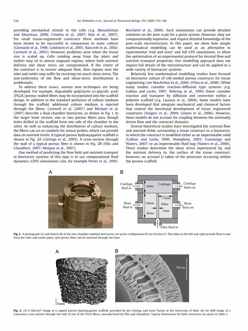
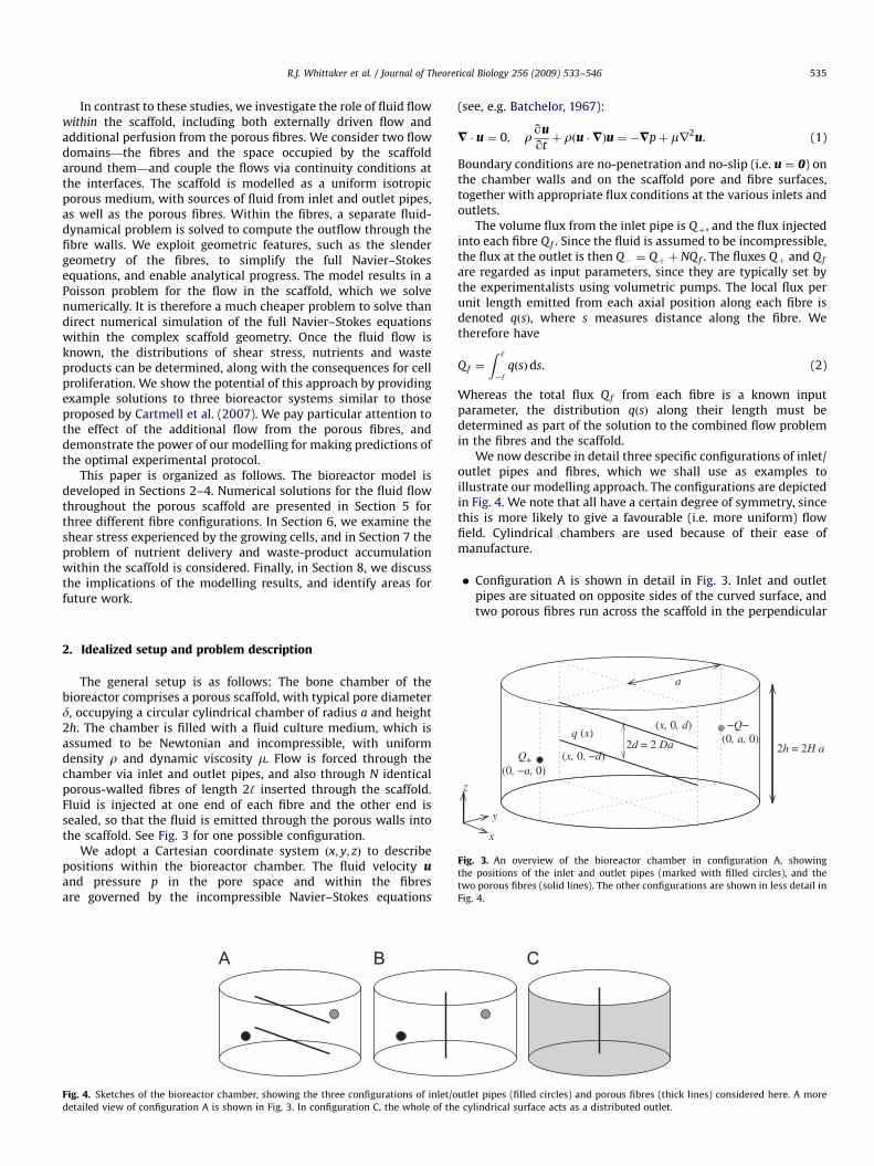
To address these issues, various new techniques are beingdeveloped. For example, degradable poly(lactic-co-glycolic acid)(PLGA) porous-walled fibres may be incorporated into the scaffolddesign. In addition to the standard perfusion of culture mediumthrough the scaffold, additional culture medium is injectedthrough the fibres. Cartmell et al. (2007) and Michael et al.(2007) describe a dual-chamber bioreactor, as shown in Fig. 1. Inthe larger bone section, one or two porous fibres pass thoughholes drilled in the scaffold from one side of the chamber to theother. As well as enhancing the distribution of culture medium,the fibres can act as conduits for sensor probes, which can providedata on nutrient levels. A typical porous hydroxyapatite scaffold isshown in Fig. 2A (Gittings et al., 2005). A cross-section throughthe wall of a typical porous fibre is shown in Fig. 2B (Ellis andChaudhuri, 2007; Morgan et al., 2007).
One method of predicting the flow field and nutrient transportin bioreactor systems of this type is to use computational fluiddynamics (CFD) simulations (see, for example Porter et al., 2005;
Fig. 2. (A) A MicroCT image of a capped porous hydroxyapatite scaffold, provided by
transverse cross-section through the wall of one of the PLGA fibres, manufactured by E
Bfl
Carflu
Fig. 1. A photograph (A) and sketch (B) of the two-chamber modular bioreactor, set up fo
from the inlet and outlet pipes, and porous fibre can be inserted through the base.
Boschetti et al., 2006). Such simulations can provide detailedsolutions on the pore scale for a given system. However, they arecomputationally expensive, and require detailed knowledge of thepore-scale microstructure. In this paper, we show how simplemathematical modelling can be used as an alternative toexperimental ‘trial and error’ and full CFD simulations, to allowthe optimization of an experimental protocol for desired flow andnutrient transport properties. Our modelling approach does notrequire full details of the microstructure and can be applied to awide variety of bioreactor systems.
Relatively few mathematical modelling studies have focusedon bioreactor culture of cell-seeded porous constructs for tissueengineering (see MacArthur et al., 2004; O’Dea et al., 2008). Whilemany studies consider reaction–diffusion type systems (e.g.Galban and Locke, 1997; Nehring et al., 1999) fewer considerreaction and transport by diffusion and convection within apolymer scaffold (e.g. Lasseux et al., 2004). Some models havebeen developed that integrate mechanical and chemical factorsthat control the functional development of tissue engineeredconstructs (Sengers et al., 2004; Lemon et al., 2006). However,these models do not account for coupling between the externallydriven flow and the construct domains.
Several theoretical studies have investigated the external flowand nutrient fields surrounding a tissue construct in a bioreactor,in which the construct is modelled either as an impermeable solid(Galban and Locke, 1999; Humphrey, 2003; Cummings andWaters, 2007) or an impermeable fluid bag (Waters et al., 2006).These studies determine the shear stress experienced by, andthe nutrient delivery to, the surface of the tissue construct;however, no account is taken of the processes occurring withinthe porous scaffold.
Jon Gittings and Irene Turner at the University of Bath. (B) An SEM image of a
llis and Chaudhuri. Typical dimensions for both constructs are given in Table 1.
Fibreoneuid in
Bonefluid out
Fibre fluid in
7.5mm
tilageid in
Cartilagefluid out
Cartilage
10mm
6mm
Bone1mm
r configuration B (see Section 2). The tubes to the left and right provide flow to and
ARTICLE IN PRESS
R.J. Whittaker et al. / Journal of Theoretical Biology 256 (2009) 533–546 535
In contrast to these studies, we investigate the role of fluid flowwithin the scaffold, including both externally driven flow andadditional perfusion from the porous fibres. We consider two flowdomains—the fibres and the space occupied by the scaffoldaround them—and couple the flows via continuity conditions atthe interfaces. The scaffold is modelled as a uniform isotropicporous medium, with sources of fluid from inlet and outlet pipes,as well as the porous fibres. Within the fibres, a separate fluid-dynamical problem is solved to compute the outflow through thefibre walls. We exploit geometric features, such as the slendergeometry of the fibres, to simplify the full Navier–Stokesequations, and enable analytical progress. The model results in aPoisson problem for the flow in the scaffold, which we solvenumerically. It is therefore a much cheaper problem to solve thandirect numerical simulation of the full Navier–Stokes equationswithin the complex scaffold geometry. Once the fluid flow isknown, the distributions of shear stress, nutrients and wasteproducts can be determined, along with the consequences for cellproliferation. We show the potential of this approach by providingexample solutions to three bioreactor systems similar to thoseproposed by Cartmell et al. (2007). We pay particular attention tothe effect of the additional flow from the porous fibres, anddemonstrate the power of our modelling for making predictions ofthe optimal experimental protocol.
This paper is organized as follows. The bioreactor model isdeveloped in Sections 2–4. Numerical solutions for the fluid flowthroughout the porous scaffold are presented in Section 5 forthree different fibre configurations. In Section 6, we examine theshear stress experienced by the growing cells, and in Section 7 theproblem of nutrient delivery and waste-product accumulationwithin the scaffold is considered. Finally, in Section 8, we discussthe implications of the modelling results, and identify areas forfuture work.
x
y
z(0, −a, 0)
Q+
q (x)
(x, 0, −d)2d = 2 Da
(x, 0, d)
a
−Q−(0, a, 0)
2h = 2H a
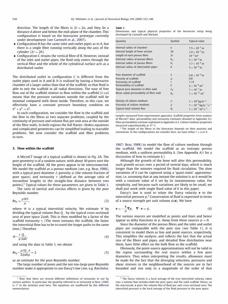
Fig. 3. An overview of the bioreactor chamber in configuration A, showing
the positions of the inlet and outlet pipes (marked with filled circles), and the
two porous fibres (solid lines). The other configurations are shown in less detail in
Fig. 4.
2. Idealized setup and problem description
The general setup is as follows: The bone chamber of thebioreactor comprises a porous scaffold, with typical pore diameterd, occupying a circular cylindrical chamber of radius a and height2h. The chamber is filled with a fluid culture medium, which isassumed to be Newtonian and incompressible, with uniformdensity r and dynamic viscosity m. Flow is forced through thechamber via inlet and outlet pipes, and also through N identicalporous-walled fibres of length 2‘ inserted through the scaffold.Fluid is injected at one end of each fibre and the other end issealed, so that the fluid is emitted through the porous walls intothe scaffold. See Fig. 3 for one possible configuration.
We adopt a Cartesian coordinate system ðx; y; zÞ to describepositions within the bioreactor chamber. The fluid velocity uand pressure p in the pore space and within the fibresare governed by the incompressible Navier–Stokes equations
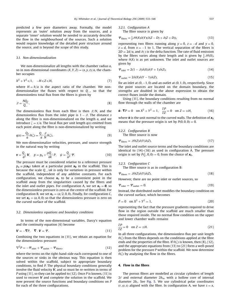
Fig. 4. Sketches of the bioreactor chamber, showing the three configurations of inlet/o
detailed view of configuration A is shown in Fig. 3. In configuration C, the whole of th
(see, e.g. Batchelor, 1967):
= � u ¼ 0; r qu
qtþ rðu �=Þu ¼ �=pþ mr2u. (1)
Boundary conditions are no-penetration and no-slip (i.e. u ¼ 0) onthe chamber walls and on the scaffold pore and fibre surfaces,together with appropriate flux conditions at the various inlets andoutlets.
The volume flux from the inlet pipe is Qþ, and the flux injectedinto each fibre Qf . Since the fluid is assumed to be incompressible,the flux at the outlet is then Q� ¼ Qþ þ NQf . The fluxes Qþ and Qf
are regarded as input parameters, since they are typically set bythe experimentalists using volumetric pumps. The local flux perunit length emitted from each axial position along each fibre isdenoted qðsÞ, where s measures distance along the fibre. Wetherefore have
Qf ¼
Z ‘
�‘qðsÞds. (2)
Whereas the total flux Qf from each fibre is a known inputparameter, the distribution qðsÞ along their length must bedetermined as part of the solution to the combined flow problemin the fibres and the scaffold.
We now describe in detail three specific configurations of inlet/outlet pipes and fibres, which we shall use as examples toillustrate our modelling approach. The configurations are depictedin Fig. 4. We note that all have a certain degree of symmetry, sincethis is more likely to give a favourable (i.e. more uniform) flowfield. Cylindrical chambers are used because of their ease ofmanufacture.
�
utle
e cy
Configuration A is shown in detail in Fig. 3. Inlet and outletpipes are situated on opposite sides of the curved surface, andtwo porous fibres run across the scaffold in the perpendicular
t pipes (filled circles) and porous fibres (thick lines) considered here. A more
lindrical surface acts as a distributed outlet.
ARTICLE IN PRESS
Table 1Dimensions and typical physical properties of the bioreactor setup being
developed by Cartmell and Michael.
Quantity Symbol Typical value
var
is tnom
R.J. Whittaker et al. / Journal of Theoretical Biology 256 (2009) 533–546536
direction. The length of the fibres is 2‘ ¼ 2a, and they lie adistance d above and below the mid-plane of the chamber. Thisconfiguration is based on the bioreactor prototype currentlyunder development (see Cartmell et al., 2007).
�Internal radius of chamber a 7:5� 10�3 m
Internal height of bone section 2h 1:0� 10�2 m
Configuration B has the same inlet and outlet pipes as in A, butthere is a single fibre running vertically along the axis of thecylinder (2‘ ¼ 2h).
Length of each porous fibre 2‘ 10�2 ma
� External radius of porous fibres bw 5� 10�4 mInternal radius of porous fibres bc 1:7� 10�4 m
Internal radius of inlet/outlet pipes d 5� 10�4 m
Pore diameter of scaffold d 6:8� 10�4 m
Porosity of scaffold f 0:8
Tortuosity of scaffold t 1:15
Permeability of scaffold k 2� 10�9 m2
Typical pore diameter in fibre wall dw 1� 10�7 m
Mean radial permeability of fibre wall kw 1� 10�17 m2
Density of culture medium r 1� 103 kg m�3
Viscosity of culture medium m 7� 10�4 kg m�1 s�1
Typical total volume flux Q� 1� 10�7 m3 s�1
Lengths measured from experimental apparatus. Scaffold properties from analysis
of MicroCT data; permeability and tortuosity estimates detailed in Appendix A.1.
Fibre permeability estimate explained in Appendix A.2. Culture medium properties
measured experimentally at 37 �C.a The length of the fibres in the bioreactor depends on their position and
orientation. In the configurations we consider here, we have either ‘ ¼ a or h.
Configuration C retains the vertical fibre of B. However, insteadof the inlet and outlet pipes, the fluid only enters through thevertical fibre and the whole of the cylindrical surface acts as adistributed outlet.
The distributed outlet in configuration C is different from theoutlet pipes used in A and B. It is realized by having a bioreactorchamber of a larger radius than that of the scaffold, so that fluid isable to exit the scaffold in all radial directions. The ease of freeflow out of the scaffold relative to flow within the scaffold (d5a)means that the pressure variations outside the scaffold will beminimal compared with those inside. Therefore, in this case, weeffectively have a constant pressure boundary condition onx2 þ y2 ¼ a2.
In each configuration, we consider the flow in the scaffold andthe flow in the fibres as two separate problems, coupled by thecontinuity of pressure and volume flux per unit area at the outsideof the fibre walls. In both regions the full Navier–Stokes equationsand complicated geometries can be simplified leading to tractableproblems. We now consider the scaffold and fibre problemsin turn.
3. Flow within the scaffold
A MicroCT image of a typical scaffold is shown in Fig. 2A. Thepore geometry is of a random nature, with about 30 pores over theheight of the scaffold. All the pores appear to be interconnected.We model the scaffold as a porous medium (see, e.g. Bear, 1988),with a typical pore diameter d, porosity f (the volume fraction ofpore space), and tortuosity t (defined as the average ratio ofstreamline lengths to the straight-line distance between twopoints).1 Typical values for these parameters are given in Table 1.
The ratio of inertial and viscous effects is given by the poreReynolds number
Rep ¼rUdm , (3)
where U is a typical interstitial velocity. We estimate U bydividing the typical volume flux Q� by the typical cross-sectionalarea of pore space 2fah. This is then modified by a factor of thescaffold tortuosity t. (The more tortuous the scaffold, the fasterthe interstitial flow has to be to travel the longer paths in the sametime.) Therefore
U�tf
Q�2ah
, (4)
and using the data in Table 1, we obtain
Rep�rtQ�d2fahm � 2 (5)
as an estimate for the pore Reynolds number.The large number of pores and the not-too-large pore Reynolds
number make it appropriate to use Darcy’s law (see, e.g. Batchelor,
1 Note that there are several different definitions of tortuosity in use by
ious authors. In particular, the quantity referred to as tortuosity in Bear (1988)2 in the notation used here. The equations are unaffected by this different
enclature.
1967; Bear, 1988) to model the flow of culture medium throughthe scaffold. We model the scaffold as an isotropic porousmedium, with a uniform permeability k. (See Appendix A.1 for adiscussion of how to estimate k.)
Although the growth of the bone will alter this permeability,such growth occurs over a period of several days, which is muchlonger than the minutes required for fluid circulation. The slowvariations of k can be captured using a ‘quasi-static’ approxima-tion, i.e. assuming that at any instant the solution is as it would bewith a constant value of k set by its instantaneous value. Forsimplicity, and because such variations are likely to be small, weshall just work with single fixed value of k in this paper.
Darcy’s law is used to relate the Darcy velocity v to theinterstitial pressure p.2 Conservation of fluid is expressed in termsof a source strength per unit volume cðxÞ. We have
v ¼ �k
m=p; = � v ¼ c. (6)
The various sources are modelled as points and lines and henceappear as delta functions in c. Away from these sources c ¼ 0.
Since the diameter of the porous fibres and the inlet and outletpipes are comparable with the pore size (see Table 1), it isconsistent to model them as line and point sources, respectively.This simplifies the analysis, and reflects the fact that the actualsize of the fibres and pipes, and detailed flow distribution nearthem, have little effect on the bulk flow in the scaffold.
Obviously, the point-source approximations will not be valid inthe region surrounding the real source within a few porediameters. Thus when interpreting the results, allowance mustbe made for the fact that the diverging velocities, pressures andshear stresses in the neighbourhood of the sources are in factbounded and rise only to a magnitude of the order of that
2 The Darcy velocity is a local average of the true interstitial velocity, taken
over a volume that includes both the pore space and the solid scaffold. Hence, on
the macroscale, v gives the volume flux of fluid per unit cross-sectional area. The
interstitial pressure is the local average of the fluid pressure in the pore space.
ARTICLE IN PRESS
R.J. Whittaker et al. / Journal of Theoretical Biology 256 (2009) 533–546 537
predicted a few pore diameters away. Formally, the modelrepresents an ‘outer’ solution away from the sources, and aseparate ‘inner’ solution would be needed to accurately describethe flow in the neighbourhood of the sources. Such a solutionwould require knowledge of the detailed pore structure aroundthe source, and is beyond the scope of this study.
3.1. Non-dimensionalization
We non-dimensionalize all lengths with the chamber radius a,so in non-dimensional coordinates ðX;Y ; ZÞ ¼ ðx; y; zÞ=a, the cham-ber occupies
X2þ Y2p1; �HpZpH, (7)
where H ¼ h=a is the aspect ratio of the chamber. We non-dimensionalize the fluxes with respect to Q�, so that thedimensionless total flux from the fibres is given by
Q ¼NQf
Q�. (8)
The dimensionless flux from each fibre is then Q=N, and thedimensionless flux from the inlet pipe is 1� Q. The distance s
along the fibre is non-dimensionalized on the length a, and weintroduce z ¼ s=a. The local flux per unit length qðsÞ emitted fromeach point along the fibre is non-dimensionalized by writing
qðsÞ ¼Qf
ayðzÞ ¼
Q�a
Q
NyðzÞ. (9)
We non-dimensionalize velocities, pressure, and source strengthin the natural way by writing
v ¼Q�a2
V ; p ¼ p0 þmQ�ak
P; c ¼Q�a3
C. (10)
The pressure must be considered relative to a reference pressurep0 pðx0Þ taken at a particular point x0 in the scaffold. This isbecause the scale Q�=ak is only for variations in pressure withinthe scaffold, independent of any additive constants. For eachconfiguration, we choose x0 to be a convenient point in thescaffold away from the singularities caused by the fibres andthe inlet and outlet pipes. For configuration A, we set x0 ¼ 0, sothe dimensionless pressure is zero at the centre of the scaffold. Forconfiguration B, we set x0 ¼ ða=2;0;0Þ. Finally, for configuration C,we set x0 ¼ ða;0;0Þ so that the dimensionless pressure is zero onthe curved surface of the scaffold.
3.2. Dimensionless equations and boundary conditions
In terms of the non-dimensional variables, Darcy’s equationand the continuity equation (6) become
V ¼ �=P; = � V ¼ C. (11)
Combining the two equations in (11), we obtain an equation forthe dimensionless pressure:
r2P ¼ �Cinlet þCoutlet �Cfibres, (12)
where the terms on the right-hand-side each correspond to one ofthe sources or sinks in the obvious way. This equation is thensolved within the scaffold, subject to appropriate boundaryconditions, to find P. The physical boundary conditions generallyinvolve the fluid velocity V, and so must be re-written in terms ofP using (11), so they can be applied to (12). Once P is known, (11) isused to recover V and complete the solution in the scaffold. Wenow present the source functions and boundary conditions on P
for each of the three configurations.
3.2.1. Configuration A
The fibre source is given by
Cfibres ¼12QyðXÞdðYÞðdðZ � DÞ þ dðZ þ DÞÞ, (13)
representing two fibres running along y ¼ 0, z ¼ �d and y ¼ 0,z ¼ d, from x ¼ �1 to 1. The vertical separation of the fibres is2D ¼ 2d=a, and dð�Þ is the delta function. The rate of fluid emissionby the fibres varies along their length and is given by 1
2QyðXÞ,where yðXÞ is as yet unknown. The inlet and outlet sources aregiven by
Cinlet ¼ 2ð1� QÞdðXÞdðY þ 1ÞdðZÞ, (14)
Coutlet ¼ 2dðXÞdðY � 1ÞdðZÞ, (15)
for an inlet at ð0;�1;0Þ and an outlet at ð0;1;0Þ, respectively. Sincethe point sources are located on the domain boundary, thestrengths are doubled in the above expression to obtain thecorrect fluxes inside the domain.
Using (11), the boundary conditions resulting from no normalflow through the walls of the chamber are
n �=P ¼ 0 on X2þ Y2
¼ 1;qP
qZ¼ 0 on Z ¼ H, (16)
where n is the unit normal to the curved walls. The definition of x0
means that the pressure origin is set by Pð0;0;0Þ ¼ 0.
3.2.2. Configuration B
The fibre source is now
Cfibres ¼ QyðZÞdðYÞdðZÞ. (17)
The inlet and outlet source terms and the boundary conditions areidentical to (14)–(16) as used in configuration A. The pressureorigin is set by Pð12 ;0;0Þ ¼ 0, from the choice of x0.
3.2.3. Configuration C
The fibre source is as in configuration B:
Cfibres ¼ QyðZÞdðYÞdðZÞ. (18)
However, there are no point inlet or outlet sources, so
Cinlet ¼ Coutlet ¼ 0. (19)
Instead, the distributed outlet modifies the boundary condition onthe curved surface, which becomes
P ¼ 0 on X2þ Y2
¼ 1, (20)
representing the fact that the pressure gradients required to driveflow in the region outside the scaffold are much smaller thanthose required inside. The no normal flow condition on the upperand lower chamber walls remains
qP
qZ¼ 0 on Z ¼ H. (21)
In all three configurations, the dimensionless flux per unit lengthyðzÞ from the fibres depends on the conditions applied at the fibreends and the properties of the fibre. If yðzÞ is known, then (8), (12),and the appropriate equations from (13) to (21) form a well-posedproblem for the pressure P within the scaffold. We now determineyðzÞ by analysing the flow in the fibres.
4. Flow in the fibres
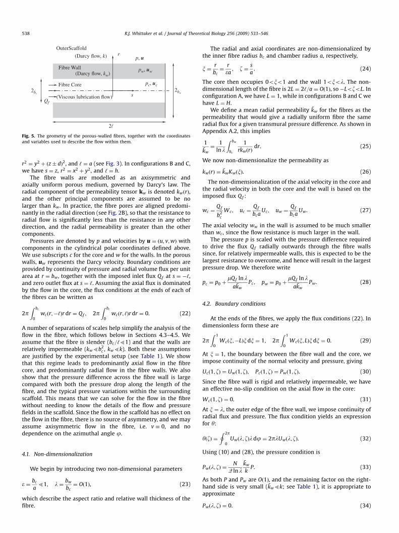
The porous fibres are modelled as circular cylinders of length2‘ and external diameter 2bw, with a hollow core of internaldiameter 2bc. See Fig. 5. We use cylindrical polar coordinatesðr;j; sÞ aligned with the fibre. In configuration A, we have s ¼ x,
ARTICLE IN PRESS
Fig. 5. The geometry of the porous-walled fibres, together with the coordinates
and variables used to describe the flow within them.
R.J. Whittaker et al. / Journal of Theoretical Biology 256 (2009) 533–546538
r2 ¼ y2 þ ðz dÞ2, and ‘ ¼ a (see Fig. 3). In configurations B and C,we have s ¼ z, r2 ¼ x2 þ y2, and ‘ ¼ h.
The fibre walls are modelled as an axisymmetric andaxially uniform porous medium, governed by Darcy’s law. Theradial component of the permeability tensor kw is denoted kwðrÞ,and the other principal components are assumed to be nolarger than kw. In practice, the fibre pores are aligned predomi-nantly in the radial direction (see Fig. 2B), so that the resistance toradial flow is significantly less than the resistance in any otherdirection, and the radial permeability is greater than the othercomponents.
Pressures are denoted by p and velocities by u ¼ ðu; v;wÞ withcomponents in the cylindrical polar coordinates defined above.We use subscripts c for the core and w for the walls. In the porouswalls, uw represents the Darcy velocity. Boundary conditions areprovided by continuity of pressure and radial volume flux per unitarea at r ¼ bw, together with the imposed inlet flux Qf at s ¼ �‘,and zero outlet flux at s ¼ ‘. Assuming the axial flux is dominatedby the flow in the core, the flux conditions at the ends of each ofthe fibres can be written as
2pZ bc
0wcðr;�‘Þr dr ¼ Qf ; 2p
Z bc
0wcðr; ‘Þr dr ¼ 0. (22)
A number of separations of scales help simplify the analysis of theflow in the fibre, which follows below in Sections 4.3–4.5. Weassume that the fibre is slender (bc=‘51) and that the walls arerelatively impermeable (kw5b2
c , kw5k). Both these assumptionsare justified by the experimental setup (see Table 1). We showthat this regime leads to predominantly axial flow in the fibrecore, and predominantly radial flow in the fibre walls. We alsoshow that the pressure difference across the fibre wall is largecompared with both the pressure drop along the length of thefibre, and the typical pressure variations within the surroundingscaffold. This means that we can solve for the flow in the fibrewithout needing to know the details of the flow and pressurefields in the scaffold. Since the flow in the scaffold has no effect onthe flow in the fibre, there is no source of asymmetry, and we mayassume axisymmetric flow in the fibre, i.e. v 0, and nodependence on the azimuthal angle j.
4.1. Non-dimensionalization
We begin by introducing two non-dimensional parameters
� ¼bc
a51; l ¼
bw
bc¼ Oð1Þ, (23)
which describe the aspect ratio and relative wall thickness of thefibre.
The radial and axial coordinates are non-dimensionalized bythe inner fibre radius bc and chamber radius a, respectively,
x ¼r
bc¼
r
�a; z ¼
s
a. (24)
The core then occupies 0oxo1 and the wall 1oxol. The non-dimensional length of the fibre is 2L ¼ 2‘=a ¼ Oð1Þ, so �LozoL. Inconfiguration A, we have L ¼ 1, while in configurations B and C wehave L ¼ H.
We define a mean radial permeability kw for the fibres as thepermeability that would give a radially uniform fibre the sameradial flux for a given transmural pressure difference. As shown inAppendix A.2, this implies
1
kw
¼1
lnl
Z bw
bc
1
rkwðrÞdr. (25)
We now non-dimensionalize the permeability as
kwðrÞ ¼ kwKwðxÞ. (26)
The non-dimensionalization of the axial velocity in the core andthe radial velocity in both the core and the wall is based on theimposed flux Qf :
wc ¼Qf
b2c
Wc; uc ¼Qf
bcaUc ; uw ¼
Qf
bcaUw. (27)
The axial velocity ww in the wall is assumed to be much smallerthan wc , since the flow resistance is much larger in the wall.
The pressure p is scaled with the pressure difference requiredto drive the flux Qf radially outwards through the fibre wallssince, for relatively impermeable walls, this is expected to be thelargest resistance to overcome, and hence will result in the largestpressure drop. We therefore write
pc ¼ p0 þmQf ln l
akw
Pc ; pw ¼ p0 þmQf ln l
akw
Pw. (28)
4.2. Boundary conditions
At the ends of the fibres, we apply the flux conditions (22). Indimensionless form these are
2pZ 1
0Wcðx;�LÞxdx ¼ 1; 2p
Z 1
0Wcðx; LÞxdx ¼ 0. (29)
At x ¼ 1, the boundary between the fibre wall and the core, weimpose continuity of the normal velocity and pressure, giving
Ucð1; zÞ ¼ Uwð1; zÞ; Pcð1; zÞ ¼ Pwð1; zÞ. (30)
Since the fibre wall is rigid and relatively impermeable, we havean effective no-slip condition on the axial flow in the core:
Wcð1; zÞ ¼ 0. (31)
At x ¼ l, the outer edge of the fibre wall, we impose continuity ofradial flux and pressure. The flux condition yields an expressionfor y:
yðzÞ ¼I 2p
0Uwðl; zÞldj ¼ 2plUwðl; zÞ. (32)
Using (10) and (28), the pressure condition is
Pwðl; zÞ ¼N
Q ln lkw
kP. (33)
As both P and Pw are Oð1Þ, and the remaining factor on the right-hand side is very small (kw5k; see Table 1), it is appropriate toapproximate
Pwðl; zÞ ¼ 0. (34)
ARTICLE IN PRESS
R.J. Whittaker et al. / Journal of Theoretical Biology 256 (2009) 533–546 539
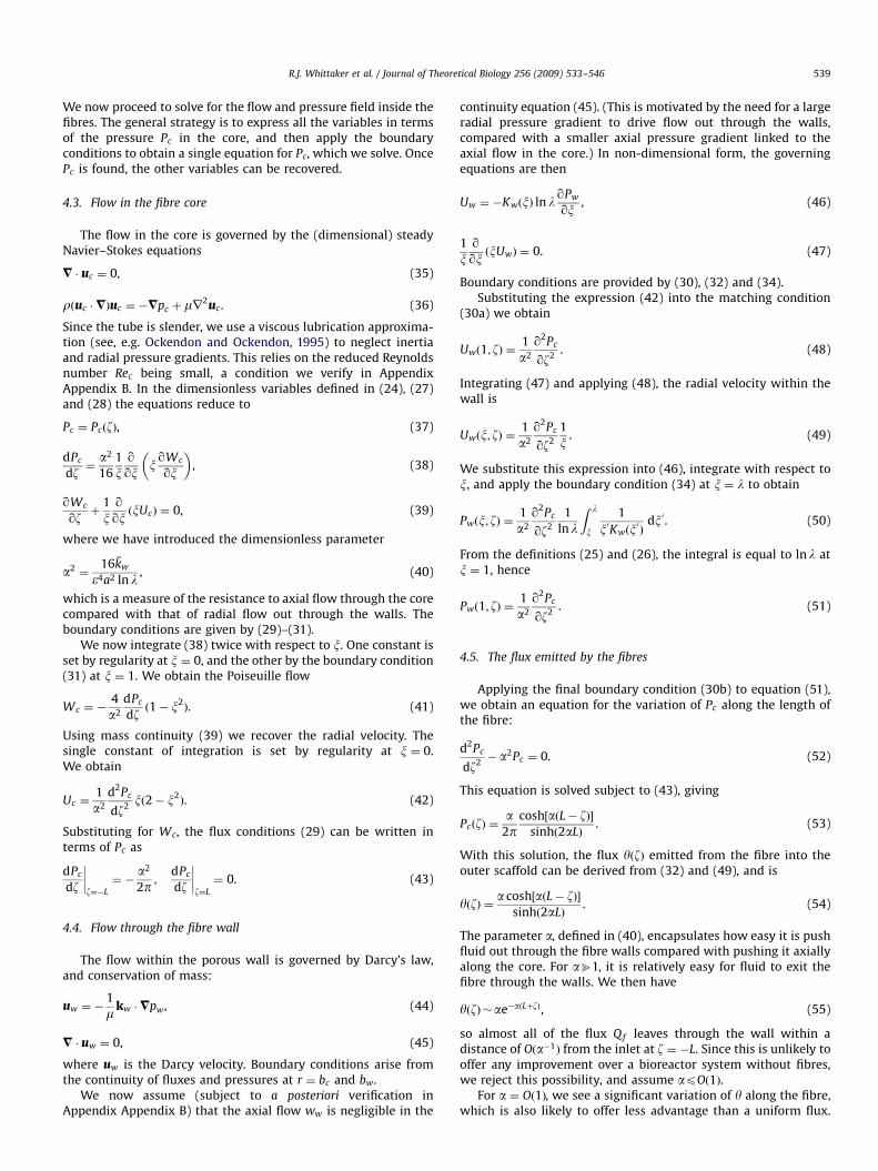
We now proceed to solve for the flow and pressure field inside thefibres. The general strategy is to express all the variables in termsof the pressure Pc in the core, and then apply the boundaryconditions to obtain a single equation for Pc, which we solve. OncePc is found, the other variables can be recovered.
4.3. Flow in the fibre core
The flow in the core is governed by the (dimensional) steadyNavier–Stokes equations
= � uc ¼ 0, (35)
rðuc �=Þuc ¼ �=pc þ mr2uc . (36)
Since the tube is slender, we use a viscous lubrication approxima-tion (see, e.g. Ockendon and Ockendon, 1995) to neglect inertiaand radial pressure gradients. This relies on the reduced Reynoldsnumber Rec being small, a condition we verify in AppendixAppendix B. In the dimensionless variables defined in (24), (27)and (28) the equations reduce to
Pc ¼ PcðzÞ, (37)
dPc
dz¼a2
16
1
xqqx
xqWc
qx
� �, (38)
qWc
qzþ
1
xqqxðxUcÞ ¼ 0, (39)
where we have introduced the dimensionless parameter
a2 ¼16kw
�4a2 ln l, (40)
which is a measure of the resistance to axial flow through the corecompared with that of radial flow out through the walls. Theboundary conditions are given by (29)–(31).
We now integrate (38) twice with respect to x. One constant isset by regularity at x ¼ 0, and the other by the boundary condition(31) at x ¼ 1. We obtain the Poiseuille flow
Wc ¼ �4
a2
dPc
dzð1� x2
Þ. (41)
Using mass continuity (39) we recover the radial velocity. Thesingle constant of integration is set by regularity at x ¼ 0.We obtain
Uc ¼1
a2
d2Pc
dz2xð2� x2
Þ. (42)
Substituting for Wc, the flux conditions (29) can be written interms of Pc as
dPc
dz
����z¼�L
¼ �a2
2p ;dPc
dz
����z¼L
¼ 0. (43)
4.4. Flow through the fibre wall
The flow within the porous wall is governed by Darcy’s law,and conservation of mass:
uw ¼ �1
mkw �=pw, (44)
= � uw ¼ 0, (45)
where uw is the Darcy velocity. Boundary conditions arise fromthe continuity of fluxes and pressures at r ¼ bc and bw.
We now assume (subject to a posteriori verification inAppendix Appendix B) that the axial flow ww is negligible in the
continuity equation (45). (This is motivated by the need for a largeradial pressure gradient to drive flow out through the walls,compared with a smaller axial pressure gradient linked to theaxial flow in the core.) In non-dimensional form, the governingequations are then
Uw ¼ �KwðxÞ ln lqPw
qx, (46)
1
xqqxðxUwÞ ¼ 0. (47)
Boundary conditions are provided by (30), (32) and (34).Substituting the expression (42) into the matching condition
(30a) we obtain
Uwð1; zÞ ¼1
a2
q2Pc
qz2. (48)
Integrating (47) and applying (48), the radial velocity within thewall is
Uwðx; zÞ ¼1
a2
q2Pc
qz2
1
x. (49)
We substitute this expression into (46), integrate with respect tox, and apply the boundary condition (34) at x ¼ l to obtain
Pwðx; zÞ ¼1
a2
q2Pc
qz2
1
ln l
Z l
x
1
x0Kwðx0Þ
dx0. (50)
From the definitions (25) and (26), the integral is equal to lnl atx ¼ 1, hence
Pwð1; zÞ ¼1
a2
q2Pc
qz2. (51)
4.5. The flux emitted by the fibres
Applying the final boundary condition (30b) to equation (51),we obtain an equation for the variation of Pc along the length ofthe fibre:
d2Pc
dz2� a2Pc ¼ 0. (52)
This equation is solved subject to (43), giving
PcðzÞ ¼a
2pcosh½aðL� zÞ�
sinhð2aLÞ. (53)
With this solution, the flux yðzÞ emitted from the fibre into theouter scaffold can be derived from (32) and (49), and is
yðzÞ ¼a cosh½aðL� zÞ�
sinhð2aLÞ. (54)
The parameter a, defined in (40), encapsulates how easy it is pushfluid out through the fibre walls compared with pushing it axiallyalong the core. For ab1, it is relatively easy for fluid to exit thefibre through the walls. We then have
yðzÞ�ae�aðLþzÞ, (55)
so almost all of the flux Qf leaves through the wall within adistance of Oða�1Þ from the inlet at z ¼ �L. Since this is unlikely tooffer any improvement over a bioreactor system without fibres,we reject this possibility, and assume apOð1Þ.
For a ¼ Oð1Þ, we see a significant variation of y along the fibre,which is also likely to offer less advantage than a uniform flux.

ARTICLE IN PRESS
Z
Y
−0.8 −0.6 −0.4 −0.2 0 0.2 0.4 0.6 0.8
−0.6
−0.4
−0.2
0
0.2
0.4
0.6
0
0.2
0.4
0.6
0.8
1
1.2
1.4
1.6
1.8
2
|V |
Fig. 8. The magnitude of the dimensionless Darcy velocity in the plane X ¼ 0:3 in
configuration A with Q ¼ 0:4. Other details as in Fig. 6. Flow is generally from left
R.J. Whittaker et al. / Journal of Theoretical Biology 256 (2009) 533–546540
At the other extreme, a51, we have
yðzÞ�1
2L(56)
so the emitted flux is uniform along the length of the fibre.
4.6. Summary
We have found the solution for the flow in the fibres. Thepressure Pc in the core is given by (53) and this can be substitutedback into the previous expressions for the other physical variables.The dimensionless flux per unit length y emitted at each pointalong the length of the fibre is given by (54). This expression cannow be used to complete the model for the flow in the scaffolddeveloped in Section 3. In Appendix B, we confirm that the variousapproximations we have used are valid for the experimental setupbeing modelled.
Table 2Typical values of the various dimensionless parameters appearing in Sections 2–4,
computed from the values in Table 1.
H � l k=a2 kw=b2c
a2
0:7 0:02 3 10�4 10�6 0:07
Z
Y
−0.8 −0.6 −0.4 −0.2 0 0.2 0.4 0.6 0.8
−0.6
−0.4
−0.2
0
0.2
0.4
0.6
0
0.2
0.4
0.6
0.8
1
1.2
1.4
1.6
1.8
2
|V |
Fig. 6. The magnitude of the dimensionless Darcy velocity V in the vertical plane
X ¼ 0:3 in configuration A with Q ¼ 0 (i.e. no flux from the fibres). The inlet is out
of the plane to the left, and the outlet lies similarly to the right. The two fibres run
perpendicular to the plane through Y ¼ 0, Z ¼ 0:35. From the dimensionless
Darcy velocity, the dimensional equivalent can be recovered from (10), and an
estimate for the shear stress found using (58).
Z
Y
−0.8 −0.6 −0.4 −0.2 0 0.2 0.4 0.6 0.8
−0.6
−0.4
−0.2
0
0.2
0.4
0.6
0
0.2
0.4
0.6
0.8
1
1.2
1.4
1.6
1.8
2
|V |
Fig. 7. The magnitude of the dimensionless Darcy velocity in the plane X ¼ 0:3 in
configuration A with Q ¼ 0:2. Other details as in Fig. 6. Flow is generally from left
to right, and fluid is emitted by the fibres.
to right, and fluid is emitted by the fibres.
5. Numerical solutions for the fluid flow
In all the numerical computations, we take a51 so that (56)holds and the flux emitted by the fibres is uniform along theirlength. A uniform flux is desirable from a theoretical standpoint,as it is likely to result in a more even distribution of culturemedium flow and shear stresses. Furthermore, for the fibres beingconsidered for use in the prototype bioreactors that motivated thisstudy, we have a ¼ Oð10�1
Þ51 (see (40) and Table 2).With yðzÞ given by (56), the model developed in Section 3 then
leads to the problem of solving Poisson’s equation (12) for thepressure P in the cylindrical bioreactor chamber. We haveDirichlet and/or Neumann boundary conditions on the walls,and a number of delta-function source terms representing thefibres and inlet/outlet pipes. The equations and boundaryconditions for the three fibre configurations considered in thispaper are given in Section 3.2.
Similar systems of equations arise in many physical problems,and solution techniques are well-developed. We solved thesystem numerically using the Electrostatics package of the‘COMSOL Multiphysics’ computer program,3 which uses a finiteelement technique. Once the pressure P has been computed, theDarcy velocity V is determined from (11).
For each of the three configurations, the flow may be solvedwith typical parameter values to provide insight into how thefibres affect the flow. In all cases, we used an aspect ratio ofH ¼ 0:7, in line with the experimental prototype shown in Fig. 1.The graphs show the magnitude jV j of the Darcy velocity on aplanar cross-section through the bioreactor chamber.
For configuration A, we used a fibre separation 2D ¼ 0:7 (seeFig. 3). Results are shown on an off-centre vertical planeperpendicular to the fibres at X ¼ 0:3. We consider a fixed totalflux Q� with three different values of the proportion Q from thefibres: 0, 0:2, and 0:4. The results are shown in Figs. 6–8. Otherparallel planes show essentially the same qualitative structure,with a dipole structure around the fibres and larger velocities inthe vicinity of the inlet and outlet pipes. The off-centre planeswere chosen to avoid the singularities at these points.
For configurations B and C, there is a single vertical fibre, andwe use off-centre horizontal cross-sections at Z ¼ 0:3 instead. Forconfiguration B, we again present results for Q ¼ 0;0:2;0:4. SeeFigs. 9–11. For configuration C, there are no separate input flows so
3 Developed and distributed by COMSOL Inc. Full details available online at
http://www.comsol.com/.

ARTICLE IN PRESS
X
Y
−0.8 −0.6 −0.4 −0.2 0 0.2 0.4 0.6 0.8
−0.8
−0.6
−0.4
−0.2
0
0.2
0.4
0.6
0.8
0
0.2
0.4
0.6
0.8
1
1.2
1.4
1.6
1.8
2
|V|
Fig. 11. The magnitude of the Darcy velocity in the plane Z ¼ 0:3 in configuration B
with Q ¼ 0:4. Other details as in Fig. 9. Flow is generally from left to right, with
fluid emitted by the fibre.
X
Y
−0.8 −0.6 −0.4 −0.2 0 0.2 0.4 0.6 0.8
−0.8
−0.6
−0.4
−0.2
0
0.2
0.4
0.6
0.8
0
0.2
0.4
0.6
0.8
1
1.2
1.4
1.6
1.8
2
|V |
Fig. 10. The magnitude of the Darcy velocity in the plane Z ¼ 0:3 in configuration B
with Q ¼ 0:2. Other details as in Fig. 9. Flow is generally from left to right, with
fluid emitted by the fibre.
X
Y
−0.8 −0.6 −0.4 −0.2 0 0.2 0.4 0.6 0.8
−0.8
−0.6
−0.4
−0.2
0
0.2
0.4
0.6
0.8
0
0.2
0.4
0.6
0.8
1
1.2
1.4
1.6
1.8
2
|V |
Fig. 12. The magnitude of the Darcy velocity in any horizontal plane Z ¼ Z0 in
configuration C. Other details as in Fig. 9. Flow is radially outwards from the
central fibre source.
X
Y
−0.8 −0.6 −0.4 −0.2 0 0.2 0.4 0.6 0.8
−0.8
−0.6
−0.4
−0.2
0
0.2
0.4
0.6
0.8
0
0.2
0.4
0.6
0.8
1
1.2
1.4
1.6
1.8
2
|V |
Fig. 9. The magnitude of the dimensionless Darcy velocity V in the plane Z ¼ 0:3
in configuration B with Q ¼ 0 (no flow from the fibre). The single fibre runs
perpendicular to the plane, through X ¼ Y ¼ 0. The inlet pipe is to the left and the
outlet pipe to the right, both in the plane Z ¼ 0. From the dimensionless Darcy
velocity, the dimensional equivalent can be recovered from (10), and an estimate
for the shear stress found using (58).
R.J. Whittaker et al. / Journal of Theoretical Biology 256 (2009) 533–546 541
Q 1. The solution, which can be obtained analytically, is ofpurely radial flow, and is shown in Fig. 12.
The computations show that without the fibres (Q ¼ 0), flowrates are highest in the vicinity of the inlet and outlet pipes, aswould be expected. The slowest regions of the flow are found nearthe chamber walls on the plane Y ¼ 0. The addition of the fibresincreases relative flow rates on the downstream side of them(Y40), but also decreases the flow on the upstream side (Yo0).These increases and decreases become more pronounced as Qincreases.
6. Shear stress
As discussed in the Introduction, bone cells are sensitive to fluidshear stresses. Some shear stress is necessary for viable growth, buthigher levels may damage the cells. It is therefore important to
calculate the shear-stress distribution associated with the flowfields computed in Section 5. The shear stresses will be propor-tional to the overall flow rate Q�, which therefore needs to beadjusted so as to provide sufficient shear (and nutrient delivery)over as much of the scaffold as possible, while constrainingexcessively high shear to as small a region as possible.
The shear stress experienced by the cells within the individualscaffold pores can be estimated from the Darcy velocity as follows.We first take the estimate U�jvjt=f for the mean magnitude ofthe interstitial velocity. We then use Poiseuille flow of meanvelocity U through a circular duct of diameter d as anapproximate model for the local flow within each scaffold pore.With r as a local radial coordinate, the velocity profile is
v � 2U 1�2r
d
� �2" #
(57)

ARTICLE IN PRESS
Table 3Typical values of the experimental parameters related to the nutrient problem.
Parameter Symbol Typical value
Time scale for fluid circulation tc 3:4� 100 s
Time scale for cell growth t1=2 2� 105 s
Time scale for culturing tg 6� 105–3� 106 s
Initial number of cells per unit volume n0 1� 1012 cells m�3
All values based on the experimental setup of Cartmell and Michael, apart from tc which is calculated using (65). For other properties, see Table 1.
Table 4Typical properties relating to two nutrients and a waste product that are relevant to the cells.
Nutrient or product c�i ( mol m�3) cyi ( mol m�3) ki ( m2 s�1) si ( mol cell�1 s�1) tdi ( s)
Glucose 5:6 0 7� 10�10�8� 10�17 4:3� 102
Oxygen (O2) 1:0 0 3� 10�9�4:2� 10�17 1:5� 102
Lactic acid 0 0:4 1� 10�9 1:4� 10�16 1:8� 101
The initial concentration c�i in the culture medium as it enters the bioreactor, the concentration cyi that would be detrimental to the cells, the diffusivity ki and the rate of
production si (negative in the case of uptake). Glucose concentration from culture medium product data (Invitrogen, 2008), and initial oxygen concentration based on
solubility in water at 37 �C and 1 atm (Tromans, 1998). Approximate diffusivities for dilute solutions at 25–30 �C from Lide (2007), with the exception of lactic acid from
Ribeiro et al. (2005). Typical uptake and production rates inferred from Komarova et al. (2000). The estimate for cyi for lactic acid is discussed in Appendix A.3. Depletion/
accumulation times tdi calculated using (66), assuming n ¼ nmax ¼ 1:3� 1014 and f ¼ 0:8.
R.J. Whittaker et al. / Journal of Theoretical Biology 256 (2009) 533–546542
and the wall shear stress is
S ¼ m qv
qr
��������ðr¼d=2Þ
�8mUd�
8mtfdjvj ¼
8mQ�tfda2
jV j. (58)
The first two approximations for S use the velocity profile (57) andthe estimate for U above; the final equality comes from the non-dimensionalization (10). While obviously not precise, (58) gives areasonable estimate (at least in order-of-magnitude terms) for theshear stress experienced by the cells in terms of the local Darcyvelocity and the fluid and scaffold properties. For the values givenin Table 1 we obtain
S ¼Q�
4:8� 10�6 m3 s�1
� �jV jPa. (59)
From the numerical results, jV j ¼ Oð1Þ over most of the chamber,and exceeds 2 only in small regions near the fibres and inlet/outletpipes. Thus, to obtain shear stresses of the order of Pascals (as inthe experiments referenced in the Introduction), volume fluxes ofthe order of 10�5–10�6 m3 s�1 need to be used. This is somewhathigher than the anticipated value Q��10�7 m3 s�1 in Table 1.
However, in any particular experiment, the desirable volumeflux will depend on the requirements of the cells and on the exactproperties of the bioreactor system being used. It may also beconstrained by the availability of pumping equipment and thepressures required to force fluid through the system. We thereforeleave the results in general terms, rather than trying to makedefinite predictions that may not apply in other situations.Another factor to consider is the effect of the flow rate uponnutrient and waste transport. This issue is addressed in thefollowing section.
4 Note that this is number of cells per unit total volume of bioreactor chamber,
not the number per unit volume of pore space.
7. Nutrient and waste transport
One of the most important requirements for both survival andproliferation of the cells is the supply of nutrients and the removalof waste products. In the case of nutrients the supply must besufficient to meet the demands of the proliferating cells, while inthe case of waste products we need to ensure they are removedsufficiently rapidly to prevent any build-up that would be
harmful. For example a build-up of lactic acid could cause aharmful change in pH (see A.3).
We use simple scaling arguments here to determine whetheror not nutrient depletion or waste-product accumulation aresignificant effects over the relevant time scales in the culturingprocess. Key conclusions can be drawn without the need to solvethe full system of equations explicitly.
Suppose that the cells are initially seeded on to the scaffoldwith a density n0 per unit volume4 and then proliferate over theculturing period. We assume a constant doubling time of t1=2, sothat the number of cells per unit volume at time t after the start ofculturing is
n ¼ n0 expt ln 2
t1=2
� �. (60)
The maximum cell density nmax is achieved when t ¼ tg atthe end of the culturing period. Typical values of n0, t1=2
and tg , given in Table 3, indicate that the cells may double innumber around 7 times over the culturing period tg , leading tonmax � 1:3� 1014 m�3.
The concentration ci of an individual nutrient or waste producti in the fluid occupying the pore space of the scaffold is governedby an advection–diffusion equation
qci
qtþ u �=ci ¼ kir
2ci, (61)
where ki is the diffusivity of species i (assumed to be constantover the range of concentrations considered) and uðxÞ is thevelocity of the fluid. Boundary conditions arise from theconcentration in the culture medium at the inlets, and a fluxcondition describing uptake or production at the cell surfaces.
A simple averaged model describes each concentration field asa local average ci (taken over the pore spaces), and includes theuptake or production by the cells as a source term. Following
ARTICLE IN PRESS
R.J. Whittaker et al. / Journal of Theoretical Biology 256 (2009) 533–546 543
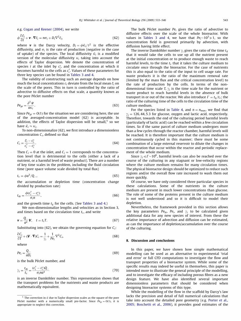
e.g. Cogan and Keener (2004), we write
fqci
qtþ v �=ci ¼ nsi þ Dir
2ci, (62)
where v is the Darcy velocity, Di ¼ fki=t2 is the effectivediffusivity, and si is the rate of production (negative in the caseof uptake) of the species. The local diffusivity ki is a modifiedversion of the molecular diffusivity ki taking into account theeffects of Taylor dispersion. We denote the concentration ofspecies i at the inlet by c�i , and the concentration at which itbecomes harmful to the cells as cyi . Values of these parameters forthree key species can be found in Tables 3 and 4.
The validity of constructing such an average depends on howmuch the local concentrations ci deviate from the local mean ci onthe scale of the pores. This in turn is controlled by the ratio ofadvective to diffusive effects on that scale, a quantity known asthe pore Peclet number
Pepi ¼d2U
aki. (63)
Since Pepi ¼ Oð1Þ for the situation we are considering here, the useof the averaged-concentration model (62) is acceptable. Inaddition, the effects of Taylor dispersion will be small,5 so wehave ki � ki.
To non-dimensionalize (62), we first introduce a dimensionlessconcentration Ci, defined so that
Ci ¼ci � c�icyi � c�i
. (64)
Then Ci ¼ 0 at the inlet, and Ci ¼ 1 corresponds to the concentra-tion level that is detrimental to the cells (either a lack of anutrient, or a harmful level of waste product). There are a numberof key time scales in the problem, including the fluid circulationtime (pore space volume scale divided by total flux)
tc ¼ fa3=Q�, (65)
the accumulation or depletion time (concentration changedivided by production rate)
tdi ¼fðcyi � c�i Þ
sin, (66)
and the growth time tg for the cells. (See Tables 3 and 4.)We non-dimensionalize lengths and velocities as in Section 3,
and times based on the circulation time tc, and write
v ¼Q�a2
V ; t ¼ tcT . (67)
Substituting into (62), we obtain the governing equation for Ci:
qCi
qTþ ðV �=ÞCi ¼
1
gi
þ1
Peir2Ci, (68)
where
Pei ¼Q�aDi
(69)
is the bulk Peclet number, and
gi ¼tdi
tc¼ðcyi � c�i ÞQ�
sina3(70)
is an inverse Damkohler number. This representation shows thatthe transport problems for the nutrients and waste products aremathematically equivalent.
5 The correction in k due to Taylor dispersion scales as the square of the pore
Peclet number with a numerically small pre-factor. Since Pepi ¼ Oð1Þ, it is
appropriate to neglect this correction.
The bulk Peclet number Pei gives the ratio of advective todiffusive effects over the scale of the whole bioreactor. Withvalues in Tables 3 and 4, we have that Pei�103
b1, so theconcentration field is governed primarily by advection, withdiffusion having little effect.
The inverse Damkohler number gi gives the ratio of the time td
that it would take the cells to use up all the nutrient presentat the initial concentration or to produce enough waste to reachharmful levels, to the time tc that it takes the culture medium tocirculate once through the bioreactor. For the case of nutrientsthis is also equal to the ratio of the input to cell usage rate. Forwaste products it is the ratio of the maximum removal rate(limited by the mass flux and the critical concentration level) tothe rate of production by the cells. In terms of the non-dimensional time scale T, gi is the time scale for the nutrient orwaste product to reach harmful levels in the absence of bulktransport in or out of the reactor. We also introduce G ¼ tg=tc; theratio of the culturing time of the cells to the circulation time of theculture medium.
For the species listed in Table 4, and n ¼ nmax, we find thatgi ¼ 126;44;5:3 for glucose, oxygen and lactic acid, respectively.Therefore, towards the end of the culturing period harmful levels(particularly of lactic acid) can be reached within a few circulationtimes. So if the same parcel of culture medium undergoes morethan a few cycles through the reactor chamber, harmful levels willbe reached. It is therefore important that the culture medium isnot continuously cycled in this manner; there must be somecombination of a large external reservoir to dilute the changes inconcentration that occur within the reactor and periodic replace-ment of the whole medium.
Since gi5G�106, harmful levels can also be reached over thecourse of the culturing in any stagnant or low-velocity regionswhere the culture medium remains for many circulation times.The physical bioreactor design should be optimized to reduce suchregions and/or the overall flow rate increased to wash them outmore quickly.
Of course, we have only considered three particular species inthese calculations. Some of the nutrients in the culturemedium are present in much lower concentrations than glucose.The role of some of the proteins present in the culture mediumis not well understood and so it is difficult to model theirdepletion.
Nevertheless, the framework provided in this section allowsthe key parameters Pebi, Pei, and gi to be calculated givenadditional data for any new species of interest. From these therelative importance of advection and diffusion can be estimated,as can the importance of depletion/accumulation over the courseof the culturing.
8. Discussion and conclusions
In this paper, we have shown how simple mathematicalmodelling can be used as an alternative to experimental ‘trialand error’ or full CFD computations to investigate the flow andtransport properties of a bioreactor system. While some of thespecific results may indeed be useful in themselves, this paper isintended more to illustrate the general principle of the modelling,and to investigate the efficacy of including porous fibres as a newdesign feature. We have also identified several importantdimensionless parameters that should be considered whendesigning bioreactor systems of this type.
While the modelling of the flow in the scaffold by Darcy’s lawlacks the precision and detail of full numerical calculations thattake into account the detailed pore geometry (e.g. Porter et al.,2005; Boschetti et al., 2006), it provides good estimates of the
ARTICLE IN PRESS
R.J. Whittaker et al. / Journal of Theoretical Biology 256 (2009) 533–546544
global flow field, shear stresses, and nutrient transport within thescaffold. The advantages of this approach are the Darcy model’ssimplicity, the ease and rapidity of obtaining results for manydifferent scenarios, and the fact that by averaging the scaffoldgeometry, we do not require the detailed pore geometry,information that is expensive to obtain and, moreover, changesfrom one scaffold to another.
In terms of the shear stresses and nutrient transport withinthe bioreactor, we have shown how these may be estimatedfrom the properties of the system under consideration. Inparticular, the theoretical approach can be used to guide thedesign of future systems. Using our framework, experimentalistscan estimate in advance the range of flow rates required toachieve a desired shear-stress distribution and ensure sufficientnutrient and waste-product transport. They can also determinehow often the culture medium may need to be replenished duringthe culturing.
Returning to the particular cases studied here, the resultsshown in Figs. 9–11 for configurations A and B suggest that addingfibres perpendicular to the main flow from the inlet and outletpipes will probably not result in a beneficial change to the flowdistribution. While there is an increase in the flow rates on thedownstream side of the fibres, there is a corresponding decreaseon the upstream side. However, perhaps oscillating the inlet/outlet or fibre flows may be able to counteract this. Nevertheless,the presence of the fibres can do little to increase flow rates in thestagnant corner regions, which are arguably the areas in need ofmost help.
The final configuration C fares much better. Using the fibre asthe only source of fluid, and having a distributed outlet, ensures amore uniformly distributed flow. However, since the radial flux(radial velocity times 2pr) is constant, higher velocities, and henceshear rates, are experienced near the axis. Depending on theprecise sensitivity of the cells to the applied shear stress, this mayor may not be problematic.
With regard to the fibres themselves, we have identifieda key dimensionless parameter a, defined in (40), which is afunction of the material properties and dimensions of thefibre. As discussed in Section 4.5, the value of a describes therelative ease of flow through the fibre walls compared withflow through the hollow fibre core. An outflow through thewalls that is uniform along the length of the fibre is obtained ifand only if a51. Since we are interested in obtaining auniform distribution of flow, this is the only regime we haveconsidered in detail here. Knowledge of the pressures required toforce a particular flow-rate through a particular fibre shouldprove useful in guiding the choice of fibre properties and pumpsetup.
Acknowledgements
This paper came about as an extension to a problem (Baileyet al., 2006) considered at the 6th Mathematics in Medicine StudyGroup, held at the University of Nottingham in September 2006,with funding from the Engineering and Physical Sciences ResearchCouncil (EPSRC).
The authors would also like to specifically acknowledge JonGittings and Irene Turner who manufacture the scaffolds (seeGittings et al., 2005) for the project that motivated this study.
Dr. Cartmell and Dr. Kuiper wish to acknowledge the financialsupport of a private local charity. Dr Waters is grateful to theEPSRC for funding in the form of an Advanced Research Fellow-ship. Dr. Cummings wishes to thank the City College of New York’sDepartment of Chemical Engineering and Levich Institute forhospitality during a stay as a visiting professor.
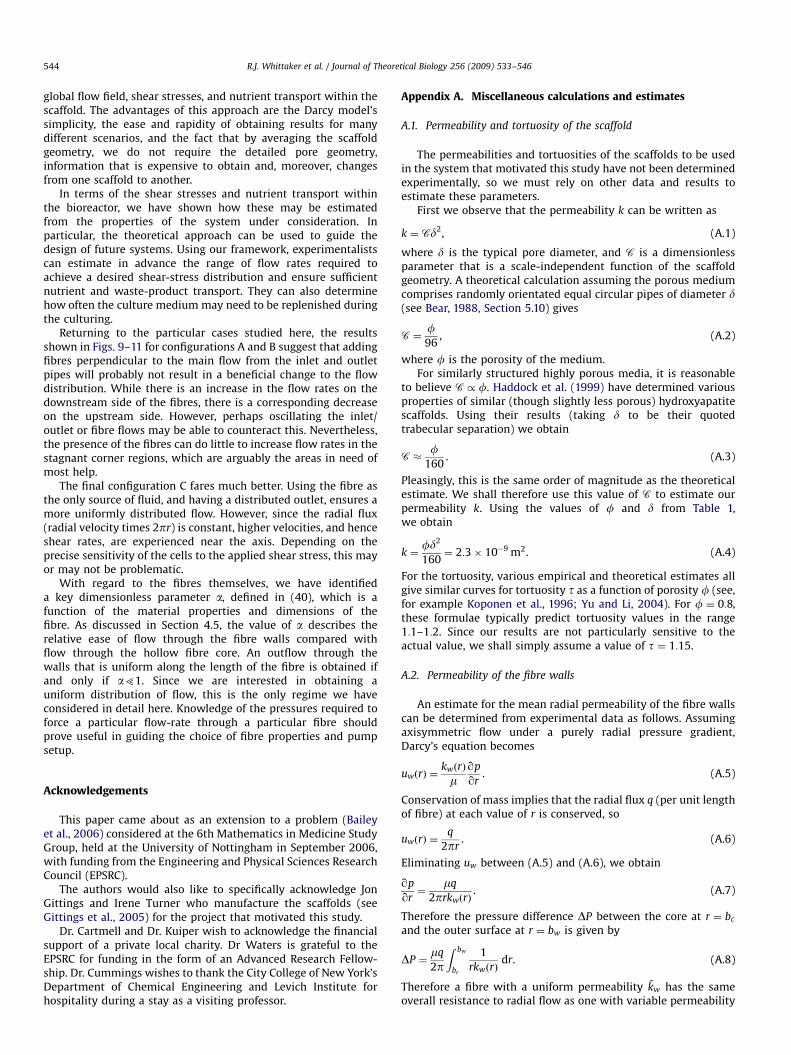
Appendix A. Miscellaneous calculations and estimates
A.1. Permeability and tortuosity of the scaffold
The permeabilities and tortuosities of the scaffolds to be usedin the system that motivated this study have not been determinedexperimentally, so we must rely on other data and results toestimate these parameters.
First we observe that the permeability k can be written as
k ¼ Cd2, (A.1)
where d is the typical pore diameter, and C is a dimensionlessparameter that is a scale-independent function of the scaffoldgeometry. A theoretical calculation assuming the porous mediumcomprises randomly orientated equal circular pipes of diameter d(see Bear, 1988, Section 5.10) gives
C ¼f96
, (A.2)
where f is the porosity of the medium.For similarly structured highly porous media, it is reasonable
to believe C / f. Haddock et al. (1999) have determined variousproperties of similar (though slightly less porous) hydroxyapatitescaffolds. Using their results (taking d to be their quotedtrabecular separation) we obtain
C �f
160. (A.3)
Pleasingly, this is the same order of magnitude as the theoreticalestimate. We shall therefore use this value of C to estimate ourpermeability k. Using the values of f and d from Table 1,we obtain
k ¼fd2
160¼ 2:3� 10�9 m2. (A.4)
For the tortuosity, various empirical and theoretical estimates allgive similar curves for tortuosity t as a function of porosity f (see,for example Koponen et al., 1996; Yu and Li, 2004). For f ¼ 0:8,these formulae typically predict tortuosity values in the range1:1–1:2. Since our results are not particularly sensitive to theactual value, we shall simply assume a value of t ¼ 1:15.
A.2. Permeability of the fibre walls
An estimate for the mean radial permeability of the fibre wallscan be determined from experimental data as follows. Assumingaxisymmetric flow under a purely radial pressure gradient,Darcy’s equation becomes
uwðrÞ ¼kwðrÞ
mqp
qr. (A.5)
Conservation of mass implies that the radial flux q (per unit lengthof fibre) at each value of r is conserved, so
uwðrÞ ¼q
2pr. (A.6)
Eliminating uw between (A.5) and (A.6), we obtain
qp
qr¼
mq
2prkwðrÞ. (A.7)
Therefore the pressure difference DP between the core at r ¼ bc
and the outer surface at r ¼ bw is given by
DP ¼mq
2p
Z bw
bc
1
rkwðrÞdr. (A.8)
Therefore a fibre with a uniform permeability kw has the sameoverall resistance to radial flow as one with variable permeability

ARTICLE IN PRESS
6.5
7
7.5
8
0
pH
Concentration of Lactic Acid (mol m−3)
0.2 0.4 0.6 0.8 1 1.2 1.4
Fig. A1. The results of two titrations lactic acid into a typical culture medium to
assess the level of buffering present. The culture medium comprised D-MEM
(Invitrogen, 2008) with 10% fetal calf serum. Lactic acid was added drop-wise
using a pipette, and data points comprising the volume added together with the
pH of the solution were recorded. The agreement between the two titrations
indicates good reproducibility.
R.J. Whittaker et al. / Journal of Theoretical Biology 256 (2009) 533–546 545
kwðrÞ if and only if
Z bw
bc
1
rkw
dr ¼
Z bw
bc
1
rkwðrÞdr, (A.9)
which is the definition for kw used in (25). Using this definition toeliminate kwðrÞ from (A.8), we find that
kw ¼mq
2pDPln
bw
bc
� �. (A.10)
Preliminary experimental data from Ellis and Chaudhuri (unpub-lished) suggests an order of magnitude estimate of kw�10�17 m2,but this figure is likely to be quite sensitive to changes in themanufacturing conditions.
A.3. Harmful concentration of lactic acid
In this appendix, we describe how we estimate the concentra-tion of lactic acid that would be harmful to the growing cells (seeTable 4). When the pH drops the proliferation of cells is stronglyinhibited. Each molecule of glucose produces two molecules oflactic acid and so the rate of production of lactic acid is twice therate of glucose consumption.
The culture medium is initially at a pH of 8, and we assumethat the growing cells can tolerate a pH change of up to 0:5,though growth rates are likely to be affected near to theextremities of this range.
In this pH range, lactic acid is almost fully dissociated and sobehaves as a strong acid. Therefore in the absence of buffering theconcentration of lactic acid required to cause a drop from 8 to 7.5is given by
ð10�7:52 10�8
Þmol dm�3� 2� 10�5 mol m�3. (A.11)
This is a tiny amount relative to the rates at which lactic acid isknown to be produced by the cells, so it is therefore necessary totake the buffering into account.
Culture media typically contain a large number of differentproteins, salts, and other nutrients, which will interact witheach other in complex ways under applied pH changes. Wetherefore make no attempt to model the buffering effect, andinstead appeal to experimental results. Fig. A1 shows data fromtwo titrations of lactic acid into a typical culture medium. Fromthis data, we see that the concentration of lactic acid that resultsin a pH drop of 0.5 is roughly 0:4 mol m�3. We use this for thevalue of cyi in Section 7.
Appendix B. Consistency of the approximations used in Section 4
In this appendix, we check the consistency of the variousapproximations used in Section 4 to model the flow in the fibre.These approximations simplified the equations in the core andwall. We check their validity by comparing the sizes of theneglected terms to those retained.
To obtain the viscous lubrication approximation (37)–(39) inthe fibre core, we assumed that the appropriate Reynolds numberis small, and that the radial pressure variation Dpr required todrive the radial flow is small compared with the axial pressurevariation Dps. The Reynolds number is estimated by comparingthe steady inertia term with the viscous term. We find that
Rec ¼rw2
c =a
mwc=b2c
�rQf
ma¼rQ�ma
Q
N�
20Q
NtOð1Þ. (B.1)
While this may not be formally small, low-Reynolds-numberapproximations are generally found to be acceptable even at Oð1ÞReynolds numbers. Moreover, in the a2
51 regime of primaryinterest here, Oð1Þ errors in the viscous pressure drop along thefibre will not affect the pressure difference across the wall, and sothe emitted flux will be unchanged.
The pressure variations Dpr and Dps are estimated from theviscous drag due to the velocity components. We therefore have
Dps
L�mwc
b2c
�mQf
b4c
;Dpr
bc�m uc
b2c
�mQf
ab3c
, (B.2)
and hence
Dpr
Dps
�b2
c
‘a2� �2. (B.3)
We have already assumed that �51, so the approximation isjustified.
Secondly, when forming equations (46)–(47) for the flow in thewall, we assumed that the axial flow made no contribution to thecontinuity equation, and so could be neglected. Knowing thatthe axial pressure variations in the wall are tied to pcðsÞ from(30b), we can now estimate
qww
qst
kw
mq2pc
qs2�
Qf
a3
q2Pc
qz2�a2Qf
a3�
Qf kw
�4a5. (B.4)
This must be small compared with uw=bc�Qf =ð�2a3Þ. Hence werequire
kw5�2a2 ¼ b2c , (B.5)
a condition that we had already noted.
References
Abousleiman, R.I., Sikavitsas, V.I., 2006. Bioreactors for tissues of the musculoske-letal system. Adv. Exp. Med. Biol. 585, 243–259.
Bailey, C., et al., 2006. Optimisation of fluid distribution inside a porous construct.In: Proceedings of the 6th Mathematics in Medicine Study Group. University ofNottingham.
Bancroft, G., Sikavitsas, V., van den Dolder, J., Sheffield, T., Ambrose, C., Jansen, J.,Mikos, A., 2002. Fluid flow increases mineralized matrix deposition in 3Dperfusion culture of marrow stromal osteoblasts in a dose-dependent manner.Proc. Natl. Acad. Sci. USA 99 (20), 12600–12605.
Batchelor, G.K., 1967. An Introduction to Fluid Dynamics. Cambridge UniversityPress, Cambridge.
Bear, J., 1988. Dynamics of Fluids in Porous Media. Dover.Boschetti, F., Raimondo, M.T., Migliavacca, F., Dubini, G., 2006. Prediction of the
micro-fluid dynamic environment imposed to three-dimensional engineeredcell systems in bioreactors. J. Biomech. 39, 418–425.
Cartmell, S.H., Porter, B.D., Garcia, A.J., Guldberg, R.E., 2003. Effects of mediumperfusion rate on cell-seeded three-dimensional bone constructs in vitro.Tissue Eng. 9 (6), 1197–1203.
Cartmell, S.H., Gittings, J.P., Turner, I.G., Chaudhuri, J.B., Ellis, M.J., Waters, S.L.,Cummings, L.J., Kuiper, N.J., Michael, V., 2007. Bioreactor design for
ARTICLE IN PRESS
R.J. Whittaker et al. / Journal of Theoretical Biology 256 (2009) 533–546546
osteochondral tissue. In: American Society of Bone and Mineral Research, 29thAnnual Meeting Abstracts Supplement. J. Bone Miner. Res. 22S1, S162.
Cimetta, E., Flaibani, M., Mella, M., Serena, E., Boldrin, L., De Coppi, P., Elvassore, N.,2007. Enhancement of viability of muscle precursor cells on 3D scaffold in aperfusion bioreactor. Int. J. Artif. Organs 30 (5), 415–428.
Cogan, N.G., Keener, J.P., 2004. The role of the biofilm matrix in structuraldevelopment. Math. Med. Biol. 21, 147–166.
Cummings, L.J., Waters, S.L., 2007. Tissue growth in a rotating bioreactor. Part II:flow and nutrient transport problems. Math. Med. Biol. 24, 169–208.
Ellis, M.J., Chaudhuri, J.B., 2007. Poly(lactic-co-glycolic acid) hollow fibremembranes for use as a tissue engineering scaffold. Biotech. Bioeng. 96 (1),177–187.
Galban, C.J., Locke, B.R., 1997. Analysis of cell growth in a polymer scaffold using amoving boundary approach. Biotech. Bioeng. 56 (4), 422–432.
Galban, C.J., Locke, B.R., 1999. Effects of spatial variations of cells and nutrient andproduct concentrations coupled with product inhibition on cell growth in apolymer scaffold. Biotech. Bioeng. 64 (6), 633–643.
Gittings, J.P., Turner, I.G., Miles, A.W., 2005. Calcium phosphate open porousscaffold bioceramics. Key Eng. Mat. 284–286, 349–354.
Glowacki, J., Mizuno, S., Greenberger, J.S., 1998. Perfusion enhances functions ofbone marrow stromal cells in three-dimensional culture. Cell Transp. 7 (3),319–326.
Goldstein, A., Juarez, T., Helmke, C., Gustin, M., Mikos, A., 2001. Effect of convectionon osteoblastic cell growth and function in biodegradable polymer foamscaffolds. Biomaterials 22 (11), 1279–1288.
Haddock, S.M., Debes, J.C., Nauman, E.A., Fong, K.E., Arramon, Y.P., Keaveny, T.M.,1999. Structure-function relationships for coralline hydroxyapatite bonesubstitute. J. Biomed. Mater. Res. 47 (1), 71–78.
Humphrey, J.D., 2003. Continuum biomechanics of soft biological tissues. Proc. R.Soc. London A 459 (1), 3–46.
Invitrogen, 2008. Dulbecco’s Modified Eagle Medium (D-MEM) (1X) #22320022.Media formulations, Invitrogen.
Kim, S.S., Penkala, R., Abrahimi, P., 2007. A perfusion bioreactor for intestinal tissueengineering. J. Surg. Res. 142 (2), 327–331.
Knobloch, T.J., Madhavan, S., Nam, J., Agarwal, S.J., Agarwal, S., 2008. Regulation ofchondrocytic gene expression by biomechanical signals. Crit. Rev. EukaryoticGene Exp. 18 (2), 139–150.
Komarova, S.V., Ataullakhanov, F.I., Globus, R.K., 2000. Bioenergetics andmitochondrial transmembrane potential during differentiation of culturedosteoblasts. Am. J. Physiol. Cell Physiol. 279, C1220–C1229.
Koponen, A., Kataja, M., Timonen, J., 1996. Tortuous flow in porous media. Phys.Rev. E 54 (1), 406–410.
Lasseux, D., Ahmadi, A., Cleis, X., Garnier, J., 2004. A macroscopic model for speciestransport during in vitro tissue growth obtained by the volume averagingmethod. Chem. Eng. Sci. 59 (10), 1949–1964.
Lemon, G., King, J.R., Byrne, H.M., Jensen, O.E., Shakesheff, K.M., 2006. Mathema-tical modelling of engineered tissue growth using a multiphase porous flowmixture theory. J. Math. Biol. 52 (5), 571–594.
Lide, D.R. (Ed.), 2007. CRC Handbook of Chemistry and Physics, 87th ed. CRC.MacArthur, B.D., Please, C.P., Taylor, M., Oreffo, R.O.C., 2004. Mathe-
matical modelling of skeletal repair. Biochem. Biophys. Res. Commun. 313,825–833.
Martin, I., Wendt, D., Heberer, M., 2004. The role of bioreactors in tissueengineering. Trends Biotechnol. 22 (2).
Michael, V., Gittings, J.P., Turner, I.G., Chaudhuri, J.B., Ellis, M.J., Waters, S.L.,Cummings, L.J., Goodstone, N.J., Cartmell, S.H., 2007. Co-culture bioreactordesign for skeletal tissue engineering. In: TERMIS-EU Meeting Abstracts. TissueEng. 13(7), 1657–1658.
Morgan, S.M., Tilley, S., Perera, S., Ellis, M.J., Kanczler, J., Chaudhuri, J.B., Oreffo,R.O.C., 2007. Expansion of human bone marrow stromal cells on poly-(dl-lactide-co-glycolide) (P(DL)LGA) hollow fibres designed for use in skeletaltissue engineering. Biomaterials 28 (35), 5332–5343.
Nehring, D., Adamietz, P., Meenen, N.M., Portner, R., 1999. Perfusion cultures andmodelling of oxygen uptake with three-dimensional chondrocyte pellets.Biotechnol. Tech. 13 (10), 701–706.
Ockendon, H., Ockendon, J.R., 1995. Viscous Flow. Cambridge University Press,Cambridge.
O’Dea, R.D., Waters, S.L., Byrne, H.M., 2008. A two-fluid model for tissue growthwithin a dynamic flow environment. Eur. J. Appl. Math. 19, 607–634.
Peterson, L., Minas, T., Brittberg, M., Nilsson, A., Sjogren-Jansson, E., Lindahl, A.,2000. Two to nine year outcome after autologous chondrocyte transplantationof the knee. Clin. Orthop. Relat. Res. 374, 212–234.
Porter, B., Zauel, R., Stockman, H., Guldberg, R., Fyhrie, D., 2005. 3D computationalmodeling of media flow through scaffolds in a perfusion bioreactor. J. Biomech.38 (3), 543–549.
Ribeiro, A.C.F., Lobo, V.M.M., Leaist, D.G., Natividade, J.J.S., Verıssimo, L.P., Barros,M.C.F., Cabral, A.M.T.D.P.V., 2005. Binary diffusion coefficients for aqueoussolutions of lactic acid. J. Soltn. Chem. 34, 1009–1016.
Rubin, J., Rubin, C., Jacobs, C.R., 2006. Molecular pathways mediating mechanicalsignaling in bone. Gene 367, 1–16.
Sengers, B.G., Oomens, C.W.J., Baaijens, F.P.T., 2004. An integrated finite-elementapproach to mechanics, transport and biosynthesis in tissue engineering.J. Biomech. Eng. 126 (1), 82–91.
Tromans, D., 1998. Temperature and pressure dependent solubility of oxygen inwater: a thermodynamic analysis. Hydrometallurgy 48 (3), 327–342.
Waters, S.L., Cummings, L.J., Shakesheff, K.M., Rose, F.R.A.J., 2006. Tissue growth ina rotating bioreactor. Part I: mechanical stability. Math. Med. Biol. 23,311–337.
Yu, B.-M., Li, J.-H., 2004. A geometry model for tortuosity of flow path in porousmedia. Chin. Phys. Lett. 21 (8), 1569–1571.