Embed Size (px)
Citation preview

3,350+OPEN ACCESS BOOKS
108,000+INTERNATIONAL
AUTHORS AND EDITORS114+ MILLION
DOWNLOADS
BOOKSDELIVERED TO
151 COUNTRIES
AUTHORS AMONG
TOP 1%MOST CITED SCIENTIST
12.2%AUTHORS AND EDITORS
FROM TOP 500 UNIVERSITIES
Selection of our books indexed in theBook Citation Index in Web of Science™
Core Collection (BKCI)
Chapter from the book Electric Vehicles - Modelling and SimulationsDownloaded from: http://www.intechopen.com/books/electric-vehicles-modelling-and-s imulations
PUBLISHED BY
World's largest Science,Technology & Medicine
Open Access book publisher
Interested in publishing with IntechOpen?Contact us at [email protected]
11
Mathematical Modelling and Simulation of a PWM Inverter Controlled Brushless Motor Drive
System from Physical Principles for Electric Vehicle Propulsion Applications
Richard A. Guinee Cork Institute of Technology,
Ireland
1. Introduction
High performance electric motor drive systems are central to modern electric vehicle propulsion systems (Emadi et al. , 2003) and are also widely used in industrial automation (Dote, 1990) in such scenarios as numerical control (NC) machine tools and robotics. The benefits accruing from the application of such drives are precision control of torque, speed and position which promote superior electric vehicle dynamical performance (Miller, 2010) with reduced greenhouse carbon gaseous emissions resulting in increased overall automotive efficiencies. These electric motor drive attributes also contribute to enhanced productivity in the industrial sector with high quality manufactured products. These benefits arise from the fusion of modern adaptive control techniques (El Sarkawi, 1991) with advances in motor technology, such as permanent magnet brushless motors, and high speed solid-state switching converters which constitute the three essential ingredients of a high performance embedded drive system. The controllers of these machine drives are adaptively tuned to meet the essential requirements of system robustness and high tracking performance without overstressing the hardware components (Demerdash et al, 1980; Dawson et al, 1998). Conventional d.c. motors were traditionally used in adjustable speed drive (ASD) applications because torque and flux control were easily achieved by the respective adjustment of the armature and field currents in separately excited systems where fast response was a requirement with high performance at very low speeds (Vas, 1998). These dc motors suffer from the drawback of a mechanical commutator assembly fitted with brushes for electrical continuity of the rotor mounted armature coil which increases the shaft inertia and reduces speed of response. Furthermore they require periodic maintenance because of brush wear which limits motor life and the effectiveness of the commutator for high speed applications due to arcing and heating with high current carrying capacity (Murugesan, 1981). Brushless motor drive (BLMD) systems, which incorporate wide bandwidth speed and torque control loops, are extensively used in modern high performance EV and industrial motive power applications as control kernels instead of conventional dc motors. Typical high performance servodrive applications (Kuo, 1978; Electrocraft Corp, 1980) which require high torque and precision control, include chemical processing, CNC machines, supervised
www.intechopen.com

Electric Vehicles – Modelling and Simulations
234
actuation in aerospace and guided robotic manipulations (Asada et al, 1987). This is due largely to the high torque-to-weight ratio and compactness of permanent magnet (PM) drives and the virtually maintenance free operation of brushless motors in inaccessible locations when compared to conventional DC motors. These PM machines are also used for electricity generation (Spooner et al, 1996) and electric vehicle propulsion (Friedrick et al, 1998) because of their higher power factor and efficiency. Furthermore the reported annual World growth rate of 25% per annum (Mohan, 1998) in the demand for of all types of adjustable speed drives guarantees an increased stable market share for PM motors over conventional dc motors in high performance EV and industrial drive applications. This growth is propelled by the need for energy conservation and by technical advances in Power Electronics and DSP controllers. The use of low inertia and high energy Samarium Cobalt-rare earth magnetic materials in PM rotor construction (Noodleman, 1975), which produces a fixed magnetic field of high coercivity, results in significant advantages over dc machines by virtue of the elimination of mechanical commutation and brush arching radio frequency interference (RFI). These benefits include the replacement of the classical rotor armature winding and brush assembly which means less wear and simpler machine construction. Consequently the PM rotor assembly is light and has a relatively small diameter which results in a low rotor inertia. The rotating PM structure is rugged and resistant to both mechanical and thermal shock at high EV speeds. Furthermore high standstill/peak torque is attainable due to the absence of brushes and high air-gap flux density. When this high torque feature is coupled with the low rotor inertia extremely high dynamic performance is produced for EV propulsion due to rapid acceleration and deceleration over short time spans. The reduction in weight and volume for a given horsepower rating results in the greatest possible motor power-to-mass ratio with a wide operating speed range and lower response times thus makes PM motors more suitable for variable speed applications. Greater heat dissipation is afforded by the stationary machine housing, which provides large surface area and improved heat transfer characteristics, as the bulk of the losses occur in the stator windings (Murugesan, 1981). The operating temperature of the rotor is low since the permanent magnets do not generate heat internally and consequently the lifetime of the motor shaft bearings is increased. There are three basic types of PM motor available depending on the magnetic alignment and mounting on the rotor frame. The permanent magnet synchronous motor (PMSM) behaves like a uniform gap machine with rotor surface-mounted magnets. This magnetic configuration results in equal direct d-axis and quadrature q-axis synchronous inductance components and consequently only a magnetic torque is produced. If the PM magnets are inset into the rotor surface then salient pole machine behaviour results with unequal d and q inductances in which both magnetic and reluctance torque are produced. A PMSM with buried magnets in the rotor frame also produces both magnetic and reluctance torque. There are three types of PM machine with buried magnetic field orientation which include radial, axial and inclined interior rotor magnet placement (Boldea, 1996). Brushless motor drives (Hendershot et al, 1994; Basak, 1996) are categorized into two main groups based on (a) current source inverter fed BLMD systems with a trapezoidal flux distribution (Persson, 1976) and (b) machines fed with sinusoidal stator currents with a sinusoidal air-gap flux distribution (Leu et al, 1989). BLMD systems also have a number of significant operational features in addition to the above stated advantages, that are key requirements in high performance embedded drive applications, by comparison with conventional dc motor implementations which can be summarized as follows:
www.intechopen.com

Mathematical Modelling and Simulation of a PWM Inverter Controlled Brushless Motor Drive System from Physical Principles for Electric Vehicle Propulsion Applications
235
i. DC motor emulation is made possible through electronic commutation of the PM
synchronous motor three phase stator winding in accordance with sensed rotor position
(Demerdash et al, 1980; Dohmeki, 1985).
ii. In addition to (i) pulse-width modulation (PWM) (Tal, 1976), which is generally used in
brushless motor inverter control as the preferred method of power dispatch as a form of
class S amplification (Kraus et al, 1980), provides a wide range of continuous power
output. This is much more energy efficient than its linear class A counterpart in servo-
amplifier operation.
iii. BLMD systems have a linear torque-speed characteristic (Murugesan, ibid) because of
the high PM coercivity which ensures fixed magnetic flux at all loads. If the PMSM is
fed by a current controlled voltage source inverter (VSI) then the instantaneous currents
in the stator winding are forced to track the reference values determined by the torque
command or speed reference.
iv. Direct torque drive capability with higher coupling stiffness and smooth torque
operation at very low shaft speeds, without torque ripple, is feasible without gears
resulting in better positional accuracy in EVs. The decision as to the eventual choice of a particular drive type ultimately depends on the embedded drive system application in terms of operational drive performance specification, accessible space available to house the physical size of the motor, and to meet drive ventilation requirements for dissipated motor heating. The decision will also be influenced by operational efficiency consideration of embedded drive power and torque delivery and the required level of accuracy needed for the application controlled variable be it position, velocity or acceleration. Consideration of the benefits of using PM motors in high performance electric vehicle (EV)
propulsion illustrates the need for an accurate model description (Leu et al, ibid) of the
complete BLMD system based on internal physical structures for the purpose of simulation
and parameter identification of the nonlinear drive electrodynamics. This is necessary for
behavioural simulation accuracy and performance related prediction in feasibility studies
where new embedded motor drives in EV systems are proposed. Furthermore an accurate
discrete time BLMD simulation model is an essential prerequisite in EV optimal controller
design where system identification is an implicit feature (Ljung, 1991, 1992). Concurrent
with model development is the requirement for an efficient optimization search strategy in
parameter space for accurate extraction of the system dynamics. Two important interrelated
areas where system modelling with parameter identification plays a key role in controller
design and performance for industrial automation include PID auto-tuning and adaptive
control. PID auto-tuning (Astrom et al, 1989) of wide bandwidth current loops in torque
controlled motor drives make it possible to speed EV commissioning and facilitate control
optimization through regular retuning by comparison with the manual application of the
empirical Ziegler -Nichols tuning rule using transient step response data. Typical methods
employed in auto-tuner PID controllers (Astrom et al, 1988, 1989; Hang et al, 1991) are
pattern recognition and relay feedback, which is the simplest. Implementation of the self
oscillating relay feedback method in the current loops of a brushless motor drive is difficult
and complex because of internal system structure and connectivity with three phase current
(3) commutation. Proper selection of the PID term parameters in PID controller setup,
from dynamical parameter identification, is necessary to avoid significant overshoot and
oscillations in precision control applications (Sarkawi, ibid). This is dependent to a great
www.intechopen.com

Electric Vehicles – Modelling and Simulations
236
extent on an accurate physical model of the nonlinear electromechanical system (Krause et
al, 1989) including the PWM controlled inverter with substantial transistor turnon delay as
this reflects the standard closed loop drive system configuration and complexity during
normal online operation. Motor parameter identification, based on input/output (I/O) data
records, enable suitable PID settings to be chosen and subsequent overall system
performance can be validated from model simulation trial runs with further retuning if
necessary. Auto-tuning can also be used for pre-tuning more complex adaptive structures
such as self tuning (STR) and model reference adaptive systems (MRAS). The method of
identification of EV motor drive shaft load inertia and viscous damping parameters, based
on the chosen physical model of BLMD operation, is one of constrained optimization in such
circumstances. This is a minimization search procedure manifested in the reduction of an
objective function, generally based on the least mean squares error (MSE) criterion
(Soderstrom, 1989) as a penalty cost measure, in accordance with the optimal adjustment of
the model parameter set. The objective function is expressed as the mean squared difference,
for sampled data time records, between actual drive chosen output (o/p) as the target
function and its model equivalent. This quadratic error performance index, which provides
a measure of the goodness of fit of the model simulation and should ideally have a
paraboloidal landscape in parameter hyperspace, may have a multiminima response surface
because of the target data used making it difficult to obtain a global minimum in the search
process. The existence of a stochastic or ‘noisy’ cost surface, which results in a proliferation
of ‘false’ local minima about the global minimum, is unavoidable because of model
complexity and depends on the accuracy with which inverter PWM switching instants with
subsequent delay turnon are resolved during model simulation (Guinee et al, 1999).
Furthermore the number of genuine local minima, besides cost function noise, is governed
by the choice of data training record used as the target function in the objective function
formulation which in the case of step response testing with motor current feedback is
similar to a sinc function profile (Guinee et al, 2001). The cost function is, however, reduced
to one of its local minima during identification, preferably in the vicinity of its global
minimizer, with respect to the BLMD model parameter set to be extracted. The presence of
local minima will result in a large spread of parameter estimates about the optimum value
with model accuracy and subsequent controller performance very much dependent on the
minimization technique adopted and initial search point chosen. Besides adequate system
modelling there is thus a need for a good identification search strategy (Guinee et al, 2000).
over a noisy multiminima response surface.
Adaptive control of dc servomotors rely on such techniques as Self Tuning pole assignment [Brickwedde, 1985; Weerasooriya et al, 1989; El-Sharkawi et al, 1990], Model Reference [Naitoh et al, 1987; Chalam, 1987] and Variable Structure Control (VSC) (El-Sharkawi et al, 1989) for preselected trajectory tracking performance in guidance systems and robustness in high performance applications. This is in response to changing process operating conditions (El-Sharkawi et al, 1994) typified by changing load inertia in robots, EVs and machine tools. The essential feature of adaptation is the regulator design (Astrom et al, ibid), in which the controller parameters are computed directly from the online input/output response of the system using implicit identification of the plant dynamics, based on the principle of general minimum variance control in the two former methods with slide mode control implementation in VSC. Although no apriori knowledge of the physical nature of the systems dynamics is required, identification in this scenario relies on the application of
www.intechopen.com

Mathematical Modelling and Simulation of a PWM Inverter Controlled Brushless Motor Drive System from Physical Principles for Electric Vehicle Propulsion Applications
237
black box linear system modelling of the motor and load dynamics. This modelling strategy is based on a general family of transfer function structures (Ljung, 1987; Johansson, 1993) with an ARMAX model being the most suitable choice (Dote, ibid; Ljung, ibid). The parameter estimates of the model predictor are then obtained recursively from pseudolinear regression at regular intervals of multiple sampling periods. This type of modelling approach is particularly suitable for conventional dc machine drives because of their near linear performance with constant field current despite the complex DSP solution of the adaptive controller. However the PM motor drive, in contrast, is essentially nonlinear both in terms of its operation electrodynamically (Krause, 1986, 1989) and in the functionality of the switching converter where considerable dead time is required in the protective operation of the power transistor bridge network. When the state space method is employed in this case, as in for example variable structure tracking control, a considerable degree of idealization is introduced in the linearization of the model equations about the process operating point, which are essentially nonlinear, for controller design. The above modelling schemes therefore suffer from the drawback of not adequately describing nonlinearites encountered in real systems and are thus inaccurate. Furthermore in high performance PM drive applications, characterized by large excursion and rapid variation in the setpoint tracking signal, other nonlinearities such as magnetic saturation, slew rate limitation and dead zone effects are encountered in the dynamic range of operation. Effective modelling of the physical attributes of a real PM drive system (Guinee et al, 1998, 1999) is a therefore necessary prerequisite for controller design accuracy in high performance BLMD applications.
1.1 Objectives This chapter is concerned with the presentation of a detailed model of a BLMD system
including PWM inverter switching operation with dead time (Guinee, 2003). This model can
then be used as an accurate benchmark reference to gauge the speed and torque
performance characteristics of proposed embedded BLMD systems via simulation in EV
applications. The decomposition of BLMD network structure into various subsystem
component entities is demonstrated (Guinee et al, 1998). The physical modelling procedure
of the individual subsystems into linear functional elements, using Laplacian transfer
function synthesis, with non linearities described by difference equations is explained. The
solution of the model equations using numerical integration techniques with very small step
sizes (0.5% of PWM period TS) is discussed and the application of the regula-falsi method
for accurate resolution of natural sampled PWM edge transitions within a fixed time step is
explained. Very accurate simulation traces are produced, based on step response transients,
for the BLMD in torque control mode which has wide bandwidth configuration, when
compared with similar test data for a typical BLMD system. BLMD model accuracy is
further amplified by the high correlation of fit of unfiltered current feedback simulation
waveforms with experimental test data, which exhibit the presence of high frequency carrier
harmonics associated with PWM inverter switching. Model validation is provided with a
goodness of fit measure based on motor current feedback (FC) using frequency and phase
coherence. A novel delay compensation technique, with zener clamping of the triangular
carrier waveform during PWM generation, is presented for simultaneous three-phase
inverter dead time cancellation which is verified through BLMD waveform simulation
(Guinee, 2005, 2009).
www.intechopen.com

Electric Vehicles – Modelling and Simulations
238
2. Mathematical modelling of a BLMD system
In this chapter an accurate mathematical model for high performance three phase permanent magnet motor drive systems, including interaction with the servoamplifier power conditioner, based on physical principles is presented (Guinee et al, 1999) for performance related prediction studies in embedded systems, through comparison with actual drive experimental test data for model fidelity and accuracy, and for subsequent dynamical parameter identification strategies where required. The BLMD system (Moog GmbH, 1988, 1989), which is modelled here as an example, can be configured for either torque control operation or as an adjustable speed drive in high performance EV applications (Emadi et al, ibid; Crowder, 1995). The motor drive incorporates two feedback loops for precision control with (a) a fast tracking high gain inner current loop, which forces the stator winding current equal to the required torque demand current via pulsewidth modulation and (b) an outer velocity loop for adjustable speed operation of the motor drive shaft in high performance applications.
Velocity
VelocityController Gv
Torque FilterHT
TorqueDemand
ElectronicCommutatorV
d
Resolver SignalConverter
Current ControllerGI
BrushlessServomotor
CurrentFeedback
3 PWMInverter
Resolver r
PositionFeedback r
VelocityFeedback
Vr
Command
Ifj
vcj
PWM O/P
vjg
ComparatorModulator
Vtri(t)Inverter Blanking
RC
J
J
HT Busbar Ud
Pulse Width Modulator
N Svlj
vlj
PWM Carrier fS
CurrentDemand
idj
CurrentController o/p vcj
vsj
Ida
Vca
Ifa
Fig. 1. Network structure of a typical brushless motor drive system (Guinee et al, 1999)
When configured for adjustable speed drive (ASD) operation the outer BLMD velocity loop of low bandwidth encloses the inner wideband current loop and tends to partially obscure its operation as a result of outer loop coupling. It is for this reason that the BLMD is initially modelled with a separate torque loop, uncoupled from the outer velocity feedback loop, for complete visibility of its high frequency PWM current control loop operation. The most difficult aspect of the BLMD modelling exercise for torque control operation that has to be addressed concerns the simulation of the current controlled PWM output voltage, from the three phase inverter to the motor stator windings, with sufficient accuracy to incorporate the effects of inverter dead-time. This issue arises when the modulating control signal to the pulsewidth modulator is non deterministic during the transient phase of motor operation for random step changes in command input that may occur during normal online operation of the embedded drive in industrial applications eventhough the modulation employed is sinusoidal PWM. It could be argued that a simplified model of the PWM process is adequate in this instance in that only the low frequency filtered components of current feedback and speed are
www.intechopen.com

Mathematical Modelling and Simulation of a PWM Inverter Controlled Brushless Motor Drive System from Physical Principles for Electric Vehicle Propulsion Applications
239
necessary, since these are uncoupled from the actual PWM process except for the dead time, for accurate BLMD simulation with minimal run time. This simplified low frequency model strategy, based on the fundamental component of the PWM process, can only be used when there is negligible inverter delay and is the approach that is adopted in such circumstances for simulation purposes as the ‘average’ BLMD model. The presence of inverter dead time, however, requires additional BLMD model processing in that the current flow direction must checked in each phase, during every PWM switching period, in order to determine whether a delay pulse or correction term is to be added or subtracted to the fundamental signal components. Consequently the modulated pulse edge transitions have to be accurately known to include the exact instances of fixed delay triggering of the basedrives controlling power transistor inverter ON/OFF switching. Once a satisfactory BLMD model of sufficient functional accuracy has been generated and ‘mapped’ to an actual embedded drive system, through parameter identification of the motor dynamics, the addition of the outer velocity control loop can then be completed in a holistic BLMD model for ASD simulation. Correlation accuracy of this complete model with an actual ASD is established through subsequent step response simulation and comparison with experimental shaft velocity test data.
Power Supply Unit (Moog Series - T157)
Power o/p = 18 kW
3 rms Voltage i/p Us = 220 V
DC Voltage o/p Ud = 310 VDC Motor Controller Unit (Moog Series - T158)
Current o/p IC = 15 A Continuous, 30 A Peak
Motor Controller Optimizer [MCO-402B] Lag Compensator: K=19.5, a = 225s, b = 1.5ms
Max. Motor Speed nmax =10,000 RPM Inverter Transistor Blanking = 20s
Transistor Switching Frequency fS = 5 kHz Current Loop Bandwidth = 3 kHz Brushless 1.5kW PM Servomotor (Moog Series - D314…L20)
Continuous Stall Torque MO = 5.0 Nm Peak Torque Mmax = 15 Nm Continuous Stall Current IO = 9.3 A Nominal Speed (U=310 V) nn = 4000 rpm
Mass without Brake m = 5.1 kg Rotor Inertia J = 2.8 kg.cm2
Mass Factor MO/m = 0.98 Nm.kg-1 Dynamic Factor MO/J = 19,000 s-2 Volume Factor MO/V = 2.8 Nm.m-3 No. PM Rotor Pole Pairs p = 6
Torque Constant KT = 0.32 Nm.A-1 Calculation Factor 1.5 KT = 0.48 Mm.A-1
Motor Terminal Resistance Rtt = 1.5 Motor Terminal Inductance Ltt = 3.88 mH
Mech. Time Constant m = 1 ms Elec. Time Constant e = 2.6 ms
Table I. Moog BLMD System Component Specification
The motor drive system (Moog GmbH, ibid), used as the focus of investigation in the mathematical development of the BLMD system based on physical principles, is shown in Figure 1 and is typical of most high performance PM motor drives available. This drive system is required for verification and validation of the BLMD modelling process at critical internal observation nodes through comparison of experimental test results with model simulation runs for accuracy. The servomotor system consists of a Power Supply Unit, Motor Controller Unit and a PM brushless motor with component specification details as summarised in Table I.
The BLMD system, that is modelled here, has a considerable inverter dead time (20s) by
comparison with the nominal PWM switching period (200s). Each phase of the motor
stator winding has a separate PWM current controller with a 20s inverter delay for
www.intechopen.com

Electric Vehicles – Modelling and Simulations
240
protection from current ‘shoot through’. This delay, which is dependent on the direction of winding current flow, is manifested as a reduction in the overall modulated pulsewidth voltage supply to the stator winding and developed motor drive torque. If the current flow
is directed into the phase winding then there is a reduction of 20s at the leading edge of the
modulated pulsewidth and if the current flow is negative an extension of 20s is appended at the trailing edge of the modulated pulse. An accurate model of the BLMD system must account for the presence of such a delay. During simulation of the BLMD model the current
flow direction has to be sensed to determine whether a fixed 20s delay pulse is to be subtracted from or added to the modulated pulse duration. Detailed evaluation of the width modulated pulse edge transition times is required for accurate BLMD modelling in such circumstances in torque control mode to ensure numerical accuracy of PWM inverter simulation and subsequent positioning of the inverter trigger delay associated with the large dead time present. This is afforded by the use of small step sizes (~0.5%Ts) by comparison with the overall PWM switching period (Ts) and application of the regula-falsi iterative search method (Press et al, 1990) during BLMD simulation. Model accuracy is guaranteed through numerical waveform simulation, which is shown to give excellent agreement in terms of correlation with BLMD experimental test data at critical observation nodes for model fidelity purposes. Consequently the BLMD model can be used for the specific purpose of accurate simulation of circuit functionality within an actual typical EV motor drive system with special emphasis on the inner torque loop as it embraces the PWM motor current control operation with inverter delay during rapid EV acceleration.
2.1 Overall system description The 1.5 kW motor drive system, used as the subject of this BLMD modelling procedure, has the component block diagram sketched in Figure 2. This system is an electronic self commutated, PM synchronous machine (Tomasek, 1979), which is sinusoidally controlled (Tomasek, 1986) and is typical of most high performance PM motor drives available. The BLMD consists of a Power Supply Unit (PSU), Motor Controller Unit (MCU) and a Brushless Servomotor with specification details itemized in Table I. The
PSU converts the matched three phase (3), 220Vrms mains supply (Us) into a full wave rectified stiff 310 volt dc supply (Ud) with 18kW continuous power output thus permitting multiple motor controller connection. A large smoothing capacitor maintains a constant dc link voltage which provides a low impedance dc source for voltage-fed inverter operation. The PSU can also fitted with an external dynamic braking resistor which bleeds excess energy from the DC busbar Ud during motor regeneration when the ASD is overhauled by the rotor mechanical load. This resistor prevents overcharging of the filter capacitor and thus a rise in the DC link voltage during rapid deceleration. The MCU contains the following functional elements, as depicted in Figure 3, which are essential for proper operation of the brushless servomotor: (a) Power converter, (b) PWM
modulator, (c) Current controller, (d) 3 commutator, (e) Velocity controller and (e) Circuit protection. This provides brushless motor commutation and subharmonic PWM power control with a 30 Amp continuous output (o/p) current per phase to facilitate peak motor torque. The controller outputs a synthesized variable frequency and variable amplitude 3 sinusoidal
current which accurately controls motor speed (n) and torque (). This is facilitated by a configuration of six Darlington transistor-diode switches which form the three-leg inverter amplifier shown in Figure 1.
www.intechopen.com

Mathematical Modelling and Simulation of a PWM Inverter Controlled Brushless Motor Drive System from Physical Principles for Electric Vehicle Propulsion Applications
241
Moog Brushless Motor Drive System
L1
L2
L3
Mains
MatchingTransformer
PE
Us
Is
ControllerUnit T158
Command Signal
DC-Bus
Bleed Resistor
Power SupplyUnit T157
Ud
Id
Brushless ServomotorD314…L20
N S
Resolver
Im
Um
M,n
SinusoidalDistribution ofStator Windings
High EnergySm-Co5 PMRotor Poles
Cross-section of a 6-pole PMMOOG Brushless Servomotor
Rotor
Stator WindingSlots
Stator
Fig. 2. Typical BLMD system components (Moog, 1989) Fig. 4. Motor cross section
Power TransistorBridge
PulsewidthModulation
PWM
CurrentController
ProtectionLogic
Disable
Motor Current
ElectronicCommutator
ResolverSignal
Converter
EncoderSimulator
Digital (Absolute)
Rotor Position MotorResolver
MOOGBrushless
Servomotor
TorqueLimi t
VelocityController
ThermalProtection
Velocity Signal
Encoder Simulation (incremental)RotorPositionSignal
VelocityCommand
Diagnostics
Enable
Transistor Bridge Temperature
DC-Bus +DC-Bus -
MotorThermistor
DC/DC+15 V0-15 V
MOOG Controller UnitT158-012
Power Converter
Fig. 3. Block schematic of a typical BLMD controller module
The brushless motor consists of a 12-pole PM rotor, a wound multiple pole stator, a 2-pole transmitter type pancake resolver and a ntc thermistor embedded in the stator end turns with
a typical cross-section sketched in Figure 4. Stator current is provided by a 3 power cable with a protective earth while a signal cable routes rotor position information from the pancake resolver located at the rear side of the motor structure. The outer motor casing (stator) houses
the 3 stationary winding in a lamination stack. The Y-connected floating neutral winding is embedded in slots around the air gap periphery with a sinusoidal spatial distribution. This has the effect of producing a time dependent rotating sinusoidal MMF space wave centred on the magnetic axes of the respective phases, which are displaced 120 electrical degrees apart in space. The inner member (rotor) contains the Samarium-Cobalt magnets, which have a high holding force with an energy product of 18 MGOe (Demerdash et al, 1980), in the form of arc segments assembled as salient poles on an iron rotor structure. The fixed radially directed magnetic field, produced by the rotor magnets, is held perpendicular to the electromagnetic field generated by the stator coils and consequently yields maximum rotor torque for a given stator current. This stator-to-rotor vector field interaction is achieved by electronic commutation, which processes rotor position information from the shaft resolver to provide a balanced three phase sinusoidal stator current. The high peak torque achievable, which is
www.intechopen.com

Electric Vehicles – Modelling and Simulations
242
about eight to ten times the rated torque for Sm-Co5 PM motors (Tomasek, 1983), and low rotor inertia J result in high dynamic motor performance which is evident from the large dynamic factor given in Table I. A high continuous torque-to-volume ratio is achieved due to the high pole number in the motor stator.
2.1.1 General features of a typical BLMD system A network structure for this BLMD system, showing the functional subsystems and their interconnection into an overall organizational pattern, is illustrated in Figure 1A. This provides indication of the type and complexity of model required as the first step in the development of a comprehensive and accurate model for embedded system parameter identification and EV performance evaluation. The dynamic system consists of an inner current loop for torque control and an outer velocity loop for motor shaft speed control each of which can be individually selected according to the control operation required. The major functional elements of the system are: a. a velocity PI control governor GV for wide bandwidth speed tracking. This compares
the velocity command V with the estimated motor shaft velocity Vr from the resolver-to-digital converter (RDC) and from which an optimized velocity error signal ev is derived.
b. a torque demand filter HT with limiter for command input d slew rate limitation and circuit protection in the event of excessive temperature in the motor winding and MCU baseplate.
c. a phase generation ROM lookup table which issues sinewaves corresponding to position of the rotor magnetic pole. The phase angles are determined, with angular displacement of 120 degrees apart, from the RDC position r for current vector I(t) commutation
d. a 3 commutation circuit for generation of variable frequency and variable amplitude phase sequence current command signals. The command amplitudes are determined by mixing the velocity error or torque demand with the phase generator output using an 8-bit multiplying Digital-to-Analog Converter (DAC).
e. current command low pass filtering HDI for high frequency harmonic rejection. f. current controllers GI which close a wide bandwidth current loop around three phases
of the motor winding in response to the filtered commutator current output. Current feedback sensing from the stator windings is accomplished through Hall Effect Devices (HED) which is then filtered (HFI) to remove unwanted noise.
g. a 3 pulse width modulator giving an output set of amplitude limited (VS) switching pulse trains to drive the inverter power transistor bridge. The pulse aperture times are modulated by the error voltages from the respective phase current controllers when compared with a fixed frequency triangular waveform vtri (t).
h. RC delay networks which provide a fixed delay , related to the turn-off time of power transistors, between inverter switching instants. These “lockout” circuits are necessary during commutation of the inverter power transistors to avoid dc link short circuit with current "shoot-through".
i. a six step inverter which consists of the PWM controlled three-leg power transistor bridge and the base drive circuitry which include the switch delay networks. As the motor rotates the commutation logic switches over the power transistor bridge legs via the base drive circuits in a proper sequence. During a given commutation interval the power transistor bridge is reduced to one of the three possible (a-b, a-c, b-c) two-leg configurations. The PWM pulse trains are effectively amplified to the dc bus voltage supply Ud before application to the three phase motor stator windings.
www.intechopen.com

Mathem
atical Modelling and S
imulation of a P
WM
Inverter Controlled B
rushless M
otor Drive S
ystem from
Physical P
rinciples for Electric V
ehicle Propulsion A
pplications
243
Fig
. 1A. N
etwo
rk stru
cture o
f a typ
ical bru
shless m
oto
r driv
e system
(Gu
inee, 1998)
Torque Demand cos(pr)
cos(pr+2/3)
cos(pr-2/3)
Gv
3 Current
Current Command
HDI
HDI
HDI
Current Controller
Ida
Idb
Idc
GI
GI
GI
+
+
+
-
-
-
Modulator
Triangular Carrier Waveform Vtri
Vca
Vcb
Vcc
3 Delay Network C
BDC
TC+
TC-
TB+
TB-
TA+
TA-
B A BASE DRIVE
BDABDB
Ud
Resolver To Digital Converter (RDC)
IasIbsIcs3Current Feedback Filtering HFI
Hall Effect Device HED
Current Feedback
Ifa Ifb Ifc
Phase Generator ROM TableShaft
Velocity Filter Hv
Positionr
Velocity Feedback r
Velocity
V
d
Shaft Position Resolver
a
b
c
s
LssBRUSHLESS DC MOTOR
3 Statorwinding
Permanent Magnet Rotor p pole pairs
Shaft Inertia Jm & Friction Bm
HT Busbar
PWM INVERTER
rs
HT
RC
Vlc & Vlc
Vlb & Vlb
Vla & Vla
ABC
r
PWM
Commutation
Command
Filtering
Controller
Filtering
Vsb
Vsa
Vsc
Vcg Vbg Vag
ww
w.intechopen.com

Electric Vehicles – Modelling and Simulations
244
j. an RDC (Figure 1A) which provides a 12 bits/rev natural binary motor shaft position signal, with the 10MSB’s used for motor commutation, and an analogue linear voltage signal proportional to motor speed r. The estimated speed signal is subsequently filtered to give a velocity tracking signal Vr which can be used for motor tuning via GV and performance evaluation.
k. a shaft velocity filter HV for speed signal noise reduction before feeding to the velocity controller.
l. three phase motor with a high coercivity permanent magnet rotor.
2.2 Mathematical behavioural model of BLMD system The behaviour of the BLMD system can be ascertained from physical principles in terms of its electromechanical operation during energy conversion. The system operation is described in terms of its Kirchhoff’s law voltage equations and electromagnetic torque which are derived in subsequent sections. These equations can be used to a. develop a complete mathematical model for the BLMD system whereby its performance
can be evaluated b. understand and analyse the electomechanical energy conversion process in the PM
motor and c. in system design techniques and optimization for specific requirements. The result is a set of nonlinear equations describing the dynamic performance of the BLMD
system. The 3 motor stator windings are Y connected and are sinusoidally distributed with
an angular separation of 2/3 radians, associated with the mechanical location of the phase coils, as illustrated in Figure 4. The rotor consists of p pairs of permanent magnet pole face slabs, anchored to the solid steel shaft, which provide a sinusoidal magnetic flux
distribution vector (r) in the air gap between the rotor and stator. If the PM pole face geometry admits to a nonuniform air gap then the reluctance variation, due to the effects of rotor saliency, as a function of rotor position is generally considered in the evaluation of the stator winding inductances. The effects of rotor saliency as shown in Figure 5, where the as, bs, cs and d axes denote the positive direction of the magnetic axes of the symmetrical windings and PM poles in stationary (s) and rotating (r) coordinate reference frames, will be included initially as a generalization of the analytical model of the BLMD system.
2.2.1 Stator winding flux linkages and inductances Angular displacements can be referred to either the rotor or stator frames as shown in Figure 5 with the interrelationship
s r r (I)
where s and r are the respective stator and rotor angular displacements referred to the as axis.
The air-gap MMF space vector for the 3 distributed stator winding, with Ns equivalent coil
turns per phase, can be written in terms of the space angle ps around the air gap periphery as
22 3
23
cos( )
, ( ) cos( )
cos( )
s
as sN
s b bs sp
c cs s
i p
t i p
i p
as
s
s
s (II)
www.intechopen.com

Mathematical Modelling and Simulation of a PWM Inverter Controlled Brushless Motor Drive System from Physical Principles for Electric Vehicle Propulsion Applications
245
a4* a3
* a2*
a1*
b4
b3
b2
b1
c1
c2
c3
c4
a3a2a1
b4*
b3*
b2*
b1*
c1*
c2*
c3*
c4*
a4
d axis
q-axis
as axis
cs axis
bs axis
N
S
r
r
Current Direction
r
s
e
L
Fig. 5. Salient 2-pole synchronous PM Motor with non-uniform air gap (Guinee, 2003)
The MMF standing wave, which is wrapped around the air gap periphery, is effectively produced by a sinusoidally distributed current sheet located on the inner stator circumference as shown in Figure 6 for phase-a. The standing space wave components are
modulated by the time varying balanced 3 stator current, with electrical angular frequency
e, represented by
Phase-a MMF Wave
as = (Ns/2p)ias cos(ps)
as- axisConductor BeltCurrent Sheet
s
Ns/2
as* as/2 -/2
Stator Conductor Belt Distribution Nas(s)
a9* a8
* a7* a6
* a5* a4
* a3* a2
* a1* a9 a8 a7 a6 a5 a4 a3 a2 a1
Fig. 6. Phase-a MMF standing space wave
23
23
cos( )( )
( ) cos( )
( ) cos( )
m e
b m e
c m e
I ti t
i t I t
i t I t
as
s
s
sI t (III)
www.intechopen.com

Electric Vehicles – Modelling and Simulations
246
These pulsating standing waves, with amplitudes proportional to the instantaneous phase currents and directed along the magnetic axes of the respective phases, produce a travelling MMFS wave that rotates counterclockwise about the air gap as a set of magnetic poles given by
32
, ( ) cos( )sNs s m e sp
t I t p (IV)
with synchronous speed
s edrdt p
(V)
The motor shaft also rotates at synchronous speed with the result that the stator MMF is
stationary with respect to the rotor. The length of the air gap g(r) between the rotor and
stator changes with rotor position r which for a 2p-pole rotor, using Figure 5, is given by -11 2( ) cos(2 ) r rg p with upper and lower bound limits given as 1 11 2 1 2g . Consequently this affects the reluctance of the flux path with a
cyclic variation that occurs 2p times during one period of revolution of the rotor. As a result
of reluctance variation, the inductances of the stator windings change periodically with PM
pole rotation. The net magnetic flux in the motor air gap can be regarded as a combination
of that due to the rotating armature MMF and a separate independent PM polar field
contribution. The effect of armature reaction MMF on the magnitude and distribution of the
air gap flux in a PM motor can controlled by altering the winding current using an electronic
converter which is self-synchronized by a shaft position sensor as in a BLMD system. The
corresponding flux density radial vector Bs(s,r) contributions in the air gap can be
determined from the MMF for each phase acting separately due to its own current flow,
using Amperes’s magnetic circuit law, as
0
( ),
s r
as as
s r bs abg p p
cs cs
B
B
B
sB (VI)
The flux linkage s(s,s) of a single turn of a stator winding, which spans radians with
angular orientation s from the as axis, can be determined by integration (Krause, ibid) as
/, ( , )
s
s
p
s r r rld s sB (VII)
over the cyclindrical surface defined by the air gap mean radius r and axial length l. The flux linkage of an entire stator phase winding, due to its own current flow, can be determined
from integration over all turns of a conductor belt with sinusoidal distribution Ns(s) given by
22 3
23
sin( )
sin( )
sin( )
s
sasN
s bs sp
cs s
pN
N p
N p
sN (VIII)
www.intechopen.com

Mathematical Modelling and Simulation of a PWM Inverter Controlled Brushless Motor Drive System from Physical Principles for Electric Vehicle Propulsion Applications
247
If linear magnetic structures are assumed for non saturated stator conditions the flux linkage for phase-a, with similar calculations for the other two phases, is given by
2
/
0
2
0 12 2
( ) ( , )
= cos(2 )s
p
asas ls as as s as s r s
Nls as r asp
L i p N d
L i p rl p i
(IX)
where Lls is the leakage inductance. The second term in (IX), when divided by the current ias, defines the phase-a winding self inductance
cos(2 )asas ss G rL L L p (X)
with 2 0 12sN
ss pL p rl and 21
0 22 2sN
G pL p rl . This consists of the nominal
inductance Lss as the default value for round rotor geometry and the variable air gap reluctance contribution which pulsates with amplitude LG with rotor position. Similar self
inductance expressions can be deduced for the other two phases, by allowing for the 120 phase displacement in the air gap reluctance contribution, as
23
2csc 3
cos2( )
cos2( )
bsbs ss G r
s ss G r
L L L p
L L L p
(XI)
The flux linkage contribution from mutual magnetic coupling between phases is obtained, via (IX), by evaluating the flux linking of a particular phase winding due to current flow in any of the two other phases. The magnetic interaction between phases a and b, for example, is given by
2
20 1 22 2 3
212 3
( ) ( , ) =- cos(2 )
= - cos(2 )
sNasbs as s bs s r s r bsp
ss G r bs
N d p rl p i
L L p i
(XII)
with similar expressions for the other cross phase interactions. The corresponding mutual inductance is determined as, upon dividing (XII) by ibs,
21
2 3- cos(2 )asbs bsas ss G rL L L L p (XIII)
This consists of the nominal value (-Lss/2) normally associated with a uniform air gap or round rotor and a variable component due to rotor saliency. The mutual inductance components associated with other flux linkage phase interactions are reciprocal and are similarly obtained with
212 3
12
- cos(2 )
- cos(2 )
ascs csas ss G r
bscs csbs ss G r
L L L L p
L L L L p
(XIV)
The cumulative flux linkage for each of the three phases, using (IX) and (XII) as examples for phase-a, may be expressed as
www.intechopen.com

Electric Vehicles – Modelling and Simulations
248
( , )T
r as bs cs s I (XV)
with
csc
as asas asbs ascs asm ass asm
bs bsas bsbs bscs bsm bss bsm
cs csas csbs s csm css csm
where {asm, bsm, csm} represent the PM rotor phase-flux linkages which have a 120 relative phase disposition and {ass, bss, css} are the 3-phase armature reaction flux linkages. The general form of the flux linkage expression (XV) can be evaluated, via (IX) and (XII), using numerical integration techniques without resorting to the linear magnetic circuit constraint. This approach is relevant only when magnetic saturation is an issue during very high current demand in peak torque applications. In this instance the time varying inductances, associated with salient PM rotor rotation, are nonlinear with values that depend on the saturation status of the armature iron. However the assumption of linear magnetic structures greatly simplifies the modelling process with considerable savings in numerical computation. This assumption is applicable in the absence of magnetic saturation and can be used to provide a very good model approximation with negligible error during brief periods of magnetic saturation associated with over current drive. The total magnetic flux vector s(I,r) may be rewritten in terms of winding inductance matrix Ls(r), stator current Is(t) and rotor field coupling sm(r), for linear magnetic operation, as
csc
as ls asas asbs ascs as asm
bs bsas ls bsbs bscs bs bsm
cs csas csbs ls s cs csm
L L L L i
L L L L i
L L L L i
(XVI)
This can also be expressed in the compact matrix form as
( , ) ( , ) ( ) ( ) ( ) ( )r r r r rt s ss sm s s smI I L I (XVII)
with total flux ( , )r as bs cs s I , rotor flux
2 23 3
( ) sin( ) sin( ) sin( )TT
r asm bsm csm m r m r m rp p p sm and stator
flux ( , ) ( ) ( )r ass bss css r t Tss s sI = L I
Since the machine windings are Y-connected the algebraic sum of the branch currents is zero with
0as bs csi i i (XVIII)
and the flux linkage equation (XVI) can be written in terms of the symmetric inductance matrix as
2 23 3
2 23 3
2 23 3
cos(2 ) cos(2 ) cos(2 )
cos(2 ) cos(2 ) cos(2 ) .
cos(2 ) cos(2 ) cos(2 )
ls s G r G r G ras as
bs G r ls s G r G r bs
cs csG r G r ls s G r
L L L p L p L p i
L p L L L p L p i
iL p L p L L L p
asm
bsm
csm
(XIX)
www.intechopen.com

Mathematical Modelling and Simulation of a PWM Inverter Controlled Brushless Motor Drive System from Physical Principles for Electric Vehicle Propulsion Applications
249
where Ls is the synchronous inductance for a non salient rotor given by 32s ssL L . If leakage
inductance is neglected and a round rotor structure is assumed the inductance variation LG
in (XIX) disappears with the elimination of the air gap factor 2. This results in the synchronous inductance matrix, which is diagonal, with constant entries Ls. The phase voltage equations governing the BLMD electrical behaviour can be determined from the stator winding flux linkages using Faraday’s law as follows
( , ) ( ) ( ) ( )
( ) ( ) ( ) ( ) ( ) r rd I t d t d drdt dt dt dt
t t t t s sI L
sV s sms s s s s sR I R I L I (XX)
which phase index notation change {1 a; 2 b; 3 c} where Vs(t) = [ v1s(t) v2s(t) v3s(t)]T,
Is(t) = [ i1s(t) i2s(t) i3s(t)]T, Rs = diag[rs] and rs is the phase winding resistance and LS(r) is the
time varying inductance matrix in (XIX).
2.2.2 Phase voltage equations in the stator reference frame The voltage expression (XX) in stationary coordinates is used to determine the phase voltage differential equations based on the assumption of a round rotor structure as follows:
( , )
for 1,2,3js js rd i
js s js dtv r i j
(XXI)
The total mutual air gap magnetic flux for phase-j given by
( , ) ( , ) ( ) ( )js js r jss js r mj r s js mj ri i L i (XXII)
where
2( 1)
3( ) sin( )
jmj r m rp
.
Expression (XXI) may be rewritten as
for 1,2,3js s js s js ejv r i L di dt v j (XXIII)
where vej is the internally generated phase-j back emf voltage given by
2( 1)
3cos( )
jej e r rv K p
(XXIV)
with motor voltage back EMF constant Ke given by e mK p and rotor shaft velocity r as in
(V). The alternative compact matrix form for (XXIII) is given by
1 1 1
22 2 2 3
23 3 3 3
cos( )0 0 0 0
0 0 0 0 cos( )
0 0 0 0 cos( )
rs s s ls s sd
s s s ls s s e rdt
s s s ls s s r
pv r i L L i
v r i L L i K p
v r i L L i p
(XXV)
The uniform air gap assumption results in a diagonal inductance matrix, which allows for current variable decoupling in (XXV) and thus a tractable model structure. This approach is somewhat justified, in the absence of magnetic saturation, from previous studies (Persson et al, 1976; Demerdash et al, 1980) where the independence of stator inductance with salient
www.intechopen.com
Electric Vehicles – Modelling and Simulations
250
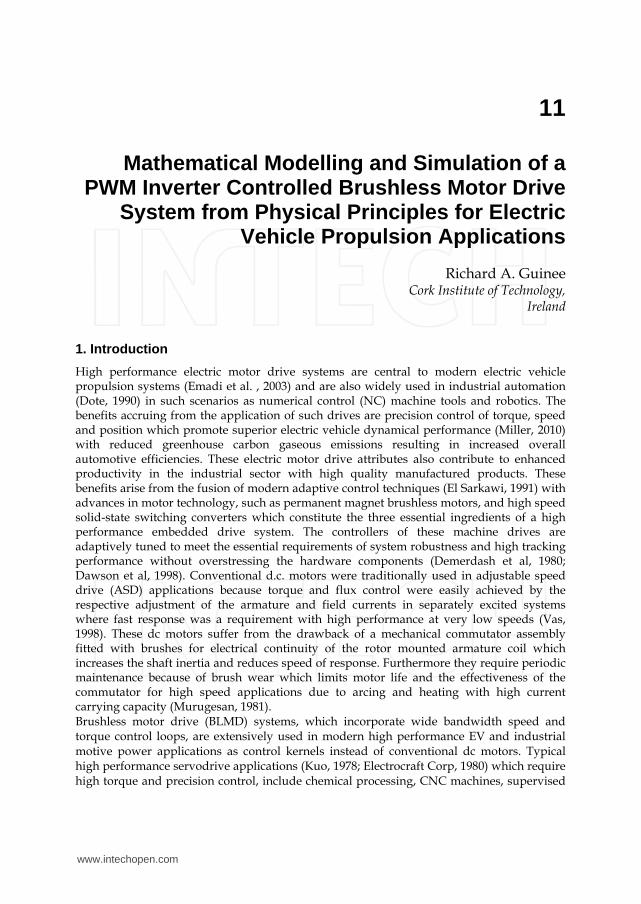
rotor displacement has been explained. The raison d’être of this simplifying assumption is that the permeability of the magnetically hard Samarium-Cobalt (SmCo5) material is almost equal to that of air. As a consequence of this property the SmCo5 material has some desirable features from a BLMD modelling perspective in terms of its intrinsic demagnetization characteristic. The PM rotor air gap line (Matsch, 1972) is a design feature which is optimized in terms of the maximum energy product of 160 kJm-3 (Crangle, 1991) for a given machine configuration and magnet geometry. In Figure 7 the locus of operation of the air gap line, due to changes in gap width, is a minor hysteresis loop (Match, ibid) with axis
tangent to the magnetization curve through the retention flux 0.
B
Retentivity BR
Flux 0
Air gap Linesgmax gmin
HCoercitivity Hc
(B, )
Intrinsic DemagnetizationCharacteristic
Bmax
BH
Energy ProductCharacteristic
BHmax
Fig. 7. PM flux variation with air gap width
The corresponding oscillating PM flux variations , which occur p times per rotor
revolution, are practically negligible (0) with little impact on the overall rotor flux linkage contribution to the stator windings.
Hc max
B
Retentivity{ BR ,0}
Retentivity{ BR ,0}
Air gap Line
Intrinsic DemagnetizationCharacteristic
2
3
1
Demagnetizing Field H
Hysteresis Loop
Fig. 8. Demagnetizing MMF effect
www.intechopen.com

Mathematical Modelling and Simulation of a PWM Inverter Controlled Brushless Motor Drive System from Physical Principles for Electric Vehicle Propulsion Applications
251
In Figure 8 the repeated application of a demagnetizing MMF, generated by the stator windings, results in a negligibly small flux variation (0) associated with the minor hysteresis loop on the demagnetization curve. The applied radial stator H-field, which is designed to lie on the knee of the intrinsic demagnetization characteristic (Pesson et al, 1976) corresponding to the energy product figure BHmax, has its maximum value associated with the air gap line at Hmax. Since the PM relative permeability (r) is almost unity, the applied field generated in the stator windings is not affected by rotor position.
2.2.3 Electromechanical energy conversion and torque production In a BLMD system the electromechanical energy conversion process involves the exchange of energy between the electrical and mechanical subsystems through the interacting medium of a magnetic coupling field. This energy transfer mechanism is manifested by the action of the coupling field on output mechanical motion of the rotor shaft masses and its stator winding input reaction to the electrical power supply. This reaction, which is necessary for the coupling field to absorb energy from the electrical supply, is the emf Vs
(t) induced across the coupling field by the magnetic field interaction of the stator winding with the PM rotor. Energy conversion during motor action is maintained by the incremental supply of internal electrical energy dWe, associated with sustained current flow Is(t) against the reaction emf, to balance the differential energy dWf absorbed by the reservoir coupling field and that released by the coupling field dWm to mechanical form. This results in the replenished energy transfer for sustained motion with stator flux change ds(I,r), using (V), as
*e t t dt t d ( , ) s s s s r f mdW I V I I dW dW (XXVI)
where mechanical and field losses are included in the electrical source Vs(t) and are thus
ignored for convenience. In a motor system most of the stator winding MMF is used to overcome the reluctance of the air gap separating the fixed armature from the moving rotor in the magnetic circuit. Consequently most of the magnetic field energy is stored in the air gap so that when the field is reduced most of this energy is returned to the electrical source. Furthermore since stacked ferromagnetic laminations are used in the stator winding assembly the magnetic field core losses are minimal whereupon the magnetic coupling fields are assumed conservative. The field energy state function Wf (1s,2s,3s,r) can be expressed in terms of the flux linkages (1s,2s,3s) in (XVI), for multiple stator winding controlled excitations with appropriate index change, and the mechanical angular displacement r of the rotor. This can be expressed in differential form using (XXVI) in terms of the stator winding flux linkages js and currents ijs as
3 3
1 1
f f
js r
W W
f js r js js mj jdW d d i d dW
(XXVII)
The mechanical energy transfer dWm with incremental change dr in rotor position r due to developed electromagnetic torque e(Is,r) by the coupling field is expressed by
,m e r rdW d sI (XXVIII)
By coefficient matching the state variables r and js for j{1,2,3} in (XXVII) and (XXVIII) an analytical expression for the electromagnetic (EM) torque e is obtained with
r
rfWre
),(),( s
s� . (XXIX)
www.intechopen.com

Electric Vehicles – Modelling and Simulations
252
in terms of the coupling field stored energy as a function of the flux linkages s. The coupling field energy is first determined by integration of the other coefficient partial differential equations
}3,2,1{ ),(
jijs
rfWjs
s (XXX)
with respect to the flux linkages of the connected system for restrained rotor conditions as
,,,),( 31 321
),(
)0(s j rsssjsjsjsj
W
drf iiididWjs
rf
r
s (XXXI)
as shown in Figure 9 before evaluation of the drive torque. Since the flux linkages are functions of the stator winding current, complex and lengthy numerical integration of (XXX)
would be required over the nonlinear -i magnetization characteristic in Figure 9, which must be known, if saturation effects are to be included. However if magnetic nonlinearity is neglected, with the assumption that the flux linkages and MMFs are directly proportional for the entire magnetic circuit as in air, the resulting analysis and integral expression (XXXI) is greatly simplified. In this case the flux linkages are assumed to be linear with current magnitude, which is often done in the analysis of practical devices, in the winding inductances as in (XXII). However a simpler and more convenient alternative (Krause, 1986)
than obtaining the EM torque as a function of s via Wf(s,r) in (XXXI), relies on the
coenergy state function Wc(Is,r) to determine the applied torque e in terms of the stator currents Is as the independent PWM controlled state variables in BLMD system operation. This methodology is more effective during BLMD model simulation as the motor winding currents are immediately available for motor torque computation.
dijs
ijs
js
Energy Wf
Coenergy Wc
MagnetizationCharacteristic
djs
js
i js
Fig. 9. Stored energy and coenergy
The coenergy Wc(Is,r), which has no physical basis or use other than to simplify the torque
calculation, is the dual form of the coupling field energy Wf(s,r) as shown in Figure 9 with
rfT
rc WW ,ˆˆ, ssss II (XXXII)
www.intechopen.com

Mathematical Modelling and Simulation of a PWM Inverter Controlled Brushless Motor Drive System from Physical Principles for Electric Vehicle Propulsion Applications
253
The following equivalent expressions result for the differential forms of the coenergy in
(XXXII) using the substitutions (XVII) and (XVIII) for Wf(s,r)
3 3
1 1( , ) ,c r js js js js js js e r rj j
dW i d di i d d s sI I (XXXIII)
3
1, c c
js r
W Wc r js rij
dW di d sI (XXXIV)
which when coefficient matched yield the parametric equations
,
j {1,2,3}c rW
js
s
js
I
i (XXXV)
,, c r
r
W
e r
sI
sI . (XXXVI)
The coupling field coenergy is determined from (XXXV) by integrating the cumulative stator flux linkages in (XV) with respect to the appropriate phase currents for restrained rotor movement as
,3 3, 1 1
W Ic s rW I di dic s r j js j js jsi js
(XXXVII)
If magnetic nonlinear saturation effects and field losses are negligible then the flux linkages
are linearly related to the currents, which establish the magnetic coupling field, through the
inductance circuit elements as in (XIX) for a salient pole rotor with
3
1( )js jk ks jmkL i (XXXVIII)
The resulting coenergy Wc, from substitution of (XXXVIII) into (XXXVII), is given by
3 3 3 32112 1 1 10
, r
kc r jj js jk ks js jm jsj j jd k jW L i L i i i sI (XXXIX)
from which the EM torque is evaluated using (XXXVI) as
21 3 3 3 3 , 1 1 112
dL dL djj jk jmi i i ie r j js j ks js j jskd d dr r r
k j
Is (XL)
This may be expanded in terms of the stator winding inductances for a salient pole machine as
3 32( 1) 2( 1)2
13 31
3 2( 1)
31
, sin 2 2 sin 2
cos
j kke r G r js r ks jsj k j
jt r jsj
pL p i p i i
K p i
sI (XLI)
www.intechopen.com

Electric Vehicles – Modelling and Simulations
254
with torque constant Kt = pm which is the same as Ke if proper units are used. If a round
rotor structure is assumed, then the LG terms in (XLI) disappear and the resulting developed
motor torque, due to the coupling field reaction EMF, in general terms is given by
3 3 2( 1)
31 1
3 2( 1)
31
, cos
cos
jm
r
d je r js m r jsdj j
je r jsj
i p p i
K p i
sI (XLII)
or in a more compact general form, using (XVII), as
1, { ( )} ( , ) { ( )}r s r
T Td de r s sm r ss r sm rd L d sI I I (XLIII)
The first two terms in (XL), which vanish in (XLII), represent the reluctance torque that
tends to align the salient poles in the minimum reluctance position with rotating air gap
flux. Motor torque control in high performance industrial drives is achieved by an
electronically commutated 3-phase PWM inverter which forces the armature phase currents
ijs in (XLII) to follow the sinusoidal reference currents idj generated from a prescribed torque
demand signal i/p Γd using rotor position information r. In the 3 commutated BLMD
system in Figure 1A the reference sinusoids, issued from the phase generator, are amplitude
modulated (AM) by the i/p torque demand d or velocity error signal via a multiplying
DAC. This AM effect is reflected in winding current amplitudes Ijm which vary with time as
Ijm(t) in symphony with the current demand signals {Ida,Idb,Idc}. These winding currents can
be thus written in the following vector form, with amplitude variation included, as
112
2 2 32
3 3 3
( )cos( )
( ) ( )cos( )
( )cos( )
m es
s m e
s m e
I t ti
t i I t t
i I t t
sI (XLIV)
Consequently the developed torque is expressed by (XLII) in its most general form to allow
for current amplitude variations which track the i/p torque demand signal excursions
during transient step changes. Expression (XLII) is employed during BLMD model
simulation to compute the motor torque from the derived stator winding currents for
simulation of the rotor shaft drive dynamics. The steady state motor torque is determined
from (XLIII), for balanced 3 phase conditions with constant amplitude stator winding
currents as in (III), with
23 2( 1) 33 21
, cosj
e r e m r m ejK I p I K
sI (XLV)
The mechanical power Pm delivered by the magnetic coupling field can be determined from
the applied motor torque in (XLII) which holds the rotor drive shaft load at an angular
velocity r as
3 2( 1)
31cos
jm e r e r r jsj
P K p i
(XLVI)
www.intechopen.com

Mathematical Modelling and Simulation of a PWM Inverter Controlled Brushless Motor Drive System from Physical Principles for Electric Vehicle Propulsion Applications
255
This is identical to electrical power Pe provided to each of the stator phase windings
ignoring losses, by the PSU, in sustaining the magnetic coupling field from collapse during
mechanical energy transfer. The electric power is accomplished by means of phase current ijs
injection against coupling field back-emf reaction vej. The PSU contribution Pe is expressed
by means of (XIV) and (XLIV) as Te sV I with
3 2( 1)
31cos( ).
je m e r r jsj
P P K p i
(XLVII)
which defaults to (XLVI) for zero internal power factor angle I in the phasor diagram of
Figure 10 and for constant amplitude winding currents.
Rotor Flux
Reaction EMF VejArmaturereaction
Flux
jss
js mj
Phase Current
jXsI js
T
I js
Vej
Phase voltage Vjs
RsI jsI
Mutualairgap Flux
Round RotorLeakage Inductance Lls=0
Torque Angle T
Load Angle T
Internal Power Factor Angle I
Power Factor Angle
Fig. 10. Phasor diagram for PM motor
The physical manifestation of motor torque production, which is expressed as the product of stator current and the rotor air gap flux given in (XLIII), results from a tendency of the stator and rotor air gap flux fields to align their magnetic axes with minimum energy configuration. Consequently maximum torque is developed by the motor as in (XLIII) when the torque angle
, defined as the angle between the armature reaction ss(I,r) and PM flux sm(r) space vectors in (XVII), is maintained at 90 degrees. Optimum torque angle control can be achieved in a BLMD system by means of self synchronization, via a rotor shaft position resolver as shown in Figure 1, in which a current controlled PWM inverter ensures an orthogonal spatial relationship between the stator and rotor flux vectors. This can be visualized with the aid of
the phasor diagram in Figure 10 where the torque angle , given by
/ 2 I (XLVIII)
www.intechopen.com

Electric Vehicles – Modelling and Simulations
256
with internal power factor angle I for steady state conditions, is forced towards 90 degrees
by adjustment of the armature reaction field jss. This adjustment is accomplished with stator phase current Ijs angle control, via electronic commutation, which also implies that the
internal power factor angle I between the reaction EMF Ve and armature current Is in (XLVII) is held at zero.
The PM air gap flux mj generates a phase-j reaction EMF Vej in Figure 10 at steady state rotor
angular velocity r. This EMF has a maximum value for a given shaft speed when the phase winding axis is displaced 90 electrical degrees relative to the rotor flux axis in which case the phase winding conductors are opposite the rotor magnetic poles with zero flux linkage.
Consequently the emf phasor Vej lags the flux phasor mj by 90 degrees. The developed EM
torque e results in sustained mechanical motion of motor drive shaft against a coupled load
torque l, with angular velocity r, expressed by the torque balance differential equation as
( ) rde l m l m rdt
J J B (IL)
where Jm and Jl are the respective shaft and load moments of inertia and Bm is the motor
shaft friction or damping coefficient. The motor shaft position r is obtained from the rotor angular velocity by numerical integration during BLMD model simulation using
0
( )t
r r d (L)
The equations (XXIII) and (XXIV) governing the electrical behaviour and the dynamical expressions (XXXII), (IL) and (L), together with the Laplace transform, form the basis of a mathematical model shown in Figure 1 of a brushless dc motor for complete simulation of the drive system.
2.2.4 Modelling of BLMD power converter with inverter blanking Brushless motor speed or torque control is achieved by adjusting the amplitude and frequency of the stator winding phase voltages which are synchronized in phase with instantaneous rotor position. Several different methods of power converter operation in regulating the 3-phase motor winding voltage excitation have been reported in the literature (Murphy et al, 1989). The widely used method of ASD stator winding voltage control which relies on three-phase six-step inverter operation, with a basic 60 degree commutation interval over a 120 degree conduction mode and an adjustable dc link voltage, suffers from low order harmonics with resultant low speed motor torque pulsations (Jahns, 1984). An effective alternative to the six-step mode of operation relies on voltage control within the inverter using pulsewidth modulation. The PWM control strategy results in better overall transient response with the elimination of low frequency harmonic content and motor cogging if a large carrier to reference frequency ratio is employed. A wide variety of PWM techniques are available (Adams et al, 1975) such as synchronized square-wave (Pollack, 1972) and sinusoidal PWM (Grant et al, 1981, 1983) with the latter being the preferred choice in asynchronous form with a very large fixed carrier ratio in commercial applications. Smooth motor shaft rotation down to standstill is obtained via a sinusoidal asynchronous PWM inverter which delivers a high fidelity fundamental o/p voltage waveform to the stator windings. The accompanying distortion frequency components, due to modulated pulse shaping, are concentrated about the high frequency carrier and its harmonics and are easily attenuated by the stator winding inductances.
www.intechopen.com
Mathematical Modelling and Simulation of a PWM Inverter Controlled Brushless Motor Drive System from Physical Principles for Electric Vehicle Propulsion Applications
257
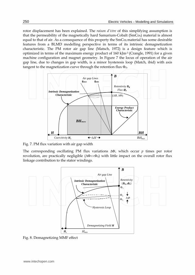
In a 3 current-controlled PWM inverter each current loop is equipped with a current controller and comparator modulator which provides wide bandwidth dynamic control of the stator current for high performance drive torque applications. Each current controller
is fed with a sinusoidal current command reference idj from the 3 current commutator, shown in Figure 1, along with the sensed stator winding current feedback ifj via Hall effect measuring devices. The rapidly adjusted error o/p vcj(t) from the current compensator forces the actual motor current ijs in each phase, via the high gain PWM controlled voltage-source inverter, to track the command reference in both phase and magnitude with minimal error. A mathematical model of 3-phase inverter operation can be obtained by describing the control action of the pulsewidth modulator in each phase, fed with a fixed voltage dc supply Ud, on the amplitude and frequency adjustment of the BLMD stator winding voltage in response to the current compensator error output. Modulation proceeds in two steps in accordance with the current controller output as shown in Figure 1. A symmetrical double edge width modulated pulse train is generated for each phase by means of a voltage comparator as the first step. A triangular carrier waveform Vtri(t), of fixed frequency fs and common to all three phases, establishes the switching period Ts and the current control error reference vcj(t) then modulates the switch duty cycle as shown in Figure 11 for phase-a.
-0.1 0.1 0.3 0.5 0.7 0.9 1.1 1.3-12
-7
-2
3
8
Pha
se_a
: V
olta
ge V
sa (
t) (
Vol
ts)
VsA
A: Modulating Current Control Signal Vca(t) = Vm(t) B: Base Drive PWM Waveform (No Delay) Vsa(t) C: Triangular Carrier Vtri(t) with peak Ad
Time (mS)
B C
MI=0.72 Ad=6.9 Volts Vm=5 Volts Fm=833Hz
-0.1 0.1 0.3 0.5 0.7 0.9 1.1 1.3-15
-10
-5
0
5
10
Sw
itch
Co
nto
l Vo
ltag
e V
sa(t
)
Time (mS)MI=0.72 Ad=6.9 Volts Vm=5 Volts Fm=833Hz
Vs
-Vs
TA+ ON
TA - OFF
TA+ OFF
TA - ON
Fig. 11. Comparator modulator waveforms Fig. 12. Phase-a switch control voltage
The modulated bipolar switch pulse train ( )sjv t is then used as the firing signal, at the
modulator o/p as shown in Figure 12 for phase-a, to control the “ON” and “OFF” periods
of the power transistors, via the base drive circuitry (BDA), in each half-bridge of the 3
inverter as the subsequent step. Similar switching sequences, with a phase angle separation
of 120 degrees, are obtained for control of the other two phases of the inverter bridge
resulting in a 3 PWM voltage supply to the motor stator windings. In practical inverters
the finite turn-off time of the power transistor bridge necessitates the use of a finite blanking
switch time in the PWM process to avoid short circuiting the dc busbar to ground (Murai,
1985; Evans et al, 1987; Dodson et al, 1990). This fixed ‘interlock delay’ , which is typically
20 µS, is conservatively chosen for slow switching Darlington transistors in medium power
motor drives in the low kilowatt range.
www.intechopen.com

Electric Vehicles – Modelling and Simulations
258
-0.1 0.1 0.3 0.5 0.7 0.9 1.1 1.3-5
0
5
10
15B
ase
Driv
e B
DA
Vol
tage
Vba
(t)
Time (mS)
Transistor TA +
Without Delay With Delay
Vs
MI=0.72 Ad=6.9 Volts Vm=5 Volts Fm=833Hz
20S
-0.1 0.1 0.3 0.5 0.7 0.9 1.1 1.3-5
0
5
10
15
Ba
se D
rive
BD
A V
olta
ge
Vb
a(t
)
Time (mS)
Transistor TA -
Without Delay With Delay
Vs
MI=0.72 Ad=6.9 Volts Vm=5 Volts Fm=833Hz
20S
Fig. 13. Base drive voltage for TA+ Fig. 14. Base drive voltage for TA-
This dwell time, between successive power transistor switching instants, is effected through
an integrate and dump RC ‘lockout’ network connected to a voltage threshold in the base
drive circuitry. A switching delay of this magnitude, for inverter frequencies in the audio
range (5kHz), has to be included in the motor drive modelling process for accurate
simulation studies. The effect of the switching delay can be modelled as follows by
considering phase-a only with a similar procedure for the other two phases (Guinee et al,
1998, 1999).
Fig. 15. Phase-j inverter operation Fig. 16. Regula-falsi iterative search
The duty cycle of the bipolar switch control voltage vsa(t), during one switching period Ts in
Figure 12 is determined by the relative magnitude comparison and accurate crossover
evaluation, from simulation via the regula-falsi iterative search method shown in Figure 16,
of the current control voltage vca(t) with the dither reference vtri(t). The switch control pulse
sequence can be described as
BASEDRIVE J BDJ
J
J
TJ+
TJ-
HT Busbar Ud
3 BASE DRIVE
Vlj
Vlj
Vbj
Vbj
Vjg
Three Phase Inverter Operation
Ijs <0
Ijs >0
TJ+ & TJ- in OFF mode
D j
D j
Iterative Step Size t
Regula Falsi Iteration method
PWM O/P
Time
PWM O/PCarrier
Vtri(t)
Signal Vcj(t)
tk-1 tktX t*
lvChord
Approx.
www.intechopen.com
Mathematical Modelling and Simulation of a PWM Inverter Controlled Brushless Motor Drive System from Physical Principles for Electric Vehicle Propulsion Applications
259
{ ( ) ( )}
( ) { ( ) ( )}
s ca trisa
s ca tri
V v t v tv t
V v t v t
(LI)
with modulated pulse duration
2
{ ( ) }
(1 ) {| | 1}
0 { ( ) }
s
s ca d
Tf f
ca d
T v t A
m m
v t A
(LII)
for carrier amplitude Ad and modulation index (MI) mf given by
( )f ca dm v t A (LIII)
The effect of the switch control voltage on the inverter base drive transistors TA+ and TA–
under ideal conditions, without delay is illustrated in Figures 13 and 14.
When blanking is introduced inverter switching is postponed until the capacitor voltages of
the complementary RC delay circuits, associated with power transistors TA+ and TA–,
exceeds the threshold level setting Vth in the base drivers as shown in Figures 13 and 14 and
detailed in Figure 17. The magnitude of the delay , typically 20µS, is given by
2
ln( ) 0.693 if 0s
s th
VthV V
RC RC V (LIV)
When phase-a power transistors TA+ and TA–, are “OFF” during the blanking period winding current conduction is maintained through free-wheeling protection diodes, as shown in Figures 1 and 15, so that each transistor with its accompanying antiparallel diode functions as a bilateral switch. The relationship between the states of the dc to ac converter
phase-a switch transistor pair, denoted by SA(k) with k{0,1,2}, and the base drive voltages
& la lav v in Figure 17 can be represented by
( ) 0 is "OFF"(0)
( ) is "ON"
( ) is "ON"(1)
( ) 0 is "OFF"
( ) 0 is "OFF"(2)
( ) 0 is "OFF"
la th ba AA
la th ba B A
la th ba B AA
la th ba A
la th ba AA
la th ba A
v V v t TS
v V v t V T
v V v t V TS
v V v t T
v V v t TS
v V v t T
(LV)
with similar expressions SJ(k) and J{A,B,C} for the other two phases. The power
transistors in each leg of the inverter are thus alternately switched “ON” and “OFF”
according to the tristate expression (LV) with a brief blanking period separating these
switched transistor conduction states. The tristate operation of the power converter bridge
also determines the phase potential i/p of the stator winding as a result of the PWM
gating sequence applied to the basedrive in (LV). The corresponding converter voltages
applied between the stator phase winding input connection and ground, denoted by vag,
vbg, and vcg, are then given by
www.intechopen.com

Electric V
ehicles – Modelling and S
imulations
260
Fig
. 17. Tran
sfer Fu
nctio
n B
lock
Diag
ram o
f a BL
MD
Sy
stem (G
uin
ee, 1999)
Pulse Width Modulator
-+ Current
Filter HDI
vcj
3Current Commutation
Filter HT
Velocity Controller GV
Shaft Velocity Filtering
Idj
Position Resolver
RC Delay
vlj=-Vs,vsj<0
,vsj0 1+sRC1
=-Vs,vsj0 v lj
,vsj0 1+sRC1
Base Drivevbj=VB,vljVth
=0 ,vljV th
V th V th
v lj=VB, =0 ,v lj
v bj
v bj
Inverter State Sj(*)
Sj(0) {vbj=0, Sj(1) {vbj>0, Sj(2) {vbj=0,
>0} =0} =0}
v bj
v bj
v bj
vlj
v lj
vbj
v bj
Triangular Carrier
Inverter Output
vjg=Ud
vjg=0
{Sj(1) Sj(2) & ijs<0Sj(0) Sj(2) & ijs>0{
Stator Winding Phase Voltage:
vjg
vjs+
Stator Winding
Kt
l
+Motor Dynamics e
- vej
Torque Constant
Back EMF Constant
Current Feedback
Ias
Ifj
+
-
Legend
Test PointPhase j={a1,b2,c3}
Vtri
V sj =Vs, vcj v tri
-V s, vcj v tri
PWM O/P
V sj
Vr
Kc1s a1s b
Filter HFI
KF
1 s F
Kwi
Current Demand
KI1sd
sin pr 2( j 1) 3
1 s
Torque Demand
KT1sT
Kp K I s
d
HVoo2
S2 oS o2
V
V js V jg Vsg
Vsg 13 V jgj
1r s sLs
sin pr 2( j 1) 3 j
1Bm sJm -
sin pr 2( j 1) 3 r
r
Ke
controller GI
ww
w.intechopen.com
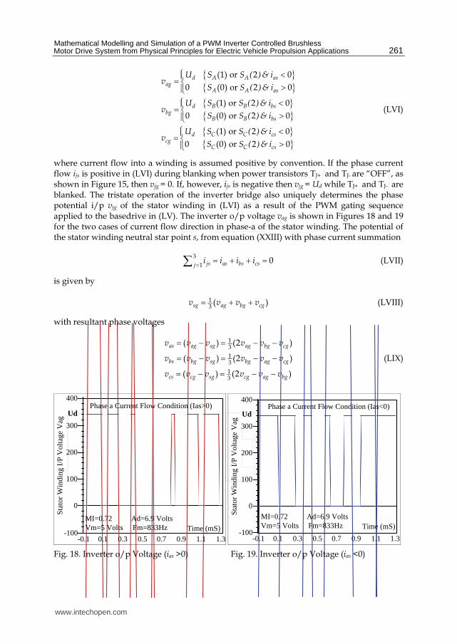
Mathematical Modelling and Simulation of a PWM Inverter Controlled Brushless Motor Drive System from Physical Principles for Electric Vehicle Propulsion Applications
261
(1) or 2 0
0 (0) or 2 0
(1) or 2 0
0 (0) or 2 0
(1) or 2 0
0 (0) or 2 0
d A A asag
A A as
d B B bsbg
B B bs
d C C cscg
C C cs
U S S ( ) & iv
S S ( ) & i
U S S ( ) & iv
S S ( ) & i
U S S ( ) & iv
S S ( ) & i
(LVI)
where current flow into a winding is assumed positive by convention. If the phase current flow ijs is positive in (LVI) during blanking when power transistors TJ+ and TJ- are “OFF”, as shown in Figure 15, then vjg = 0. If, however, ijs is negative then vjg = Ud while TJ+ and TJ- are blanked. The tristate operation of the inverter bridge also uniquely determines the phase potential i/p vjg of the stator winding in (LVI) as a result of the PWM gating sequence applied to the basedrive in (LV). The inverter o/p voltage vag is shown in Figures 18 and 19 for the two cases of current flow direction in phase-a of the stator winding. The potential of the stator winding neutral star point s, from equation (XXIII) with phase current summation
3
10js as bs csj
i i i i (LVII)
is given by
13
( )sg ag bg cgv v v v (LVIII)
with resultant phase voltages
13
13
13
( ) (2 )
( ) (2 )
( ) (2 )
as ag sg ag bg cg
bs bg sg bg ag cg
cs cg sg cg ag bg
v v v v v v
v v v v v v
v v v v v v
(LIX)
-0.1 0.1 0.3 0.5 0.7 0.9 1.1 1.3-100
0
100
200
300
400
Sta
tor
Win
ding
I/P
Vol
tage
Vag
Time (mS)
Phase a Current Flow Condition (Ias>0)Ud
MI=0.72 Ad=6.9 Volts Vm=5 Volts Fm=833Hz
-0.1 0.1 0.3 0.5 0.7 0.9 1.1 1.3-100
0
100
200
300
400
Sta
tor
Win
ding
I/P
Vol
tage
Vag
Time (mS)
Phase a Current Flow Condition (Ias<0)Ud
MI=0.72 Ad=6.9 Volts Vm=5 Volts Fm=833Hz
Fig. 18. Inverter o/p Voltage (ias >0) Fig. 19. Inverter o/p Voltage (ias <0)
www.intechopen.com

Electric Vehicles – Modelling and Simulations
262
The complete three phase model of a typical high performance servo-drive system (Moog GmbH, 1989; Guinee, 1999). incorporating equations (XXIII), (XXIV), (XLII), (IL), (L), (LV), (LVI) and (LIX), used in software simulation for parameter identification purposes is displayed in Figure 17.
3. Numerical simulation accuracy and experimental validation of BLMD model
Since the BLMD model is partitioned into linear elements and non linear subsystems, owing to the complexity and discrete temporal nature of the PWM control switching process, numerical integration techniques have to be applied to obtain solutions to the differential electrodynamic equations of motion. Numerical simulation of the continuous-time subsystems, with a transfer function representation based on the Laplace transform, is achieved by means of model difference equations with numerical solutions provided by the use of the backward Euler integration rule (BEIR) (Franklin et al, 1980). In this instance continuous time derivatives are
approximated in discrete form using the Z Transform substitution operator 11 (1 )T
S Z .
Since the BEIR maps the left half s-plane inside the unit circle in the z-plane these solutions are stable. The choice of this implicit integration algorithm is based on its simplicity of substitution, ease of manipulation with a small number of terms and reduced computation effort in the overall complex BLMD model simulation. An alternative filter discretization process based on Tustin’s bilinear method, or the trapezoidal integration rule with the
substitution operation )1()1( 112 ZZST
, can be implemented with negligible
observable differences at the small value of integration step size T actually chosen. The application of the BEIR technique can be visualized for a first order system, as in the case of the current control lag compensator GI which has a generalized transfer function (Guinee, 2003)
0 1
0 1
1( )
( ) 1( ) a
b
s sV sI cI s s s
G s K K , (LX)
with continuous-time description given by
( ) ( )0 1 0 1( ) ( )
dV t dI t
dt dtV t K I t (LXI)
Integrating (LXI) between the discrete time instants tk and tk-1 with a fixed time step size T gives
1 1
1 1 1 1 1 1 0 0( ) ( ) ( ) ( ) ( ) ( )k k
k k
t t
k k k k t tV t K I t V t K I t K I d V d
(LXII)
Applying the BEIR, with piecewise constant integrand backward approximations V(tk) and
I(tk) over the interval tk t > tk-1 yields the input-output difference equation
1 0 1 1 1 0 1 1( ) ( ) ( ) ( )k k k kV t T V t K T I t K I t (LXIII)
This can be expressed in the Z domain, via the Z Transform, as the transfer function
11 10 1 0 1
1110 10 1
1( )
( ) 1
T
T
Z n n ZV Z
I Z d d ZZK k
(LXIV)
www.intechopen.com

Mathematical Modelling and Simulation of a PWM Inverter Controlled Brushless Motor Drive System from Physical Principles for Electric Vehicle Propulsion Applications
263
which is equivalent to (LX) through the general BEIR substitution operator 11 (1 )T
S Z .
The time evolution of each discretized linear subsystem proceeds according to the BEIR, similar to (LXIII), as an integral part of the overall BLMD numerical simulation with a fixed
time step T=t and input x(t) to output y(t) relationship given by
11 1
0 00 1( )k k k
dk kd d
y n x n x y (LXV)
The choice of time step size is determined by the resolution accuracy of the PWM switching instants required during simulation for delayed inverter trigger operation as explained in section 3.1 below. The BLMD model program is organized into a sequence of software function calls, representing the operation of the various subsystems.
3.1 PWM simulation with inverter delay The choice of numerical integration step size t, for solution of the set of dynamic system
differential equations, is influenced by the PWM switching period TS (≈200S) (Moog, 1989)
and the smallest BLMD time constant d (~28.6S) associated with the basedrive ‘lockout’ circuitry. Furthermore the precision with which the pulse edge transitions are resolved in the three phase PWM o/p sequences as in (LI) with inverter blanking included, has a significant effect on the accuracy of the inverter o/p waveforms. This is important in BLMD simulation where model accuracy and fidelity are an issue in dynamical parameter identification for optimal control. The effect of inaccuracy in pulse time simulation can be reduced by choosing a sufficiently small fixed time step ∆t << Ts, such as 0.5%TS or 5% of
the inverter dead time (≈20S) for example, to reflect overall BLMD model accuracy and curtail computational effort in terms of time during lengthy simulation trial runs.
Furthermore this choice of step size also provides an uncertainty bound of +t in the evaluation of PWM switching instants during simulation in the absence of an iterative search of the switch crossover time. This uncertainty can be reduced by an iterative search of
the PWM crossover time t* within a fixed assigned time step size t during BLMD simulation for which a width modulated pulse transition has been flagged as shown in Figure 16. A variety of iterative search methods can be employed for this purpose with varying degrees of computation runtime required and complexity. These include, for example, successive application of the bisection method, regula falsi technique and the Newton-Raphson approach (Press et al, 1990) where convergence difficulties can arise with derivative calculations from noisy current control signals. The number of iterations n
required for the bisection technique, with a fixed time step t, to reach an uncertainty in the pulse transition time estimate tX, is given by the error criterion
( 1)2 nt (LXVI)
The estimate of the PWM switching time t* obtained via the regula falsi method, from the comparison of the triangular carrier ramp with the piecewise linear approximation of the control signal vcj as shown in Figure 16, is given by the iterative search value tX as (Guinee, 1998, 2003)
1 1
1 1
{ ( ) ( )}
1{ ( ) ( )} { ( ) ( )}
tri k cj k
tri k cj k tri k cj k
v t v t t
kv t v t v t v tXt t
(LXVII)
www.intechopen.com

Electric Vehicles – Modelling and Simulations
264
The adoption of a single iteration of the regula falsi method along with a small simulation time step t simplifies the search problem of the pulse edge transition with sufficient accuracy without the expenditure of considerable computational effort for a modest gain in accuracy by comparison with the other iterative methods available. An indication of the step size required for accurate resolution of PWM inverter operation with delay can be obtained from consideration of the anticipated signal ‘curvature’ due to (a) the signal bandwidth and amplitude at the current controller o/p vcj in the magnitude comparison with the triangular carrier shown in Figure 16 in the comparator modulator and (b) the rate of exponential voltage ramp up to the base drive threshold Vth, which controls the inverter dead time, in the RC delay circuits shown in Figure 20. The maximum harmonic o/p voltage from the high gain current compensator GI is determined by the carrier amplitude Ad at the onset of overmodulation (mf = 1) in PWM inverter control with a frequency that is limited by the 3dB bandwidth F = 1/F (~3kHz in Table I) of the smoothing filter HFI in the current loop feedback path shown in Figure 17. This may be represented in analytic form as
( ) sin( )cj d Fv t A t (LXVIII)
VljVlj
0 50 100 150 200 250-25
-20
-15
-10
-5
0
5
10
Bas
e_D
rive
Vol
tage
s V
olts
Time (uS)
Vs
-Vs
CR
Comparator o/p Vsj
Base Drive i/p Vlj
Base DriveThreshold Vth
Base Drive Voltage Vlj Complementary Base Drive Voltage Vlj
TJ+ ON TJ- OFF
TJ+ OFF TJ- ON
Iterative Step Size t
Basedrive
Time
tk-1 tktX
Threshold Vth
Basedrive exponential Vlj
Piecewise Linear Approximation
t**
Fig. 20. Delayed basedrive trigger signals Fig. 21. Basedrive Trigger Time Search
with a quadratic power series approximation about the mid interval point t̂ in t given by
ˆ( ) 2
2!ˆ ˆ ˆ ˆ( ) ( ) ( )( ) ( )
cjv t
cj cj cjv t v t v t t t t t . (LXIX)
The accuracy with which the estimated width modulated pulse transition instants tX are determined can be gauged by comparing the deviation error of the actual intersection time t* of the triangular carrier with the control signal vcj, due to its curvature, to that tX obtained with the piecewise linear chord approximation of the signal in the regula-falsi method as illustrated in Figure 16. The ‘curvature’ of the signal in (LXVIII) with time, determined (Kreyszig, 1972) from
21cj cjv v , (LXX)
www.intechopen.com

Mathematical Modelling and Simulation of a PWM Inverter Controlled Brushless Motor Drive System from Physical Principles for Electric Vehicle Propulsion Applications
265
is given by its maximum value
2max cj d Fv A (LXXI)
at the peak amplitude Ad of vcj(t) corresponding to the instant 2 Ft in Figure 16 at
which ( ) cos( ) 0cj d F Fv t A t . The peak deviation lV of the signal due to curvature from
the chord approximation through tk-1 in Figure 16 occurs at t̂ t with zero chord slope. The
peak deviation from the chord, through 1 ( 2)kt t t , is determined by the Taylor series
expansion in (LXIX) about t̂ t with
22( ) 11 2! 2 2 2
( ) ( ) 1cj F
v t ttcj k cj dv t v t A
(LXXII)
giving
21 2 2( ) ( ) d FA t
v cj cj kl v t v t . (LXXIII)
The worst case deviation error of the pulse transition time estimate tX from t is determined
by the regula-falsi method at the point of intersection tX of the carrier ramp, which passes
through the signal coordinates [t, vcj(t)] in Figure 16, with the chord approximation to the
signal. The approximation error (t - tX) is determined from the ramp, which has peak-to-
peak excursion 2Ad over the half period TS/2, with slope m = 4Ad/TS as
2
8 2v s Fl T t
x mt t
(LXXIV)
Substitution of the set of relevant signal parameters { , , }S d FT A f , for a step size of 1s, with
values {200 , 6.9V, 3kHz}s result in a negligible approximation error relative to the step
size t of 0.222% which verifies the suitably of the chosen step size for a linear search of the
PWM crossover time. The PWM resolution accuracy determines the moment that a
modulated pulse edge transition takes place with subsequent onset of inverter blanking,
using lockout circuitry, which substantially affects power transfer from the dc supply to the
prime mover. The next essential trigger event, that needs to be accurately resolved, is the
instant at which retarded firing of the inverter power transistors commences when the RC
delay growth voltage exceeds the basedrive threshold Vth= 0 in Figure 20. The
complementary exponential trigger voltages & lj ljv v supplied to the basedrive circuitry, for
a modulator peak-to-peak o/p swing of 2VS, can be expressed as
(1 2 )t RClj sv V e . (LXXV)
The basedrive turnon time t** is given by (LIV) as (~19.82S), at the instant at which
( )lj thv t V , for a time constant d (~28.6S). Since delay circuit simulation is employed the
trigger instant tX has to be obtained using piecewise linear approximation of the exponential
growth waveform, within the flagged simulation interval as shown in Figure 21, and is given by
1
1
( )
1 ( ) ( )
lj k
lj k lj k
v t
x k v t v tt t t
(LXXVI)
www.intechopen.com

Electric Vehicles – Modelling and Simulations
266
where 1k kt t tx and **1 k kt t t . Assume that t** occurs at the mid interval time
1( 2)kt t which thus provides an absolute point of reference for comparison with the
search estimate tX. The effect of basedrive signal ‘curvature’ on the trigger estimate tX can be
gauged by monitoring the relative contribution of the quadratic terms in the Taylor series
expansion about t** as
( ) 22!
( ) ( ) ( )( ) ( )ljv t
l l lx x xv t v t v t t t t tj j j
(LXXVII)
with vlj(t**) = Vth = 0. The differential error in the crossover time estimate in (LXXVI) is
given by
2
2 2
31 12
( ) 4.37 10t
RC
t tRC RC
ex
e e
t t t t
(LXXVIII)
and is practically zero for very small time steps which implies a negligible quadratic contribution. Consequently the trigger time estimate obtained by linear approximation of the basedrive voltage about the threshold is very accurate for the time step size chosen.
3.2 Motor dynamic testing and simulation The steady state controlled torque versus output speed characteristic (Moog, 1988) for the
particular motor drive concerned is almost constant over a 4000 rpm speed range for a rated
continuous power o/p of 1.5kW. The corresponding dynamic transfer characteristic of o/p
motor torque e versus input torque demand d voltage is practically linear in the range (0,
10) volts. A fixed step signal d i/p is chosen to provide persistent excitation, as a standard
control stimulus for dynamic system response testing, and in particular to gauge the
accuracy of the model simulation and parameter extraction process based on the feedback
current (FC) response ifj. This response has the transient features of a constant amplitude
swept frequency sinusoid, during the acceleration phase of the motor shaft, which are
beneficial for test purposes and BLMD model validation in system identification (SI). The
phase current feedback simulation can then be checked against experimental test results as
the observed target data, for example in phase-a, for both phase and frequency coherence in
model validation. Further model validation is provided by the accuracy with which high
frequency ripple in the unfiltered current feedback is replicated through BLMD simulation
when compared with experimental test data. Examination of the presence of dead time
related low frequency harmonics in the simulated current feedback is also used to gauge
BLMD model fidelity, through FFT spectral analysis, when compared with measurement
data. An input magnitude of 1volt is sufficient to guarantee linear operation and avoid
saturation (mf >1) of the PWM stage by the high gain current controller chosen here as the
optimizer module MCO 402B in Table 1. This input step size is also enough to slow down
the rate of shaft speed ramp up to allow adequate resolution of the frequency change in the
FC target data.
The intrinsic mechanical parameters of motor viscous friction Bm and shaft inertia Jm are initially determined from experimental motor testing and cost surface simulations based on the mean squared error (MSE) between the simulated and measured transient response data for shaft velocity and current feedback. Two examples of known shaft load inertia JL are
www.intechopen.com

Mathematical Modelling and Simulation of a PWM Inverter Controlled Brushless Motor Drive System from Physical Principles for Electric Vehicle Propulsion Applications
267
then used in simulated response measurements as a check against BLMD test data for further model accuracy and validation. These simulation results, which correspond to the different inertial loads, are integrated into a parameter identification process, using MSE cost surface simulation, based on a Fast Simulated Diffusion (FSD) optimization technique for the purpose of motor drive shaft parameter extraction. The experimentally determined parameter values listed in Table II for the BLMD model are used in all model simulations. The back EMF or voltage constant Ke was experimentally determined from an open circuit (o/c) test with the motor configured as a generator driven over a range of speeds by an identical shaft coupled BLMD system. The generator voltage characteristic Vg is linear with
drive shaft speed m as shown for the experimental data in Figure 22, according to (XXIV), with slope Ke derived from the fitted linear voltage relationship Vf. The transducer velocity ‘gain’ GRDC of the Resolver-to-Digital Converter (RDC) was
concurrently estimated along with Ke from the slope of the fitted linear characteristic Vf, which in addition substantiates the converter linearity, to the speed voltage measurements shown in Figure 23. This value along with the cascaded shaft velocity filter gain is given as the cumulative gain Hvo in Table II.
Torque Demand Filter HT
KT =1.0; T =222S Voltages Ud =310 Volts; Vth =0;
VS =10 Volts
Current Demand Filter HDI
KI =1.0; I =100S Constants Kwi =6.8x10⁻²; Ke = Kt =0.3
Current Feedback Filter HFI
KF =5.0; I =47S Winding P =6; rS =0.75 Ohms;
LS =1.94mH
Basedrive Delay Circuit RC =28.6S Carrier fS =5kHz; Ad =6.9 Volts;
Current Controller Type High Gain: MCO 402B Low Gain: MCO 422
KC =19.5; a =225s; b =1.5ms
Motor Dynamics
Jm =3 kg.cm2;
Bm =2.14x10⁻³Nm.rad-1.sec KC =5.0; a =223S; b =0.7mS
Shaft Velocity Filter HV
Hvo =13.5x10⁻³;
=√2;
o =2x10³ rad.sec-1
Inertial Loads
JMML=9.06 kg.cm2 (Medium Mass –MML)
* JLML=17.8 kg.cm2
(Large Mass – LML)
*Returned Parameter Estimates: 2ˆ ˆ 20.838 kg.cmopt m LMLJ J J ,
3 -1ˆ 1.959 10 Nm.Sec.RadoptB x
* Simulated FC Response Surface Estimates: Jopt =20.877 kg.cm2, Bopt =1.921x10 Nm.Sec.Rad-1
Table II. BLMD system parameters
www.intechopen.com

Electric Vehicles – Modelling and Simulations
268
100 200 300 400
50
100
150
Rotor Shaft Angular Velocity r
Fitted Voltage Vf
Generated voltage Vg
Rads/sec
Open Circuit Voltage TestVOLTS
Slope =0.315=
EMF Constant Ke
200 400 600
0
2
4
6
Motor Shaft Velocity r0 Rads/sec
VOLTS
Shaft Speed Voltage Test
Shaft Speed VFitted VoltageVf
Slope= GRDC =1.16x10⁻³
RDC Voltage Gain
Fig. 22. Estimation of EMF constant Ke Fig. 23. Estimation of RDC ‘gain’ GRDC
The value of Ke was subsequently used in a motor-generator electrical load test, at different speeds as illustrated in Figure 24, to estimate the stator winding parameters Ls and rs as a cross check of the nominal catalogued (Moog, 1998) values. The difference V between the measured terminal voltage VT, across the load resistance RL, and the generated voltage VG using the fitted coefficient Ke via (XXIV) is equated to the internal voltage drop of the Thevenin equivalent circuit shown in Figure 24 with
| |G T LV V V Z I (LXXIX)
where
/L T LI V R .
50 100 1500
20
40
60
80Generator Electrical Load Test
Rheostat Load RL=18.3EMF Constant Kt =0.315
Shaft Speedr
Rads/sec
~
ZI
RLVTVG
IL
0
VOLTS
Terminal Voltage VTGenerator Voltage VG
50 100 150
0
2
4
6
8
0
Motor - Generator Electrical Load Test
Shaft Speed r
Rads/sec
Terminal Voltage VTGenerated Voltage VGDifferential VoltageV = VG - VT
Internal Voltage Drop VI = ZI ILParameter Estimatesrs =0.724; Ls =1.945mH
VOLTS
Fig. 24. Motor - generator load test Fig. 25. Winding parameter estimation
www.intechopen.com

Mathematical Modelling and Simulation of a PWM Inverter Controlled Brushless Motor Drive System from Physical Principles for Electric Vehicle Propulsion Applications
269
The quadratic polynomial expressed in terms of e via the circuit parameters as
2 2
0 0 eZ a b w , (LXXX)
for e = pr and constant coefficients a0 r2s and b0 L2s, is fitted to the derived data y =
(V/IL)2. The quadratic fit shown in Figure 25 is based on the minimization of the MSE (E), between the sampled yk and simulated Zk2 data, as
2
210 01
for N
k k eN kE y a b x x (LXXXI)
with respect to a0 and b0. The cost function minimisation results in the normal equations
2 2
22 2 20
Tk kk k
T
kk
x y NY X
x X Xb
(LXXXII)
21
0 0k kN k ka y b x (LXXXIII)
with parameter estimates ˆ 1.945mHsL and ˆ 0.724 ohmssr that are very close to the
nominal values in Table II. The motor shaft friction coefficient Bm was obtained from the steady state current feedback
Ifa in phase-a at various shaft speeds r by means of the torque constant Kt which is numerically equal to the experimentally determined value of Ke when proper units are used. The active component of the steady state current feedback is considered in the calculation of
the dissipative friction torque by allowing for the effect of the machine impedance angle Z increase, given by
1 1s js r s
s js s
X I p Lz r I r
Tan Tan , (LXXXIV)
with motor shaft speed and zero load angle T in Figure 10. This is necessary in electronic commutated motor drive systems, in which the current controlled applied phase voltage vjs at zero load angle is derived from the current demand Idj in Figure 17, without the benefits of adaptive current angle advancement (Meshkat, 1985) to counteract the torque reduction effects of internal power factor angle illustrated in Figure 10. The derived friction torque,
from the adjusted measured current feedback Ifa cos z, is given by
3 32 2
cos cost
wi f
Kf t as z fa zK K
K I I (LXXXV)
via (XLV) for balanced 3-phase conditions where the current feedback factor Kwi and filter gain Kf are considered in the estimation of the stator current flow Ijs. This is graphed in Figure 26 for the measured FC test data Ifa and equated to the steady state mechanical friction torque via (IL) as
f m rB . (LXXXVI)
www.intechopen.com

Electric Vehicles – Modelling and Simulations
270
100 200 300 400
0.5
1
Shaft Velocity m
Rads/sec
Motor Testing for Shaft Friction Bm
EstimationFriction Torque f estimation
via FC Ifa
Fitted estimatef
Friction Coefficient Estimate .Bm 2141 103 Nm.rad-1
200 400
200
400
600
Rads/sec
Shaft Velocityr
Shaft Friction Bm Estimationfrom Power Considerations
Mechanical Pow - Estimn Pm
Electrical pow - Estimn Pe
Watts
Fig. 26. Friction parameter estimation Fig. 27. Friction power estimation
The friction coefficient Bm is obtained from a linear first order polynomial fit, displayed in
Figure 26, based on expression (LXXXVI) with estimate 3 -1ˆ 2.141 10 Nm.radmB as in
Table II. Alternative confirmation of the accuracy of the damping factor estimate is obtained
from consideration of the electrical power transfer Pe from the coupling field expressed in
(XLVII) and comparison with the resultant mechanical power dissipation Pm associated with
dynamic friction via (XLVI). The continuous power supplied from the coupling field,
necessary to sustain motor rotation with frictional losses at various shaft speeds under
steady state conditions, is determined from the rms values of reaction EMF using the
measured estimate ˆeK from the o/c test and the experimental FC test data with lagging
power factor balanced over three phases as
ˆ
2 23 cos
fa e r
wi f
I Ke zK K
P . (LXXXVII)
The mechanical power dissipated as frictional heat is evaluated from (LXXVI) using the
measured estimate ˆmB as
2ˆm f r m rP B (LXXXVIII)
Both power estimates exhibit a high degree of correlation, with correlation coefficient
(Bulmer, 1979) of 99.5%, when plotted in Figure 27 which validates the derived damping
factor estimate ˆmB .
3.3 Motor step response testing and simulation results Synchronized initial conditions for BLMD testing, and resultant comparison with model numerical simulation, are obtained by hand cranking the motor shaft to top dead centre of the phase-a current commutation reference position while monitoring the phase generator o/p waveforms before application of the torque demand step i/p. This is essential for
www.intechopen.com

Mathematical Modelling and Simulation of a PWM Inverter Controlled Brushless Motor Drive System from Physical Principles for Electric Vehicle Propulsion Applications
271
proper datum time referencing of all waveforms in the eventual comparison process, when formulating a multiminima cost surface for minimization purposes using the least squares error criterion, during parameter identification.
Torque Demand
cos(pr-2(j-1)/3)
Gv 3 Current Commutation
3Current Command Filtering
HDI
3Current Controller
Idj
GI +-
3PWM Modulator
Triangular Carrier Vtri
Vcj
3 Delay Network j
BDj
Tj+
Tj- 3BASE DRIVE
Ijs
Filtering HFI
Hall Effect Device HED
3Current Feedback
Phase Generator ROM Table
Shaft Velocity Filter Hv
Position r
Velocity Feedback r
Velocity
V
d
Lss
3Stator windingHT Busbar Ud
3 PWM INVERTER
rs
HT
RC
j
Command
Filtering
Controller
Vsj Vjg
Vbj
Vbj
PM Rotor P pole Pairs
Shaft Inertia Jm
Friction BmShaft Position Resolver
-
+
Ifj
r
Fig. 28. Network structure of a typical BLMD system
The actual drive system with network structure as shown in Figure 28 was tested at critical internal nodes with multiplexed sampled data waveforms acquired at rates corresponding to the different inertial loaded shaft conditions (JL ) specified in Table III. The length of each data record is fixed at 4095 sample points with a normalized duration of approximately 10 machine FC cycles for reference purposes during comparison with simulated motor response for model validation and accuracy and also during system identification for accurate extraction of drive motor model parameter estimates.
FC Target Data No. of machine cycles Acquisition rate T
No. of data points Nd
No Shaft Load (NSL) ~ 9.75
20s 4095
Medium Inertial Load (MML) ~ 11.5
40s 4095
Large Inertial Load (LML) ~ 10.5
49.6s 4095
Simulation time step Decimation Factor
1s 20
1s 40
1s 50
Waveform Correlation Analysis for BLMD system without inertial shaft loads
Signal x Exp Ixa Sim ixa Data Correlation Coefficient
Current Feedback Fig. 29: Ifa ifa 0.985
Current Demand Fig. 30: Ida ida 0.993
Current Controller o/p Fig. 31: Vca vca 0.98
Motor Shaft Velocity Fig. 32: Vr vr 0.98
Table III. Brushless Motor Drive Test and Simulation Results
www.intechopen.com

Electric Vehicles – Modelling and Simulations
272
20 40 60 80-1
1
0
Time (ms)
0
Amps
Experimental Current Feedback o/p (jagged)Simulated Feedback Current o/p (smooth)
d = 1 Volt
No Shaft Inertial Load (NSL)
0 20 40 60 80
-1
0
1
Time (ms)
Amps
Experimental Current Demand o/p (jagged)Simulated Current Command o/p (smooth)
d = 1 Volt
No Shaft Inertial Load (NSL)
Fig. 29. BLMD current feedback Ifa Fig. 30. BLMD current demand Ida
Verification of numerical simulation accuracy and BLMD model validation are immediately established by comparing the simulated step response characteristics with the actual test data in Figures 29 to 32 in all cases.
0 20 40 60 80
-5
0
5
Time (ms)
Volts
Experimental Controlled Current o/p (jagged)Simulated Current Compensator o/p (smooth)
d = 1 Volt
No Shaft Inertial Load (NSL)
0 20 40 60 80
0
2
44
-1 Time (ms)
Volts
Experimental Shaft Velocity (jagged)Simulated Shaft Velocity (smooth)
d = 1 Volt
No Shaft Inertial Load (NSL)
Fig. 31. Current compensator o/p Vca Fig. 32. RDC-rotor shaft velocity V
Both the simulated current transients ida(kT) and ifa(kT) exhibit the characteristics of a frequency modulated sinusoid with fixed amplitude and swept frequency due to the exponential buildup of motor shaft speed during the acceleration phase. This can be visualized from the amplitude spectrum shown in Figure 33, for the extended filtered feedback current displayed in Figure 34, which appears constant over the electrical frequency band of 286 Hz corresponding to the swept motor speed range from standstill to 3000 RPM. These simulated waveforms provide an excellent fit in terms of frequency and phase coherence with test data when correlated. The measure of fit in this instance is expressed by the trace response correlation coefficients, listed in Table III, as
Cov( , )
V( )V( )
xa xa
xa xa
I i
I i (LXXXIX)
where Cov(Ixa,ixa), V(Ixa), and V(ixa) are the covariance and respective variance measures.
www.intechopen.com

Mathematical Modelling and Simulation of a PWM Inverter Controlled Brushless Motor Drive System from Physical Principles for Electric Vehicle Propulsion Applications
273
0 120 240 360 480
0
0.2
Frequency Hz
Frequency Spectrumof Current Feedback in Fig. 2.35
f = 6.104Hz
Normalized
Units
Simulated Current FeedbackNd = 8192
0 0.04 0.08 0.12 0.16
1
-1
0
Time (secs)
Amps
Simulated Feedback Current o/pNd = 8192
d = 1 Volt
No Shaft Inertial Load (NSL)
Fig. 33. Spectrum of motor FC Ifa() Fig. 34. BLMD model FC Ifa
Furthermore the accuracy of fit of the simulated traces consisting of the shaft velocity and
current controller output with experimental step response test data, as indicated by the
correlation coefficients in Table III, confirms model integrity. The fidelity and coherence of
BLMD model trace simulation, when compared with drive experimental test data, is also
established for known inertial shaft loads (Guinee, 1998, 1999) which further substantiates
model accuracy and confidence. A number of BLMD transient waveform simulations, based
on established model accuracy and confidence, at strategic internal nodes provide insight
into and confirmation of motor drive operation during the acceleration phase. The filtered
feedback current from each phase of the motor winding to the compensators in the three
phase current control loop is illustrated in Figure 35. These waveforms show a reduction in
the period of oscillation, accompanied by a very slight decrease in amplitude due to the
impact of back emf reaction and machine impedance effects, as expected with an increase in
shaft speed.
0 0.02 0.04 0.06 0.08
-1
0
1
Time (secs)
Simulated Phase-a Current Feedback ifa
Simulated Phase-b Current Feedback ifb
Simulated Phase-c Current Feedback ifc
d = 1 Volt
Amps
0.058 0.062 0.065 0.069 0.072
-1
0
1
Time (secs)
Simulated Winding Current Feedback ifa
Simulated Torque Demand Current ida
Simulated Current Error eca
d = 1 Volt
No Shaft Inertial Load (NSL)
Amps
Fig. 35. BLMD 3 FC simulation Ifj Fig. 36. Current controller inputs
www.intechopen.com

Electric Vehicles – Modelling and Simulations
274
A snapshot in time shows the relative amplitude and phase differences between the simulated phase-a i/p current waveforms ifa and ida, in the form of the resultant comparison signal error vca to the current controller, in Figure 36 during motor speed-up. This error is primarily due to the increasing phase difference between the torque command current ida, issued to each phase of the motor winding through the current controlled inverter response voltage vas, and the actual phase current flow ias as a result of the stator winding impedance angle increase in (LXXXIV) with motor speed. The simulated complementary turn-on signals issued to the basedrive from the RC delay ‘lockout’ circuit are shown in Figure 37 over a number of PWM switching periods along with the threshold voltage which determines the basedrive trigger timing. The corresponding PWM inverter controlled 3 output pole voltages vjg fed to the stator winding i/p, including the neutral potential vsg derived from (LVIII), are shown in Figure 38 over several switching intervals. These simulated binary level width-modulated pulses, which have a voltage excursion from ground potential to the dc busbar high tension level Ud, result in the six step phase voltage waveform vas illustrated in Figure 39.
0 140 270 400 530
-10
0
10
Time (s)
Volts
Simulated Basedrive Trigger SignalSimulated Complementary Basedrive
d = 1 Volt
No Shaft Inertial Load (NSL)
ThresholdVoltage
Vth = 0
0.036 0.037 0.038
0
100
300
Time (sec)
Simulated 3 Inverter o/p Voltages Vga Vgb Vgc
Simulated Winding Neutral Voltage Vng
d = 1 Volt
No Shaft Inertial Load (NSL)
Fig. 37. Basedrive command signals Fig. 38. PWM inverter o/p voltage
0.15 0.156 0.163
-200
0
200
Time (secs)
Simulated Motor Winding Phase VoltagevasSimulated Stator BackEMF vea
Simulated Impedance Voltage DropVZ 10
d = 1 Volt
No Shaft Inertial Load (NSL)
Volts
0 fs =5000 10000 150000%
100%
50%
Hz
Spectrum of simulated phase voltage vas
No Shaft Inertial Load (NSL)8192 Sample Points; Decimation = 20
Time Step = 1s; d = 1 Volt
Spectrum of six step phase voltagewaveform
employing sinusoidal PWM withsteady state conditions
fe = 312.28 Hz 3123 RPM
fs 2 fe
2fs fe
3fs 2fe
Fig. 39. Stator phase voltages Fig. 40. Spectrum of phase voltage vas
www.intechopen.com

Mathematical Modelling and Simulation of a PWM Inverter Controlled Brushless Motor Drive System from Physical Principles for Electric Vehicle Propulsion Applications
275
The stator back EMF phase voltage vea together with the winding impedance voltage drop vz, which is magnified tenfold for display reasons, are shown in Figure 39 for comparison purposes as the motor rotational speed (~3120 rpm) approaches the maximum steady state
nominal value of 4000 rpm. The motor impedance voltage Vz drop, which is mainly inductive at this speed and determined from
2 2( ) z zj jz js s r s jsV i r p L e Z e i (XC)
with impedance angle z as per (LXXXIV), is negligible compared to the reaction EMF as the current required to sustain frictional torque in (LXXXVI) is minimal. The normalized spectrum of the six step phase voltage, which has a sharp line structure indicative of steady state motor operation close to rated speed, is displayed in Figure 40. This amplitude spectrum, which is the characteristic signature of sub-harmonic PWM inverter operation (Murphy et al, 1998), consists of the fundamental machine electrical
frequency fe (~312 Hz) and side frequency component pairs (kfs nfe) associated with pulse generation about the triangular carrier switching harmonics kfs. The side frequency distribution contains even order pairs symmetrically disposed about odd carrier harmonics and odd order pairs about even harmonics with significant amplitudes dependent on the index of modulation mf in (LIII). These extraneous component contributions are located well outside the machine winding passband, which has a 3dB cutoff frequency fc determined
from the stator electrical time constant e = Ls/rs (~2.6ms) in Table I as
12 61.2Hzc ef , (XCI)
by choice of the carrier switching frequency fs (~5kHz). These distortion components are thus heavily suppressed through attenuation by the stator winding inductance.
0.23 0.245 0.25
-1
0
1
Time (secs)
Normalized
Units
Simulated Motor Winding Current ias
Simulated Stator Back EMF vea
d = 1 Volt
No Shaft Inertial Load (NSL)
NormalizedWaveforms
Round Rotor: d =1voltTorque Load l =0
Shaft Inertial Load Jl =0
T
Vej
I
Z
VZ
VL = jXsIjs
VR = RsIjs
Vjs
(Z -I) - (Z - I)
Ijs
Fig. 41. Phase current & back EMF Fig. 42. Stator phasor diagram
The winding currents lag the reaction EMF as shown in Figure 41 by the internal power
factor angle I 66.6, obtained from statistical averaging of the estimated crossover
www.intechopen.com

Electric Vehicles – Modelling and Simulations
276
instants, near rated motor speed. This lag, which can be calculated as 65.7 from the average mechanical power delivered using the rms quantities in Table IV and Figure 42 with
3 cosm ej js IP V I , (XCII)
differs from the machine impedance angle obtained from the BLMD model simulation
shown in Figure 43 as z 78 using (LXXXIV) near rated motor speed. The stator winding voltage and current phasors including relevant phase angles are illustrated in Figure 42 at near rated motor speed for zero torque load conditions with
magnitude estimates listed in Table IV. The actual and internal power factor angles, and I respectively, are almost identical for zero torque load conditions resulting in negligible load
angle T. This can be established by geometrically determining from Figure 42 the voltage phasor Vjs applied to the motor winding as
2 2 2 cosjs ej z ej z z IV V V V V . (XCIII)
Evaluation Period:
0.2s ≤ t ≤ 0.24s Resistance Voltage VR = RsIjs = 1.14v
Phase Voltage (XCIII): Vjs = 81.3v
Mech-Power (LXXXVIII): Pm =141.2 w
Reactance Voltage VL = jXsIjs = j5.9v
Impedance Angle
(LXXXIV): Z = 79.1 Shaft Velocity:
r = 334 rad.sec-1
RMS Impedance Voltage (Fig. 39): VZ = 6v
Int-Pow-Fac Angle (XCII):
I = 65.7 RMS Current (Fig. 34):
Ias = 1.5A RMS Reaction EMF (Fig. 39):
Vej = 75.3v :
Load Angle (XCV):
T = 1.06 Estimated I (Fig. 40)
I = 66.55 RMS Phase Voltage (Fig. 39)
Vjs =78v
Pow-Factor Angle
= 66.8 Table IV. Evaluation of phasor magnitudes from steady state conditions in figure 42
0 0.06 0.12 0.18 0.240
15
30
45
60
75
90
Time (secs)
Simulated BLMD Model Winding Impedance Angle d = 1 Volt
No Shaft Inertial Load (NSL)
Degrees
Machine Impedance Angle
Z
Lr
Tan e s
s 1
Rotor Flux mj
ArmaturereactionFlux jss
*jss
js
mj
Phase Current Ijs
jXsIjsRsIjsI
Mutualairgap Flux
Phasor Diagram of BLMDSteady State Operation
Phase voltage Vjs
Reaction EMF Vej =Ktr
Phase CurrentCommand Ijs
jss
T
Fig. 43. Motor impedance angle Fig. 44. Phasor diagram of brushless motor
www.intechopen.com

Mathematical Modelling and Simulation of a PWM Inverter Controlled Brushless Motor Drive System from Physical Principles for Electric Vehicle Propulsion Applications
277
This can then be used in the evaluation of the load angle T using
sin sin{ ( )}
jsz
T z I
VV
as (XCIV)
1sin sinz
js
VT z IV
(XCV)
with T = 1.06 upon substitution of the phasor quantities in Table IV. When a finite load torque is applied to the BLMD shaft a noticeable difference develops between the actual and
internal power factor angles with an increase in load angle T, appropriate to the value of load power necessary to sustain the applied load torque and friction losses, as the motor
approaches rated angular velocity rmax. In the development of the torque expression in (XLII), which can be re-expressed as
3 32( 1) 131 1
, cosr
je r e r js ej jsj j
K p i v i
sI , (XCVI)
using (XXIV) it is assumed that the stator winding back EMF vej is in phase with the forced
stator current ijs, in response to the equal magnitude current demand idj from shaft sensor
position information, for maximum torque production via the applied and electronically
commutated stator terminal voltage vsj. This assumption, however, is not accurate in that a
phase lag equal to the power factor angle develops with shaft velocity between the
injected current Ijs and voltage Vjs phasors as shown in Figure 44. During normal motor
operation current commutation is used in an attempt to maintain a virtual armature flux
phasor *jss in quadrature with the rotor flux, in accordance with fixed current demand, for
maximum motor torque production. As the motor reaches rated speed, for zero shaft load
torque conditions, the motor impedance angle z in Figure 42 increases along with the back
EMF Vej. The cumulative effect of increased impedance voltage Vz with Vej result in further
current lag by the angle in order to comply with fixed torque current demand via the
applied stator phase voltage Vjs.
Rotor Flux mj
Reaction EMF Vej
ArmaturereactionFlux jss
*jss
js
mj
Phase Current Ijs
Load Angle T = 0between Vej and Vjs
Phase voltage Vjs
jXsI js
RsIjsI =
Mutualairgap Flux
Phasor Diagram of BLMDwith
Current Lag CompensationSteady State Operation
Phase CurrentCommand I js
jss
-6000 -3000 0 3000 6000
-1
0
1
/2
Z
Advance Angle (rads)
-/2
Shaft Velocity (rpm)
e = Ls/rs (~2.6ms)
Fig. 45. Current lag compensation Fig. 46. Commutation phase lead
www.intechopen.com

Electric Vehicles – Modelling and Simulations
278
Consequently the applied torque e decreases with increased angular displacement I between
the inverter controlled stator current flow and EMF phasors in accordance with (XCII) as
3 cosm
r
Pe t js IK I . (XCVII)
The internal power factor angle adjusts towards 90 to reduce the torque angle in
(XLVIII) with reaction EMF increase in compliance with load torque requirements as shown
in Figure 44. The increase of current lag , with impedance angle z due to motor speed, can
be compensated for with power factor correction by electronically advancing the current
command phase angle in accordance with (LXXXIV), in the current commutator circuit of
Figures 1 and 28, as
3 3
2( 1) ( ) 2( 1)r r zp j p j (XCVIII)
In this scheme the load angle T between the terminal voltage Vjs and back EMF phasors is forced to zero with inverter controlled winding voltages that are collinear with the current demand Ids phasors as shown in Figure 45. The commutation phase lead angle required to nullify the torque reduction effects at different motor speeds is displayed in Figure 46.
The motor airgap torque e displayed in Figure 47, which utilizes expression (XLII) during BLMD model simulation, appears to be numerically ‘noisy’. This apparent ‘noisiness’ result from the carrier harmonic contribution as high frequency ripple, due to PWM inverter operation, superimposed on the stator winding current flow. This sawtooth ripple manifestation is transferred via stator winding current injection to the magnetic coupling in the EM torque generation process. This ripple is primarily due to the nonlinear pulse nature of the delayed PWM process manifested as superimposed extraneous phase current harmonics, shown in Figure 48 as phase current ripple, mixing with the fundamental phase
reference 3
cos[ 2( 1) ]rp j in the torque product expression (XLIII). The smoothed torque
characteristic is also shown in Figure 47 for measurement clarity and reference purposes with ‘noisy’ data filtering identical to the torque demand i/p filter employed.
0 0.06 0.12 0.18 0.24
0
1
1.8
-0.8 Time (secs)
Simulated Electromagnetic Torque e
Simulated Filtered EM Torque fe
d = 1 Volt
No Shaft Inertial Load (NSL)Nm
0.0769 0.0773 0.0777 0.0782 0.0786
0
100
200
Volts
Time (secs)
Simulated PWM Six Step Phase VoltageSimulated Charge & Discharge Phase Current
d = 1 Volt
No Shaft Inertial Load (NSL)
Magnif. 86
Fig. 47. Simulated airgap torque e Fig. 48. Phase ripple current
www.intechopen.com

Mathematical Modelling and Simulation of a PWM Inverter Controlled Brushless Motor Drive System from Physical Principles for Electric Vehicle Propulsion Applications
279
The rotor inertia Jm and damping Bm, inherent in the BLMD system, has a smoothing effect
on the generated electromagnetic torque e by virtue of the integrating action of the equivalent low pass filter characteristics of the motor dynamics given by
1( )r
e m mJ s Bs
(XCIX)
with a 3dB cutoff radiancy based on parameters from Table II of
1/ 7 .secm m mw B J rad (C)
This results in the smooth mechanical motion illustrated as the simulated motor shaft velocity in Fig. 49. As the motor reaches rated speed the generated torque decreases to that necessary in (LXXXVI) to sustain motion with frictional torque retardation. The simulated power transfer and the filtered version derived from the developed torque characteristics, depicted in Figure 47 using expression (XLVI), are shown in Figure 50. The net motive
power required under steady state conditions, at a motor speed of r ~ 310 rad.sec-1, to overhaul mechanical losses is Pm ~ 182 watts which correlates reasonably well with the friction power estimate of Pf ~200 watts obtained from Figure 27.
0 0.06 0.12 0.18 0.24
0
200
400
-50 Time (sec)
Simulated Motor Shaft Velocity r
d = 1 Volt
No Shaft Inertial Load (NSL)Rads.sec-1
0 0.06 0.12 0.18 0.24-200
0
200
400Watts
Time (secs)
Simulated Motor Power Delivery Pe
Simulated Filtered Power Delivery Pfe
d = 1 Volt
No Shaft Inertial Load (NSL)
Fig. 49. Simulated shaft velocity Fig. 50. Mechanical power delivery
3.4 Effects of PWM inverter delay The influence of inverter delay on both motor torque and speed reduction can be visualized
in Figures 51 and 52. Since torque command current magnitude is encoded as a modulated
pulse duration m during the PWM process an inverter dead zone is equivalent to a drop in
voltage transport to the motor stator windings. The resultant decrease in motor winding
current amplitude can be estimated, via (LII) with the aid of Figures 13 and 14, from
consideration of the inverter blanking period required for transistor bridge protection with a
consequent loss of mechanical torque delivery expressed by (XLV). When current flow ijs is
positive the modulated pulse ON time of the appropriate power transistor TJ+, in the
absence of inverter blanking with winding connection to the dc busbar Ud, is given by
www.intechopen.com

Electric Vehicles – Modelling and Simulations
280
2
(1 ) STon m ft m (CI)
which also corresponds to the OFF time of TJ-. When a dead zone is introduced into inverter
operation, during which forced winding current injection is impeded but with flywheel
conduction maintained through diode jD in Figure 15 at ground potential, the resulting
switch-on time for TJ+ is given by
2
( ) (1 ) S
on
Tm ft m (CII)
Similar switch-on time expressions hold for TJ- operation during negative current flow. The
effect of inverter delay can be seen in the BLMD current feedback simulation as crossover
distortion in Fig. 53 when contrasted with the FC trace without delay.
The relative percentage current flow with dead time is determined by the ratio of the switch-
on times in (CI) and (CII) as
2
(1 )1 100%
f Son on m T
t t (CIII)
which for a unit torque demand input with MI = 0.145 ( = 1/6.9), Ts = 176s and = 19.6s
in Figure 53 is estimated as 80.5%. The percentage ratio of the corresponding rms feedback
currents, with and without delay respectively in Figure 53 over the extended time span of
0.24 secs, is 78.5% (=1.555/1.981) which is almost identical to that from pulse time
considerations. The resultant torque ratio from Figure 51 is also approximately 80%, as it is
proportional to the current ratio, in the settled region which corresponds to the torque
necessary to overhaul frictional effects. Motor shaft speed exhibits a similar variation in
Figure 52, since it is proportional to the time integral of the torque, with delay of about
82.5%.
0 0.06 0.12 0.18 0.24
0
1
1.8
-0.8 Time (secs)
Simulated Filtered Torque with Inverter DelaySimulated Torque without Delay
Simulated Torque with Delay Compensation
d = 1 Volt
Torque Characteristics fe
Delay CompensationNo Shaft Inertial Load (NSL)
Nm
0 0.06 0.12 0.18 0.24
0
200
400
Time (sec)
Simulated Shaft Velocity with Inverter DelaySimulated Shaft Velocity without Inverter Delay
Simulated Shaft Velocity with Delay Compensation
d = 1 Volt
Rads.sec-1
Speed CharacteristicsDelay Compensation
No Shaft Inertial Load (NSL)
Fig. 51. Torque reduction with lag Fig. 52. Motor speed compensation
www.intechopen.com

Mathematical Modelling and Simulation of a PWM Inverter Controlled Brushless Motor Drive System from Physical Principles for Electric Vehicle Propulsion Applications
281
0 0.01 0.03 0.04
-1
0
1
Time (sec)
Amps
Simulated Current Feedback without Delay Simulated Current Feedback with Inverter Delay
d = 1 Volt
No Shaft Inertial Load (NSL)
0 17.67 35.33 53
-5
0
5
10Delay Compensation
CircuitVolts
Time (ms)
Simulated Triangular Carrier WaveformAdjusted Carrier Waveform for Delay Compensation
+ forijs >0
+ forijs <0
vz + vd 1.6V
Fig. 53. Effect of inverter lag on FC Fig. 54. Inverter delay compensation
3.5 Novel PWM Inverter dead-time compensation Timing counter circuits with optocoupler isolation (Murai et al, 1985, 1992) have been used
for delay correction in each phase during PWM operation of induction motors. A novel and
simpler solution is proposed here for simultaneous delay compensation in all three phases
through amplitude adjustment of the triangular dither waveform. The technique relies on
the simple expedient of additional symmetrical double edge pulse widening during PWM,
via the signal magnitude comparison with a reduced carrier amplitude contribution, to
counterbalance the effects of inverter lag. The additional modulation index mf required for
increased pulse duration using (CI) to nullify the effect of inverter delay in (CII) is
2 0.225tri s
Vf V T
m (CIV)
which translates into an amplitude reduction of the positive going excursion of the triangular carrier waveform as
(0.225) (6.9) 1.553f triV m V . (CV)
A similar pulse elongation time is associated, during periods of negative winding current flow, with the negative carrier amplitude reduction. The implementation of the requisite bipolar amplitude decrease is facilitated by the back-to-back zener diode combination, with buffer amplifier isolation as shown in Figure 54, which imparts a cumulative voltage clipping VCL of
1.6VCL z dV V V (CVI)
in the neighborhood of the dither signal Vtri(t) polarity changeover where Vz is the zener voltage and Vd is the forward diode voltage drop. The compensatory effect of added pulse time on the torque and speed curves with inverter delay operation is shown in Figures 51 and 52 respectively. These characteristics are almost congruent with model simulations
www.intechopen.com

Electric Vehicles – Modelling and Simulations
282
linked with zero inverter lag over most of the motor speed range. The discrepancy at high speeds, although small, is associated with the lead time distribution about the modulated pulse double edge rather than at the leading edge where it should be concentrated to counteract the effects of inverter blanking. The quality of the lag compensation method can be better gauged from the phase and frequency coherency of the BLMD model FC responses illustrated in Figure 55 which are well correlated with a goodness-of-fit correlation coefficient of 91.7% using (LXXXIX).
4. Conclusions
A detailed and accurate reference model, based on physical principles, of a typical embedded BLMD system used for EV propulsion and high performance motive power industrial applications has been presented for the express purpose of computer aided design and simulation of EV propulsion systems where performance prediction and evaluation are a necessity before fabrication. Model fidelity is confirmed by extensive numerical simulation with particular emphasis at critical internal observation nodes when contrasted with measured data from a high performance PM drive system. Model validation for identification purposes is provided by frequency and phase coherence of simulated data with step response transient current feedback test data possessing FM attributes. A novel and effective delay compensation solution, based on carrier voltage level adjustment for multi-phase operation, is provided to counterbalance the effect of inverter blanking in torque reduction which is substantiated by BLMD model simulation.
0 0.03 0.06 0.09 0.12
-1
0
1
Time (sec)
Amps
Simulated Current Feedback without DelaySimulated FC with Delay Compensation
d = 1 Volt
No Shaft Inertial Load (NSL)
Current FeedbackDelay Compensation
Fig. 55. FC delay compensation
www.intechopen.com

Mathematical Modelling and Simulation of a PWM Inverter Controlled Brushless Motor Drive System from Physical Principles for Electric Vehicle Propulsion Applications
283
5. Acknowledgment
The author wishes to acknowledge i Eolas – The Irish Science and Technology Agency – for research funding. ii Moog Ireland Ltd for brushless motor drive equipment for research purposes.
6. References
Adams, R.D. & Fox, R.S.; (1975). Several Modulation Techniques for a Pulsewidth Modulated Inverter, IEEE Trans. on Industry Applications, Vol. IA-8, No. 5.
Asada, H. & Youcef-Toumi, K.; (1987). Direct-Drive Robots Theory and Practice, MIT Press. Camb., Mass. Astrom, K.J. & Hagglund, T.; (1988). Automatic Tuning of PID Controllers, Instrument Society
Of America, ISBN 1-55617-081-5. Astrom, K.J. & Wittenmark, B.; (1989). Adaptive Control, Addison-Wesley. Basak, A.; (1996) Permanent Magnet DC linear Motors, Clarendon Press, Oxford Boldea, I.; (1996). Reluctance Synchronous Machines and Drives, Oxford Science Publications,
OUP Brickwedde, A.; (1985). Microprocessor-Based Adaptive Speed and Position Control for
Electrical Drives, IEEE Trans. on IAS, Vol. IA-21, No. 5, pp1154-1161. Bulmer, M.G.; (1979). Principles of Statistics, Dover Publications Inc., New York. Chalam, V.V.; (1987). Adaptive Control Systems:Techniques and Applications,Marcel Dekker. Crangle, J.; (1991). Solid State Magnetism, Edward Arnold Publishers. Crowder, R.M.; (1995). Electric Drives and their Controls, Clarendon Press, Oxford. Dawson, D.M; Hu, J & Burg, T.C.; (1998). Nonlinear Control of Electric Machinery, Marcel
Dekker. Demerdash, N.A; Nehl T.W. & Maslowski E.; (1980). Dynamic modelling of brushless dc
motors in electric propulsion and electromechanical actuation by digital techniques, IEEE/IAS Conf. Rec. CH1575-0/80/0000-0570.
Demerdash, N.A. & Nehl, T.W.; (1980). Dynamic Modelling of Brushless dc Motors for Aerospace Applications", IEEE Trans. On Aerospace and Electronic Systems, Vol. AES-16, No. 6.
Dodson, R.C., Evans, P.D., Tabatabaei, H. & Harley, S.C.; (1990). Compensating for dead time degradation of PWM inverter waveforms, IEE Proc., Vol. 137, Pt. B, No. 2.
Dohmeki, H. & Nasu, M.; (1985). Development of a Brushless DC Motor for Incremental Motion Systems”, Proc. 14th IMCSD annual Symp.
Dote, Y.; (1990). Servo Motor and Motion Control using Digital Signal Processors, PHI. Electrocraft Corp; (1980). DC Motors, Speed Control, Servo Systems, 5th Edition. El-Sharkawi, M.A. & Huang, C.H.; (1989). Variable Structure Tracking of Motor for High
Performance Applications, IEEE Trans. on Energy Conv.,Vol. 4, No.4. El-Sharkawi, M.A. & Weerasooriya, S.; (1990). Development and Implementation on Self-
Tuning Tracking Controllers for DC Motors, IEEE Trans. on Energy Conv., Vol. 5, No. 1.
EL_Sharkawi, M.A .; (1991). Advanced control techniques for High Performance Electric Drives, Control and Dynamic Systems, Academic Press, pp. 59-130, Vol 44, 1991.
www.intechopen.com

Electric Vehicles – Modelling and Simulations
284
El-Sharkawi, M.A., El-Samahy, A.A. & El-Sayed, M.L.; (1994). High Performance Drive of DC Brushless Motors Using Neural Network", IEEE Trans. on Energy Conversion, Vol.9.
Emadi, A.; Ehsani, M. & Miller, J. M. (2003). Vehicular Electric Power Systems: Land, Sea, Air, and Space Vehicles, CRC Press.
Evans, P.D. & Close, P.R.; (1987). Harmonic Distortion in PWM inverter output Waveforms”, IEE Proc., Vol 134, Pt. B, No. 4.
Franklin, G.F. & Powell, J.D.; (1980). Digital Control Of Dynamic Systems, Addison Wesley. Friedrich, G. & Kant, M.; (1998). Choice of drives for electric vehicles: a comparison between
two permanent magnet AC machines, IEE Proc.-Elec. Power Appl., Vol. 145, No. 3. Grant, D.A. & Seidner, R.; (1981). Ratio Changing in pulse-width-modulated inverters”, IEE
Proc., Vol. 128, Pt. B, No. 5. Grant, D.A., Houldsworth, J.A. & Lower, K.N.; (1983). A New High-Quality PWM AC
Drive”, IEEE Trans. on Industry Applications, Vol IA-19, No. 2. Guinee, R.A. & Lyden, C.; (1998). A Novel Single Fourier Series Technique for the
Simulation and Analysis of Asynchronous Pulse Width Modulation, IEEE 13th Annual Applied Power Electronics Conference and Exposition, APEC’98, Anaheim, California.
Guinee, R.A. & Lyden, C.; (1998). An Improved Simulation Model of a Brushless DC Motor Drive System for Industrial Applications, IEEE 9th Mediterranean Electrotechnical Conference, MELECON’98, Tel-Aviv, ISRAEL.
Guinee, R.A. & Lyden, C.; (1998). Accurate Modelling and Simulation of a High Performance Brushless DC Motor Drive System for Industrial Applications, Proc. of the IASTED International Conference Applied Modelling and Simulation, Honolulu, Hawaii.
Guinee, R.A. & Lyden, C.; (1999). Accurate Modelling And Simulation Of A DC Brushless Motor Drive System For High Performance Industrial Applications, IEEE ISCAS’99 - IEEE International Symposium on Circuits and Systems, May/June 1999, Orlando, Florida
Guinee, R.A. & Lyden, C.; (1999). Parameter Identification of a Brushless Motor Drive System using a Modified Version of the Fast Simulated Diffusion Algorithm, Proc. of American Control Conference – IEEE ACC-1999, San Diego, pp.3467-3471.
Guinee, R.A. & Lyden, C.; (1999). Accurate Modelling and Simulation of a High Performance Permanent Magnet Adjustable Speed Drive System for Embedded Systems”, 8th European Conference on Power Electronics and Applications - EPE’99, Lausanne, Switzerland.
Guinee, R.A. & Lyden, C.; (2000) A Novel Application of the Fast Simulated Diffusion Optimization Technique for Brushless Motor Parameter Extraction, UKACC International Conference on Control, Cambridge Univ.
Guinee, R.A. & Lyden, C.; (2001), Motor Parameter Identification using Response Surface Simulation and Analysis, Proc. of American Control Conference, ACC-2001, VA, USA.
Guinee, R.A.; (2003). Modelling, Simulation, and Parameter Identification of a Permanent Magnet Brushless Motor Drive System, Ph. D. Thesis, NUI – University College Cork.
Guinee, R.A.; (2005). Dead Time Compensation in PWM Inverter Transistor operation for Improved Brushless Motor Drive System Performance, Universities Power Engineering Conference, UPEC 2005, University College Cork.
www.intechopen.com
Mathematical Modelling and Simulation of a PWM Inverter Controlled Brushless Motor Drive System from Physical Principles for Electric Vehicle Propulsion Applications
285
Guinee, R.A.; (2009). A Novel Dead Time Compensation Circuit for Improved PWM Inverter Operation in Brushless Motor Drive Systems for Electric Vehicle, 5th IEEE Vehicle Power and Propulsion Conference (VPPC'09), Dearborn, MI 48128, USA
Hang, C.C. & Sin, K.K.; (1991). A Comparative Performance Study of PID Auto-Tuners", IEEE Control Systems, 0272-1708/91/0800-004.
Hendershot, J.R. & Miller, T.J.E.; (1994). Design of Brushless Permanent-Magnet Motors, Magna Physics Publishing and Clarendon Press, Oxford.
Jahns, T.M.; (1984). Torque Production in Permanent Magnet Synchronous Motor Drives with Rectangular Current Excitation, IEEE Trans. on Industry Applications, Vol IA-20, No. 4.
Johansson, R.; (1993). System Modelling and Identification, Prentice Hall. Kuo, B.C. & Tal, J.; (1978). Incremental Motion Control Systems: DC Motors and Control Systems,
SRL Publ. Co., illinois. Kraus, H.L., Bostian C.W. & Raab, F.H.; (1980). Solid State Radio Engineering, J. Wiley & Sons. Krause, P.C.; (1986). Analysis of Electric Machinery, McGraw-Hill Krause, P.C. & Wasynczuk, O.; (1989) Electromechanical Motion Devices, McGraw-Hill. Kreyszig, E.; (1972). Advanced Engineering Mathematics, J. Wiley & Sons. Leu, M.C., Liu S. & Zhang, H.; (1989). Modelling, Analysis and Simulation of Brushless DC
Drive System, Winter Annual Meeting of ASME, 89-WA/DSC-1, San Francisco. Ljung, L.; (1987). System identification: Theory For The User, PHI. Ljung, L.; (1991). Issues in System Identification, IEEE Control Systems, 0272-1708/91/0100-
0025. Ljung, L.; (1992). A Discussion Of Model Accuracy In System Identification", International
Journal Of Adaptive Control and Signal Processing, Vol.6, pp.161-171, J. Wiley & Sons. Matsch, L.W.; (1972). Electromagnetic and Electromechanical Machines, Intext Educational
Publishers. Meshkat, S.; (1985). A new Microprocessor Based Brushless Servo Amplifier for Optimum
Current Vector Control, Proc. 13th IMCSD ann. symp., pp 19-24. Miller, J.; (2010). Propulsion Systems for Hybrid Vehicles, IET, Renewable Energy, 2nd Edition. Mohan, N.; (1998). Understanding Basics of Adjustable Speed and Vector-Controlled
Induction and Synchronous Motor Drives, Seminar S1, APEC’98 - Applied Power Electronics Conference and Exposition, Anaheim, California.
Moog GmbH; (1988). Moog Brushless Technology:Brushless Servodrives User Manual, D310.01.03 En/De/It 01.88, Moog GmbH, D-7030 Böblingen, Germany.
Moog GmbH; (1989). Moog Brushless Technology User Manual:D31X-XXX Motors,T158-01X
Controllers,T157-001 Power Supply, , D-7030 Böblingen. Murai, Y., Watanabe, T. & Iwasaki, H.; (1985). Waveform Distortion And Correction Circuit
For PWM Inverters With Switching Lag Times”, IEEE IAS Annual Meeting, Toronto, pp436-441, IEEE CH2207-9/85/0000-0436.
Murai, Y., Riyanto, A., Nakamura, H. & Matsui, K.; (1992). PWM Strategy for High Frequency Carrier Inverters Eliminating Current-Clamps during Switching Dead-Time, 0-7803-0634-1/92, Houston, USA.
Murphy, J.M. & Turnbull, F.G.; (1989). Power Electronic Control of AC Motors, Pergammon Press.
Murugesan, S.; (1981). An Overview of Electric Motors for Space Applications, IEEE Trans. on Ind. Elec. and Control Inst., Vol. IECI-28, No. 4.
www.intechopen.com

Electric Vehicles – Modelling and Simulations
286
Naitoh, H. & Tadakuma, S.; (1987). Microprocessor-Based Adjustable-Speed DC Motor Drives using Model Reference Adaptive Control”, IEEE Trans. on IAS, Vol. IA-23, No. 2, pp 313-318.
Noodleman, S.; (1975). A New Type DC Motor, IEEE Trans. on Ind. Appl., Vol. IA-11, No. 3. Persson, E.K. & Buric, M.; (1976). Mathematical Modelling and Simulation of High
Performance Brushless DC Motors, IMCSD 4th annual symp. Pollack, J.J.; (1972). Advanced Pulsewidth Modulated Inverter techniques, IEEE Trans. on
Industry Applications, Vol. IA-8, No. 2. Press, W.H., Flannery, B.F., Teukolsky, S.A. & Vetterling, W.T.; (1990). Numerical Recipes in
C, CUP. Soderstrom, T. & Stoica, P.: (1989), System Identification, Prentice Hall Internat. Spooner, E. & Williamson, A.C.; (1996). Direct coupled, permanent magnet generators for
wind turbine applications, IEE Proc.-Electr. Power Appl., Vol. 143, No. 1. Tal, J.; (1976). Design and Analysis of Pulsewidth-Modulated Amplifiers for DC Servo
Systems, IEEE Trans. on Industrial Electronics and Control Instrumentation, Vol IECI 23, No.1.
Tomasek, J.; (1979). Brushless Servo Motor - Amplifier Optimization, Proc. of 8th Ann. Symp. of Incremental Motion Control Systems and Devices, Univ. of Illinois.
Tomasek, J.; (1983). Analysis of Torque-Speed Performance Limits in Brushless DC Servo Systems, Proc. of 12th Ann. Symp. of Incremental Motion Control Systems and Devices, Illinois Univ
Tomasek, J.; (1986). “Basic Performance Specifications and Ratings for Sine-Wave Brushless Servo Systems, Proc. of 15th Ann. Symp. of Incremental Motion Control Systems and Devices.
Vas, P; (1998). Sensorless Vector and Direct Torque Control, Oxford Univ. Weerasooriya, S. & El-Sharkawi, M.A.; (1989). Adaptive Tracking Control for High
Performance DC Drives, IEEE Trans. on Energy Conv.,Vol. 4, No. 3.
www.intechopen.com

Electric Vehicles - Modelling and SimulationsEdited by Dr. Seref Soylu
ISBN 978-953-307-477-1Hard cover, 466 pagesPublisher InTechPublished online 12, September, 2011Published in print edition September, 2011
InTech EuropeUniversity Campus STeP Ri Slavka Krautzeka 83/A 51000 Rijeka, Croatia Phone: +385 (51) 770 447 Fax: +385 (51) 686 166www.intechopen.com
InTech ChinaUnit 405, Office Block, Hotel Equatorial Shanghai No.65, Yan An Road (West), Shanghai, 200040, China
Phone: +86-21-62489820 Fax: +86-21-62489821
In this book, modeling and simulation of electric vehicles and their components have been emphasizedchapter by chapter with valuable contribution of many researchers who work on both technical and regulatorysides of the field. Mathematical models for electrical vehicles and their components were introduced andmerged together to make this book a guide for industry, academia and policy makers.
How to referenceIn order to correctly reference this scholarly work, feel free to copy and paste the following:
Richard A. Guinee (2011). Mathematical Modelling and Simulation of a PWM Inverter Controlled BrushlessMotor Drive System from Physical Principles for Electric Vehicle Propulsion Applications, Electric Vehicles -Modelling and Simulations, Dr. Seref Soylu (Ed.), ISBN: 978-953-307-477-1, InTech, Available from:http://www.intechopen.com/books/electric-vehicles-modelling-and-simulations/mathematical-modelling-and-simulation-of-a-pwm-inverter-controlled-brushless-motor-drive-system-from


![Interview by Mike Wallace - The Martin Luther King, Jr ...mlk-kpp01.stanford.edu/primarydocuments/Vol4/25-June...Interview by Mike Wallace 25 June 1958 125 June 19581 [New Brk, NE]](https://img.pdfslide.us/doc/110x75/6117836f84f088051f694723/interview-by-mike-wallace-the-martin-luther-king-jr-mlk-kpp01-interview.jpg)