Embed Size (px)
Citation preview
MATHEMATICAL METHODSFOR PHYSICS
Luca Guido Molinari
Dipartimento di FisicaUniversita degli Studi di Milano
2019
i
Preface
It is not completely obvious what a course titled “Mathematical Methods forPhysics” should include. Of course, an introduction to complex analysis, Fourierintegral, series expansions ... the list continues but time is limited, and the restis inevitably a matter of choice.In preparing these notes I felt the need to present the selected topics with enoughrigour and amplitude to offer methodological examples, interesting applications.I also grew in awareness of the beauty of the topics, true gems of intellectualachievement, and the giants who made them. Here and there I provide somehistorical notes.The notes are still a “work in progress”, as learning never ends. They cannotreplace the vision and depth of books; the good student explores the library(and internet) and makes his own discoveries.
I mention some authors of textbooks that I found particularly useful and in-spiring (others are specified in the footnotes). Complex analysis: M. J. Ablowitzand A. S. Fokas, J. Bak and D. J. Newman, R. P. Boas, P. Henrici, E. Hille,L. V. Ahlfors, M. Lavrentiev and B. Chabat, A. I. Markushevich, R. Rem-mert. M. Spiegel’s book ”Complex variables” of the Schaum series is useful,with plenty of problems. Functional analysis: Ph. Blanchard and E. Bruning,A. Kolmogorov and S. Fomine, M. Reed and B. Simon, K. Schmudgen, E. Steinand R. Shakarchi. A textbook with similarities with these notes is: W. Appel,Mathematics for physics and physicists, Princeton (2007).
I thank my colleague Mario Raciti for many useful comments.The last line is devoted to my students: it is because of their participation andinterest that these notes improved in the years, and are now collected in thisvolume.Milano, 1 january 2014.
Luca Guido Molinari
Contents
I COMPLEX ANALYSIS 2
1 COMPLEX NUMBERS 31.1 Cubic equation and imaginary numbers. . . . . . . . . . . . . . . 31.2 The quartic equation. . . . . . . . . . . . . . . . . . . . . . . . . 41.3 Beyond the quartic. . . . . . . . . . . . . . . . . . . . . . . . . . 51.4 The complex field . . . . . . . . . . . . . . . . . . . . . . . . . . . 6
2 THE FIELD OF COMPLEX NUMBERS 82.1 The field C . . . . . . . . . . . . . . . . . . . . . . . . . . . . . . 82.2 Complex conjugation . . . . . . . . . . . . . . . . . . . . . . . . . 92.3 Modulus . . . . . . . . . . . . . . . . . . . . . . . . . . . . . . . . 92.4 Argument . . . . . . . . . . . . . . . . . . . . . . . . . . . . . . . 92.5 Exponential . . . . . . . . . . . . . . . . . . . . . . . . . . . . . . 112.6 Logarithm . . . . . . . . . . . . . . . . . . . . . . . . . . . . . . . 122.7 Real powers . . . . . . . . . . . . . . . . . . . . . . . . . . . . . . 132.8 The fundamental theorem of algebra. . . . . . . . . . . . . . . . . 132.9 The cyclotomic equation . . . . . . . . . . . . . . . . . . . . . . . 14
3 THE COMPLEX PLANE 163.1 Straight lines and circles . . . . . . . . . . . . . . . . . . . . . . . 163.2 Simple maps . . . . . . . . . . . . . . . . . . . . . . . . . . . . . 17
3.2.1 The linear map . . . . . . . . . . . . . . . . . . . . . . . . 173.2.2 The inversion map . . . . . . . . . . . . . . . . . . . . . . 173.2.3 Mobius maps . . . . . . . . . . . . . . . . . . . . . . . . . 18
3.3 The stereographic projection . . . . . . . . . . . . . . . . . . . . 20
4 SEQUENCES AND SERIES 234.1 Topology . . . . . . . . . . . . . . . . . . . . . . . . . . . . . . . 234.2 Sequences . . . . . . . . . . . . . . . . . . . . . . . . . . . . . . . 24
4.2.1 Quadratic maps, Julia and Mandelbrot sets . . . . . . . . 244.3 Series . . . . . . . . . . . . . . . . . . . . . . . . . . . . . . . . . 26
4.3.1 Absolute convergence . . . . . . . . . . . . . . . . . . . . 274.3.2 Cauchy product of series . . . . . . . . . . . . . . . . . . . 284.3.3 The geometric series . . . . . . . . . . . . . . . . . . . . . 284.3.4 The exponential series . . . . . . . . . . . . . . . . . . . . 294.3.5 Riemann’s Zeta function . . . . . . . . . . . . . . . . . . . 29
1
CONTENTS 2
5 COMPLEX FUNCTIONS 315.1 Continuity . . . . . . . . . . . . . . . . . . . . . . . . . . . . . . . 315.2 Differentiability and Cauchy-Riemann conditions . . . . . . . . . 325.3 Conformal maps (I) . . . . . . . . . . . . . . . . . . . . . . . . . 34
5.3.1 Harmonic functions . . . . . . . . . . . . . . . . . . . . . 385.4 Inverse functions . . . . . . . . . . . . . . . . . . . . . . . . . . . 39
5.4.1 The square root . . . . . . . . . . . . . . . . . . . . . . . 405.4.2 The logarithm . . . . . . . . . . . . . . . . . . . . . . . . 40
6 ELECTROSTATICS 426.1 The fundamental solution . . . . . . . . . . . . . . . . . . . . . . 426.2 Thin metal plate . . . . . . . . . . . . . . . . . . . . . . . . . . . 45
6.2.1 Field in a right-angle dihedral, with conducting walls . . . 456.2.2 Field in a 3π/2-dihedral, with conducting walls . . . . . . 46
6.3 Two adjacent thin metal plates . . . . . . . . . . . . . . . . . . . 466.3.1 Semi-infinite plates at right angles, at potentials 0 and V 466.3.2 Two coplanar semi-infinite metallic plates, with gap . . . 47
6.4 Point charge and semi-infinite conductor . . . . . . . . . . . . . . 476.4.1 Point charge and conducting half-line . . . . . . . . . . . 486.4.2 Point charge and conducting disk . . . . . . . . . . . . . . 49
6.5 The planar capacitor . . . . . . . . . . . . . . . . . . . . . . . . . 506.5.1 The semi-infinite planar capacitor . . . . . . . . . . . . . 50
7 COMPLEX INTEGRATION 527.1 Paths and Curves . . . . . . . . . . . . . . . . . . . . . . . . . . . 527.2 Complex integration . . . . . . . . . . . . . . . . . . . . . . . . . 53
7.2.1 Two useful inequalities . . . . . . . . . . . . . . . . . . . . 547.3 Primitive . . . . . . . . . . . . . . . . . . . . . . . . . . . . . . . 557.4 The Cauchy transform . . . . . . . . . . . . . . . . . . . . . . . . 567.5 Index of a closed path. . . . . . . . . . . . . . . . . . . . . . . . . 57
8 CAUCHY’S THEOREMS FOR RECTANGULAR DOMAINS 608.1 Cauchy’s theorem in rectangular domains . . . . . . . . . . . . . 628.2 Cauchy’s integral formula . . . . . . . . . . . . . . . . . . . . . . 64
9 ENTIRE FUNCTIONS 669.1 Range of entire functions . . . . . . . . . . . . . . . . . . . . . . 679.2 Polynomials . . . . . . . . . . . . . . . . . . . . . . . . . . . . . . 67
10 CAUCHY’S THEORY FOR HOLOMORPHIC FUNCTIONS 70
11 POWER SERIES 7211.1 Uniform and normal convergence . . . . . . . . . . . . . . . . . . 7211.2 Power series . . . . . . . . . . . . . . . . . . . . . . . . . . . . . . 7411.3 The binomial series . . . . . . . . . . . . . . . . . . . . . . . . . . 7811.4 Polilogarithms . . . . . . . . . . . . . . . . . . . . . . . . . . . . 7911.5 Generating functions and polynomials . . . . . . . . . . . . . . . 80
11.5.1 Hermite polynomials . . . . . . . . . . . . . . . . . . . . . 8011.5.2 Laguerre polynomials . . . . . . . . . . . . . . . . . . . . 8211.5.3 Chebyshev polynomials (of the first kind) . . . . . . . . . 82
CONTENTS 3
11.5.4 Legendre polynomials . . . . . . . . . . . . . . . . . . . . 8311.5.5 The Hypergeometric series . . . . . . . . . . . . . . . . . . 83
11.6 Differential Equations . . . . . . . . . . . . . . . . . . . . . . . . 8411.6.1 Airy’s equation . . . . . . . . . . . . . . . . . . . . . . . . 84
12 ANALYTIC CONTINUATION 8612.1 Zeros of analytic functions . . . . . . . . . . . . . . . . . . . . . . 8612.2 Analytic continuation . . . . . . . . . . . . . . . . . . . . . . . . 8712.3 Gamma function . . . . . . . . . . . . . . . . . . . . . . . . . . . 87
12.3.1 Stirling’s formula . . . . . . . . . . . . . . . . . . . . . . . 8912.3.2 Digamma function . . . . . . . . . . . . . . . . . . . . . . 90
12.4 Analytic maps . . . . . . . . . . . . . . . . . . . . . . . . . . . . 90
13 LAURENT SERIES 9213.1 Laurent’s series of holomorphic functions . . . . . . . . . . . . . . 9213.2 Bessel functions (integer order) . . . . . . . . . . . . . . . . . . . 9513.3 Fourier series . . . . . . . . . . . . . . . . . . . . . . . . . . . . . 96
14 THE RESIDUE THEOREM 9714.1 Singularities. . . . . . . . . . . . . . . . . . . . . . . . . . . . . . 9714.2 Residues and their evaluation . . . . . . . . . . . . . . . . . . . . 9814.3 Evaluation of integrals . . . . . . . . . . . . . . . . . . . . . . . . 99
14.3.1 Trigonometric integrals . . . . . . . . . . . . . . . . . . . 9914.3.2 Integrals on the real line . . . . . . . . . . . . . . . . . . . 10014.3.3 Principal value integrals . . . . . . . . . . . . . . . . . . . 10214.3.4 Integrals with branch cut . . . . . . . . . . . . . . . . . . 10414.3.5 Integrals of hyperbolic functions . . . . . . . . . . . . . . 10614.3.6 Other examples . . . . . . . . . . . . . . . . . . . . . . . . 107
14.4 Enumeration of zeros and poles . . . . . . . . . . . . . . . . . . . 10714.5 Evaluation of sums . . . . . . . . . . . . . . . . . . . . . . . . . . 108
15 ELLIPTIC FUNCTIONS 11115.1 Elliptic integrals I . . . . . . . . . . . . . . . . . . . . . . . . . . 11115.2 Jacobi elliptic functions . . . . . . . . . . . . . . . . . . . . . . . 115
15.2.1 Derivatives . . . . . . . . . . . . . . . . . . . . . . . . . . 11515.2.2 Summation formulae . . . . . . . . . . . . . . . . . . . . . 11615.2.3 Elliptic integrals - II . . . . . . . . . . . . . . . . . . . . . 11715.2.4 Symmetric integrals . . . . . . . . . . . . . . . . . . . . . 118
15.3 Complex argument . . . . . . . . . . . . . . . . . . . . . . . . . . 11815.4 Conformal maps . . . . . . . . . . . . . . . . . . . . . . . . . . . 12015.5 General theory . . . . . . . . . . . . . . . . . . . . . . . . . . . . 12115.6 Theta functions . . . . . . . . . . . . . . . . . . . . . . . . . . . . 123
16 QUATERNIONS AND BEYOND 12516.1 Quaternions and vector calculus. . . . . . . . . . . . . . . . . . . 12516.2 Octonions . . . . . . . . . . . . . . . . . . . . . . . . . . . . . . . 126
CONTENTS 4
II FUNCTIONAL ANALYSIS 128
17 METRIC SPACES 13017.1 Metric spaces and completeness . . . . . . . . . . . . . . . . . . . 13017.2 Maps between metric spaces . . . . . . . . . . . . . . . . . . . . . 13117.3 Contractive maps . . . . . . . . . . . . . . . . . . . . . . . . . . . 132
18 BANACH SPACES 13418.1 Normed and Banach spaces . . . . . . . . . . . . . . . . . . . . . 13418.2 The Banach spaces Lp(Ω) . . . . . . . . . . . . . . . . . . . . . . 135
18.2.1 L1(Ω) (Lebesque integrable functions) . . . . . . . . . . . 13518.2.2 Lp(Ω) spaces . . . . . . . . . . . . . . . . . . . . . . . . . 13618.2.3 L∞(Ω) space . . . . . . . . . . . . . . . . . . . . . . . . . 137
18.3 Continuous and bounded maps . . . . . . . . . . . . . . . . . . . 13818.3.1 The inverse operator . . . . . . . . . . . . . . . . . . . . . 139
18.4 Linear bounded operators on X . . . . . . . . . . . . . . . . . . . 13918.4.1 The dual space . . . . . . . . . . . . . . . . . . . . . . . . 140
18.5 The Banach algebra B(X) . . . . . . . . . . . . . . . . . . . . . 14018.5.1 The inverse of a linear operator . . . . . . . . . . . . . . . 14018.5.2 Power series of operators . . . . . . . . . . . . . . . . . . 141
19 HILBERT SPACES 14319.1 Inner product spaces . . . . . . . . . . . . . . . . . . . . . . . . . 14319.2 The Hilbert norm . . . . . . . . . . . . . . . . . . . . . . . . . . . 14419.3 Isomorphism . . . . . . . . . . . . . . . . . . . . . . . . . . . . . 147
19.3.1 Square summable sequences . . . . . . . . . . . . . . . . . 14819.4 Orthogonal systems . . . . . . . . . . . . . . . . . . . . . . . . . 149
19.4.1 Orthogonal polynomials . . . . . . . . . . . . . . . . . . . 14919.4.2 Gauss quadrature formula . . . . . . . . . . . . . . . . . . 153
19.5 Linear subspaces and projections . . . . . . . . . . . . . . . . . . 15419.6 Complete orthonormal systems . . . . . . . . . . . . . . . . . . . 15619.7 Bargmann’s space . . . . . . . . . . . . . . . . . . . . . . . . . . 157
20 TRIGONOMETRIC SERIES 15920.1 Fourier Series . . . . . . . . . . . . . . . . . . . . . . . . . . . . . 15920.2 Pointwise convergence . . . . . . . . . . . . . . . . . . . . . . . . 161
20.2.1 Gibbs’ phenomenon . . . . . . . . . . . . . . . . . . . . . 16320.2.2 Fourier series with different basis sets . . . . . . . . . . . 164
20.3 Applications . . . . . . . . . . . . . . . . . . . . . . . . . . . . . . 16520.3.1 Heat Equation . . . . . . . . . . . . . . . . . . . . . . . . 16520.3.2 Kepler’s equation . . . . . . . . . . . . . . . . . . . . . . . 16620.3.3 Vibrating string . . . . . . . . . . . . . . . . . . . . . . . 16720.3.4 The Euler - Mac Laurin expansion . . . . . . . . . . . . . 16820.3.5 Poisson’s summation formula . . . . . . . . . . . . . . . . 169
20.4 Fejer sums . . . . . . . . . . . . . . . . . . . . . . . . . . . . . . . 17220.5 Convergence in the mean . . . . . . . . . . . . . . . . . . . . . . 17420.6 From Fourier series to Fourier integrals . . . . . . . . . . . . . . . 175
CONTENTS 5
21 BOUNDED LINEAR OPERATORS ON HILBERT SPACES17621.1 Linear functionals . . . . . . . . . . . . . . . . . . . . . . . . . . 17621.2 Bounded linear operators . . . . . . . . . . . . . . . . . . . . . . 176
21.2.1 Integral operators . . . . . . . . . . . . . . . . . . . . . . 17821.2.2 Orthogonal projections . . . . . . . . . . . . . . . . . . . . 18021.2.3 The position and momentum operators . . . . . . . . . . 181
21.3 Unitary operators . . . . . . . . . . . . . . . . . . . . . . . . . . . 18221.4 Notes on spectral theory . . . . . . . . . . . . . . . . . . . . . . . 183
22 UNITARY GROUPS 18422.1 Stone’s theorem . . . . . . . . . . . . . . . . . . . . . . . . . . . . 18422.2 Weyl operators . . . . . . . . . . . . . . . . . . . . . . . . . . . . 18522.3 Space rotations, SO(3) . . . . . . . . . . . . . . . . . . . . . . . . 186
22.3.1 SU(2) . . . . . . . . . . . . . . . . . . . . . . . . . . . . . 18922.3.2 Representations . . . . . . . . . . . . . . . . . . . . . . . . 190
23 UNBOUNDED LINEAR OPERATORS 19223.1 The graph of an operator . . . . . . . . . . . . . . . . . . . . . . 19223.2 Closed operators . . . . . . . . . . . . . . . . . . . . . . . . . . . 19323.3 The adjoint operator . . . . . . . . . . . . . . . . . . . . . . . . . 193
23.3.1 Self-adjointness . . . . . . . . . . . . . . . . . . . . . . . . 19523.4 Spectral theory . . . . . . . . . . . . . . . . . . . . . . . . . . . . 196
23.4.1 The resolvent and the spectrum . . . . . . . . . . . . . . . 196
24 SCHWARTZ SPACE AND FOURIER TRANSFORM 19924.1 Introduction . . . . . . . . . . . . . . . . . . . . . . . . . . . . . . 19924.2 The Schwartz space . . . . . . . . . . . . . . . . . . . . . . . . . 201
24.2.1 Seminorms and convergence . . . . . . . . . . . . . . . . . 20124.3 The Fourier Transform in S (R) . . . . . . . . . . . . . . . . . . 20324.4 Convolution product . . . . . . . . . . . . . . . . . . . . . . . . . 206
24.4.1 The Heat Equation . . . . . . . . . . . . . . . . . . . . . . 20624.4.2 Laplace equation in the strip . . . . . . . . . . . . . . . . 207
25 TEMPERED DISTRIBUTIONS 20925.1 Introduction . . . . . . . . . . . . . . . . . . . . . . . . . . . . . . 20925.2 Special distributions . . . . . . . . . . . . . . . . . . . . . . . . . 210
25.2.1 Dirac’s delta function . . . . . . . . . . . . . . . . . . . . 21025.2.2 Heaviside’s theta function . . . . . . . . . . . . . . . . . . 21125.2.3 Principal value of 1
x−a . . . . . . . . . . . . . . . . . . . . 21225.2.4 The Sokhotski-Plemelj formulae . . . . . . . . . . . . . . . 212
25.3 Distributional calculus . . . . . . . . . . . . . . . . . . . . . . . . 21625.3.1 Derivative . . . . . . . . . . . . . . . . . . . . . . . . . . . 21725.3.2 Fourier transform . . . . . . . . . . . . . . . . . . . . . . . 218
25.4 Fourier series and distributions . . . . . . . . . . . . . . . . . . . 22025.5 The Kramers - Kronig relations . . . . . . . . . . . . . . . . . . . 22125.6 The Gel’fand triplet . . . . . . . . . . . . . . . . . . . . . . . . . 22225.7 Linear operators on distributions . . . . . . . . . . . . . . . . . . 222
25.7.1 Generalized eigenvectors . . . . . . . . . . . . . . . . . . . 22325.7.2 Green functions . . . . . . . . . . . . . . . . . . . . . . . . 22325.7.3 Wave equation with source . . . . . . . . . . . . . . . . . 225
CONTENTS 1
26 FOURIER TRANSFORM II 22726.1 Fourier transform in L1(R) . . . . . . . . . . . . . . . . . . . . . 22726.2 Fourier transform in L2(R) . . . . . . . . . . . . . . . . . . . . . 229
26.2.1 Completeness of the Fourier basis . . . . . . . . . . . . . . 230
27 THE LAPLACE TRANSFORM 23127.1 The Laplace integral . . . . . . . . . . . . . . . . . . . . . . . . . 23127.2 Properties . . . . . . . . . . . . . . . . . . . . . . . . . . . . . . . 23227.3 Inversion . . . . . . . . . . . . . . . . . . . . . . . . . . . . . . . . 233
27.3.1 Hankel’s representation of Γ . . . . . . . . . . . . . . . . . 23327.4 Convolution . . . . . . . . . . . . . . . . . . . . . . . . . . . . . . 23427.5 Mellin transform . . . . . . . . . . . . . . . . . . . . . . . . . . . 235
Part I
COMPLEX ANALYSIS
2
Chapter 1
COMPLEX NUMBERS
1.1 Cubic equation and imaginary numbers.
Imaginary numbers appeared in algebra during the Reinassance, with the solu-tion of the cubic equation12. The problem of solving quadratic equations likex2 + 1 = 0 was considered meaningless, while a real cubic equation always hasa real solution. However, the available method eventually provided the solutionas a sum of terms with imaginary numbers.
The priority for the algebraic solution of the cubic equation is uncertain: itwas probably known to Scipione del Ferro, a professor in Bologna, and NicoloFontana (Tartaglia). The general solution3 was published in the book ArsMagna (1545) by Gerolamo Cardano (Pavia 1501, Rome 1576). It is basedon the algebraic identity
(t− u)3 + 3tu(t− u) = t3 − u3
which he obtained by geometric construction4. After setting x = t − u, theidentity becomes the reduced cubic equation
x3 + 3px+ q = 0 (1.1)
with tu = p and t3 − u3 = −q. Therefore, the solution x = t − u of (1.1) isobtained by solving the quadratic equations for t3 and u3, in terms of p and q.Raffaello Bombelli (Bologna 1526, Rome? 1573) in his treatise Algebra was the
1Before the modern era, the solution was obtained by geometric means; the Persian poetand scientist Omar Khayyam (IX cent.) discussed it as the intersection of a parabola and ahyperbola, by methods that foreran Cartesian geometry.
2Refs: Jacques Sesiano, An Introduction to the History of Algebra, Mathematical World27, AMS; Morris Kline, Mathematical Thought from Ancient to Modern Times, 3 voll, Ox-ford University Press 1972; Carl B. Boyer, A History of Mathematics, Princeton UniversityPress 1985. A source of historical news and pictures is the Mathematics Genealogy Project[www.genealogy.ams.org].
3The use of letters to denote parameters of equations was introduced by Francois Vietefew years later; Cardano solved examples of cubic equations, with all possible signs.
4Consider a cube with edge length t. If three concurring edges are partitioned in segmentsof lengths u and t − u, the cube is cut into two cubes and four parallelepipeds. The totalvolume is t3 = u3 + (t − u)3 + 2tu(t − u) + u2(t − u) + u(t − u)2; simple algebra gives theidentity (W. Dunham, Journey through Genius, the Great Theorems of Mathematics, WileyScience Ed. 1990).
3
CHAPTER 1. COMPLEX NUMBERS 4
first to regard imaginary numbers as a necessary detour to produce real solutionsfrom real cubic equations. He studied the equation x3 − 15x − 4 = 0, withreal solution x = 4. Cardano’s method works as follows: from tu = −5 andt3−u3 = 4 obtain t6− 4t3+125 = 0 with solutions t3 = 2±
√−121. Imaginary
terms appear:x = (2 +
√−121)1/3 + (2−
√−121)1/3.
Bombelli showed that 2±√−121 = (2±
√−1)3, so that imaginary terms cancel,
and the simple real result x = 4 is recovered.
Exercise 1.1.1. Show that a cubic equation z3 + a1z2 + a2z + a3 = 0 can
be brought to the standard form w3 ± 3w + q = 0 by a linear transformationz = aw + b. For q real, obtain the condition for having three real roots. Findthe three roots through the substitution w = s∓ (1/s).
1.2 The quartic equation.
The Ars Magna also contains the solution of the quartic equation, due to Car-dano’s disciple Ludovico Ferrari (1522, 1565). In modern language, a linearchange of the variable puts it in the form x4 = ax2 + bx+ c. The great idea isthe introduction of an auxiliary parameter y in the equation:
(x2 + y)2 = (a+ 2y)x2 + bx+ (y2 + c).
The parameter is chosen in order to make the right hand side (r.h.s.) of theequation a perfect square of a binomial in x, so that square roots of both sidescan be taken. The condition is the cubic equation for y, 0 = b2−4(a+2y)(y2+c),which may be solved by Cardano’s formula. The value of y is entered in thequartic equation, (x2+y)2 = (a+2y)[x+b/2(a+2y)]2, and a square root bringsit to a couple of quadratic equations in x.
Example 1.2.1. To solve the quartic equation x4 − 3x2 − 2x + 5 = 0, rewriteit as (x2 + y)2 = (3+2y)x2 +2x− 5+ y2. Choose y such that r.h.s. is a perfectsquare in x, i.e. 2y3 + 3y2 − 10y − 16 = 0 with a solution y = −2. Then theequation is (x2 − 2)2 = −(x − 1)2, i.e. x2 − 2 = ±i(x − 1). The two quadraticequations give the four solutions of the quartic.
The achievement started a great effort to solve higher order equations. Van-dermonde and especially Giuseppe Lagrange (Torino 1736, Paris 1813) empha-sized the role of the permutation group and of symmetric functions. In 1770Lagrange obtained a new method of solution of the quartic equation
z4 + a1z3 + a2z
2 + a3z + a4 = 0.
Since it is instructive, we give a brief description of it. The coefficients of theequation are symmetric functions of the roots,
a1 = −∑i
zi, a2 =∑i<j
zizj , a3 = −∑
i<j<k
zizjzk, a4 = z1z2z3z4.
Any other symmetric function of the roots is expressible in terms of them.The combination of the roots s1 = z1z2 + z3z4 is not symmetric under all 4!
CHAPTER 1. COMPLEX NUMBERS 5
permutations. By doing all permutations only two new combinations appear:s2 = z1z3 + z2z4 and s3 = z1z4 + z2z3.The p = 3 quantities A1 = s1+s2+s3, A2 = s1s2+s1s3+s2s3 and A3 = s1s2s3are symmetric in s1, s2 and s3, and are invariant under permutations of the rootszi. As such, they may be expressed in terms of the coefficients ai: A1 = a2,A2 = a1a3 − 4a4, and A3 = a23 + a21a4 − 4a2a4.The si are the roots of the cubic equation s3 −A1s
2 +A2s−A3 = 0, i.e.
s3 − a2s2 + (a1a3 − 4a4)s− a23 + a21a4 − 4a2a4 = 0,
and can be evaluated by Cardano’s method. Once s1, s2 and s3 are obtained,one solves the quadratic equation s1(z1z2) = (z1z2)
2 + a4 to get z1z2 and z3z4.In a similar way one gets z1z3, z2z4 and the roots are easily found.
1.3 Beyond the quartic.
For the fifth-order equation Lagrange eagerly tried to guess a polynomial com-bination of the roots that, under the 5! permutations, could produce at mostp = 4 different combinations s1, ..., s4 that would solve a quartic equation. Hisdisciple Ruffini (Modena 1765, 1822) showed that such a polynomial should beinvariant under 5!/p permutations of the roots zi, and does not exist.The Norwegian mathematician Niels Henrik Abel (1802, 1829) put the last wordin the memoir On the algebraic resolution of equations published in 1824. Heproved that no rational solution involving radicals and algebraic expressions ofthe coefficients exists for general equations of order higher than four. The iden-tification of the special equations that can be solved by radicals was done byEvariste Galois, by methods of group theory to which he much contributed. Aninteresting result is: an equation is solvable by radicals if and only if, given tworoots, the others depend rationally on them (1830)5.In 1789 E. S. Bring (1786), by exploiting an earlier method by Tschirnhausen(1683), showed that any equation of fifth degree can be brought to the amazinglysimple form z5+q4z+q5 = 0, and then to z5+5z+a = 0 if q4 = 0 (in general, anequation xn+a1x
n−1+ · · ·+an = 0 can be reduced to yn+q4yn−4+ · · ·+qn = 0
by means of the variable change y = p0+p1x+ · · ·+p4x4 and solving equationsof degree 2 and 3).Charles Hermite succeeded in obtaining a solution of the quintic equation, interms of elliptic functions (1858). Such functions generalize trigonometric ones,which are useful to solve the cubic equation6. Soon after Leopold Kronecker
5for a presentation of Galois theory, see V. V. Prasolov, Polynomials, Springer (2004)6for example, the equation y3−3y+1 = 0 can be solved with the aid of trigonometric tables:
put y = 2 cosx and obtain 0 = 2 cos(3x) + 1; then 3x = 23π and 3x = 4
3π i.e. y1 = 2 cos( 2
9π)
and y2 = 2 cos( 49π); the other solution is y3 = −y1 − y2.
CHAPTER 1. COMPLEX NUMBERS 6
and Francesco Brioschi7 gave alternative derivations8.In 1888 the solution of the general sixth order equation was obtained by Brioschiand Maschke, in terms of hyperelliptic functions.Of course no one would solve even a quartic by the methods described, as effi-cient numerical methods yield the roots with the desired accuracy.
1.4 The complex field
Complex numbers were used in the early XVIII century by Leibnitz, who de-scribed them as entities halfway between existent and nonexistent. Jean Ber-noulli, Abraham De Moivre and, above all, the genius Leonhard Euler (1707,1783) discovered several relations involving trigonometric, exponential and lo-garithmic functions with imaginary argument.The great improvement in the perception of complex numbers as well definedentities was their visualisation as vectors, by the norwegian cartographer CasparWessel (1797) and the mathematician Jean Robert Argand (1806), or as pointsin the plane, by Carl Frederich Gauss. It were Gauss’ authority and investi-gations since 1799, that gave complex numbers a status in analysis. Wessel’swork was recognised only a century later, after its translation in French, andArgand’s paper was much criticized.
In 1833 the Irish mathematician William R. Hamilton (1805, 1865) presentedbefore the Irish Academy an axiomatic setting of the complex field C as a formalalgebra on pairs of real numbers. In 1867 Hankel proved that the algebra ofcomplex numbers is the most general one that fulfils all fundamental laws ofarithmetic (Boyer).
7F. Brioschi (1824, 1897) taught mechanics in Pavia. He then founded Milan’s Politec-nico (1863), where he taught hydraulics. He participated in Milan’s insurrection, and becamemember of the Parliament. Among his students (in Pavia): Giuseppe Colombo (he inaugu-rated in 1883 in Milan the first thermo-electric generator in continental Europe, by lightingthe lamps of the Scala theatre. The cables were manufactured by the newly born Pirelli.Colombo succeeded to Brioschi in the direction of the Politecnico), Eugenio Beltrami (nonEuclidean geometry, singular values of a matrix, Laplace Beltrami operator in curved space)and Luigi Cremona (painter).
8A discussion of the quintic eq. is in J.V.Armitage and W.F.Eberlein, Elliptic functions,Lon. Math. Soc. Student Text 67 (2006). See also http://wapedia.mobi/en/Bring radical,or V. Barsan, Physical applications of a new method of solving the quintic equation,arXiv:0910.2957v2; G. Zappa, Storia della risoluzione delle equazioni di V e VI grado ...,Rend. Sem. Mat. Fis. Milano (1995).
CHAPTER 1. COMPLEX NUMBERS 7
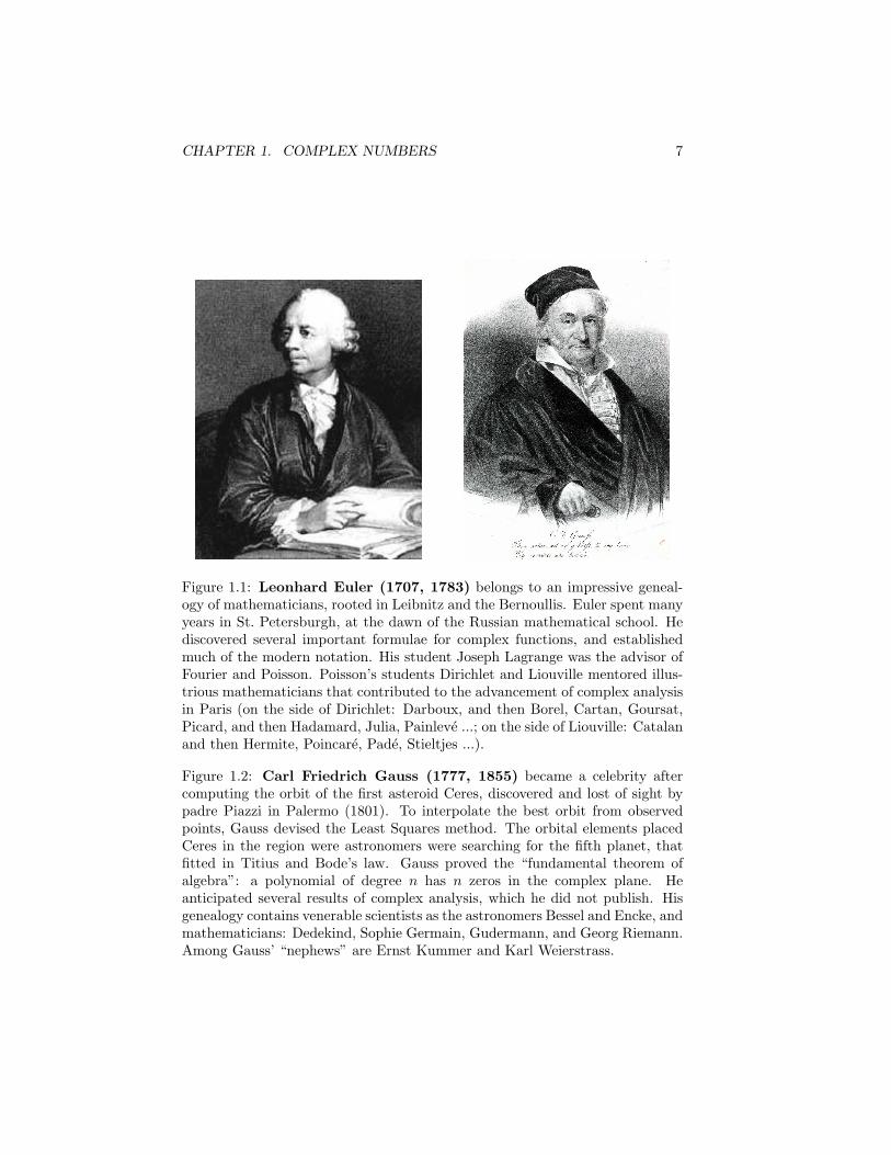
Figure 1.1: Leonhard Euler (1707, 1783) belongs to an impressive geneal-ogy of mathematicians, rooted in Leibnitz and the Bernoullis. Euler spent manyyears in St. Petersburgh, at the dawn of the Russian mathematical school. Hediscovered several important formulae for complex functions, and establishedmuch of the modern notation. His student Joseph Lagrange was the advisor ofFourier and Poisson. Poisson’s students Dirichlet and Liouville mentored illus-trious mathematicians that contributed to the advancement of complex analysisin Paris (on the side of Dirichlet: Darboux, and then Borel, Cartan, Goursat,Picard, and then Hadamard, Julia, Painleve ...; on the side of Liouville: Catalanand then Hermite, Poincare, Pade, Stieltjes ...).
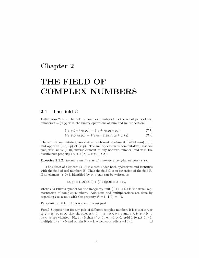
Figure 1.2: Carl Friedrich Gauss (1777, 1855) became a celebrity aftercomputing the orbit of the first asteroid Ceres, discovered and lost of sight bypadre Piazzi in Palermo (1801). To interpolate the best orbit from observedpoints, Gauss devised the Least Squares method. The orbital elements placedCeres in the region were astronomers were searching for the fifth planet, thatfitted in Titius and Bode’s law. Gauss proved the “fundamental theorem ofalgebra”: a polynomial of degree n has n zeros in the complex plane. Heanticipated several results of complex analysis, which he did not publish. Hisgenealogy contains venerable scientists as the astronomers Bessel and Encke, andmathematicians: Dedekind, Sophie Germain, Gudermann, and Georg Riemann.Among Gauss’ “nephews” are Ernst Kummer and Karl Weierstrass.
Chapter 2
THE FIELD OFCOMPLEX NUMBERS
2.1 The field CDefinition 2.1.1. The field of complex numbers C is the set of pairs of realnumbers z = (x, y) with the binary operations of sum and multiplication:
(x1, y1) + (x2, y2) = (x1 + x2, y1 + y2), (2.1)
(x1, y1)(x2, y2) = (x1x2 − y1y2, x1y2 + y1x2) (2.2)
The sum is commutative, associative, with neutral element (called zero) (0, 0)and opposite (−x,−y) of (x, y). The multiplication is commutative, associa-tive, with unity (1, 0), inverse element of any nonzero number, and with thedistributive property (z1 + z2)z3 = z1z3 + z2z3.
Exercise 2.1.2. Evaluate the inverse of a non-zero complex number (x, y).
The subset of elements (x, 0) is closed under both operations and identifieswith the field of real numbers R. Thus the field C is an extension of the field R.If an element (x, 0) is identified by x, a pair can be written as
(x, y) = (1, 0)(x, 0) + (0, 1)(y, 0) = x+ iy,
where i is Euler’s symbol for the imaginary unit (0, 1). This is the usual rep-resentation of complex numbers. Additions and multiplications are done byregarding i as a unit with the property i2 = (−1, 0) = −1.
Proposition 2.1.3. C is not an ordered field.
Proof. Suppose that for any pair of different complex numbers it is either z < wor z > w; we show that the rules a < b → a + c < b + c and a < b, c > 0 →ac < bc are violated. Fix i > 0 then i2 > 0 i.e. −1 > 0. Add 1 to get 0 > 1,multiply by i2 > 0 and obtain 0 > −1, which contradicts −1 > 0.
8
CHAPTER 2. THE FIELD OF COMPLEX NUMBERS 9
2.2 Complex conjugation
The complex conjugate (c.c.) of z = x+ iy is z = x− iy.Properties: z = z (c.c. is an involution), z1 + z2 = z1 + z2 and z1z2 = z1z2.The real numbers x and y are respectively the real and imaginary parts of z:
x = Re z =z + z
2, y = Im z =
z − z
2i.
2.3 Modulus
The modulus of a complex number is |z| =√x2 + y2. It is |z|2 = zz and
|z| = |z|, Re z ≤ |z| and Im z ≤ |z|. The following properties qualify themodulus as a norm and C as a normed space:
|z| ≥ 0, |z| = 0 iff z = 0, (2.3)
|z1z2| = |z1||z2|, (2.4)
|z1 + z2| ≤ |z1|+ |z2| (triangle inequality) (2.5)
Proof. The first is obvious. The second: use |z1z2|2 = z1z2z1z2. Triangleinequality: |z1 + z2|2 = (z1 + z2)(z1 + z2) = |z1|2 + |z2|2 + z1z2 + z1z2; the lasttwo terms are 2Re(z1z2) ≤ 2|z1z2| = 2|z1||z2|. Then |z1 + z2|2 ≤ |z1|2 + |z2|2 +2|z1||z2| = (|z1|+ |z2|)2.
If 1/z is the inverse of z it is |z(1/z)| = 1 i.e. |1/z| = 1/|z|.The modulus simplifies the evaluation of the inverse of a complex number:
1
z=
z
|z|2i.e.
1
x+ iy=
x
x2 + y2− i
y
x2 + y2
Remark 2.3.1. Property (2.4) has two interesting consequences:1) The unit circle |z| = 1 is closed for complex multiplication.2) For any four integers a, b, c, d there are integers p = ad+ bc and q = |ac− bd|such that (a2+b2)(c2+d2) = q2+p2. For example: (12+52)(12+72) = 122+342.
Exercise 2.3.2. Prove that |z1 + z2|2 + |z1 − z2|2 = 2|z1|2 + 2|z2|2 (in a paral-lelogram, the sum of the squares of the diagonals equals the sum of the squaresof the sides).
Exercise 2.3.3. Prove the very useful inequalities:
1√2(|x|+ |y|) ≤ |x+ iy| ≤ |x|+ |y| (2.6)∣∣∣ |z| − |w|
∣∣∣ ≤ |z − w| (2.7)
Hint: |z − w|2 = (|z| − |w|)2 + 2|z||w| − 2Re(zw).
2.4 Argument
A nonzero complex number z = x + iy may be represented as z = |z|(cos θ +i sin θ) (polar representation), where cos θ = x/|z| and sin θ = y/|z|. The number
CHAPTER 2. THE FIELD OF COMPLEX NUMBERS 10
cos θ + i sin θ belongs to the unit circle, where multiplication acts additively onphases:
(cos θ1 + i sin θ1)(cos θ2 + i sin θ2) = cos(θ1 + θ2) + i sin(θ1 + θ2).
De Moivre’s formula follows: (cos θ + i sin θ)n = cos(nθ) + i sin(nθ).At this stage, Euler’s representation cos θ + i sin θ = eiθ is introduced as a
definition. It is consistent with the rule eiθeiφ = ei(θ+φ). Then we write:
z = |z|(cos θ + i sin θ) = |z|eiθ (2.8)
The phase θ is the argument of z (θ = arg z) and is defined up to integermultiples of 2π. Note the property arg (z1z2) = arg z1 + arg z2.The principal argument Arg z is the single determination such that
−π < Arg z ≤ π.
With the choice −π2 < Arctan s ≤ π
2 , the geometric construction in fig.2.1 showsthat
Arg z = 2Arctany
|z|+ x(2.9)
The sign of Arg z is the same as y = Im z. The real negative semi-axis is a lineof discontinuity (branch cut). By definition its points have Arg z = π.
Z
ΘΘ2
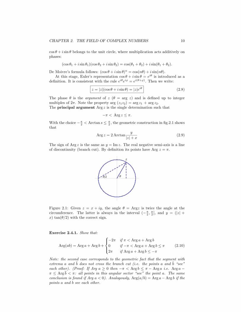
Figure 2.1: Given z = x + iy, the angle θ = Argz is twice the angle at thecircumference. The latter is always in the interval (−π
2 ,π2 ], and y = (|z| +
x) tan(θ/2) with the correct sign.
Exercise 2.4.1. Show that:
Arg(ab) = Arg a+Arg b+
−2π if π < Arg a+Arg b
0 if −π < Arg a+Arg b ≤ π
2π if Arg a+Arg b ≤ −π(2.10)
Note: the second case corresponds to the geometric fact that the segment withextrema a and b does not cross the branch cut (i.e. the points a and b “see”each other). (Proof: If Arg a ≥ 0 then −π < Arg b ≤ π − Arg a i.e. Arg a −π ≤ Arg b < π: all points in this angular sector “see” the point a. The sameconclusion is found if Arg a < 0). Analogously, Arg(a/b) = Arg a−Arg b if thepoints a and b see each other.
CHAPTER 2. THE FIELD OF COMPLEX NUMBERS 11
Other single determinations of the argument are possible, always having aline of discontinuity from the origin to infinity.For example, if the line is chosen as the imaginary half line z = ix (x ≥ 0), therange of values of this arg is (−3
2π,12π]. The points on the cut, by definition,
have argument 12π; other values are: arg(−1 + i) = −5π
4 , arg (−1) = −π, arg1 = 0.
Exercise 2.4.2. Write the numbers 1± i in polar form.
Exercise 2.4.3. Write eia + eib in polar form (a, b ∈ R). Answer: eia + eib =
2∣∣cos a−b
2
∣∣ e i2 (a+b)+iω, where ω = 0 or π if cos a−b
2 is positive or negative.
Exercise 2.4.4. Show that the numbers
z =1 + is
1− is, s ∈ R
belong to the unit circle. Is the map s→ Arg z invertible? If H is a Hermitianmatrix, show that U = (1 + iH)(1− iH)−1 is a unitary matrix.
2.5 Exponential
The exponential of a complex number z = x+ iy is defined as follows:
ez = exeiy = ex(cos y + i sin y) (2.11)
It exists for all z and defines the exponential function on C, with the fundamentalproperty
ezeζ = ez+ζ
The exponential function is periodic, with period 2πi: ez+2πi = ez, for all z.The trigonometric functions
cos z = 12 (e
iz + e−iz), sin z = 12i (e
iz − e−iz)
are periodic with period 2π, and (cos z)2 + (sin z)2 = 1. Note that they areunbounded in the imaginary direction. One also defines tan z = sin z/ cos z andcot z = 1/ tan z. The hyperbolic functions
cosh z = 12 (e
z + e−z), sinh z = 12 (e
z − e−z)
are periodic with period 2πi, and (cosh z)2−(sinh z)2 = 1. They are unboundedin the real direction. One defines tanh z = sinh z/ cosh z and coth z = 1/ tanh z.
Exercise 2.5.1.1) Show that |ez| = ex, ez = ez.2) Find the zeros of sinh(az + b), a, b ∈ R.3) Show that | cosh(x+ iy)| ≤ coshx.
Exercise 2.5.2 (Chebyshev polynomials).Show that cos(nθ) = Tn(t) is a polynomial in t = cos θ of degree n (Chebyshev
CHAPTER 2. THE FIELD OF COMPLEX NUMBERS 12
polynomial of the first kind). Evaluate the first few polynomials. Show that theyhave the following properties of recursion and orthogonality:
Tn+1(t)− 2t Tn(t) + Tn−1(t) = 0 (2.12)∫ 1
−1
dt√1− t2
Tm(t)Tn(t) =
0 n = m
π n = m = 0
π/2 n = m = 0
(2.13)
Prove similar properties for the Chebyshev polynomials of the second kind:
Un(t) =sin[(n+ 1)θ]
sin θ(t = cos θ).
Hint: 2 cos(nθ) = (cos θ + i sin θ)n + c.c.
2.6 Logarithm
The logarithm of a complex number z is the exponent that solves the equalityelog z = z. Note that log z is not defined in z = 0. Because of the periodicityof the exponential function, there are an infinite number of solutions: if log z isa solution, also log z + i2kπ is a solution for any integer k. All such solutionsare denoted as log z. The product rule of exponentials implies log(z1z2) =log z1 + log z2. In particular, with z = |z|eiθ one obtains
log z = log |z|+ i arg z + i 2kπ, k ∈ Z (2.14)
While the real part of log z is well determined as the log of a positive realnumber, the imaginary part reflects the same indeterminacy of the argument ofa complex number.It is natural to define the principal logarithm of a number as
Log z = log |z|+ iArg z (2.15)
The Log has a cut of discontinuity along the real negative axis: for vanishingϵ > 0 and x < 0: Log (x + iϵ) = log |x| + iπ (the formula holds also for ϵ = 0,Log (−1) = iπ) and Log (x− iϵ) = log |x| − iπ.
Remark 2.6.1. By ex.2.4.1, it is Log(ab) = Log a+Log b when a and b are insight; it is Log(a/b) = Log a− Log b when a and b are in sight.
In full analogy with the argument, different single-valued determinations ofthe log are possible and always have a line of discontinuity (branch cut) from0 to ∞ (branch points). Therefore, log(−i) is −iπ2 if the principal log (Log) isused. It is i 3π2 if the log is chosen with cut on the real positive half-line. It is−iπ2 if the cut is on the half-line z = ix, x ≥ 0.
Exercise 2.6.2. Evaluate Log 1+i1−i , Log(ie
iθ).
Exercise 2.6.3. What are Log(−z), Log z, Log(1/z), and Log(1/z) in termsof Log z?
Exercise 2.6.4. Prove that, for 0 < θ < π2 : Log (1 − eiθ) = log[2 sin( 12θ)] +
i 12 (θ − π).
CHAPTER 2. THE FIELD OF COMPLEX NUMBERS 13
2.7 Real powers
The real power of a complex number is defined as
za = ea log z (2.16)
In general it is multi-valued (such is the log):
za = |z|a exp (i a argz + i 2πak), k = 0,±1,±2, . . . (2.17)
Let’s consider the various cases:
• a ∈ Z: the power z±n is single-valued (z2 = z · z, z−1 = 1/z, etc.).
• a ∈ Q (a = ±p/q, with p and q coprime): the sequence of powers isperiodic, and only q roots are distinct.Example: (1 + i)2/3 = (
√2eiπ/4)2/3 = 21/3 exp(iπ6 + i43kπ), the values
k = 0, 1, 2 give three distinct powers.
• a is irrational: the set of powers is infinite.Example: (1+i)π = (
√2eiπ/4)π = 2π/2 exp(iπ2/4+i2π2k), k = 0,±1,±2, . . ..
Exercise 2.7.1. Evaluate: 81/3, (−1)1/5, i1/4, (1− i)1/6.
Exercise 2.7.2. Show that the square roots of z = a+ ib are:
±
√√a2 + b2 + a
2+ i
b
2
√2√
a2 + b2 + a
Exercise 2.7.3. Show the properties: |za| = |z|a, zazb = za+b, (zζ)a = zaζa
(for multivalued powers, the sets in the two sides must coincide).
Remark 2.7.4. Eq.(2.16) defines in general the power of a complex numberwith complex exponent:
za+ib = e(a+ib) log z
Examples: 1i = ei log 1 = ei(0+2πik)k∈Z = 1, e±2π, e±4π, . . . ;(1 + i)1−i = e(1−i)(log
√2+iπ
4 +2πik)k∈Z = √2eπ(
14+2k)ei(
π4 +2πk−log
√2)k∈Z
2.8 The fundamental theorem of algebra.
Among the great advantages of the complex field is the property that any poly-nomial of degree n with complex coefficients has precisely n zeros in C (funda-mental theorem of algebra)1. Therefore, a polynomial always admits the uniquefactorization:
p(z) = a0(z − z1)(z − z2) · · · (z − zn), (2.18)
1This intuitive explanation is from Timothy Gowers, The Princeton companion to Mathe-matics, Princeton University Press, (2009). Let p(z) = zn + a1zn−1 + · · ·+ an, with an = 0.For very large R the set p(Reiθ) ≈ Rneinθ, θ ∈ [0, 2π), approximates a circle of radius Rn
run n times, that contains the origin. For very small R, the set p(Reiθ) ≈ an−1Reiθ + an isa circle does not contain the origin. By continuity, there must be a value R such that the setcontains the origin i.e. an angle θ such that p(Reiθ) = 0.
CHAPTER 2. THE FIELD OF COMPLEX NUMBERS 14
where z1, . . . , zn are the zeros (or roots). The proof was provided by theprinceps mathematicorum Carl Friedrich Gauss, in his doctorate dissertationDemonstratio nova theorematis omnem functionem algebraicam rationalem in-tegram unius variabilis in factores reales primi vel secundi gradus resolvi posse(1799). Through graphical methods he showed that any polynomial p(x+ iy) =u(x, y) + iv(x, y) (with real coefficients) necessarily has at least one root. Theequations u(x, y) = 0 and v(x, y) = 0 describe two curves in the plane, andGauss was able to show that they have at least one intersection. Before him,Girard (1629), d’Alembert (1748) and Euler (1749), proved the weaker state-ment that any polynomial with real coefficients can be factorized into real linearand quadratic terms.A simple rigorous proof of the fundamental theorem will be given on the basisof Liouville’s theorem for entire functions.
2.9 The cyclotomic equation
The roots of the equation zn = 1 are the corners of a regular n-polygon inscribedin the unit circle:
ζk = cos2kπ
n+ i sin
2kπ
n, k = 0, . . . , n− 1.
Since zn − 1 = (z − 1)(zn−1 + · · · + z + 1), the roots ζ1, . . . , ζn−1 solve thecyclotomic equation zn−1 + · · ·+ z + 1 = 0.In 1796 Gauss, then a young student, announced the possibility to construct byruler and compass the regular polygon with n = 17 sides. Five years later hegave a sufficient condition2 for a polygon to be constructible by ruler and com-pass: n = 2k pm1
1 pm22 · · · , where the factor 2k accounts for repeated duplications
of the number of sides of a more basic polygon. The powers pm are either 1 orpowers of a Fermat number (i.e. p = 22
q
+1) that is also a prime number3. Thepolygons n = 3, 4, 5 (i.e. p = 1, 3, 5) and duplications (n = 6, 8, 10, 12, . . . ) were
known since Euclid’s time. The next Fermat prime number is p = 222
+1 = 17.Gauss was so proud of his discovery, that he asked for a 17-polygon to be carvedon his gravestone4.
Exercise 2.9.1. Let ζkn−1k=0 be the roots of zn = 1. Show that:
ζp0 + · · ·+ ζpn−1 = 0 p = 1, . . . , n− 1 (2.19)
an − bn = (a− b)(a− ζ1b) · · · (a− ζn−1b) (2.20)
Exercise 2.9.2. Consider the polygon with corners at the n roots of unity1, ζ, . . . , ζn−1 and draw the diagonals connecting 1 to the other corners. Showthat the product of their lengths is precisely n: |1 − ζ| · · · |1 − ζn−1| = n (anamusing generalization to the ellipse is discussed in arXiv:1810.00492).
Exercise 2.9.3. Solve the equation z5 = 1 for the vertices of a pentagon, andobtain cos 2π
5 = 14 (√5 − 1). (Hint: let ζk = ei2πk/5, k = 0, .., 4 be the solutions.
2Wantzel (1836) showed that it is also necessary.3Euler showed that the Fermat number 232 + 1 (q = 5) is not a prime number.4The tale of the (28 + 1)−gon is narrated in the nice book Dr. Euler’s fabulous formula
by Paul Nahin, Princeton Univ. Press (2006).
CHAPTER 2. THE FIELD OF COMPLEX NUMBERS 15
Since their sum is zero (the coefficient of z4 is zero in the equation), also the real part
of the sum vanishes: 1 + 2 cos 2π5
+ 2 cos 4π5
= 0, whereby the solution is found.)
Exercise 2.9.4 (Discrete Fourier transform5). Show that the following N ×Nmatrix
Frs =1√Nei
2πN rs
is unitary. Evaluate F 2 and show that F 4 = 1. What are the eigenvalues of F?(Hint: you need the sum of powers of the N roots of unity).
Exercise 2.9.5 (Madhava Math. competition, 2013). Let ζ1, . . . ζN be the Nroots of unity. Show that if z is a point of the unit circle, then the sum ofsquared distances
∑Nk=1 |z − ζk|2 is the same for all z.
Exercise 2.9.6. Consider the following n× n matrix:
S =
0 1
. . .. . .
. . . 11 0
(2.21)
Its action on a vector u ∈ Cn is a cyclic shift of the components: (Su)k = uk+1
and (Su)n = u1. Therefore Sn = In.1) Show that Sn−1 = ST (T means transposition).2) Find the eigenvalues and the eigenvectors of S.3) Find the spectrum of the periodic “Laplacian matrix” ∆ = S + ST − 2In
∆ =
−2 1 1
1. . .
. . .
. . .. . . 1
1 1 −2
4) Find the characteristic poylnomial det(zIn −∆).5) Write down the circulant matrix a0 + a1S + · · · + an−1S
n−1, ai ∈ C, andevaluate its eigenvalues and eigenvectors.
Exercise 2.9.7. Evaluate the characteristic polynomial of the n× n matrix
H0 =
0 1 0
1. . .
. . .
. . .. . . 1
0 1 0
.Hint: Let Dk(z) = det[zIk −H0]; show that Dk+1(z) − zDk(z) +Dk−1(z) = 0. Notethat: [
Dk+1(z)Dk(z)
]= T k
[D1(z)D0(z)
], T =
[z −11 0
]T k is the “transfer matrix”, and D1(z) and D0(z) are the initial conditions. By the
Cayley-Hamilton theorem, T 2 − zT + I2 = 0. This implies T k = akT + bkI2 with
numbers ak, bk to be found.
5M.L.Mehta, Eigenvalues and eigenvectors of the finite Fourier transform, J. Math. Phys.28 (1987) 781.
Chapter 3
THE COMPLEX PLANE
The modulus of a complex number defines an Euclidean distance between pointsz = (x, y) and z′ = (x′, y′) in the complex plane:
d(z, z′) = |z − z′| =√(x− x′)2 + (y − y′)2 (3.1)
Results of Cartesian geometry of R2 can be transposed to C. Disks, circles andlines are important in complex analysis; let’s review them in complex notation.
3.1 Straight lines and circles
Given two points a and b in C, the oriented straight line ab has parametricequation z(t) = (1− t)a+ tb, t ∈ R. The restriction 0 ≤ t ≤ 1 traces the closedsegment [a, b] from a to b.A circle C(a, r) with center a and radius r has equation |z − a| = r. Theparameterization
z(θ) = a+ reiθ, 0 ≤ θ < 2π (3.2)
endows the circle with the standard anticlockwise orientation.
Exercise 3.1.1.1) Give conditions for the lines ab and cd to be parallel or orthogonal.2) Find the corners of the squares and of the equilateral triangles having oneside on the segment [a, b].3) Describe the sets: Arg(z − i) = π
3 , |Arg(z − i)| < π3 .
4) Given three points z1, z2, z3, find the circle through them.5) Show that the locus |z − a|2 + |z − b|2 = |a − b|2 is a circle with diameter[a, b]. Find the parametric equation of the circle.6) Show that the locus |z − a| = λ|z − b|, λ > 0, is a circle with radius r =
λ|1−λ2| |a − b| and center c = a−λ2b
1−λ2 . The value λ = 1 corresponds to the limit
case of a line (the axis of the segment [a, b]).
Exercise 3.1.2.1) Find the equation of the ellipse with foci z1 and z2, major semiaxis length a.
16
CHAPTER 3. THE COMPLEX PLANE 17
2) Study the family of Cassini ovals1 |z2 − 1| = r2 as r changes. Show that it isa single closed line for r ≥ 1.3) Give the conditions for a point z to be inside the triangle with vertices a, b, c.Answer: z = αa+ βb+ γc, where α+ β + γ = 1 and 0 ≤ α, β, γ ≤ 1.
3.2 Simple maps
In this section we study simple maps w = F (z), where F : C → C. The subjectis of considerable interest and will be fully appreciated after the discussion ofanalytic functions.It is useful to introduce the extended complex plane C by adjoining thepoint ∞ to C with the rules z +∞ = ∞+ z = ∞ and z∞ = ∞z = ∞ (z = 0).Moreover, one puts the conventions z/∞ = 0 (z = ∞), and z/0 = ∞ (z = 0).
3.2.1 The linear map
The linear map w = az + b has one fixed point2 z⋆ = b/(1 − a). By writingw − z⋆ = a(z − z⋆) one obtains
|w − z⋆| = |a||z − z⋆|, arg (w − z⋆) = arg a+ arg (z − z⋆)
Therefore the map is a dilation by a factor |a| of all segments originating fromz⋆ and a rotation of the plane by arg a around the fixed point.Equivalently, the map can be viewed as a rotation by arg a around the originand a dilation centred in the origin (z′ = az), followed by a shift (w = z′ + b).
Exercise 3.2.1. Show that a linear map takes circles to circles and straightlines to straight lines.
3.2.2 The inversion map
The map w = 1/z transforms a circle |z| = r centred in the origin into the circle|w| = 1/r. The interior of the unit circle is exchanged with the exterior.By regarding straight lines as circles with a point at infinity, the inversion takescircles to circles (prove it). Then, a straight line that does not contain the originis mapped to a circle through the origin; only straight lines through the origin(containing both 0 and ∞) are mapped to straight lines through the origin.Conversely, circles through the origin are mapped to straight lines, and circlesnot through the origin are mapped to circles.Set w = u+ iv, the image of x+ iy has Cartesian coordinates
u =x
x2 + y2, v = − y
x2 + y2
A line u(x, y) = U in w−plane is the image of a circle through the origin z = 0with center ( 1
2U , 0). A line v(x, y) = V is the image of a circle again through theorigin with center (0,− 1
2V ). All these circles, that are mapped to the orthogonalgrid of u − v lines, are orthogonal to each other (we’ll give a general proof ofthis).
1A Cassini oval is the planar locus of points whose distances from two points have constantproduct: |z − a| · |z − b| = C2.
2A fixed point of a map is one that is mapped in itself, z⋆ = F (z⋆).
CHAPTER 3. THE COMPLEX PLANE 18
x
y
−6
4v=−1/4
u=−1/6u=1/3
v=1/2
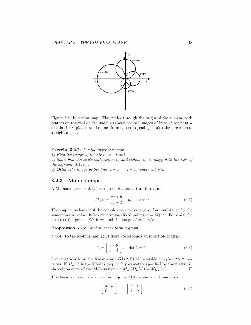
Figure 3.1: Inversion map. The circles through the origin of the z plane withcenters on the real or the imaginary axis are pre-images of lines of constant uor v in the w plane. As the lines form an orthogonal grid, also the circles crossat right angles.
Exercise 3.2.2. For the inversion map:1) Find the image of the circle |z − i| = 1.2) Show that the circle with center z0 and radius |z0| is mapped to the axis ofthe segment [0, 1/z0].3) Obtain the image of the line |z − a| = |z − b|, where a, b ∈ C.
3.2.3 Mobius maps
A Mobius map w =M(z) is a linear fractional transformation
M(z) =az + b
cz + d, ad− bc = 0 (3.3)
The map is unchanged if the complex parameters a, b, c, d are multiplied by thesame nonzero value. It has at most two fixed points z⋆ =M(z⋆). For c = 0 theimage of the point −d/c is ∞, and the image of ∞ is a/c.
Proposition 3.2.3. Mobius maps form a group.
Proof. To the Mobius map (3.3) there corresponds an invertible matrix
L =
[a bc d
], detL = 0. (3.4)
Such matrices form the linear group GL(2,C) of invertible complex 2 × 2 ma-trices. If ML(z) is the Mobius map with parameters specified by the matrix L,the composition of two Mobius maps is ML′(ML(z)) =ML′L(z).
The linear map and the inversion map are Mobius maps with matrices[a b0 1
] [0 11 0
](3.5)
CHAPTER 3. THE COMPLEX PLANE 19
If c = 0 the factorization[a bc d
]=
[−ad−bc
cac
0 1
] [0 11 0
] [c d0 1
]. (3.6)
shows that a Mobius map is a composition of two linear maps with an inversionbetween (the case c = 0 is already a linear map). As a consequence:1) circles are mapped to circles (where a straight line is a circle with point at∞). More precisely, M(z) takes every line and circle passing through −d/c intoa line, and every other line or circle into a circle.2) Mobius maps are bijections from C to C (actually, they are the most generalbijections of the extended complex plane).
Example 3.2.4. Show that the Mobius maps of the upper half-plane H = z :Imz > 0 to the unit disk D = w : |w| < 1, are
w = eiϑz − z0z − z0
(3.7)
where z0 is the point with Im z0 > 0 that is mapped to w = 0 (the center) andthe prefactor is a rotation of the disk.
Proof. Let w(z) have the form (3.3), with c = 1. Since a boundary is mapped toa boundary, the image of the real axis must be the unit circle. Then |ax+ b| =|x+ d| for all real x. The limit cases x → ∞ and x = 0 imply |a| = 1, |b| = |d|i.e. a = eiϑ, b = −eiϑz0, |d| = |z0|. Then |x − z0| = |x − d| for all x i.e.:x2+ |z0|2−2xRe z0 = x2+ |z0|2−2xRe d. The equation is solved by d = z0.
A Mobius map can be specified by requiring that three points (z1, z2, z3) aremapped (in the order) to prescribed points (w1, w2, w3). The choice (0, 1,∞)for the image points gives the Mobius map
M(z) =z − z1z − z3
z2 − z3z2 − z1
. (3.8)
It maps the circle through z1, z2 and z3 to the real axis (the circle that contains0,1 and ∞).
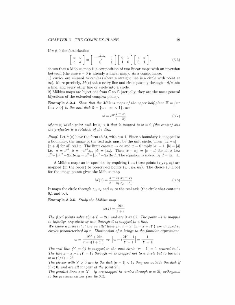
Example 3.2.5. Study the Mobius map
w(z) =2iz
z + i
The fixed points solve z(z + i) = 2iz and are 0 and i. The point −i is mappedto infinity: any circle or line through it is mapped to a line.We know a priori that the parallel lines Im z = Y (z = x+ iY ) are mapped tocircles parameterized by x. Elimination of x brings to the familiar expression:
w =−2Y + 2ix
x+ i(1 + Y )⇒∣∣∣w − i
2Y + 1
Y + 1
∣∣∣ = 1
|Y + 1|The real line (Y = 0) is mapped to the unit circle |w − 1| = 1 centred in 1.The line z = x− i (Y = 1) through −i is mapped not to a circle but to the linew = (2/x) + 2i.The circles with Y > 0 are in the disk |w − 1| < 1; they are outside the disk ifY < 0, and are all tangent at the point 2i.The parallel lines z = X + iy are mapped to circles through w = 2i, orthogonalto the previous circles (see fig.3.2).
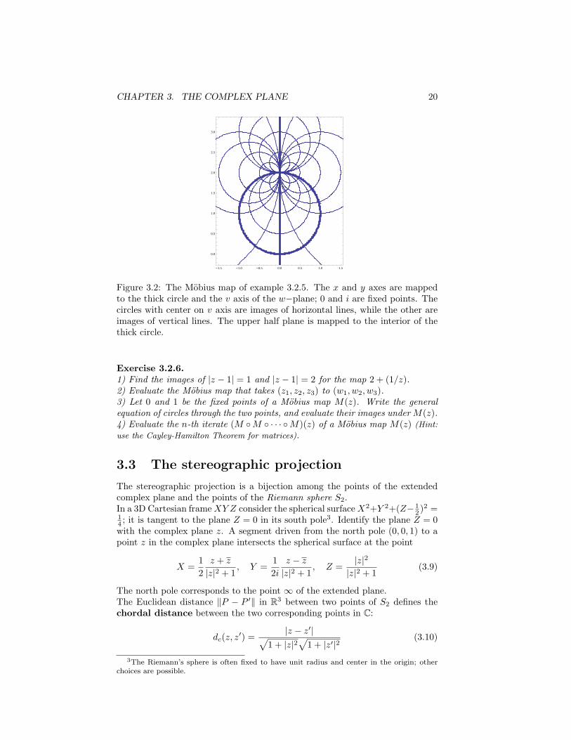
CHAPTER 3. THE COMPLEX PLANE 20
-1.5 -1.0 -0.5 0.0 0.5 1.0 1.5
0.0
0.5
1.0
1.5
2.0
2.5
3.0
Figure 3.2: The Mobius map of example 3.2.5. The x and y axes are mappedto the thick circle and the v axis of the w−plane; 0 and i are fixed points. Thecircles with center on v axis are images of horizontal lines, while the other areimages of vertical lines. The upper half plane is mapped to the interior of thethick circle.
Exercise 3.2.6.1) Find the images of |z − 1| = 1 and |z − 1| = 2 for the map 2 + (1/z).2) Evaluate the Mobius map that takes (z1, z2, z3) to (w1, w2, w3).3) Let 0 and 1 be the fixed points of a Mobius map M(z). Write the generalequation of circles through the two points, and evaluate their images underM(z).4) Evaluate the n-th iterate (M M · · · M)(z) of a Mobius map M(z) (Hint:
use the Cayley-Hamilton Theorem for matrices).
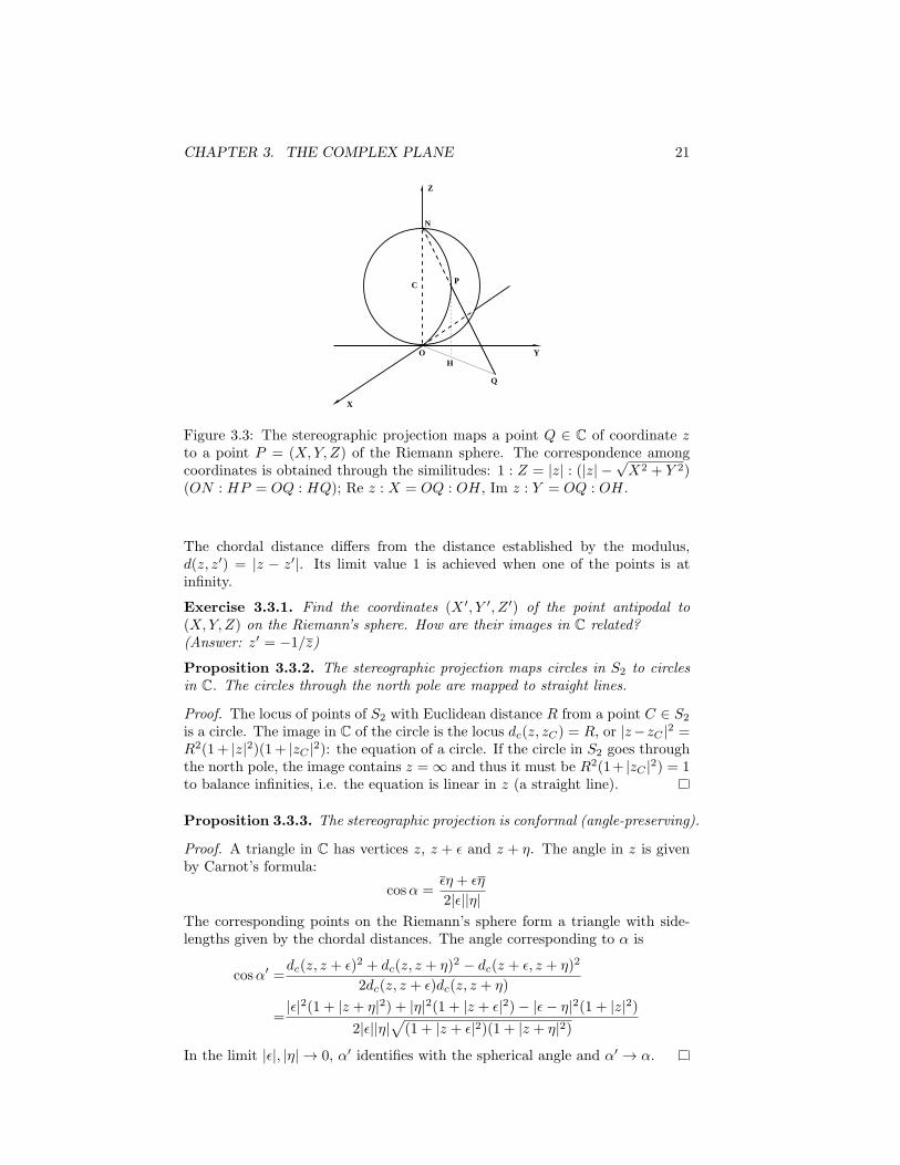
3.3 The stereographic projection
The stereographic projection is a bijection among the points of the extendedcomplex plane and the points of the Riemann sphere S2.In a 3D Cartesian frameXY Z consider the spherical surfaceX2+Y 2+(Z− 1
2 )2 =
14 ; it is tangent to the plane Z = 0 in its south pole3. Identify the plane Z = 0with the complex plane z. A segment driven from the north pole (0, 0, 1) to apoint z in the complex plane intersects the spherical surface at the point
X =1
2
z + z
|z|2 + 1, Y =
1
2i
z − z
|z|2 + 1, Z =
|z|2
|z|2 + 1(3.9)
The north pole corresponds to the point ∞ of the extended plane.The Euclidean distance ∥P − P ′∥ in R3 between two points of S2 defines thechordal distance between the two corresponding points in C:
dc(z, z′) =
|z − z′|√1 + |z|2
√1 + |z′|2
(3.10)
3The Riemann’s sphere is often fixed to have unit radius and center in the origin; otherchoices are possible.
CHAPTER 3. THE COMPLEX PLANE 21
Y
Z
P
N
OH
Q
X
C
Figure 3.3: The stereographic projection maps a point Q ∈ C of coordinate zto a point P = (X,Y, Z) of the Riemann sphere. The correspondence amongcoordinates is obtained through the similitudes: 1 : Z = |z| : (|z| −
√X2 + Y 2)
(ON : HP = OQ : HQ); Re z : X = OQ : OH, Im z : Y = OQ : OH.
The chordal distance differs from the distance established by the modulus,d(z, z′) = |z − z′|. Its limit value 1 is achieved when one of the points is atinfinity.
Exercise 3.3.1. Find the coordinates (X ′, Y ′, Z ′) of the point antipodal to(X,Y, Z) on the Riemann’s sphere. How are their images in C related?(Answer: z′ = −1/z)
Proposition 3.3.2. The stereographic projection maps circles in S2 to circlesin C. The circles through the north pole are mapped to straight lines.
Proof. The locus of points of S2 with Euclidean distance R from a point C ∈ S2
is a circle. The image in C of the circle is the locus dc(z, zC) = R, or |z−zC |2 =R2(1+ |z|2)(1+ |zC |2): the equation of a circle. If the circle in S2 goes throughthe north pole, the image contains z = ∞ and thus it must be R2(1+ |zC |2) = 1to balance infinities, i.e. the equation is linear in z (a straight line).
Proposition 3.3.3. The stereographic projection is conformal (angle-preserving).
Proof. A triangle in C has vertices z, z + ϵ and z + η. The angle in z is givenby Carnot’s formula:
cosα =ϵη + ϵη
2|ϵ||η|The corresponding points on the Riemann’s sphere form a triangle with side-lengths given by the chordal distances. The angle corresponding to α is
cosα′ =dc(z, z + ϵ)2 + dc(z, z + η)2 − dc(z + ϵ, z + η)2
2dc(z, z + ϵ)dc(z, z + η)
=|ϵ|2(1 + |z + η|2) + |η|2(1 + |z + ϵ|2)− |ϵ− η|2(1 + |z|2)
2|ϵ||η|√
(1 + |z + ϵ|2)(1 + |z + η|2)
In the limit |ϵ|, |η| → 0, α′ identifies with the spherical angle and α′ → α.
CHAPTER 3. THE COMPLEX PLANE 22
Exercise 3.3.4 (Rotations). Show that the Mobius maps that preserve thechordal distance, dc(M(z),M(z′)) = dc(z, z
′) for all z, z′ ∈ C, have
|a|2 + |c|2 = |b|2 + |d|2 = 1, ab+ cd = 0, |ad− bc| = 1
They form a group, which is represented by the matrix group U(2) of unitarymatrices on C2. Via the stereographic map, these maps induce rigid transfor-mations of the sphere S2 to itself (rotations and reflections).The subgroup SU(2) corresponds to ad− bc = 1, and induces pure rotations.
Chapter 4
SEQUENCES ANDSERIES
4.1 Topology
The modulus endows C with the structure of normed space1 and defines a dis-tance between points, d(z, z′) = |z− z′|. Therefore (C, d) is also a metric space.Furthermore, at every point z one may introduce a basis of neighbourhoods,which makes C a topological space. The elements of the basis are the diskscentred in z with radii r > 0:
D(z, r) = ζ : |ζ − z| < r.
The following definitions and statements are important and used thoroughly:
• A set S in C is open if for every point z ∈ S there is a diskD(z, r) wholly inS. The union of any collection of open sets is an open set; the intersectionof two open sets is open.
• A point z ∈ C is an accumulation point of a set S if every disk D(z, r)contains a point in S different from z.
• A boundary point of S is a point z such that every disk D(z, r) containspoints in S and points not in S. The boundary of S is the set ∂S ofboundary points of S.
• A set is closed if it contains all its boundary points. The closure of a setS is the set S = S ∪ ∂S.
• A set S is disconnected if there are two disjoint open sets A and B suchthat S ⊆ A ∪B but S is not a subset of A or B alone. A set is connectedif it is not disconnected.
Proposition 4.1.1. A set S is closed if and only if C/S is open.
1Normed, metric and topological spaces are general structures that will be defined later.
23
CHAPTER 4. SEQUENCES AND SERIES 24
Proof. Suppose that S is closed, then for any z /∈ S there is a disk that doesnot contain points in S (otherwise z ∈ ∂S ⊂ S), i.e. C/S is open. On the otherhand, if C/S is open, every point in C/S cannot be in ∂S, i.e. S contains itsfrontier (S is closed).
Definition 4.1.2. A domain is a set both open and connected.
Proposition 4.1.3. Any two points in a domain can be joined by a continuouspolygonal line in the domain.
4.2 Sequences
Complex sequences are maps N → C, and are basic objects in mathematics.They arise in analysis, approximation theory, iteration of maps. Infinite seriesand infinite products are limits of sequences of partial sums and partial products.General statements about sequences are now presented.
Definition 4.2.1. A sequence zn converges to z (zn → z) if |zn − z| → 0 i.e.
∀ϵ ∃Nϵ such that |zn − z| < ϵ, ∀n > Nϵ. (4.1)
Exercise 4.2.2. Show that:1) if zn → z and wn → w then: i) zn + wn → z + w, ii) znwn → zw, iii)zn/wn → z/w if wn, w = 0, iv) zn → z.2) a sequence zn is convergent if and only if both Re zn and Im zn are convergentin R.3) if zn → z, then |zn| → |z|. Hint: use inequality (2.7).
Definition 4.2.3. A sequence zn is a Cauchy sequence if
∀ϵ > 0 ∃Nϵ such that : |zn − zm| < ϵ, ∀m,n > Nϵ. (4.2)
A convergent sequence is always a Cauchy sequence, but the converse may notbe true. When every Cauchy sequence is convergent to a limit in the space, thespace is termed complete. The Cauchy criterion is then an extremely useful toolto predict convergence, without the need to identify the limit.
Proposition 4.2.4. C is complete
Proof. The inequalities (2.6) imply that xn+ iyn is a Cauchy sequence if andonly if both xn and yn are Cauchy sequences. Since R is complete, theyboth converge. Let x and y be their limits, then |(xn+ iyn)− (x+ iy)| → 0.
4.2.1 Quadratic maps, Julia and Mandelbrot sets
The iteration of a map z′ = F (z), with function F : C → C and initial valuez, generates a sequence: z, F (z), F (F (z)), ... A sequence depends on theinitial value, and this dependence may be surprisingly interesting. The problemwas studied by Pierre Fatou and Gaston Julia in the early 1900. The simplestnon-trivial function is
F (z) = z2 + c, c ∈ C.
CHAPTER 4. SEQUENCES AND SERIES 25
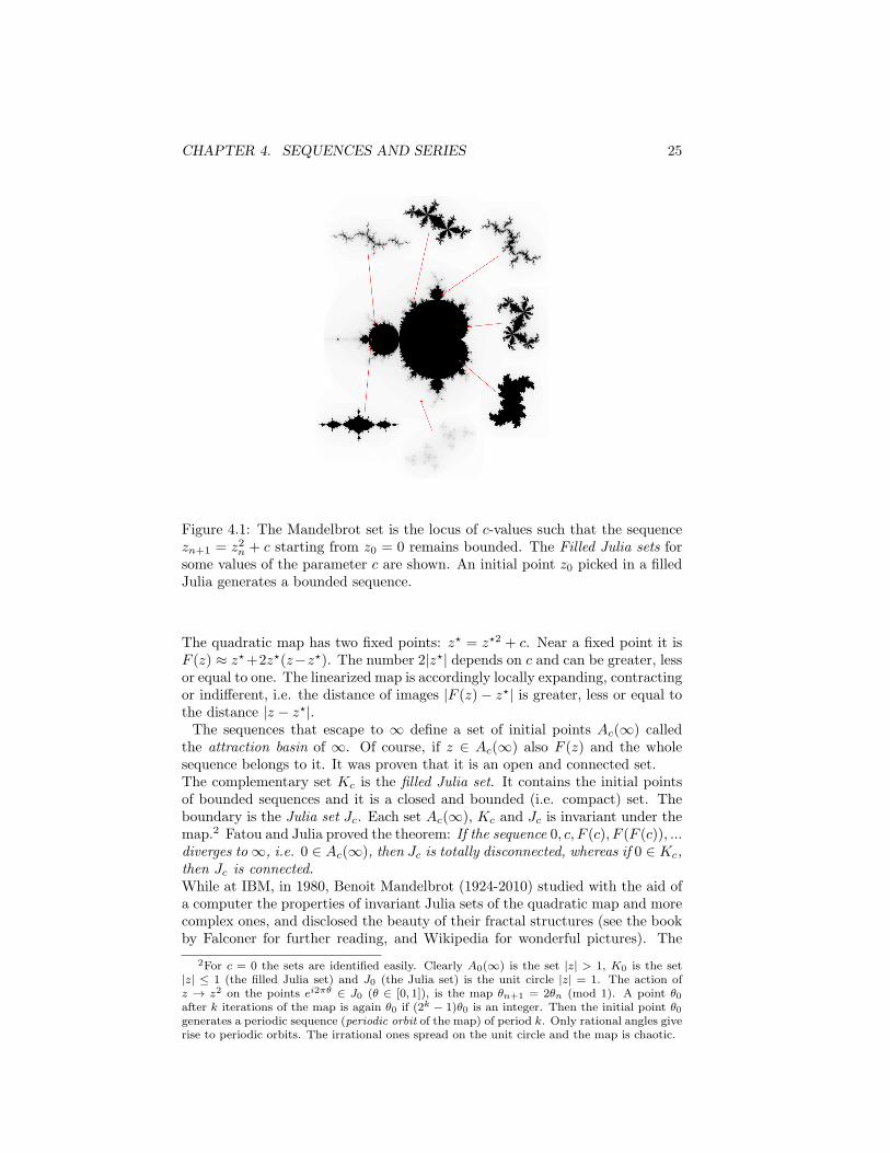
Figure 4.1: The Mandelbrot set is the locus of c-values such that the sequencezn+1 = z2n + c starting from z0 = 0 remains bounded. The Filled Julia sets forsome values of the parameter c are shown. An initial point z0 picked in a filledJulia generates a bounded sequence.
The quadratic map has two fixed points: z⋆ = z⋆2 + c. Near a fixed point it isF (z) ≈ z⋆+2z⋆(z−z⋆). The number 2|z⋆| depends on c and can be greater, lessor equal to one. The linearized map is accordingly locally expanding, contractingor indifferent, i.e. the distance of images |F (z)− z⋆| is greater, less or equal tothe distance |z − z⋆|.The sequences that escape to ∞ define a set of initial points Ac(∞) called
the attraction basin of ∞. Of course, if z ∈ Ac(∞) also F (z) and the wholesequence belongs to it. It was proven that it is an open and connected set.The complementary set Kc is the filled Julia set. It contains the initial pointsof bounded sequences and it is a closed and bounded (i.e. compact) set. Theboundary is the Julia set Jc. Each set Ac(∞), Kc and Jc is invariant under themap.2 Fatou and Julia proved the theorem: If the sequence 0, c, F (c), F (F (c)), ...diverges to ∞, i.e. 0 ∈ Ac(∞), then Jc is totally disconnected, whereas if 0 ∈ Kc,then Jc is connected.While at IBM, in 1980, Benoit Mandelbrot (1924-2010) studied with the aid ofa computer the properties of invariant Julia sets of the quadratic map and morecomplex ones, and disclosed the beauty of their fractal structures (see the bookby Falconer for further reading, and Wikipedia for wonderful pictures). The
2For c = 0 the sets are identified easily. Clearly A0(∞) is the set |z| > 1, K0 is the set|z| ≤ 1 (the filled Julia set) and J0 (the Julia set) is the unit circle |z| = 1. The action ofz → z2 on the points ei2πθ ∈ J0 (θ ∈ [0, 1]), is the map θn+1 = 2θn (mod 1). A point θ0after k iterations of the map is again θ0 if (2k − 1)θ0 is an integer. Then the initial point θ0generates a periodic sequence (periodic orbit of the map) of period k. Only rational angles giverise to periodic orbits. The irrational ones spread on the unit circle and the map is chaotic.
CHAPTER 4. SEQUENCES AND SERIES 26
Mandelbrot set (1980) is the set of parameters c ∈ C such that Jc is connected.Again, it is a wonderful fractal3.
Exercise 4.2.5. Consider the linear map zn+1 = azn + b. Write the generalexpression of zn in terms of z0. When is the sequence bounded?
Exercise 4.2.6. Study the fixed points z⋆ of the exponential map z′ = ez.Show that they come in pairs x± iy with x > 0, |y| > 1 (then the linearized mapz′ = z⋆ + z⋆(z − z⋆) is locally expanding)4.
4.3 Series
Infinite sums were studied long before sequences. The oldest known series ex-pansions were obtained by Madhava (1350, 1425), the founder of the Keralaschool of astronomy and mathematics. He developed series for trigonometricfunctions, including an error term. The one for arctan x enabled him to eval-uate π up to 11 digits. His work may have influenced European mathematicsthrough transmission by the Jesuits. The same series were rediscovered by Gre-gory two centuries later.Oresme in the XIV century, Jakob & Johann Bernoulli (Tractatus de seriebusinfinitis, 1689), and Pietro Mengoli (1625, 1686), discovered and rediscoveredthe divergence of the Harmonic series 1+ 1
2 +13 + . . . In the Tractatus, the con-
vergence of∑
k 1/k2 was also proven, but the sum was evaluated later (1734) by
Johann’s prodigious student Leonhard Euler. Euler also proved that the sumof the reciprocals of prime numbers is divergent5.Christian Huygens asked his student Leibnitz to evaluate the sum of reciprocalsof triangular numbers6. The result (the sum is 2) was obtained after notingthat 1
k(k+1) =1k − 1
k+1 (the sum is a telescopic series).
Series gained rigour after Cauchy, who defined convergence in terms of the se-quence of partial sums.
Given a sequence of complex numbers ak one constructs the partial sumsAn =
∑nk=0 ak. If the sequence An converges to a finite limit A, the limit is the
sum of the series
A =∞∑k=0
ak.
If∑∞
k ak = A and∑∞
k bk = B, where A and B are finite, the series∑∞
k (ak±bk)is convergent and the sum is A±B.
Proposition 4.3.1. A necessary and sufficient condition for a series to con-
3The boundary is the “Mandelbrot lemniscate”. It is the limit of a sequence of level curves(lemniscates) Mn = z ∈ C : |pn(z)| = 2, where pn(z) is the sequence of polynomials:p1(z) = z, pn+1(z) = pn(z)2 + z.
4The map is chaotic, and is studied in arXiv:1408.1129.5For nice accounts see P. Pollack, Euler and the partial sums of the prime harmonic series,
http://alpha.math.uga.edu/ pollack/eulerprime.pdf; M.Villarino, Mertens Proof of MertensTheorem, arXiv:math/0504289.
6The triangular numbers are n1 = 1, nk+1 = nk + k = 1 + 2 + · · ·+ k =k(k+1)
2.
CHAPTER 4. SEQUENCES AND SERIES 27
verge is that the sequence of partial sums is a Cauchy sequence:
∀ϵ > 0 ∃Nϵ such that ∀m > Nϵ and ∀n > 0 :
∣∣∣∣∣m+n∑
k=m+1
ak
∣∣∣∣∣ < ϵ. (4.3)
In particular for n = 1 it is |am+1| < ϵ. Therefore a necessary condition forconvergence is |ak| → 0.
4.3.1 Absolute convergence
The inequality |∑m+n
m+1 ak| ≤∑m+n
m+1 |ak| implies that if∑∞
k=1 |ak| converges,then also
∑∞k=1 ak does.
Definition 4.3.2. A series∑
k ak is absolutely convergent if∑
k |ak| is conver-gent.
Absolute convergence is a sufficient criterion for convergence; moreover it dealswith series in R. We state but not prove the important property
Proposition 4.3.3. The sum of an absolutely convergent series does not changeif the terms of the series are permuted7:
∑k ak =
∑k aπ(k).
The following are sufficient conditions for absolute convergence of the series∑k ak. They must hold for k greater than some N :
• Comparison (Gauss):
|ak| < bk, where∑k
bk <∞
• Ratio (D’Alembert): for ak = 0
lim supk
|ak+1||ak|
< 1
• Root (Cauchy-Hadamard):
lim supk
k√|ak| < 1
Proposition 4.3.4 (Cesaro). If the sequences |ak|1/k and |ak+1||ak| converge to
finite limits, the limits are equal. The limit coincides with lim sup.
7A convergent series that is not absolutely convergent is conditionally convergent. Theseries
∑∞k=1 i
k/k is convergent as it is the sum of two convergent series∑
k≥1(−1)k/(2k) +
i∑
k≥0(−1)k/(2k+1), and is conditionally convergent. Riemann proved the surprising resultthat by rearranging terms of a conditionally convergent real series one can obtain any limitsum in R.
CHAPTER 4. SEQUENCES AND SERIES 28
4.3.2 Cauchy product of series
The Cauchy product of two series is the series of finite sums:[ ∞∑k=0
ak
][ ∞∑r=0
br
]=
∞∑k=0
(k∑
r=0
arbk−r
)(4.4)
Proposition 4.3.5 (Franz Mertens, 18748). If a series is absolutely convergentto A and another is convergent to B, their Cauchy product is convergent to AB.
Proposition 4.3.6. If a series is absolutely convergent to A and another isabsolutely convergent to B, their Cauchy product is absolutely convergent toAB.
Proof.
n∑k=0
|ck| =n∑
k=0
∣∣∣∣∣k∑
r=0
arbk−r
∣∣∣∣∣ ≤n∑
k=0
k∑r=0
|ar||bk−r|
=n∑
r=0
|ar|n∑
k=r
|bk−r| =n∑
r=0
|ar|n−r∑k=0
|bk| ≤∞∑k=0
|ak|∞∑l=0
|bl|
Since the sequence∑n
k=0 |ck| is non decreasing and bounded above, it is conver-gent. Then Ck =
∑nk=0 ck is absolutely convergent to a limit C. The limit does
not depend on rearrangements of terms and is the sum of all possible productsarbs. It can be evaluated as follows: C = limk(AkBk) = (limk Ak)(limk Bk) =AB.
4.3.3 The geometric series
The partial sums Sn = 1 + z + . . . + zn can be evaluated from the identitiesSn+1 = Sn + zn+1 and Sn+1 = 1 + zSn:
n∑k=0
zk =1− zn+1
1− z, z = 1 (4.5)
If |z| < 1, it is limn→∞ zn = 0 and Sn(z) converges to the simple but funda-mental geometric series
∞∑n=0
zn =1
1− z, |z| < 1 (4.6)
The geometric series is useful for assessing convergence of series by the com-parison test. Consider for example the Jacobi theta function (for simplicity, we
restrict to x ∈ R): ϑ3(x, q) = 1 + 2∑∞
m=1 qm2
cos(2mx), |q| < 1. The series isabsolutely convergent:
|ϑ3(x, q)| ≤ 1 + 2∞∑
m=1
|q|m2
≤ 1 + 2∞∑
m=1
|q|m =1 + |q|1− |q|
8see Boas, http://www.math.tamu.edu/ boas/courses/617-2006c/sept14.pdf
CHAPTER 4. SEQUENCES AND SERIES 29
Exercise 4.3.7. Evaluate the sums: 1 + 2 cosx + · · · + 2 cosnx and sinx +sin 2x+ · · ·+ sinnx.
Exercise 4.3.8. For a > 0, b real, obtain the sums:
∞∑k=0
e−ka cos kb =1
2+
sinh a
2 cosh a− 2 cos b,
∞∑k=0
e−ka sin kb =sin b
2 cosh a− 2 cos b
(Hint: evaluate the partial sums∑
k e−k(a+ib) and separate Im and Re parts).
Exercise 4.3.9. Write (1 − z2)−1 as a geometric series in z2, as the productof two geometric series, as a linear combination of two geometric series.
4.3.4 The exponential series
The sequence of partial sums En(z) = 1+z+ · · ·+ 1n!z
n is absolutely convergentfor any z (ratio test): ∣∣∣∣ zn+1
(n+ 1)!
∣∣∣∣ ∣∣∣∣znn!∣∣∣∣−1
=|z|n+ 1
< 1
for n large enough. The limit of En(z) is the exponential function:
ez =
∞∑n=0
zn
n!, z ∈ C (4.7)
It is curious to observe that although ez can never be zero, its polynomialapproximations En have an increasing number n of complex zeros9.
Exercise 4.3.10. Prove that the Cauchy product of two exp series is an expo-nential series: ez+z′
= ezez′.
Exercise 4.3.11. Show that, according to (4.7), ex+iy = ex(cos y + i sin y).
Exercise 4.3.12 (Madhava math. competition 2013). Show that En(z) has noreal roots if n is even, and exactly one if n is odd10.
4.3.5 Riemann’s Zeta function
The following series is of greatest importance in number theory11, and is oftenencountered in physics:
ζ(z) =∞∑
n=0
1
(n+ 1)z, Re z > 1 (4.8)
9They fly to infinity. Szego (1924) proved that for n → ∞ the zeros of En(z) divided by ndistribute on the curve |ze1−z | = 1 with |z| ≤ 1.(see http://math.huji.ac.il/ dupuy/notes/partialsums.pdf)
10see http://www.madhavacompetition.com, for texts and solutions. The contest is ad-dressed to undergraduate students
11H. M. Edwards, Riemann’s Zeta Function, Dover.
CHAPTER 4. SEQUENCES AND SERIES 30
Since |nz| = |ez logn| = nRez, the series converges absolutely for Re z > 1. Thevalues of the function are known at even integers; the following ones are veryuseful (they result, for example, from certain Fourier series, see example 20.2.5):
ζ(2) =π2
6, ζ(4) =
π4
90
Exercise 4.3.13. Prove in the order:
∞∑n=0
1
(2n+ 1)z= (1− 2−z)ζ(z),
∞∑n=0
(−1)n
(n+ 1)z= (1− 21−z)ζ(z) (4.9)
(since Riemann’s series is absolutely convergent, the sum on even and odd nmay be evaluated separately).By collecting in the first series the terms 2n+ 1 that are multiples of 3, obtainthe sum on integers that are not divided by 2 and 3:∑
n =2k,3k
1
nz=
(1− 1
2z
)(1− 1
3z
)ζ(z)
The process outlined is iterated and gives the famous representation of Rie-mann’s Zeta function as an infinite product on prime numbers larger than 1:
1
ζ(z)=∏p
(1− 1
pz
)(4.10)
Exercise 4.3.14. Show that 12∫ 1
0
dx
∫ 1
0
dy
∫ 1
0
dz1
1− xyz= ζ(3) (≈ 1.202057)
(Hint: expand the fraction in geometric series)
12This type of integral representation was used to prove irrationality of ζ(2) and ζ(3) in away simpler than Apery’s proof of 1977 (see arXiv:1308.2720).
Chapter 5
COMPLEX FUNCTIONS
5.1 Continuity
A complex function is a map from some set to C. We shall focus on complexfunctions of a complex variable, f : D ⊆ C → C where the domain D, if notspecified differently, will always be an open connected set in C.
Remark 5.1.1. A function from R2 to C is a function of two variables, f(x, y);as such, it is a function of both z and z. A function from C to C is a functiononly of z, i.e. it depends on (x, y) only in the combination x+ iy.Functions such as |z|, Re z2 or z are not functions of z alone.
To stress that the function depends on the input variable z = x + iy, andnot also on z (i.e. not freely on x and y), we denote it as f(z). However, thereal and imaginary parts of f are not themselves functions of the combinationx + iy. For example: z2 = (x2 − y2) + i2xy, ez = ex cos y + iex sin y. We thenwrite:
f(z) = u(x, y) + i v(x, y)
Complex analysis is addressed to the properties of f(z).
Definition 5.1.2. A complex function f is continuous in z0 if:
∀ϵ > 0 ∃ δ > 0 such that |f(z)− f(z0)| < ϵ if |z − z0| < δ. (5.1)
Proposition 5.1.3. A function f(z) is continuous in z0 ∈ D iff both Ref = uand Imf = v are continuous in (x0, y0).
Proof. The inequality |f(z) − f0| ≥ |u(x, y) − u0| (and similar for v) impliescontinuity of u and v from continuity of f . The other way is proven by meansof |f(z)− f0| ≤ |u(x, y)− u0|+ |v(x, y)− v0|. (u0 is short for u(x0, y0) etc.)
31
CHAPTER 5. COMPLEX FUNCTIONS 32
5.2 Differentiability and Cauchy-Riemann con-ditions
Definition 5.2.1. A function f is differentiable in z0 ∈ D if the following limitexists
f ′(z0) = limz→z0
f(z)− f(z0)
z − z0(5.2)
i.e. there is a number f ′(z0) such that: ∀ϵ > 0 there is a δϵ such that∣∣∣f(z)− f(z0)
z − z0− f ′(z0)
∣∣∣ < ϵ ∀z : |z − z0| < δϵ.
Then, in a neighbourhood of z0 it is f(z) = f(z0)+f′(z0)(z−z0)+r(z, z0)(z−z0),
where r(z, z0) vanishes as z → z0. It is clear that continuity of f at z0 followsfrom differentiability.
Exercise 5.2.2. Show that the limit z → z0 of the incremental ratio for thefunction zz does not exist.
The existence of the limit (5.2) is more demanding than in real analysis ofone variable, since z may approach z0 from all directions. It implies a strongconstraint on the real and imaginary parts of f .
Proposition 5.2.3 (Cauchy-Riemann conditions). If f(z) = u(x, y) +iv(x, y) is differentiable in z0, then the partial derivatives of u and v exist in(x0, y0) and the Cauchy-Riemann conditions hold in (x0, y0):
∂u
∂x=∂v
∂y,
∂u
∂y= −∂v
∂x(5.3)
Proof. The incremental ratio is evaluated with z = z0 + h and z = z0 + ihrespectively (h real). By hypothesis the limits h→ 0 exist and coincide:
u(x0 + h, y0)− u(x0, y0)
h+ i
v(x0 + h, y0)− v(x0, y0)
h→ f ′(z0)
u(x0, y0 + h)− u(x0, y0)
ih+ i
v(x0, y0 + h)− v(x0, y0)
ih→ f ′(z0)
Therefore, the real and imaginary parts exist separately as partial derivatives,and yield identities useful for the evaluation of f ′:
Ref ′(z0) =∂u
∂x
∣∣∣(x0,y0)
=∂v
∂y
∣∣∣(x0,y0)
(5.4)
Imf ′(z0) = −∂u∂y
∣∣∣(x0,y0)
=∂v
∂x
∣∣∣(x0,y0)
(5.5)
The converse can be proven, but with further conditions on u and v:
Theorem 5.2.4. If u and v have continuous partial derivatives in x and y ina disk centred in z0, and the Cauchy-Riemann conditions hold in z0, then f(z)is differentiable in z0.
CHAPTER 5. COMPLEX FUNCTIONS 33
Proof. By means of Taylor’s expansion, and Cauchy-Riemann conditions at z0:
f(z0 + h)− f(z0) =u(x0 + hx, y0 + hy)− u(x0, y0) + iv(x0 + hx, y0 + hy)− iv(x0, y0)
=(∂xu+ i∂xv)0 hx + o(hx) + (∂yu+ i∂yv)0 hy + o(hy)
=(∂xu+ i∂xv)0 (hx + ihy) + o(hx) + o(hy)
Divide by h. The limit h→ 0 exists and is f ′(z0) = (∂xu+ i∂xv)(z0).
The standard rules of derivation for functions of a real variable continue tohold for differentiable functions of a complex variable:
(λ f + g)′ = λ f ′ + g′ (linearity)
(fg)′ = f ′g + f g′ (Leibnitz property)
(1/f)′ = −f ′ / f2 (f = 0)
f( g(z) )′ = f ′(g(z)) g′(z) (composite function)
Definition 5.2.5. A function f(z) which is differentiable at all points of adomain D is holomorphic on D. A function holomorphic on C is entire.
Example 5.2.6. The function z → zn, n ∈ Z, is differentiable and
d
dzzn = nzn−1.
For n ≥ 0 it is entire, while for n < 0 it is holomorphic on C/0.
Example 5.2.7. The exponential function ez = ex cos y+ iex sin y has real andimaginary parts that are differentiable in x and y and solve the Cauchy-Riemannconditions. Then it is differentiable in z:
d
dzez =
∂
∂xex+iy = ez
Since this holds at all points in C, the exponential function is entire.
Example 5.2.8. f(z) = sin z = sinx cosh y + i cosx sinh y. The functionsu(x, y) = sinx cosh y and v(x, y) = cosx sinh y solve the C.R. equations, andf ′(z) = cos z. sin z and cos z are entire functions.
Example 5.2.9. f(z) = Log z with domain C/(−∞, 0]. The real part isu(x, y) = 1
2 log(x2+y2) and, with the single-valued determination −π
2 ≤ Arctan ≤π2 , the imaginary part is:
v(x, y) = 2Arctany√
x2 + y2 + x
The functions u and v are differentiable and solve the C.R. equations. Then
d
dzLog z =
∂u
∂x− i
∂u
∂y=
x
x2 + y2− i
y
x2 + y2=
1
z.
Exercise 5.2.10. Prove that if f is holomorphic on D and f ′(z) = 0 everywhereon D, then f is constant on D (use the identities (5.4) and (5.5)).
CHAPTER 5. COMPLEX FUNCTIONS 34
Remark 5.2.11. A function f(x, y) can be viewed as a function of the inde-pendent variables z = x+ iy and z = x− iy, with partial derivatives
∂
∂z=∂x
∂z
∂
∂x+∂y
∂z
∂
∂y=
1
2
(∂
∂x− i
∂
∂y
)(5.6)
∂
∂z=∂x
∂z
∂
∂x+∂y
∂z
∂
∂y=
1
2
(∂
∂x+ i
∂
∂y
)(5.7)
4∂2
∂z∂z=
∂2
∂x2+
∂2
∂y2(5.8)
The condition that a function does not depend on z yields the C.R. conditions:
0 =∂f
∂z= 1
2 (∂x + i∂y)(u+ iv) = 12 (∂xu− ∂yv) +
i2 (∂yu+ ∂xv).
5.3 Conformal maps (I)
What makes holomorphic functions very special is that they depend on a singlevariable z spanning a two-dimensional space.To visualize f = u + iv one may plot the real functions u = u(x, y) and v =v(x, y) in R3. However, it is far more interesting to view f as a map w = f(z)from points (x, y) of a domain D to points (u, v) of the w = u + iv plane (wealready studied the linear map, the inversion and the Mobius map).In this picture, the derivative f ′ of a function gains a simple geometric meaning.The following theorem shows that a holomorphic map locally performs a dilationby a factor |f ′(z)| and an anticlockwise rotation of angle arg f ′(z) (these factswere known to Gauss already in 1825).
Theorem 5.3.1. A holomorphic map with f ′ = 0 preserve angles (it is a con-formal map)
Proof. Consider a differentiable function γ : t ∈ [a, b] → C, where [a, b] isan interval of the real line. The range γ(t), t ∈ [a, b] is a curve in thecomplex plane. The cartesian components of the tangent vector are the realand imaginary parts of γ(t), we thus identify γ(t) as the tangent vector. Werequire γ(t) = 0 for all t. Let z0 = γ(t0), with tangent vector γ(t0).A holomorphic map w = f(z) takes γ to the curve f(γ), with tangent vectorf ′(z0)γ(t0) at w0 = f(z0). The direction θ = arg γ(t0) of the tangent vector atz0 is rotated to the direction θ′ = θ + arg f ′(z0) at w0, and the length of thetangent vector is scaled by the factor |f ′(z0)|.If two curves intersect at z0 with tangents forming a certain angle, since theimages of the tangent vectors in w0 are rotated by the same angle arg f ′(z0),the images of the curves intersect at w0 with the same angle.
In the study of holomorphic maps it is often useful to evaluate how a gridof orthogonal lines (e.g. lines of constant x or y, u or v, r or θ) in some domainis mapped to, or back from, another grid of orthogonal lines.The lines u = U and v = V in w−plane are orthogonal and are the images ofthe curves u(x, y) = U and v(x, y) = V in the z plane. The vectors gradu =(∂xu, ∂yu) and gradv = (∂xv, ∂yv) are respectively orthogonal to the level lines
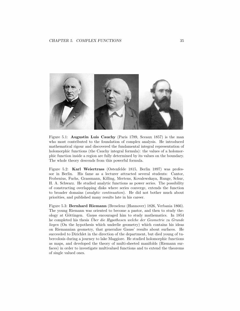
CHAPTER 5. COMPLEX FUNCTIONS 35
Figure 5.1: Augustin Luis Cauchy (Paris 1789, Sceaux 1857) is the manwho most contributed to the foundation of complex analysis. He introducedmathematical rigour and discovered the fundamental integral representation ofholomorphic functions (the Cauchy integral formula): the values of a holomor-phic function inside a region are fully determined by its values on the boundary.The whole theory descends from this powerful formula.
Figure 5.2: Karl Weiertrass (Ostenfelde 1815, Berlin 1897) was profes-sor in Berlin. His fame as a lecturer attracted several students: Cantor,Frobenius, Fuchs, Grassmann, Killing, Mertens, Kovalewskaya, Runge, Schur,H. A. Schwarz. He studied analytic functions as power series. The possibilityof constructing overlapping disks where series converge, extends the functionto broader domains (analytic continuation). He did not bother much aboutpriorities, and published many results late in his career.
Figure 5.3: Bernhard Riemann (Breselenz (Hannover) 1826, Verbania 1866).The young Riemann was oriented to become a pastor, and then to study the-ology at Gottingen. Gauss encouraged him to study mathematics. In 1854he completed his thesis Uber die Hypothesen welche der Geometrie zu Grundeliegen (On the hypothesis which underlie geometry) which contains his ideason Riemannian geometry, that generalize Gauss’ results about surfaces. Hesucceeded to Dirichlet in the direction of the department, but died young of tu-bercolosis during a journey to lake Maggiore. He studied holomorphic functionsas maps, and developed the theory of multi-sheeted manifolds (Riemann sur-faces) in order to investigate multivalued functions and to extend the theoremsof single valued ones.
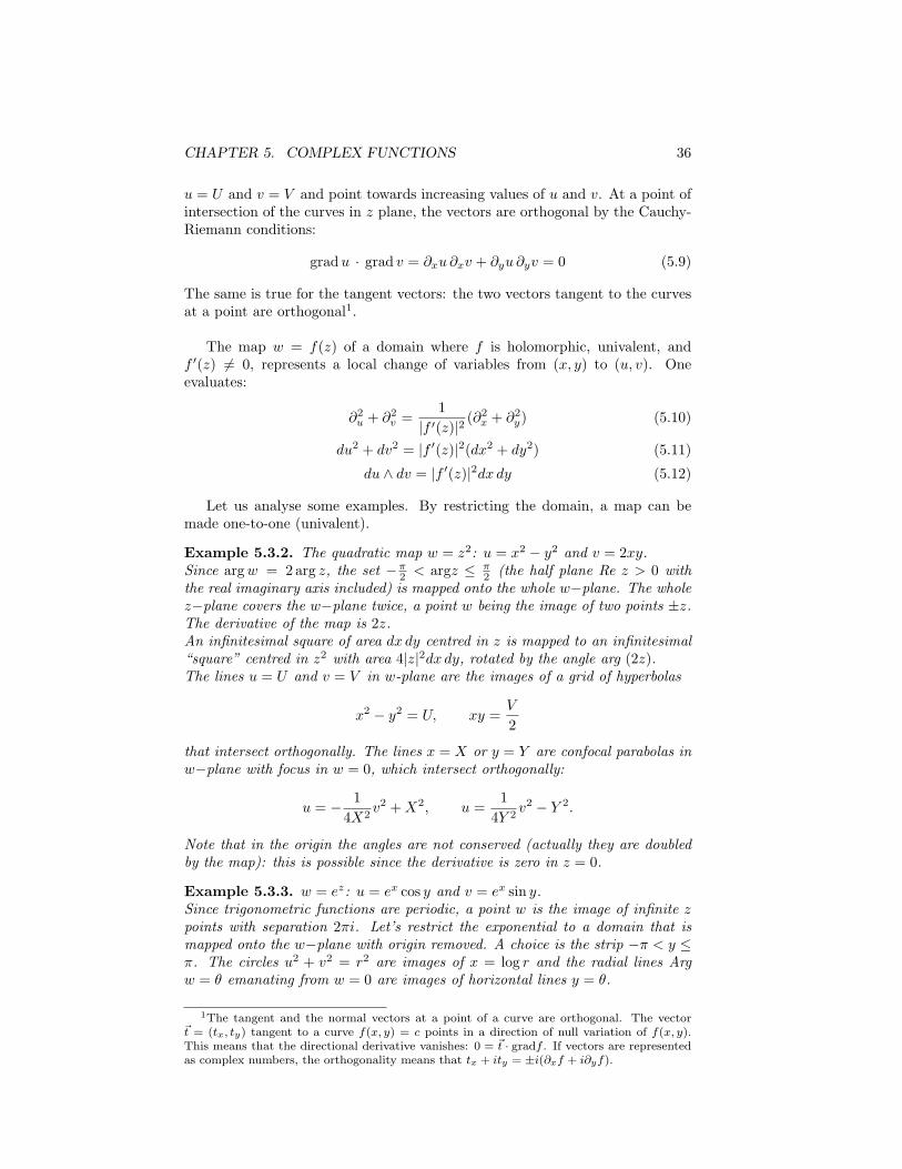
CHAPTER 5. COMPLEX FUNCTIONS 36
u = U and v = V and point towards increasing values of u and v. At a point ofintersection of the curves in z plane, the vectors are orthogonal by the Cauchy-Riemann conditions:
gradu · grad v = ∂xu ∂xv + ∂yu ∂yv = 0 (5.9)
The same is true for the tangent vectors: the two vectors tangent to the curvesat a point are orthogonal1.
The map w = f(z) of a domain where f is holomorphic, univalent, andf ′(z) = 0, represents a local change of variables from (x, y) to (u, v). Oneevaluates:
∂2u + ∂2v =1
|f ′(z)|2(∂2x + ∂2y) (5.10)
du2 + dv2 = |f ′(z)|2(dx2 + dy2) (5.11)
du ∧ dv = |f ′(z)|2dx dy (5.12)
Let us analyse some examples. By restricting the domain, a map can bemade one-to-one (univalent).
Example 5.3.2. The quadratic map w = z2: u = x2 − y2 and v = 2xy.Since argw = 2arg z, the set −π
2 < argz ≤ π2 (the half plane Re z > 0 with
the real imaginary axis included) is mapped onto the whole w−plane. The wholez−plane covers the w−plane twice, a point w being the image of two points ±z.The derivative of the map is 2z.An infinitesimal square of area dx dy centred in z is mapped to an infinitesimal“square” centred in z2 with area 4|z|2dx dy, rotated by the angle arg (2z).The lines u = U and v = V in w-plane are the images of a grid of hyperbolas
x2 − y2 = U, xy =V
2
that intersect orthogonally. The lines x = X or y = Y are confocal parabolas inw−plane with focus in w = 0, which intersect orthogonally:
u = − 1
4X2v2 +X2, u =
1
4Y 2v2 − Y 2.
Note that in the origin the angles are not conserved (actually they are doubledby the map): this is possible since the derivative is zero in z = 0.
Example 5.3.3. w = ez: u = ex cos y and v = ex sin y.Since trigonometric functions are periodic, a point w is the image of infinite zpoints with separation 2πi. Let’s restrict the exponential to a domain that ismapped onto the w−plane with origin removed. A choice is the strip −π < y ≤π. The circles u2 + v2 = r2 are images of x = log r and the radial lines Argw = θ emanating from w = 0 are images of horizontal lines y = θ.
1The tangent and the normal vectors at a point of a curve are orthogonal. The vectort = (tx, ty) tangent to a curve f(x, y) = c points in a direction of null variation of f(x, y).This means that the directional derivative vanishes: 0 = t · gradf . If vectors are representedas complex numbers, the orthogonality means that tx + ity = ±i(∂xf + i∂yf).
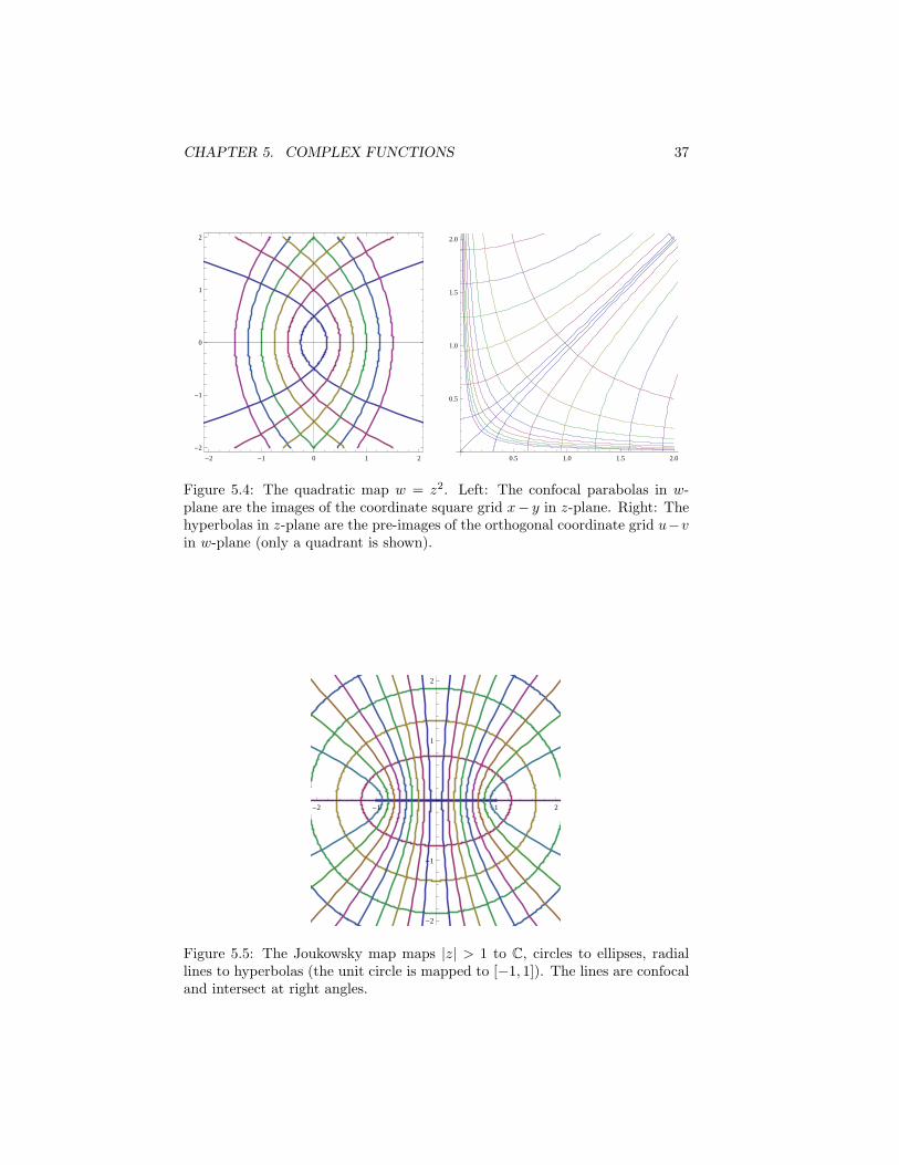
CHAPTER 5. COMPLEX FUNCTIONS 37
-2 -1 0 1 2
-2
-1
0
1
2
0.5 1.0 1.5 2.0
0.5
1.0
1.5
2.0
Figure 5.4: The quadratic map w = z2. Left: The confocal parabolas in w-plane are the images of the coordinate square grid x− y in z-plane. Right: Thehyperbolas in z-plane are the pre-images of the orthogonal coordinate grid u−vin w-plane (only a quadrant is shown).
-2 -1 1 2
-2
-1
1
2
Figure 5.5: The Joukowsky map maps |z| > 1 to C, circles to ellipses, radiallines to hyperbolas (the unit circle is mapped to [−1, 1]). The lines are confocaland intersect at right angles.
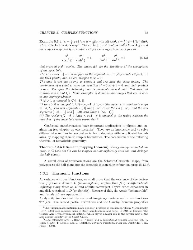
CHAPTER 5. COMPLEX FUNCTIONS 38
Example 5.3.4. w = 12 (z+1/z): u = 1
2 (|z|+1/|z|) cos θ, v = 12 (|z|−1/|z|) sin θ.
This is the Joukowsky’s map2. The circles |z| = eξ and the radial lines Arg z = θare mapped respectively to confocal ellipses and hyperbolas with foci in ±1
u2
cosh2 ξ+
v2
sinh2 ξ= 1,
u2
cos2 θ− v2
sin2 θ= 1 (5.13)
that cross at right angles. The angles ±θ are the directions of the asymptotesof the hyperbola.The unit circle |z| = 1 is mapped to the segment [−1, 1] (degenerate ellipse), ±1are fixed points, and ±i are mapped to w = 0.The map is not one-to-one as points z and 1/z have the same image. Thepre-images of a point w solve the equation z2 − 2wz + 1 = 0 and their productis one. Therefore the Jukowsky map is invertible on a domain that does notcontain both z and 1/z. Some examples of domains and images that are in one-to-one correspondence:i) |z| > 1 is mapped to C/[−1, 1]ii) Im z > 0 is mapped to C/(−∞,−1]∪ [1,∞) (the upper unit semicircle mapsto (-1,1), both real segments (0, 1] and [1,∞] cover the cut [1,∞), and the realsegments (−∞,−1] and [−1, 0) both cover (−∞,−1].)iii) The wedge π/2 − θ < Argz < π/2 + θ is mapped to the region between thebranches of the hyperbola with parameter θ.
Conformal transformations have important applications in physics and en-gineering (see chapter on electrostatics). They are an impressive tool to solvedifferential equations in two real variables in domains with complicated bound-aries, by mapping them to simpler boundaries. The cornerstone is the followingtheorem, of remarkable generality:
Theorem 5.3.5 (Riemann mapping theorem). Every simply connected do-main in C (but not C) can be mapped bi-olomorphically onto the unit disk (orthe half plane).
A useful class of transformations are the Schwarz-Christoffel maps, frompolygons to the half-plane (for the rectangle it is an elliptic function, prop.15.4.1)3.
5.3.1 Harmonic functions
At variance with real functions, we shall prove that the existence of the deriva-tive f ′(z) on a domain D (holomorphism) implies that f(z) is differentiableinfinitely many times on D and admits convergent Taylor series expansion inany disk contained in D (analyticity). Because of this, the words “holomorphic”and “analytic” are equivalent.Analyticity implies that the real and imaginary parts u and v are functionsC∞(D). The second partial derivatives and the Cauchy-Riemann properties
2The Russian mathematician, plane designer, professor of mechanics Nikolay Y. Joukowsky(1847, 1921) used complex maps to study aerodynamics and flows. In 1918 he founded TheCentral Aero-Hydrodynamical Institute, which played a major role in the development of theaero-cosmic industry of the Soviet Union.
3Good references are: P. Henrici, Applied and computational complex analysis, vol. 3,Wiley (1976); T. Driscoll and L. Trefethen, Schwarz-Christoffel mapping, Cambridge Univ.Press. (2002).
CHAPTER 5. COMPLEX FUNCTIONS 39
show that the real and imaginary parts of a holomorphic function areharmonic functions on the (open) domain:
∇2u = 0, ∇2v = 0 (∇2 = ∂2x + ∂2y) (5.14)
Given a harmonic function u(x, y) on a domain D, the Cauchy-Riemann equa-tions may be solved for v(x, y), and a holomorphic function f = u+iv is obtainedon D (up to a constant).
Proposition 5.3.6. If φ(u, v) is harmonic on Dw (a domain in the plane w =u + iv) and if f : Df → Dw is a holomorphic map, then φ(u(x, y), v(x, y)) isharmonic on Df .
Proof. Direct evaluation of partial derivatives checks the statement. In alter-native, φ is the real part of a holomorphic function g(w). Then g(f(z)) isholomorphic in the variable z, and Re g(f(z)) is harmonic.
Example 5.3.7. The function ex2−y2
cos(xy) is harmonic because it is the real
part of the holomorphic function ez2
.The function 1/z is holomorphic on C/0, then its real part x/(x2 + y2) isharmonic on C/0.
5.4 Inverse functions
Let f be a holomorphic function on a domain D; we discuss conditions for theexistence of a holomorphic inverse function f−1.
Definition 5.4.1. A function g is a branch of f−1 with domain U ⊆ f(D) if:1) g is continuous on U ,2) f(g(w)) = w for all w ∈ U .
Remark 5.4.2. The branch function g is univalent (injective) on U if:
g(w1) = g(w2) ⇒ f(g(w1)) = f(g(w2)) and w1 = w2
As a special case of the implicit function theorem in two real variables, we statethe important result
Theorem 5.4.3 (Inverse function theorem). Suppose that f(z) is holomorphicon a domain D, and g(w) is a branch of f−1(w) with domain U . Let f(z0) =w0 ∈ U ; if f ′(z0) = 0 then g is differentiable at w0 and g′(w0) = 1/f ′(z0).Consequently, if f ′(z) = 0 in g(U), then g is holomorphic on U and
g′(w) =1
f ′(g(w))(5.15)
We now discuss the analytic structure of some relevant inverse functions. Inthese examples, the branch is chosen in order to reproduce the inverse functionof real analysis, when restricted to real variable (principal branch).
CHAPTER 5. COMPLEX FUNCTIONS 40
5.4.1 The square root
The function f(z) = z2 maps C to a double cover of the w−plane. It is useful toview the image as a two-sheet Riemann surface, i.e. two copies of the w−plane.In real analysis, the square root u =
√x is defined on the half-line x ≥ 0, and
maps the half-line monotonically to u ≥ 0. Therefore, a convenient choice is toidentify the first sheet as the image of the half-plane
−π2< Arg z <
π
2
which includes the positive real axis. The first sheet has a cut: the negativereal axis Arg w = π, which is the image of the imaginary axis in z plane. Thesecond sheet is the image of the half-plane π > |Argz| > π
2 . The two sheetsshare an edge: the line Arg w = π.
By walking anticlockwise on a circle around the origin z = 0 starting at Argz = −π/2, the image point walks in the first sheet starting at Arg w = π. AtArg z = π/2 a full circle is run in the first sheet, and the walker enters thesecond sheet being at the other edge of the cut Arg w = π. Another circle iscompleted as Arg z = 3π/2. At this point we are again at Arg z = −π/2, i.e.the image point is on the side of the cut where the walk in the first sheet started.
The principal branch of the square root has domain in the first sheet,
√: ρeiθ → √
ρeiθ/2, |θ| < π (5.16)
The half line (−∞, 0] = w s.t. Argw = π is a branch cut, where the squareroot is discontinuous. Near the cut:√
−|x|+ iϵ = i√|x|,
√−|x| − iϵ = −i
√|x|
On the domain C/(−∞, 0] the principal branch is holomorphic and
d
dw
√w =
1
2√w
(5.17)
5.4.2 The logarithm
The function f(z) = ez is defined for all z but, being periodic, it is not invert-ible. On a strip y0 − π < Im z < y0 + π the map is one-to-one with the w-planewith a cut given by the half-line arg w = y0 + π removed. The whole z-plane ismapped to a helix (the Riemann surface of the log). It is a stack of an infinitenumber of sheets (copies of w-plane with cut); each sheet is a domain of a branchof the log: logw = log |w| + i argw (y0 + (2k − 1)π < argw < y0 + (2k + 1)π);it has discontinuity 2πi across the cut if one remains on the same sheet. TheRiemann surface allows one to enter new sheets by crossing the cut: a 2π ascentround the helix axis moves from one sheet to another, where the new branch oflogw differs by 2πi from the previous one.A walk parallel to the imaginary axis in z-plane in the positive direction corre-sponds to a helicoidal path in the Riemann surface.A value y0 (modulo 2π) fixes the cuts; each sheet defines a branch of the logwhich is analytic with derivative
d
dwlogw =
1
elogw=
1
w(5.18)
CHAPTER 5. COMPLEX FUNCTIONS 41
The principal log (Log) is the branch on the first sheet with the choice y0 = 0.Its domain is C/(−∞, 0], where Log z = log |z|+ iArgz, (|Argz| < π).
Chapter 6
ELECTROSTATICS
Several two-dimensional problems (or three-dimensional ones, with a directionof translation invariance) in electrostatics, magnetostatics, fluid-dynamics, elas-ticity, may be elegantly solved in the complex plane, with proper conformalmaps that take care of the geometry. In this chapter we consider electrostatics1
(c.g.s. units are used).
6.1 The fundamental solution
The fundamental solution or Green function2 of 2D electrostatics is the solutionof Poisson’s equation for a unit point charge localized at z′ = x′ + iy′:
∂2φ
∂x2+∂2φ
∂y2= −4π δ(x− x′)δ(y − y′) (6.1)
The solution is easily obtained if the point charge is viewed as the section ofa wire orthogonal to the plane, with unit linear charge. The 3D electrostaticfield E is radial and Gauss’ theorem applied to a cylinder coaxial with the wiregives |E(x, y)| = 2/
√(x− x′)2 + (y − y′)2. The electrostatic potential in 2D of
a point unit charge is E(x, y) = −∇φ i.e.:
φ (x, y) = − log[(x− x′)2 + (y − y′)2
](6.2)
By the superposition principle (linearity of Poisson’s equation), the electrostaticpotential generated by a general charge distribution is:
φ (x, y) = −∫dx′ dy′ log [(x− x′)2 + (y − y′)2] ρ(x′, y′)
1A specialized text in this topic is: E. Durand, Electrostatique, 3 voll, Masson, Paris 1964.2George Green (Nottingham 1793, 1841) was a miller. For more than forty years he worked
hard in his father’s windmill, while self-teaching mathematics and physics. In 1828 he pub-lished at his own expense his most important and astonishing paper: Essay on the applicationof mathematical analysis to the theories of electricity and magnetism, that contains the firstexposition of the theory of potential. After his father’s death, he applied to Cambridge’s uni-versity, and graduated in mathematics in 1838 (the same year as Sylvester). After his deathhis achievements were rescued from obscurity by Lord Kelvin, and are nowadays an importanttool in every area of physics, including quantum field theory (see J. Schwinger, The Greeningof quantum Field Theory: George and I. arXiv:hep-ph/9310283).
42
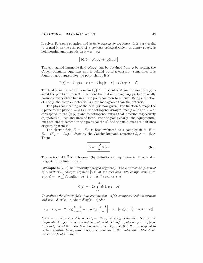
CHAPTER 6. ELECTROSTATICS 43
It solves Poisson’s equation and is harmonic in empty space. It is very usefulto regard it as the real part of a complex potential which, in empty space, isholomorphic and depends on z = x+ iy:
Φ(z) = φ(x, y) + iψ(x, y)
The conjugated harmonic field ψ(x, y) can be obtained from φ by solving theCauchy-Riemann equations and is defined up to a constant; sometimes it isfound by good guess. For the point charge it is
Φ(z) = −2 log(z − z′) = −2 log |z − z′| − i 2 arg (z − z′)
The fields φ and ψ are harmonic in C/z′. The cut of Φ can be chosen freely, toavoid the points of interest. Therefore the real and imaginary parts are locallyharmonic everywhere but in z′, the point common to all cuts. Being a functionof z only, the complex potential is more manageable than the potential.
The physical meaning of the field ψ is now given. The function Φ maps thez plane to the plane w = φ+ iψ; the orthogonal straight lines φ = U and ψ = Vcorrespond in the (x, y) plane to orthogonal curves that describe respectivelyequipotential lines and lines of force. For the point charge, the equipotentiallines are circles centred in the point source z′, and the field lines are half-linesoriginating from z′.
The electric field E = −∇φ is best evaluated as a complex field: E =Ex − iEy = −∂xφ + i∂yφ; by the Cauchy-Riemann equations ∂yφ = −∂xψ.Then:
E = − d
dzΦ(z) (6.3)
The vector field E is orthogonal (by definition) to equipotential lines, and istangent to the lines of force.
Example 6.1.1 (The uniformly charged segment). The electrostatic potentialof a uniformly charged segment [a, b] of the real axis with charge density σ,
φ(x, y) = −σ∫ b
ads log[(x− s)2 + y2], is the real part of
Φ(z) = −2σ
∫ b
a
ds log(z − s)
To evaluate the electric field (6.3) assume that −d/dz commutes with integrationand use −d log(z − s)/dz = d log(z − s)/ds:
Ex − iEy = −2σ logz − b
z − a= −2σ log
∣∣∣∣ z − b
z − a
∣∣∣∣− 2iσ [arg(z − b)− arg(z − a)]
For z = x ± iϵ, a < x < b, it is Ey = ±2πσ, while Ex is non-zero because theuniformly charged segment is not equipotential. Therefore, at each point of [a, b](and only there) there are two determinations (Ex ± iEy)(x) that correspond tovectors pointing to opposite sides; it is singular at the end-points. Elsewhere,the vector field is unique.
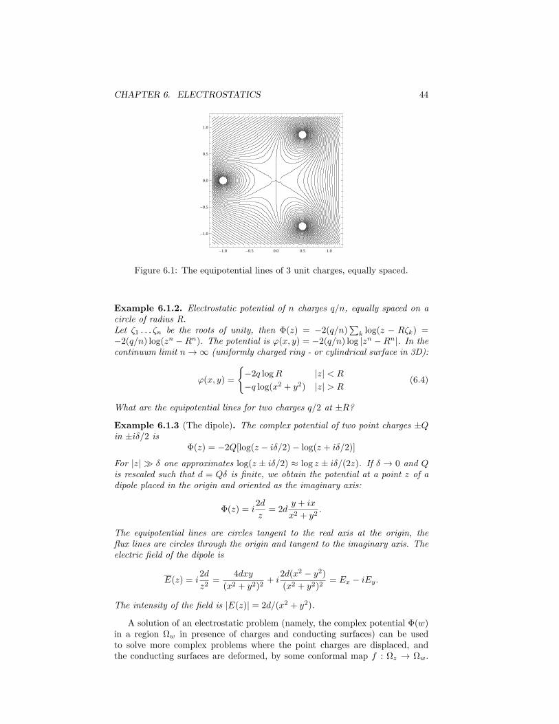
CHAPTER 6. ELECTROSTATICS 44
-1.0 -0.5 0.0 0.5 1.0
-1.0
-0.5
0.0
0.5
1.0
Figure 6.1: The equipotential lines of 3 unit charges, equally spaced.
Example 6.1.2. Electrostatic potential of n charges q/n, equally spaced on acircle of radius R.Let ζ1 . . . ζn be the roots of unity, then Φ(z) = −2(q/n)
∑k log(z − Rζk) =
−2(q/n) log(zn −Rn). The potential is φ(x, y) = −2(q/n) log |zn −Rn|. In thecontinuum limit n→ ∞ (uniformly charged ring - or cylindrical surface in 3D):
φ(x, y) =
−2q logR |z| < R
−q log(x2 + y2) |z| > R(6.4)
What are the equipotential lines for two charges q/2 at ±R?
Example 6.1.3 (The dipole). The complex potential of two point charges ±Qin ±iδ/2 is
Φ(z) = −2Q[log(z − iδ/2)− log(z + iδ/2)]
For |z| ≫ δ one approximates log(z ± iδ/2) ≈ log z ± iδ/(2z). If δ → 0 and Qis rescaled such that d = Qδ is finite, we obtain the potential at a point z of adipole placed in the origin and oriented as the imaginary axis:
Φ(z) = i2d
z= 2d
y + ix
x2 + y2.
The equipotential lines are circles tangent to the real axis at the origin, theflux lines are circles through the origin and tangent to the imaginary axis. Theelectric field of the dipole is
E(z) = i2d
z2=
4dxy
(x2 + y2)2+ i
2d(x2 − y2)
(x2 + y2)2= Ex − iEy.
The intensity of the field is |E(z)| = 2d/(x2 + y2).
A solution of an electrostatic problem (namely, the complex potential Φ(w)in a region Ωw in presence of charges and conducting surfaces) can be usedto solve more complex problems where the point charges are displaced, andthe conducting surfaces are deformed, by some conformal map f : Ωz → Ωw.
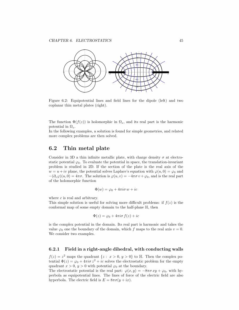
CHAPTER 6. ELECTROSTATICS 45
-4 -2 2 4
-4
-2
2
4
-2 -1 1 2
-1.0
-0.5
0.5
1.0
Figure 6.2: Equipotential lines and field lines for the dipole (left) and twocoplanar thin metal plates (right).
The function Φ(f(z)) is holomorphic in Ωz, and its real part is the harmonicpotential in Ωz.In the following examples, a solution is found for simple geometries, and relatedmore complex problems are then solved.
6.2 Thin metal plate
Consider in 3D a thin infinite metallic plate, with charge density σ at electro-static potential φ0. To evaluate the potential in space, the translation-invariantproblem is studied in 2D. If the section of the plate is the real axis of thew = u+ iv plane, the potential solves Laplace’s equation with φ(u, 0) = φ0 and−(∂vφ)(u, 0) = 4πσ. The solution is φ(u, v) = −4πσ v+φ0, and is the real partof the holomorphic function
Φ(w) = φ0 + 4πiσ w + ic
where c is real and arbitrary.This simple solution is useful for solving more difficult problems: if f(z) is theconformal map of some empty domain to the half-plane H, then
Φ(z) = φ0 + 4πiσ f(z) + ic
is the complex potential in the domain. Its real part is harmonic and takes thevalue φ0 one the boundary of the domain, which f maps to the real axis v = 0.We consider two examples.
6.2.1 Field in a right-angle dihedral, with conducting walls
f(z) = z2 maps the quadrant z : x > 0, y > 0 to H. Then the complex po-tential Φ(z) = φ0 + 4πiσ z2 + ic solves the electrostatic problem for the emptyquadrant x > 0, y > 0 with potential φ0 at the boundary.The electrostatic potential is the real part: φ(x, y) = −8πσ xy + φ0, with hy-perbola as equipotential lines. The lines of force of the electric field are alsohyperbola. The electric field is E = 8πσ(y + ix).
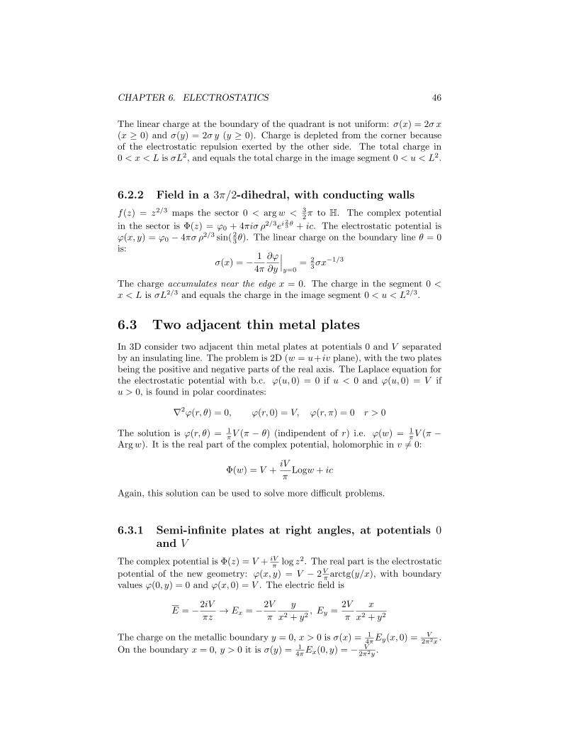
CHAPTER 6. ELECTROSTATICS 46
The linear charge at the boundary of the quadrant is not uniform: σ(x) = 2σ x(x ≥ 0) and σ(y) = 2σ y (y ≥ 0). Charge is depleted from the corner becauseof the electrostatic repulsion exerted by the other side. The total charge in0 < x < L is σL2, and equals the total charge in the image segment 0 < u < L2.
6.2.2 Field in a 3π/2-dihedral, with conducting walls
f(z) = z2/3 maps the sector 0 < argw < 32π to H. The complex potential
in the sector is Φ(z) = φ0 + 4πiσ ρ2/3ei23 θ + ic. The electrostatic potential is
φ(x, y) = φ0 − 4πσ ρ2/3 sin( 23θ). The linear charge on the boundary line θ = 0is:
σ(x) = − 1
4π
∂φ
∂y
∣∣∣y=0
= 23σx
−1/3
The charge accumulates near the edge x = 0. The charge in the segment 0 <x < L is σL2/3 and equals the charge in the image segment 0 < u < L2/3.
6.3 Two adjacent thin metal plates
In 3D consider two adjacent thin metal plates at potentials 0 and V separatedby an insulating line. The problem is 2D (w = u+ iv plane), with the two platesbeing the positive and negative parts of the real axis. The Laplace equation forthe electrostatic potential with b.c. φ(u, 0) = 0 if u < 0 and φ(u, 0) = V ifu > 0, is found in polar coordinates:
∇2φ(r, θ) = 0, φ(r, 0) = V, φ(r, π) = 0 r > 0
The solution is φ(r, θ) = 1πV (π − θ) (indipendent of r) i.e. φ(w) = 1
πV (π −Argw). It is the real part of the complex potential, holomorphic in v = 0:
Φ(w) = V +iV
πLogw + ic
Again, this solution can be used to solve more difficult problems.
6.3.1 Semi-infinite plates at right angles, at potentials 0and V
The complex potential is Φ(z) = V + iVπ log z2. The real part is the electrostatic
potential of the new geometry: φ(x, y) = V − 2Vπ arctg(y/x), with boundary
values φ(0, y) = 0 and φ(x, 0) = V . The electric field is
E = −2iV
πz→ Ex = −2V
π
y
x2 + y2, Ey =
2V
π
x
x2 + y2
The charge on the metallic boundary y = 0, x > 0 is σ(x) = 14πEy(x, 0) =
V2π2x .
On the boundary x = 0, y > 0 it is σ(y) = 14πEx(0, y) = − V
2π2y .
CHAPTER 6. ELECTROSTATICS 47
6.3.2 Two coplanar semi-infinite metallic plates, with gap
The thin plates have potentials 0 and V and are separated by a gap of width2. In the plane z = x + iy, the plates are the semi-infinite lines x ≤ −1 andx ≥ 1 of the real axis. The electrostatic potential solves Laplace’s equation withboundary conditions φ(x, 0) = 0 if x ≤ −1 and φ(x, 0) = V if x ≥ 1. The b.c.are implemented by a conformal map.The domain where φ is harmonic (z-plane with two cuts in the real axis) is theimage of the half-plane H = w : Imw > 0 for the Jukowski’s map
z =1
2
(w +
1
w
)In components Jukowski’s map is (w = reiθ, 0 ≤ θ ≤ π):
x =1
2
(r +
1
r
)cos θ, y =
1
2
(r − 1
r
)sin θ
The half-line θ = 0 is mapped to the cut x ≥ 1, y = 0, while the half-line θ = π ismapped to the other cut x ≤ −1, y = 0. The complex potential of the problemwith the gap is Φ(z) = V + iV
π Logw(z), so that φ(x, y) = 1πV [π−θ(x, y)]. With
some algebra: cos θ = ± 12 [√(x+ 1)2 + y2 −
√(x− 1)2 + y2].
The equipotential lines are lines of constant θ(x, y), i.e. the images in z planeof radii in w plane: they are hyperbola with foci ±1. The lines of force are theimages of circles (constant r), i.e. ellipses with foci ±1 (orthogonal to hyperbolaand to the two cuts).
6.4 Point charge and semi-infinite conductor
Consider of a grounded semi-infinite conductor and a parallel wire at distancey′, with linear charge density Q. The charged wire induces a surface charge thatcontributes to the electrostatic potential. In 2D the problem is that of a pointcharge Q in z′ = x′ + iy′ (y′ > 0) in presence of the half plane Im z ≤ 0 atpotential zero. For y → 0, the lines of force are perpendicular to the real axis.
The evaluation of the field is done by replacing the semi-infinite conductorwith an image charge −Q in z′. By symmetry, the real axis has constant (zero)potential. The complex field is:
Φ(z) = −2Q log(z − z′) + 2Q log(z − z′) + c (6.5)
The real part is the electrostatic potential of the pair ±Q, which is equivalentto the system “real charge and grounded conductor”:
φ(x, y) = −Q log(x− x′)2 + (y − y′)2
(x− x′)2 + (y + y′)2+Re c
It is constant for y = 0, and equal to zero for Re c = 0. The complex electricfield at the surface is
(Ex − iEy)(x+ i0) =2Q
x− z′− 2Q
x− z′= i
4Qy′
(x− x′)2 + y′2
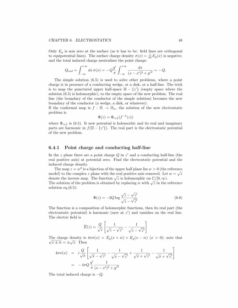
CHAPTER 6. ELECTROSTATICS 48
Only Ey is non zero at the surface (as it has to be: field lines are orthogonalto equipotential lines). The surface charge density σ(x) = 1
4πEy(x) is negative,and the total induced charge neutralizes the point charge:
Qind =
∫ +∞
−∞dxσ(x) = −Q
y′
π
∫ +∞
−∞
dx
(x− x′)2 + y′2= −Q.
The simple solution (6.5) is used to solve other problems, where a pointcharge is in presence of a conducting wedge, or a disk, or a half-line. The trickis to map the punctured upper half-space H − z′ (empty space where thesolution (6.5) is holomorphic), to the empty space of the new problem. The realline (the boundary of the conductor of the simple solution) becomes the newboundary of the conductor (a wedge, a disk, or whatever).If the conformal map is f : H → Ωw, the solution of the new electrostaticproblem is
Φ(z) = Φref (f−1(z))
where Φref is (6.5). It new potential is holomorhic and its real and imaginaryparts are harmonic in f(H − z′). The real part is the electrostatic potentialof the new problem.
6.4.1 Point charge and conducting half-line
In the z plane there are a point charge Q in z′ and a conducting half-line (thereal positive axis) at potential zero. Find the electrostatic potential and theinduced charge density.
The map z = w2 is a bijection of the upper half plane Im w > 0 (the referencemodel) to the complex z plane with the real positive axis removed. Let w =
√z
denote the inverse map. The function√z is holomorphic on C/[0,∞).
The solution of the problem is obtained by replacing w with√z in the reference
solution eq.(6.5):
Φ(z) = −2Q log
√z −
√z′
√z −
√z′
(6.6)
The function is a composition of holomorphic functions, then its real part (theelectrostatic potential) is harmonic (save at z′) and vanishes on the real line.The electric field is
E(z) =Q√z
[1
√z −
√z′
− 1√z −
√z′
]The charge density is 4πσ(x) = Ey(x + iϵ) + Ey(x − iϵ) (x > 0); note that√x± iϵ = ±
√x. Then
4πσ(x) = iQ√x
[1
√x−
√z′
− 1√x−
√z′
+1
√x+
√z′
− 1√x+
√z′
]
= − 4πQy′
π
1
(x− x′)2 + y′2
The total induced charge is −Q.
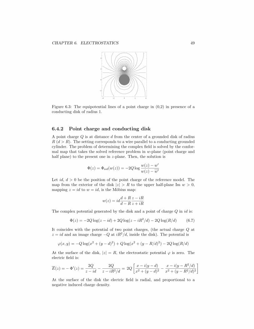
CHAPTER 6. ELECTROSTATICS 49
-4 -2 0 2 4
-2
0
2
4
Figure 6.3: The equipotential lines of a point charge in (0,2) in presence of aconducting disk of radius 1.
6.4.2 Point charge and conducting disk
A point charge Q is at distance d from the center of a grounded disk of radiusR (d > R). The setting corresponds to a wire parallel to a conducting groundedcylinder. The problem of determining the complex field is solved by the confor-mal map that takes the solved reference problem in w-plane (point charge andhalf plane) to the present one in z-plane. Then, the solution is
Φ(z) = Φref(w(z)) = −2Q logw(z)− w′
w(z)− w′
Let id, d > 0 be the position of the point charge of the reference model. Themap from the exterior of the disk |z| > R to the upper half-plane Im w > 0,mapping z = id to w = id, is the Mobius map:
w(z) = idd+R
d−R
z − iR
z + iR
The complex potential generated by the disk and a point of charge Q in id is:
Φ(z) = −2Q log(z − id) + 2Q log(z − iR2/d)− 2Q log(R/d) (6.7)
It coincides with the potential of two point charges, (the actual charge Q atz = id and an image charge −Q at iR2/d, inside the disk). The potential is
φ(x, y) = −Q log(x2 + (y − d)2) +Q log(x2 + (y −R/d)2)− 2Q log(R/d)
At the surface of the disk, |z| = R, the electrostatic potential φ is zero. Theelectric field is:
E(z) =− Φ′(z) =2Q
z − id− 2Q
z − iR2/d= 2Q
[x− i(y − d)
x2 + (y − d)2− x− i(y −R2/d)
x2 + (y −R2/d)2
]At the surface of the disk the electric field is radial, and proportional to anegative induced charge density.
CHAPTER 6. ELECTROSTATICS 50
-10 -5 0 5 10
-10
-5
0
5
10
Figure 6.4: The semi-infinite planar capacitor.
6.5 The planar capacitor
Consider in 3D an infinite planar capacitor; its section in the complex w = u+ivplane is the infinite strip between two conducting lines v = ±d/2 at potentials±V/2. In the strip the electrostatic potential is linear, φ(u, v) = v (V/d), andit is the real part of the complex potential
Φ(w) = −i Vdw (6.8)
The complex electric field is uniform E = iV/d, i.e. Ey = −V/d. The internalcharge densities are 4πσ = −V/d on the lower plate and 4πσ = V/d on theupper one. This solution (infinite planar capacitor) can be used to study morecomplex geometries.
6.5.1 The semi-infinite planar capacitor
Consider the conformal map
z(w) = 2π(w/d) + e2π(w/d)
It maps conjugate points w,w to conjugate points z, z, then the x axis is asymmetry axis and we study the upper half. In components the map is
x = 2πu
d+ e2π(u/d) cos
(2πv
d
), y = 2π
v
d+ e2π(u/d) sin
(2πv
d
).
The lines (u,±d/2) are mapped to x = 2πd u − e2πu/d, y = ±π. Since x′(u) =
(2π/d)(1 − e2πu/d) = 0 in u = 0, the range of x(u) is (−∞,−1]. Therefore themap takes the lines v = ±d/2 to the half-lines x < −1, y = ±π.The map takes the interior of an infinite capacitor (the strip −d/2 < v < d/2)to the interior and the exterior of a semi-infinite capacitor. If the plates have
CHAPTER 6. ELECTROSTATICS 51
potentials ±V/2, the complex potential of the semi-infinite capacitor is:
Φ(z) = −i Vdw(z)
The solution is interesting for the study of the field near the aperture of a finitecapacitor, and was obtained by Maxwell himself, by this conformal map.
The real axis v = 0 is mapped to x = 2πd u+ e2πu/d, y = 0, i.e. the real axis
of the z plane. The lines parallel to the u−axis, v = (d/2π)c, 0 < c < π, aremapped to lines that run inside the capacitor and, near the end of the capacitor,bend upward. If c > π/2 the lines fold back to the top of the condenser. Theequation of such equipotential lines can be obtained by elimination of u inx = 2π u
d + e2π(u/d) cos c, y = c+ e2π(u/d) sin c:
x = logy − c
sin c+ (y − c) cot c (6.9)
Field lines are orthogonal to them and are the images of segments of constant u,|v| < d/2 inside the infinite capacitor: 2πu/d = c; they are given parametrically(in s ∈ [−π, π]) by eqs. x− c = ec cos s and y − s = ec sin s (see note3).
The electric field is
E(z) = iV
d
(dz
dw
)−1
= iV
2π
1
1 + e2πw(z)/d
Deep in the condenser the field is uniform: Ex ≈ 0 and Ey ≈ −V/2π. It divergesat w = ±id/2, i.e. at the ends of the conducting boundaries of the capacitorz = −1± iπ. To avoid the occurrence of divergent fields near the tips of planarcapacitors, one may deform the shape of the plates to trace equipotential linesv = ±(d/2π)c, i.e. (6.9) (Rogowski’s capacitor).
3Deep in the capacitor (c ≪ −1) it is x = c, −π < y < π. For c ≫ 1 the lines are circulararcs that end on the exterior of the capacitor’s plates, (x− c)2 + y2 = e2c (s finite); for smalls the lines x− c ≈ ec − (1/2)y2e−c are approximately straight segments inside the capacitor,near the aperture.
Chapter 7
COMPLEXINTEGRATION
7.1 Paths and Curves
A path is a continuous map of a real interval to the complex plane,
γ : [a, b] → C, (a < b)
The range of the map is a curve γ, and the path γ(t) is its parameterization.The increasing value of the parameter assigns an orientation to the curve. Sinceintervals are compact sets in R and a path is a continuous function, the curveγ is a compact set1 in C.
We list some definitions that apply to paths, and imply geometric propertiesof the curves (that would be difficult to phrase otherwise):
• A path is closed if γ(a) = γ(b) (we then say that the curve is closed).
• A path is simple if γ(t1) = γ(t2) ⇔ t1 = t2, t1,2 = a, b. The curve doesnot self-intersect, except possibly at the endpoints.A Jordan curve J is a simple closed curve. A theorem of topology (Jordan,Veblen) states that C/J is the union of two disjoint sets: one is boundedand the other is unbounded. They are the interior and the exterior of J .
The complex integral on a curve in C, will be defined for curves that areparametrised by smooth functions γ(t):- γ(t) is differentiable on [a, b],- γ(t) = 0 on [a, b],- γ(t) is continuous on [a, b].The complex number γ(t) = x(t) + iy(t) gives the components of the vectortangent to the curve at γ(t) (we shall often identify a complex number with avector). The tangent vector never vanishes. The vector iγ(t) is normal to thecurve.A path is piecewise smooth if it is continuous (it is a path) and is smooth oneach subinterval of some finite partition of [a, b].
1According to the Heine Borel theorem, a set in C is compact iff it is closed and bounded.
52
CHAPTER 7. COMPLEX INTEGRATION 53
A curve can be given different parameterizations. For example the complexsegment [z1, z2] can be parameterized by γ1(t) = z1 + t(z2 − z1) or by γ2(t) =z1+ t
2(z2−z1), t ∈ [0, 1]; both paths trace the same segment, but with different“time laws”.In general, let γ1 : [a, b] → C be a smooth path, and let τ(s) be a real mapof [a′, b′] to [a, b] with dτ/ds > 0, τ(a′) = a and τ(b′) = b. The smooth pathγ2(s) = γ1(τ(s)) with s ∈ [a′, b′] is a reparameterization of the same curve γ.Given a parameterization γ1(τ) and a reparameterization γ2(s) of a curve, at ageometric point of the curve with coordinates τ or s (τ(s) = τ), the two pathsproduce tangent vectors γ1(τ) and γ2(s) with the same direction (if dτ/ds ispositive):
γ2(s) = γ1(τ)dτ
ds, τ(s) = τ.
If a curve is not simple, the geometric point where the curve self-intersects hastwo or more tangent vectors.
7.2 Complex integration
Given a continuous complex function on a smooth oriented curve, f :γ → C, the integral of f on γ is defined as:∫
γ
f(z) dz =
∫ b
a
dt γ(t)f(γ(t)) (7.1)
where γ(t) is a parameterization of the curve2. The value of the integral doesnot depend on the parameterization of the curve γ: if γ2(s) = γ1(τ(s)) it is∫ b′
a′ds γ2(s)f(γ2(s)) =
∫ b′
a′ds γ1(τ)τ(s)f(γ1(τ(s))) =
∫ b
a
dτ γ1(τ)f(γ1(τ)).
Therefore, the integral of a function on an oriented curve is a geometric object.This is apparent in the equivalent construction of the integral sketched below.Given an oriented curve γ from point a to point b, and a function f continuouson it, consider the sum
n−1∑k=0
(zk+1 − zk) f
(zk+1 + zk
2
)where zk are n+ 1 finitely spaced points of the curve, with z0 = a and zn = b.Omitting technicalities, in the limits n → ∞, |zk+1 − zk| → 0, the sum gives aparameterization-independent definition of an integral. If a parameterization ofthe curve is used: zk+1 − zk = γ(tk+1)− γ(tk) ≈ γ(tk)(tk+1 − tk), and the sumyields the above defined integral.
Remark 7.2.1. If the curve γ is an interval of the real line [a, b], a param-eterisation is γ(x) = x, and the complex integral coincides with the Riemannintegral of a continuous function f : [a, b] → C.
2By expanding the product γ(t) f(γ(t)) = (x+ iy)[u(x, y) + i v(x, y)] one obtains four realRiemann integrals that are well defined, since all functions are continuous on closed intervals.
CHAPTER 7. COMPLEX INTEGRATION 54
Note that the complex integral differs from this one:∫γ
f(z)|dz| =∫ b
a
dt√x2 + y2 u(x(t), y(t)) + i
∫ b
a
dt√x2 + y2 v(x(t), y(t)),
which has the meaning of sum (with imaginary factor) of the “areas” of twofoils with basis on the curve and heights u and v.
Example 7.2.2. Let’s evaluate∫γz2dz on the following curves:
i) the oriented segment from a to b. A parameterization is γ(t) = a+ (b− a)t,with 0 ≤ t ≤ 1. Then γ(t) = (b− a) and∫
[a,b]
z2dz = (b− a)
∫ 1
0
dt [a+ (b− a)t]2 = . . . = 13 (b
3 − a3)
ii) the semicircle σ with diameter [a, b] (from a to b counterclockwise). A pa-rameterization is γ(θ) = 1
2 (a + b) + 12 (a − b)eiθ, 0 ≤ θ ≤ π. It is γ(0) = a,
γ(π) = b, and γ = i2 (a− b)eiθ∫
σ
z2dz = i2 (a− b)
∫ π
0
dθeiθ[12 (a+ b) + 1
2 (a− b)eiθ]2
= 13 (b
3 − a3)
Note that the two integrals give the same result, which only depends on theextrema of the path.
If a curve γ is parameterized by γ(t), t ∈ [a, b], the curve with opposite orienta-tion −γ is parameterized by the path γ(a+ b− t) (on [a, b]). Then:∫
−γ
dzf(z) = −∫ b
a
dt γ(a+ b− t)f(γ(a+ b− t))
=
∫ a
b
ds γ(s)f(γ(s)) = −∫γ
dzf(z)
7.2.1 Two useful inequalities
Proposition 7.2.3. If the complex function f is integrable on a real intervalI = [a, b], then: ∣∣∣∣∣
∫ b
a
dtf(t)
∣∣∣∣∣ ≤∫ b
a
dt|f(t)| (7.2)
Proof. Let∫If = eiθ|
∫If |, then∣∣∣∣∫
I
f(t)dt
∣∣∣∣ = ∫I
e−iθfdt =
∫I
Re(e−iθf) dt ≤∫I
|f |dt.
We used Re∫fdt = Re
∫(u+ iv)dt =
∫u dt =
∫Refdt.
If a complex curve is parameterized as γ(t), the real function |f(γ(t))| iscontinuous on [a, b] and has a maximum. The previous inequality gives:
CHAPTER 7. COMPLEX INTEGRATION 55
Proposition 7.2.4 (Darboux’s inequality). If f is a complex continuousfunction on a smooth path γ, then:∣∣∣∣∫
γ
dzf(z)
∣∣∣∣ ≤ L(γ) supz∈γ
|f(z)| (7.3)
where L(γ) =∫ b
adt|γ(t)| is the length of the path (it is a finite number as γ is
required to have continuous derivative on [a, b]. Then γ1 and γ2 are bounded).
Example 7.2.5. Consider the integral I =∫[0,2+iπ]
dz ez. Darboux’s inequality
gives |I| <√4 + π2 supt∈[0,1] |et(2+iπ)| = e2
√4 + π2. The exact value of the
integral is obtained through the primitive (as explained below): I = e2+iπ −e0 =−e2 − 1, then |I| = e2 + 1.
7.3 Primitive
The evaluation of an integral is straightforward if the function has a primitive.
Definition 7.3.1. If f(z) is continuous on a domain D, a primitive of f is afunction F (z) that is holomorphic on D such that
F ′(z) = f(z), ∀z ∈ D
Proposition 7.3.2. If f is continuous on D and has a primitive on it, and γis a path in D, the integral of f on γ only depends on the endpoints of the path:∫
γ
f(z)dz =
∫ b
a
dt γ(t) f(γ(t)) =
∫ b
a
dt γ(t)F ′(γ(t))
=
∫ b
a
dtd
dtF (γ(t)) = F (γ(b))− F (γ(a)). (7.4)
If the path is closed, γ(b) = γ(a), then the integral is zero.
Example 7.3.3. The function ez is the primitive of ez on C; therefore∫γdζeζ =
ez − ez′on any path from z′ to z.
The existence of a primitive as a holomorphic function is a delicate issue, asit is related to global properties of the domain:
Theorem 7.3.4. Let f(z) be a continuous function on an open connected setD. The following statements are equivalent:1) for any two points a and b in D the integral of f along a (piecewise) smoothpath with endpoints a and b does not depend on the path;2) the integral of f along any closed (piecewise) smooth path in D is zero;3) there is a function F (z) holomorphic at all points of D such that F ′(z) = f(z)at all points of D.
Proof. To prove that 1 → 2, 2 → 1 and 3 → 1 is trivial. The only non-trivialstatement to prove is 1 implies 3. Define F (z) as the integral of f from anarbirtary point a ∈ D to z along a path; by hypothesis 1 the function dependson z (and a) but not on the path.
CHAPTER 7. COMPLEX INTEGRATION 56
To prove holomorphy of F consider a disk with center z contained in D (D isopen), choose z + h in the disk (we’ll take the limit h → 0) and consider thepath from a to z+h obtained by prolonging the path from a to z by the segmentσ = [z, z + h]. Parameterize σ as ζ(t) = z + ht (dζ = hdt). Then:
F (z + h)− F (z)
h=
1
h
∫σ
dζf(ζ) =
∫ 1
0
dtf(z+ht) = f(z)+
∫ 1
0
dt [f(z+ht)−f(z)].
Since f is continuous: ∀ϵ > 0 ∃δ such that |f(z + ht) − f(z)| < ϵ if t|h| < δ,then: ∣∣∣∣F (z + h)− F (z)
h− f(z)
∣∣∣∣ ≤ ∫ 1
0
dt|f(z + ht)− f(z)| ≤ ϵ
if |h| ≤ δ, i.e. F ′(z) = f(z).
7.4 The Cauchy transform
Let γ be a (piecewise) smooth path (open or closed) and f a continuous functionon γ. The following integral,
G1(z) =
∫γ
dζ
2πi
f(ζ)
ζ − z, z /∈ γ, (7.5)
is the Cauchy transform of f . This transform will play an important role inCauchy’s theory of holomorphic function, together with the integrals
Gn(z) =
∫γ
dζ
2πi
f(ζ)
(ζ − z)n, z /∈ γ, n = 2, 3, ... (7.6)
The functions f(ζ)/(ζ − z) are continuous on γ so that the integrals exist.Moreover, being C/γ an open set, there is an open disk centred in z of radiusδz that is not crossed by γ. Then, |ζ − z| > δz for all ζ ∈ γ. Let M be the maxof |f(ζ)| for ζ ∈ γ. By Darboux’s inequality: |Gn(z)| ≤ 1
2πL(γ)M (1/δz)n.
Proposition 7.4.1 (see Ahlfors, page 121). The functions Gn(z), n = 1, 2, . . .are holomorphic in C/γ and G′
n(z) = nGn+1(z).
Proof. Let z ∈ C/γ, and let δz be the radius of a disk centred in z with nointersection with the curve. Let z + h belong to such disk and evaluate:
Gn(z + h)−Gn(z) =
∫γ
dζ
2πif(ζ)
[1
(ζ − z − h)n− 1
(ζ − z)n
]=
∫γ
dζ
2πif(ζ)
(ζ − z)n − (ζ − z − h)n
(ζ − z − h)n(ζ − z)n
= −n∑
k=1
(n
k
)(−1)khk
∫γ
dζ
2πi
f(ζ)
(ζ − z − h)n(ζ − z)k
For all ζ ∈ γ it is: |ζ − z| > δz and |ζ − z − h| > δz − |h|. Then∣∣∣Gn(z + h)−Gn(z)∣∣∣ ≤ LM
2πδnz
n∑k=1
(n
k
)|h|k
(δz − |h|)k
CHAPTER 7. COMPLEX INTEGRATION 57
Since the difference is zero as h→ 0, then Gn(z) is continuous.Next, note that
Gn(z + h)−Gn(z)
h= n
∫γ
dζ
2πi
f(ζ)
(ζ − z − h)n(ζ − z)+O(h),
suggesting that, for h→ 0 the right hand side is nGn+1(z). To prove it, consider
Gn(z + h)−Gn(z)
h− nGn+1(z)
= n
∫γ
dζ
2πi
f(ζ)
ζ − z
[1
(ζ − z − h)n− 1
(ζ − z)n
]+O(h)
In analogy with the proof for continuity, by means of Darboux’s inequality it isshown that G′
n(z) exists and equals nGn+1(z).
Remark 7.4.2 (An instructive remark). Let C be a (anticlockwise) circle withcenter 0 and radius r. The integral of zn along the circle is computed exactlyfor any integer n, and is independent of the radius:∮
C
dz zn = i rn+1
∫ 2π
0
dθ ei(n+1)θ = 2πi δn,−1 (7.7)
The functions 1/z, 1/z2, 1/z3, ... are holomorphic in the punctured plane C0 =C/0. What is special about 1/z to give a non-zero result?The reason is that a primitive in C0 (where the circle runs) exists for all but n =−1. Although 1/z locally has a primitive, the function log z is not holomorphicon C0 because of a branch cut that joins the origin to infinity, and C alwayscrosses crosses the cut.If a ray is cut away from the punctured domain C0 then the log function withbranch cut along the ray is a primitive. The open curve C/a with the singleray-point deleted (call it a) is in D′ and the line integral is the difference ofprimitives at the sides of the cut:∫
C/a
dz
z= log a+ − log a− = 2πi
(2πi is the discontinuity of log z across the cut). Now, it should be clear that,for any simple closed path enclosing the origin it is:∮
γ
dz
z= 2πi
the contribution arising solely from the crossing of the branch cut. The result isobviously invariant under a translation, and introduces the interesting topic ofthe following section.
7.5 Index of a closed path.
Definition 7.5.1. If γ is a (piecewise) smooth closed path and z /∈ γ, the Index(or winding number) of γ with respect to z is
Ind(γ, z) =
∮γ
dζ
2πi
1
ζ − z(7.8)
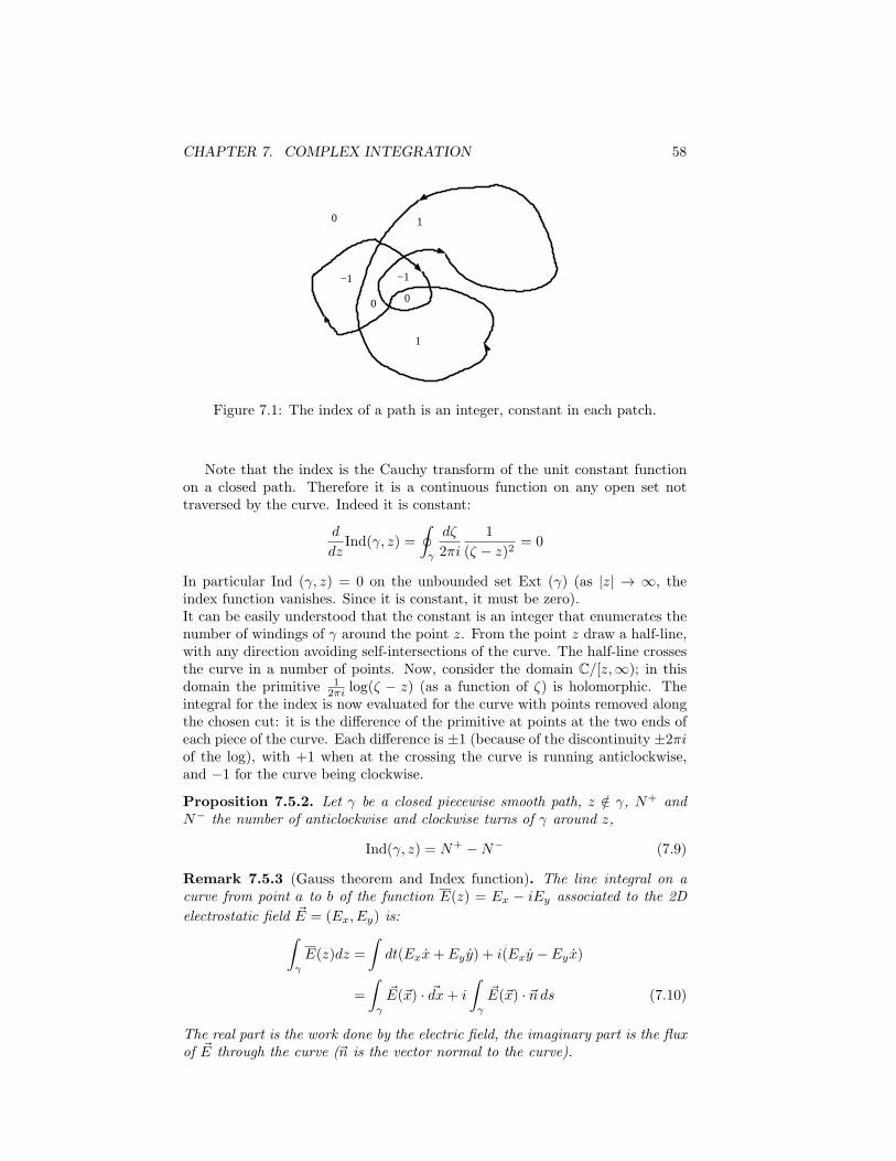
CHAPTER 7. COMPLEX INTEGRATION 58
0 1
−1
0
1
−1
0
Figure 7.1: The index of a path is an integer, constant in each patch.
Note that the index is the Cauchy transform of the unit constant functionon a closed path. Therefore it is a continuous function on any open set nottraversed by the curve. Indeed it is constant:
d
dzInd(γ, z) =
∮γ
dζ
2πi
1
(ζ − z)2= 0
In particular Ind (γ, z) = 0 on the unbounded set Ext (γ) (as |z| → ∞, theindex function vanishes. Since it is constant, it must be zero).It can be easily understood that the constant is an integer that enumerates thenumber of windings of γ around the point z. From the point z draw a half-line,with any direction avoiding self-intersections of the curve. The half-line crossesthe curve in a number of points. Now, consider the domain C/[z,∞); in thisdomain the primitive 1
2πi log(ζ − z) (as a function of ζ) is holomorphic. Theintegral for the index is now evaluated for the curve with points removed alongthe chosen cut: it is the difference of the primitive at points at the two ends ofeach piece of the curve. Each difference is ±1 (because of the discontinuity ±2πiof the log), with +1 when at the crossing the curve is running anticlockwise,and −1 for the curve being clockwise.
Proposition 7.5.2. Let γ be a closed piecewise smooth path, z /∈ γ, N+ andN− the number of anticlockwise and clockwise turns of γ around z,
Ind(γ, z) = N+ −N− (7.9)
Remark 7.5.3 (Gauss theorem and Index function). The line integral on acurve from point a to b of the function E(z) = Ex − iEy associated to the 2D
electrostatic field E = (Ex, Ey) is:∫γ
E(z)dz =
∫dt(Exx+ Ey y) + i(Exy − Eyx)
=
∫γ
E(x) · dx+ i
∫γ
E(x) · n ds (7.10)
The real part is the work done by the electric field, the imaginary part is the fluxof E through the curve (n is the vector normal to the curve).
CHAPTER 7. COMPLEX INTEGRATION 59
Suppose that γ is contained in a domain where the complex potential Φ is holo-morphic. Since E = −dΦ/dz, the line integral is −Φ(b)+Φ(a) and, if the curveis closed, the work and the flux are zero (no net charge is encircled).The complex potential generated by point-charges Qi at zi,
Φ(z) = −2∑i
Qi log(z − zi),
is a holomorphic function except for cuts joining zi to ∞. Such discontinuitiesaffect the imaginary part, therefore the real part of the integral (7.10) on a closedline is zero, i.e. the work done by the field on a closed line is zero. What remainsis ∫
γ
dz E(z) = 2∑j
Qj
∫γ
dz
z − zj= 4πi
∑j
Qj Ind(γ, zj)
This is Gauss’ theorem (the flux is proportional to the total charge encircled).
Chapter 8
CAUCHY’S THEOREMSFOR RECTANGULARDOMAINS
The fundamental theorem for the integral on closed paths of holomorphic func-tions was proven by Cauchy with the requirement that f ′ is continuous. Thecondition was relaxed by Goursat (1900), who proved Cauchy’s theorem for tri-angular paths. A simpler proof was then found for rectangular paths, and isgiven below.The theorem allows for the construction of a primitive. As a consequence, itholds for arbitrary closed paths inside rectangular regions where the functionis holomorphic. The Cauchy integral formula also follows. For entire functionsthe theorems hold everywhere in C.Theorem 8.0.4. If f is holomorphic on a domain, and R is a rectangle in thedomain, with boundary ∂R: ∮
∂R
dzf(z) = 0 (8.1)
Proof. Let L be the length of the diagonal of R, and choose an orientation ofthe boundary. Halve the sides of R and obtain four rectangles R1k (the index 1stands for generation); let I(R1k) be the values of the integrals on the oriented
boundaries of the rectangles. It is I(R) =∑4
k=1 I(R1k) because integrals onshared sides (they have opposite orientations) cancel. Denote I1 the integralwith largest modulus among the four, and R1 the corresponding rectangle. Then|I(R)| ≤
∑k |I(R1k)| ≤ 4|I1|.
A new partition of R1 into four rectangles R2k gives I1 =∑4
k=1 I(R2k). Selectthe rectangle R2k with largest value |I(R2k)|, and let I2 be the value of suchintegral, and R2 the rectangle. It is |I(R)| ≤ 42|I2|.A sequence of rectangles R1 ⊃ R2 ⊃ · · · ⊃ Rn ⊃ · · · may be thus generated,and at generation n:
|I(R)| ≤ 4n|In|The middle points of the rectangles form a Cauchy sequence whose limit pointa belongs to the intersection of all rectangles in the sequence.
60
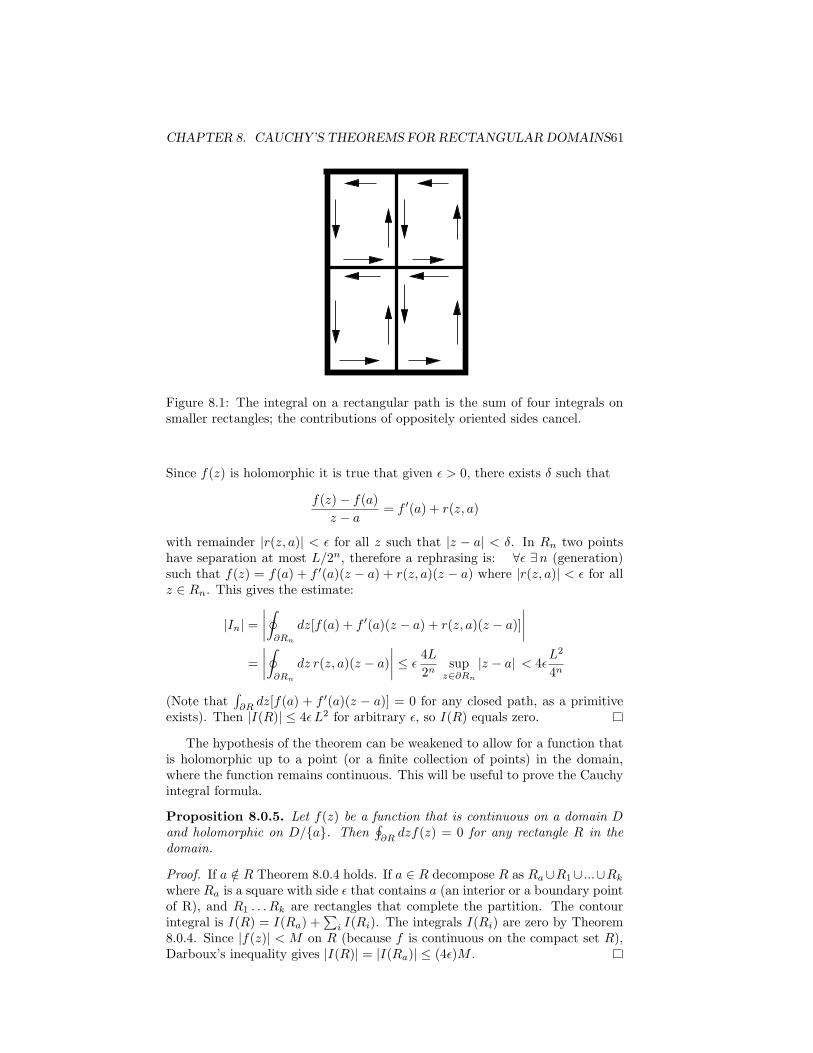
CHAPTER 8. CAUCHY’S THEOREMS FOR RECTANGULARDOMAINS61
Figure 8.1: The integral on a rectangular path is the sum of four integrals onsmaller rectangles; the contributions of oppositely oriented sides cancel.
Since f(z) is holomorphic it is true that given ϵ > 0, there exists δ such that
f(z)− f(a)
z − a= f ′(a) + r(z, a)
with remainder |r(z, a)| < ϵ for all z such that |z − a| < δ. In Rn two pointshave separation at most L/2n, therefore a rephrasing is: ∀ϵ ∃n (generation)such that f(z) = f(a) + f ′(a)(z − a) + r(z, a)(z − a) where |r(z, a)| < ϵ for allz ∈ Rn. This gives the estimate:
|In| =∣∣∣∣∮
∂Rn
dz[f(a) + f ′(a)(z − a) + r(z, a)(z − a)]
∣∣∣∣=
∣∣∣∣∮∂Rn
dz r(z, a)(z − a)
∣∣∣∣ ≤ ϵ4L
2nsup
z∈∂Rn
|z − a| < 4ϵL2
4n
(Note that∫∂Rdz[f(a) + f ′(a)(z − a)] = 0 for any closed path, as a primitive
exists). Then |I(R)| ≤ 4ϵ L2 for arbitrary ϵ, so I(R) equals zero.
The hypothesis of the theorem can be weakened to allow for a function thatis holomorphic up to a point (or a finite collection of points) in the domain,where the function remains continuous. This will be useful to prove the Cauchyintegral formula.
Proposition 8.0.5. Let f(z) be a function that is continuous on a domain Dand holomorphic on D/a. Then
∮∂Rdzf(z) = 0 for any rectangle R in the
domain.
Proof. If a /∈ R Theorem 8.0.4 holds. If a ∈ R decompose R as Ra∪R1∪ ...∪Rk
where Ra is a square with side ϵ that contains a (an interior or a boundary pointof R), and R1 . . . Rk are rectangles that complete the partition. The contourintegral is I(R) = I(Ra) +
∑i I(Ri). The integrals I(Ri) are zero by Theorem
8.0.4. Since |f(z)| < M on R (because f is continuous on the compact set R),Darboux’s inequality gives |I(R)| = |I(Ra)| ≤ (4ϵ)M .
CHAPTER 8. CAUCHY’S THEOREMS FOR RECTANGULARDOMAINS62
Example 8.0.6 (Fourier transform of the Gaussian function).∫ ∞
−∞
dx√2πe−x2−ikx =
1√2e−
14k
2
, k ∈ R (8.2)
Proof: consider the integral∮∂Rdze−z2
on the rectangle with corners −a, b,b + i(k/2) and −a + i(k/2) (0 < a < b). The integral is zero because thefunction is entire. The same integral is the sum of four integrals evaluated onthe sides:
0 =
∫ b
−a
dx e−x2
+ i
∫ k2
0
dy e−(b+iy)2 −∫ b
−a
dx e−(x+ 12 ik)
2
− i
∫ k2
0
dy e−(−a+iy)2
For a, b→ ∞, the integrals in y vanish, and the value of the first integral is√π.
Exercise 8.0.7. Evaluate the moments of the Gaussian distribution:
⟨x2n⟩ =1√π
∫ ∞
−∞dx x2ne−x2
=(2n)!
4nn!(8.3)
(Hint: expand in power series of k both sides of (8.2) and equate coefficients of equal
powers). Prove the useful integral:
1√π
∫ ∞
−∞dx e−x2−xz = e
14 z
2
, z ∈ C. (8.4)
Exercise 8.0.8. By integrating ez2
on the rectangular path with corners 0, s,s+ ih, ih, prove the identity (h→ ∞, separate real and imaginary parts):∫ ∞
0
dx e−x2
sin(2xs) = e−s2∫ s
0
dx ex2
, s ∈ R.
8.1 Cauchy’s theorem in rectangular domains
As a consequence of Cauchy’s theorem for rectangles, within a rectangular do-main R where a function f is holomorphic (or holomorphic up to a finite numberof points where continuity is preserved), a primitive F can be explicitly con-structed. Cauchy’s theorem for arbitrary closed paths and the Cauchy integralformula are then proven.The primitive is built as the integral of f along a path joining a fixed but arbi-trary point in R to z ∈ R. The path is made of two segments at right angles,parallel to the sides of the rectangle. Without loss of generality, we may as-sume that the rectangle has sides parallel to the axes and contains the origin.If z = x+ iy the path is [0, x] ∪ [x, x+ iy] and
F (z) =
∫ x
0
dx′f(x′) + i
∫ y
0
dy′f(x+ iy′)
Proposition 8.1.1. F (z) is holomorphic and F ′(z) = f(z) for all z ∈ R.
CHAPTER 8. CAUCHY’S THEOREMS FOR RECTANGULARDOMAINS63
Proof. Fix z and let h = hx + ihy; because of theorem 8.0.4, it is
F (z + h) =
∫ x+hx
0
dx′f(x′) + i
∫ y+hy
0
dy′f(x+ hx + iy′)
= F (z) +
∫ x+hx
x
dx′f(x′ + iy) + i
∫ y+hy
y
dy′f(x+ hx + iy′)
= F (z) +
∫γ
dζf(ζ)
where the path γ is made of two segments at right angles: [z, z + hx] ∪ [z +hx, z+h]. Divide by h and subtract f(z) from both sides. Note that
∫γdζ = h.
Then:F (z + h)− F (z)
h− f(z) =
1
h
∫γ
dζ [ f(ζ)− f(z) ]
By Darboux’s inequality:∣∣∣∣F (z + h)− F (z)
h− f(z)
∣∣∣∣ ≤ supz∈γ
|f(z)− f(ζ)| |hx|+ |hy||h|
≤ 2 supz∈γ
|f(z)− f(ζ)|
Since f is continuous in z, the limit h → 0 of the r.h.s. is zero. Then F ′ exists(i.e. F is holomorphic) in R and F ′ = f .
With a primitive available at every point, we conclude that the integral of fon any closed (piecewise) smooth path in R is zero1:
Theorem 8.1.2 (Cauchy’s theorem in rectangular domains).∮γ
dzf(z) = 0 (8.5)
Exercise 8.1.3 (Fresnel integrals). Obtain the integrals:∫ ∞
0
dx cos(x2) =
∫ ∞
0
dx sin(x2) =
√2π
4
Hint: consider the null integral∮Cdz eiz
2
on the closed path with sides [0, R], [0, Reiπ/4]
and the circular arc Reiθ, 0 ≤ θ ≤ π/4. The integral on the arc is zero for R → ∞(use the inequality sin θ ≥ 2θ/π valid for 0 ≤ θ ≤ π/2 ).
Exercise 8.1.4. Let F (z) be the primitive of an entire function. Show that forany two points in C: ∣∣∣∣F (b)− F (a)
b− a
∣∣∣∣ ≤ supz∈[a,b]
|F ′(z)|
1This property was known to Gauss, who announced it in a letter to Bessel in 1811 [Boyer].Gauss refrained from publishing several results he obtained, if not fully developed. His mottowas pauca sed matura.
CHAPTER 8. CAUCHY’S THEOREMS FOR RECTANGULARDOMAINS64
8.2 Cauchy’s integral formula
Theorem 8.2.1 (Cauchy’s integral formula). If f is a holomorphic functionon a rectangle R, γ is a (piecewise) smooth closed curve in R and a ∈ R/γ, then∮
γ
dζ
2πi
f(ζ)
ζ − a= f(a) Ind(γ, a), a /∈ γ (8.6)
where Ind (γ, a) is the index of the curve at the point a.
Proof. Consider the function
g(ζ) =
f(ζ)− f(a)
ζ − aζ = a,
f ′(a) ζ = a.
g is continuous on C and holomorphic in C/a. Cauchy’s theorem on rectan-gles holds (a may belong to the boundary), and enables the introduction of aprimitive in C/a. Therefore the integral of g on a closed path is zero:
0 =
∮γ
dζ g(ζ) =
∮γ
dζ
2πi
f(ζ)
ζ − a− f(a) Ind(γ, a)
The Cauchy’s integral formula is remarkable: it shows that the values of afunction holomorphic on a bounded region are determined by the values at theboundary of this region!It also shows that the Cauchy transform on a closed path of a holomorphicfunction coincides with the function itself, times the Index function. Sincewe proved in general that the Cauchy transform of a continuous function isholomorphic on C/γ, the following important theorem follows:
Theorem 8.2.2. The derivative f ′ of a function f holomorphic on a rectangleR, is holomorphic on the same rectangle. In the same way, all derivatives f (n)
exist on R and
1
n!Ind(γ, z) f (n)(z) =
∮γ
dz′
2πi
f(z′)
(z′ − z)n+1, z ∈ R/γ (8.7)
The following theorem is the converse of Cauchy’s theorem 10.2, and is hererephrased for rectangles:
Theorem 8.2.3 (Morera2). If the Cauchy integral of a continuous function fvanishes for all (piecewise) smooth paths in R, then f is holomorphic on R.
Proof. The property of vanishing integral on all rectangular paths implies thata primitive exists, i.e. a function F holomorphic on R such that F ′(z) = f(z)for all z ∈ R. Being F holomorphic, also F ′ i.e. f are holomorphic.
2Giacinto Morera (1856, 1907).
CHAPTER 8. CAUCHY’S THEOREMS FOR RECTANGULARDOMAINS65
Proposition 8.2.4 (Mean value theorem). f(z) is the mean value of f onany circle in R centred in z:
f(z) =
∫ 2π
0
dθ
2πf(z + reiθ) (8.8)
Proof. Apply Cauchy’s formula to a circle with center z and radius r.
Example 8.2.5. Let γ be the ellipse |z − 1|+ |z + 1| = 4, consider the integral∮γ
dzeπz
2z − 3i
The point 32 i is in the ellipse, therefore the integral is 2πi
2 eπ(3i/2) = π.
Exercise 8.2.6. Let γ be the circle |z| = 3. Show that∮γ
dzsin z
z2 − 3z + 2= 2πi(sin 2− sin 1)
Chapter 9
ENTIRE FUNCTIONS
Entire functions are holomorphic on the whole complex plane. Polynomials, theexponential and its linear combinations are entire functions. An entire functionadmit primitives (which differ by constants) which are again entire functions.The mean value theorem (8.8) implies the inequality
|f(z)| ≤ supθ∈[0,2π]
|f(z + reiθ)|
for any circle of radius r centred on z. This implies that |f(z)| has no peaks.Indeed, the following remarkable theorem holds:
Theorem 9.0.7 (Liouville’s theorem). If f(z) is an entire function and|f(z)| ≤M for all z ∈ C, then f(z) is constant.
Proof. Given a point z and a circle C with center 0 and radius R > |z|, theCauchy integral formula gives:
f(z)− f(0) =
∮C
dζ
2πif(ζ)
[1
ζ − z− 1
ζ
]=
∮C
dζ
2πi
zf(ζ)
(ζ − z)ζ= z
∫ 2π
0
dθ
2π
f(Reiθ)
Reiθ − z
In the inequality
|f(z)− f(0)| ≤ |z|∫ 2π
0
dθ
2π
∣∣∣∣ f(Reiθ)Reiθ − z
∣∣∣∣ ≤ |z|M maxθ
1
|Reiθ − z|= M
|z|R− |z|
.
R can be arbitrarily large, then f(z)−f(0) = 0 for all z, i.e. f(z) is constant.
In the proof, the boundedness of f is needed only on the path C. This leadsto several generalizations, like this one:
Corollary 9.0.8. If f(z) is entire and limz→∞ |f(z)| = 0, then f(z) = 0.
Proof. By hypothesis: ∀ϵ > 0 ∃Rϵ such that |f(z)| < ϵ if |z| > Rϵ. Then,repeating the proof of Liouville’s theorem we end with |f(z)−f(0)| < ϵ|z|/(R−|z|) for all R > Rϵ. We conclude that f(z) is constant, and the constant mustbe zero.
Suppose that f is entire and f(z) ∼ az+b for |z| → ∞. Then f(z)−(az+b) →0 at infinity i.e. f(z) = az + b everywhere. More generally, if f(z) ∼ zn atinfinity, then f(z) is a polynomial of degree n.
66
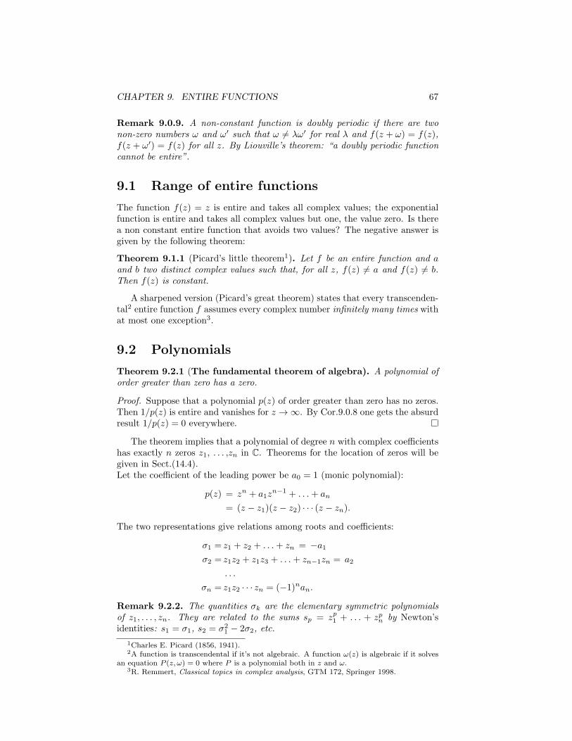
CHAPTER 9. ENTIRE FUNCTIONS 67
Remark 9.0.9. A non-constant function is doubly periodic if there are twonon-zero numbers ω and ω′ such that ω = λω′ for real λ and f(z + ω) = f(z),f(z + ω′) = f(z) for all z. By Liouville’s theorem: “a doubly periodic functioncannot be entire”.
9.1 Range of entire functions
The function f(z) = z is entire and takes all complex values; the exponentialfunction is entire and takes all complex values but one, the value zero. Is therea non constant entire function that avoids two values? The negative answer isgiven by the following theorem:
Theorem 9.1.1 (Picard’s little theorem1). Let f be an entire function and aand b two distinct complex values such that, for all z, f(z) = a and f(z) = b.Then f(z) is constant.
A sharpened version (Picard’s great theorem) states that every transcenden-tal2 entire function f assumes every complex number infinitely many times withat most one exception3.
9.2 Polynomials
Theorem 9.2.1 (The fundamental theorem of algebra). A polynomial oforder greater than zero has a zero.
Proof. Suppose that a polynomial p(z) of order greater than zero has no zeros.Then 1/p(z) is entire and vanishes for z → ∞. By Cor.9.0.8 one gets the absurdresult 1/p(z) = 0 everywhere.
The theorem implies that a polynomial of degree n with complex coefficientshas exactly n zeros z1, . . . ,zn in C. Theorems for the location of zeros will begiven in Sect.(14.4).Let the coefficient of the leading power be a0 = 1 (monic polynomial):
p(z) = zn + a1zn−1 + . . .+ an
= (z − z1)(z − z2) · · · (z − zn).
The two representations give relations among roots and coefficients:
σ1 = z1 + z2 + . . .+ zn = −a1σ2 = z1z2 + z1z3 + . . .+ zn−1zn = a2
. . .
σn = z1z2 · · · zn = (−1)nan.
Remark 9.2.2. The quantities σk are the elementary symmetric polynomialsof z1, . . . , zn. They are related to the sums sp = zp1 + . . . + zpn by Newton’sidentities: s1 = σ1, s2 = σ2
1 − 2σ2, etc.
1Charles E. Picard (1856, 1941).2A function is transcendental if it’s not algebraic. A function ω(z) is algebraic if it solves
an equation P (z, ω) = 0 where P is a polynomial both in z and ω.3R. Remmert, Classical topics in complex analysis, GTM 172, Springer 1998.
CHAPTER 9. ENTIRE FUNCTIONS 68
Exercise 9.2.3. Prove the following identity for polynomials with simple roots(it is useful for evaluating integrals):
1
p(z)=
n∑k=1
1
p′(zk)
1
z − zk(9.1)
Exercise 9.2.4. If the roots are simple, show that:
p′′(zk)
p′(zk)=∑j =k
2
zk − zj,
∏k
p′(zk) = (−)12n(n−1)
∏i>j
(zi − zj)2. (9.2)
Exercise 9.2.5. Let pk(z) be monic polynomials of degree k = 1, . . . , n − 1.Show that:
det
1 p1(z1) · · · pn−1(z1)1 p1(z2) · · · pn−1(z2)...
......
1 p1(zn) · · · pn−1(zn)
= det
1 z1 · · · zn−1
1
1 z2 · · · zn−12
......
...1 zn · · · zn−1
n
=∏i>j
(zi − zj)
The second matrix is the Vandermonde matrix, which is an important tool inlinear algebra, matrix theory, and polynomial interpolation.
Exercise 9.2.6. By expanding (9.1) in powers of 1/z and equating coefficients,obtain the identities for the roots:
0 =n∑
k=1
zℓkp′(zk)
(ℓ = 0, . . . , n− 2), 1 =n∑
k=1
zn−1k
p′(zk), −a1 =
n∑k=0
znkp′(zk)
, . . .
Exercise 9.2.7. Prove the relations, valid for general polynomials:
p′(z)
p(z)=
n∑k=1
1
z − zk,
p′(z)2 − p′′(z)p(z)
p(z)2=
n∑k=1
1
(z − zk)2
Exercise 9.2.8. If f(z) is an entire funtion and γ is a simple closed pathenclosing the points z = 0, 1, . . . , n show that:∮
γ
dz
2πi
f(z)
z(z − 1) · · · (z − n)=
(−1)n
n!
n∑k=0
(−1)k(n
k
)f(k)
Exercise 9.2.9. Let the simple closed path γ contain the unit disk and let f(z)be an entire function; show that:∮
γ
dz
2πi
f(z)
zn − 1=
1
n
n∑k=1
ωkf(ωk), ω = exp(i 2πn )
CHAPTER 9. ENTIRE FUNCTIONS 69
0.1
0.1
0.2
0.2
0.3
0.30.4
0.4
0.5
0.5
0.6
0.6
0.7
0.7
0.7
0.7
0.8
0.8
0.8
0.8
0.9
0.9
0.9
0.9
11
1.11.1
1.2
1.2
1.3
1.3
1.4
1.4
1.5
1.5
1.6
1.6
1.7
1.7
1.8
1.8
1.9
1.9
2
2
2.1
2.1
2.2
2.2
2.3
2.3
2.4
2.4
2.5
2.5
2.6
2.6
2.7
2.7
-1.0 -0.5 0.0 0.5 1.0
-1.0
-0.5
0.0
0.5
1.0
Figure 9.1: Each label k marks a lemniscate of equation |z2− z√2+1| = k. For
k < 1 the lemniscate is a pair of ovals surrounding the roots.
Miscellanea
Given a monic polynomial of order n with distinct zeros, the set z : |pn(z)| = cis a lemniscate. For c = 0 it consists of n points (the roots), by increasing cit evolves into n distinct ovals encircling the roots. As c is increased the ovalsstart to merge into fewer closed lines. Some general questions have been asked,and describe the growth in modulus of a polynomial. Two nice examples are:1) Cartan’s Lemma: the inequality |pn(z)| > (R/e)n holds outside at most ncircular disks, the sum of the radii being at most 2R.2) The length of the lemniscate |pn(z)| = 1 is not greater than Kn, whereK ≤ 8πe (Borwein, 1995). The result was improved to K ≤ 9.173 (Eremenkoand Hayman, 1999).
Chapter 10
CAUCHY’S THEORYFOR HOLOMORPHICFUNCTIONS
The extension of the theory from rectangular domains to general domains re-quires care. If f is holomorphic on D and has singularities in C/D, the integralof f on a closed path in D may depend on the fact that a singularity is encircledor not by it. This information is carried by the index function: if it is zero thedangerous point is not encircled1.Dixon gave a proof of Cauchy’s theorem and integral formula on general do-mains that solves the topological problem with the index function. The proofis elegant as it only requires Liouville’s theorem for entire functions2.
Theorem 10.0.10 (Dixon). Let γ be a piecewise smooth closed path in a domainD such that Ind (γ, z) = 0 ∀z /∈ D. If f is holomorphic on D:
Ind(γ, z) f(z) =
∮γ
dζ
2πi
f(ζ)
ζ − z(Cauchy’s integral formula) (10.1)
0 =
∮γ
dζ f(ζ) (Cauchy’s theorem) (10.2)
Proof. Consider the function g : D ×D → C
g(ζ, z) =f(ζ)− f(z)
ζ − zfor ζ = z, g(z, z) = f ′(z)
g is continuous in each variable. Next, define the function h : C → C,
h(z) =
∮γ
dζ
2πig(ζ, z) if z ∈ D, h(z) =
∮γ
dζ
2πi
f(ζ)
ζ − zif z ∈ C/D.
1or the path encircles it with an equal number of oppositely oriented loops. In this case itmay be replaced by the union of paths that do not encircle the point.
2John D. Dixon, A brief proof of Cauchy’s integral theorem, Proc. Am. Math. Soc. 29 n.3(1971) 625-26. Peter A. Loeb, A note on Dixon’s proof of Cauchy’s Integral Theorem, Am.Math. Month. 98 n.3 (1991) 242-244. See the books by Lang or Remmert for a presentationof Dixon’s proof.
70
CHAPTER 10. CAUCHY’S THEORY FORHOLOMORPHIC FUNCTIONS71
In particular, if z ∈ D/γ it is
h(z) =
∮γ
dζ
2πi
f(ζ)
ζ − z− f(z)Ind(γ, z)
The key point (not proven here) is that h is entire. Then everything follows: ash(z) → 0 for |z| → ∞, by Liouville’s theorem (Cor. 9.0.8) it is h(z) = 0 on C,and (10.1) is proven.To obtain (10.2), choose a in D/γ and apply (10.1) to the function (z− a)f(z):
Ind(γ, z) (z − a)f(z) =
∮γ
dζ
2πi
ζ − a
ζ − zf(ζ).
Take the limit a→ z.
Corollary 10.0.11. A holomorphic function can be differentiated indefinitelyon its domain.
Exercise 10.0.12. Use Cauchy’s formula to evaluate the useful integral (Hint:z = eiθ): ∫ 2π
0
dθ1
1− 2x cos θ + x2=
2π
1− x2, 0 ≤ x < 1. (10.3)
Chapter 11
POWER SERIES
11.1 Uniform and normal convergence
We consider sequences of functions fn on some abstract set E to C. At eachpoint P ∈ E there is a complex sequence fn(P ), whose convergence is assessedby Cauchy’s criterion.
Point-wise convergence on E. Suppose that ∀P ∈ E the sequence fn(P )converges to a finite complex number. The set of limit values defines a functionf : E → C, and we say that fn → f point-wise on E.Since C is complete, we only need Cauchy’s criterion for convergence:
∀P ∈ E ∀ϵ > 0 ∃Nϵ,P such that |fn(P )− fm(P )| < ϵ ∀m,n > Nϵ,P
Uniform convergence on E. Suppose that the stronger condition occurs:∀P ∈ E the sequence fn(P ) is Cauchy with Nϵ independent of P . Then fnconverges on E, and the distance |fn(P )−fm(P )| is bounded on E by the sameϵ for all P ∈ E, n,m > Nϵ. We say that fn → f uniformly on E:
∀ϵ > 0 ∃Nϵ such that |fn(P )− fm(P )| < ϵ ∀m,n > Nϵ, ∀P ∈ E.
Definition 11.1.1. A series of functions∑
k fk is uniformly convergent on Eif the sequence of partial sums is uniformly convergent on E:
∀ϵ > 0 ∃Nϵ :
∣∣∣∣∣m+n∑
k=m+1
fk(P )
∣∣∣∣∣ < ϵ ∀m > Nϵ, ∀n > 0, ∀P ∈ E. (11.1)
Theorem 11.1.2 (Weierstrass M-criterion). If there are positive constantsMk such that |fk(P )| < Mk for all P ∈ E and
∑kMk < ∞, then the series∑
k fk is uniformly convergent on E.
Proof. Let Sm(P ) be the sequence of partial sums. For all P ∈ E:
|Sm+n(P )− Sm(P )| ≤m+n∑
k=m+1
|fk(P )| ≤m+n∑
k=m+1
Mk < ϵ
for m large enough and all n, because the M−series converges.
72
CHAPTER 11. POWER SERIES 73
Proposition 11.1.3. The geometric series∑
k zk is uniformly convergent on
the closed disk |z| ≤ 1− η, η > 0.
Proof. Use the M−criterion with Mk = (1− η)k.
From now on, E is a set in C. Uniform convergence of a series guaranteesthat integration can be made term by term:
Theorem 11.1.4 (Integral of series). Given a piecewise smooth curve γ in adomain D, a sequence fk of functions continuous on γ, suppose that
∑k fk is
uniformly convergent on γ, then:∫γ
dz
∞∑k=0
fk(z) =
∞∑k=0
∫γ
dz fn(z) (11.2)
Proof. The partial sums Sm(z) are continuous functions on γ which is a compactset, then uniform convergence implies that the limit series S(z) =
∑∞k=0 fn(z)
is continuous on γ, and the integral exists. Uniform convergence on γ meansthat |Sm(z) − S(z)| < ϵ for all m > N and for all z ∈ γ. Darboux’s inequalityshows that summation and integration commute:∣∣∣∣∣
m∑k=0
∫γ
dzfk(z)−∫γ
dz
∞∑k=0
fk(z)
∣∣∣∣∣ ≤∫γ
|dz| |Sm(z)− S(z)| < ϵL(γ)
Uniform convergence on a domain makes the theorem applicable to any curvein the domain. One can also prove that a uniformly convergent series may bederived term by term. However, the requirement of uniform convergence on adomain is very restrictive. Theorem 11.1.4 and derivation term by term, canbe proven under the weaker hypothesis of local uniform convergence (normalconvergence).
Definition 11.1.5. A sequence of functions fn converges normally to f on adomain D if it converges point-wise to f on D and, for any z ∈ D, there is aclosed disk centred in z where convergence is uniform.
Theorem 11.1.6 (Integral of series). Given a piecewise smooth curve γ and asequence of continuous functions fk on D, suppose that the series
∑k fk(z) is
normally convergent on γ. Then∫γ
dz∞∑k=0
fk(z) =∞∑k=0
∫γ
dzfk(z) (11.3)
Theorem 11.1.7. If a sequence fk is normally convergent to f on a domain Dand all functions fk are holomorphic, then f is holomorphic and the sequence
of n-th derivatives f(n)k converges to f (n) normally.
Theorem 11.1.8 (Derivative of series). If the series∑
k fk is normally con-vergent on a domain D, and every term fk is holomorphic on D, then the series
CHAPTER 11. POWER SERIES 74
is holomorphic on D. Moreover, the series can be differentiated term by termany number of times:
dn
dzn
∞∑k=0
fk(z) =
∞∑k=0
dnfkdzn
(z), n = 1, 2, . . . (11.4)
for all z ∈ D, and each differentiated series is normally convergent.
11.2 Power series
A fundamental class of series of complex functions are power series:
f(z) =
∞∑n=0
cn(z − a)n (11.5)
a ∈ C is the center of the power series, the coefficients cn are complex numbers.Two notable examples are the geometric and exponential series. They convergeabsolutely, the first one in the open disk |z| < 1, the second one everywhere.This is a fundamental theorem:
Theorem 11.2.1 (Abel, Weierstrass). If the power series∑
k ck(z − a)k isconvergent at a point z0, then the series converges:1) absolutely for all z in the open disk |z − a| < |z0 − a|,2) uniformly in the closed disk |z − a| ≤ (1− η)|z0 − a|, η > 0.
Proof. 1) We use the comparison criterion. Convergence of the series in z0implies that |ck(z0−a)k| → 0; then, there is a finite N such that |ck(z0−a)k| < 1for all k > N . This means that |ck(z − a)k| is majorized by |(z − a)/(z0 − a)|k.The sum of the latter terms converges (absolutely) for all z in the open disk|z − a| < |z0 − a|.2) If |z−a| ≤ |z0−a|(1−η) it follows that, for k > N , it is |ck(z−a)k| ≤ (1−η)k.Then the convergence is uniform by the Weierstrass’ M-criterion.
The theorem shows that one out of three possibilities occurs:
• z = a is the only point where the series converges.
• There are points z = a where the series converges, but the series divergesat other points.
• The series converges everywhere in C.
The Abel - Weierstrass theorem shows that convergence in z implies convergencein any open disk centred in a of radius r < |z − a|. Case two implies the exis-tence of a radius R such that for |z−a| < R the series converges absolutely (anduniformly in any closed disk strictly contained in it) and diverges in |z−a| > R.The value R is the radius of convergence of the series. If R = ∞ the seriesconverges absolutely everywhere, and uniformly on any closed bounded set.In general nothing can be said about the series on the circle |z − a| = R 1.
1However, if the series converges in a point z0 with |z0−a| = R, a theorem by Abel provesthat on the radius ζ(t) = a+ (z0 − a)t (t ∈ [0, 1]) the series f(t) =
∑ck(z0 − a)ktk converges
uniformly with respect to t and limt→1 f(t) = f(1).
CHAPTER 11. POWER SERIES 75
We give two important formulae for the determination of the radius, whichresult from the sufficient criteria for absolute convergence of series.
Definition 11.2.2. Given an infinite set A ⊂ R bounded above, lim supA (orlimA) is the largest real number a such that ∀ϵ the set a ∈ A : a > a + ϵ isfinite and a ∈ A : a > a− ϵ is infinite.
Theorem 11.2.3 (Cauchy - Hadamard).
1
R= lim supk
k√
|ck| (11.6)
If limk→∞k√|ck| exists, it is equal to 1/R.
Theorem 11.2.4 (Ratio criterion).
lim inf|ck|
|ck+1|≤ R ≤ lim sup
|ck||ck+1|
(11.7)
In particular R = limk→∞|ck|
|ck+1| whenever this limit exists (ck = 0 but for a
finite set of integers).
Example 11.2.5. In∑∞
k=1(2z)2k odd powers are missing and the sequence
n√cn = 2, 0, 2, 0, . . . is not convergent, but its lim sup is 2. Then the series
converges in the disk |z| < 12 (as a geometric series, it converges for |4z2| < 1).
Exercise 11.2.6. Evaluate the radius of convergence of the series:
∞∑k=1
zk
k,
∞∑k=0
z2k
(2k)!,
∞∑k=1
(−1)kz3k,∞∑k=0
zk2
,∞∑k=0
k2zk
Theorem 11.2.7. The power series
S(z) =
∞∑k=0
ck (z − a)k and S′(z) =
∞∑k=1
k ck (z − a)k−1
have the same radius of convergence.
Proof. In the proof we put a = 0. Suppose that S and S′ have radii R and R′
respectively. Since |ckzk| < |z| |kckzk−1| for all z, by the comparison test, theseries S converges absolutely if S′ does, i.e. |z| < R′ is a sufficient condition forS to absolutely converge. Then R ≥ R′.
For z such that |z| < R it is k|z|k−1 < Rk
R−|z| . Then it is |kckzk−1| < 1R−|z| |ckR
k|and the series S′ converges absolutely if S does, i.e. R ≤ R′.We used the inequality 1
1−r > 1 + r + . . . rn−1 > nrn−1, 0 ≤ r < 1.
Corollary 11.2.8. A power series∑
n cn(z−a)n is a holomorphic function onthe open disk of convergence (where it is also infinitely many times differentiable)
Exercise 11.2.9. Evaluate∑∞
n=1 n2zn (Note that z
d
dzzn = nzn).
CHAPTER 11. POWER SERIES 76
Theorem 11.2.10 (Power series for holomorphic functions). Let f beholomorphic in a domain, and let D be an open disk centred in a of radius r inthe domain, with (positively oriented) boundary C. Then, for any z in the disk,f has the power series expansion
f(z) =∞∑k=0
ck(z − a)k, ck =
∮C
dζ
2πi
f(ζ)
(ζ − a)k+1(11.8)
Proof. For any z in the disk D(a, r), f(z) is given by the Cauchy integral
f(z) =
∮C
dζ
2πi
f(ζ)
ζ − z.
Since r = |ζ − a| > |z − a|, the kernel admits an expansion in geometric series
1
ζ − z=
1
ζ − a− (z − a)=
∞∑k=0
(z − a)k
(ζ − a)k+1(11.9)
The sum can be taken out of the integral because the series converges uniformlyin the interior of the disk.
Corollary 11.2.11. A holomorphic function can be differentiated indefinitelyand
f (k)(a) = k!
∮C(a,r)
dζ
2πi
f(ζ)
(ζ − a)k+1(11.10)
Darboux’s inequality gives Cauchy’s Inequality
|f (k)(a)| ≤ k!
rksup
θ∈[0,2π]
|f(a+ reiθ)| (11.11)
Remark 11.2.12. The radius of convergence of the power series centred in aof an analytic function is the largest admissible radius of a disk centred in a inthe domain of analyticity: R = |ξ − a| where ξ is the singular point or branchcut point nearest to a.
Example 11.2.13. The function f(z) = [(z−2i)(z−3)]−1 is singular at z = 2iand z = 3. A power expansion in the origin has radius 2. An expansion withcenter a = 1 has radius 2 because the singular point 3 has distance |3 − 1| = 2smaller than the distance |2i− 1| =
√5 of the singular point 2i.
Exercise 11.2.14. Integrate term by term the geometric series to obtain:
Log(1− z) = −∞∑k=1
zk
k|z| < 1 (11.12)
Exercise 11.2.15. From the expansion (11.12) obtain:
∞∑k=1
ρk
kcos(kθ) = −1
2log(1− 2ρ cos θ + ρ2), ρ < 1.
CHAPTER 11. POWER SERIES 77
Example 11.2.16. The function Log z has the branch cut (−∞, 0]. A powerseries of Log z with center a is initially constructed in a disk D(a, r) that avoidsthe cut, where Log z is holomorphic. If Re a > 0 the radius is r = |a| (the leastdistance of a from the cut), if Re a < 0 this least distance is r = |Im a|. Insidethe disk D(a, r):
Log z =Log a+ Log(za
)= Log a+ Log
(1 +
z − a
a
)with no additional terms ±2πi (to check this requires some simple work). Theexpansion (11.12) gives:
Log z = Log a−∞∑k=1
(−1)k
kak(z − a)k
The right hand side is meaningful in a disk of convergence D(a, |a|) and doesnot distinguish the cases r = Im a or r = |a|. However, if z is taken such that|z| < |a| and the line of sight [a, z] is crossed by the cut, the left hand side differsfrom the right hand side by ±2πi. We are thus evaluating log z on a differentsheet.
Example 11.2.17. Evaluate the coefficients of the power series
etz
1− z=
∞∑n=0
cn(t)zn
It is convenient to compare the series etz = (1−z)∑
n cnzn =
∑n z
n(cn−cn−1),with c0 = 1, c−1 = 0. This gives the recursive rule cn − cn−1 = tn/n! i.e.
cn(t) = 1 + t+t2
2!+ . . .+
tn
n!.
Example 11.2.18. Evaluate the coefficients of the power series
1
z2 + z − 1=
∞∑n=0
cnzn
The radius of convergence of the series is dictated by the size of the smallestroot of the binomial: R = 1
2 (√5 − 1). The quick way to obtain the coefficients
is to write the l.h.s. as a combination of two geometric series. However, thefollowing procedure is interesting.Multiply the series by the denominator to get 1 =
∑n z
n(cn−2 + cn−1 − cn)i.e. cn = cn−1 + cn−2 and c0 = 1 (c−1 = 0). The recursion generates theFibonacci numbers 1, 1, 2, 3, 5, 8, 13, . . . . The general solution can be found: cn =axn1 + bxn2 , where x1,2 solve the quadratic equation x2 − x− 1 = 0 and a, b arespecified by the initial conditions.If x1 is the root with largest modulus, Hadamard’s criterion for the radius of thepower series gives 1/R = |x1|, i.e. R = |x2| (note that x1x2 = 1).The recursion can be written (cn/cn−1) = 1 + (cn−2/cn−1). In the large n limitcn/cn−1 → ϕ and ϕ = 1 + 1/ϕ (then, by the ratio criterion, R = 1/ϕ). Thenumber ϕ = 1
2 (√5+1) is the golden mean, and is the limit of ratios of Fibonacci
numbers. Its continued fraction expansion is peculiar, ϕ = 1+1/(1+/(1+/(1+. . . ), and makes this number the “most irrational” one (Hurwitz developed atheory for rational approximation of irrationals).
CHAPTER 11. POWER SERIES 78
Example 11.2.19. The Euler numbers are the coefficients E2n in the powerseries
1
cos z=
∞∑n=0
(−1)nE2nz2n
(2n)!
The radius of convergence of the series is π/2 (the pole closest to the origin).This gives us the estimate |E2n| ≈ (2n)!(2/π)2n (up to factors that grow lessthan powers of n)2. Multiplication by cos z gives a Cauchy product of series:
1 =∞∑k=0
z2k(−1)k
(2k)!
k∑ℓ=0
(2k
2ℓ
)E2ℓ
Comparison of polynomials in z gives, for the power k = 0: E0 = 1. Higherpowers are absent in the l.h.s. therefore:
k∑ℓ=0
(2k
2ℓ
)E2ℓ = 0, k ≥ 1.
Example 11.2.20. The Bernoulli numbers arise in the power series
z
ez − 1=
∞∑n=0
Bnzn
n!
The radius of convergence of the series is 2π. If we subtract the series evaluatedat −z, we get −z = 2
∑oddBn z
n/n!. Therefore B1 = −12 and Bodd>1 = 0.
Then the series can be rewritten as:
z
2coth
z
2=
∞∑n=0
B2nz2n
(2n)!(11.13)
Multiplication by cosh(z/2) gives a Cauchy product of series, and recursive re-lations for the Bernoulli numbers3.
11.3 The binomial series
The function (1 − z)a has a pole in z = 1 if a is a negative integer. If a /∈ Zthe function has a branch cut from infinity to z = 1. In any case the functionis analytic in the unit disk, where it admits the power expansion:
(1− z)a = 1− az + 12!a(a− 1) z2 − 1
3!a(a− 1)(a− 2) z3 + . . .
The useful Pochhammer’s symbol ak is introduced:
a0 = 1, a1 = a, ak = a(a+ 1) . . . (a+ k − 1) =Γ(a+ k)
Γ(a)
2the actual behaviour is: |E2n| ≈ 22n+2(2n)!π−2n−1 (NIST Handbook of MathematicalFunctions, Cambridge 2010).
3The Bernoulli numbers were discovered almost at the same time in Japan by Seki Kowa(1640, 1708), the most eminent Wasan (Japanese calculator)
CHAPTER 11. POWER SERIES 79
The Gamma function Γ(z) generalizes the factorial, and has the property zΓ(z) =Γ(z + 1); in particular, Γ(n+ 1) = n! (see sect.12.3). We then obtain:
(1− z)a =
∞∑k=0
(−a)kzk
k!(11.14)
The sum truncates if a is a positive integer. The binomial symbol may beintroduced, to recover the familiar Newton’s expression:(
a
k
)=
(−1)k
k!(−a)k =
a(a− 1) · · · (a− k + 1)
k!
Exercise 11.3.1. Show that
1
(1− z)n=
∞∑k=0
(n+ k
k
)zk, |z| < 1, n = 1, 2, . . . (11.15)
11.4 Polilogarithms
Polilogarithms generalize the power series of the logarithm. They occur forexample in the study of ideal quantum gases, or in quantum field theory.
Lis(z) =
∞∑k=1
zk
ks|z| < 1 (11.16)
For Res > 1 it is Lis(1) = ζ(s). Being uniformly convergent in the disk, deriva-tion and integration of the series term by term give
zd
dzLis(z) = Lis−1(z), Lis+1(z) =
∫ z
0
dz′
z′Lis(z
′)
Since Li1(z) = − log(1− z), the dilogarithm is4
Li2(z) = −∫ z
0
dz′
z′log(1− z′) = −
∫ 1
0
dt
tlog(1− zt)
The integral is well defined for C/[1,∞), and is an analytic continuation of thepower series.
Exercise 11.4.1. Prove (on the series) the reflection rule:Lis(−z) = −Lis(z) + 21−sLis(z
2).
Exercise 11.4.2. With the integral expression, for real x, prove:
Li2(x) =π2
6 − log x log(1− x)− Li2(1− x) (Euler).
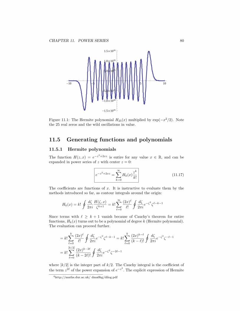
CHAPTER 11. POWER SERIES 80
-10 -5 5 10
-1.5´1016
-1.0´1016
-5.0´1015
5.0´1015
1.0´1016
1.5´1016
Figure 11.1: The Hermite polynomial H25(x) multiplied by exp(−x2/2). Notethe 25 real zeros and the wild oscillations in value.
11.5 Generating functions and polynomials
11.5.1 Hermite polynomials
The function H(z, x) = e−z2+2xz is entire for any value x ∈ R, and can beexpanded in power series of z with center z = 0:
e−z2+2xz =
∞∑k=0
Hk(x)zk
k!(11.17)
The coefficients are functions of x. It is instructive to evaluate them by themethods introduced so far, as contour integrals around the origin:
Hk(x) = k!
∮dζ
2πi
H(ζ, x)
ζk+1= k!
∞∑ℓ=0
(2x)ℓ
ℓ!
∮dζ
2πie−ζ2
ζℓ−k−1
Since terms with ℓ ≥ k + 1 vanish because of Cauchy’s theorem for entirefunctions, Hk(x) turns out to be a polynomial of degree k (Hermite polynomial).The evaluation can proceed further.
= k!k∑
ℓ=0
(2x)ℓ
ℓ!
∮dζ
2πie−ζ2
ζℓ−k−1 = k!k∑
ℓ=0
(2x)k−ℓ
(k − ℓ)!
∮dζ
2πie−ζ2
ζ−ℓ−1
= k!
[k/2]∑ℓ=0
(2x)k−2ℓ
(k − 2ℓ)!
∮dζ
2πie−ζ2
ζ−2ℓ−1
where [k/2] is the integer part of k/2. The Cauchy integral is the coefficient of
the term z2ℓ of the power expansion of e−z2
. The explicit expression of Hermite
4http://maths.dur.ac.uk/ dma0hg/dilog.pdf
CHAPTER 11. POWER SERIES 81
polynomials is obtained:
Hk(x) = k!
[k/2]∑ℓ=0
(2x)k−2ℓ (−1)ℓ
ℓ!(k − 2ℓ)!(11.18)
H(z, x) is the generating function of Hermite polynomials and encodes theiranalytic properties. We learn a lot from it with little effort:1) the change z to −z in (11.17) is compensated by x to −x, then Hermitepolynomials have definite parity: Hk(−x) = (−1)kHk(x).2) the identities ∂xH(z, x) = 2zH(z, x) and ∂zH(z, x) = 2(−z+x)H(z, x), whentranslated to the power series expansion5, give the recurrence relations
H ′k(x) = 2kHk−1(x), Hk+1(x) = 2xHk(x)− 2kHk−1(x) (11.19)
with initial conditions H0(x) = 1 and H1(x) = 2x that can be obtained bydirect expansion of H(z, x).3) the identity (2z∂z − 2x∂x + ∂2x)H(z, x) = 0 corresponds to the second orderequation (which has another non-polynomial independent solution)
H ′′k − 2xH ′
k + 2kHk = 0
4) Hermite polynomials can be evaluated by Rodrigues’ formula6:
Hk(x) =
[∂k
∂tkH(t, x)
]t=0
=
[ex
2 ∂k
∂tke−(t−x)2
]t=0
=(−1)kex2 dk
dxke−x2
(11.20)
5) The integral∫∞−∞ dx e−x2
Hk(x)Hj(x) is symmetric in k and j. We evaluateit for k ≥ j by using Rodriguez’s formula for Hk(x), and doing k integration byparts: ∫ ∞
−∞dx e−x2
Hk(x)Hj(x) = (−1)k∫ ∞
−∞dxHj(x)
dk
dxke−x2
=
∫ ∞
−∞dx e−x2 dk
dxkHj(x) = 2kk!
√π δjk (11.21)
because Hk(x) = 2kxk + . . . (use eq.11.19). This is the orthogonality propertyof Hermite polynomials.The Cauchy product H(z, x)H(z, y) = H(z
√2, x+y√
2) gives an interesting sum-
mation formula (by equating the coefficients of equal powers of z):
k∑ℓ=0
(k
ℓ
)Hℓ(x)Hk−ℓ(y) = 2k/2Hk
(x+ y√
2
)Exercise 11.5.1. Evaluate the Cauchy product of the exponential series fore−z2
and e2tz and obtain the absolutely convergent power series of the generatingfunction (11.17).
5Derivation of the series term by term is possible because it is uniformly convergent bothin z and x, in any compact set.
6Olinde Rodrigues (1795, 1851)
CHAPTER 11. POWER SERIES 82
11.5.2 Laguerre polynomials
The polynomials arise in the study of the radial Schrodinger equation for theHydrogen atom. Two different generating functions are (|z| < 1):
e−
xz
1− z
(1− z)α+1=
∞∑k=0
Lαk (x)z
k, (1 + z)αe−xz =∞∑k=0
Lα−kk (x)zk (11.22)
Notation: L0k(x) = Lk(x).
There are several other generating functions whose power series expansionyield special functions that are important in mathematical physics7. Some ex-amples are briefly presented below, some will be considered in the study oforthogonal polynomials (Chapter on Hilbert spaces).
11.5.3 Chebyshev polynomials (of the first kind)
The power series expansion in z = 0 of [(1 − zeiθ)(1 − ze−iθ)]−1 is easily doneby means of the geometric series. It gives:
1− z cos θ
1− 2z cos θ + z2=
∞∑k=0
zk cos(kθ), |z| < 1 (11.23)
With cos θ = x, the same identity becomes:
1− xz
1− 2xz + z2=
∞∑k=0
zk Tk(x), |z| < 1 (11.24)
with functions Tk(x). The identity (1−xz) = (1−2xz+z2)∑∞
k=0 Tk(x)zk gives
T0(z) = 1, T1(x) = x and the recurrence relation
0 = Tk(x)− 2xTk−1(x) + Tk−2(x).
It appears that Tk(x) is a polynomial of order k in x, and is the polynomialexpansion of cos(kθ) in x = cos θ. The k roots of Tk(x) are real and known, andbelong to the interval [−1, 1]. On this interval |Tk(x)| ≤ 1.Chebyshev polynomials share the unique and important property: among allmonic polynomials of degree k, the one that deviates the least from zero on[−1, 1] is the polynomial 2−k+1Tk(x).
Exercise 11.5.2. Study the Chebyshev polynomials of the second kind:
1
1− 2xz + z2=
∞∑k=0
Uk(x)zk, |z| < 1
7A beautiful little book on special functions is: N. N. Lebedev, Special functions and theirapplications, Dover Ed. A modern reference book is the NIST Handbook of MathematicalFunctions, Cambridge Univ. Press.
CHAPTER 11. POWER SERIES 83
11.5.4 Legendre polynomials
In his Recherches sur l’attraction des spheroides homogenes (1783), Adrien MarieLegendre introduced the important expansion in multipoles:
1
|r − R|=
1√R2 − 2Rr cos θ + r2
=1
R
∞∑ℓ=0
Pℓ(cos θ)( rR
)ℓ(11.25)
θ is the angle between the vectors, R > r, Pk(cos θ) is a Legendre polynomialof order k in cos θ. The generating function
P (z, cos θ) = (1− 2z cos θ + z2)−1/2 = (1− zeiθ)−1/2(1− ze−iθ)−1/2
is analytic in the disk |z| < 1, where the two factors can be expanded in thebinomial series. The coefficients of the Cauchy product are the Legendre func-tions:
1√1− 2z cos θ + z2
=∑n,m
(−1/2)mm!
(−1/2)nn!
ei(m−n)θzm+n
=∞∑k=0
zkPk(cos θ)
Pk(cos θ) =
k∑m=0
(−1/2)mm!
(−1/2)k−m
(k −m)!cos(2m− k)θ
As Pk is an expression of cos(nθ) with n = 0, . . . , k, it may be rewritten as apolynomial of order k in the variable cos θ. In the variable x, |x| ≤ 1, it is:
1√1− 2xz + z2
=∞∑k=0
zkPk(x) (11.26)
From the identities (1 − 2xz + z2)∂zP (z, x) = (−z + x)P (z, x) and (1 − 2xz +z2)∂xP (z, x) = zP (z, x) one derives recurrence relations for the polynomials.Several more properties may be obtained by the above illustrated methods.
11.5.5 The Hypergeometric series
Several functions of mathematical physics correspond to special choices of thereal parameters a, b and c = 0,−1,−2, . . . of the hypergeometric function, whichhas a simple definition as a power series:
F (a, b; c; z) =∞∑
n=0
anbncn
zn
n!= 1 +
ab
cz +
1
2!
a(a+ 1)b(b+ 1)
c(c+ 1)z2 + . . . (11.27)
Note that F (a, b; c; z) = F (b, a; c; z). The series F (−k, b; c, z) terminates, andis a polynomial of degree k in z. The hypergeometric series is convergent for|z| < 1 (ratio test).The hypergeometric function F (a, b; c; z) is a solution of the differential equation
z(z − 1)F ′′(z) + [c− (a+ b− 1)z]F ′(z)− abF (z) = 0
Exercise 11.5.3. Show that: ∂zF (a, b; c, z) =abc F (a+ 1, b+ 1; c+ 1; z).
CHAPTER 11. POWER SERIES 84
11.6 Differential Equations
Power series are an effective representation of solutions of linear differentialequations. The subject is vast, and we only illustrate it with a useful statementand an example.
Theorem 11.6.1. In the linear second order differential equation,
f ′′(z) + p(z)f ′(z) + q(z)f(z) = 0
if p(z) and q(z) are analytic on a disk |z| < R, then any solution of the equationis analytic on the same disk.
11.6.1 Airy’s equation
Airy’s equation occurs in the study of a quantum particle in a uniform electricfield8, WKB theory, radio waves. Although the equation has a real variable,and one looks for real solutions, as a general rule it is useful to study it in thecomplex plane:
f ′′(z)− zf(z) = 0 (11.28)
The previous theorem assures that the solutions are entire functions and admitan absolutely convergent power series representation f(z) =
∑k ckz
k. Airy’sequation
0 =∑k≥0
ck[k(k − 1)zk−2 − zk+1]
implies a recursion for the coefficients: k(k − 1)ck = 0 for k = 0, 1, 2 andk(k − 1)ck = ck−3, k ≥ 3. Therefore c0 and c1 are undetermined, while c2 = 0.Starting from c0 = 0 and c1 = 0 one obtains c3 = c0/(2 · 3), c6 = c3/(5 · 6),c9 = c6/(8 · 9) ... A good guess helps to obtain the expression for the generalcoefficient:
c3kc0
=1
3k(3k − 1) · · · 9 · 8 · 6 · 5 · 3 · 2=
(3k − 2) · · · 10 · 7 · 4 · 1(3k)!
= 3k
(3k)!
(k − 1 + 1
3
)· · ·(2 + 1
3
) (1 + 1
3
)13 = 3k
Γ(3k+1)
Γ(k+
13
)Γ(13
)With the aid of the triplication formula9 for Γ(3k + 1):
c3k = c02π
Γ(13
) 1
32k+1/2k! Γ(k+
23
)8The Hamiltonian for an electron in a uniform electric field E along the x axis is H =
p2/2m+ eEx. The eigenvalue equation is separable and for the x component is:
−ℏ2
2mu′′(x) + eExu(x) = λu(x)
The linear potential eEx equals the energy λ at x0 = λ/eE, therefore the classical motion isconfined in x ≤ x0. The problem has a natural length ℓ = ℏ2/3(meE)−1/3 and the rescalingx − x0 = ℓ s brings the eigenvalue equation to Airy’s form. For a field E = 1 keV/cm it isℓ ≈ 9 nm.
9Γ(3z) = 33z−1/2
2πΓ(z)Γ
(z + 1
3
)Γ(z + 2
3
)
CHAPTER 11. POWER SERIES 85
By an appropriate choice of c0 a solution is obtained:
f0(z) =∞∑k=0
z3k
9k k! Γ(k + 23 )
=1
Γ( 23 )
[1 +
z3
6+
z6
180+ . . .
]Another independent solution is obtained with the choice c0 = 0 and c1 = 0.Then c4 = c1/(4 · 3), c7 = c4/(7 · 6) ...
f1(z) =∞∑k=0
z3k+1
9k k! Γ(k + 43 )
=1
Γ(43 )
[z +
z4
12+
z7
504+ . . .
]The two series have infinite radius and are entire functions. The standardsolutions are the Airy functions of the first and second kind:
Ai(z) = 3−2/3f0(z)− 3−4/3f1(z), Bi(z) = 3−1/6f0(z) + 3−5/6f1(z)
For z = x (real) both functions are oscillatory for x ≪ 0; for x ≫ 0 thefunction Ai (x) decays to zero exponentially while Bi (x) grows exponentially(see: Carl M. Bender and Steven A. Orszag, Advanced Mathematical Methodsfor Scientists and Engineers, Springer; O. Vallee and M. Soares, Airy functionsand applications to physics, World Scientific 2004.)
Chapter 12
ANALYTICCONTINUATION
The power series representation of an analytic function implies that its zerosare isolated. This has important and unexpected consequences, as the powerfulconcept of analytic continuation. Some relevant theorems about analytic mapsare presented.
12.1 Zeros of analytic functions
Theorem 12.1.1. Let f(z) be analytic on a domain D.If f(a) = 0 at a point a ∈ D and f is not constant in a neighborhood of a, thenthere is a punctured disk D′(a, δ) where f(z) = 0.If f(z) = 0 on an open subset O in D, then f(z) = 0 on D.
Proof. If f is not constant in a disk centred in a, the function has a power seriescentred in a, with some finite radius of convergence. If the zero is of order k,the coefficient ck is nonzero and
f(z) = ck(z − a)k[1 +
ck+1
ck(z − a) + . . .
]= ck(z − a)kφ(z)
where φ(z) is analytic in the disk, and φ(a) = 1. Since φ(z) is continuous in a,∀ϵ ∃δ such that |φ(z)− 1| < ϵ, i.e. there is no zero of φ in D(a, δ), and there isno zero of f on the same disk with point a removed.Suppose that f is zero on an open connected set O ⊂ D. If O is different fromD, there is a point of ∂O where f = 0 and f is not constant in a disk centredin it. As this would contradict the afore sentence, f = 0 on D.
Corollary 12.1.2. An analytic function on D that vanishes on a disk in D, ora line in D, or a set of points with an accumulation point in D, is zero on thewhole set D. Two functions analytic on a domain D that take the same valueson a line, or a sequence of points with an accumulation point in D, coincide.
Example 12.1.3. The function sin(2z)− 2 sin z cos z is entire and vanishes onthe real axis, therefore sin(2z)− 2 sin z cos z = 0 ∀z ∈ C.
86
CHAPTER 12. ANALYTIC CONTINUATION 87
12.2 Analytic continuation
Suppose that f is an analytic function defined on a set D that contains at leasta convergent sequence of points and its limit point. If f is a function analyticon D such that D ⊂ D and f = f on D, then f is the analytic continuationof f to D.
Theorem 12.2.1. The analytic continuation of f to D is unique.
Proof. Suppose that f1 and f2 are two extensions. Then f1 − f2 is zero on D.This implies that f1 − f2 = 0 on the whole set D.
Suppose that f1 and f2 are analytic on D1 and D2, and f1 = f2 on D1 ∩ D2.If the intersection contains at least a convergent sequence of points, then thefunction f = f1 on D1 and f = f2 on D2 is analytic on D1 ∪D2.
Consider a series f(z) =∑
n an(z−a)n that converges in the disk |z−a| < R.If in the disk we fix a point b and expand f with center b, we may find a radiusR′ > R − |b − a| (the new disk leaks out of the first one). The two expansionscoincide on the intersection, and together describe a single analytic function fon the union of the two disks.
The following power series converges in the disk |z| < 1, but diverges at allpoints of the boundary |z| = 1. Then it cannot be continued analytically:
G(z) =
∞∑n=0
z2n
= z + z2 + z4 + z8 + z16 + . . .
The coefficients are 0 and 1, then Cauchy-Hadamard’s criterion gives radiusR = 1. The series clearly diverges at z = ±1. Note that G(z2) = G(z) − z,therefore the series is divergent also at z = ±i. Again: G(z4) = G(z) − z − z2
and the series G(z) diverges at the roots of z4 = 1. In this way one provesdivergence at all points z2
n
= 1 (n = 1, 2, . . . ); such points are dense in the unitcircle, which is a singular line for G(z).
12.3 Gamma function
The function was devised by Euler (1729) to extend the factorial from positiveintegers to real and complex numbers:
Γ(z) =
∫ ∞
0
ds e−s sz−1 Re z > 0 (12.1)
The meaning of sz is ez log s. Note that:
|Γ(z)| ≤∫ ∞
0
ds e−s|sz−1| = Γ(Rez)
To show that the Gamma function is holomorphic, let γ be an arbitrary closedpath in the domain Re z > 0. The double integrals can be exchanged:∮
γ
dz Γ(z) =
∫ ∞
0
ds e−s
∮γ
dz e(z−1) log s
CHAPTER 12. ANALYTIC CONTINUATION 88
The last integral is zero by Cauchy’s formula. Then Morera’s theorem assuresthat Γ(z) is holomorphic. The function Γ′(z) is holomorphic on the same do-main, and is related to the Digamma function (see sect.12.3.2).
For z = x > 0, integration by parts of (12.1) gives the typical property of thefactorial: Γ(x + 1) = xΓ(x). Since Γ(1) = 1, it is Γ(n + 1) = n!. The propertyremains valid in the complex domain: the function Γ(z + 1)− zΓ(z) is analyticand vanishes on the real axis, then it must vanish everywhere in its domain:
Γ(z + 1) = zΓ(z) (12.2)
Exercise 12.3.1. Show that Γ(12 ) =√π and Γ(n+ 1
2 ) =√π (2n)!
4nn! (Hint: makethe change s = t2 in Euler’s integral).
Exercise 12.3.2. Evaluate the volume V and the area A of the sphere of radiusr in Rn. (Hint: compare the integrals
∫dnx exp(−
∑x2k) in Cartesian and
spherical coordinates).
V =πn/2
Γ(1 + n2 )rn, A =
n
rV. (12.3)
Exercise 12.3.3. Euler’s Beta function. Evaluate the double Euler integralfor Γ(x)Γ(y), x > 0 and y > 0, by changing to squared integration variables andthen to polar coordinates, and prove the useful formula1
B(x, y) ≡∫ 1
0
dt tx−1(1− t)y−1 =Γ(x)Γ(y)
Γ(x+ y)(12.4)
Euler’s integral for the Gamma function is well defined for Rez > 0. How-ever, by splitting the range of integration in (12.1) into [0, 1] ∪ [1,∞), andintegrating on [0, 1] by series expansion, one obtains
Γ(z) =
∫ ∞
1
ds e−s sz−1 +∞∑k=0
(−1)k
k!
1
z + k(12.5)
This expression provides the analytic continuation of Γ to Re z ≤ 0. It showsthat Γ(z) is the sum of an entire and a meromorphic function with simple polesat −k with residue (−1)k/k!, k ∈ N. An alternative definition on the puncturedcomplex plane was obtained by Gauss (1811):
Γ(z) = limn→∞
nz n!
z(z + 1)(z + 2) · · · (z + n)z = 0,−1,−2, . . . (12.6)
Exercise 12.3.4. Evaluate the following integral, that links the two definitionsof the Gamma function:∫ n
0
ds sz−1(1− s
n
)n=
nzn!
z(z + 1) · · · (z + n)(12.7)
Hint: use integration by parts.
1Atle Selberg, winner of a Fields medal (with Laurent Schwartz, 1950) for his studieson prime numbers, obtained an important multi-dimensional extension of the Beta function(Selberg’s integral).
CHAPTER 12. ANALYTIC CONTINUATION 89
From Gauss’ formula one easily obtains the useful duplication formula (aswell as the triplication, or multiplication by n)
Γ(2z) =22z−1
√π
Γ(z)Γ(z + 1
2
)(12.8)
In 1854 Weierstrass gave a definition for the reciprocal of the Gamma function,which is an entire function:
1
Γ(z)= z eCz
∞∏m=1
[(1 +
z
m
)e−z/m
](12.9)
with Euler’s constant
C = limn→∞
[1 + 1
2 + . . .+ 1n − log n
]= 0.5772156... (12.10)
Another useful representation, by Hankel, is given in eq.(27.3.1). Several im-portant formulae may be proven by the appropriate representation.
Exercise 12.3.5. Prove the interesting formulae:∫ ∞
0
dttz−1
et − 1= Γ(z)ζ(z), Re z > 1, (12.11)∫ ∞
0
dttz−1
et + 1= (1− 21−z)Γ(z)ζ(z), Re z > 0. (12.12)
(Hint: multiply and divide by e−t and expand in geometric series).The formulae appear respectively in the theory of free bosons and free fermions.The second integral is an analytic extension of Riemann’s series ζ(z) from Rez > 1 to Re z > 0.
Exercise 12.3.6. Show that limz→0 z ζ(1− z) = −1.
12.3.1 Stirling’s formula
The well known formula for the growth of the factorial is a particular case ofStirling’s expansion for Γ(x+ 1), when x is real and large:
Γ(x+ 1) ≈√2πx ex(log x−1)
[1 + 1
12 x + 1288 x2 +O
(1x3
)](12.13)
Proof. Put s = xt in the integral:
Γ(x+ 1) =
∫ ∞
0
ds e−s+x log s = x ex log x
∫ ∞
0
dt e−x(t−log t)
For x≫ 1, the neighborhood of the minimum of the exponent contributes most.The minimum is at t = 1, with expansion t− log t = 1+ 1
2 (t−1)2− 13 (t−1)3+ . . .
Therefore:
Γ(x+ 1) = x ex log x−x
∫ ∞
−1
dt exp[−x(12 t
2 − 13 t
3 + 14 t
4 − . . .)]
=√x ex log x−x
∫ ∞
−√x
dt exp(− 1
2 t2 + 1
3√xt3 − 1
4x t4 + . . .
)=
√x ex log x−x
∫ ∞
−√x
dt e−12 t
2[1 + t3
3√x+ 1
x
(t6
18 − t4
4
)+ . . .
]The lower limit of integration is replaced by −∞, with exponentially small error;the first three terms of the asymptotics are obtained.
CHAPTER 12. ANALYTIC CONTINUATION 90
12.3.2 Digamma function
The logarithmic derivative of the Gamma function defines the Digamma func-tion:
ψ(z) =1
Γ(z)
dΓ(z)
dz=
1
Γ(z)
∫ ∞
0
ds e−ssz−1 log s (12.14)
with the main property:
ψ(z + 1) =1
z+ ψ(z).
For integer values it gives ψ(n+ 1) = 1n + · · ·+ 1
2 + 1+ ψ(1). The behaviour ofthe harmonic series (12.10) implies that, for large n: ψ(n)− ψ(1) ≈ logn+ C.Stirling’s formula gives the behaviour for large real x:
ψ(x+ 1) ≈ log x+1
2x− 1
12x2+ . . .
then, ψ(1) = −C. Euler’s constant (12.10) is deeply related to the properties ofRiemann’s zeta function2.
12.4 Analytic maps
Theorem 12.4.1 (Open mapping theorem). If f is non-constant and an-alytic on a domain D, the image of an open subset in D is open (the converseis obviously true because f is continuous.)
Proof. Consider an open subset O in D and a point a ∈ O. The functiong(z) = f(z) − f(a) vanishes in a; then there is a disk centred on a of radius δand contained in O where g(z) = 0 i.e. |f(z)− f(a)| > 0. This means that thepoint f(a) has a an open neighborhood of points contained in f(O).
Theorem 12.4.2 (Maximum principle theorem). If f is non-constant andanalytic on a domain D, the maximum of |f(z)| is attained at the boundary ∂D.
Proof. Suppose that |f | attains its maximum at an interior point z0 ∈ D, withimage w0 = f(z0). Then there is an open disk D(z0, r) centred in z0 and con-tained in D. Since the image of the disk is open (Open mapping theorem 12.4.1)and contains w0, there is a disk |w − w0| < r′ contained in f(D). Thereforethere is a point w with |w| > |w0|, and this contradicts the hypothesis.
If f(z) = 0 on D, the same theorem applies to the holomorphic function1/f to give the minimum principle: the minimum of |f(z)| is attained at theboundary of D.
Exercise 12.4.3. Find the maxima of | cosh z| in the square of vertices 0, π, π+iπ, iπ.
Proposition 12.4.4 (Schwarz’s Lemma). Suppose that f is holomorphic andmaps the open unit disk D into itself, f(D) ⊆ D, with f(0) = 0. Then
|f(z)| ≤ |z|, ∀z ∈ D.2a nice book is: J. Havil, Gamma, exploring Euler’s constant, Princeton Univ Press, 2003.
CHAPTER 12. ANALYTIC CONTINUATION 91
Proof. The function f(z)/z has a removable singularity in z = 0, and is holo-morphic in the disk with the value f ′(0) at z = 0. Since it gains the maximummodulus at the boundary, it is: |f(z)|/|z| ≤ 1. In particular |f ′(0)| ≤ 1.
If the map is a bijection of the unit disk and f ′(z) = 0 (f is a conformalmap), Schwarz’s lemma applies to the inverse map f−1 as well. Then f ′(0) = 1,and |f(z)| = 1 if |z| = 1. For such functions, the power expansion is: f(z) =z + a2z
2 + a3z3 + . . . . Bieberbach’s conjecture (1916) states that |an| < n for
all n. He only proved |a2| < 2. Loewner proved |a3| < 3 by means of Loewner’sdifferential equation. The conjecture was proven by de Branges in 1984.A limit case with real coefficients is the power expansion of Koebe’s function:
z + 2z2 + 3z3 + 4z4 + . . . = zd
dz(1 + z + z2 + . . .) =
z
(1− z)2
It maps univalently the unit disk to the w-plane with cut Re w < −1/4,Imw = 0. The cut is the image of the unit circle3.
Here are some pearls from the theory of analytic functions:
Theorem 12.4.5 (Bohr, 1914). If f(z) =∑∞
k=0 ckzk is analytic on the unit
disk, where |f(z)| < 1, then∑∞
k=0 |ckzk| < 1 on the disk |z| < 1/3. This radiusis the best possible.
Theorem 12.4.6 (Bloch, 1924). If f is analytic on the unit disk D with f(0) = 0and f ′(0) = 1 then there is a number B (Bohr’s constant) independent of f suchthat there is a subset Ω ⊂ D where f is one-to-one, and such that f(Ω) containsa disk of radius B. (B = 0.4469, arXiv:1702.01080)
Theorem 12.4.7 (MacDonald 1898, Whittaker 1935). The number of zeros ofa non-constant function f analytic in a region bounded by a contour |f(z)| = cexceeds by unity the number of zeros of f ′ in the same region. (arXiv:1702.03458)
Theorem 12.4.8 (Earle-Hamilton fixed point theorem). Let f be a holomorphicfunction on a bounded domain D, such that the distance between f(D) and C/Dis greater than a positive constant. Then f has a unique fixed point.
3A magnificent reference is: R. Roy, Sources in the development of mathematics, Cam-bridge, 2011.
Chapter 13
LAURENT SERIES
13.1 Laurent’s series of holomorphic functions
A Laurent series with center a is the bilateral sum∞∑
n=−∞cn(z − a)n =
∞∑n=0
cn(z − a)n +∞∑
n=1
c−n1
(z − a)n(13.1)
It exists if both one-sided series converge. The two series are respectively calledthe analytic and the principal parts of the series. The analytic part convergesabsolutely on a disk centred in a with radius R,
lim sup n√|cn(z − a)n| < 1, → |z − a| < R,
1
R= lim sup n
√|cn|
The principal part (negative powers) converges absolutely for
lim sup n√|c−n(z − a)−n| < 1, → |z − a| > r = lim sup n
√|c−n|
Therefore, the Laurent series is well defined in the annulus
A(a, r,R) = z : r < |z − a| < R.
If the inner radius is zero and the point a is avoided, the annulus is the punctureddisk D′(a,R) = D(a,R)/a.Exercise 13.1.1. Discuss the convergence of the Laurent series:
∞∑k=−∞
3−|k|zk,∞∑
k=−∞
zk
cosh(3k).
Remark 13.1.2. Because both the principal and the analytic parts are powerseries (in z−a and its reciprocal) that are convergent in the annulus, convergenceis absolute, and it is uniform in the closed annulus r(1+η) ≤ |z−a| ≤ R(1−η′)where η, η′ > 0 are finite. Thus a Laurent series can be integrated term by termon a path in the annulus. In particular, for a closed path encircling the pointa with index 1, the integral of the analytic part is zero, and the integral of theprincipal part is 2πi c−1: ∮
γ
f(z)dz = 2πi c−1 (13.2)
92
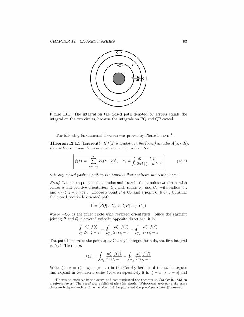
CHAPTER 13. LAURENT SERIES 93
P
−C_<
C_>
Q
.z
Figure 13.1: The integral on the closed path denoted by arrows equals theintegral on the two circles, because the integrals on PQ and QP cancel.
The following fundamental theorem was proven by Pierre Laurent1:
Theorem 13.1.3 (Laurent). If f(z) is analytic in the (open) annulus A(a, r,R),then it has a unique Laurent expansion in it, with center a:
f(z) =
∞∑k=−∞
ck(z − a)k, ck =
∮γ
dζ
2πi
f(ζ)
(ζ − a)k+1(13.3)
γ is any closed positive path in the annulus that encircles the center once.
Proof. Let z be a point in the annulus and draw in the annulus two circles withcenter a and positive orientation: C> with radius r> and C< with radius r<,and r< < |z − a| < r>. Choose a point P ∈ C< and a point Q ∈ C>. Considerthe closed positively oriented path
Γ = [PQ] ∪ C> ∪ [QP ] ∪ (−C<)
where −C< is the inner circle with reversed orientation. Since the segmentjoining P and Q is covered twice in opposite directions, it is:∮
Γ
dζ
2πi
f(ζ)
ζ − z=
∮C>
dζ
2πi
f(ζ)
ζ − z−∮C<
dζ
2πi
f(ζ)
ζ − z
The path Γ encircles the point z; by Cauchy’s integral formula, the first integralis f(z). Therefore:
f(z) =
∮C>
dζ
2πi
f(ζ)
ζ − z−∮C<
dζ
2πi
f(ζ)
ζ − z
Write ζ − z = (ζ − a) − (z − a) in the Cauchy kernels of the two integralsand expand in Geometric series (where respectively it is |ζ − a| > |z − a| and
1He was an engineer in the army, and communicated the theorem to Cauchy in 1843, ina private letter. The proof was published after his death. Weierstrass arrived to the sametheorem independently and, as he often did, he published the proof years later [Remmert]
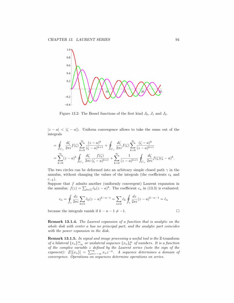
CHAPTER 13. LAURENT SERIES 94
5 10 15 20 25
-0.4
-0.2
0.2
0.4
0.6
0.8
1.0
Figure 13.2: The Bessel functions of the first kind J0, J1 and J2.
|z − a| < |ζ − a|). Uniform convergence allows to take the sums out of theintegrals
=
∮C>
dζ
2πif(ζ)
∞∑k=0
(z − a)k
(ζ − a)k+1+
∮C<
dζ
2πif(ζ)
∞∑k=0
(ζ − a)k
(z − a)k+1
=∞∑k=0
(z − a)k∮C>
dζ
2πi
f(ζ)
(ζ − a)k+1+
∞∑k=0
1
(z − a)k+1
∮C<
dζ
2πif(ζ)(ζ − a)k.
The two circles can be deformed into an arbitrary simple closed path γ in theannulus, without changing the values of the integrals (the coefficients ck andc−k).Suppose that f admits another (uniformly convergent) Laurent expansion inthe annulus: f(z) =
∑k∈Z ck(z − a)k. The coefficient cn in (13.3) is evaluated:
cn =
∮γ
dz
2πi
∑k∈Z
ck(z − a)k−n−1 =∑n∈Z
ck
∮γ
dz
2πi(z − a)k−n−1 = cn
because the integrals vanish if k − n− 1 = −1.
Remark 13.1.4. The Laurent expansion of a function that is analytic on thewhole disk with center a has no principal part, and the analytic part coincideswith the power expansion in the disk.
Remark 13.1.5. In signal and image processing a useful tool is the Z-transformof a bilateral xn∞−∞ or unilateral sequence xn∞0 of numbers. It is a functionof the complex variable z defined by the Laurent series (note the sign of theexponent): Z[xn] =
∑∞n=−∞ xnz
−n. A sequence determines a domain ofconvergence. Operations on sequences determine operations on series.
CHAPTER 13. LAURENT SERIES 95
13.2 Bessel functions (integer order)
The function J(z, x) = exp[ 12x(z − 1/z)] is analytic in the punctured complexplane C/0, where it has the Laurent expansion
exp
[x
2
(z − 1
z
)]=
∞∑k=−∞
zkJk(x) (13.4)
It is the generating function of Bessel’s functions of integer order, which arisein the study of Laplace’s operator in cylindrical coordinates2.A change of sign of z is compensated by a change of sign of x, J(−z, x) =J(z,−x), then Jk(−x) = (−1)kJk(x). The exchange of z with 1/z amountsagain to a change of sign of x, then J−k(x) = Jk(−x) = (−1)kJk(x). Fromthe expansion eix sin θ =
∑∞k=−∞ eikθJk(x), an integral expression for Bessel
functions is readily obtained:
Jk(x) =
∫ 2π
0
dθ
2πei(x sin θ−kθ) (13.5)
The generating function allows for a simple derivation of several properties.From ∂xJ(z, x) = 1
2 (z − 1/z)J(z, x) and z∂zJ(z, x) = x2 (z + 1/z)J(z, x) one
obtains
2J ′k(x) = Jk−1(x)− Jk+1(x),
2k
xJk(x) = Jk−1(x) + Jk+1(x) (13.6)
The two equations for J(z, x) also yield an equation where z and ∂z only appearin the combination z∂z: (z∂z)
2J(z, x) = (x2∂2x + x∂x + 1)J(z, x). The equationgives Bessel’s equation for integer order:[
d2
dx2+
1
x
d
dx+ 1− k2
x2
]Jk(x) = 0 (13.7)
Eq.(13.7) is written for another index, saym. Multiplicating the first by xJm(x)and the other by xJk(x) one obtains:
xd
dx(J ′
kJm − J ′mJk) + (J ′
kJm − J ′mJk)−
k2 −m2
xJkJm = 0
Now integrate in x on the positive reals. The first two terms cancel by integra-tion by parts (all Jk(x) decay as 1/
√x). The orthogonality property is:∫ ∞
0
dx
xJk(x)Jm(x) = 0 k = m (13.8)
Exercise 13.2.1. By expanding the integral representation (13.5) show thatJk(x) behaves as xk for small x (k ≥ 0).
Exercise 13.2.2. Write Helmholtz’s equation (∇2 + λ2)u = 0 in polar coor-dinates r, θ and separate it with functions u(r, θ) = R(r)Y (θ). Show how theradial equation becomes Bessel’s equation.
2Friedrich Wilhelm Bessel (1784, 1846) was the director of Konigsberg’s astronomical obser-vatory (Prussia) and measured the first stellar distance by parallax, after correctly interpretingthe apparent motion of 61 Cygni (discovered by Piazzi in Palermo) as due to Earth’s annualmotion. The same instrument (built by Fraunhofer) enabled him to discover the oscillationsof Sirius, due to an invisible companion star (a white dwarf) to be observed a century later.He developed an accurate theory for solar eclipses, and introduced Bessel’s function to solveKepler’s equation for planetary motion (see sect.20.3.2).
CHAPTER 13. LAURENT SERIES 96
13.3 Fourier series
Suppose that f is analytic in an annulus centred in the origin, that containsthe unit circle. In the annulus f has a Laurent expansion with coefficients fkevaluated as integrals on the unit circle. In particular, on the unit circle f theexpansion becomes:
f(eiθ) =
∞∑k=−∞
fk eikθ, fk =
∫ 2π
0
dθ
2πf(eiθ)e−ikθ
This Laurent’s expansion is the Fourier expansion of the 2π-periodic functionf(eiθ). It may be written in the form (with small change of notation):
f(θ) =∞∑
k=−∞
fk uk(θ), fk =
∫ 2π
0
dθ uk(θ) f(θ) (13.9)
where ukk∈Z is the Fourier basis of orthonormal 2π-periodic functions
uk(θ) =eikθ√2π,
∫ 2π
0
dθ um(θ)un(θ) = δmn (13.10)
The numbers fk are the Fourier coefficients of the periodic function f(θ).In this discussion f is the restriction of a holomorphic function to the unit circle,where it is continuous and differentiable. The problem of the minimal require-ments for a periodic function to admit a Fourier expansion will be consideredin section 20.1.
Chapter 14
THE RESIDUETHEOREM
14.1 Singularities.
Definition 14.1.1. When a function f(z) fails to be analytic at a point a, butis analytic in a punctured disk D′(a, r) = D(a, r)/a (a is removed from thedisk), the point a is an isolated singularity of f .
Example 14.1.2. The reciprocal 1/f of a holomorphic function has isolatedsingularities at the isolated zeros of f .
The Laurent expansion of the function in the punctured disk D′(a, r),
f(z) = . . .+c−k
(z − a)k+ · · ·+ c−1
z − a+ c0 + c1(z − a) + . . . ,
defines the principal and the analytic parts of f at its isolated singularity a.Since a punctured disk has inner radius equal to zero, the principal series existsat all points different from a, and converges uniformly on any compact set (forexample, on any bounded curve) that does not contain the singular point.
According to the principal part being null, terminating, or containing aninfinite number of terms, the singularity a is described by one of three types:
• The point a is a removable singularity if c−k = 0 for all k > 0.Example: f(z) = sin(z − a)/(z − a).
• The point a is a pole of order k if there is k > 0 such that c−k = 0 andc−k−n = 0 for all n > 0. It follows that limz→a(z − a)kf(z) = c−k.Example: f(z) = 1/(z − a)3 has a pole of order 3.
• The point a is an essential singularity if for any N there is k > N suchthat c−k = 0.Example: f(z) = exp[(z − a)−1]
Remark 14.1.3. There is a substantial difference between a pole and an es-sential singularity. If a is a pole for f , then limz→a f(z) = ∞. However, if ais an essential singularity, then limz→a f(z) is undefined. Indeed, a theorem byPicard states that if a is an essential singularity of f , the image f(D′) of thepunctured disk contains all complex points with at most one exception.
97
CHAPTER 14. THE RESIDUE THEOREM 98
Exercise 14.1.4. Study the behaviour of |1/z| and |e1/z| for z → 0.
Definition 14.1.5. A function is meromorphic on a domain D if it is analyticin D up to a set of isolated poles in D.
Theorem 14.1.6 (Picard’s little theorem for meromorphic function). Everyfunction meromorphic on C that omits three distinct complex values a, b and cis constant1.
14.2 Residues and their evaluation
Definition 14.2.1. The residue of a function f at the isolated singularity a isthe coefficient c−1 of the Laurent expansion in the punctured disk,
Res[f, a] = c−1 =
∮γ
dz
2πif(z) (14.1)
where γ is any (piecewise) smooth simple path encircling the singularity a an-ticlockwise inside the punctured disk of analyticity.
In view of their importance, we give rules to calculate residues that avoidthe evaluation of the contour integral.
• If f(z) has a simple pole in a (a pole of order 1), its Laurent expansion isf(z) = c−1(z − a)−1 + analytic part. Therefore the residue is
c−1 = limz→a
(z − a)f(z) (14.2)
• If f(z) has a pole of order k in a, it is (z − a)kf(z) = c−k + c−k+1(z −a) + · · ·+ c−1(z− a)k−1 + . . . . Then (k− 1) derivatives give (k− 1)!c−1+terms that vanish in z = a. The residue of f in a is
c−1 =1
(k − 1)!limz→a
dk−1
dzk−1
[(z − a)kf(z)
](14.3)
• If a is an essential singularity, the residue is computed with (14.1).
Example 14.2.2. In simple cases one may evaluate the residue by known ex-pansions. From e1/z = 1+1/z+ · · ·+1/(4!z4)+ . . . , it is Res [z3e1/z, 0] = 1/4!.Res [tan z/z5, 0] = 0 because the function is even, and its Laurent expansion inz = 0 only contains even powers.
Theorem 14.2.3 (The Residue Theorem ). Let f be an analytic function onD/S, where S = z1, . . . , zn is the set of its isolated singularities in the domainD. If γ is a closed piecewise smooth path in D/S such that Ind (γ, z) = 0 forall z /∈ D, then: ∮
γ
dζ f(ζ) = 2πin∑
k=1
Ind(γ, zk)Res[f, zk]. (14.4)
1see: R. Remmert, Classical topics in complex function theory, GTM 172, Springer 1998.
CHAPTER 14. THE RESIDUE THEOREM 99
Proof. Each singularity zk is the center of a punctured disk in D where f isanalytic and can be expanded in Laurent’s series: f(z) = Pk(z)+Ak(z). Whilethe analytic part Ak converges in the full disk, the principal part Pk convergesin C/zk.The function g(z) = f(z)−
∑k Pk(z) is analytic on D. By Cauchy’s theorem:
0 =
∮γ
dz g(z) =
∮γ
dz f(z)−∑k
∮γ
dz Pk(z)
The principal series can be integrated term by term because it converges uni-formly on γ. The integrals
∮γdz(z − zk)
−ℓ are zero for ℓ = 1; the integral ℓ = 1
is by definition 2πi Ind (γ, zk). Then∮γdz Pk(z) = 2πiRes[f, zk] Ind(γ, zk).
14.3 Evaluation of integrals
The Residue Theorem is a fundamental tool for evaluating integrals. In allapplications, one has to arrange the integral as an integral on a closed pathin the complex plane, either by a change of variable, or by closing the set ofintegration with extra curves. Usually, the method is successful if the integral onsuch additional curves is known (zero), or is proportional to the initial integral.The choice of the correct closed path is a matter of wisdom. However, somecases are typical and are here illustrated by examples.
14.3.1 Trigonometric integrals
Integrals in x ∈ [0, 2π] that only involve trigonometric functions may be attackedby writing the functions in terms of e±ix or powers, and putting z = eix. Thenew variable runs the unit circle C, and the Residue Theorem may apply.
Example 14.3.1.∫ 2π
0
dx1
2 + cosx=
∮C
dz
iz
2
4 + z + 1/z=
∮C
dz−2i
z2 + 4z + 1
The two roots z± = −2±√3 are simple poles, and |z+| < 1. Then:
= 2πi limz→z+
(z − z+)−2i
(z − z+)(z − z−)=
2π√3
Example 14.3.2.∫ 2π
0
dxcos(kx)
3 + sin2 x= Re
∫ 2π
0
dxeikx
3 + sin2 x= Re
∮C
dz
iz
4zk
12− (z − 1/z)2
= −4Re
∮C
dz
i
zk+1
(z2 − a)(z2 − 1/a)= π
(√7− 4
√3)k
2√3
[1 + (−1)k]
By taking the real part, one avoids the evaluation of two integrals. The poles±√a, with a = 7− 4
√3, are simple and in the unit disk.
CHAPTER 14. THE RESIDUE THEOREM 100
Exercise 14.3.3.∫ 2π
0
dθ
2π
cos(kθ)
cosh ξ − cos θ=
e−kξ
sinh ξ, ξ > 0, k = 0, 1, . . . (14.5)∫ 1
−1
dx√1− x2
1
y − x= π
sign(y)√y2 − 1
, |y| > 1 (14.6)∫ 2π
0
dxcos(2x)
1 + sin2 x= π(3
√2− 4) (14.7)
14.3.2 Integrals on the real line
Several integrals on the whole real line are attacked by closing the interval[−R,R] with a semicircle in the upper or lower half-plane and promoting thereal variable x to a complex variable z = x+ iy (then dz = dx on the real axis).If the Residue Theorem applies to the closed path γ, it provides the value ofthe integral if if the contribution of the semicircle vanishes in the limit R→ ∞.
Example 14.3.4.∫Rdx
x2
x4 + 1= lim
R→∞
∫ R
−R
dxx2
x4 + 1= lim
R→∞
∮γ
dzz2
z4 + 1
γ is the closed path [−R,R] ∪ z : z = Reiθ, 0 ≤ θ ≤ π. Since the functiondecays as R−2 in every direction, for R→ ∞ the contribution of the semicirclevanishes (Darboux’s inequality) (a semicircle in the lower half plane would beequally admissible). The path γ encircles the simple poles z1 = eiπ/4 and z2 =e3iπ/4. Then
= 2πi limz→z1
(z − z1)z2
(z4 + 1)+ 2πi lim
z→z2
(z − z2)z2
(z4 + 1)=
π√2
Remark 14.3.5. The asymptotic behaviour |f(Reiθ)|R → 0 as R → ∞ is asufficient condition for the integral on the semicircle to vanish.
There is an important class of integrals where the choice of half-plane is notfree, and the following result is useful:
Proposition 14.3.6 (Jordan’s lemma). Let f be a complex function, continuouson the semicircle σ = Reiθ, θ ∈ [0, π], and let M(R) = maxθ∈[0,π] |f(Reiθ)|.Then: ∣∣∣∣∫
σ
dzf(z)eiaz∣∣∣∣ ≤ π
aM(R), a > 0 (14.8)
Proof.∣∣∣∣∫σ
dzf(z)eiaz∣∣∣∣ = ∣∣∣∣iR ∫ π
0
eiθdθ f(Reiθ) eiaReiθ∣∣∣∣
≤ 2RM(R)
∫ π2
0
dθe−Ra sin θ ≤ 2RM(R)
∫ π2
0
dθe−2Raθ/π ≤ π
aM(R)
The inequality sin θ ≥ 2θ/π is used, for 0 ≤ θ ≤ π/2.If a < 0 the semicircle σ for convergence is in the lower half plane. In any casea = 0.
CHAPTER 14. THE RESIDUE THEOREM 101
If the maximum M(R) of |f | vanishes for R→ ∞, no matter how fast, thenthe semicircle contribution is zero. Here’s an important example:∫ ∞
−∞dx
e−ikx
x2 + a2=
π
ae−a|k|, a > 0, k ∈ R (14.9)
In the example, for k = 0 one is free to close in the upper or lower half plane.If k = 0, because e−ik(x+iy) must not blow up, one is compelled to close with asemicircle in the lower half plane if k > 0 or in the upper half plane if k < 0.
Example 14.3.7. Evaluate:∫ ∞
0
dxcos(kx)
(x2 + 1)2=π
4(|k|+ 1)e−|k| (14.10)
The function is even, then the integral is 1/2 the integral on the real axis;cos(kx) = Re exp(i|k|x). The path is closed in the upper half plane, whereit encircles the double pole z = i
=1
2Re 2πi lim
z→i
d
dz
[(z − i)2
ei|k|z
(z2 + 1)2
]= Re πi lim
z→i
d
dz
ei|k|z
(z + i)2= . . .
Exercise 14.3.8. ∫ ∞
0
dxx sin(πx)
(x2 + 1)2=π2
4e−π (14.11)
Ordinary integrals on the real line are tacitly defined with limits to infinitybeing taken independently:∫
Rf(x)dx = lim
u,v→∞
∫ v
−u
f(x)dx
The examples presented above use a weaker definition (Cauchy’s principal value):
P
∫Rf(x)dx = lim
R→∞
∫ R
−R
f(x)dx
where the limits are taken simultaneously. In several cases, the above principalvalue integrals are well defined as ordinary integrals.For an important class of integrals (Fourier integrals) the following statementholds:
Theorem 14.3.9 (Jordan). Let f(z) be analytic, save for isolated singularities.If a > 0 and if f(z) → 0 as z → ∞ in the upper half plane then:∫ ∞
−∞dx f(x) eiax = 2πi
n∑k=1
Res[f(z)eiaz, pk] (14.12)
where p1, . . . , pn are the singularities in the upper half plane.If a < 0 and f(z) → 0 as z → ∞ in the lower half plane, the sum involves thepoles in the lower half plane, with a change of sign.
CHAPTER 14. THE RESIDUE THEOREM 102
Proof. Consider the rectangular path with corners (−u, 0), (v, 0), (v, iw) and(−u, iw), u, v > 0, w = u + v. The rectangle is large enough to accomodateall singularities in the upper half plane. The integral of f(z)eiaz on this closedpath is 2πi times the sum of residues. Let us show that integration on all sidesbut the interval [−u, v] give zero for u, v → ∞: the integral on the segment fromv to v + iw is∣∣∣∣∫ w
0
idyf(v + iy)eiav−ay
∣∣∣∣ ≤ supy
|f(v + iy)|∫ w
0
e−ay ≤ 1
asupy
|f(v + iy)|,
the sup factor vanishes for v → ∞ (and u is left free). The opposite side behavessimilarly for u→ ∞ and all v. The integral on the side from −u+ iw to v+ iwis ∣∣∣∣∫ v
−u
dxf(x+ iw)eiax−aw
∣∣∣∣ ≤ e−aw(v + u) supx
|f(x+ iw)|,
and vanishes in the independent limits u and v → ∞.The integral on the whole real axis is obtained by two independent limits
limu→∞
∫ 0
−u
dx f(x)eiax + limv→∞
∫ v
0
dxf(x)eiax
and equals the integral on the closed rectangle.
14.3.3 Principal value integrals
When a real function has one or more simple poles on the real axis, we may stillgive meaning to the integral as a principal value integral (Cauchy), not to beconfused with the principal value integral on [−R,R], R→ ∞.This is an example: the integral
∫ c
a(x − b)−1 is singular, for a < b < c. How-
ever, one may isolate the singularity by removing an infinitesimal interval, andevaluate: ∫ b−ϵ
a
dx
x− b+
∫ c
b+η
dx
x− b= log
ϵ
b− a+ log
c− b
η
The independent limits ϵ, η → 0 do not give a well defined result. However, afinite result is obtained with the “principal value” prescription: ϵ = η, i.e. asymmetric interval, and ϵ→ 0. The result is:
−∫ c
a
dx
x− b= lim
ϵ→0
[∫ b−ϵ
a
dx
x− b+
∫ c
b+ϵ
dx
x− b
]= log
c− b
b− a(14.13)
In this section we evaluate principal value integrals on the whole real line asfollows:1) for each singularity ai of the real line remove a real interval [ai − ϵi, ai + ϵi];2) close the interval [−R,R] (R big enough to include all gaps) with a semicirclein the appropriate half-plane (we assume that for infinite radius the contribu-tion is zero);3) close each gap centred in the singularity ai by a semicircle of radius ϵi in thesame half plane as the big semicircle;4) the principal part integral (real axis with gaps) is the sum of two contribu-tions: the integral on the closed path (evaluated by residues) with R→ ∞, andthe integrals on the semicircles with opposite orientation (in order to cancel thecontributions that were added to close the contour) in the limits ϵi → 0.
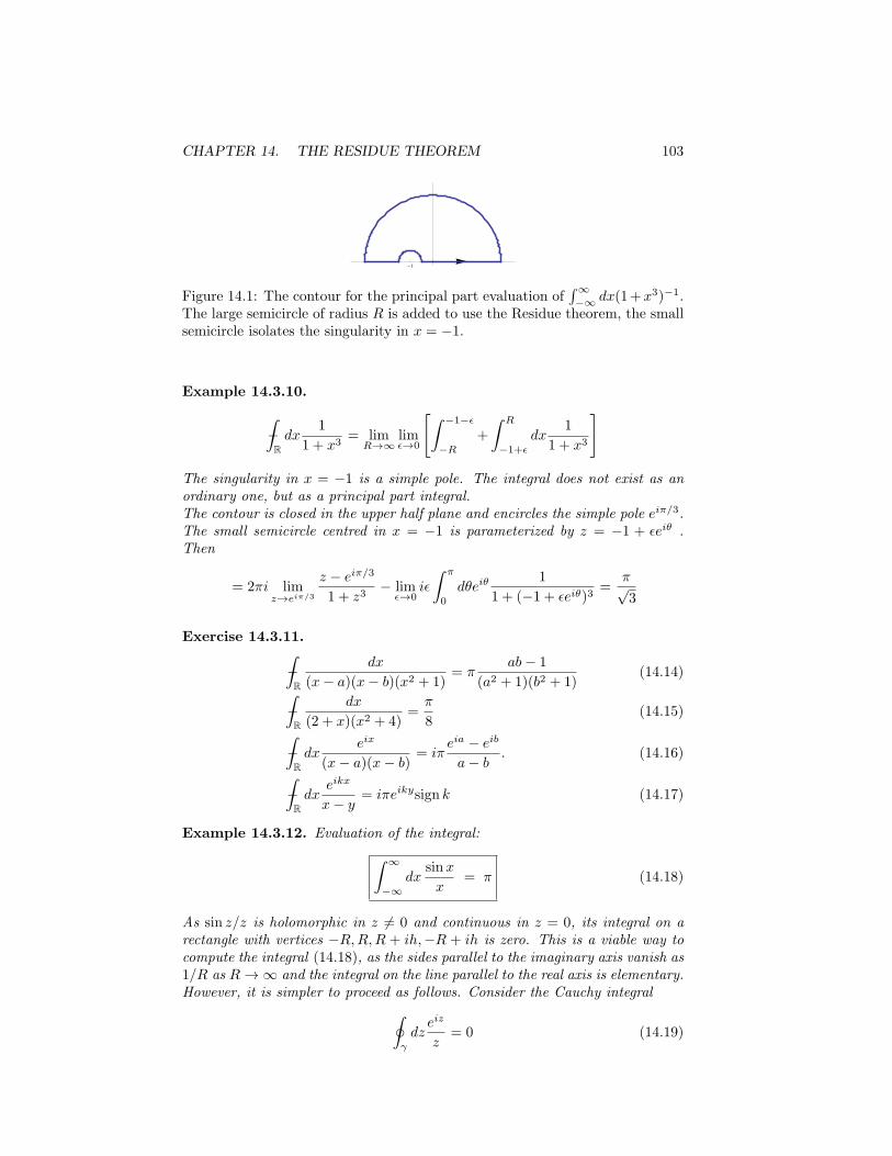
CHAPTER 14. THE RESIDUE THEOREM 103
-1
Figure 14.1: The contour for the principal part evaluation of∫∞−∞ dx(1+x3)−1.
The large semicircle of radius R is added to use the Residue theorem, the smallsemicircle isolates the singularity in x = −1.
Example 14.3.10.
−∫Rdx
1
1 + x3= lim
R→∞limϵ→0
[∫ −1−ϵ
−R
+
∫ R
−1+ϵ
dx1
1 + x3
]
The singularity in x = −1 is a simple pole. The integral does not exist as anordinary one, but as a principal part integral.The contour is closed in the upper half plane and encircles the simple pole eiπ/3.The small semicircle centred in x = −1 is parameterized by z = −1 + ϵeiθ .Then
= 2πi limz→eiπ/3
z − eiπ/3
1 + z3− lim
ϵ→0iϵ
∫ π
0
dθeiθ1
1 + (−1 + ϵeiθ)3=
π√3
Exercise 14.3.11.
−∫R
dx
(x− a)(x− b)(x2 + 1)= π
ab− 1
(a2 + 1)(b2 + 1)(14.14)
−∫R
dx
(2 + x)(x2 + 4)=π
8(14.15)
−∫Rdx
eix
(x− a)(x− b)= iπ
eia − eib
a− b. (14.16)
−∫Rdx
eikx
x− y= iπeikysign k (14.17)
Example 14.3.12. Evaluation of the integral:∫ ∞
−∞dx
sinx
x= π (14.18)
As sin z/z is holomorphic in z = 0 and continuous in z = 0, its integral on arectangle with vertices −R,R,R + ih,−R + ih is zero. This is a viable way tocompute the integral (14.18), as the sides parallel to the imaginary axis vanish as1/R as R→ ∞ and the integral on the line parallel to the real axis is elementary.However, it is simpler to proceed as follows. Consider the Cauchy integral∮
γ
dzeiz
z= 0 (14.19)
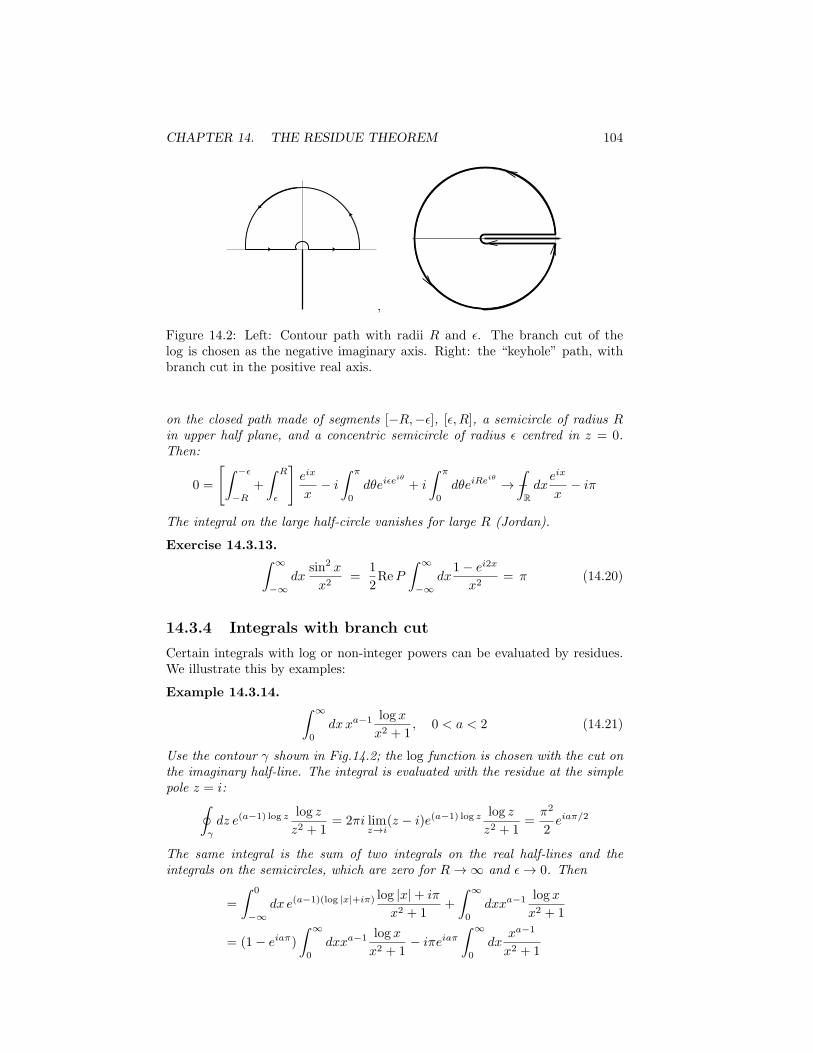
CHAPTER 14. THE RESIDUE THEOREM 104
,
Figure 14.2: Left: Contour path with radii R and ϵ. The branch cut of thelog is chosen as the negative imaginary axis. Right: the “keyhole” path, withbranch cut in the positive real axis.
on the closed path made of segments [−R,−ϵ], [ϵ, R], a semicircle of radius Rin upper half plane, and a concentric semicircle of radius ϵ centred in z = 0.Then:
0 =
[∫ −ϵ
−R
+
∫ R
ϵ
]eix
x− i
∫ π
0
dθeiϵeiθ
+ i
∫ π
0
dθeiReiθ → −∫Rdxeix
x− iπ
The integral on the large half-circle vanishes for large R (Jordan).
Exercise 14.3.13.∫ ∞
−∞dx
sin2 x
x2=
1
2ReP
∫ ∞
−∞dx
1− ei2x
x2= π (14.20)
14.3.4 Integrals with branch cut
Certain integrals with log or non-integer powers can be evaluated by residues.We illustrate this by examples:
Example 14.3.14. ∫ ∞
0
dxxa−1 log x
x2 + 1, 0 < a < 2 (14.21)
Use the contour γ shown in Fig.14.2; the log function is chosen with the cut onthe imaginary half-line. The integral is evaluated with the residue at the simplepole z = i:∮
γ
dz e(a−1) log z log z
z2 + 1= 2πi lim
z→i(z − i)e(a−1) log z log z
z2 + 1=π2
2eiaπ/2
The same integral is the sum of two integrals on the real half-lines and theintegrals on the semicircles, which are zero for R→ ∞ and ϵ→ 0. Then
=
∫ 0
−∞dx e(a−1)(log |x|+iπ) log |x|+ iπ
x2 + 1+
∫ ∞
0
dxxa−1 log x
x2 + 1
= (1− eiaπ)
∫ ∞
0
dxxa−1 log x
x2 + 1− iπeiaπ
∫ ∞
0
dxxa−1
x2 + 1
CHAPTER 14. THE RESIDUE THEOREM 105
Separation of real and imaginary parts gives two integrals:∫ ∞
0
dxxa−1
x2 + 1=
π
2 sin(aπ/2),
∫ ∞
0
dxxa−1
x2 + 1log x = −π
2
4
cos(πa/2)
sin2(πa/2)(14.22)
Example 14.3.15. ∫ ∞
0
dxxa−1 log x
x+ 1, 0 < a < 1 (14.23)
The path of the previous example does not help. The appropriate path is thekeyhole path (see Fig.14.2), with the log branch cut chosen as the real positivehalf-line. The integral is evaluated with the residue at the simple pole z = −1:∮
γ
dze(a−1) log z log z
z + 1= 2πi lim
z→−1(z + 1)e(a−1) log z log z
z + 1= 2π2eiaπ
The same integral is the sum of two integrals on two half-lines: the first one isjust above the branch cut (z = x + iϵ, arg z = 0), the second one is just belowthe branch cut and with opposite orientation (z = x − iϵ, arg z = i2π). Thelarge and small circles do not contribute. Then:
=
∫ ∞
0
dxxa−1 log x
x+ 1−∫ ∞
0
dx e(a−1)(log |x|+i2π) log |x|+ i2π
x+ 1
= (1− ei2aπ)
∫ ∞
0
dxxa−1 log x
x+ 1− i2πei2aπ
∫ ∞
0
dxxa−1
x+ 1
By separating real and imaginary parts we obtain two integrals:∫ ∞
0
dxxa−1
x+ 1=
π
sin(aπ),
∫ ∞
0
dxxa−1
x+ 1log x = −π2 cos(πa)
sin2(πa)(14.24)
Note that the integral with the log (and higher powers of the log) may be obtainedby a derivative in the parameter a of the first integral.
Exercise 14.3.16.
1)
∫ ∞
0
dx
√x
x3 + 1=π
3,
∫ ∞
0
dxx−1/3
x2 + a2=
π√3a−4/3 (a > 0) (14.25)
2)
∫ ∞
0
dxx−1/3
x2 + a2cos(kx) =
π√3a−4/3 cosh(ka), k ∈ R (14.26)
3)
∫ ∞
0
dxx−1/3
x2 + a2sin(kx) = πa−4/3 sinh(ka), k ∈ R (14.27)
4)
∫ ∞
0
dxx−1/3
x+ 1=
2π√3,
∫ ∞
0
dxx3/4
(x+ 1)3=
3√2
32π (14.28)
5)
∫ ∞
0
dxx1/4
(x+ 1)2=
π
2√2,
∫ ∞
0
dxx−1/n
(x+ 1)2=
π/n
sin(π/n)(14.29)
6)
∫ ∞
0
dx
√x
x3 + x2 + x+ 1=π
2(√2− 1) (14.30)
7)
∫ ∞
0
dxxµ
x2 − 2x cos θ + 1= π
sinµ(π − θ)
sin θ sin(µπ), |µ| < 1. (14.31)
Integrals 2,3: first evaluate the integral with exp(ikx), then separate even/oddpowers of k.
CHAPTER 14. THE RESIDUE THEOREM 106
14.3.5 Integrals of hyperbolic functions
The exponential and the hyperbolic functions are periodic on the imaginaryaxis, so the trick of closing [−R,R] with a semicircle at infinity does not work(the extra integral does not vanish). One rather exploits periodicity to close thepath by a rectangle, such that the function on the new side [−R+ ih,R+ ih] hasa simple relation with the function on the real interval. The trick was used forthe Fourier transform of the Gaussian function, (8.2). Here is another example:
Example 14.3.17. ∫Rdx
cos(xy)
coshx=
π
cosh(π2 y)(14.32)
The integral on [−R,R] is closed by the rectangle with vertices (±R, 0), (±R, iπ),where cosh(x + iπ) = − coshx and the integrals on the short sides vanish forR→ ∞. The rectangle encloses the simple pole iπ/2. Therefore:
2πi limz→iπ
2
(z − i
π
2
) cos(zy)
cosh z=
∫Rdx
cosxy
coshx−∫Rdx
cos y(x+ iπ)
cosh(x+ iπ)
Exercise 14.3.18. ∫ ∞
0
dxcos(xy)
cosh2 x=
πy/2
sinh(πy/2)(14.33)
Example 14.3.19.∫ ∞
−∞dk
sinh(ky)
sinh keikx =
π sin(πy)
cosh(πx) + cos(πy)(0 < y < 1). (14.34)
The integral, with a change k → −k, becomes:∫ ∞
−∞
dk
2
[ek(y+ix)
sinh k+ek(y−ix)
sinh k
]= Re−
∫ ∞
−∞dk
ek(y+ix)
sinh k.
Since sinh(z + iπ) = − sinh z, one considers a rectangle with corners −u, v,v + iπ, −u+ iπ, where u, v → ∞. Two sides are deformed by small half-circlesof radius ϵ to exclude the singular points k = 0, iπ from the interior of therectangle. By Cauchy’s formula the loop-integral is zero, and the integrals onthe sides parallel to the imaginary axis vanish in the limit. Then:
0 =[1 + eiπ(y+ix)
]−∫ ∞
−∞dkek(y+ix)
sinh k−∫ π
0
iϵeiθdθeϵe
iθ(y+ix)
sinh(ϵeiθ)
−∫ 2π
π
iϵeiθdθe(iπ+ϵeiθ)(y+ix)
sinh(iπ + ϵeiθ)
Therefore:
−∫ ∞
−∞dk
ek(y+ix)
sinh k= iπ
eπx − eiπy
eπx + eiπy(14.35)
The real part gives the integral.
CHAPTER 14. THE RESIDUE THEOREM 107
14.3.6 Other examples
Example 14.3.20.∫ ∞
0
dx1
x5 + 1=
π/5
sin(π/5),
∫ ∞
0
dxlog x
x5 + 1= −
(π5
)2 cos(π/5)
sin2(π/5)(14.36)
The denominator remains unchanged if x is replaced by z = xei2π/5. Thissuggests to close the real positive line with an arc of amplitude 2π/5 and theradial line z = xei2π/5 (the second integral requires the first one).
Example 14.3.21. ∫ ∞
0
dxlog x
x2 − 1=π2
4(14.37)
The cut is chosen away from the real positive axis, and the point x = 1 is aremovable singularity. If x is replaced by ix the integral is simple to evaluate.Theferore, integrate on the closed path formed by [0, R], the circle Reiθ 0 < θ <π2 and the segment [iR, 0], R→ ∞.
Example 14.3.22. ∫ ∞
0
dxlog(x2 + 1)
x2 + 1= π log 2 (14.38)
Evaluate∮γdz log(z+i)/(z2+1) where γ is the real axis closed by a semicircle in
the upper half plane. The cut of log(z+ i) is any line connecting −i to infinity,for example the line [−i,−i∞).
Example 14.3.23.∫ ∞
0
dxlog x
(x+ a)(x+ b)=
1
2
(log b)2 − (log a)2
b− a(14.39)
If the keyhole path is considered, the integral is cancelled by the integral onthe other side of the cut. The trick here is to evaluate the keyhole integral ofthe function (log z)2/(z + a)(z + b) (see P. Nahin, Inside interesting integrals,Springer 2015).
The Mathematics Stack Exchange is a website devoted to questions and an-swers at any level. In particular the following pages contain hundreds of ques-tions on contour integralshttp://math.stackexchange.com/questions/tagged/contour-integration
14.4 Enumeration of zeros and poles
Theorem 14.4.1. Let f(z) be meromorphic in D and γ a Jordan curve in D.If z1, . . . , zn are the zeros (of order k1, . . . , kn) and p1, . . . pm are the poles (oforder q1, . . . , qm) of f encircled by γ, then:∮
γ
dz
2πi
f ′(z)
f(z)=∑i
ki −∑j
qj . (14.40)
CHAPTER 14. THE RESIDUE THEOREM 108
Proof. A zero or a pole of f is a pole for f ′/f . In a neighbourhood of a zero zi,f(z) = Ai(z − zi)
kiφi(z) with φi analytic. Then
f ′(z)
f(z)=
ki(z − zi)
+φ′i(z)
φi(z)
with residue ki. In a neighbourhood of a pole, f(z) = (z − pj)−qjϕj(z) with ϕj
analytic. Thenf ′(z)
f(z)=
−qj(z − pj)
+ϕ′j(z)
ϕj(z)
and the residue is −qj . The integral is the sum of the residues of all zeros andsingular points encircled by γ.
Exercise 14.4.2. Show that:∫|z|=kπ
dz2πi tan z = −2k.
This beautiful theorem is useful for studying the location of zeros of analyticfunctions:
Theorem 14.4.3 (Rouche). Lef f and g be holomorphic functions on and insidea simple closed curve γ. If |g(z)| < |f(z)| for all z ∈ γ, then f and f + g havethe same number of zeros inside γ.
Proof. Since |f | > |g| on γ it is |f | = 0 on γ and the variable w = [f(z) +g(z)]/f(z) is well defined on γ. By the inequality |w(z) − 1| < 1, z ∈ γ, theimage of the curve γ does not encircle the origin. By eq.(14.40)
#(zeros of f + g)−#(zeros of f) =
∮γ
dz
2πi
w′(z)
w(z)=
∆arg w
2π= 0
(the zeros and poles of w are respectively the zeros of f + g and of f).
Example 14.4.4. How many solutions of ez − 3z4 + 5z = 0 are in the disk|z| < 2? Choose f(z) = −3z4 + 5z and g(z) = ez. On the boundary |g(z)| =e2 cos θ, |f(z)| = |48e4iθ − 10eiθ| > 38. Since |f | > |g|, the number of solutionsequals that of 3z4 − 5z = 0 in |z| < 2, which is 4.
14.5 Evaluation of sums
The theorem of residues can be used to evaluate infinite sums by reducing themto sums on a finite number of residues.The functions π cot(πz) and πcosec(πz) are meromorphic with simple poles onthe real axis at zn = n ∈ Z, and residues respectively equal to 1 and (−1)n. Iff(z) is analytic in the neighbourhood of the integer n, then:
Res[f(z)π cot(πz), n] = f(n), Res[f(z)πcosec(πz), n] = (−1)nf(n).
Proposition 14.5.1. Let f(z) be meromorphic with a finite set of poles P =p1, . . . , pm and suppose that there is K > 0 such that |z2f(z)| < K for all zwith |z| larger than some constant R. Then
0 =∑
n∈Z/P
f(n) +n∑
k=1
Res [f(z)π cot(πz), pk] (14.41)
0 =∑
n∈Z/P
(−1)nf(n) +
m∑k=1
Res [f(z)πcosec(πz), pk] (14.42)
CHAPTER 14. THE RESIDUE THEOREM 109
Proof. To apply the theorem of residues, consider a square path with corners±[n+ 1
2 ± i(n+ 12 ] big enough to include all poles pk. Then:∮
dζ
2πif(ζ)g(ζ) =
∑a
Res[f(z)g(z), a]
where a ∈ 0,±1, . . . ,±n∪p1, . . . pm, and g(z) is either π cot(πz) or πcosec(πz).On the sides of the squares it is | cot(πz)| ≤ 1 and |cosec(πz)| < 1. Then Dar-boux’s inequality and the bound on f ensure that the contour integral vanishesfor n→ ∞: ∣∣∣∣∮ dζ
2πif(ζ)g(ζ)
∣∣∣∣ ≤ 4(2n+ 1)
2π
K
(n+ 1/2)2
Corollary 14.5.2. If f is meromorphic with poles in p1, . . . , pk /∈ Z, then
∞∑n=−∞
f(n) = −m∑
k=1
Res [f(z)π cot(πz), pk] (14.43)
∞∑n=−∞
(−1)nf(n) = −m∑
k=1
Res [f(z)πcosec(πz), pk] (14.44)
Example 14.5.3. The function f(ζ) = 1/(ζ2+ z2) has simple poles ±iz. Then∑∞n=−∞
1n2+z2 =
∑p=±iz Res[
π cot(πζ)ζ2+z2 , p] = π
z coth(πz). One obtains a repre-
sentation for coth(πz):
coth(πz) =1
πz+ 2
z
π
∞∑n=1
1
z2 + n2(14.45)
For |z| < 1 one may expand as a geometric series: 1n2+z2 =
∑ℓ(−1)ℓ z2ℓ
n2+2ℓ . Theexchange of sums is allowed because the series are absolutely convergent:
coth(πz) =1
πz+
2
π
∞∑ℓ=0
(−1)ℓz2ℓ+1ζ(2 + 2ℓ) (14.46)
Comparison with eq.(11.13) reveals the relationship of zeta at even integers withBernoulli numbers:
ζ(2ℓ) =1
2
(2π)2ℓ
(2ℓ)!|B2ℓ| (14.47)
The replacement z → iz gives:
cot(πz) =1
πz+ 2
z
π
∞∑n=1
1
z2 − n2. (14.48)
As cot(πz) = 1π
ddz log sin(πz) and 2z
z2−n2 = ddz log(z
2 − n2), the famous productformula for the sine function results (Euler, 1734):
sin(πz) = πz∞∏
n=1
(1− z2
n2
)(14.49)
CHAPTER 14. THE RESIDUE THEOREM 110
Example 14.5.4. Consider f(z) = z−2, with a double pole at the origin.∑n=0 n
−2 = −Res[π cot(πz)z2 , 0]. The residue is evaluated with the rule for poles
of order 3:
2ζ(2) = − 1
2!limz→0
d2
dz2πz cos(πz)
sin(πz)
A different way to evaluate the residue is to produce the Laurent series directly,
from known series, and read c−1:π cos(πz)z2 sin(πz) =
π[1−(πz)2/2!+... ]z3π[1−(πz)2/3!+...] =
1z3 − π2
3z + . . . .
Then c−1 = −π2/3 and
ζ(2) =∞∑
n=1
1
n2=π2
6
Chapter 15
ELLIPTIC FUNCTIONS
15.1 Elliptic integrals I
Elliptic integrals are of the sort∫dxR
(x,√p3,4(x)
)where R is a rational func-
tion of the real variable x and of the square root of a cubic or quartic polyno-mial with real coefficients (a higher degree defines hyperelliptic integrals). Earlystudies were done by Fagnano, Euler, Lagrange and Landen. Legendre showedthat any elliptic integral may be expressed as a combination of three canonicalelliptic integrals.
The canonical elliptic integrals of the first kind arise in the study of thependulum. Let φ be the angular coordinate of the pendulum of length ℓ, φ0 themaximal deviation. Energy conservation gives: 1
2ℓ2φ2 = gℓ(cosφ − cosφ0) =
2gℓ(sin2(φ0/2) − sin2(φ/2)) (g is the gravitational acceleration). The time toswing from 0 to φ is:
t(φ) =1
2
√ℓ
g
∫ φ
0
dφ′√sin2(φ0/2)− sin2(φ′/2)
,
The period of the pendulum is T = 4t(φ0). With the change of variablesin(φ/2) = k sin θ, with parameter k = sin(φ0/2), they become t =
√ℓ/gF (θ, k)
and T = 4√ℓ/gK(k), where F (θ, k) = F (u|k) and K(k) = F (π2 , k) = F (1|k)
are respectively the incomplete and the complete elliptic integrals of the firstkind:
F (θ, k) =
∫ θ
0
dθ′1√
1− k2 sin2 θ′(15.1)
=
∫ u
0
dx√(1− x2)(1− k2x2)
= F (u|k) (15.2)
K(k) =
∫ π/2
0
dθ′1√
1− k2 sin2 θ′=
∫ 1
0
dx√(1− x2)(1− k2x2)
(15.3)
The archetypal elliptic integrals of the second kind arise in the eval-uation of the arc-length of the ellipse. Let the length of the semi-major axisbe one, and the eccentricity be k. The ellipse has parameterization x = cos θ,
111
CHAPTER 15. ELLIPTIC FUNCTIONS 112
y =√1− k2 sin θ. Then ds2 = dx2 + dy2 = (1 − k2 cos2 θ)dθ. The integral for
the arc-length∫ θ
0dθ′
√1− k2 cos2 θ′ can be expressed as E(π2 , k)−E(π2 − θ, k),
where
E(θ, k) =
∫ θ
0
dθ′√1− k2 sin2 θ′ (15.4)
=
∫ u
0
dx
√1− k2x2
1− x2= E(u|k), (15.5)
E(k) =
∫ π/2
0
dθ′√1− k2 sin2 θ′ =
∫ 1
0
dx
√1− k2x2
1− x2. (15.6)
E(θ, k) or E(u|k) are different notations for the incomplete elliptic integral ofthe second kind. E(k) = E(π2 , k) = E(1|k) is the complete elliptic integral ofthe second kind1. In this example, the perimeter of the ellipse is 4E(k).
Finally, the incomplete elliptic integral of the third kind is:
Π(θ, α, k) =
∫ θ
0
dθ′1
(1 + α2 sin2 θ′)√
1− k2 sin2 θ′(15.7)
=
∫ u
0
dx
(1 + α2x2)√
(1− x2)(1− k2x2)= Π(u|α, k) (15.8)
In these integrals, the number 0 ≤ k < 1 is the modulus. One also defines thecomplementary modulus k′ =
√1− k2.
The complete elliptic integrals K, E, K ′ ≡ K(k′) and E′ ≡ E(k′) are linkedby Legendre’s relation:
KE′ +K ′E −KK ′ =π
2(15.9)
Exercise 15.1.1. Show that
KE′ +K ′E −KK ′ =
∫ π2
0
dθ
∫ π2
0
dθ′k2 cos2 θ + k′
2cos2 θ′√
(1− k2 sin2 θ)(1− k′2 sin2 θ′)
The reduction of simple elliptic integrals to linear combinations of the canon-ical Legendre integrals is found in the tables of integrals, and the values ofLegendre integrals are tabulated2.
Example 15.1.2.∫ x
a
dx′√(x′ − a)(b− x′)(c− x′)
=2√c− a
F
(θ,
√b− a
c− a
), sin2 θ =
x− a
b− a
where a ≤ x ≤ b < c. The Legendre form is obtained with the replacement
1here and later, the same symbols E, F etc. are used whether the variable is θ or u = sin θ.Note the different separator of the arguments.
2A specialized book is P. F. Byrd and M. D. Friedman, Handbook of Elliptic Integrals forEngineers and Scientists, 2nd ed. 1971, Springer-Verlag.
CHAPTER 15. ELLIPTIC FUNCTIONS 113
x′ = a+ (b− a) sin2 θ′. Then x = a+ (b− a) sin2 θ. Similarly:∫ x
a
x′ dx′√(x′ − a)(b− x′)(c− x′)
=
∫ x
a
dx′
[c√
(x′ − a)(b− x′)(c− x′)−
√c− x′
(x′ − a)(b− x′)
]
=2c√c− a
F
(θ,
√b− a
c− a
)− 2
√c− aE
(θ,
√b− a
c− a
)Exercise 15.1.3. ∫ 1
0
dx√1− x4
= 1√2K(
1√2
)The integral is also amenable to Euler’s Beta function, 1
4B( 14 ,12 ). Show that:
K(
1√2
)=
1
4√πΓ(14 )
2.
Exercise 15.1.4. Find the first correction to the isochronous period of thependulum, in the small parameter φ0.
Exercise 15.1.5. Show that (from Bowman. Put t = tan θ)∫ x
0
dt√t4 ± 2t2 cosφ+ 1
=
∫ θ
0
dθ′√1− 1
2 (1∓ cosφ) sin2(2θ′)
=1
2F
(2 arctg x,
√1∓ cosφ
2
)(15.10)
∫ ∞
0
dt√t4 ± 2t2 cosφ+ 1
=2
∫ 1
0
dt√t4 ± 2t2 cosφ+ 1
=K
(√1∓ cosφ
2
)(15.11)
Exercise 15.1.6. Use the results of the previous exercise to prove the following(hint: 1− t = s2 or t− 1 = s2):∫ x
1
dt√t3 − 1
=14√3F
(2θ,
√3− 1
2√2
), cos(2θ) =
√3 + 1− x√3− 1 + x
(15.12)
∫ ∞
1
dt√t3 − 1
=24√3K
(√3− 1
2√2
), (15.13)
∫ 1
0
dt√1− t3
=14√3F
(2θ,
√3− 1
2√2
), cos(2θ) = 2−
√3 (15.14)
The last integral is also Beta Euler’s function: 13B( 13 ,
12 )
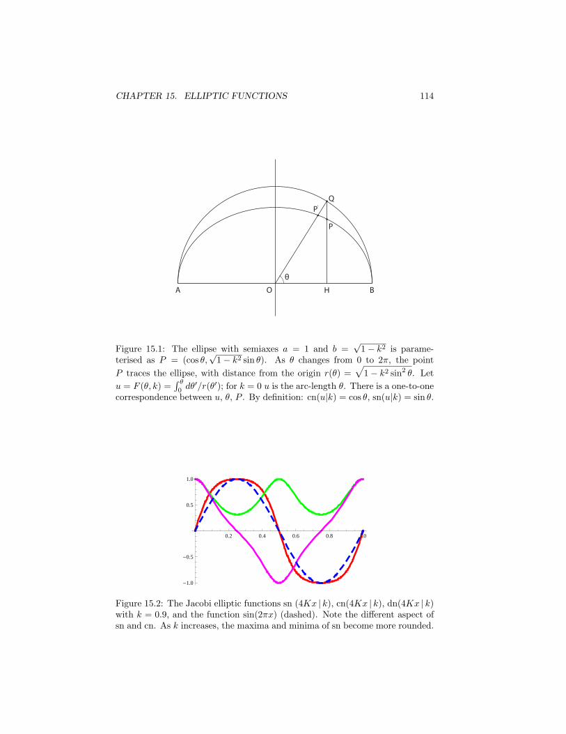
CHAPTER 15. ELLIPTIC FUNCTIONS 114
A BH
P
Q
O
P
Figure 15.1: The ellipse with semiaxes a = 1 and b =√1− k2 is parame-
terised as P = (cos θ,√1− k2 sin θ). As θ changes from 0 to 2π, the point
P traces the ellipse, with distance from the origin r(θ) =√
1− k2 sin2 θ. Let
u = F (θ, k) =∫ θ
0dθ′/r(θ′); for k = 0 u is the arc-length θ. There is a one-to-one
correspondence between u, θ, P . By definition: cn(u|k) = cos θ, sn(u|k) = sin θ.
0.2 0.4 0.6 0.8 1.0
-1.0
-0.5
0.5
1.0
Figure 15.2: The Jacobi elliptic functions sn (4Kx | k), cn(4Kx | k), dn(4Kx | k)with k = 0.9, and the function sin(2πx) (dashed). Note the different aspect ofsn and cn. As k increases, the maxima and minima of sn become more rounded.
CHAPTER 15. ELLIPTIC FUNCTIONS 115
15.2 Jacobi elliptic functions
The elliptic integral of the first kind F (θ, k) with modulus 0 ≤ k < 1 is amonotonic odd function of θ in the interval [−π
2 ,π2 ], with range [−K,K]. There
is no obstacle in letting θ vary on real axis. The addition formula suffices:
F (θ + π, k) =
∫ π
0
+
∫ π+θ
π
dθ′1√
1− k2 sin2 θ′= 2K + F (θ, k).
The extended function is non-decreasing, and so it is invertible. For k = 0, ifu = F (θ, 0), then sinu = sin θ. For k = 0 one defines a new function sn(u|k)that generalizes the sine function (Cayley named it ”the elliptic sine”)3:
u = F (θ|k), sn(u|k) = sin θ (15.15)
The function is odd in u, with extremal values sn(±K|k) = ±1. Since F (θ +π, k) = x+ 2K, it is
sn(u+ 2K|k) = sin(θ + π) = − sin θ = −sn(u|k) (15.16)
Then sn(u|k) is 4K-periodic. Next, it is natural to introduce the 4K-periodiceven function cn(u|k) = cos θ. Then:
cn2(u|k) + sn2(u|k) = 1 (15.17)
A function with no trigonometric counterpart, with period 2K, is:
dn(u|k) =√1− k2 sn2(u|k) (15.18)
sn, cn, dn are the Jacobian elliptic functions.
15.2.1 Derivatives
The relations du = dθ(1− k2 sin2 θ)−1/2 and d sn(u|k) = cos θ dθ allow to eval-uate the derivatives:
d
dusn(u|k) = cos θ
√1− k2 sin2 θ = cn(u|k) dn(u|k) (15.19)
d
ducn(u|k) =− sin θ
√1− k2 sin2 θ = −sn(u|k) dn(u|k) (15.20)
d
dudn(u|k) =− k2sn(u|k) cn(u|k) (15.21)
They imply the second-order differential equations:
d2
du2sn(u|k) =− (1 + k2) sn(u|k) + 2k2sn3(u|k) (15.22)
d2
du2cn(u|k) =− (1− 2k2) cn(u|k)− 2k2cn3(u|k) (15.23)
d2
du2dn(u|k) = (2− k2) dn(u|k)− 2 dn3(u|k) (15.24)
3Refs: F. Bowman, Introduction to Elliptic Functions with applications, Dover 1961;J. V. Armitage and W. F. Eberlein, Elliptic Functions, London Math. Soc. Student text67, Cambridge 2006.
CHAPTER 15. ELLIPTIC FUNCTIONS 116
Other equations are obtained by squaring the first derivatives; for example:[d
dusn(u|k)
]2= 1− (1 + k2)sn2(u|k) + k2sn4(u|k) (15.25)
15.2.2 Summation formulae
The Jacobi elliptic functions obey summation formulae. Let s1(x) = sn(x +x1|k), s2(x) = sn(x+x2|k), and the like for the other Jacobi functions. A primedenotes a derivative in x. Multiply (15.22) for s1 by s2, and subtract from itthe equation with labels exchanged:
(s2s′1 − s1s
′2)
′ = 2k2s1s2(s21 − s22)
Multiply (15.25) for s1 by s22 and subtract from it the equation with labelsexchanged:
s22(s′1)
2 − s21(s′2)
2 = −(s21 − s22)(1− k2s21s22)
Divide the two equations and obtain:
(s2s′1 − s1s
′2)
′
s2s′1 − s1s′2=− 2k2
s1s2(s2s′1 + s1s
′2)
1− k2s21s22
=(1− k2s21s
22)
′
1− k2s21s22
An integration gives s2s′1 − s1s
′2 = C(1 − k2s21s
22), where C is independent of
x. With s′i = cidi we obtain the algebraic relation valid for any x: s2c1d1 −s1c2d2 = C(1 − k2s21s
22). For x = −x2, it is s2 = 0 and the identity gives
C = − sn(x1 − x2|k). Then (the specification of the modulus is omitted):
sn(x1 ± x2) =sn(x1)cn(x2)dn(x2)± sn(x2)cn(x1)dn(x1)
1− k2sn2(x1)sn2(x2)(15.26)
For k = 0 the familiar summation formula of the sine function is recovered. Ina similar way:
cn(x1 ± x2) =cn(x1)cn(x2)∓ sn(x1)sn(x2)dn(x1)dn(x2)
1− k2sn2(x1)sn2(x2)(15.27)
dn(x1 ± x2) =dn(x1)dn(x2)∓ k2sn(x1)sn(x2)cn(x1)cn(x2)
1− k2sn2(x1)sn2(x2)(15.28)
Exercise 15.2.1. Evaluate the special values (hint: put x1 = x2 = K/2):
sn
(K
2
∣∣∣k) =1√
1 + k′, cn
(K
2
∣∣∣k) =
√k′√
1 + k′, dn
(K
2
∣∣∣k) =√k′. (15.29)
Remark 15.2.2. There are several problems that may be exactly solved bymeans of Jacobi elliptic functions with real argument. This is a short list: mo-tion of the pendulum, motion of a rigid body, geodesic motion in Schwartzschild’smetric, area of the surface of the ellipsoid, area of spherical triangles, potentialof a homogeneous ellipsoid, classical equation for λφ4 field in 1d.
CHAPTER 15. ELLIPTIC FUNCTIONS 117
15.2.3 Elliptic integrals - II
Jacobi elliptic functions are useful in the evaluation of elliptic integrals. Astandard change of variable is:
x =A1 +A2sn
2(u|k)A3 +A4sn2(u|k)
, 0 ≤ u ≤ K (15.30)
The constants Ai and the modulus k are chosen in order that dx/√P (x) = g du,
where g is a constant.
Example 15.2.3.∫ x
0
dx′√x′(1− x′)(c− x′)(d− x′)
x ≤ 1 ≤ c ≤ d
As 0 ≤ x′ ≤ 1, we require x = 0 for u = 0 and x = 1 for u = K in (15.30), then
x =(1 + q)sn2(u|k)1 + q sn2(u|k)
, dx = 2(1 + q)sn(u|k)cn(u|k)dn(u|k)
[1 + q sn2(u|k)]2
dx√P (x)
= 2
√1 + q
cd
dn(u|k) du√1− (1/c+ q/c− q)sn2(u|k)
√1− (1/d+ q/d− q)sn2(u|k)
Set q = 1/(d− 1) and k2 = 1/c+ q/c− q = (d− c)/[c(d− 1)] to eliminate oneof the square roots and cancel the other with dn(u|k). Then:∫ x
0
dx√P (x)
= 21√
c(d− 1)u = 2
1√c(d− 1)
F
(√x(d− 1)
d− x
∣∣∣√ d− c
c(d− 1)
)
Example 15.2.4.∫ x
d
dx′√x′(x′ − 1)(x′ − c)(x′ − d)
1 ≤ c < d ≤ x
In (15.30) we only require x(0) = d i.e. A1/A3 = d. Then:
x =d+ q sn2(u|k)1 + p sn2(u|k)
, dx = 2(q − dp)snu cnu dnu
(1 + p sn2u)2du∫ x
d
dx′√P (x′)
=
∫ u
0
2√q − pddnu′cnu′ du′
[(d+ q sn2u′)(d− 1 + (q − p)sn2u′)(d− c+ (q − pc)sn2u′)]1/2
Choose q = −d, p = −d/c to simplify the elliptic cosine and one factor. Thevalue of k for dn is chosen to cancel the remaining square root:∫ x
d
dx′√P (x′)
=21√
c(d− 1)
∫ u
0
dnu′ du′√1− d(c−1)
c(d−1) sn2u′
=2u√
c(d− 1)=
2√c(d− 1)
F
(√c(x− d)
d(x− c)
∣∣∣√d(c− 1)
c(d− 1)
)
CHAPTER 15. ELLIPTIC FUNCTIONS 118
15.2.4 Symmetric integrals
The modern treatment of elliptic integrals is based on the following symmet-ric integrals of the I, II, and III kind (see NIST Handbook of mathematicalfunctions, Cambridge):
RF (x, y, z) =12
∫ ∞
0
dt√(t+ x)(t+ y)(t+ z)
(15.31)
RJ(x, y, z, p) =32
∫ ∞
0
dt
(t+ p)√
(t+ x)(t+ y)(t+ z)(15.32)
RG(x, y, z) =1
4π
∫ 2π
0
dφ
∫ π
0
sin θ dθ√xn2
x + y n2y + z n2
z (15.33)
where n = (sin θ cosφ, sin θ sinφ, cos θ) is a unit vector in spherical angles. Theintegrals are symmetric functions of x, y, z ∈ C/−∞, 0]. They are completewhenever one of the variables x, y, z is zero. The connection with Legendre’sintegrals is (c = 1/ sin2 θ):
F (θ, k) =RF (c− 1, c− k2, c), (15.34)
E(θ, k) =2RG(c− 1, c− k2, c)− (c− 1)RF (c− 1, c− k2, c)
−√(c− 1)(c− k2)/c, (15.35)
Π(θ, α, k) =F (θ, k) + 13α
2RJ (c− 1, c− k2, c, c− α2). (15.36)
Let’s check the first one:
RF (c− 1, c− k2, c) = 12
∫ ∞
0
dt√(t+ c− 1)(t+ c− k2)(t+ c)
=
∫ ∞
c
dt
2√t
1√(t− 1)(t− k2)
=
∫ 1/√c
0
dx√(1− x2)(1− k2x2)
15.3 Complex argument
The full beauty of elliptic functions shines in the complex plane. The generaltheory is outlined in the end of the chapter; in this section we extend the Jacobielliptic functions to complex variable and discuss their properties, that illustratethe general theory.
The purely imaginary argument is introduced as follows. In the first ellipticintegral replace k2 = 1− k′
2, where k′ is the complementary modulus,
F (θ, k) =
∫ θ
0
dθ′√cos2 θ′ + k′2 sin2 θ′
=
∫ θ
0
dθ′
| cos θ′|1√
1 + k′2 tan2 θ′
By putting sinhx′ = tan θ′ we obtain another representation for F :
F (θ, k) =
∫ x
0
dx′√1 + k′2 sinh2 x′
, sinhx = tan θ =sn(x|k)cn(x|k)
(15.37)
This identity defines the Jacobi elliptic function with imaginary argument:
x = F (θ, k), sn(ix|k′) = isn(x|k)cn(x|k)
(15.38)
CHAPTER 15. ELLIPTIC FUNCTIONS 119
Accordingly, the other functions with imaginary argument are:
cn(ix|k′) = coshx =1
cn(x|k), (15.39)
dn(ix|k′) =√1− k′2sn2(ix|k′) = dn(x|k)
cn(x|k)(15.40)
The Jacobi functions with modulus k′ change sign for a shift x→ x+2K ′, whereK ′ = K(k′), and have period 4K ′. The ratio of two of them is periodic withperiod 2K ′. Therefore, the functions with imaginary argument (and modulusk) are periodic: sn(ix+ i2K ′|k) = sn(ix|k) etc.They obey the same differential equations and addition rules as the functionswith real argument. For example:
d
dxsn(ix|k′) = d
dx
sn(x|k)cn(x|k)
=dn(x|k)cn2(x|k)
= cn(ix|k′)dn(ix|k′)
sn(ix+ ix′|k′) = isn(x+ x′|k)cn(x+ x′|k)
=sn(x)cn(x′)dn(x′) + sn(x′)cn(x)dn(x)
cn(x)cn(x′)− sn(x′)sn(x)dn(x)dn(x′)
=i sn(x|k′)dn(x′|k) + i sn(ix′|k′)dn(x|k)1− sn(ix|k′)sn(ix′|k′)dn(x|k)dn(x′|k)
=sn(ix|k′)cn(ix′|k′)dn(ix′|k′) + sn(ix′|k′)cn(ix|k′)dn(ix|k′)
1− k′2sn2(ix|k′)sn2(ix′|k′)
The Jacobi elliptic functions with complex argument z = x + iy are definedthrough the summation formulae:
sn(z|k) = sn(x|k)cn(iy|k)dn(iy|k) + cn(x|k)dn(x|k)sn(iy|k)1− k2sn2(x|k)sn2(iy|k)
=sn(x|k)dn(y|k′) + i cn(x|k)dn(x|k)sn(y|k′)cn(y|k′)
1− dn2(x|k)sn2(y|k′)(15.41)
cn(z|k) = cn(x|k)cn(y|k′)− i sn(x|k)dn(x|k)sn(y|k′)dn(y|k′)1− dn2(x|k)sn2(y|k′)
(15.42)
dn(z|k) = dn(x|k)cn(y|k′)dn(y|k′)− ik2 sn(x|k)cn(x|k)sn(y|k′)1− dn2(x|k)sn2(y|k′)
(15.43)
The summation formulae (15.26), (15.27), (15.28), the expressions for deriva-tives and the differential equations remain valid, with z replacing x. Some usefulproperties are listed:
sn(z|k) = sn(z|k), cn(z|k) = cn(z|k), dn(z|k) = dn(z|k) (15.44)
.
sn(z +K|k) = cn(z|k)dn(z|k)
, sn(z + iK ′|k) = 1
k sn(z|k)(15.45)
cn(z +K|k) = −k′ sn(z|k)dn(z|k)
, cn(z + iK ′|k) = −i dn(z|k)k sn(z|k)
(15.46)
dn(z +K|k) = k′
dn(z|k), dn(z + iK ′|k) = −icn(z|k)
sn(z|k)(15.47)
CHAPTER 15. ELLIPTIC FUNCTIONS 120
sn(z + 2K|k) = −sn(z|k), sn(z + i2K ′|k) = sn(z|k) (15.48)
cn(z + 2K|k) = −cn(z|k), cn(z + i2K ′|k) = −cn(z|k) (15.49)
dn(z + 2K|k) = dn(z|k), dn(z + i2K ′|k) = −dn(z|k) (15.50)
Proposition 15.3.1. The Jacobi elliptic functions are doubly periodic func-tions:
sn(z + n1 4K + n2 2iK′|k) = sn(z|k), (15.51)
cn(z + n1 4K + n2 (2K + i2K ′)|k) = cn(z|k), (15.52)
dn(z + n1 2K + n2 4iK′|k) = dn(z|k). (15.53)
Proposition 15.3.2 (zeros and poles).1) In the rectangle 0 ≤ Rez < 4K, 0 ≤ Imz < 2K ′, the function sn(z|k) has twosimple zeros at z = 0, z = 2K, and two simple poles at z = iK ′, z = 2K + iK ′
with residues 1/k, −1/k.2) In the parallelogram with vertices 0, 4K, 6K + i2K ′, 2K+ i2K ′ the functioncn(z|k) has two simple zeros at z = K, z = 3K, and two simple poles atz = K + iK ′, z = 3K + iK ′ with residues 1/k, −1/k.3) In the rectangle 0 ≤ Rez < 2K, 0 ≤ Imz < 4K ′ the function dn(z|k) has twosimple zeros at z = K + iK ′, z = K + i3K ′, and two simple poles at z = iK ′,z = 2K + iK ′ with residues −i, i.
Remark 15.3.3. For the three elliptic functions:1) the sum of residues is zero,2) the numbers of zeros equals the number of poles,3) the sum of the zeros equals the sum of the poles modulo a lattice vector.
15.4 Conformal maps
Elliptic integrals and Jacobi functions define useful conformal transformations,the basic one being the map of the rectangle onto the upper half plane.
Proposition 15.4.1. The analytic function w → z = sn(w|k) maps the rectan-gle R = w : 0 < Rew < K, 0 < Imw < K ′ conformally on the first quadrantof the z plane (note that R is half of a fundamental parallelogram).
Proof. Let w = u+ iv and z = x+ iy. In components the map is:
x =sn(u|k)dn(v|k′)
1− dn2(u|k)sn2(v|k′), y =
cn(u|k)dn(u|k)sn(v|k′)cn(v|k′)1− dn2(u|k)sn2(v|k′)
If w ∈ R then: x ≥ 0, y ≥ 0, and sn′(w|k) = cn(w|k) dn(w|k) = 0; therefore R ismapped in the first quadrant, and the map is injective. It is sufficient to obtainthe image of the boundary of the rectangle (the image of R is the interior of it).1) the segment 0 < u < K, v = 0 is mapped to 0 < x < 1, y = 0 (x = sn(u|k));2) the segment u = K, 0 < v < K ′ is mapped to the segment 1 < x < 1/k,y = 0 (x = 1/dn(v|k′));3) the segment K > u > 0, v = K ′ is mapped to 1/k < x < ∞ and y = 0(x = 1/[k sn(u|k)]); as the point z = ∞ is reached, the image of the rectangle’sboundary descends to the origin along the imaginary axis:4) the segment u = 0, K ′ > v > 0 is mapped to x = 0 and ∞ > y > 0(y = sn(v|k′)/cn(v|k′)).
CHAPTER 15. ELLIPTIC FUNCTIONS 121
Remark 15.4.2. The corners 0, K, K + iK ′ and iK ′ are mapped to 0, 1, 1/kand ∞.A segment (a, a+ iK ′) in R is mapped to a line with both ends on the real axis:z1 = sn(a|k) < 1 and z2 = 1/[k sn(a|k)] > 1/k. The line is parameterized asfollows, by t = sn(v|k′) ∈ (0, 1),
x(t) =sn(a|k)
√1− k′2t2
1− t2dn2(a|k), y(t) =
cn(a|k)dn(a|k)t√1− t2
1− t2dn2(a|k)
A segment (ib,K+ ib) is mapped to a line with ends z1 = i sn(b|k′)/cn(b|k′) and1 < z2 = dn(b|k′) < 1/k. The line is parameterized by u, and is orthogonal tothe lines of constant u.At the corner w = 0 the map is analytic with nonzero derivative; therefore theright angle of the rectangle is mapped to the right angle at z = 0.
Corollary 15.4.3. The map w → z = sn2(w|k) takes conformally the rectangle0 < u < K, 0 < v < K ′ to H (the half plane Imz > 0).The images of 0, K, K + iK ′ and iK ′ are, in the order, 0, 1, 1/k2, ∞.
15.5 General theory
The modern theory of elliptic functions is based on general theorems that de-scend from analiticity and double periodicity. Although Gauss was aware ofdoubly periodic functions, the subject was disclosed in 1827 by Niels H. Abel,and developed further by Jacobi and Weierstrass.
A complex function f is periodic if there is a complex number ω (the period)such that f(z+ω) = f(z) for all z. The exponential and the hyperbolic functionsare periodic with ω = 2πi, the trigonometric functions are periodic with ω = 2π.A function is doubly periodic if there are two periods ω and ω′, such that:
f(z + ω) = f(z) and f(z + ω′) = f(z), ∀z ∈ C
Jacobi proved that a non-constant single-valued analytic function whose singu-larities do not have limit points at finite distance cannot have more than twoperiods, not proportional by a real factor.
Given an arbitrary point c and two periods with 0 < Arg(ω′ − ω) ≤ π/2,the cell with corners c, c+ ω, c+ ω + ω′, c+ ω′ is a fundamental parallelogram, with oriented boundary ∂. The values of f in determine the functioneverywhere. The points c+ nω + n′ω′, n, n′ ∈ Z, form a lattice in C.
A doubly periodic entire function is necessarily constant (being continuouson the compact set it is bounded, but then it is bounded on C by periodicity,i.e. it is constant by Liouville’s theorem). We then have to allow for isolatedpoles:
Definition 15.5.1. An elliptic function is a doubly periodic meromorphic func-tion. The number of poles (counted with their order) inside a fundamentalparallelogram, is the order of the elliptic function.
These properties hold in general for elliptic functions:
CHAPTER 15. ELLIPTIC FUNCTIONS 122
Proposition 15.5.2. Let f(z) be an elliptic function and consider the poles pkand the zeros ak of the function f(z)− a inside a fundamental parallelogram:1) the sum of the residues is zero:∑
k
Res (f, pk) = 0
2) the number of zeros equals the number of poles (both counted with their order),i.e. an elliptic function takes each complex value a number of times equal to itsorder:
#ak = #pk
3) the sum of the zeros minus the sum of the poles is a lattice point, i.e. thesum of the points where the function takes a fixed value equals (modulo a latticepoint) the sum of the poles:∑
k
ak =∑k
pk + nω + n′ω′
4) If two elliptic functions f and g have the same periods, then there is a poly-nomial P (z, z′) with constant coefficients such that P (f(z), g(z)) = 0. In par-ticular, f satisfies a differential equation of the type
P (f(z), f ′(z)) = 0 (15.54)
Proof. By the theorem of residues: 2πi∑
k Res(f, pk) =∮∂dzf(z); as f takes
the same values on opposite edges (with opposite orientations), the integral iszero. The function f ′/(f − a) has simple poles at the zeros ak of f − a (withresidue equal to the order of the zero), and simple poles pk at the poles of f(with residues equal to the opposite of their order). Then:∮
∂
dz
2πi
f ′(z)
f(z)− a= #ak −#pk
the integral vanishes because of the periodicity of f and f ′. Next, consider theintegral ∮
∂
dz
2πiz
f ′(z)
f(z)− a=∑k
ak −∑k
pk
The integral is evaluated by parametrizing the four sides of the parallelogramwith ordered vertices c, c+ω, c+ω+ω′, c+ω′. Using the periodicity of f andf ′ on opposite sides, the contour integral is:
ω
2πi
∫ 1
0
dt[(c+ tω)− (c+ ω′ + tω)]f ′(c+ tω)
f(c+ tω)− a
+ω′
2πi
∫ 1
0
dt[(c+ ω + tω′)− (c+ tω′)]f ′(c+ tω′)
f(c+ tω′)− a
=ωω′
2πi
∫ 1
0
dt
[− f ′(c+ tω)
f(c+ tω)− a+
f ′(c+ tω′)
f(c+ tω′)− a
]= − ω′
2πilog[f(c+ tω)− a]1t=0 +
ω
2πilog[f(c+ tω′)− a]1t=0
CHAPTER 15. ELLIPTIC FUNCTIONS 123
As f − a is periodic, the real parts of log at t = 1 and t = 0 cancel, whilearguments may only differ by an integer multiple of 2πi. Therefore the contourintegral is nω + n′ω′, i.e. for any choice of a:∑
k
ak =∑k
pk + nω + n′ω′.
The last proposition is proven for example in M. Lavrentiev and B. Chabat,Methodes de la Theorie des fonctions d’une variable complexe, Editions deMoscou 1972.
15.6 Theta functions
Consider the series4
ϑ3(z|τ) =∑m∈Z
eiπ(m2τ+2mz) (15.55)
For Im τ > 0 the series is everywhere absolutely convergent and defines anentire function. Besides the obvious periodicity ϑ3(z|τ) = ϑ3(z+1|τ), it is easyto show that
ϑ3(z + τ |τ) = e−iπ(τ2+2z)ϑ3(z|τ)The logarithmic derivative is:
ϑ′3(z + τ |τ)ϑ3(z + τ |τ)
= −2iπ +ϑ′3(z|τ)ϑ3(z|τ)
The ratio has simple poles at the zeros of ϑ3 (if p is the order of the zero, theratio has a simple pole with residue p). Therefore, the derivative of this ratio isa meromorphic function
φ(z|τ) = d
dz
ϑ′3(z|τ)ϑ3(z|τ)
with double poles at the zeros of ϑ3. The function is doubly periodic: φ(z|τ) =φ(z + 1|τ) and φ(z|τ) = φ(z + τ |τ). Next, consider the Theta function:
ϑ0(z|τ) = ϑ3
(z +
1
2
∣∣∣τ) =∑m∈Z
(−1)meiπ(m2τ+2mz). (15.56)
ϑ0(z+τ |τ) = ϑ3(z + τ + 1
2 |τ)= e−iπ(τ2+2z+1)ϑ3(z+
12 |τ) = −e−iπ(τ2+2z)ϑ0(z|τ),
and ϑ0(z + 1|τ) = ϑ0(z|τ). The ratio
φ3(z|τ) =ϑ3(z|τ)ϑ0(z|τ)
(15.57)
is meromophic with isolated double poles at the zeros of ϑ0. Since φ3(z+1|τ) =φ3(z|τ) and φ3(z+τ |τ) = −φ3(z|τ), it is an elliptic function with periods 1 and2τ . Two other Theta functions are:
ϑ1(z|τ) = ie−iπ(z− τ4 )ϑ3
(z +
1− τ
2
∣∣∣τ) , (15.58)
ϑ2(z|τ) = e−iπ(z− τ4 )ϑ3
(z − τ
2
∣∣∣τ) . (15.59)
4N. I. Akhiezer, Elements of the theory of elliptic functions, Translations of MathematicalMonographs 79, AMS
CHAPTER 15. ELLIPTIC FUNCTIONS 124
Exercise 15.6.1. Prove that the ratios
φ1(z|τ) =ϑ1(z|τ)ϑ0(z|τ)
, φ2(z|τ) =ϑ2(z|τ)ϑ0(z|τ)
(15.60)
are elliptic functions, with periods 2, τ and 2, 1 + τ .
Chapter 16
QUATERNIONS ANDBEYOND
16.1 Quaternions and vector calculus.
After the successful construction of C as the set of pairs of real numbers,(a, b) = a+ ib, with vector sum and distributive product with the rule i2 = −1,W. R. Hamilton eagerly tried to generalize the construction of new number fieldsby considering triplets (a, b, c). After years of efforts, in 1843, he realized thata consistent multiplication could be defined for quadruplets (a, b, c, d), which hecalled quaternions.With three units I = (0, 1, 0, 0), J = (0, 0, 1, 0), K = (0, 0, 0, 1) (instead of asingle i = (0, 1)) a quaternion is a number q = a+ bI + cJ + dK, where a, b, c, dare real numbers. Multiplications are done with the rules I2 = J2 = K2 = −1and
IJ = −JI = K, JK = −KJ = I, KI = −IK = J
The set H of quaternions is a non-commutative algebra with conjugation q† =a−bI−cJ−dK (i.e. I† = −I etc.). The conjugate of a product is (q1q2)† = q†2q
†1.
H has the inner product (q|p) = 12 (q
†p + p†q). The norm of a quaternion is
∥q∥ =√
(q|q) =√a2 + b2 + c2 + d2, with the property ∥qp∥ = ∥q∥ ∥p∥1.
A realization of the quaternion basis is given by the 2 × 2 complex Paulimatrices: 1 = σ0 (the unit 2× 2 matrix), I = iσ3, J = iσ2 and K = iσ1, where
σ1 =
(0 11 0
), σ2 =
(0 −ii 0
), σ3 =
(1 00 −1
). (16.1)
Quaternions are then represented by complex matrices, with the ordinary matrixoperations. The algebra of sigma matrices is summarized by the matrix identity2
σiσj = δijσ0 + i
3∑k=1
ϵijkσk (16.2)
1The rule implies a nontrivial identity: given integers mi and ni there are integers pi(i = 1, 2, 3, 4) such that (m2
1 +m22 +m2
3 +m24)(n
21 + n2
2 + n23 + n2
4) = p21 + p22 + p23 + p24.2ϵijk is the totally antisymmetric symbol; ϵ123 = −ϵ213 = 1 and cyclic permutations, zero
otherwise.
125
CHAPTER 16. QUATERNIONS AND BEYOND 126
In modern language a quaternion with b = c = d = 0 is a (real) scalar, and apurely imaginary quaternion bI+cJ+dK (a = 0) is a vector. Then a quaternioncan be viewed as a pair (a, v), and this is where vector calculus originated from.Hamilton introduced the operator ∇ = I∂x + J∂y +K∂z, and named it nabla3.If q is a scalar then ∇q is a vector. If q is a vector, ∇q is a quaternion with scalarpart −div q and vector part rot q. Quaternions influenced James Clerk Maxwellin the formulation of his fundamental Treatise on Electricity and Magnetism(1873), though he preferred the more familiar Cartesian form4.It is interesting to notice that modern 3D vector calculus stemmed from quater-nions. The inauguration was made by Josiah Gibbs5, professor of chemicalphysics at Yale’s university, and Oliver Heaviside, the engineer who formulatedMaxwell’s equations in the present vector form.
The natural approach to quaternions is to define them as pairs of complexnumbers (z1, z2) with sum (z1, z2)+(w1, w2) = (z1+w1, z2+w2), multiplication
(z1, z2)(w1, w2) = (z1w1 − w2z2, z2w1 + w2z1), (16.3)
and conjugation (z1, z2) = (z1,−z2). A pair (a + ib, c + id) identifies with thereal combination a+Ib+cJ+dK with units I = (i, 0), J = (0, 1) and K = (0, i).
16.2 Octonions
A generalization of quaternions is O, the set of octonions or Cayley numbers6.They can be defined as pairs of quaternions (q1, q2) with multiplication and con-jugation defined as above. The octonion algebra is both non commutative andnon associative (because of non associativity, octonions cannot be represented
as matrices). The conjugation acts as follows: (O1O2)† = O†
2O†1. The norm
∥O∥2 = O†O = o20 + o21 + . . .+ o27
has the property ∥O1O2∥ = ∥O1∥∥O2∥. This makes O a division algebra (seebelow). The product table for the eight unit vectors I1 . . . I7 is not given here.Octonions enter in the construction of certain exceptional Lie algebras. Quater-nions and Octonions are examples of Clifford algebras7, which are relevant inthe study of Dirac’s equation for odd spin particles (fermions). Continuation ofthe process with pairs of octonions brings to Sedenions, of dimension 16, withweaker algebraic properties.
Remark 16.2.1. R, C, H, O are real division algebras of dimensions 1, 2, 4and 8, i.e. the equations ax = b and ya = b (where a = 0 and b are elementsof the algebra) have unique solutions x and y in the algebra (for commutativealgebras x = y).
3The symbol ∇ recalls the nabla, an ancient Hebrew musical instrument.4I am convinced, however, that the introduction of the ideas, as distinguished from the
operations and methods of Quaternions, will be of great use ... especially in electrodynamics... can be expressed far more simply by a few words of Hamilton’s, than the ordinary equations.One of the most important features of Hamilton’s method is the division of quantities intoScalars and Vectors.
5J. Gibbs and E. Wilson, Vector analysis, 1901.6John Baez, Octonions, Bull. Am. Math. Soc. 39 (2001) 145-205.7V. V. Prasolov, Problems and theorems in linear algebra, translations of mathematical
monographs 134, Am. Math. Soc.
CHAPTER 16. QUATERNIONS AND BEYOND 127
Theorem 16.2.2 (Bott-Milnor (1958), Kervair (1958)). The only possible di-mensions of a real division algebra are 1, 2, 4, 8.
Proof. The proofs (for 2, 4, 8) are based on the topological assertion that theonly spheres Sn = x ∈ Rn+1 : ∥x∥ = 1 that admit n linearly independentvector fields (parallelizable spheres) are S1, S3 and S7. No algebraic proof ofthe theorem is known.
Algebras with anticommuting units ξiξj + ξjξi = 0, were developed since1844 by Hermann Grassmann, a gymnasium professor. Grassmann calculus isnowadays the basis for the path integral description of fermions, supersymmetry,and a tool in the theory of disordered systems and random matrices.
Exercise 16.2.3. 1) Evaluate the quaternion product of two vectors (aI+ bJ +cK)(a′I + b′J + d′K) and show that it coincides with the vector product.2) Represent quaternions as complex matrices and find the inverse of a quater-nion. Show how addition and multiplication translate into operations on thefour-vectors (a, b)t.
Exercise 16.2.4. U(2) is the group of 2×2 complex unitary matrices UU† = I.The subgroup SU(2) has the further property detU = 1. It is of fundamentalimportance in the theory of the rotation group, and in the description of spin1/2 particles in quantum mechanics.Show that SU(2) can be parameterized by an angle and a real unit vector asfollows8:
U(θn) = σ0 cos θ2 + i (n · σ) sin θ
2 , 0 ≤ θ < 4π
Evaluate the powers of n · σ and prove the exponential representation of SU(2)
U = exp[i2θn · σ
].
8the choice (0, 4π) for the range of the angle may seem mysterious. It is strictly linked tothe range (0, 2π) of space rotations, see sect.22.3.
Part II
FUNCTIONAL ANALYSIS
128
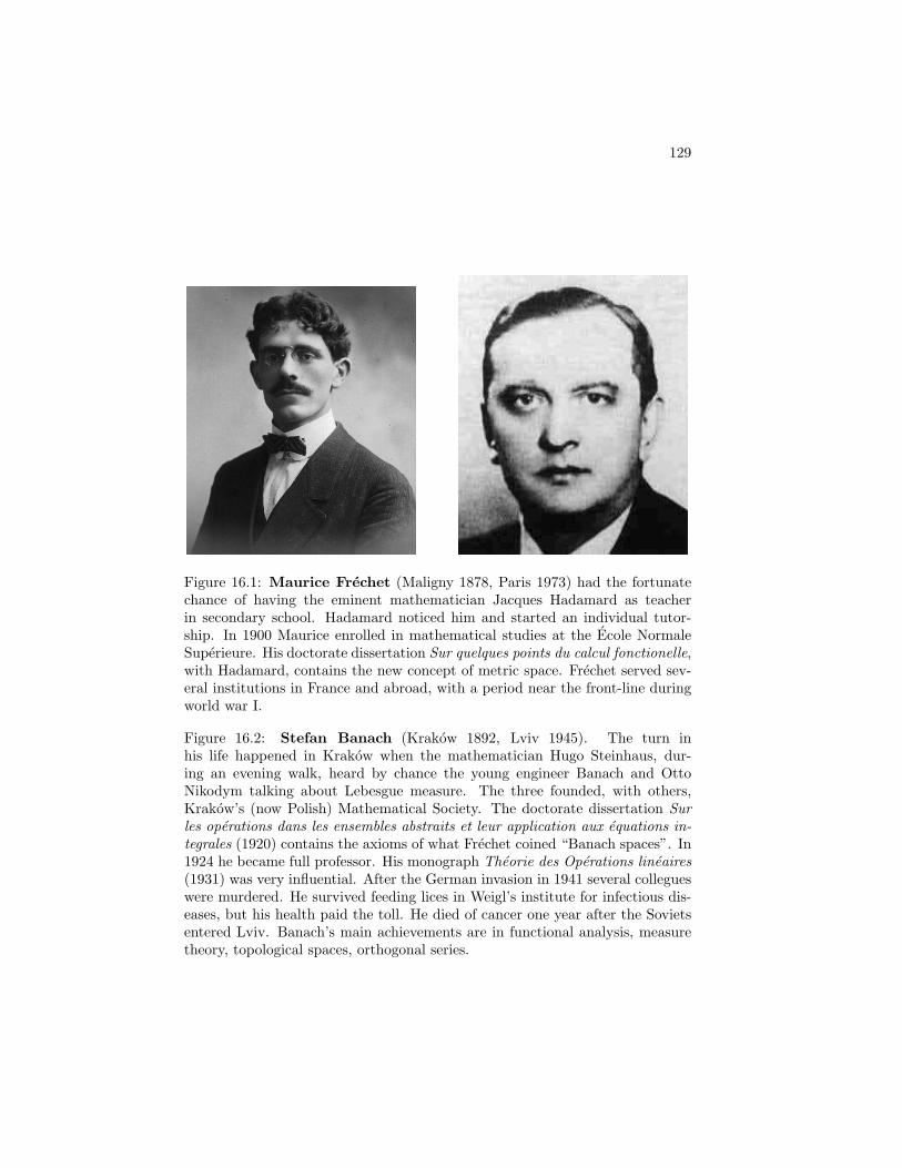
129
Figure 16.1: Maurice Frechet (Maligny 1878, Paris 1973) had the fortunatechance of having the eminent mathematician Jacques Hadamard as teacherin secondary school. Hadamard noticed him and started an individual tutor-ship. In 1900 Maurice enrolled in mathematical studies at the Ecole NormaleSuperieure. His doctorate dissertation Sur quelques points du calcul fonctionelle,with Hadamard, contains the new concept of metric space. Frechet served sev-eral institutions in France and abroad, with a period near the front-line duringworld war I.
Figure 16.2: Stefan Banach (Krakow 1892, Lviv 1945). The turn inhis life happened in Krakow when the mathematician Hugo Steinhaus, dur-ing an evening walk, heard by chance the young engineer Banach and OttoNikodym talking about Lebesgue measure. The three founded, with others,Krakow’s (now Polish) Mathematical Society. The doctorate dissertation Surles operations dans les ensembles abstraits et leur application aux equations in-tegrales (1920) contains the axioms of what Frechet coined “Banach spaces”. In1924 he became full professor. His monograph Theorie des Operations lineaires(1931) was very influential. After the German invasion in 1941 several collegueswere murdered. He survived feeding lices in Weigl’s institute for infectious dis-eases, but his health paid the toll. He died of cancer one year after the Sovietsentered Lviv. Banach’s main achievements are in functional analysis, measuretheory, topological spaces, orthogonal series.
Chapter 17
METRIC SPACES
There are many contexts in mathematics where, given two items x and y (func-tions, sequences, operators, ...), one wishes to quantify how much they differ. In1906 Maurice Frechet, in his doctorate thesis, gave the axioms of a very generalstructure, the Metric Space, that allows to discuss topological concepts thatarise in most situations of analysis.Soon after, in 1914, Felix Hausdorff gave the axioms for Topological Spaces, themost general conceptualization of “nearness”.
17.1 Metric spaces and completeness
Definition 17.1.1. A Metric Space (X, d) is a set X equipped with a dis-tance between pairs of elements. A distance is characterized by the naturalrequirements of being symmetric, non negative, and constrained by the trian-gular inequality:
d(x, y) = d(y, x); (17.1)
d(x, x) = 0, d(x, y) > 0 if x = y; (17.2)
d(x, y) ≤ d(x, z) + d(z, y) ∀x, y, z. (17.3)
The distance defines a topology on X, i.e. a family of neighbourhoods at eachpoint x. Such a family is the set of disks centred in x with radii r > 0:
D(x, r) = y ∈ X : d(x, y) < r.
With this definition, a metric space is a Topological Hausdorff Space. Thefollowing definitions are of great relevance:
Definition 17.1.2. A sequence xn in X is convergent to x ∈ X if the sequenceof distances d(xn, x) converges to zero, i.e.
∀ϵ > 0 ∃Nϵ such that d(xn, x) < ϵ ∀n > Nϵ.
Definition 17.1.3. A sequence xn is a Cauchy sequence (or a fundamentalsequence) if
∀ϵ ∃Nϵ such that d(xm, xn) < ϵ ∀m,n > Nϵ.
130
CHAPTER 17. METRIC SPACES 131
Exercise 17.1.4. Prove that if xn is a Cauchy sequence in a metric space, andxnj is a subsequence with limit x, then xn → x. Hint: use the triangle inequality
d(xn, x) ≤ d(xn, xnj ) + d(xnj , x).
Every convergent sequence is a Cauchy sequence (by the triangle inequality),but a Cauchy sequence may not be convergent. We are thus led to introducethe important definition:
Definition 17.1.5. Ametric space (X, d) is complete if every Cauchy sequenceis convergent in X.
Completeness is a fundamental property: once a metric space is established tobe complete, the Cauchy criterion ensures convergence of a sequence withoutknowledge of the limit.
Theorem 17.1.6. If a metric space X is not complete, it is always possible toconstruct a metric space X, the completion of X, which is complete.
Proof. Consider the set of Cauchy sequences xn in X. Two sequences are equiv-alent, xn ∼ x′n, if they definitely approach:
∀ϵ ∃ Nϵ : d(xn, x′m) < ϵ ∀m,n > Nϵ
The reflexive and symmetric properties are obvious, the transitive property istrue by the triangle inequality: if xn ∼ x′n and x′n ∼ x′′n then: d(xn, x
′′m) ≤
d(x′n, xp) + d(x′′m, xp) ≤ 2ϵ for all m,n, p > max(Nϵ, N′ϵ), i.e. xn ∼ x′′n.
Define X as the set of equivalence classes of Cauchy sequences in X. Suchclasses are of two types: for every x ∈ X there is a class [x] containing theconstant sequence x and equivalent ones; the other type are the classes [xn] ofCauchy sequences with no limit in X.X is a linear space by the rules: [xn + yn] = [xn] + [yn] and λ[xn] = [λxn]. It isa metric space with the distance
d([xn], [yn]) = limn→∞
d(xn, yn)
A finite limit exists because d(xn, yn) is a Cauchy sequence in R: |d(xn, yn) −d(xm, ym)| ≤ |d(xn, yn) − d(xn, ym)| + |d(xm, ym) − d(xn, ym)| ≤ d(yn, ym) +d(xm, xn) < 2ϵ for m,n > Nϵ because xn and yn are Cauchy sequences.X is complete: let [xn]m be a Cauchy sequence (a Cauchy sequence of equivalentCauchy sequences): then d([xn]p, [xn]q) = limn→∞ d(xn,p, xn,q) ≤ ϵ for p, q >Nϵ. The sequence zn = xn,n is a Cauchy sequence: d(zn, zm) = d(xn,n, xm,m) ≤d(xn,n, xn,p) + d(xn,p, xm,p) + d(xm,m, xm,p) < 3ϵ for large enough n,m, p.The class [zn] is the limit in X of the Cauchy sequence: d([xn]m, [zn]) =limn→∞ d(xn,m, xn,n) → 0.
17.2 Maps between metric spaces
Let f : X → Y be a map between metric spaces, with domain D(f). Theimage of the domain is the range Ranf = y ∈ Y : y = f(x), x ∈ D(f).
CHAPTER 17. METRIC SPACES 132
Definition 17.2.1 (Continuity). A map f is continuous at x if:
∀ϵ ∃ δϵ,x such that d(f(x′), f(x))Y < ϵ ∀x′ ∈ D(f) with d(x′, x)X < δϵ,x.
The map f is continuous if it is continuous at all x ∈ D(f).A map f is sequentially continuous if any convergent sequence xn → x in D(f)is mapped to a convergent sequence f(xn) → y in Y .
Theorem 17.2.2. f is continuous if and only if f is sequentially continuous.
Proof. Suppose that f is continuous and xn → x in D(f). Then ∀ϵ > 0 ∃ δϵ,xsuch that d(f(xn), f(x)) < ϵ for all xn such that d(xn, x) < δϵ,x i.e. for alln > Nδ. This means precisely that f(xn) → f(x).To prove the converse, suppose that xn → x and x′n → x (same limit). Thenf(xn) and f(x
′n) converge by hypothesis. The limits coincide (suppose that they
differ, then the sequence x′′2n = xn and x′′2n+1 = x′n converges to x but f(x′′n)has no limit, contrary to the hypothesis). Therefore all sequences that convergeto x are mapped to sequences that converge to y. This implies continuity:limz→x f(z) = y (otherwise a sequence of points zn belonging to disks d(zn, x) <(1/n) for n large enough, would be mapped to a limit different from y).
17.3 Contractive maps
Definition 17.3.1. A map A : X → X is a contraction if there is a constantα < 1 such that d(Ax,Ay) ≤ αd(x, y) for every pair in X.
Exercise 17.3.2. Show that a contraction is a continuous map.
A point x ∈ X is a fixed point for a map A : X → X if Ax = x. Contractionshave this fundamental property:
Theorem 17.3.3 (Fixed point theorem). Every contraction on a completemetric space has a unique fixed point.
Proof. Given an initial point x0, let xk = Akx0 be the sequence generated byiteration of the map. Let’s show that xk is a Cauchy sequence; for n > m:
d(xn, xm) = d(Axn−1, Axm−1) ≤ αd(xn−1, xm−1) ≤ . . . ≤ αmd(xn−m, x0)
≤ αm[d(xn−m, xn−m−1) + . . .+ d(x2, x1) + d(x1, x0)]
≤ αm[αn−m−1 + . . .+ α+ 1] d(x1, x0) ≤ αm
1− αd(x1, x0)
If m is large enough the estimate can be made smaller than any prefixed ϵ.Because of completeness, the Cauchy sequence converges to a limit x. Since Ais continuous: Ax = A limn xn = limnAxn = limn xn+1 = x. Then a fixed pointx exists (and is the limit of the sequence of iterates of a point).Unicity is now proven. Suppose that a different fixed point y exists. The equalityd(x, y) = d(Ax,Ay) ≤ αd(x, y) implies d(x, y) = 0.
Example 17.3.4 (Kepler’s equation). A planet’s orbit is an ellipse with semi-axisa and b and parametric equation x = a cosE, y = b sinE, where the angle E is the
CHAPTER 17. METRIC SPACES 133
eccentric anomaly. The angle varies in time according to Kepler’s equation, whichtranslates the area law:
M = E − e sinE,
e < 1 is the eccentricity and the mean anomaly M = 2πt/T is measured by the time tfrom the perihelion passage, and T is the orbital period.Kepler’s equation is transcendental; it can written as a fixed point problem E = K(E)where the function K(E) = M + e sinE maps [0, 2π] in itself, and is a contraction:
|K(E)−K(E′)| = e| sinE − sinE′| = e| cosE∗| |E − E′| ≤ e|E − E′|
Kepler’s equation may then be solved by iteration. The initial value E = M can be
used, and convergence is faster the smaller is the eccentricity e.
Example 17.3.5 (Volterra’s equation). Consider the integral equation, with realλ and g ∈ C [0, 1], K a continuous function on the unit square:
u(x) = g(x) + λ
∫ x
0
dyK(x, y)u(y), x ∈ [0, 1] (17.4)
It can be written as a fixed point equation in C [0, 1] equipped with the sup norm:Tu = u with (Tu)(x) = g(x) + λ
∫ x
0dyK(x, y)u(y). Let us evaluate:
|(Tu1)(x)− (Tu2)(x)| ≤|λ|∫ x
0
dy|K(x, y)||u1(y)− u2(y)|
≤|λ| supy∈[0,1]
|u1(y)− u2(y)|∫ x
0
dy|K(x, y)|
≤|λ|K ∥u1 − u2∥ K = supx∈[0,1]
∫ x
0
dy|K(x, y)|
Take the sup x ∈ [0, 1]: ∥Tu1 −Tu2∥ ≤ |λ|K ∥u1 − u2∥. If λK < 1, T is a contraction
and the equation u = Tu has a unique solution in C [0, 1], which may be obtained by
iteration: u0 = g, u1 = Tg, u2 = Tu1 . . . .
Chapter 18
BANACH SPACES
18.1 Normed and Banach spaces
Definition 18.1.1. A linear space X equipped with a norm is a normedspace. A norm is defined by the properties (x ∈ X, λ ∈ C):
∥λx∥ = |λ|∥x∥; (18.1)
∥x∥ ≥ 0, ∥x∥ = 0 ⇔ x = 0; (18.2)
∥x1 + x2∥ ≤ ∥x1∥+ ∥x2∥. (18.3)
The definition of abstract normed space was given in the years 1920 - 22by various authors, the most influential being the Polish mathematician StefanBanach. It is straightforward to check that a normed space is a metric spacewith distance
d(x1, x2) = ∥x1 − x2∥ (18.4)
A sequence xn converges to x if ∥xn − x∥ → 0.
Definition 18.1.2. ABanach space is a complete normed space (every Cauchysequence is convergent).
Example 18.1.3. The set C [a, b] of continuous functions f : [a, b] → C is aBanach space with the sup-norm:
∥f∥∞ = supa≤x≤b
|f(x)|
Proof. Completeness: let fn be a Cauchy sequence: ∀ϵ > 0 ∃Nϵ such thatfor all n,m > Nϵ it is supx |fn(x) − fm(x)| < ϵ. This implies that for eachx ∈ [a, b], the sequence fn(x) is a Cauchy sequence in C. Then it convergesto a complex number which we name f(x). This defines a function f . Asm→ ∞, the Cauchy condition becomes supx |fn(x)− f(x)| < ϵ, i.e. fn → f inthe sup-norm. It remains to show that f belongs to C [a, b]. This amounts toprove that a uniformly convergent sequence of continuous functions convergesto a continuous function. Continuity of f is proven as follows: |f(x)− f(y)| ≤|f(x) − fn(x)| + |f(y) − fn(y)| + |fn(x) − fn(y)| ≤ 3ϵ for |x − y| small and nlarge enough.
134
CHAPTER 18. BANACH SPACES 135
The following linear spaces are Banach spaces in the sup norm:C (R) (the set of continuous and bounded complex functions),C∞(R) (the set of continuous functions that vanish at infinity). It is the comple-tion of the normed space C0(R) (the set of continuous functions with compactsupport).
18.2 The Banach spaces Lp(Ω)
Let Ω be Rn or a measurable subset, and consider the set of complex valuedLebesgue measurable functions f : Ω → C. The sum of two functions and theproduct by a complex number λ are defined pointwise: (f +g)(x) = f(x)+g(x)and (λf)(x) = λf(x), and are measurable functions.
18.2.1 L1(Ω) (Lebesque integrable functions)
Consider the measurable functions on Ω such that∫Ω
dx |f(x)| <∞ (18.5)
Since |f(x) + g(x)| ≤ |f(x)| + |g(x)| and |λf(x)| = |λ||f(x)|, it turns out thatf + g and λf are in L 1(Ω) if f and g are. Then L 1(Ω) is a linear space.
The integral (18.5) cannot define a norm because∫|f | dx = 0 implies f = 0
a.e. (almost everywhere) i.e. infinitely many functions, not the single nullelement f = 0 of the linear space. The remedy is to identify these functions byintroducing equivalence classes: two functions f, g ∈ L 1 are equivalent if f = ga.e.Let [f ] be the equivalence class containing f and all functions that differ fromit on a set of measure zero. The set of equivalence classes of functions in L 1(Ω)is a linear space with: [f ] + [g] = [f + g] and λ[f ] = [λf ]. The linear space isL1(Ω), and it is a normed space with the norm1
∥f∥1 =
∫Ω
|f | dx (18.6)
Theorem 18.2.1 (Riesz - Fisher). L1(Ω) is complete (is a Banach space).
Proof. Let fn be a Cauchy sequence in L1: ∀ϵ it is ∥fn − fm∥1 < ϵ forn,m > Nϵ. A sufficient condition for convergence in L1 of a Cauchy sequenceis convergence of a suitable subsequence (the limits coincide).For the choices ϵ = 1/2, 1/22, . . . , 1/2k, . . . the Cauchy condition is satisfied forNϵ = N1, N2, . . . Nk, . . . The subsequence fN1 , . . . , fNk
, . . . has the property∥fNk+1
− fNk∥1 < 2−k. Consider the sequence of functions:
Sm(x) = |fN1(x)|+m∑
k=1
|fNk+1(x)− fNk
(x)|
1) Sm(x) ≥ 0 a.e.2) Sm+1(x) ≥ Sm(x) a.e.
1as f can be any function in [f ], purists avoid writing f(x), which can be any value bychanging f within its class.
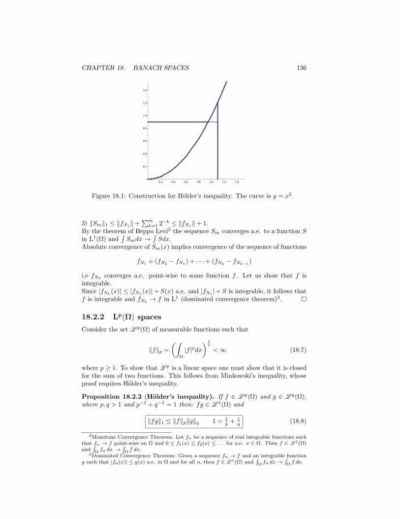
CHAPTER 18. BANACH SPACES 136
0.2 0.4 0.6 0.8 1.0 1.2 1.4
0.2
0.4
0.6
0.8
1.0
1.2
1.4
Figure 18.1: Construction for Holder’s inequality. The curve is y = x2.
3) ∥Sm∥1 ≤ ∥fN1∥+∑m
k=1 2−k ≤ ∥fN1∥+ 1.
By the theorem of Beppo Levi2 the sequence Sm converges a.e. to a function Sin L1(Ω) and
∫Smdx→
∫Sdx.
Absolute convergence of Sm(x) implies convergence of the sequence of functions
fN1 + (fN2 − fN1) + · · ·+ (fNk− fNk−1
)
i.e fNkconverges a.e. point-wise to some function f . Let us show that f is
integrable.Since |fNk
(x)| ≤ |fN1(x)|+ S(x) a.e. and |fN1 |+ S is integrable, it follows thatf is integrable and fNk
→ f in L1 (dominated convergence theorem)3.
18.2.2 Lp(Ω) spaces
Consider the set L p(Ω) of measurable functions such that
∥f∥p =
(∫Ω
|f |pdx) 1
p
<∞ (18.7)
where p ≥ 1. To show that L p is a linear space one must show that it is closedfor the sum of two functions. This follows from Minkowski’s inequality, whoseproof requires Holder’s inequality.
Proposition 18.2.2 (Holder’s inequality). If f ∈ L p(Ω) and g ∈ L q(Ω),where p, q > 1 and p−1 + q−1 = 1 then: fg ∈ L 1(Ω) and
∥fg∥1 ≤ ∥f∥p∥g∥q 1 = 1p + 1
q (18.8)
2Monotone Convergence Theorem: Let fn be a sequence of real integrable functions suchthat fn → f point-wise on Ω and 0 ≤ f1(x) ≤ f2(x) ≤ . . . for a.e. x ∈ Ω. Then f ∈ L 1(Ω)and
∫Ω fn dx →
∫Ω f dx.
3Dominated Convergence Theorem: Given a sequence fn → f and an integrable functiong such that |fn(x)| ≤ g(x) a.e. in Ω and for all n, then f ∈ L 1(Ω) and
∫Ω fn dx →
∫Ω f dx.
CHAPTER 18. BANACH SPACES 137
Proof. Consider the curve y = xp−1 in the positive xy quadrant. Inversion givesx = yq−1. Fix on the x and y axis two arbitrary positive numbers u and v. Thearea of the rectangle uv is not greater than the sum of two areas: the areabounded by the curve in the strip 0 ≤ x ≤ u, and the area bounded by thecurve in the strip 0 ≤ y ≤ v:
uv ≤∫ u
0
dx xp−1 +
∫ v
0
dy yq−1 =up
p+vq
q.
Put u = |f(x)|/∥f∥p and v = |g(x)|/∥g∥q and integrate in x on Ω; the inequalityis obtained.
Remark 18.2.3. If m(Ω) <∞, one may take g = 1 in Holder’s inequality, andnote that if f ∈ L p(Ω) then f ∈ L 1(Ω), i.e. L p(Ω) ⊆ L 1(Ω), for any p > 1.
Proposition 18.2.4 (Minkowski’s inequality). If f , g in L p(Ω) then:
∥f + g∥p ≤ ∥f∥p + ∥g∥p (18.9)
Proof. For u, v, z > 0, 1p + 1
q = 1, consider the Holder inequalities:
uzp−1 ≤ up
p+zp
q, vzp−1 ≤ vp
p+zp
q
Put u = |f(x)|/∥f∥p, v = |g(x)|/∥g∥p, z = |f(x)+g(x)|/∥f +g∥p and integrate:∫Ω
dx|f(x)|∥f∥p
|f(x) + g(x)|p−1
∥f + g∥p−1p
≤ 1,
∫Ω
dx|g(x)|∥g∥p
|f(x) + g(x)|p−1
∥f + g∥p−1p
≤ 1
The two inequalities give:∫Ω
dx(|f(x)|+ |g(x)|) |f(x) + g(x)|p−1 ≤ (∥f∥p + ∥g∥p)∥f + g∥p−1p
Since |f(x) + g(x)| ≤ |f(x)|+ |g(x)|, the inequality becomes:∫Ω
dx|f(x) + g(x)|p ≤ (∥f∥p + ∥g∥p)∥f + g∥p−1p
i.e. ∥f + g∥pp ≤ (∥f∥p + ∥g∥p)∥f + g∥p−1p , and the identity follows.
The inequality implies that L p(Ω) is a linear space. To promote ∥f∥p to anorm one must switch to the set of equivalence classes. Minkowski’s inequalityproves the triangle inequality, and Lp(Ω) is a normed space. The Riesz-Fishertheorem states that it is complete (a Banach space) for all p ≥ 1.
Holder’ inequality shows that the functions of Lq(Ω) define linear continuousfunctionals on Lp(Ω) if 1/p + 1/q = 1. One actually proves that a space is thedual of the other. The dual of L1(Ω) is the space L∞(Ω) (but the dual of L∞
contains L1, see Reed and Simon, Functional Analysis, Academic Press).
18.2.3 L∞(Ω) space
L ∞(Ω) is the space of measurable functions f : Ω → C that are a.e. bounded:given f , there is a constant Mf such that the set where |f(x)| > Mf hasLebesgue measure zero. The inf of such bounds Mf is ∥f∥∞, which becomesa norm for the equivalence classes of functions that are equal a.e. The spaceL∞(Ω) is a Banach space.C (R) is a subspace of L ∞(R). The norm coincides with the sup-norm.
CHAPTER 18. BANACH SPACES 138
18.3 Continuous and bounded maps
Hereafter A : X → Y is a map (the term “operator” will be used) betweennormed spaces, with domain D(A). The image of the domain is the rangeRanA = y ∈ Y : y = Ax, x ∈ D(A), the kernel is the set KerA = x ∈ X :Ax = 0. We recall a definition and a result exported from the more generalcontext of metric spaces:
Definition 18.3.1. A map A is continuous at x in D(A) if:
∀ϵ ∃ δϵ,x such that ∥Ax′ − Ax∥Y < ϵ ∀x′ ∈ D(A) with ∥x′ − x∥X < δϵ,x.
The map is continuous if it is continuous at all x ∈ D(A). It is sequentiallycontinuous if any convergent sequence in D(A) is mapped to a convergent se-quence.
Theorem 18.3.2. A is continuous if and only if A is sequentially continuous.
Remark 18.3.3. The kernel of a continuous operator is a closed set. (Supposethat xn is a sequence in KerA and xn → x ∈ D(A). Then Ax = limY Axn = 0i.e. x ∈ KerA).
Definition 18.3.4. A is bounded if there is a constant CA > 0 such that∥Ax∥Y < CA∥x∥X for all x ∈ D(A).
Definition 18.3.5. A is linear if D(A) is a linear subspace and A(x+ λx′) =Ax+ λAx′ for all x, x′ ∈ D(A), λ ∈ C.
Remark 18.3.6. If A is linear, then A is continuous if and only if it is con-tinuous at x = 0.
Theorem 18.3.7. A linear map A : D(A) → Y is bounded if and only if it iscontinuous.
Proof. Suppose that A is bounded and xn → 0 in D(A). Then ∥Axn∥ ≤CA∥xn∥ → 0 i.e. A is sequentially continuous in the origin i.e. A is continuous.Let A be continuous. Then for ϵ = 1 there is δ > 0 such that ∥Ax∥ < 1 forall x in the domain with ∥x∥ < δ. For any y ∈ D(A), put x = yδ/∥y∥ then∥Ay∥ = ∥y∥∥Ax∥δ−1 ≤ δ−1∥y∥ i.e. A is bounded.
Theorem 18.3.8. Let X be a normed space and Y a Banach space. A linearbounded operator A : D(A) ⊂ X → Y extends uniquely to a linear bounded
operator on the closure of the domain: A : D(A) → Y .
Proof. If x ∈ D there is a convergent sequence xn in D with limit x. A conver-gent sequence is Cauchy, therefore ∥Axn − Axm∥Y ≤ CA∥xn − xm∥X ≤ ϵ forn,m > Nϵ i.e. Axn is Cauchy in Y . Since Y is Banach, Axn → y.Define Ax = y. The domain D(A) is a linear space: if xn → x and x′n → x′
in D(A), then xn + x′n → x + x′ and λxn → λx. A is linear: A(x + x′) =limn Axn + limn Ax
′n = Ax+Ax′. A is bounded: since the norm is continuous,
∥Ax∥ = limn ∥Axn∥ ≤ CA limn ∥xn∥ = CA∥x∥.
CHAPTER 18. BANACH SPACES 139
18.3.1 The inverse operator
If A : X → Y is an operator with domain D(A), the inverse operator A−1 :Y → X exists if A is injective, i.e. Ax = Ax′ implies x = x′. Then, if Ax = yit is A−1y = x, with D(A−1) = Ran A, and Ran A−1 = D(A).
Proposition 18.3.9. If A is linear, A−1 exists if and only if Ker A = 0. IfA−1 exists, it is linear.
Proof. The condition Ax = Ay if and only if x = y is equivalent to A(x−y) = 0iff x− y = 0 i.e. Ker (A) = 0.If Ax = y and Ax′ = y′ then A(λx + x′) = λy + y′. The inverse is such thatx = A−1y, x′ = A−1y′ and λx + x′ = A−1(λy + y′), i.e. λA−1y + A−1y′ =A−1(λy + y′), i.e. A−1 is linear.
18.4 Linear bounded operators on X
The set L (X,Y ) of linear operators on a normed space X, with domain X, toa normed space Y , is a linear space with the definitions
(A+ B)x = Ax+ Bx, (λA)x = λ(Ax), x ∈ X, λ ∈ C.
If two operators are bounded, their linear combinations are bounded. B(X,Y )is the linear space of linear and bounded operators from X to Y .The existence of a bound is a very useful property of an operator A. The bestbound is the least constant CA such that ∥Ax∥Y /∥x∥X ≤ CA for all x ∈ X,x = 0. This constant is the operator norm of A:
∥A∥ = supx∈X,x =0
∥Ax∥Y∥x∥X
= sup∥x∥X=1
∥Ax∥Y (18.10)
As a consequence the best inequality is
∥Ax∥Y ≤ ∥A∥∥x∥X , ∀x ∈ X.
Eq.(18.10) defines a norm and makes B(X,Y ) a normed space: if ∥A∥ = 0 it is∥Ax∥Y = 0 for all x, i.e. A = 0. The property ∥λA∥ = |λ|∥A∥ is straightforward.The triangle inequality: ∥A+B∥ = sup∥x∥=1 ∥(A+B)x∥Y ≤ sup∥x∥=1(∥Ax∥Y +
∥Bx∥Y ) ≤ sup∥x∥=1 ∥Ax∥Y + sup∥x∥=1 ∥Bx∥Y = ∥A∥+ ∥B∥.
Theorem 18.4.1. If Y is a Banach space, then B(X,Y ) is a Banach space.
Proof. Let An be a Cauchy sequence of operators in B(X,Y ):
∀ϵ ∃Nϵ s.t. ∥An −Am∥ < ϵ ∀n,m ≥ Nϵ
1) ∥An∥ is a Cauchy sequence in R, by the inequality4∣∣∣ ∥An∥ − ∥Am∥
∣∣∣ ≤ ∥An−Am∥. Then ∥An∥ → C ≥ 0.2) Anx is a Cauchy sequence in Y by the inequality
∥Anx− Amx∥Y ≤ ∥An − Am∥∥x∥X4By the triangular property of a norm, ∥x∥ ≤ ∥x−y∥+∥y∥, it is always ∥x∥−∥y∥ ≤ ∥x−y∥.
The same holds with x and y exchanged, so the modulus can be taken.
CHAPTER 18. BANACH SPACES 140
Since Y is complete, Anx converges. Define A as the operator Ax = limn Anx.A is a linear operator: A(x+λy) = limn An(x+λy) = limn Anx+λ limn Any =Ax+ λAy.3) The inequality in 2) implies: ∥Anx− Amx∥Y ≤ (∥An∥+ ∥Am∥)∥x∥X . for allm,n > Nϵ. In particular, for unfinite m: ∥Anx − Ax∥Y ≤ (∥An∥ + C)∥x∥X .Therefore An − A is bounded, i.e. A is bounded.Is A the limit of An in the B(X,Y ) topology? ∥An − A∥ = sup∥x∥=1 ∥Anx −Ax∥Y . The norm is continuous and Anx− Ax→ 0, then ∥An − A∥ → 0.
Remark 18.4.2. Convergence An → A in B(X,Y ) implies Anx → Ax in Y ,for any x (norm convergence implies strong convergence).
18.4.1 The dual space
In 1929 Banach introduced the important notion of dual space X∗ of a Ba-nach space X: it is the space of bounded linear functionals B(X,C). Since Cis complete, X∗ is a Banach space.
There are two ways by which a sequence may converge in X:1) xn → x strongly if ∥xn − x∥X → 0;2) xn → x weakly if Fxn → Fx in C for all F ∈ X∗.
There are three ways by which a sequence of operators in B(X,Y ) converges:1) An converges in norm to A if ∥An − A∥ → 0;2) An converges strongly if Anx converges in Y -norm for all x ∈ X;3) An converges weakly if FAnx converges in C for all x ∈ X, F ∈ Y ∗.
18.5 The Banach algebra B(X)
If X = Y , the space B(X) ≡ B(X,X) is closed for the product. If A andB are linear and bounded operators X → X, the operator AB is defined by(AB)x = A(Bx). The product is linear and bounded: ∥(AB)x∥ ≤ ∥A∥ ∥Bx∥ ≤(∥A∥∥B∥)∥x∥. Therefore:
∥AB∥ ≤ ∥A∥ ∥B∥ (18.11)
Then B(X) is an associative algebra (associative and distributive properties)with unit (the identity operator).
18.5.1 The inverse of a linear operator
Suppose that A ∈ B(X) is invertible, and that Ran A = X, so that D(A−1) =X. The inverse operator need not be bounded. From ∥x∥X = ∥AA−1x∥X ≤∥A∥∥A−1x∥X for all x, it is
∥A−1x∥∥x∥
≥ 1
∥A∥(18.12)
If A−1 is bounded, then ∥A−1∥ ≥ ∥A∥−1.
CHAPTER 18. BANACH SPACES 141
Theorem 18.5.1 (Neumann). If X is a Banach space, A ∈ B(X), and∥A∥ < 1, then (1− A)−1 exists in B(X) and is given by the Neumann series:
(1− A)−1 =
∞∑k=0
Ak (18.13)
Proof. Consider the partial sums Sn = I + A+ A2 + · · ·+ An in B(X). It is aCauchy sequence in the operator norm ∥Sn+m− Sm∥ = ∥Am+1+ · · ·+ Am+n∥ ≤∥A∥m+1+ · · ·+∥A∥m+n ≤ ∥A∥m+1
1−∥A∥ < ϵ for m > N , all n. Therefore the sequence
of partial sums converges to the geometric series∑
k Ak in B(X).
Since (1− A)Sn = 1− An+1 → 1 in the limit n→ ∞, (18.13) is proven.
18.5.2 Power series of operators
The Neumann series is the operator analogous to the geometric series in complexanalysis. Several important complex functions that are expressed as power seriesmay be extended to functions of operators. For A ∈ B(X), consider the operatorand the complex power series
f(A) =
∞∑n=0
cnAn, f(z) =
∞∑n=0
cnzn
If SN are the operator partial sums, it is ∥SN+p − SN∥ = ∥∑N+p
n=N+1 cnAn∥ ≤∑N+p
n=N+1 |cn| ∥A∥n. Therefore, the partial sums form a Cauchy sequence in
B(X) if the partial sums of the power series f(∥A∥) are a Cauchy sequence inC. A sufficient condition is that ∥A∥ < R where R is the radius of convergenceof the power series f(∥A∥).Exercise 18.5.2. Show that if A and f(A) are in B(X), and if Ax = λx,where x ∈ X, then F (A)x = f(λ)x.
Example 18.5.3 (The exponential of an operator).If A ∈ B(X) and z ∈ C, then the exponential series
ezA =∞∑k=0
(zA)k
k!(18.14)
always converges in the operator norm to a bounded operator and
ezAewA = e(z+w)A (18.15)
This is proven by evaluating the Cauchy product of the partial sums EN :
EN (z)EN (w) =
2N∑k=0
Akk∑
m=0
zmwk−m
m!(k −m)!=
2N∑k=0
Ak (z + w)k
k!= E2N (z + w)
Since the limits N → ∞ exist for the single partial sums, the result follows.Let us show that
d
dzezA ≡ lim
h→0
1
h[e(z+h)A − eA] = A ezA
Proof: ∥ 1h [e
(z+h)A − ezA]− AezA∥ ≤ ∥ezA∥ ∥ ehA−1h − A∥. The last norm is zero
for h→ 0.
CHAPTER 18. BANACH SPACES 142
Remark 18.5.4. The property (18.15) extends to commuting operators:
eAeB = eA+B if and only if AB = BA
For non-commuting operators, the right hand side is evaluated by the Baker -Campbell - Hausdorff formula.
Chapter 19
HILBERT SPACES
The theory of Hilbert spaces originates in the studies of David Hilbert and hisstudent Erhard Schmidt on integral equations. They have a long hystory, whosebeginning might be the introduction of the Laplace transform to solve lineardifferential equations1 (1782). The classification of linear integral equationsbears the names of Vito Volterra (1860-1940) and Ivar Fredholm (1866-1927),who gave a substantial contribution.The relevance of Hilbert spaces for the mathematical foundation of quantummechanics led John von Neumann to give them an axiomatic setting, in theyears 1929-30.
19.1 Inner product spaces
Definition 19.1.1 (Inner product). A linear space H (on C) is an InnerProduct Space (or pre-Hilbert space) if there is a map (the inner product)( | ) : H × H → C such that for all x, y, z ∈ H and λ ∈ C:
(x|x) ≥ 0 and (x|x) = 0 iff x = 0 (19.1)
(x|y + z) = (x|y) + (x|z) (19.2)
(x|λy) = λ(x|y) (19.3)
(x|y) = (y|x). (19.4)
The properties imply antilinearity in the first argument2:
(x+ λy|z) = (x|z) + λ(y|z).
For real spaces the rule (19.4) is replaced by (x|y) = (y|x), which implies bi-linearity (linearity in both arguments of the inner product).It will be shown that the inner product induces a norm; we begin by introducingthe notation ∥x∥ =
√(x|x).
Exercise 19.1.2. Show that: 1) (x|0) = 0; 2) if (x|y) = 0 ∀y then x = 0.
1Bateman, Report on the hystory and present state of the theory of integral equations,http://www.biodiversitylibrary.org/item/94115#page/507/mode/1up
2In the mathematical literature the inner product is often defined to be linear in the firstand antilinear in the second argument. Physicists prefer the converse.
143
CHAPTER 19. HILBERT SPACES 144
Definition 19.1.3. Two vectors x and x′ are orthogonal, x ⊥ x′, if (x|x′) = 0.A set of vectors u1, . . . , un is an orthonormal set if (ui|uj) = δij .
Pythagoras’ relation holds: if x ⊥ x′ then ∥x+ x′∥2 = ∥x∥2 + ∥x′∥2.
Theorem 19.1.4 (Bessel’s inequality). Let uknk=1 be an orthonormal set,then for any x:
∥x∥2 ≥n∑
k=1
|(uk|x)|2 (19.5)
Proof. Set x′ =∑
k(uk|x)uk; since it is the sum of orthonormal vectors, ∥x′∥2 =∑k |(uk|x)|2. Next, let’s show that x′ and x− x′ are orthogonal: (x′|x− x′) =
(x′|x)− ∥x′∥2 =∑
k (uk|x)(uk|x)− ∥x′∥2 = 0. Then ∥x∥2 = ∥(x− x′) + x′∥2 =∥x− x′∥2 + ∥x′∥2 ≥ ∥x′∥2.
Bessel’s inequality for n = 1 is a famous and fundamental inequality. It isinstructive to give a direct proof:
Proposition 19.1.5 (Schwarz’s inequality). For all x and y in an innerproduct space H :
|(x|y)| ≤ ∥x∥∥y∥ (19.6)
Proof. For any λ ∈ C, x, y = 0 the full expansion of (x+ λy|x+ λy) ≥ 0 gives:(λ1 +
Re(x|y)∥y∥2
)2
+
(λ2 −
Im(x|y)∥y∥2
)2
+∥x∥2∥y∥2 − |(x|y)|2
∥y∥4≥ 0
Since λ1,2 can be chosen to make the squares vanish, the inequality follows.
Exercise 19.1.6. Show that if ∥x∥ = ∥y∥ = 1 and (x|y) = 1 then x = y. Whatabout two normalised vectors such that |(x|y)| = 1?
Exercise 19.1.7. Show that |(x|y)| = ∥x∥ ∥y∥ if and only if y = λx, λ ∈ C.
19.2 The Hilbert norm
Proposition 19.2.1. An inner product space is a normed space, with norm
∥x∥ =√
(x|x) (19.7)
Proof. We must prove the triangle inequality: ∥x + y∥2 = (x + y|x + y) =(x|x) + 2Re(x|y) + (y|y) ≤ ∥x∥2 + 2|(x|y)| + ∥y∥2 ≤ ∥x∥2 + 2∥x∥∥y∥ + ∥y∥2= (∥x∥+ ∥y∥)2.
The existence of a norm implies notions such as continuity, convergent se-quences, Cauchy property, etc.
Proposition 19.2.2. Fix x ∈ H , the function (x| · ) : H → C is continuous.
Proof. Let yn be a convergent sequence, yn → y; we show that (x|yn) → (x|y):|(x|yn)− (x|y)| = |(x|yn − y)| ≤ ∥x∥∥yn − y∥ → 0.
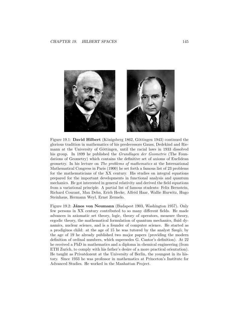
CHAPTER 19. HILBERT SPACES 145
Figure 19.1: David Hilbert (Konigsberg 1862, Gottingen 1943) continued theglorious tradition in mathematics of his predecessors Gauss, Dedekind and Rie-mann at the University of Gottingen, until the racial laws in 1933 dissolvedhis group. In 1899 he published the Grundlagen der Geometrie (The Foun-dations of Geometry) which contains the definitive set of axioms of Euclideangeometry. In his lecture on The problems of mathematics at the InternationalMathematical Congress in Paris (1900) he set forth a famous list of 23 problemsfor the mathematicians of the XX century. His studies on integral equationsprepared for the important developments in functional analysis and quantummechanics. He got interested in general relativity and derived the field equationsfrom a variational principle. A partial list of famous students: Felix Bernstein,Richard Courant, Max Dehn, Erich Hecke, Alfred Haar, Wallie Hurwitz, HugoSteinhaus, Hermann Weyl, Ernst Zermelo.
Figure 19.2: Janos von Neumann (Budapest 1903, Washington 1957). Onlyfew persons in XX century contributed to so many different fields. He madeadvances in axiomatic set theory, logic, theory of operators, measure theory,ergodic theory, the mathematical formulation of quantum mechanics, fluid dy-namics, nuclear science, and is a founder of computer science. He started asa prodigiuos child: at the age of 15 he was tutored by the analyst Szego; bythe age of 19 he already published two major papers (providing the moderndefinition of ordinal numbers, which supersedes G. Cantor’s definition). At 22he received a PhD in mathematics and a diploma in chemical engineering (fromETH Zurich, to comply with his father’s desire of a more practical orientation).He taught as Privatdozent at the University of Berlin, the youngest in its his-tory. Since 1933 he was professor in mathematics at Princeton’s Institute forAdvanced Studies. He worked in the Manhattan Project.
CHAPTER 19. HILBERT SPACES 146
Note the following identities, that express the inner product in terms of theHilbert norm:
Re(x|y) = 14 (∥x+ y∥2 − ∥x− y∥2) (19.8)
Im(x|y) = −14 (∥x+ iy∥2 − ∥x− iy∥2) (19.9)
The Hilbert norm has the parallelogram property, which can be directlychecked out of its definition:
∥x+ y∥2 + ∥x− y∥2 = 2∥x∥2 + 2∥y∥2 (19.10)
Proposition 19.2.3 (Polarization formula). A norm is a Hilbert norm (i.e.there is a inner product such that the norm descends from it) if and only if thenorm fulfils the parallelogram condition.
Proof. We only need proving that a norm with the parallelogram property fol-lows from an inner product. The formulae (19.8) and (19.9) suggest the followingexpression as a candidate for the inner product (for a real space the last twoterms are absent):
(x|y) = 14∥x+ y∥2 − 1
4∥x− y∥2 − i4∥x+ iy∥2 + i
4∥x− iy∥2 (19.11)
The difficult task is to prove linearity in the second argument, the other prop-erties being easy to prove. By repeated use of the parallelogram property,
Re (x|y + z) = 14∥x+ y + z∥2 − 1
4∥x− y − z∥2
= ( 12∥x+ y∥2 + 12∥z∥
2 − 14∥x+ y − z∥2)− 1
4∥x− y − z∥2
= 12∥x+ y∥2 + 1
2∥z∥2 − 1
2∥x− z∥2 − 12∥y∥
2
Now sum to it the expression with y and z exchanged, divide by 2 and obtain
Re (x|y + z) = 14∥x+ y∥2 − 1
4∥x− z∥2 + 14∥x+ z∥2 − 1
4∥x− y∥2
= Re (x|y) + Re (x|z).
The same procedure works for the imaginary part: Im (x|y + z) = Im (x|y) +Im (x|z). Hence the additive property is proven.Linearity for scalar multiplication: for p ∈ N, additivity implies (x|py) = p(x|y).For q ∈ N: p(x|y) = p(x|q(y/q) ) = pq(x|y/q) = q(x|p(y/q)) ⇒ p
q (x|y) =
(x|pq y). Since the inner product is continuous and (x| − y) = −(x|y) (see
(19.11)), the property extends from rationals p/q to real numbers. Moreover,since (x|iy) = i(x|y) holds (see (19.11)), the property holds for complex num-bers.
Exercise 19.2.4. In a normed space, a vector x is orthogonal to y in the senseof Birkhoff-James if and only if ∥x∥ ≤ ∥x+ λy∥ for all λ ∈ C. Prove that in ainner-product space the definition coincides with (x|y) = 0.
Definition 19.2.5. AHilbert space is a inner product space which is completein the Hilbert norm topology.
Example 19.2.6. The linear space Cn is a Hilbert space with the scalar product(z|w) =
∑k zkwk.
CHAPTER 19. HILBERT SPACES 147
Exercise 19.2.7. Show that the set of complex matrices Cn×n is a Hilbert spacewith inner product (A|B) = tr(A†B). The corresponding norm
∥A∥ =√trA†A =
√∑ij
|Aij |2
is known as the Frobenius norm.Show that also (A|B) = tr(M†MA†B) is an inner product, if M is invertible.
Example 19.2.8. L2(Ω) is the Banach space of (equivalence classes of) Lebesguesquare integrable functions, with squared norm ∥f∥22 =
∫Ω|f |2dx. The norm has
the parallelogram property, and descends from the inner product
(f |g) =∫Ω
fg dx (19.12)
This is perhaps the most important space in functional analysis. Depending onthe measurable set Ω, one introduces important families of orthogonal functions(see section 19.4.1).
Exercise 19.2.9. Evaluate the norms of f(x) = 1/(1 + ix) as an element inL1(0, 1) and in L2(0, 1)
Example 19.2.10. The set C [−1, 1] of continuous complex-valued functions on
[−1, 1] is an inner product space with (f |g) =∫ 1
−1dxf(x)g(x), but it is not a
Hilbert space as this counter-example shows:
fn(x) =
−1 −1 ≤ x ≤ −1/n
nx −1/n < x < 1/n
1 1/n ≤ x ≤ 1
(19.13)
is a Cauchy sequence (i.e. ∀ϵ there is N such that∫ 1
−1dx|fn(x)− fm(x)|2 < ϵ2
for all n,m > N) but the limit function (the step function) is not continuous.
19.3 Isomorphism
Definition 19.3.1. Two Hilbert spaces H1 and H2 are isomorphic if there isa linear operator U : H1 → H2 that is a bijection among the two spaces, andconserves the norm ∥Ux∥2 = ∥x∥1 ∀x. U is a unitary operator.
Remark. By the polarization formula (19.11), norm conservation and linearityimply the conservation of inner products: (Ux|Uy)2 = (x|y)1 ∀x, y ∈ H1.
Any complex n-dimensional Hilbert space Hn is isomorphic to Cn. Givenan orthonormal basis uknk=1 an element has expansion x =
∑nk=1 xkuk, with
coefficients xk = (uk|x) that define a vector x ∈ Cn. The map Ux = x is aunitary operator from Hn to Cn.Is there a canonical isomorphism for infinite-dimensional Hilbert spaces? Theanswer is affirmative, with a natural restriction. Let us first introduce theinfinite dimensional analogue of Cn (or Rn for real Hilbert spaces).
CHAPTER 19. HILBERT SPACES 148
19.3.1 Square summable sequences
In 1906 David Hilbert introduced the set ℓ2(C) of complex sequences ak∞k=1
such that∞∑k=1
|ak|2 <∞
It is a linear space: if a = ak and b = bk belong to ℓ2, define a+b = ak+bkand λa = λak. To show that a+b is in ℓ2 note that |ak+bk|2 ≤ |ak|2+ |bk|2+2|akbk| ≤ 2|ak|2 + 2|bk|2 (use 0 < (x− y)2 = x2 + y2 − 2xy).ℓ2(C) is an inner product space with
(a|b) =∞∑k=1
akbk (19.14)
Existence of the inner product follows from 2|akbk| ≤ |ak|2+ |bk|2; formal prop-erties are easily checked.ℓ2(C) has a countable orthonormal basis: e1 = 1, 0, 0, . . . , e2 = 0, 1, 0, . . . ,etc.
Theorem 19.3.2. ℓ2(C) is complete (it is a Hilbert space).
Proof. Let aν be a Cauchy sequence of elements in ℓ2 (a sequence of sequencesaνk), i.e. for any ϵ > 0 there is N such that for all ν, µ > N it is
∥aν − aµ∥2 =
∞∑k=1
|aνk − aµk|2 < ϵ2 (19.15)
We must show that there is a limit sequence a in ℓ2. The above condition impliesthat |aνk − aµk| < ϵ for all k and ν, µ > N , then each sequence aν1, aν2,... is Cauchy and then convergent in C to limits a1, a2 ... Let a = ak be thesequence of such limits.Since (19.15) holds for all ν, µ > Nϵ, let µ = ∞: it is
∑k |aνk − ak|2 < ϵ2,
i.e. the element aν − a belongs to ℓ2. Since aν ∈ ℓ2 it follows by linearity thata ∈ ℓ2. Moreover, ∥aν − a∥ ≤ ϵ, then an → a ∈ ℓ2 in the ℓ2 topology.
Definition 19.3.3. A Hilbert space is separable if it has a countable densesubset.
Theorem 19.3.4. ℓ2(C) is separable.
Proof. Consider the set ℓ′ of sequences q = qk, where qk are complex rationalnumbers (i.e. Re qk, Im qk ∈ Q) for k ≤ n, and 0 for k > n (where eachsequence has its own n). The set ℓ′ is countable and is a subset of ℓ2. We showthat it is dense in ℓ2, i.e. for any element a = ak and any ϵ > 0 there is anelement q of ℓ′ such that ∥a− q∥ < ϵ.Choose n such that
∑∞k=n+1 |ak|2 <
12ϵ
2 and choose q = q1, . . . , qn, 0, 0, . . . such that |ak−qk|2 ≤ ϵ2/2n for all k ≤ n (this is possible since complex rationalnumbers are dense in C). Then: ∥a − q∥2 =
∑nk=1 |ak − qk|2 +
∑k>n |ak|2 <
n ϵ2
2n + 12ϵ
2 = ϵ2.
CHAPTER 19. HILBERT SPACES 149
Example 19.3.5 (A non-separable Hilbert space3). Consider the set E =eωω∈R of functions eω(t) = exp(iωt), t ∈ R. The finite linear combinationsf =
∑ω fωeω with complex numbers fω form a linear space. The following
“time average” is always well defined, and is an inner product:
(f |g) = limT→∞
1
T
∫ T/2
−T/2
f(t)g(t)dt (19.16)
The completion of the linear space with respect to the norm is a Hilbert space.As (eω|eω′) = δω,ω′ , it is ∥eω − eω′∥2 = 2 if ω = ω′. Since E is uncountable,with elements separated by a finite distance, there cannot exist a countable setof functions such that any eω is approximated by a linear combination of suchfunctions (we’d need an uncountable set of approximating functions!). Then theHilbert space is non-separable.
19.4 Orthogonal systems
Given n linearly independent points x1, . . . , xn it is always possible to producelinear combinations u1, . . . , un that form an orthonormal set. The (Gram -Schmidt) orthonormalization procedure is:
y1 = x1, ⇒ u1 = y1/∥y1∥,y2 = x2 − (u1|x2)u1, ⇒ u2 = y2/∥y2∥,y3 = x3 − (u1|x3)u1 − (u2|x3)u2, ⇒ u3 = y3/∥y3∥,. . . . . .
Exercise 19.4.1. Given vectors x1, . . . , xn, introduce the Gram’s matrix Gij =(xi|xj) ∈ Cn×n. Show that:1) the vectors are linearly dependent iff detG = 0;2) the matrix is non-negative (G ≥ 0) i.e. u†Gu ≥ 0 ∀u ∈ Cn;3) detG ≤ ∥x1∥2 · · · ∥xn∥2 (use Hadamard’s inequality for positive matrices).
Exercise 19.4.2. In Cn, given n linearly independent vectors x1, . . . , xn, avector has expansion u =
∑ni=1 cixi. The coefficients ci solve the linear sys-
tem (xi|u) =∑
j Gijcj where G is Gram’s matrix. Obtain the useful formula(Kramer):
u =(−1)
detGdet
0 x1 · · · xn
(x1|u) (x1|x1) · · · (x1|xn)...
......
(xn|u) (xn|x1) · · · (xn|xn)
(19.17)
19.4.1 Orthogonal polynomials
Let p0, p1, . . . be a sequence of real polynomials of degree 0, 1, . . . , that satisfythe orthogonality condition∫
σ
dxω(x) pi(x)pj(x) = hjδij (19.18)
3N.I.Akhiezer and I.M.Glazman, ”Theory of linear operators in Hilbert spaces”, vol 1,par.13 (1961) (Dover reprint).
CHAPTER 19. HILBERT SPACES 150
where ω(x) ≥ 0 is a weight function, σ is a real (possibly unbounded) intervaland hj > 0 are constants.
The table lists some important sets of orthogonal polynomials, that may beobtained by orthogonalization of the monomials 1, x, x2, . . . :
σ ω(x) pkR e−x2
Hk Hermite[0,∞) e−x Lk Laguerre[−1, 1] 1 Pk Legendre
[−1, 1] (1− x2)−12 Tk Chebyshev
[−1, 1] (1− x2)α−12 Cα
k Gegenbauer
Proposition 19.4.3. Orthogonal polynomials satisfy a three-term recurrencerelation with real constants ak, bk and ck:
xpk(x) = akpk+1(x) + bkpk(x) + ckpk−1(x) (19.19)
Proof. Suppose that the recurrence contains also the term dkpk−2(x). Multiply(19.19) by ω(x)pk−2(x) and integrate. All terms but two vanish by orthogonal-ity: ∫
σ
dxω(x)xpk(x)pk−2(x) = dkhk−2.
Since xpk−2 = ak−2pk−1 + . . . , also the left integral vanishes by orthogonality.Therefore dk = 0. In the same way one proves the absence of all lower orderterms in the recurrence.
The constants ak may be chosen positive. The recurrence relation can be writtenin multiplicative form:[
pk+1(x)pk(x)
]=
[(x− bk)/ak −ck/ak
1 0
] [pk(x)pk−1(x)
]Iteration provides the polynomial pk in terms of p1 and p0 via a product of kmatrices 2× 2 (transfer matrix).
The relations ckhk−1 =∫σdxω(x)xpk(x)pk−1(x), xpk−1 = ak−1pk + . . . give
ck = ak−1hkhk−1
(19.20)
If p0 = 1, the coefficient of xk in pk(x) is 1/(ak−1 . . . a0). For monic4 orthogonalpolynomials the coefficients ak are all equal to 1.
The recurrence relation corresponds to the evaluation of the determinant ofa symmetric tridiagonal matrix, with p0(x) = 1. For monic polynomials:
pk+1(x) = det
x− bk
√ck
√ck
. . .. . .
. . . x− b1√c1√
c1 x− b0
This has an important implication: the zeros of orthogonal polynomials are real.
4A polynomial is monic if the coefficient of the leading power is unity.
CHAPTER 19. HILBERT SPACES 151
Proposition 19.4.4 (Christoffel-Darboux summation formulae).
n∑k=0
pk(x)pk(y)
hk=anhn
pn+1(x)pn(y)− pn(x)pn+1(y)
x− y(19.21)
n∑k=0
pk(x)2
hk=anhn
[p′n+1(x)pn(x)− p′n(x)pn+1(x)
](19.22)
Proof. Multiply the recursive relation (19.19) by pk(y), and subtract the sameexpression with x and y exchanged. Divide by hk and sum on k = 0, . . . , n.Cancellation of all but two terms occurs, because of (19.20). The second formulais obtained as the limit y → x of the first one.
Exercise 19.4.5. Show that for orthogonal polynomials it cannot be pk(x) = 0and p′k(x) = 0 at the same point, i.e. the zeros of orthogonal polynomials aresimple5.
Szego’s book Orthogonal Polynomials or Askey’s book on special functionsare standard references. Orthogonal polynomials arise in the theory of Jacobioperators (infinite Hermitian tridiagonal matrices), Sturm-Liouville differentialequations, approximation theory, solvable models of statistical mechanics. Theyarise unexpectedly and beautifully in random matrix theory (see the books byMehta, or Deift, or Forrester). Two important sets of orthogonal polynomialsare discussed below.
Legendre polynomials
Legendre’s polynomials Pk(x) result from the orthogonalization of the monomi-als 1, x, x2, . . . in L2(−1, 1):∫ 1
−1
dxPi(x)Pj(x) = hjδij
The constants hj are determined by the conditions Pj(1) = 1. Then P0(x) = 1and P1(x) = x (they are orthogonal). P2 has no linear term to ensure or-thogonality with P1: P2(x) = C2(x
2 + A2); the conditions 1 = P2(1) and 0 =∫ 1
−1dxP0P2 give P2(x) = (3x2−1)/2. The odd polynomial P3(x) = C3(x
3+A3x)is orthogonal to even polynomials, and is evaluated by imposing P3(1) = 1 and
0 =∫ 1
−1dxP3(x)P1(x). The next one is even: P4(x) = C4(x
4+A4x2+B4), with
parameters determined by three conditions: P4(1) = 1, P4 ⊥ P2 and P4 ⊥ P0.The process is tedious to continue. Instead one can succeed in obtaining therecursive relation (where parity of polynomials is accounted for):
xPk(x) = akPk+1(x) + ckPk−1(x)
by evaluating hk, ak and ck. For x = 1 it is 1 = ak+ck, moreover (1−ak)hk−1 =ak−1hk, by (19.20). Another equations is obtained by taking the derivative of
5Besides being real and simple, the zeros of orthogonal polynomials are all in the intervalof orthogonality σ. Moreover, any zero of pk(x) is between two consecutive zeros of pk+1(x)(interlacing property).
CHAPTER 19. HILBERT SPACES 152
the recursion, Pk+xP′k = akP
′k+1+ckP
′k−1, multiplication by Pk and integration
on [−1, 1],
hk + 12
∫ 1
−1
xd
dxP 2k dx = ak
∫ 1
−1
PkP′k+1dx
and integration by parts: 12hk +1 = 2ak. The two equations for ak and hk give
hkhk−1 + hk − hk−1 = 0 with initial condition h0 = 2, i.e. h−1k = h−1
k−1 + 1.
The solution is h−1k = k+h−1
0 i.e. hk = 22k+1 . Therefore, the orthogonality and
recursive relations are:∫ 1
−1
dxPm(x)Pn(x) =2
2n+1δmn (19.23)
(n+ 1)Pn+1(x) = (2n+ 1)xPn(x)− nPn−1(x) (19.24)
Hermite polynomials
Hermite polynomials are obtained by orthogonalization of the functions 1, x, x2, . . .on the real line, with weight ω(x) = e−x2
:∫ ∞
−∞dx e−x2
Hi(x)Hj(x) = hjδij
They are determined with the requirement on the leading coefficient Hk(x) =2kxk + . . . . Because weight and domain are symmetric for x → −x, Hermitepolynomials have definite parity:
Hk(−x) = (−1)kHk(x).
This simplifies the recursion relation: xHk(x) = 12Hk+1(x) + ckHk−1(x). To
evaluate ck and hk note that ckhk−1 = 12hk. The derivative of the recursion is
multiplied by Hk and integrated with the weight:
hk + 12
∫Rdx e−x2
xd
dxH2
k(x) =12
∫Rdx e−x2
Hk(x)H′k+1(x)
Integrate by parts, 12hk+
∫R dx e
−x2
[xHk(x)]2 =
∫R dx e
−x2
xHk(x)Hk+1(x). Use
the recursion to obtain 12hk + 1
4hk+1 + c2khk−1 = 12hk+1, i.e.
hk+1
hk= hk
hk−1+ 2
with solution hk+1
hk= 2k + h1
h0. Since h1 =
∫R dx 4x
2e−x2
= 2√π and h0 =∫
R dx e−x2
=√π, one obtains hk+1 = 2(k + 1)hk i.e. hk = 2kk!
√π and ck = k.
Therefore: ∫Rdx e−x2
Hi(x)Hk(x) = 2k k!√π δik (19.25)
Hk+1(x) = 2xHk(x)− 2kHk−1(x) (19.26)
Hermite polynomials are related to Hermite functions, that are an orthonormalbasis in L2(R):
hk(x) =1√
2kk!√πe−
12x
2
Hk(x) (19.27)
A proof of completeness will be given in theorem 26.2.1, based on the theory ofFourier transform. The large-n distribution of the zeros of Hn(x) is discussedin exercise 25.2.4.
CHAPTER 19. HILBERT SPACES 153
19.4.2 Gauss quadrature formula
As a nice application of orthogonal polynomials, let us illustrate a method byGauss to evaluate integrals. The formula is
∫σ
dxw(x)f(x) =
n∑k=1
wkf(xk) +Rn (19.28)
wk =1
p′n(xk)
∫σ
dxpn(x)
x− xk, Rn =
hn(2n)!
f (2n)(ξ) (19.29)
where xk are the zeros of the monic polynomial pn(x), belonging to an or-thogonal set on the interval σ with weight function w. The weights wk andthe roots xk are tabulated (for the frequently used Chebyshev polynomials theyare the zeros of cosnθ, with x = cos θ). The remainder Rn is here given for asmooth f , and ξ is a point in σ.
Proof. This proof gives a simple justification of the quadrature, but not of theremainder. The integral is equal to:∫
σ
dxw(x)f(xk) + f(x)− f(xk)
pn(x)pn(x)
=
n∑k=1
1
p′n(xk)
∫σ
dxw(x)f(xk) + [f(x)− f(xk)]
x− xkpn(x)
One reads the quadrature approximation, and the remainder. Let us insert inthe latter a truncated Taylor expansion where f (N) is evaluated at ξ ∈ σ:
R(N)n =
n∑k=1
1
p′n(xk)
N∑ℓ=1
f (ℓ)(xk)
ℓ!
∫σ
dxw(x)(x− xk)ℓ−1pn(x)
By orthogonality, all terms ℓ < n give zero. If we stop at N = n+1 the integralis hn =
∫dxw(x)pn(x)
2, and
R(n+1)n = hn
f (n+1)(ξ)
(n+ 1)!
n∑k=1
1
p′n(xk)= 0
because the sum is zero. If N = n+ 2:
R(n+2)n =
n∑k=1
1
p′n(xk)
[f (n+1)(xk)
(n+ 1)!hn +
f (n+2)(ξ)
(n+ 2)!
∫σ
dxw(x)(x− xk)n+1pn(x)
]
Consistently, expand f (n+1)(xk) = f (n+2)(ξ) + f (n+2)(ξ)(xk − ξ). Then:
R(n+2)n = hn
f (n+2)(ξ)
(n+ 2)!
n∑k=1
xkp′n(xk)
= 0.
The sums∑
k xjk/p
′n(xk) are zero for j = 0, . . . , n− 2. It equals 1 for j = n− 1.
Therefore, the first non-zero result appears at N = 2n. The quadrature is exactfor f being a polynomial of degree not higher that 2n− 1.
CHAPTER 19. HILBERT SPACES 154
19.5 Linear subspaces and projections
Definition 19.5.1. A linear subspace M is closed if any sequence in M that isconvergent has limit in M . The closure M of a linear subspace is still a linearsubspace.
Definition 19.5.2. IfM is a linear subspace of H , the orthogonal complementof M is the set M⊥ of points that are orthogonal to M .
Proposition 19.5.3. M⊥ is a linear closed subspace.
Proof. M⊥ is a linear space: if x1 and x2 are in M⊥, then (z|x1 + λx2) =(z|x1) + λ(z|x2) = 0 if z ∈M , i.e. x1 + λx2 ∈M⊥. If xn is a sequence in M⊥,and xn → x then, by the continuity of the inner product, 0 = (z|xn) → (z|x)for all z ∈M , i.e. x ∈M⊥.
Exercise 19.5.4. Show that if M1 ⊂M2 then M⊥2 ⊇M⊥
1 .
The linear subspaces of R3 are planes and straight lines through the origin.A point x external to a line r of parametric equation x(t) = at has orthogonalprojection p ∈ r which coincides with the point of minimal distance of x fromthe set r. Orthogonal projection means that the element x− p is orthogonal toall points in r. This geometric property (minimal distance and orthogonality)is shared by Hilbert spaces.The first non-trivial step is to prove that, given a closed linear subspace and apoint x, there exists one and only one point p belonging to it, whose distancefrom x is minimal (the set distance of x).
Definition 19.5.5. The distance of a point x from a set M is d(x,M) =infy∈M ∥x− y∥.
Lemma 19.5.6. Let M be a linear closed subspace in H . Then, given x ∈ H ,there is a unique p ∈M such that d(x,M) = ∥x− p∥.
Proof. Let d be the distance of x from M . By definition, there is a sequence ynin M such that ∥yn − x∥ → d; we show that it is a Cauchy sequence.By the parallelogram law:
∥yn−ym∥2 = ∥(yn−x)−(ym−x)∥2 = 2∥yn−x∥2+2∥ym−x∥2−∥2x−(yn+ym)∥2
The vector 12 (yn + ym) belongs to M , then ∥x− 1
2 (yn + ym)∥ ≥ d and
∥yn − ym∥2 ≤ 2(∥yn − x∥2 − d2) + 2(∥ym − x∥2 − d2)
Since 0 ≤ ∥yn − x∥ − d < ϵ for n > Nϵ, and ∥yn − x∥+ d < 2d, it is
∥yn − ym∥2 ≤ 8ϵ d ∀n,m > Nϵ.
The Cauchy sequence yn has a limit point p ∈M (M is closed); as the normis a continuous map of H to R, it follows that ∥x− p∥ = limn ∥x− yn∥ = d.Suppose that there is another p′ ∈ M such that ∥x − p′∥ = d; the mid-pointp′′ = (p + p′)/2 belongs to M and ∥x − p′′∥ ≥ d. By the parallelogram law:4∥x − p′′∥2 = 2∥x − p∥2 + 2∥x − p′∥2 − ∥p − p′∥2 = 4d2 − ∥p − p′∥2 ≥ 4d2 i.e.p = p′.
CHAPTER 19. HILBERT SPACES 155
Theorem 19.5.7 (Projection theorem). Let M be a closed subspace in aHilbert space H . A vector in H has the unique decomposition
x = p+ w, p ∈M, w ∈M⊥ (19.30)
Proof. Given x there is a unique vector p in M such that ∥x− p∥ = d. We haveto show that w ≡ x− p ∈M⊥. For any λ and y ∈M it is p+ λy ∈M and
d2 ≤ ∥x− (p+ λy)∥2 = d2 − 2Re[λ (w|y)] + |λ|2∥y∥2.
−2Re[λ(w|y)] + |λ|2∥y∥2 ≥ 0 for all complex λ if (w|y) = 0 for all y, i.e.w ⊥M .Suppose that x = p + w = p′ + w′ with p, p′ in M and w,w′ in M⊥. Then(p − p′) + (w − w′) = 0 with p − p′ ∈ M and w − w′ ∈ M⊥. The vanishing ofthe norm, ∥p− p′∥2 + ∥w − w′∥2 = 0, implies p = p′ and w = w′.
Proposition 19.5.8. If M is a linear subspace, then M⊥⊥ =M .
Proof. The statements: x ∈ M⊥⊥ ⇔ (x|y) = 0 ∀y ∈ M⊥ ⇒ x ∈ M imply thatM ⊆ M⊥⊥, and M ⊆ M⊥⊥. The other way, suppose that there is a vectorx ∈M⊥⊥ with x /∈M . Then x ∈M⊥: this means x = 0, as M⊥ and M⊥⊥ areorthogonal sets.
Definition 19.5.9 (Orthogonal sum). Given two orthogonal closed subspacesM1 and M2 in H , their orthogonal sum is
M1 ⊕M2 = x |x = x1 + x2, x1 ∈M1, x2 ∈M2.
Remark 19.5.10. If M1 and M2 are closed, M1⊕M2 is closed. The projectiontheorem states that if M is closed then H =M ⊕M⊥.
Example 19.5.11. Suppose that a subspace M is spanned by the orthonormalvectors uknk=1. If x ∈M , its projection is the point p =
∑nk=1 pkuk in M that
minimizes the squared distance of x from M :
d2 = ∥x− p∥2 = ∥x∥2 −n∑
k=1
[pk(x|uk) + pk(uk|x)− pkpk
]Minimization in the coefficients pk and pk gives the projection of x,
p =
n∑k=1
(uk|x)uk (19.31)
and the (squared) minimal distance ∥x− p∥2 = ∥x∥2 −∑n
k=1 |(uk|x)|2.
Example 19.5.12. Consider the function f(x) = (a − x)−1 on the interval[−1, 1], |a| > 1, and the problem of finding its “best approximation” in termsof real polynomials of order n. In L2(−1, 1), this means to find the polynomialAn of degree n with least L2(−1, 1)-norm deviation from the function, i.e. tominimize the squared error
∥f −An∥2 =
∫ +1
−1
dx
[1
a− x− (anx
n + . . .+ a1x+ a0)
]2
CHAPTER 19. HILBERT SPACES 156
with respect to the coefficients an . . . a0. The minimal norm is realized by thedistance of the function from the (closed) subspace Pn of polynomials of degreen, and the ”best approximation” is precisely the projection of the function onPn. The Legendre polynomials form an orthogonal basis of L2(−1, 1), and anypolynomial of order n is a linear combination of Legendre polynomials Pk withk ≤ n. Taking into account normalization, the best polynomial of order n is:
An(x) =
n∑k=0
CkPk(x), Ck =2k + 1
2
∫ +1
−1
dx′Pk(x)
a− x
From the recursive relation (19.24) of the polynomials, one may obtain a recur-sion scheme for Ck (it turns out that Ck = (2k + 1)Qk(a), where Qk(x) is aLegendre functions of the second kind).
Other norms give different approximations. In L2([−1, 1], dx/√1− x2) the
Chebyshev polynomials are orthogonal (see also 2.5.2, 11.5.3). The projectionon the subspace of polynomials of order n is:
An(x) =n∑
k=0
CkTk(x), Ck =1
hk
∫ 1
−1
dx√1− x2
Tk(x)
a− x
with h0 = π, and hk = π/2. The coefficients may be evaluated with the ResidueTheorem, and the partial sum can be computed exactly:
An(x) =1
cosh ξ − x−[eξTn+1(x)− Tn(x)
cosh ξ − x
1
sinh ξ
]e−(n+1)ξ
where a = cosh ξ. The great advantage of expanding in Chebyshev polynomialsis their fundamental property |Tk(x)| ≤ 1 on [−1, 1]. This allows for a simpleuniform upper bound of the error:∣∣∣ 1
a− x− An(x)
∣∣∣ ≤ eξ + 1
(a− 1) sinh ξe−(n+1)ξ, −1 < x < 1.
19.6 Complete orthonormal systems
Theorem 19.6.1. Let uk be a countable orthonormal set of vectors in H ,and ck a complex sequence. Then
∞∑k=0
ckuk ∈ H ⇐⇒∞∑k=0
|ck|2 <∞
and, if the series converges to x, it is ck = (uk|x).
Proof. Consider the partial sums xn =∑n
k=0 ckuk. xn is a Cauchy sequencein norm if and only if
∑nk=0 |ck|2 is a Cauchy sequence in C: this follows from
the identity
∥xn − xm∥2 =∥∥∥ n∑k=m+1
ckuk
∥∥∥2 =n∑
k=m+1
|ck|2.
CHAPTER 19. HILBERT SPACES 157
If xn → x, it is ck = (xn|uk) → (x|uk) by continuity of the inner product, and
∥x∥2 = limn
∥xn∥ = limn
n∑k=0
|ck|2 =∞∑k=0
|ck|2
Definition 19.6.2. An orthonormal set uaa∈A of vectors, (ua|ub) = 0 if a = band ∥ua∥ = 1, is complete if it is not a subset of another orthonormal set.An equivalent statement is: an orthonormal set uaa∈A is complete if
(ua|x) = 0 ∀a ∈ A ⇒ x = 0 (19.32)
A Hilbert space with a countable orthonormal complete set of vectors isseparable, and it is isomorphic to ℓ2(C).
Theorem 19.6.3 (Parseval’s identity). In a separable Hilbert space, if uk∞k=0
is an orthonormal complete basis, then:
x =∞∑k=0
(uk|x)uk, ∥x∥2 =∞∑k=0
|(ua|x)|2, ∀x ∈ H . (19.33)
The numbers (uk|x) are the Fourier coefficients of the expansion.
19.7 Bargmann’s space
Bargmann’s space B(C) is the linear space of entire functions6 such that∫dzdz
πe−|z|2 |f(z)|2 <∞
where dz dz ≡ dx dy and z = x+ iy. It is a Hilbert space with the inner product
(f |g) =∫dzdz
πe−|z|2f(z)g(z) (19.34)
The functions uk(z) =1√k!zk are orthonormal (use polar coordinates):∫C
dzdz
πe−|z|2znzm = n! δnm
Since every entire function has a power series expansion, the functions uk forma complete set. On suitable domains one defines the linear operators
(af)(z) = f ′(z), (a†f)(z) = zf(z).
They act as ladder operators (lowering and raising operators) on the basis func-tions: a uk =
√k uk−1 and a†uk =
√k + 1uk+1. The operator N ≡ a†a = z d
dz
has action N uk = k uk.
6V. Bargmann, On a Hilbert space of analytic functions and an associated integral trans-form, Comm. Pure Appl. Math. 14 (1961) 187.
CHAPTER 19. HILBERT SPACES 158
The eigenstates of the lowering operator (acξ)(z) = ξcξ(z) are named coher-ent states, and exist for any value ξ ∈ C. In Bargmann’s space they are thefunctions
cξ(z) = e−12 |ξ|
2+ξz = e−12 |ξ|
2∞∑k=0
ξk√k!uk(z)
The inner product of two coherent states vanishes exponentially in the distanceof parameters |(cξ|cη)| = exp(−|ξ − η|). The interest of such functions is in thefollowing property: for any f ∈ B(C) it is true that
f(z) =
∫dξdξ
πe−|ξ|2+ξzf(ξ) =
∫dξdξ
πe−
12 |ξ|
2
f(ξ)cξ(z) (19.35)
(check it on the basis functions uk). The first equality shows that e−|ξ|2+ξz
is a reproducing kernel. The second equality shows that coherent states area continuous basis-set of normalized but not orthogonal functions (an over-complete set). Can one remove coherent states from the basis without losingcompleteness? The answer is yes: one can select a countable set of ξ values thatbelong to a two dimensional lattice ξ = n1ω1+n2ω2, and completeness survivesif ω1ω2 < 1.Coherent states are important in quantum mechanics, semiclassical dynamicsof complex systems, quantum optics, path integral formulation of bosons7. Astandard reference is: A. Perelomov, Generalized Coherent States and theirApplications, (Springer-Verlag, Berlin 1986).
Exercise 19.7.1. The set of functions holomorphic on the unit disk D = z ∈C : |z| < 1 and such that
∫D
dzdzπ |f(z)|2 <∞ form a Hilbert space.
i) Show that the functions uk(z) = zk/√k + 1 are orthonormal.
ii) Evaluate the norm of (z − a)−1, |a| > 1.iii) Evaluate the series:
∑∞k=0 uk(z)uk(ζ) (z, ζ ∈ D).
7for fermions one needs a Hilbert space of anticommuting variables
Chapter 20
TRIGONOMETRICSERIES
20.1 Fourier Series
Let f be a 2π-periodic real function and ask the following question: which arethe real coefficients of an expansion in harmonics that “best” approximates f?
SN (x) =1
2a0 +
N∑k=1
ak cos(kx) + bk sin(kx) (20.1)
We may require minimization of the total quadratic error on a sample of mpoints xℓ uniformly chosen in [0, 2π]: δ2 =
∑mℓ=1[f(xℓ) − SN (xℓ)]
2. In thisframe, f is a vector of experimental values f(xℓ) and cos(kxℓ), sin(kxℓ) play therole of components of basis vectors. The solution is a problem in linear algebra,and must be handled numerically. The problem simplifies for m→ ∞:
δ2 =
∫ π
−π
dx[f(x)− SN (x)]2
Because of the “orthogonality” of the basis functions∫ π
−π
dx cos(mx) sin(nx) = 0, (20.2)∫ π
−π
dx cos(mx) cos(nx) =
∫ π
−π
dx sin(mx) sin(nx) = πδmn (20.3)
the minimization of δ2 with respect to ak and bk gives:
ak =1
π
∫ π
−π
dxf(x) cos(kx), bk =1
π
∫ π
−π
dxf(x) sin(kx). (20.4)
These expressions were obtained by Euler, and are well defined for integrablefunctions. Note that they do not depend on N (a consequence of “orthogonal-ity”). The quadratic error at minimum is evaluated:
δ2 =
∫ π
−π
dxf(x)2 − π
[a202
+ a21 + ...+ b2N
]159
CHAPTER 20. TRIGONOMETRIC SERIES 160
Since δ2 ≥ 0 it is clear that the approximation improves by increasing thenumber of basis functions. If the error saturates to zero, one gets Parseval’sidentity: ∫ π
−π
dxf(x)2 =π
2a20 + π
∞∑k=1
(a2k + b2k) (20.5)
By inserting the integral expressions for the coefficients (20.4) in the finite sum(20.1), one gets
SN (x) =
∫ π
−π
dyf(y)
[1
2π+
1
π
N∑k=1
cos k(x− y)
]=
∫ π
−π
dyf(y)DN (x− y)
with Dirichlet’s kernel
DN (x− y) =1
2π
sin[(N + 12 )(x− y)]
sin[ 12 (x− y)](20.6)
Properties: DN (−x) = DN (x), DN (0) = 1π (N + 1
2 ),∫ π
−π
dxDN (x) =
∫ π
−π
dx
π
(12 + cosx+ cos 2x+ . . .
)= 1
We wish to study the large N behaviour of the difference
SN (x)− f(x) =
∫ π
−π
dy[f(y)DN (x− y)− f(x)DN (y)]
=
∫ π
−π
dy[f(y + x)− f(x)]DN (y) (20.7)
The main question is: under which conditions does the difference convergeto zero point-wise, uniformly, or almost everywhere? Is the minimisation of thequadratic error the best criterion for constructing the trigonometric approxima-tion? These problems require an appropriate setting in functional analysis1.
Exercise 20.1.1. 1) Prove the orthogonality relations. 2) Evaluate Dirichlet’skernel (hint: use the complex representation).
Remark. The Fourier expansion (20.1) can be rewritten as:
f(x) =∞∑
n=−∞cneinx√2π
(20.8)
where cn =√
π2 (an−ibn) and c−n = cn. For unrestricted coefficients cn and c−n
the formula is the Fourier expansion of a complex function. The orthogonalityrelation and Parseval’s identity (completeness) are:∫ π
−π
dx
2πei(n−m)x = δnm ,
∫ π
−π
dx|f(x)|2 =∞∑
n=−∞|cn|2 (20.9)
1see for example: A. Kolmogorov and S. Fomine, Elements de la theorie des fonctions etde l’analyse fonctionelle, Editions de Moscou (1974), also a Dover reprint.
CHAPTER 20. TRIGONOMETRIC SERIES 161
Example 20.1.2. Consider the function f(x) = x on (−π, π], repeated period-ically (sawtooth function). Being an odd function, the Fourier coefficients anare null, and bn = 1
π
∫ π
−πdxx sin(nx) = 2(−1)n+1/n. Then:
x = 2
∞∑n=1
(−1)n+1 sin(nx)
n(20.10)
Parseval’s identity is:∫ π
−πdxx2 = 4π
∑∞n=1 1/n
2, which is true. Therefore the
squared error is zero, δ2 = 0, meaning that, up to a zero-measure set, the seriesand the functions coincide.At the point of discontinuity x = π the periodic function has two limits: f(π−) =π and f(π+) = −π. The Fourier series, being unable to choose which value toapproximate, takes the value in the middle: S∞(π) = 0.For x = π
2 one obtains the sum of Leibnitz’s series: π4 = 1− 1
3 + 15 − 1
7 + . . . .Note that, being the function discontinuous, high frequency terms are needed to“fill the edges”. Correspondingly, Fourier coefficients decay slowly, as 1/n, andthe series has slow convergence.
20.2 Pointwise convergence
We need the following lemma:
Lemma 20.2.1 (Riemann). If f ∈ L 1(a, b) then
limn→∞
∫ b
a
dxf(x) sin(nx) = 0 (20.11)
Proof. If f ′ exists and is continuous, a partial integration gives∫ b
a
dxf(x) sin(nx) = − 1
nf(x) cos(nx)
∣∣∣ba+
1
n
∫ b
a
dxf ′(x) cos(nx)
An arbitrary function in L 1(a, b) can be approximated by functions in C 1(a, b):for any ϵ > 0 there is a function with continuous derivative such that ∥f−φϵ∥1 =∫[a,b]
dx |f − φϵ| < ϵ. Then:∣∣∣∣∣∫ b
a
dxf(x) sin(nx)
∣∣∣∣∣ ≤
∣∣∣∣∣∫ b
a
dx[f(x)− φϵ(x)] sin(nx)
∣∣∣∣∣+∣∣∣∣∣∫ b
a
dxφϵ(x) sin(nx)
∣∣∣∣∣≤
∫ b
a
dx|f(x)− φϵ(x)|+
∣∣∣∣∣∫ b
a
dxφϵ(x) sin(nx)
∣∣∣∣∣The first term can be made arbitrarily small, the second decays to zero.
Remark 20.2.2. There is a relationship between the regularity properties off and the decay properties of its Fourier coefficients (which dictate how fastthe series converges, i.e. how many terms are needed to reproduce the functionwith small error). For a periodic function in C 1(−π, π) the boundary term inthe proof of the Lemma is zero, therefore the Lemma proves that the Fouriercoefficients an and bn decay at least as 1/n. However, if f is periodic and C k,further integrations by parts show that the coefficients decay at least as 1/nk.
CHAPTER 20. TRIGONOMETRIC SERIES 162
In the partial sum SN of the Fourier series, the numerator of Dirichlet’skernel produces convergence for large N (the Lemma), but the zero in thedenominator has to be neutralized; this is done in the theorem:
Theorem 20.2.3 (Dini2). Let f ∈ L 1(−π, π) and suppose that for a fixed pointx there is a δ > 0 such that the integral is finite∫ δ
−δ
dt
∣∣∣∣f(x+ t)− f(x)
t
∣∣∣∣ (20.12)
then the partial sum SN (x) of the Fourier series of f converges to f(x) at thepoint x.
Proof.
SN (x)− f(x) =
∫ π
−π
dt[f(x+ t)− f(x)]DN (t)
=
∫ π
−π
dtf(x+ t)− f(x)
t
t
2π sin( 12 t)sin(N + 1
2 )t
If Dini’s condition holds, the ratio f(x+t)−f(x)t is integrable on (−π, π), as well
as the function f(x+t)−f(x)t
t2 sin(t/2) . Then by the lemma |SN (x)− f(x)| → 0 as
N → ∞.
Dini’s condition can be replaced by existence of the left and right integrals:∫ δ
0
dt
∣∣∣∣f(x+ t)− f(x+)
t
∣∣∣∣ , ∫ 0
−δ
dt
∣∣∣∣f(x+ t)− f(x−)
t
∣∣∣∣ .It implies the following sufficient condition for point-wise convergence:
Corollary 20.2.4. If f is a bounded 2π-periodic function with only a finitenumber of discontinuities of the first kind (left and right finite limits exist at eachdiscontinuity) on [0, 2π], and if the left and right derivatives exist everywhere,then the Fourier series is point-wise convergent where f is continuous and takesthe value 1
2 [f(x+) + f(x−)] at a discontinuity.
Example 20.2.5. f(x) = x2 on [−π, π) (periodic parabolic arc). Fourier coef-ficients: a0 = 1
π
∫ π
−πdxx2 = 2
3π2, an = 1
π
∫ π
−πdxx2 cos(nx) = 4(−1)nn−2 and
bn = 0 (even function). Then:
x2 =π2
3+ 4
∞∑n=1
(−1)n
n2cos(nx) (20.13)
The function is continuous but its derivative is discontinuous at x = −π: notethat its Fourier coefficients decay as 1/n2.At x = π one obtains ζ(2) =
∑∞n=1 1/n
2 = π2/6, while at x = 0:∑∞
n=1(−1)n/n2 =−π2/12. Parseval’s identity allows to obtain a further relation:
∫ π
−πdxx4 =
2π π4
9 + 16πζ(4), i.e. ζ(4) = π4/90.
2Ulisse Dini (1845, 1918) formerly a student in Pisa of Enrico Betti, went to Paris andgot acquainted with Charles Hermite and J. L. Francoise Bertrand. He became professorin Pisa, member of the Parliament and senator, and for many years he directed the ScuolaNormale. He was the advisor of Luigi Bianchi and Gregorio Ricci-Curbastro (with Betti) andLuigi Fubini. Other students of Betti in Pisa were Cesare Arzela, Federigo Enriques and VitoVolterra.
CHAPTER 20. TRIGONOMETRIC SERIES 163
Example 20.2.6. f(x) = (1−2a cosx+a2)−1 on [−π, π) (a2 < 1). The Fouriercoefficients can be evaluated by the Residue Theorem in the unit circle (ζ = eix):
an = Re1
π
∫ π
−π
dx f(x)einx = Re
∫C(0,1)
dζ
iπζ
ζn
1− aζ − a/ζ + a2
= −Re
∫C(0,1)
dζ
iπa
ζn
(ζ − a)(ζ − 1/a)=
2an
1− a2
1
1− 2a cosx+ a2=
1
1− a2+
2
1− a2
∞∑n=1
an cos(nx) (20.14)
The function is continuous with all its derivatives; the Fourier coefficients decayexponentially, as e−n| log a|.Note that, with cosx = t, it is cos(nx) = Tn(t), and the generating function ofChebyshev polynomials is recovered, eq.(11.24).
Trigonometric sums define functions, that may be rather extravagant. Con-sider the finite sum (it is not a Fourier series because of the modulus) fN (x) =∑N
k=1 | sin(kπx)|/k. The function fN (x) has a strict local minimum at every ra-
tional p/q with |q| ≤√N (An amusing sequence of functions, S. Steinerberger,
arXiv:1610.04090 [math.HO]).
20.2.1 Gibbs’ phenomenon
The Fourier series of a function with a jump discontinuity exhibits the Gibbsphenomenon, explained by Gibbs in 1899 in a letter to Nature. It is an over-shooting of the Fourier series caused by the high frequencies needed to describethe jump. If x = a is the point of discontinuity and h is the jump, for the partialsum SN one has:
limN→∞
|SN (a− π/N)− SN (a+ π/N)| = h(1 + 2× 0.089...)
The error is unavoidable and has fixed size for any large N , and occurs ina region that shrinks to zero around x = a. This is well illustrated by thefollowing example.Consider the function f(x) = h for |x| < a < π and zero elsewhere in [−π, π](periodic square signal). The Fourier series is conditionally convergent:
S(x) =ah
π+
2h
π
∞∑n=1
sin(na)
ncos(nx) (20.15)
The jump is evaluated as
∆N = SN (a− ϵ)− SN (a+ ϵ) =4h
π
N∑n=1
sin2(na)
nsin(nϵ)
For ϵ ≤ π/N all terms are positive and add without interfering. Let us evaluatethe jump at ϵ = π/N . The dominant contribution comes from the constantterm in sin2(na) = 1
2 [1 − cos(2na)]. Then, in the continuum limit nπ/N = t,dt = π/N :
∆ ≈ 2h
π
N∑n=1
sin(nπ/N)
n≈ 2h
π
∫ π
0
dtsin t
t= h
[1− 2
∫ ∞
π
dt
π
sin t
t
]
CHAPTER 20. TRIGONOMETRIC SERIES 164
The integral is a constant and gives ∆ ≈ h(1 + 2 × 0.089490...). The exactvalue h is exceeded by a sizeable but localized contribution at both sides of thediscontinuity.In x = 0 the sum (20.15) is h. At the discontinuity x = a the value of theFourier series is
S(a) =ha
π+h
π
∞∑n=1
sin(2na)
n.
The sum coincides with the value at x = 0 of a square signal with height h/2and support 2a. Then it is S(a) = h/2.
Exercise 20.2.7. Show that the Fourier series of cos(ax) on [−π, π] is:
cos(ax) =sin(aπ)
πa+
sin(aπ)
π
∞∑k=1
(−1)k2a
a2 − k2cos(kx), a /∈ N.
In x = π the function is continuous and the series converges. This gives
cotg(aπ) =1
πa+
1
π
∞∑k=1
2a
a2 − k2(20.16)
It is the logarithmic derivative of the famous Euler’s product expansion for thesine (1784), analogous to the factorization of a polynomial in terms of the roots:
sin(πz) = πz∞∏k=1
(1− z2
k2
)(20.17)
20.2.2 Fourier series with different basis sets
Consider a function f with period 1. As a periodic function it has a Fourierseries expansion on [0, 1], with basis functions cos(2kπx) and sin(2kπx):
f(x) =α0
2+
∞∑k=1
αk cos(2kπx) + βk sin(2kπx)
However, as a function on the interval [0, 1] alone, other trigonometric seriesare possible. For example, the even/odd extensions of f on [−1, 1],
fe(x) =
f(x) x ∈ [0, 1]
f(−x) x ∈ [−1, 0)fo(x) =
f(x) x ∈ [0, 1]
−f(−x) x ∈ [−1, 0)
can be represented respectively as Fourier series with functions cos(kπx) orsin(kπx). The two series, restricted to the interval [0, 1], give two new trigono-metric expansions of f :
f(x) =a02
+∑n
an cos(nπx) =∑n
bn sin(nπx), x ∈ [0, 1].
The functions 1, cos(kπx) and sin(kπx) form two independent sets of or-thogonal functions on [0, 1]:∫ 1
0
dx cos(mπx) cos(nπx) = 12δmn,
∫ 1
0
dx sin(mπx) sin(nπx) = 12δmn.
CHAPTER 20. TRIGONOMETRIC SERIES 165
Example 20.2.8. Consider the function with period 1, which is “x” on [0, 1].It has the Fourier expansion
x = 12 −
∞∑k=1
sin(2πkx)
πk, 0 < x < 1 (20.18)
The expansions on [−1, 1] of the even extension |x| and of the odd extension x,give two new representations of x on [0, 1]:
x = 12 − 4
∞∑k=0
cos(2k + 1)πx
π2(2k + 1)2= −2
∞∑k=1
(−1)ksin(kπx)
πk
Outside the interval [0, 1] the three Fourier series describe different periodicfunctions. Note the faster convergence of the series for |x|, which is continuous.Parseval’s identity gives:
∞∑k=0
1
(2k + 1)4=π4
96
20.3 Applications
20.3.1 Heat Equation
In his fundamental treatise Theorie analytique de la chaleur (1822) Jean Bap-tiste Fourier discussed the transmission of heat in bodies of various shapes anddifferent boundary conditions. By assuming that the transfer of heat betweennear regions is proportional to the temperature difference, he obtained the HeatEquation for the temperature field:
1
D
∂T
∂t−∇2T = 0
D is the constant of thermal diffusion. Fourier solved the stationary problem ofthe temperature distribution in a rectangle with sides at different temperatures,by trigonometric series.
Consider the square [0, π]× [0, π] with three sides held at temperature T = 0and one at temperature T (x, π) = x (at one corner there is a jump ∆T = π).The stationary field T (x, y) solves Txx + Tyy = 0 with the specified b.c. AsFourier noted, an elementary harmonic solution is e±ay sin(ax). It is zero at x =0, π if a is an integer. The linear combination T (x, y) =
∑∞n=1 cn sinh(ny) sin(nx)
is a solution and is zero at three sides of the rectangle. The coefficients aredetermined by the b.c.: x =
∑∞n=1 cn sinh(nπ) sin(nx). Fourier evaluated the
infinite number of unknowns xn = cn sinh(nπ) through the infinite linear systemobtained by taking even derivatives of all order:
0 = x1 sinx+ 22x2 sin(2x) + 32x3 sin(3x) + . . .
0 = x1 sinx+ 24x2 sin(2x) + 34x3 sin(3x) + . . .
. . .
CHAPTER 20. TRIGONOMETRIC SERIES 166
Instead, we exploit orthogonality:∫ π
0dxx sin(ℓx) =
∑n xn
∫ π
0dx sin(ℓx) sin(nx)
i.e. xℓ = −2ℓ (−1)ℓ. The solution is:
T (x, y) = 2∞∑
n=1
(−1)n+1
n
sinh(ny)
sinh(nπ)sin(nx).
20.3.2 Kepler’s equation
The elliptic orbit of a planet with semi-axis a and b (a ≥ b) can be parameterizedas x = a cosE, y = b sinE, where 0 ≤ E ≤ 2π is the eccentric anomaly.The position of the Sun is the focus (ae, 0), where e =
√1− (b/a)2 is the
eccentricity of the orbit. Since the areal velocity is constant (conservation ofangular momentum), the area swept at time t after the passage at perihelion(E = 0 at t = 0) is πab(t/T ), where T is the orbital period. The evaluation ofthe same area in terms of E gives Kepler’s law:
E − e sinE =M, M =2π
Tt (20.19)
M is the “mean anomaly”. At each time one evaluates M and solves Kepler’sequation to obtain E and the Cartesian position of the planet. The distancefrom the Sun is r = a(1− e cosE).E is a periodic function of time or, equivalently, of M : E(M + 2π) = E(M).It then admits a Fourier expansion. The full series was first obtained by theastronomer Bessel in 1824 (some terms were previously obtained by Lagrange,1770). As E(−M) = −E(M), the expansion is E −M =
∑∞k=1Bk sin(kM)
with coefficients
Bk =1
π
∫ 2π
0
dM (E −M) sin(kM) =
∫ 2π
0
dM
(dE
dM− 1
)cos kM
πk
=2
k
∫ π
0
dE
πcos(kE − ke sinE) =
2
kJk(ke)
where Bessel’s functions are (see eq.(13.5))
Jn(x) =
∫ π
0
dθ
πcos(nθ − x sin θ).
Then: E =M + 2J1(e) sinM + J2(2e) sin(2M) + 23J3(3e) sin(3M) + . . .
Exercise 20.3.1. Evaluate the ratio of the velocities of the planet at perihelionand aphelion.
Exercise 20.3.2. Consider the generating function for Bessel’s functions ofinteger order with z on the unit circle:
eix sin θ =
∞∑n=−∞
einθJn(x).
Prove the properties: 1 = J0(x)2 + 2
∑∞k=1 Jk(x)
2 (Parseval’s identity), and
eik·r = J0(kr) + 2
∞∑n=1
in cos(nθ)Jn(kr) (20.20)
where θ is the angle formed by the vectors.
CHAPTER 20. TRIGONOMETRIC SERIES 167
20.3.3 Vibrating string
Fourier series are useful to solve linear differential equations on intervals. Theproblem of the vibrating string is an illustration.A thin stretched string is clamped at x = 0 and x = L. Its deviation from thestraight configuration is a function f(x, t) that solves the Wave Equation
ftt − c2fxx = 0,
where c is the speed of wave propagation. The Cauchy problem is specified byinitial conditions f(x, 0) = f1(x) and ft(x, 0) = f2(x). Boundary conditions(b.c.) f(0, t) = 0 and f(L, t) = 0 are imposed at all times.Multiplication by µ0ft and integration by parts lead to a conservation law forthe total energy (µ0 is the linear mass density):
E =µ0
2
∫ L
0
dx(f2t + c2f2x
)E is time independent and is fixed by the initial conditions.The wave equation is first solved for stationary states (i.e. factorized in time andspace): f(x, t) = A(t)u(x), with solutions e±iωt[αeikx + βe−ikx], ω = kc ≥ 0.The b.c. impose: α+β = 0 and αeikL+βe−ikL = 0, i.e. α = −β and k = πn/L,n = 0, 1, 2, . . . (wave-lengths are quantized). Therefore, the stationary solutions(normal modes) are:
e±iωnt sin(nπxL
), n = 1, 2, . . .
The general solution is a real linear superposition of normal modes
f(x, t) =∞∑
n=1
(cneiωnt + cne
−iωnt) sinnπx
L, ωn =
πc
Ln (20.21)
The period of the nth mode is Tn = 1n (2L/c); the longest one is a global period:
f(x, t+T1) = f(x, t). The coefficients cn are determined by the initial conditions∑n(cn + cn) sin(nπx/L) = f1(x),
∑n iωn(cn − cn) sin(nπx/L) = f2(x). By
means of the orthogonality relation∫ L
0dx sin mπx
L sin nπxL = L
2 δmn one evaluates:
Re cn =1
L
∫ L
0
dxf1(x) sinnπx
L, Im cn = − 1
Lωn
∫ L
0
dxf2(x) sinnπx
L.
The general solution, though describing oscillations of a string of length L, is2L−periodic. At t = 0 it coincides with f1(x) on [0, L] but on [L, 2L] it equals−f1(2L− x).
The total energy of the solution f(x, t) is extensive (proportional to L) andis the sum of the energies of the single modes3:
E = Lµ0
2
∞∑n=1
ω2n[cncn + cncn] (20.22)
3The expression of the energy is ready to undergo “second quantization”, which yieldsan operator for a quantum description of vibrations in terms of elementary quanta calledphonons.
CHAPTER 20. TRIGONOMETRIC SERIES 168
As an example, let us suppose that the string is initially stretched as atriangle, f1(x) = αx for 0 < x ≤ L/2 and f1(x) = α(L − x) for L/2 < x < L,and left free to vibrate (f2 = 0, no initial velocity on the whole length). Thecoefficients cn and the solution are evaluated:
f(x, t) =4αL
π2
∞∑n=1
(−1)n
(2n+ 1)2cos(knct) sin(knx), kn = n
π
L
=2αL
π2
∞∑n=1
(−1)n
(2n+ 1)2[sin[kn(x+ ct)] + sin[kn(x− ct)]]
= 12 [F1(x+ ct) + F1(x− ct)]
Here, F1(x) is the 2L-periodic function with value F1(x) = f1(x) for 0 ≤ x ≤ Land F1(x) = −f1(2L− x) for L ≤ x ≤ 2L.
20.3.4 The Euler - Mac Laurin expansion
Dirichlet’s kernel DN (x − a) is 2π-periodic and peaked at the points a + 2πn.If we multiply it by a smooth function and integrate on an interval [a, b], withb = a+ 2πM , it is:∫ b
a
dxDN (x− a)f(x) =
∫ b
a
dx
2πf(x) +
N∑k=1
∫ b
a
dx
πcos[k(x− a)] f(x)
The integral in the left-hand-side is evaluated on sub-intervals [a, a + π), [a +π, a+ 3π), . . . [b− π, b]. On sub-intervals of width 2π, as N goes to infinity, thekernel becomes a normalized delta function peaked at the center of the interval.On the intervals [a, a + π) and [b − π, b] only half of the kernel contributes.Therefore the integral is:
M∑k=0
f(a+ 2πk)− f(b) + f(a)
2
In the right side we integrate by parts twice and obtain a recursive law:
Ck[f ] =
∫ b
a
dx cos[k(x− a)]f(x) =1
k2[f ′(b)− f ′(a)]− 1
k2Ck[f
′′]
For large N :
1
π
N∑k=1
Ck[f ] =ζ(2)
π[f ′(b)− f ′(a)]− ζ(4)
π[f ′′′(b)− f ′′′(a)] +R
with remainder R = 1π
∑k
1k6Ck[f
iv]. The Euler - Mac Laurin formula gives thecorrections to an integral approximating a sum:
M∑k=0
f(a+ 2πk) =
∫ b
a
dx
2πf(x) +
1
2[f(b) + f(a)] (20.23)
+π
6[f ′(b)− f ′(a)]− π3
90[f ′′′(b)− f ′′′(a)] +R
CHAPTER 20. TRIGONOMETRIC SERIES 169
20.3.5 Poisson’s summation formula
This is a very useful tool in many areas of physics. Given an integrable functionf(t) on R, the sum F (t) =
∑∞k=−∞ f(t+kT ) (if convergent) defines a T -periodic
function, which can be expanded in Fourier series. The result is Poisson’s sum-mation formula, which replaces the infinite sum on shifts of f with an infiniteFourier series:
∞∑k=−∞
f(t+ kT ) =1
T
∞∑ℓ=−∞
fℓei 2π
T ℓt (20.24)
where
fℓ =
∫ T
0
dt F (t) e−i 2πT ℓt =
∞∑k=−∞
∫ (k+1)T
kT
dtf(t)e−i 2πT ℓt =
∫ ∞
−∞dtf(t)e−i 2π
T ℓt.
Example 20.3.3. f(t) = e−at2 , fℓ =√
πa e
−ℓ2/4a.
∞∑k=−∞
e−a(t+2kπ)2 =1
2√πa
∞∑ℓ=−∞
e−ℓ2/4a+iℓt (20.25)
In particular, for t = 0:
∞∑k=−∞
e−4π2ak2
=1√4πa
∞∑k=−∞
e−k2
4a (20.26)
These series arise in the theory of Jacobi’s theta functions.
Example 20.3.4. f(t) = e−ω|t|, fℓ =2ω
ω2+k2 .
∞∑k=−∞
e−ω|t+2πk| =ω
π
∞∑ℓ=−∞
eiℓt
ω2 + ℓ2(20.27)
For t = 0 the l.h.s. is −1 + 2∑∞
k=0 e−2πωk = coth(πω). Then:
coth(πω) =ω
π
∞∑ℓ=−∞
1
ω2 + ℓ2. (20.28)
Example 20.3.5. Let us evaluate the partition function Z for non-interactingparticles in a cubic box with side-length L. The energy levels are ϵk = ℏ2k2/2m,where k = (2π/L)n, n ∈ Z3. It is:
Z =∑k
e− ϵk
kBT =
[ ∞∑n=−∞
exp
(− ℏ2
2mkBT
4π2
L2n
)]3=
[ ∞∑n=−∞
exp
(−λ2
L2πn2
)]3
where λ =√2πℏ2/mkBT is the “thermal length” (the de Broglie length of a par-
ticle with energy kBT ). For large L, the terms are a slowly decreasing sequence.The sum can be computed via Poisson’s formula (20.26):
∞∑n=−∞
exp(−λ2
L2πn2) =
L
λ
∞∑n=−∞
exp(−Lλπn2) =
L
λ(1 + negligible terms).
CHAPTER 20. TRIGONOMETRIC SERIES 170
The standard procedure in statistical mechanics to approximate the sum with anintegral (for large L) is legitimate:
Z = L3
∫dk
(2π)3exp
(− ℏ2k2
2mkBT
)=
(L
λ
)3
In general, the extension to 3D of the Poisson sum for a period 2π/L is:∑k
f(k) =∑n∈Z3
f(2π
Ln) =
L3
(2π)3
∑m∈Z3
∫R3
dsf(s)eiL(m·s)
If the function f(k) has slow variation on the scale 1/L, for large L the Fourierterms vanish except the term m = 0:∑
k
f(k) ≈ L3
∫dk
(2π)3f(k)
Example 20.3.6. Poisson’s formula is used to extend Riemann’s series ζ(z)on Re z > 1 to a function on Re z < 0 (the strip 0 < Rez < 1 is left out).
Let g(t) =∑∞
k=1 e−k2πt and evaluate∫ ∞
0
dt g(t)tz−1 =∞∑k=1
∫ ∞
0
dt e−k2πttz−1 =1
πzζ(2z) Γ(z)
Eq.(20.26) shows the symmetry 2g(t) + 1 = (1/√t)[2g(1/t) + 1] i.e. g(t) =
−1/2+1/(2√t)+g(1/t)1/
√t, which is used to evaluate the integral in a different
way:
1
πz/2ζ(z)Γ(z/2) =
∫ 1
0
dt g(t) tz/2−1 +
∫ ∞
1
dt g(t) tz/2−1
=
∫ 1
0
dt
[−1
2+
1
2√t+
1√tg(1/t)
]tz/2−1 +
∫ ∞
1
dt g(t)tz/2−1
= −1
z− 1
1− z+
∫ ∞
1
dt
t(t(1−z)/2 + tz/2)g(t)
The r.h.s. is invariant under the replacement z → 1− z, therefore: ζ(z)Γ( z2 ) =√π ζ(1− z)Γ( 12 − z
2 ) or
ζ(1− z) = ζ(z)2
(2π)zcos( 12πz)Γ(z) (20.29)
For z = −2,−4, . . . the function Γ(z) has poles; however the left-hand side isfinite. Then ζ(z) must be zero at z = −2,−4, . . . : these are the “trivial zeros”of Riemann’s zeta function. The famous Riemann’s hypothesis states that thenon-trivial zeros are all located on the line Re z = 1
2 . The statement is relevantfor the study of the distribution of prime numbers4.
Exercise 20.3.7. Show that ζ(−1) = − 112 , ζ(0) = − 1
2 (see exercise 12.3.5).
4Riemann’s hypothesis is one of the seven problems that were selected by the Clay Math-ematics Institute in 2000 (Millennium Prize). The single problem that has been solved so faris Poincare’s conjecture (every simply connected closed 3-manifold is homeomorphic to the3-sphere) stated in 1904. The winner Grigorij Perelman declined the one-million $ prize, anda Fields medal.
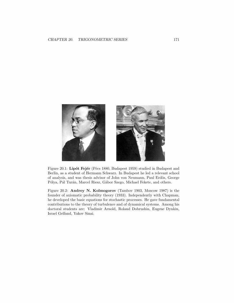
CHAPTER 20. TRIGONOMETRIC SERIES 171
Figure 20.1: Lipot Fejer (Pecs 1880, Budapest 1959) studied in Budapest andBerlin, as a student of Hermann Schwarz. In Budapest he led a relevant schoolof analysis, and was thesis advisor of John von Neumann, Paul Erdos, GeorgePolya, Pal Turan, Marcel Riesz, Gabor Szego, Michael Fekete, and others.
Figure 20.2: Andrey N. Kolmogorov (Tambov 1903, Moscow 1987) is thefounder of axiomatic probability theory (1933). Independently with Chapman,he developed the basic equations for stochastic processes. He gave fundamentalcontributions to the theory of turbulence and of dynamical systems. Among hisdoctoral students are: Vladimir Arnold, Roland Dobrushin, Eugene Dynkin,Israel Gelfand, Yakov Sinai.
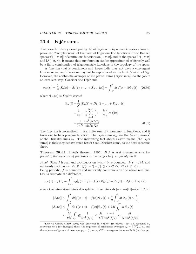
CHAPTER 20. TRIGONOMETRIC SERIES 172
20.4 Fejer sums
The powerful theory developed by Lipot Fejer on trigonometric series allows toprove the “completeness” of the basis of trigonometric functions in the Banachspaces C ([−π, π]) of continuous functions on [−π, π], and in the spaces L1(−π, π)and L2(−π, π). It means that any function can be approximated arbitrarily wellby a finite combination of trigonometric functions in the topology of the space.
A function that is continuous and 2π-periodic may not have a convergentFourier series, and therefore may not be reproduced as the limit N → ∞ of SN .However, the arithmetic averages of the partial sums (Fejer sums) do the job inan excellent way. Consider the Fejer sum
σN (x) =1
N[S0(x) + S1(x) + . . .+ SN−1(x)] =
∫ π
−π
dt f(x+ t)ΦN (t) (20.30)
where ΦN (x) is Fejer’s kernel:
ΦN (t) =1
N[D0(t) +D1(t) + . . .+DN−1(t)]
=1
2π+
1
π
N−1∑k=1
(1− k
N
)cos(kt)
=1
2πN
sin2(Nt/2)
sin2(t/2)(20.31)
The function is normalized, it is a finite sum of trigonometric functions, and itturns out to be a positive function. The Fejer sums σN are the Cesaro means5
of the Dirichlet sums Sk. The interesting fact about Cesaro means (the Fejersums) is that they behave much better than Dirichlet sums, as the next theoremsshow.
Theorem 20.4.1 (I Fejer theorem, 1905). If f is real continuous and 2π-periodic, the sequence of functions σn converges to f uniformly on R.
Proof. Since f is real and continuous on [−π, π] it is bounded, |f(x)| < M , anduniformly continuous: ∀ϵ ∃δ : |f(x+ t)− f(x)| < ϵ/2 ∀x, ∀t s.t. |t| < δ.Being periodic, f is bounded and uniformly continuous on the whole real line.Let us estimate the difference
σN (x)− f(x) =
∫ π
−π
dy[f(x+ y)− f(x)]ΦN (y) = J<(x) + J0(x) + J>(x)
where the integration interval is split in three intervals [−π,−δ)∪ [−δ, δ]∪ (δ, π].
|J0(x)| ≤∫ δ
−δ
dt|f(x+ t)− f(x)|ΦN (t) <ϵ
2
∫ δ
−δ
dtΦN (t) ≤ ϵ
2
|J>(x)| ≤∫ π
δ
dt|f(x+ t)− f(x)|ΦN (t) < 2M
∫ π
δ
dtΦN (t)
≤ M
πN
∫ π
δ
dt1
sin2(t/2)≤ M
πN
π − δ
sin2(δ/2)≤ M
N sin2(δ/2)
5Ernesto Cesaro (1859, 1906) was professor in Naples. He proved that if a sequence anconverges to a (or diverges) then: the sequence of arithmetic averages sn = 1
n
∑nk=1 ak and
the sequence of geometric averages pn = (a1 · · · an)1/n converge to the same limit (or diverge).
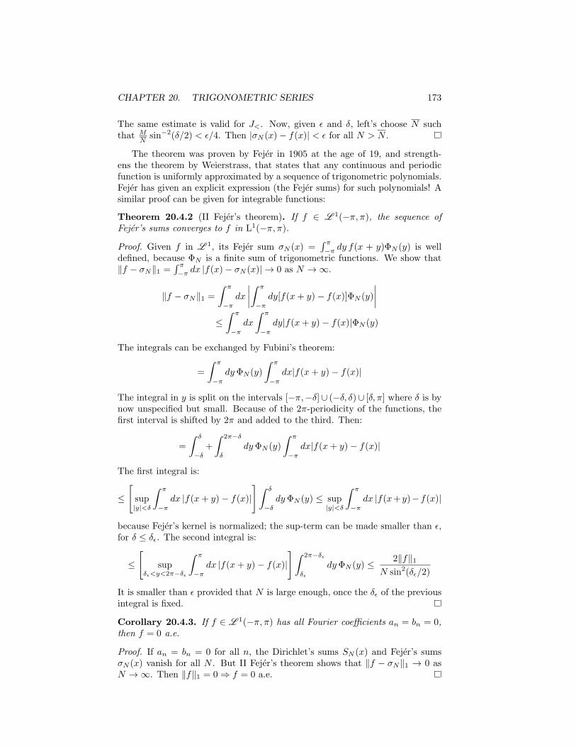
CHAPTER 20. TRIGONOMETRIC SERIES 173
The same estimate is valid for J<. Now, given ϵ and δ, left’s choose N suchthat M
Nsin−2(δ/2) < ϵ/4. Then |σN (x)− f(x)| < ϵ for all N > N .
The theorem was proven by Fejer in 1905 at the age of 19, and strength-ens the theorem by Weierstrass, that states that any continuous and periodicfunction is uniformly approximated by a sequence of trigonometric polynomials.Fejer has given an explicit expression (the Fejer sums) for such polynomials! Asimilar proof can be given for integrable functions:
Theorem 20.4.2 (II Fejer’s theorem). If f ∈ L 1(−π, π), the sequence ofFejer’s sums converges to f in L1(−π, π).
Proof. Given f in L 1, its Fejer sum σN (x) =∫ π
−πdy f(x + y)ΦN (y) is well
defined, because ΦN is a finite sum of trigonometric functions. We show that∥f − σN∥1 =
∫ π
−πdx |f(x)− σN (x)| → 0 as N → ∞.
∥f − σN∥1 =
∫ π
−π
dx
∣∣∣∣∫ π
−π
dy[f(x+ y)− f(x)]ΦN (y)
∣∣∣∣≤∫ π
−π
dx
∫ π
−π
dy|f(x+ y)− f(x)|ΦN (y)
The integrals can be exchanged by Fubini’s theorem:
=
∫ π
−π
dyΦN (y)
∫ π
−π
dx|f(x+ y)− f(x)|
The integral in y is split on the intervals [−π,−δ]∪ (−δ, δ)∪ [δ, π] where δ is bynow unspecified but small. Because of the 2π-periodicity of the functions, thefirst interval is shifted by 2π and added to the third. Then:
=
∫ δ
−δ
+
∫ 2π−δ
δ
dyΦN (y)
∫ π
−π
dx|f(x+ y)− f(x)|
The first integral is:
≤
[sup|y|<δ
∫ π
−π
dx |f(x+ y)− f(x)|
]∫ δ
−δ
dyΦN (y) ≤ sup|y|<δ
∫ π
−π
dx |f(x+y)−f(x)|
because Fejer’s kernel is normalized; the sup-term can be made smaller than ϵ,for δ ≤ δϵ. The second integral is:
≤
[sup
δϵ<y<2π−δϵ
∫ π
−π
dx |f(x+ y)− f(x)|
]∫ 2π−δϵ
δϵ
dyΦN (y) ≤ 2∥f∥1N sin2(δϵ/2)
It is smaller than ϵ provided that N is large enough, once the δϵ of the previousintegral is fixed.
Corollary 20.4.3. If f ∈ L 1(−π, π) has all Fourier coefficients an = bn = 0,then f = 0 a.e.
Proof. If an = bn = 0 for all n, the Dirichlet’s sums SN (x) and Fejer’s sumsσN (x) vanish for all N . But II Fejer’s theorem shows that ∥f − σN∥1 → 0 asN → ∞. Then ∥f∥1 = 0 ⇒ f = 0 a.e.
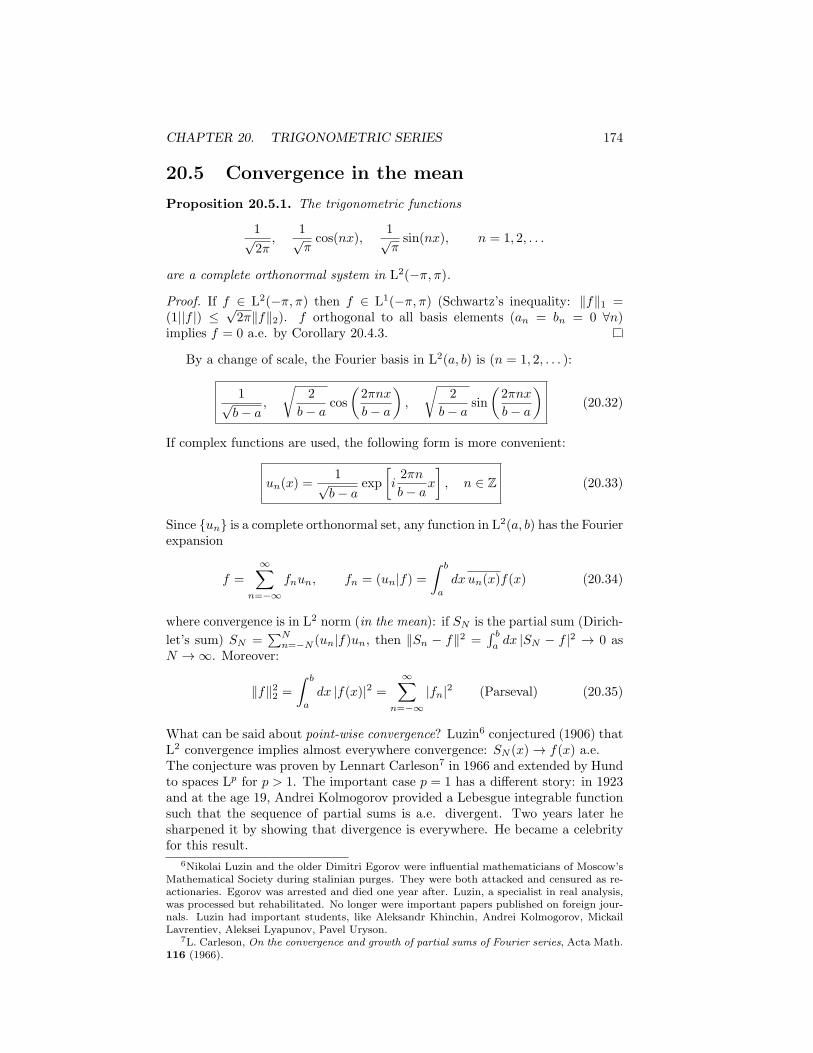
CHAPTER 20. TRIGONOMETRIC SERIES 174
20.5 Convergence in the mean
Proposition 20.5.1. The trigonometric functions
1√2π,
1√πcos(nx),
1√πsin(nx), n = 1, 2, . . .
are a complete orthonormal system in L2(−π, π).
Proof. If f ∈ L2(−π, π) then f ∈ L1(−π, π) (Schwartz’s inequality: ∥f∥1 =(1||f |) ≤
√2π∥f∥2). f orthogonal to all basis elements (an = bn = 0 ∀n)
implies f = 0 a.e. by Corollary 20.4.3.
By a change of scale, the Fourier basis in L2(a, b) is (n = 1, 2, . . . ):
1√b− a
,
√2
b− acos
(2πnx
b− a
),
√2
b− asin
(2πnx
b− a
)(20.32)
If complex functions are used, the following form is more convenient:
un(x) =1√b− a
exp
[i2πn
b− ax
], n ∈ Z (20.33)
Since un is a complete orthonormal set, any function in L2(a, b) has the Fourierexpansion
f =∞∑
n=−∞fnun, fn = (un|f) =
∫ b
a
dxun(x)f(x) (20.34)
where convergence is in L2 norm (in the mean): if SN is the partial sum (Dirich-
let’s sum) SN =∑N
n=−N (un|f)un, then ∥Sn − f∥2 =∫ b
adx |SN − f |2 → 0 as
N → ∞. Moreover:
∥f∥22 =
∫ b
a
dx |f(x)|2 =∞∑
n=−∞|fn|2 (Parseval) (20.35)
What can be said about point-wise convergence? Luzin6 conjectured (1906) thatL2 convergence implies almost everywhere convergence: SN (x) → f(x) a.e.The conjecture was proven by Lennart Carleson7 in 1966 and extended by Hundto spaces Lp for p > 1. The important case p = 1 has a different story: in 1923and at the age 19, Andrei Kolmogorov provided a Lebesgue integrable functionsuch that the sequence of partial sums is a.e. divergent. Two years later hesharpened it by showing that divergence is everywhere. He became a celebrityfor this result.
6Nikolai Luzin and the older Dimitri Egorov were influential mathematicians of Moscow’sMathematical Society during stalinian purges. They were both attacked and censured as re-actionaries. Egorov was arrested and died one year after. Luzin, a specialist in real analysis,was processed but rehabilitated. No longer were important papers published on foreign jour-nals. Luzin had important students, like Aleksandr Khinchin, Andrei Kolmogorov, MickailLavrentiev, Aleksei Lyapunov, Pavel Uryson.
7L. Carleson, On the convergence and growth of partial sums of Fourier series, Acta Math.116 (1966).
CHAPTER 20. TRIGONOMETRIC SERIES 175
20.6 From Fourier series to Fourier integrals
Consider the Fourier expansion of a function on the interval [−L2 ,
L2 ] :
f(x) =∞∑
k=−∞
ei2πkx/L
Lfk, fk =
∫ L/2
−L/2
dy e−i2πky/Lf(y)
where for convenience the two normalization factors√L are replaced by L in
the sum. In view of the limit L → ∞, introduce the new variable s = 2πk/L,with spacings δs = 2π/L:
f(x) =∑s
δseisx
2πf(s), f(s) =
∫ L/2
−L/2
dy e−isyf(y)
If f is integrable, the function f(s) exists for L→ ∞. If f is sufficiently regular,it does not change on the scale δs, and the sum may be replaced by an integral:
f(x) =
∫ ∞
−∞
ds
2πeisx
∫ ∞
−∞dy e−isyf(y)
According to this formula a function is a continuous superposition of Fouriercomponents, weighted by a function of the continuous index:
f(x) =
∫ ∞
−∞
ds√2πeisx(Ff)(s) (20.36)
(Ff)(s) =
∫ ∞
−∞
dy√2π
e−isyf(y) (20.37)
The second line defines the Fourier integral of f (the factors 2π are often dis-tributed differently).
Chapter 21
BOUNDED LINEAROPERATORS ONHILBERT SPACES
21.1 Linear functionals
The space of linear bounded functionals B(H ,C) is H ∗, the dual space of H .The inner product with a fixed vector (x|·) is a linear functional and is bounded,by Schwartz’s inequality. The following theorem proves that such functionalsexhaust all possibilities:
Theorem 21.1.1 (Riesz’s lemma). For each F ∈ H ∗ there is a uniquexF ∈ H such that Fx = (xF |x) for all x ∈ H . In addition ∥F∥ = ∥xF ∥.
Proof. If Ker F=H then xF = 0. If KerF is a proper subspace, then thereis a vector y orthogonal to it. Any vector x can be decomposed as x =(x − y Fx
Fy ) + y FxFy , where the first term belongs to KerF and then is orthog-
onal to y. The evaluation (y|x) = Fx (y|y)Fy shows that xF = y (Fy)∗
∥y∥2 . The vector
is unique, for suppose that Fx = (xF |x) = (x′F |x) for all x, then 0 = (xF −x′F |x)i.e. xF = x′F .Because of Schwarz’s inequality: |Fx| = |(xF |x)| ≤ ∥xF ∥∥x∥; equality is at-
tained at |FxF | = ∥xF ∥2. Therefore: ∥F∥ = supx|Fx|∥x∥ = ∥xF ∥.
Because of the identification of bounded functionals with vectors, Hilbertspaces are self-dual.
21.2 Bounded linear operators
The linear bounded operators with domain H and range in H form the Ba-nach space B(H ). The operator set is closed under the involutive action ofadjunction:
176
CHAPTER 21. BOUNDED LINEAROPERATORS ONHILBERT SPACES177
Theorem 21.2.1. For any linear operator A ∈ B(H ) there is an operatorA† ∈ B(H ) (the adjoint of A) such that:
(x|Ay) = (A†x|y) ∀x, y ∈ H (21.1)
and ∥A†∥ = ∥A∥.
Proof. Fix x ∈ H , the map y → (x|Ay) is a linear bounded functional. Then,by Riesz’ theorem, there is a unique vector v such that (x|Ay) = (v|y) for ally. The correspondence x → v is linear, i.e. it defines a linear operator on H :v = A†x.Equality of norms follows from Schwarz’s inequality and boundedness of A:|(A†x|y)| = |(x|Ay)| ≤ ∥x∥ ∥A∥∥y∥, if y = A†x then ∥A†x∥ ≤ ∥x∥∥A∥ i.e. A† isbounded and ∥A†∥ ≤ ∥A∥. The proof of equality is left to the reader.
Exercise 21.2.2. Show that:
(A+ B)† = A† + B†, (λA)† = λA†, (AB)† = B†A†, (A†)† = A.
Proposition 21.2.3. Let A ∈ B(H ), then Ker A is closed and
H = Ker A⊕ RanA† = Ker A† ⊕ RanA (21.2)
Proof. Suppose that xn is a sequence in Ker A, and xn → x. Then ∥Axn−Ax∥ ≤∥A∥∥xn − x∥ → 0 i.e. Ax = limn Axn = 0 i.e. x ∈ Ker A.Since Ker A is a closed linear subspace, it is H = KerA⊕ (KerA)⊥.
(RanA†)⊥ =x : (x|y) = 0 ∀y ∈ RanA†=x : (x|A†x′) = 0 ∀x′ ∈ H =x : (Ax|x′) = 0 ∀x′ ∈ H =x : Ax = 0 = KerA
Therefore (KerA)⊥ = RanA†. The second equality results after exchanging theoperators.
This statement is of practical utility. Consider the equation Ax = y; asolution x exists in H if y belongs to the range of A. Suppose that the rangeis a closed set; then y belongs to it if it is orthogonal to all vectors that solveA†x′ = 0.
If the equation Ax = λx has a nonzero solution x ∈ H , then λ and x arerespectively an eigenvalue and an eigenvector of A, and |λ| ≤ ∥A∥.
Exercise 21.2.4. Show that if A ∈ B(H ) is invertible with bounded inverse,then also A† is invertible with bounded inverse, and (A†)−1 = (A−1)†.
Definition 21.2.5. An operator A ∈ B(H ) is self-adjoint if A = A†:
(Ax|y) = (x|Ay), ∀x, y ∈ H
Theorem 21.2.6. The eigenvalues of a self-adjoint operator in B(H ) are real,and the eigenvectors corresponding to different eigenvalues are orthogonal.
CHAPTER 21. BOUNDED LINEAROPERATORS ONHILBERT SPACES178
Proof. Let x and x′ be eigenvectors corresponding to eigenvalues λ = λ′. From(Ax|x) = (x|Ax) one obtains λ = λ. From (Ax|x′) = (x|Ax′) one obtains(λ− λ′)(x|x′) = 0 i.e. x ⊥ x′ if λ = λ′.
Exercise 21.2.7. Show that if A is normal (i.e. AA† = A†A), then eigenvectorscorresponding to different eigenvalues of A are orthogonal.
Exercise 21.2.8. Let A ∈ B(H ); show that ∥A†A∥ = ∥A∥2.
Exercise 21.2.9. If A and B are bounded and self-adjoint then ∥AB∥ = ∥BA∥.
Exercise 21.2.10. Prove that if A is bounded and (x|Ax) = 0 ∀x, then A = 0(consider the expression 0 = (x+ λy|A(x+ λy)) for all λ, x, y).
Exercise 21.2.11. If A ∈ B(H ) and (x|Ax) is real for all x, then A = A†.
Exercise 21.2.12. Show that for a bounded and self-adjoint operator it is:
∥A∥ = sup∥x∥=1
|(x|Ax)| (21.3)
Hint: 4Re(x|Ay) = (x + y|A(x + y)) − (x − y|A(x − y)). Then 4|Re(x|Ay)| ≤sup∥w∥=1 |(w|Aw)|(∥x + y∥2 + ∥x − y∥2). Then use the parallelogram law, and set
x = Ay/∥Ay∥.
Exercise 21.2.13. Show that for a bounded operator it is:
12∥A∥ ≤ sup
∥x∥=1
|(x|Ax)| ≤ ∥A∥ (21.4)
Proposition 21.2.14. If A ∈ B(H ) is self-adjoint, then1:
A ≥ 0 ⇐⇒ (x|Ax) = maxy∈H
|(y|Ax)|2
(y|Ay)
If (y|Ay) = 0, then the quotient on the right-hand side is defined to be zero.
21.2.1 Integral operators
Linear integral operators are important, and arise for example in the study oflinear differential equations. Consider the inhomogeneous equation
f(x) = g(x) + λ
∫Ω
dy k(x, y)f(y),
where λ is a parameter, k is the kernel of the integral operator, g is assignedand f is the unknown function. In operator form it is f = g + λKf ,
(Kf)(x) =
∫Ω
dy k(x, y) f(y) (21.5)
The appropriate functional setting is suggested by the properties of the functiong and of the kernel k. A solution exists if g belongs to the range of 1− λK.
1A. G. Ramm, A variational principle and its application to estimating the electricalcapacitance of a perfect conductor, Am. Math. Monthly 120 n. 8 (2013) 743.
CHAPTER 21. BOUNDED LINEAROPERATORS ONHILBERT SPACES179
Let Ω be a bounded interval ([0, 1] for definiteness). If k ∈ L 2(Q) (Q isthe unit square) then K is a bounded operator on L2(0, 1): by Fubini’s theoremthe function y → |k(x, y)| is measurable and belongs to L 2(0, 1); by Schwarz’sinequality |(Kf)(x)| ≤ ∥k(x, ·)∥∥f∥2. Squaring and integration in x gives:
∥Kf∥2 ≤ ∥k∥ ∥f∥2
where ∥k∥2 =∫Qdxdy|k(x, y)|2. The adjoint operator is now evaluated2:
(h|Kf) =∫ 1
0
dxh(x)
[∫ 1
0
dy k(x, y)f(y)
]=
∫ 1
0
dy
[∫ 1
0
dxk(x, y)h(x)
]f(y) = (K†h|f)
(K†h)(x) =
∫ 1
0
dyk(y, x)h(y) (21.6)
The integral operator is self-adjoint if k(x, y) = k(y, x).Let us enquire about the solution of the integral equation (I − λK)f = g.
A solution exists if g ∈ Ran(I − λK) i.e. g ⊥ Ker(I − λK†). This means that gmust be orthogonal to the eigenvectors K†u = (1/λ)u.In particular, if |λ|∥K∥ < 1, it is both Ker (1−λK†) = 0 and Ker (1−λK) =0, and the operator (1− λK)−1 exists with domain H . The operator can beexpanded in a geometric series that converges for any g:
f = g + λKg + λ2K2g + . . .
The powers of the operator are integral operators with kernels k1(x, y) = k(x, y),
kn+1(x, y) =∫ 1
0du k(x, u) kn(u, y).
Example 21.2.15. Consider the integral equation
f(x) = g(x) +
∫ x
0
f(y)dy, a.e. x ∈ [0, 1], g ∈ L2(0, 1)
It corresponds to the Cauchy problem f ′ = f + g′ with f(0) = g(0). The kernelk(x, y) = θ(x − y) has L2 norm 1/
√2, therefore the iterative solution of the
integral equation converges, with kernels kn+1(x, y) = θ(x− y) (x− y)n/n!. Theconvergent Neumann series gives
f(x) = g(x) +
∫ x
0
dy ex−yg(y)
Example 21.2.16. In L2(0, 2π) (real functions) consider the equation
f = λKf + g, (Kf)(x) =
∫ 2π
0
dy sin(x+ y)f(y), λ ∈ R
2the steps are justified by Fubini’s theorem for the exchange of order of integration: letf(x, y) be measurable on M×N , then
∫M dm(
∫N dm|f |) < ∞ iff
∫N dm(
∫M dm|f |) < ∞ and,
if they are finite it is: ∫M
dm
(∫N
dmf
)=
∫N
dm
(∫M
dmf
)
CHAPTER 21. BOUNDED LINEAROPERATORS ONHILBERT SPACES180
It is (Kf)(x) = f1 sinx + f2 cosx, where f1 =∫dx cos(x)f(x) and f2 =∫
dx sin(x)f(x). The operator K is rank 2 and self-adjoint. The problem isthen two-dimensional and the solution, if existent, has the form:
f(x) = λ(f1 sinx+ f2 cosx) + g(x)
By taking the inner products with cosx and sinx we get:[1 −λπ
−λπ 1
] [f1f2
]=
[g1g2
]where g1 = (cos |g) and g2 = (sin |g) The solution exists for any g and is uniqueif 1− λ2π2 = 0. Once f1 and f2 are evaluated, it is:
f(x) = g(x) + λ
∫ 2π
0
dysin(x+ y) + λπ cos(x− y)
1− λ2π2g(y)
If λ = 1/π, a solution exists if g ∈ Ran(I − 1π K) i.e. g ⊥ Ker(I − 1
π K) (K is
self-adjoint). The set Ker contains the solutions of the equation: Ku = πu. Up
to a pre-factor it is: u(x) = sinx + cosx. Then:∫ 2π
0dx(sinx + cosx)g(x) = 0
and the solution is f(x) = c(sinx+cosx)+g(x) where c is an arbitrary constant.The case λ = −1/π is treated similarly.
Exercise 21.2.17. Show that the following linear operator belongs to B(L2(R))and it is self-adjoint:
(T f)(x) =
∫ ∞
−∞dy
f(y)
x2 + y2 + 1
(note that it is not invertible, as all odd-parity functions belong to the kernel).
21.2.2 Orthogonal projections
Given a closed subspace M and a vector x, the projection theorem states thatx = p + w, where p ∈ M and w ∈ M⊥, and the decomposition is unique.Therefore the projection operator on M , P (M) : x → p, is well defined. Forshort we write P for P (M).
Proposition 21.2.18. The orthogonal projector P is linear, self-adjoint, andidempotent (P 2 = P ).
Proof. Let x = p+w and x′ = p′+w′, then αx+βx′ = (αp+βp′)+(αw+βw′),where αp + βp′ ∈ M and αw + βw′ ∈ M⊥, ∀α, β. As the decomposition isunique, necessarily it is P (αx+ βx′) = αp+ βp′ = αPx+ βPy.(x − P x|y − P y) = (x − P x|y) (because x − P x is orthogonal to M), and foranalogous reason (x− P x|y − P y) = (x|y − P y); then (P x|y) = (x|P y).P 2x = P p = p = P x, then P 2 = P .
It turns out that these properties uniquely characterise an orthogonal pro-jection operator. It is convenient to reverse the approach and introduce suchoperators through the definition:
Definition 21.2.19. An orthogonal projection operator is a linear operator onH such that: P 2 = P , P † = P .
CHAPTER 21. BOUNDED LINEAROPERATORS ONHILBERT SPACES181
Remark 21.2.20.1) The closed subspace where vectors are projected is M = RanP .2) Let y = x− P x, then P y = 0 and (y|P x) = 0 ∀x , i.e. KerP (M) =M⊥.3) Since ∥x∥2 = ∥P x + y∥2 = ∥P x∥2 + ∥y∥2 ≥ ∥P x∥2, it follows that ∥x∥ ≥∥P x∥, with equality holding for x ∈ M . Then ∥P∥ = 1. Being bounded, P iscontinuous.4) A projector P (M) has only the eigenvalues 1 and 0, with eigenspaces M andM⊥, M ⊕M⊥ = H .
Examples: 1) In L2(R) the multiplication operator f → χ[a,b]f , where χ[a,b] isthe characteristic function of an interval [a, b], is an orthogonal projector. Theinvariant subspace M is given by functions that vanish a.e. for x /∈ [a, b].2) The operators (P±f)(x) =
12 [f(x)± f(−x)] are orthogonal projectors on the
orthogonal subspaces of (a.e.) even and odd functions.
Exercise 21.2.21. Let P (M) and P (M ′) be projectors, then:1) P (M) + P (M ′) is a projector iff M ⊥ M ′. In this case P (M) + P (M ′) =P (M ⊕M ′).2) P (M)P (M ′) is a projector iff P (M) and P (M ′) commute. In this caseP (M)P (M ′) = P (M ∩M ′).
Exercise 21.2.22. Let x1 . . . xn be linearly independent vectors in a Hilbertspace. Write the projection operator on the linear subspace spanned by the nvectors.Solution: P y =
∑ij xi[G
−1]ij(xj |y), where Gij = (xi|xj) is Gram’s matrix.
Exercise 21.2.23. Let (DNf)(x) =∫ 2π
0dyDN (x− y)f(y), where DN (x) is the
Dirichlet kernel (20.6), and f ∈ L 2(0, 2π). What is the operator norm of DN?Is it true that limN→∞DN = I in the operator norm?
21.2.3 The position and momentum operators
On L2[a, b] define the “position” operator that multiplies a function f by thefunction x (x(t) = t): Qf = xf i.e. (Qf)(t) = tf(t).The operator is bounded, ∥Qf∥ ≤ max(|a|, |b|) ∥f∥, and it is self-adjoint:
(g|Qf) =∫ b
a
dt g(t)t f(t) =
∫ b
a
dt tg(t)f(t) = (Qg|f).
The eigenvalue equation Qf = λf has no solution in L2[a, b]: the equation(t − λ)f(t) = 0 a.e. t ∈ [a, b] implies that f = 0 a.e. We may ask if there are“approximate eigenfunctions”: ∥Qu − λu∥ < ϵ∥u∥. Consider the normalizedfunctions uη = 1√
2ηχ[λ−η,λ+η] and evaluate
∥Quη − λuη∥2 =
∫ b
a
dt(t− λ)2uη(t)2 =
η2
3→ 0
However, the limit η → 0 of uη does not exist in Hilbert space3.
3the functions do not form a Cauchy sequence: for δ < η it is ∥uη − uδ∥2 = 2(1−√
δ/η)which may not be small as η, δ → 0.
CHAPTER 21. BOUNDED LINEAROPERATORS ONHILBERT SPACES182
A function f is absolutely continuous on [a, b], AC[a, b], if there is a functionh ∈ L 1(a, b) such that:
f(x) = f(a) +
∫ x
a
dx′h(x′), x ∈ (a, b).
The functions in AC[a, b] are continuous and differentiable. They form a linearsubset in L p(a, b) for all p. By the theorem of the mean: f ′(x) = h(x).The derivative is the linear “momentum” operator4
(P f)(x) = −if ′(x) (21.7)
with domain on AC[a, b] functions such that f ′ ∈ L 2(a, b). If f1 and f2 areAC[a, b], integration by parts gives:
(f1|P f2) = −i∫ b
a
dxf1(x)f′2(x) = −if1f2
∣∣∣ba+ (P f1|f2).
The operator is symmetric provided that the boundary terms cancel. Thisis achieved if the domain of P is restricted to AC functions with appropriateboundary conditions (b.c.): f(b) = f(a) = 0 (Dirichlet b.c.), or f(b) = ±f(a)(periodic/antiperiodic b.c.) or f(b) = eiθf(a) (Bloch b.c. with θ ∈ R). Theyproduce three different definitions of P (same action but different domains whereit is symmetric).
21.3 Unitary operators
Definition 21.3.1. A linear operator U with domain H and range in H is anisometry if ∥Ux∥ = ∥x∥ for all x. If also Ran U = H the operator is unitary.
1) The conservation of the norm implies that Ker U = 0 i.e. U−1 exists and
(Ux|Uy) = (x|y) ∀x, y (21.8)
2) The operator is bounded with norm ∥U∥ = 1.3) (x|y) = (Ux|Uy) = (U†Ux|y) ∀x, y, then U†Ux = x for all x i.e.
U†U = I (21.9)
Therefore, U† = U−1, and it is a unitary operator: ∥x∥ = ∥U(U†x)∥ = ∥U†x∥for all x.4) If λ is an eigenvalue of U , then |λ| = 1. Eigenvectors with different eigenvaluesare orthogonal.5) The product of unitary operators is unitary.
Exercise 21.3.2. If U and V are unitary then ∥U AV ∥ = ∥A∥ ∀A ∈ B(H ).
Exercise 21.3.3. Let H ∈ B(H ) be self-adjoint. Show that the Cayley trans-form of H, (1− iH)(1+ iH)−1, is well defined and is a unitary operator. Whatis the Cayley transform of a projector?
4physicists introduce Planck’s constant, P f = −iℏf ′.
CHAPTER 21. BOUNDED LINEAROPERATORS ONHILBERT SPACES183
Exercise 21.3.4. Show that if H is bounded and self-adjoint, the operators
Ut = e−itH , t ∈ R, are unitary and form a group. H is the generator of thegroup (see Sect.18.5.3).
Exercise 21.3.5. P is a projector; evaluate eiθP and (z − P )−1 (z = 0, 1).
21.4 Notes on spectral theory
Definition 21.4.1.Discrete spectrum: z ∈ σp(A) if z is an eigenvalue:
∃u ∈ H such that Au = zu
i.e. Ker(z − A) = 0 i.e. (z − A)−1 does not exist.Continuous spectrum: z ∈ σc(A) if z is a generalized eigenvalue:
z /∈ σp(A), ∃un ⊂ H , ∥un∥ = 1, such that limn→∞
∥Aun − zun∥ = 0.
Remark 21.4.2.1) If A = A†, then σp(A) ⊆ R.2) Continuous spectrum: un is not a Cauchy sequence. Convergence un → uand continuity of A would imply that u is an eigenvector and z ∈ σp(A).
3) If z ∈ σc(A) the operator (z − A)−1 exists, but it cannot belong to B(H ).Proof: Suppose that it does (then the domain is H and it is bounded):
1 = |(un|(z − A)−1(z − A)un)| ≤ ∥(z − A)−1∥∥zun − Aun∥
since for n→ ∞ the last factor is zero, the other factor cannot be finite.It turns out that either (z − A)−1 has domain H without being bounded, or itsdomain is strictly contained in H .4) Since |(un|(A − λ)un)| ≤ ∥Aun − λun∥, it is λ = limn→∞(un|Aun). Then,for self-adjoint operators, it is σc(A) ⊆ R and |λ| ≤ ∥A∥ (use continuity of themodulus).
5) If z ∈ σc(A) then z ∈ σc(A†) and 0 = Ker (z − A†) = Ran (z − A) i.e.
H = D (z − A)−1. Therefore, either D(z− A)−1 = H (but the resolvent is notbounded) or D(z − A)−1 is a proper subset, but dense.
For a bounded operator, the set σ = σp∪σc is the spectrum of the operator.In summary, if z ∈ σ the following occurs: ∀ϵ > 0 ∃uϵ ∈ H such that ∥(z −A)u∥ ≤ ϵ∥u∥. If z /∈ σ(A) the resolvent (z − A)−1 exists and it is bounded.
Chapter 22
UNITARY GROUPS
The stage for quantum mechanics is the Hilbert space; continuous symmetriesare main actors in the play, and correspond to unitary operators1. Of specialimportance are groups (subgroups) that depend continuously on one parameter,like rotations around a given axis, or translations along a given direction. Theycorrespond to special families of unitary operators. The following theorems arevery important and useful (they are stated without proof2).
22.1 Stone’s theorem
Definition 22.1.1. A family of unitary operators Us, s ∈ R, is a stronglycontinuous one-parameter unitary group if:
UsUs′ = Us+s′
lims→0
∥Usx− x∥ = 0 ∀x ∈ H .
It is clear that the group is Abelian, U0 = I and U−1s = U−s. For such groups,
the following fundamental theorem holds:
Theorem 22.1.2 (Stone’s theorem). Let Us be a strongly continuous one-parameter unitary group on a Hilbert space. Then there is a self-adjoint operatorH such that
Us = e−isH (22.1)
H is the generator of the group, with domain
D(H) = x ∈ H such that lims→0
Usx− x
−isexists,
Hx is precisely the above limit.
1Discrete symmetries may correspond also to anti-unitary (i.e. antilinear and norm con-serving) operators. An example is time-reversal.
2see for example: K. Schmudgen, Unbounded Self-adjoint Operators on Hilbert Space,Springer 2012.
184
CHAPTER 22. UNITARY GROUPS 185
Theorem 22.1.3 (Lie-Trotter formula). Let A and B be self-adjoint opera-tors. If A+ B is self-adjoint on D(A) ∩ D(B), then:
eit(A+B)x = limn→∞
[eitA/neitB/n
]nx (22.2)
22.2 Weyl operators
Two important families of unitary operators on L2(Rn) are:translations by vectors a ∈ Rn:
(Uaf)(x) = f(x− a), UaUa′ = Ua+a′ (22.3)
multiplication by a phase factor with vector p ∈ Rn:
(Vpf)(x) = e−iℏ p·xf(x), VpVp′ = Vp+p′ (22.4)
Planck’s constant ℏ is here introduced to give x, a the physical dimension oflength, and p the dimension of momentum.The translations along a fixed direction Uan, a ∈ R, and phase multiplicationsVpn, p ∈ R, are strongly continuous one-parameter unitary groups. Stone’stheorem implies the existence of self-adjoint generators.On the dense set of square-integrable analytic functions, a Taylor expansiongives:
(Uanf)(x) = f(x− an) = f(x) + (−an · ∇)f(x) + 12! (−an · ∇)2f(x) + . . .
Therefore, the generator of translations with direction n is the self-adjoint op-erator whose restriction to analytic functions is −iℏ n · ∇ =
∑i niPi, and
Ua = exp
[− i
ℏa · P
], Pkf = −iℏ ∂f
∂xk
Pk is the generator of translations along the direction k. Momentum operatorsare self-adjoint on a dense domain in L2(Rn) and act as derivatives on thesubset of analytic functions. The property UaUa′ = Ua′Ua for all vectors a anda′ implies, for infinitesimal vectors, the relation [Pi, Pj ] = 0.
The generator of the one-parameter group (Vpnf)(x) = exp(− iℏpn · x)f(x)
is the (unbounded) self-adjoint operator n · Q, and
Vp = exp
[− i
ℏp · Q
], (Qif)(x) = xif(x).
The n operators Qi are self-adjoint and commute on a dense domain in L2(Rn).The generators Qi and Pi i = 1 . . . n form Heisenberg’s algebra:
[Qi, Qj ] = 0, [Pi, Pj ] = 0, [Qi, Pj ] = iℏδij
The first two commutation relations correspond to the fact that the unitarygroups are Abelian. The mixed commutator, proportional to the identity oper-ator, reflects a simple relation among the groups (Weyl’s commutation relation):
Vp Ua = eiℏ p·a Ua Vp (22.5)
CHAPTER 22. UNITARY GROUPS 186
Proof. (VpUaf)(x) = eiℏ p·x(Uaf)(x) = e
iℏ p·xf(x− a) = e
iℏ p·a(Vpf)(x− a)
= eiℏ p·a(UaVpf)(x).
Exercise 22.2.1. Show that the translation operator (Uaf)(x) = f(x− a) doesnot have eigenvectors in L2(R). (Hint: a periodic function cannot be integrable).
Exercise 22.2.2. Let [A, B] = iI, A = A† and B = B†. Show that A and Bcannot be both bounded.Sketch of the proof: suppose that A and B are bounded, then [An, B] = inAn−1
and [exp(−itA), B] = t exp(−itA); conclude that ∥B∥ is larger that any realnumber.
Exercise 22.2.3 (Scale transformations). On L2(R) the operators
(Dλf)(x) = e−λ/2f(e−λx), λ ∈ R (22.6)
are a strongly continuous one-parameter unitary group. On the dense subspaceS (R) (see chapter on Schwartz space):1) obtain the generator D = 1
2 (QP + P Q) i.e. Dλ = exp(−iλD);
2) show that D†λQDλ = eλQ and D†
λP Dλ = e−λP .
Scale transformations are related to theVirial property. This is illustratedfor the anharmonic oscillator, H = 1
2m P2 + 1
2kQ2 + bQ4 (b > 0).
Let Hψ = Eψ, then E = 12m ⟨P 2⟩+ 1
2k⟨Q2⟩+ b⟨Q4⟩, where E = ⟨H⟩ = (ψ|Hψ)
etc. are the average values. The action of a scale transformation is: ⟨D†λHDλ⟩ =
e−2λ 12m ⟨P 2⟩+ e2λ 1
2k⟨Q2⟩+ be4λ⟨Q4⟩. The linear term of an expansion in small
λ is: i(ψ|[D, H]ψ) = −2 12m ⟨P 2⟩+2 1
2k⟨Q2⟩+4b⟨Q4⟩. Since the left hand side is
zero for an eigenvector, an identity is obtained among terms that contribute tothe total energy. If b = 0, one gets the equality of kinetic and potential energyterms of the harmonic oscillator, ⟨ 1
2m P2⟩ = ⟨ 12k
2Q2⟩, that is used, for example,in the theory of specific heats.
22.3 Space rotations, SO(3)
Space rotations act on vectors in R3 as 3 × 3 real matrices R that preservelengths, RRt = I3, and orientation, detR = 1. They form the group SO(3).Being unitary, rows or colums of R are orthogonal and normalized, eigenvaluesare on the unit circle.The characteristic polynomial det(zI3 −R) is real cubic, then it necessarily hasa positive real zero (equal to one) corresponding to a real eigenvector of R: theinvariant vector Rn = n.The other two eigenvalues may be 1, 1 or −1,−1 (then R is the identity matrixor a diagonal matrix describing two reflections) or e±iφ with eigenvectors u± ivmaking with n an orthogonal set in C3. This implies that the vectors n, u andv are orthogonal in R3. Note that trR = 1 + 2 cosφ.The eigenvalue equation R(u± iv) = e±iφ(u± iv) i.e. the pair
Ru = u cosφ− v sinφ
Rv = u sinφ+ v cosφ
CHAPTER 22. UNITARY GROUPS 187
shows that two vectors rotate under the action of R in the plane perpendicularto n. For the rotation to be anticlockwise, the orientation n = v × u is chosen.Every vector x can be expanded in the orthonormal basis: x = xnn+xuu+xv vwhere xn = x · n etc. The action of R is:
Rx =xnn+ xu(u cosφ− v sinφ) + xv(u sinφ+ v cosφ)
=xnn+ (xuu+ xv v) cosφ+ (xvu− xuv) sinφ
=xnn+ (x− xnn) cosφ+ n× x sinφ
= x cosφ+ (1− cosφ)(n · x)n+ n× x sinφ
Exercise 22.3.1. Write the rotation as a matrix on the column vector (x, y, z)t.
The invariant unit vector n that identifies the rotation axis and the rota-tion angle φ measured anticlockwise, are a useful parameterization of rotations.We’ll soon discover that the parameters n and φ combine in a vector n φ.The expansion for an infinitesimal angle provides the neighborhood of the iden-tity matrix, which is extremely instructive in the study of groups with analyticdependence on parameters (Lie groups):
Rx = x+ n× x δφ + . . . = (I3 + δφA+ . . .)x
A =
0 −n3 n2n3 0 −n1−n2 n1 0
= n · A (22.7)
A1 =
0 0 00 0 −10 1 0
, A2 =
0 0 10 0 0−1 0 0
, A3 =
0 −1 01 0 00 0 0
The rotations with same invariant vector form a commutative subgroup:
R(nφ1)R(nφ2) = R(n(φ1 + φ2)) (22.8)
If one angle is infinitesimal: R(nφ)(I3 + δφ n · A+ . . . ) = R(n(φ+ δφ)). Sincethe factors can be exchanged, one concludes that the matrices of the subgroupR(nφ) commute with n · A (then, they have the same eigenvectors). Moreover,by taking the limit δφ to zero:
d
dφR(nφ) = (n · A)R(nφ) (22.9)
with the initial condition R(0) = I3. Since factors commute, the solution is
R(nφ) = eφ n·A (22.10)
The matrix n · A is the generator of rotations along the direction n. The threematrices Ai are the generators along the three coordinate directions, and are abasis for antisymmetric matrices.Real antisymmetric matrices form a linear space that is closed under the oper-ation A,A′ → [A,A′]. The commutator is a Lie product3, and the linear space
3In a linear space X, a Lie product is a bilinear map ∗ : X ×X → X such that x ∗ x = 0,x ∗ y = −y ∗ x, (x ∗ y) ∗ z + (y ∗ z) ∗ x+ (z ∗ x) ∗ y = 0 (Jacobi property).
CHAPTER 22. UNITARY GROUPS 188
with Lie product is the Lie algebra so(3) of the SO(3) group. Because Ai are abasis, the Lie product of two basis matrices is expandable in the basis itself,
[Ai, Aj ] = ϵijkAk (22.11)
The coefficients4 ϵijk are the structure constants of so(3) and are typical of therotation group.Let z3+az2+bz+c = 0 be the characteristic polynomial det(z I3−M) of a 3×3matrix M ; Cayley-Hamilton’s theorem states that M3 + aM2 + bM + cI3 = 0.The theorem implies that it is possible to expand the exponential of a 3 × 3matrix into a sum of powers:
R = eφ(n·A) = α I3 + β(n · A) + γ(n · A)2
If the identity is acted on the three eigenvectors of R (that are also eigenvectors
of (n · A) with eigenvalues 0, ±i) a linear system is obtained: 1 = α, e±iφ =α± iβ−γ. The coefficients are evaluated and one re-obtains the explicit generalform of a rotation matrix:
R(nφ) = I3 + sinφ(n ·A) + (1− cosφ)(n · A)2 (22.12)
Each rotation is identified by a vector nφ in the ball of radius π. A diametercorresponds to the subgroup of rotations with same rotation axis; the two op-posite points ±nπ at the surface give the same rotation and must be identified.The diameter is then a circle, the center of the sphere is the unit of the group.Therefore, the manifold of parameters is a sphere with opposite points at thesurface being identified (a bundle of circles through the origin). The identifi-cation makes the manifold doubly connected: two rotations (two points A, Bof the manifold) may be connected by two inequivalent paths (one path cannotbe continuously deformed into the other). A choice is: the chord AB, the paththat joins A to the surface at a point C = C′ (antipode) and continues to B.
Example 22.3.2. Find the angle and the invariant vector of the rotation
R = eA , A =
0 3 1−3 0 −5−1 5 0
.Note that A = −At is normal and shares with R the same eigenvectors. There-fore if z is an eigenvalue of A, ez is an eigenvalue of R. The invariant vectorsolves An = 0 i.e. 0 3 1
−3 0 −5−1 5 0
n1n2n3
= 0 ⇒ n = ± 1√35
51−3
(22.13)
The eigenvalues of A solve 0 = det(zI3 − A) = z3 + 35z. They are 0, ±i√35.
The angle of rotation is therefore√35 radiants (mod. 2π).
Since the rotation angle is positive if anticlockwise with respect to the direction
4ϵ123 = 1 and cyclic, ϵ213 = −1 and cyclic, zero otherwise. Note that the vector productof two real vectors is (a× b)i = ϵijkajbk.
CHAPTER 22. UNITARY GROUPS 189
of n, we must decide the sign of n. This can be done by checking the infinites-imal rotation of a conveniently chosen vector: a rotation with same axis butinfinitesimal angle is I3 +
ϵ√35A + . . . . The vector v = (0, 0, 1)t transforms to
v + δv where
δv =ϵ√35
1−50
= ϵ n× v
provided that n is chosen with the upper sign in (22.13).
22.3.1 SU(2)
More fundamental than SO(3) for the theory of rotations is the group SU(2) ofunitary 2× 2 complex matrices, U†U = I with detU = 1:
U =
[z −ww z
], |z|2 + |w|2 = 1 (22.14)
The parameters span the surface of the unit sphere in R4, which has no bound-ary, and is simply connected. Another parameterization of SU(2) is obtainedby solving the constraints:
U(nφ) = cosφ
2− in · σ sin
φ
2(22.15)
σi are the Pauli matrices. It is simple to check that the expression correspondsto the exponential representation:
U(nφ) = e−i2φn·σ (22.16)
The generators σi/2 are a basis for traceless Hermitian 2 × 2 matrices, whichis the Lie algebra su(2) of SU(2), with Lie product H,H ′ → −i[H,H ′]. Thestructure constants are the same of su(3):
−i[σi2,σj2
]= ϵijk
σk2
(22.17)
The exponential map takes the Lie algebra to the Lie group:
exp : su(2) → SU(2).
Despite the diversity of SO(3) and SU(2), their exponential representations areformally identical: only a replacement of the basis matrices changes one intoanother, the structure constants being the same.Now the parameter space is the ball in R3 of radius 2π. However, all “surface”points correspond to the single matrix of inversion: U(±n 2π) = −1. Therefore,the manifold is a bundle of circles (the diameters are the one parameter sub-groups) with points (matrices) ±n 2π in common.This parameter space, or the surface of the unit sphere in R4 (|z|2 + |w|2 = 1)are simply connected manifolds: this makes SU(2) more fundamental (coveringgroup) than SO(3).
Exercise 22.3.3. Show that U†σU = Rσ, R ∈ SO(3). Therefore ±U corre-spond to the same R matrix.
CHAPTER 22. UNITARY GROUPS 190
22.3.2 Representations
From the point of view of physics, space rotations are a subgroup of the Galileiand of the Lorentz groups of symmetries for physical laws.An observer O is specified by an orthonormal frame ek, which can be identifiedmaterially by rigid rulers for measuring positions, at right angles at a point (theorigin). A rotated observer O′ is an orthonormal frame e′k with same originand orientation. A point P has coordinates x′k linked by a rotation matrix tothe coordinates measured by O: x′k = Rkjxj .Suppose that O and O′ measure in every point some quantity (a field). In thesimplest case the quantity is a number (a scalar) that is a property of the point.They measure two scalar fields f and f ′, and the values of the two fields at thesame physical point P (of coordinates x and x′) must be the same:
f(x) = f ′(x′), i.e. f ′(x) = f(R−1x) (22.18)
If they measure a vector field (for example a force field), they measure a physicalarrow at each point. Since they use rotated frames, the components of the arrowat a point are different:∑
k
Vk(x)ek =∑k
V ′k(x
′)e′k, ⇒ V ′k(x) = RkjVj(R
−1x) (22.19)
The two laws describe the transformation of a scalar field and a vector field underrotations. A spinor 1/2 field is a two component complex field that transformswith a SU(2) rotation:
ψ′a(x) = U(R)abψb(R
−1x) (22.20)
If the (scalar, spinor, vector or whatever) fields F and F ′ measured by Oand O′ are thought of as points in the same functional space, the rotationof coordinates R induces a map UR : F → F ′. Since fields can be linearlycombined, the map is asked to be linear. Moreover, if two rotations R and R′
are done in the order, the observer O′′ is linked to O by x′′ = R′Rx, and thusF ′′ = UR′RF i.e. maps form a linear representation of the rotation group:
UR′R = UR′UR (22.21)
Let us consider some relevant cases.
Think of a scalar field f as a “point” in L2(R3). A rotation induces thelinear map f ′ = URf defined by (URf)(x) = f(R−1x). The operators UR are
unitary because Lebesgue’s measure is rotation invariant, then UR−1 = U†R.
The rotations with fixed direction n correspond to a commutative subgroupparameterized by the angle: Un(φ)Un(φ
′) = Un(φ + φ′) (they are a stronglycontinuous one-parameter group). By Stone’s theorem there is a self-adjoint
(unbounded) generator such that Un(φ) = e−iℏφL(n). The self-adjoint opera-
tor L(n) is the generator of the one parameter group, and corresponds to theprojection along n of the orbital angular momentum. A simpler approach is to
CHAPTER 22. UNITARY GROUPS 191
restrict to the set of analytic functions and consider an infinitesimal rotation:
(Un(δφ)f)(x) =f(x− δφ n× x+ . . .)
=f(x)− δφ (n× x)k∂f
∂xk(x) + . . .
=f(x)− i
ℏδφ n · (Lf)(x) + . . .
L = Q× P (22.22)
The three operators Lx, Ly and Lz satisfy the Lie algebra
1
iℏ[Li, Lj ] = ϵijkLk (22.23)
and generate the unitary subgroups representing rotations around the three co-
ordinate axis. For the axis n it is L(n) = n · L.
For a 1/2 spinor field, the expansion near unity of (22.20) gives
[U(n δφ)ψ]a(x) =
[I − iδφ n · σ
2+ . . .
]ab
(I − i
ℏδφ n · L+ . . .
)ψb(x)
= ψa(x)−i
ℏδφ (n · J)abψb(x) + . . .
σkab are the components of the Pauli matrix σk. The generator is the projection of
the total angular momentum, which is the vector sum of spin and orbital angularmomentum operators, acting independently on spin variables (components a, b)and on position variables:
J = S + L (22.24)
where S = ℏ2 σ are the spin operators (matrices) for spin 1/2 particles.
Also in this case the algebra is that of angular momentum (rotation group):
1
iℏ[Ji, Jj ] = ϵijkJk. (22.25)
Exercise 22.3.4. Show that [J2, Ji] = 0, where J2 =∑
i J2i .
Chapter 23
UNBOUNDED LINEAROPERATORS
Many operators of interest are unbounded, and are defined on a subset of theHilbert space. The domain (D), the range (Ran) and the kernel (Ker) of alinear operator are linear subspaces. If the kernel contains only the null vectorthe operator is injective and the inverse operator exists (and is linear).
23.1 The graph of an operator
The graph of a real function f is the set (x, y) in R2, where x is in the domain off and y = f(x). A very useful tool is the graph of a linear operator, introducedby Von Neumann:
Definition 23.1.1. The graph of a linear operator is the set
G(A) = (x, y) : x ∈ D(A), y = Ax (23.1)
It is a subset of H 2 = H ×H , with elements X = (x, y). H 2 is a linear spacewith the rules λX = (λx, λy) and X+X ′ = (x+x′, y+ y′), and a Hilbert spacewith inner product
(X|X ′) = (x|x′) + (y|y′).The norm is ∥X∥2 = ∥x∥2 + ∥y∥2. Completeness is readily proven: if Xn isa Cauchy sequence, ∥Xn − Xm∥2 = ∥xn − xm∥2 + ∥yn − ym∥2 < ϵ for alln,m > Nϵ, then xn and yn are separately Cauchy sequences and then convergeto x and y. The pair X = (x, y) is the limit of Xn in H 2: ∥Xn − X∥2 =∥xn − x∥2 + ∥yn − y∥2 → 0.
The graph is a linear subspace in H 2. Conversely, a linear subspace S isthe graph of a linear operator if (x, y) ∈ S and (x, y′) ∈ S imply y = y′ (theassignment x→ y is unique). This is equivalent to: (0, y) ∈ S ⇒ y = 0.
If the inverse of the operator A exists, its graph is
G(A−1) = (y, x) : (x, y) ∈ G(A) (23.2)
Definition 23.1.2. A linear operator A′ is an extension of a linear operator Aif G(A) ⊂ G(A′) (in other words: D(A) ⊂ D(A′) and A′ = A on D(A)).
192
CHAPTER 23. UNBOUNDED LINEAR OPERATORS 193
23.2 Closed operators
A graph is a closed set if every Cauchy sequence Xn in the graph converges to apoint X in the graph (a Cauchy sequence Xn is convergent, by the completenessof H 2; the point is that the limit X must be in the graph).
Definition 23.2.1. A linear operator A is closed if its graph is a closed set.
This definition is an example of how useful the concept of graph is. Withoutit, the definition is: A is closed if ∀xn in D(A) such that xn → x and Axn → y⇒ x ∈ D(A) and y = Ax.
Remark 23.2.2.1) “A is closed” does not mean that D(A) is closed nor that A is continuous:it only means that D(A) contains the limit points of convergent sequences suchthat also the sequence Axn converges, and converges to the image of the limitpoint (the graph is very useful to visualize this).2) If A is closed, Ker A is a closed subspace.3) The inverse of a closed linear operator, is closed.
If the graph G(A) of a linear operator is not closed, the set can be always
extended to its closure G(A) by adding the frontier. The closure is still a linearsubspace1 and it is the smallest closed extension of the set. However, it mightnot be a graph of a linear operator, as it may fail to have the property (0, y) ∈G(A) ⇒ y = 0.
Definition 23.2.3. If G(A) is the graph of a linear operator A, the operator A is
the closure of A, and it is the minimal closed extension of A. It is G(A) = G(A).
Proposition 23.2.4. If G(A) is not a graph of a linear operator, then A hasno closed extensions.
Proof. If G(A) is not a graph, it contains a point (0, y) with y = 0. Suppose
that A has a closed extension Ac; then G(A) is necessarily a proper subset ofG(Ac). But if (0, y) ∈ G(Ac), the set cannot be the graph of an operator.
The property of being a closed operator is important. In this presentationit will be a prerequisite for the introduction of the spectrum.
23.3 The adjoint operator
Let us enquire about the existence of the adjoint operator. According to thedefinition given for bounded operators, the adjoint operator should map x ∈D(A†) to an element x′ such that (x′|y) = (x|Ay) for all y ∈ D(A). The vectorx′ corresponding to x must be unique; suppose that there are two such vectors,then (x′ − x′′|y) = 0 for all y ∈ D(A), i.e. x′ − x′′ ∈ D(A)⊥. Since we need
x′ = x′′, it must be 0 = D(A)⊥ i.e. H = D(A)⊥⊥ = D(A) i.e. A must bedensely defined.
1If two limit points X and X′ belong to the frontier there are two sequences Xn and X′n
convergent to them. X + λX′ belongs to the closure because it is the limit of Xn + λX′n that
belongs to the graph, a linear space.
CHAPTER 23. UNBOUNDED LINEAR OPERATORS 194
Proposition 23.3.1. If A is a densely defined linear operator, then the adjointA† exists, it is a linear operator, and the domain is the maximal set
D(A†) = x ∈ H : ∀y ∈ D(A) ∃x′ s.t. (x′|y) = (x|Ay),A†x = x′.
This is the relation between A and its adjoint:
(A†x|y) = (x|Ay), ∀x ∈ D(A†), ∀y ∈ D(A) (23.3)
The requirement that the domain of the adjoint is maximal, implies the followingstatement:
Proposition 23.3.2. Let A be densely defined. If A′ is an extension of A, thenthe adjoint of A is an extension of the adjoint of A′:
A ⊆ A′ ⇒ A′† ⊆ A† (23.4)
The graphs of A and A† are closely related. Let us introduce the involutionV (x, y) = (y,−x). It has the properties: (V X|X ′) = (X|V X ′), V (S⊥) =(V S)⊥, V 2X = −X, V 2S = S (S is a linear subspace).
Proposition 23.3.3 (Graph of the adjoint operator).
G(A†) = (V G(A))⊥ (23.5)
Proof. If (x, x′) ∈ G(A†) then x ∈ D(A†) and, for all y ∈ D(A),
(x|Ay) = (x′|y) ⇔ (x|Ay) + (x′| − y) = 0 ⇔ ( (Ay,−y) | (x, x′) ) = 0
in the inner product of H 2. Then: X ∈ G(A†) ⇔ (V X ′|X) = 0, ∀X ′ ∈ G(A).This gives (X ′|V X) = 0 i.e. V G(A†) = G(A)⊥ i.e. G(A†) = V (G(A)⊥) and thestatement is obtained.
This characterization of the graph of the adjoint has an important corollary.Since V G(A) is a linear subspace (not necessarily the graph of a linear operator),its orthogonal complement G(A†) is closed, and so is the operator:
Corollary 23.3.4. The adjoint of a linear operator is a closed operator.
Proposition 23.3.5. If A is densely defined, then Ker A† = (RanA)⊥
Proof. (RanA)⊥ = x ∈ H : (x|Ax′) = 0,∀x′ ∈ D(A) = x ∈ H :(A†x|x′) = 0, ∀x′ ∈ D(A). Since A is densely defined the set is x ∈ H :A†x = 0 = KerA†.
Suppose that also A† is densely defined: then A†† exists and is closed (be-cause it is the adjoint of A†). We show that it is the closure of A:
Proposition 23.3.6. A†† = A.
Proof. G(A††) = V (G(A†))⊥ = (G(A))⊥⊥ = G(A) = G(A).
Corollary 23.3.7. A††† = (A†)†† = A† = A† because A† is closed.
CHAPTER 23. UNBOUNDED LINEAR OPERATORS 195
23.3.1 Self-adjointness
In applications one often encounters operators that are densely defined andsymmetric. The issue is then to establish a self-adjoint extension for them.Self-adjointness is a requirement for an operator to represent an observable inquantum mechanics.
Definition 23.3.8. A densely defined linear operator A is symmetric if
(Ax|y) = (x|Ay), ∀x, y ∈ D(A) (23.6)
The definition is equivalent to the statement A ⊆ A†. Then A† is a closedextension of the symmetric operator A. However, the smallest closed extension
of A (if it exists) is A = A††. Then, in general (the last inclusion holds for a
symmetric operator), A ⊆ A = A†† ⊆ A†.
Exercise 23.3.9. Show that the eigenvalues of a symmetric operator are real,and the eigenvectors with different eigenvalues are orthogonal.
Definition 23.3.10. A densely defined operator A is self-adjoint if A = A†.
1) If A is self-adjoint then it is closed, and A = A = A†† = A†.2) If A is symmetric and A′ is a self-adjoint extension of it, then A ⊂ A′ =A
′† ⊆ A†. Therefore the self-adjoint extension of A, if it exists, is “between” Aand A†.3) If A is self-adjoint it is KerA = (RanA)⊥, i.e.
H = KerA⊕ RanA (23.7)
An intermediate situation is A ⊂ A† and A = A†. Since A† = A†, it is
A = A†. This occurs frequently in practice, and deserves a definition:
Definition 23.3.11. A densely defined operator is essentially self-adjoint if
A is symmetric and A is self-adjoint.
If A is essentially self-adjoint: A ⊂ A = A†† = A†. The closure is the uniqueself-adjoint extension of A (suppose that B is another self-adjoint extension and
A ⊂ B; then B = B† ⊂ A, which is impossible).
Example 23.3.12. The position operator (Q0f)(x) = xf(x) is well definedon the domain S (R) of C∞ functions of rapid decay (see chapter), which is alinear space dense in L2(R). The domain is invariant under the action of Q0,and Q0 is symmetric on it:
(Q0φ|ψ) = (φ|Q0ψ), ∀φ,ψ ∈ S
The domain of Q†0 is the set of functions f ∈ L2(R) such that there is g ∈ L2
such that (g|φ) = (f |Q0φ) ∀φ ∈ S (R). This is:∫R(g − xf)φdx = 0, ∀φ ∈ S (R).
CHAPTER 23. UNBOUNDED LINEAR OPERATORS 196
Since S is dense in L2, this means g = xf a.e., i.e.
D(Q†0) = f ∈ L2(R) s.t.
∫R|xf |2dx <∞, Q†
0f = xf
This domain contains S . What about Q††0 ? The iteration of the above con-
struction shows that the domain is unchanged and Q†0 = Q††
0 . Therefore Q0 is
essentially self-adjoint, and the operator Q = Q†0 is the self-adjoint extension of
Q0.
23.4 Spectral theory
Consider a n×n matrix A. The resolvent set ρ(A) is the set of complex numbersz such that z − A is invertible. This means that Ker (z − A) = 0, i.e. theeigenvalue equation Au = zu has only the trivial solution u = 0. The matrix(z −A)−1 is called the resolvent of A at z.The set σ(A) = C/ρ(A) is the spectrum; for finite matrices it consists of at mostn eigenvalues zi for which the equation Au = zu has a non-trivial solution.In infinite dimensional Hilbert spaces, spectral theory is more complex. Werequire from the beginning the operator A to be closed.The following theorem due to Banach is relevant:
Theorem 23.4.1 (closed graph theorem). Let A be a linear operator with aclosed domain. Then A is continuous if and only if A is closed.
Proof. If A is continuous and xn → x is a convergent sequence in D(A), thenx ∈ D(A) (by hypothesis) and Axn → Ax. The two circumstances imply thatthe operator is closed.Consider the two maps X,Y : G(A) → H :
X : (x,Ax) → x, Y : (x,Ax) → Ax
They are one-to-one and continuous. The operatorX−1 exists and is continuous.Then A = Y X−1 is continuous.
By the general theorem 18.3.7, if A has a closed domain, A is continuous ifand only if A is bounded.
23.4.1 The resolvent and the spectrum
Hereafter A is a closed linear operator. If z − A is invertible, the operator
R(z) = (z − A)−1 (23.8)
is closed and it is named the resolvent of A at z ∈ C. The domain of theresolvent is Ran (z − A). The resolvent set is defined s follows:
Definition 23.4.2. If R(z) exists with domain H , then z belongs to the re-solvent set ρ(A).
Being closed with domain H the resolvent R(z) is bounded by the closedgraph theorem. Therefore, z ∈ ρ(A) ⇔ R(z) ∈ B(H ). We state without proof:
CHAPTER 23. UNBOUNDED LINEAR OPERATORS 197
Proposition 23.4.3.1) ρ(A) is an open set in C.2) R(z) is an analytic function of z ∈ ρ(A), i.e. it admits a norm-convergentpower expansion on any disk in the resolvent set: R(z) =
∑∞n=0 Cn(z − z0)
n.
Exercise 23.4.4. For z1, z2 ∈ ρ(A) prove the “resolvent identity”:
R(z1)R(z2) = − R(z2)− R(z1)
z2 − z1(23.9)
Hint: start from (z2 − z1 + z1 − A)R(z2) = 1.
Definition 23.4.5. The closed set C/ρ(A) = σ(A) is the spectrum of A. Itmay be decomposed into the subsets σ(A) = σp(A) ∪ σc(A) ∪ σr(A), the pure,the continuous and the residual spectrum,
σp(A) = z : ∃(z − A)−1, (23.10)
σc(A) = z : ∃(z − A)−1 Ran(z − A) = H , (23.11)
σr(A) = z : ∃(z − A)−1, Ran(z − A) = H . (23.12)
Les us comment on this partition:z ∈ σp means that Ker (z−A) = 0, i.e. the equation Au = zu has solution
in D(A). Therefore σp is the set of eigenvalues. In a separable Hilbert space itcan be at most countable.
z /∈ σP (A) means that the resolvent (z−A)−1 exists. There are three disjointpossibilities: the resolvent has domain H (and is necessarily bounded, z ∈ ρ),the domain of the resolvent is dense in H (the resolvent cannot be bounded,z ∈ σc), the closure of the domain of the resolvent is a subset of H (z ∈ σr).
Proposition 23.4.6. The spectrum of a self-adjoint operator is real: σ(A) ⊆ R.
Proof. Suppose that λ = λ1 + iλ2 and λ2 = 0. Then Ker (λ − A) = 0, and(λ− A)−1 exists with domain Ran(λ− A) that is dense in H (the same holdsfor λ). The inequality
∥(λ− A)x∥2 = ∥(λ1 − A)x∥2 + |λ2|2∥x∥2 > 0
for all x ∈ D(A) implies ∥(λ−A)x∥2 ≥ |λ2|2∥x∥2 > 0, i.e. (λ−A)−1 is bounded.This implies that λ ∈ ρ(A).
Definition 23.4.7. A resolution of the identity (or spectral family) is afamily of projection operators Et, t ∈ R such that:
EtEs = Emin(t,s) (23.13)
limt→s+
∥Etx− Esx∥ → 0, ∀x ∈ H (23.14)
limt→−∞
Etx = 0, limt→+∞
Etx = x, ∀x ∈ H (23.15)
1) If Et and Es belong to the spectral family, property (23.13) implies that theycommute: EtEs = EsEt.
CHAPTER 23. UNBOUNDED LINEAR OPERATORS 198
2) The closed subspaces Mt = RanEt have the properties:
Ms ⊆Mt if s ≤ t, Ms =∩t>s
Mt,∩t∈R
Mt = 0,∪t∈R
Mt = H
3) For t ≥ s, define E(s,t] = Et − Es. The operator is a projector. Property
(23.14) says that ∥E(t,t+δ]x∥ → 0, as δ → 0+. Of interest is the weak limit
limδ→0+
1
δ(E(t,t+δ]x|y)
4) For generic x, introduce the positive measure µx((s, t]) = (x|E(s,t]x) =
∥E(s,t]x∥2, s ≤ t. In particular µx((−∞, s]) ≤ µx((−∞, t]) ≤ µx(R) = ∥x∥2.The complex measures µxy((s, t]) = (x|E(s,t]y) can be expressed via the polar-ization formula, as a combination of positive measures with vectors x±y, x±iy.5) The support of the spectral family is the closure of the set of t-values suchthat Et = 0 and Et = 1.
Example 23.4.8. In L2(R) consider the projection operators
(Et f)(x) = χ(−∞,t](x)f(x), t ∈ R.
Et is a spectral family: property (23.13) follows from χ(−∞,t]χ(−∞,s] = χ(−∞,u]
where u = min(s, t); property (23.14): for t→ s+ it is
∥Etf − Esf∥2 =
∫χ(s,t](x)|f(x)|2dx→ 0
by Lebesgue’s dominated convergence theorem. The same theorem proves prop-erties (23.15). The spectral measure is µf,g((−∞, t]) =
∫(−∞,t]
fg dx. By the
general theory of Lebesgue integral, µf,g is a continuous function of t and is a.e.differentiable:
dµf,g(t) = (f |dEtg) = f(t) g(t) dt
If F is a bounded real continuous function, it is
(f |F (Q)g) =
∫Rf(t)F (t)g(t) dt =
∫RF (t) dµfg(t) =⇒ F (Q) =
∫RF (t)dEt
This is the spectral theorem for multiplication operators.
Theorem 23.4.9 (The spectral theorem). If A is a self-adjoint operator,there is a unique spectral family Et such that
D(A) =
x ∈ H :
∫σ(A)
t2 (x|dEtx) <∞
(23.16)
A x =
∫σ(A)
t dEt x. (23.17)
Chapter 24
SCHWARTZ SPACE ANDFOURIER TRANSFORM
24.1 Introduction
As Laurent Schwartz recalls, his great intuition of distributions came one nightin 1944, just after the liberation of France. The two volumes Theorie des dis-tributions were published in 1950, and the same year he received the “Fieldsmedal” with Atle Selberg1. Similar work on generalized functions was done bythe Russian mathematicians Israil M. Gel’fand and his collaborator E. Shilov.Earlier contributors to the ideas were S. Bochner, J. Leray, K. Friedrichs andS. Sobolev. Distributions are the natural frame for the study of partial differ-ential equations, and play a dominant role in the formulation of quantum fieldtheories.
In general, distributions are defined on the basis of a set of very well-behavedtest functions φ. The linear and sequentially continuous functionals are thedistributions. They include integral functionals F [f ]φ =
∫dxf(x)φ(x) where
f can be very general, because of the good properties of φ. Some analyticproperties of test functions may then be reversed to such general(ized) functionsthrough duality. For example, the derivative f ′ can be defined as the functionalF [f ′]φ = −
∫dxf(x)φ′(x), which coincides with F [f ′]φ if f is differentiable
(integrate by parts). In this manner one obtains a calculus for generalizedfunctions, always to be understood in the weak sense.
Test functions are often taken in two sets: the space D(Rn) of C∞ functionswith compact support in Rn, and the larger Schwartz space S (Rn) of rapidlydecreasing C∞ functions. The dual spaces are respectively the space of distri-butions D ′(Rn) and the smaller space of tempered distributions S ′(Rn).Because of their relevance in quantum physics and Fourier analysis, we restrictour presentation to the Schwartz space (in n = 1) and its dual. There are othermotivations: S is left invariant by the important multiplication and derivationoperators, and the Fourier transform is a bijection on it2.
1The Fields golden medal is assigned every four years by the International MathematicalUnion to mathematicians not older than 40. It was established by the Canadian professorJ. C. Fields. The only Italian in the Fields list is Enrico Bombieri (1947).
2Bibliography: Reed and Simon Functional Analysis, Academic Press; Blanchard and
199
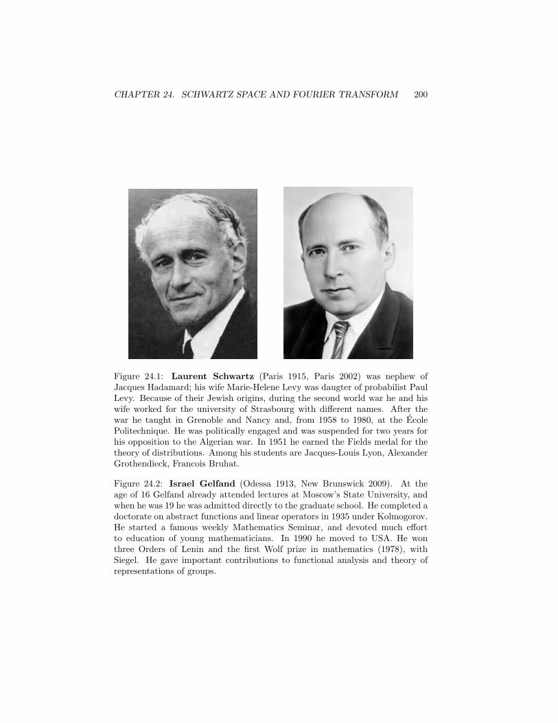
CHAPTER 24. SCHWARTZ SPACE AND FOURIER TRANSFORM 200
Figure 24.1: Laurent Schwartz (Paris 1915, Paris 2002) was nephew ofJacques Hadamard; his wife Marie-Helene Levy was daugter of probabilist PaulLevy. Because of their Jewish origins, during the second world war he and hiswife worked for the university of Strasbourg with different names. After thewar he taught in Grenoble and Nancy and, from 1958 to 1980, at the EcolePolitechnique. He was politically engaged and was suspended for two years forhis opposition to the Algerian war. In 1951 he earned the Fields medal for thetheory of distributions. Among his students are Jacques-Louis Lyon, AlexanderGrothendieck, Francois Bruhat.
Figure 24.2: Israel Gelfand (Odessa 1913, New Brunswick 2009). At theage of 16 Gelfand already attended lectures at Moscow’s State University, andwhen he was 19 he was admitted directly to the graduate school. He completed adoctorate on abstract functions and linear operators in 1935 under Kolmogorov.He started a famous weekly Mathematics Seminar, and devoted much effortto education of young mathematicians. In 1990 he moved to USA. He wonthree Orders of Lenin and the first Wolf prize in mathematics (1978), withSiegel. He gave important contributions to functional analysis and theory ofrepresentations of groups.
CHAPTER 24. SCHWARTZ SPACE AND FOURIER TRANSFORM 201
24.2 The Schwartz space
Definition 24.2.1. The Schwartz space S (R) of rapidly decreasing functionsis the set of C∞ functions φ : R → C such that for all m,n ∈ N:
∥φ∥m,n = supx∈R
|xm(Dnφ)(x)| <∞ (24.1)
Hereafter D = d/dx. The functions and their derivatives fall off at infinity morequickly than the inverse of any polynomial. By the obvious properties:1) ∥λφ∥m,n = |λ| ∥φ∥m,n,2) ∥φ1 + φ2∥m,n ≤ ∥φ1∥m,n + ∥φ2∥m,n,the Schwartz space is a linear space, and ∥ · ∥m,n is a family of seminorms for it(actually each one is a norm on S ).
S (R) ⊂ C (R) (Banach space of bounded continuous functions with sup norm):
∥φ∥∞ = supx∈R
|φ(x)| = ∥φ∥0,0 <∞
S (R) ⊂ L 1(R). The following trick is used frequenly:
∥φ∥1 =
∫Rdx |φ(x)| ≤ sup
x|(1 + x2)φ(x)|
∫R
dx
1 + x2≤ (∥φ∥0,0 + ∥φ∥2,0)π
S (R) ⊂ L p(R). Use the inequality:
∥φ∥pp =
∫Rdx|φ|p =
∫Rdx|φ|p−1 |φ| ≤ ∥φ∥p−1
∞ ∥φ∥1.
The space contains the functions e−12x
2
xn and the Hermite functions:
hn(x) =1√
2nn!√πe−
12x
2
Hn(x). (24.2)
24.2.1 Seminorms and convergence
Definition 24.2.2. A sequence of functions φr converges to φ in S (R) if:
∥φr − φ∥m,n → 0, ∀m,n.
Convergence in S (R) is very restrictive, as this example illustrates: the
sequence φr(x) = 12r e
−(rx)2 is uniformly convergent to zero (∥φr∥0,0 → 0),
but it does not converge for all seminorms: ∥φr∥0,1 = supx |xr e−(rx)2 | =
supy |ye−y2 | = 1/√2e = 0.
Definition 24.2.3. A sequence φr in S (R) is a Cauchy sequence if it is Cauchyfor every seminorm, i.e.
∀ϵ, m, n ∃Nϵ,m,n such that ∥φr − φs∥m,n < ϵ ∀r, s > Nϵ,m,n.
Bruning, Mathematical Methods in Physics, Birkhauser (2003).
CHAPTER 24. SCHWARTZ SPACE AND FOURIER TRANSFORM 202
Theorem 24.2.4. S (R) is complete in the seminorm topology3 (every Cauchysequence is seminorm-convergent).
Proof. If φr is a Cauchy sequence in S (R) then, for all (m,n), the sequencesxmDnφr are Cauchy sequences in the sup−norm and converge to functionsψm,n ∈ C (R) (which is complete in the sup-norm). In particular φr → ψ0,0. Ifwe show that ψm,n(x) = xm(Dnψ0,0)(x) for all x, it follows that ∥ψ0,0∥m,n =supx |ψm,n(x)| < ∞ and therefore ψ0,0 ∈ S (R) and φr → ψ0,0 also in theseminorm topology.
Consider the identity (xmDkφr)(x) = (xmDkφr)(0)+∫ x
0D(ymDkφr)(y)dy.
Convergence in r is uniform, so we may take the limit r → ∞ also in theintegral: ψm,k(x) = ψm,k(0) +
∫ x
0[mψm−1,k(y) + ψm,k+1(y)]dy. Therefore ψm,k
is differentiable for all m, k and
Dψm,k = mψm−1,k + ψm,k+1.
For m = 0: Dψ0,k = ψ0,k+1, i.e. ψ0,k = Dkψ0,0; this also implies that ψ0,0
can be differentiated any number of times resulting in continuous functions thatdecay to zero at infinity. The previous identity gives the following one:
ψm,k+1 − xmψ0,k+1 = D(ψm,k − xmψ0,k)−m(ψm−1,k − xm−1ψ0,k)
Iteration provides ψm,k+1−xmψ0,k+1 as a linear combination of powers of deriva-tives of the simpler functions ψm,0 − xmψ0,0. To show that ψm,k = xmDkψ0,0
it is then sufficient to prove that ψm,0 = xmψ0,0. This is done here:
|ψm,0 − xmψ0,0| ≤ |ψm,0 − xmφr|+ |xmφr − xmψ0,0|≤ sup
x|ψm,0 − xmφr|+ |x|m sup
x|φr − ψ0,0|
≤ ϵ(1 + |x|m), ∀r > Nϵ
where both ϵ and Nϵ are independent of x (uniform convergence).
Exercise 24.2.5.1) Show that ∥ · ∥0,2 is a norm in S (R).2) Show that convergence in S (R) implies L2 convergence.
Proposition 24.2.6. The linear operators (Q0φ)(x) = xφ(x) and (P0φ)(x) =−iφ′(x) on S (R) are continuous in the seminorm topology.
Proof. The identity Dn(xφ) = xDnφ + nDn−1φ implies ∥Q0φ∥m,n = supx|xmDn(xφ)| ≤ ∥φ∥m+1,n+n∥φ∥m,n−1. Similarly: ∥P0φ∥m,n = supx |xmDnφ′| =∥φ∥m,n+1. If φk → 0 then Q0φk → 0 and P0φk → 0.
Exercise 24.2.7. Show that the operator P0 is invertible. What is the domainof the inverse operator?
3such spaces are named Frechet spaces.
CHAPTER 24. SCHWARTZ SPACE AND FOURIER TRANSFORM 203
24.3 The Fourier Transform in S (R)A main motivation to introduce the Schwartz space is the special behaviour ofthe Fourier transform in this space.
Definition 24.3.1. The Fourier transform and antitransform of a function inS (R) are:
(Fφ)(k) =
∫R
dx√2πe−ikxφ(x) (24.3)
(F−1φ)(k) =
∫R
dx√2πeikxφ(x) (24.4)
The notation anticipates that FF−1 = 1: this will be a main result toprove. The transforms are related by (F−1φ)(k) = (Fφ)(−k) and are welldefined, as S (R) ⊂ L 1(R).
Theorem 24.3.2. The Fourier transform F and antitransform F−1 are con-tinuous maps of S (R) on itself.
Proof. We must show that all seminorms of (Fφ)(k) are finite:
kmdn
dkn(Fφ)(k) =
∫R
dx√2π
(−ix)nφ(x)(−i ddx
)m
e−ikx
= . . . =
∫R
dx√2πe−ikx
(id
dx
)m
[(−ix)nφ(x)]
Multiply and divide by 1 + x2 and note that Dm(xnφ) =∑m
p=0 cpxn−pDm−pφ
(cp = 0 if n− p < 0, and the precise values of cp have no relevance here). Then:
∥Fφ∥m,n ≤√π/2
m∑p=0
|cp|(∥φ∥n−p,m−p + ∥φ∥n−p+2,m−p) <∞
Then Fφ ∈ S (R). The Fourier transform is also continuous (a sequenceseminorm-convergent to zero is mapped to a sequence seminorm-convergent tozero). The same conclusions hold for F−1.
Lemma 24.3.3. If φ is in S (R) and Eϵ(x) = e−ϵx2
(ϵ ≥ 0), then Eϵφ→ φ inS (R) as ϵ→ 0.
Proof. The product Eϵφ is C∞ and belongs to S (R) and
∥Eϵφ− φ∥m,n = supx
|xmDn(Eϵφ− φ)(x)|
In the right-hand side, each derivative of Eϵ produces a factor ϵ. Then, the termwith no derivatives of Eϵ is to be considered in the limit:
limϵ→0
∥Eϵφ− φ∥m,n = limϵ→0
supx(1− e−ϵx2
)|xmφ(n)(x)|
For x = 0 the function is zero, for x = 0: (1 − e−ϵx2
) ≤ 2ϵx2. The limit iszero.
CHAPTER 24. SCHWARTZ SPACE AND FOURIER TRANSFORM 204
Theorem 24.3.4 (Inversion theorem).
φ(x) =
∫R
dk√2πeikx(Fφ)(k) (24.5)
Proof. The double integral is meaningful because Fφ ∈ S (R):
I(x) =
∫R
dk√2πeikx
∫R
dy√2πe−ikyφ(y)
To circumvent the difficulty that the two integrals cannot be exchanged, letus replace (Fφ)(k) with e−ϵk2
(Fφ)(k) ∈ S (R). The new function EϵFφconverges to Fφ as ϵ→ 0 point-wise and in the seminorm topology. Since F−1
is continuous:
F−1(EϵFφ)− φ → F−1Fφ− φ in S .
We must show that the first difference vanishes. Let’s evaluate
Iϵ(x) =F−1(EϵFφ) =
∫R
dk√2πeikx−ϵk2
∫R
dy√2πe−ikyφ(y)
=
∫Rdy φ(y)
∫R
dk
2πe−ϵk2+ik(x−y) =
∫Rdy φ(y)
1√4ϵπ
e−(x−y)2/4ϵ
The function φ multiplies the Heat kernel, whose integral is one. Then:
Iϵ(x)− φ(x) =
∫Rdy [φ(x+ y)− φ(x)]
e−y2/4ϵ
√4ϵπ
=
∫Rdy φ′(ξy) y
e−y2/4ϵ
√4ϵπ
where Lagrange’s theorem was used, and ξy is a point between x and x+ y.
|Iϵ(x)− φ(x)| ≤ supξ
|φ′(ξ)|∫Rdy |y|e
−y2/4ϵ
√4ϵπ
= 2
√ϵ
π∥φ∥0,1
As ϵ→ 0 the limit is zero, for all x.
Corollary 24.3.5. (F 2φ)(x) = φ(−x); F 3 = F−1, F 4 = 1.
Proof. (F 2φ)(x) = (F−1Fφ)(−x) = φ(−x); (F 3φ)(x) = (F 2Fφ)(x) =(Fφ)(−x).
Proposition 24.3.6. The Hermite functions (24.2) are eigenfunctions of theFourier transform:
(Fhn)(k) = (−i)nhn(k) (24.6)
Proof. The Fourier transform is evaluated on the generating function of Hermitepolynomials H(t, x) = e−t2+2tx, multiplied by e−x2/2:∫R
dx√2πe−
12x
2
e−t2+2txe−ikx = et2−2ikt
∫R
dy√2πe−
y2
2 −iky =
∞∑n=0
(it)n
n!Hn(−k)e−
k2
2
CHAPTER 24. SCHWARTZ SPACE AND FOURIER TRANSFORM 205
The change y = x−2t is done in the first integral. By comparing the same powers
of tn in e−x2
2 −t2+2tx =∑∞
n=0tn
n! e− x2
2 Hn(x), and using Hn(−x) = (−1)nHn(x),one obtains the desired result:∫ ∞
−∞
dx√2πe−
x2
2 Hn(x)e−ikx = (−i)ne− k2
2 Hn(k) (24.7)
Proposition 24.3.7. In the inner product of L2(R):
(φ|Fψ) = (F−1φ|ψ), ∀φ, ψ ∈ S (R) (24.8)
(Fψ|Fφ) = (ψ|φ), ∥Fψ∥2 = ∥ψ∥2 (24.9)
Proof. ∫Rdkφ(k)(Fψ)(k) =
∫Rdkφ(k)
∫R
dx√2πe−ikxψ(x)
=
∫Rdxψ(x)
∫R
dk√2πφ(k)e−ikx =
∫Rdxψ(x)(F−1φ)(k)
The other relations follow.
Example 24.3.8 (Fourier transform of xne−a2x2
).∫R
dx√2π
xne−a2x2
e−ikx = in∂n
∂kn
∫R
dx√2πe−a2x2−ikx =
in
a√2
∂n
∂kne−
k2
4a2
Rodrigues’ formula (11.20) is used to evaluate the derivatives, and the resultcontains the Hermite polynomial of degree n:∫
R
dx√2π
xne−a2x2
e−ikx =1
(2ia)n1
a√2e−k2
4a2Hn
(k
2a
)(24.10)
The “unitarity” (24.9) of the Fourier transform gives the integral identity:∫Rdx e−(a2+b2)x2
xn+p =2in−p
(2a)n+1(2b)p+1
∫Rdke−k2 a2+b2
4a2b2 Hn
(k
2a
)Hp
(k
2b
)Note that n and p must have the same parity (or the result is zero). The lefthand side is evaluated by the change x2 = t and gives a Gamma function4.
Exercise 24.3.9. Evaluate the Fourier transform of e−x2
(x+ a)n.
Proposition 24.3.10.
Q0F = F P0, P0F = −F Q0, (24.11)
Proof. Integrate by parts. Boundary terms cancel because φ is of rapid decrease:
(Q0Fφ)(k) = k(Fφ)(k) =
∫R
dx√2πφ(x) i
d
dxe−ikx
=
∫R
dx√2πe−ikx(−i) d
dxφ(x) = (F P0φ)(k)
The other equality is proven similarly.
Exercise 24.3.11. Show that the operators P 20 + Q2
0 and F commute.
4A useful source of tabulated integrals is Gradshteyn - Ryzhik, Tables of Integrals, Productsand Series, Academic Press.
CHAPTER 24. SCHWARTZ SPACE AND FOURIER TRANSFORM 206
24.4 Convolution product
Definition 24.4.1. The convolution product of two functions in S (R) is
(ψ ∗ φ)(x) =∫Rdy ψ(x− y) φ(y) (24.12)
Exercise 24.4.2. Prove that the convolution product is commutative.
Theorem 24.4.3. ψ ∗φ ∈ S (R) if ψ and φ are in S (R). The map ψ → ψ ∗φis linear and continuous,
F (ψ ∗ φ) =√2π (Fψ)(Fφ) , (Fψ) ∗ (Fφ) =
√2πF (ψφ) (24.13)
The convolution product is commutative, associative and distributive.
Proof. The convolution of two functions in S is in S :
|xmDn(ψ∗φ)(x)| ≤∫Rdy|xmDn
zψ(z)||φ(y)| ≤m∑ℓ=0
cℓ
∫dy|zm−ℓDn
zψ(z)||yℓφ(y)|
where z = x− y and cℓ are binomial coefficients,
≤∑ℓ
cℓ∥ψ∥m−ℓ,n
∫dy|yℓφ(y)|1 + y2
1 + y2≤ π
∑ℓ
cℓ∥ψ∥m−ℓ,n(∥φ∥ℓ,0 + ∥φ∥ℓ+2,0)
The Fourier transform:
F (ψ ∗ φ)(k) =∫
dx√2πe−ikx
∫dyψ(x− y)ϕ(y)
=
∫dyϕ(y)e−iky
∫dx√2πe−ik(x−y)ψ(x− y) =
√2π(Fφ)(k) (Fψ)(k)
The other relation follows: replace ψ,φ by Fψ, Fφ; then F (Fψ ∗ Fφ)(x) =√2πψ(−x)φ(−x). Apply F−1 = F 3 and obtain Fψ ∗ Fφ =
√2πF (ψφ).
The identity F [(φ1∗φ2)∗φ3] =√2πF (φ1∗φ2)F (φ3) = 2πF (φ1)F (φ2)F (φ3)
shows that the product is associative.
A special case is the autocorrelation function. Define the involution φ⋆(x) =φ(−x). Then:
(φ ∗ φ⋆)(x) =
∫Rdy φ(x+ y)φ(y) (24.14)
It is: (φ ∗ φ⋆)(0) =∫R dy|φ(y)|
2, F (φ ∗ φ⋆)(x) =√2π|Fφ(x)|2.
24.4.1 The Heat Equation
In one space dimension the heat (or diffusion) equation is(1
D
∂
∂t− ∂2
∂x2
)u(x, t) = 0 (24.15)
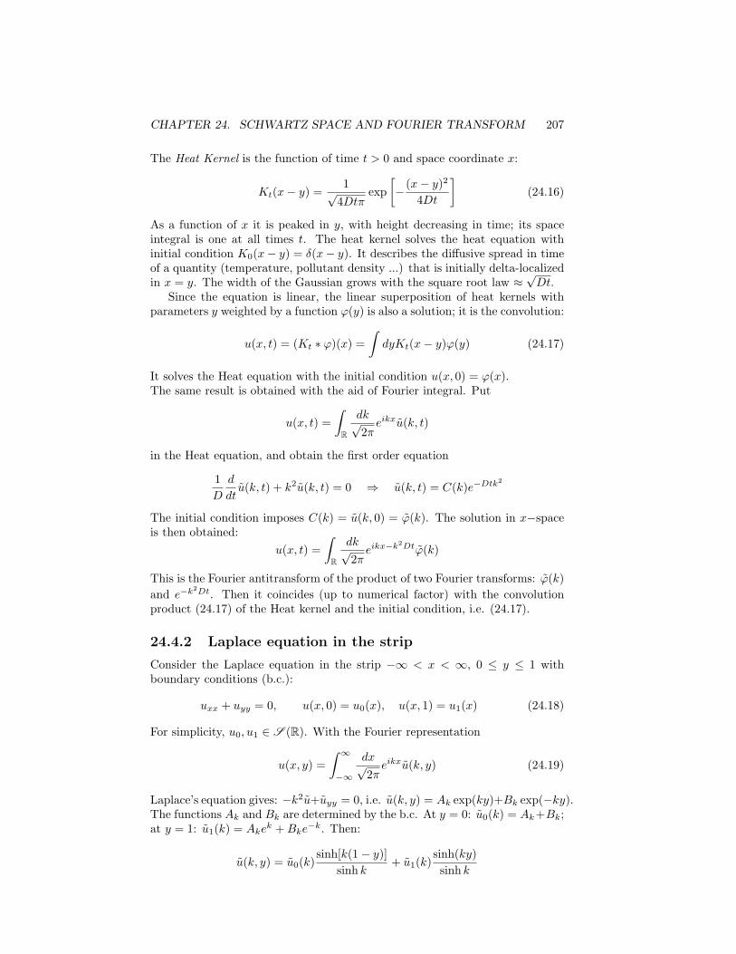
CHAPTER 24. SCHWARTZ SPACE AND FOURIER TRANSFORM 207
The Heat Kernel is the function of time t > 0 and space coordinate x:
Kt(x− y) =1√4Dtπ
exp
[− (x− y)2
4Dt
](24.16)
As a function of x it is peaked in y, with height decreasing in time; its spaceintegral is one at all times t. The heat kernel solves the heat equation withinitial condition K0(x− y) = δ(x− y). It describes the diffusive spread in timeof a quantity (temperature, pollutant density ...) that is initially delta-localizedin x = y. The width of the Gaussian grows with the square root law ≈
√Dt.
Since the equation is linear, the linear superposition of heat kernels withparameters y weighted by a function φ(y) is also a solution; it is the convolution:
u(x, t) = (Kt ∗ φ)(x) =∫dyKt(x− y)φ(y) (24.17)
It solves the Heat equation with the initial condition u(x, 0) = φ(x).The same result is obtained with the aid of Fourier integral. Put
u(x, t) =
∫R
dk√2πeikxu(k, t)
in the Heat equation, and obtain the first order equation
1
D
d
dtu(k, t) + k2u(k, t) = 0 ⇒ u(k, t) = C(k)e−Dtk2
The initial condition imposes C(k) = u(k, 0) = φ(k). The solution in x−spaceis then obtained:
u(x, t) =
∫R
dk√2πeikx−k2Dtφ(k)
This is the Fourier antitransform of the product of two Fourier transforms: φ(k)
and e−k2Dt. Then it coincides (up to numerical factor) with the convolutionproduct (24.17) of the Heat kernel and the initial condition, i.e. (24.17).
24.4.2 Laplace equation in the strip
Consider the Laplace equation in the strip −∞ < x < ∞, 0 ≤ y ≤ 1 withboundary conditions (b.c.):
uxx + uyy = 0, u(x, 0) = u0(x), u(x, 1) = u1(x) (24.18)
For simplicity, u0, u1 ∈ S (R). With the Fourier representation
u(x, y) =
∫ ∞
−∞
dx√2πeikxu(k, y) (24.19)
Laplace’s equation gives: −k2u+uyy = 0, i.e. u(k, y) = Ak exp(ky)+Bk exp(−ky).The functions Ak and Bk are determined by the b.c. At y = 0: u0(k) = Ak+Bk;at y = 1: u1(k) = Ake
k +Bke−k. Then:
u(k, y) = u0(k)sinh[k(1− y)]
sinh k+ u1(k)
sinh(ky)
sinh k
CHAPTER 24. SCHWARTZ SPACE AND FOURIER TRANSFORM 208
To evaluate u(x, y) by (24.19) we exploit the properties of the convolution.Let’s identify u as products of Fourier transforms: u(k, y) = u0(k)S1−y(k) +
u1(k)Sy(k) where Sy(k) is evaluated with the Residue theorem (see ex.14.3.19):
Sy(k) =
∫ ∞
−∞
dk√2πeikx
sinh(ky)
sinh k=
√π
2
sin(πy)
cosh(πx) + cos(πy)
The Fourier transform (24.19) becomes the sum of two convolutions, and thesolution of the Laplace equation in the strip is obtained:
u(x, y) =1√2π
[(Sy ∗ u1)(x) + (S1−y ∗ u0)(x)]
=1
2
∫ ∞
−∞dx′
[sin(πy)u1(x
′)
cosh[π(x− x′)] + cos(πy)+
sin(πy)u0(x′)
cosh[π(x− x′)]− cos(πy)
].
Chapter 25
TEMPEREDDISTRIBUTIONS
... Depuis l’introduction par Dirac de la fameuse fonction δ(x), qui seraitnulle partout sauf pour x = 0 et serait infinie pour x = 0 de telle sort que∫ +∞−∞ dx δ(x) = +1, les formules du calcul symbolique sont devenues plus inac-ceptables pour la rigueur des mathematiciens. Ecrire que la fonction d’Heavisideθ(x) egale a 0 pour x < 0 et a 1 pour x ≥ 0 a pour derive la fonction de Diracδ(x) dont la definition meme est mathematiquement contradictoire, et parlerde derivees δ′(x), δ′′(x) ... de cette fonction denuee d’existence reelle, c’estdepasser les limites qui nous sont permises ... (L. Schwartz, “Theorie des Dis-tributions”, Hermann & C. Paris, 1950)
25.1 Introduction
The linear functionals on Schwartz’s space provide a generalization of ordinaryfunctions that is very useful in the theory of differential equations and in thespectral theory of operators.A linear continuous functional is a linear map f : S (R) → C such that for anyseminorm-convergent sequence φk → 0, the sequence of complex numbers fφk
converges to zero.A sufficient condition for continuity is boundedness with respect to a seminorm(or a finite sum of seminorms): there are a constant Cf and a seminorm suchthat:
|fφ| ≤ Cf∥φ∥k,m ∀φ ∈ S (R).Definition 25.1.1. The space of continuous functionals on S (R) is S ′(R), thespace of tempered distributions.
It is a linear space with the linear operations (f +λg)φ = fφ+λ (gφ). If f andg are sequentially continuous, so are their linear combinations1.The regular distributions are the integral functionals
fφ =
∫Rdxf(x)φ(x)
1A nice and instructive presentation is: I. Richards and H. Youn, Theory of distributions:a non-technical introduction, Cambridge University Press (1990).
209
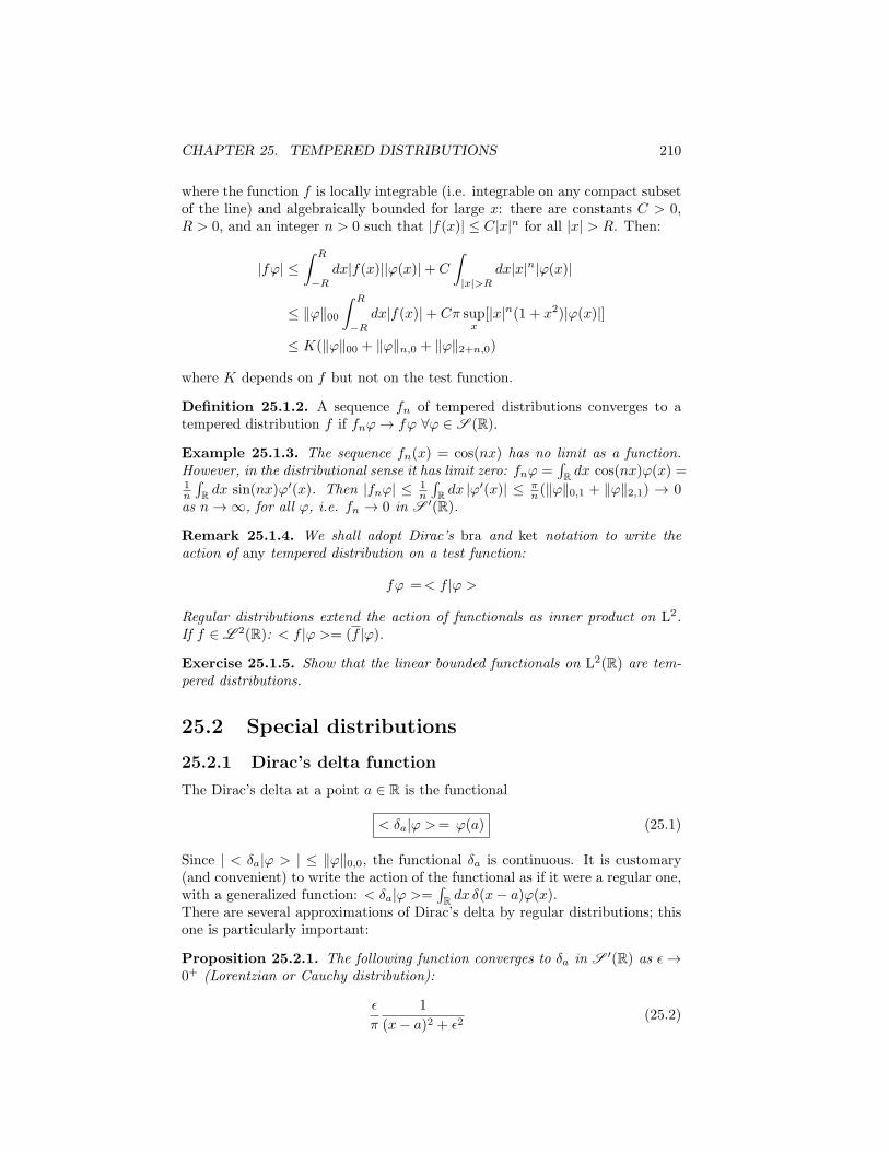
CHAPTER 25. TEMPERED DISTRIBUTIONS 210
where the function f is locally integrable (i.e. integrable on any compact subsetof the line) and algebraically bounded for large x: there are constants C > 0,R > 0, and an integer n > 0 such that |f(x)| ≤ C|x|n for all |x| > R. Then:
|fφ| ≤∫ R
−R
dx|f(x)||φ(x)|+ C
∫|x|>R
dx|x|n|φ(x)|
≤ ∥φ∥00∫ R
−R
dx|f(x)|+ Cπ supx[|x|n(1 + x2)|φ(x)|]
≤ K(∥φ∥00 + ∥φ∥n,0 + ∥φ∥2+n,0)
where K depends on f but not on the test function.
Definition 25.1.2. A sequence fn of tempered distributions converges to atempered distribution f if fnφ→ fφ ∀φ ∈ S (R).
Example 25.1.3. The sequence fn(x) = cos(nx) has no limit as a function.However, in the distributional sense it has limit zero: fnφ =
∫R dx cos(nx)φ(x) =
1n
∫R dx sin(nx)φ′(x). Then |fnφ| ≤ 1
n
∫R dx |φ
′(x)| ≤ πn (∥φ∥0,1 + ∥φ∥2,1) → 0
as n→ ∞, for all φ, i.e. fn → 0 in S ′(R).
Remark 25.1.4. We shall adopt Dirac’s bra and ket notation to write theaction of any tempered distribution on a test function:
fφ =< f |φ >
Regular distributions extend the action of functionals as inner product on L2.If f ∈ L 2(R): < f |φ >= (f |φ).
Exercise 25.1.5. Show that the linear bounded functionals on L2(R) are tem-pered distributions.
25.2 Special distributions
25.2.1 Dirac’s delta function
The Dirac’s delta at a point a ∈ R is the functional
< δa|φ >= φ(a) (25.1)
Since | < δa|φ > | ≤ ∥φ∥0,0, the functional δa is continuous. It is customary(and convenient) to write the action of the functional as if it were a regular one,with a generalized function: < δa|φ >=
∫R dx δ(x− a)φ(x).
There are several approximations of Dirac’s delta by regular distributions; thisone is particularly important:
Proposition 25.2.1. The following function converges to δa in S ′(R) as ϵ→0+ (Lorentzian or Cauchy distribution):
ϵ
π
1
(x− a)2 + ϵ2(25.2)
CHAPTER 25. TEMPERED DISTRIBUTIONS 211
Proof. For any ϵ the function is integrable and normalized. Let’s show that forany test function φ, the action on φ converges to φ(a) as ϵ→ 0. This amountsto the vanishing of the integral∫
Rdx
ϵ
π
φ(x)− φ(a)
(x− a)2 + ϵ2=
∫ ∞
0
dxϵ
π
φ(a+ x) + φ(a− x)− 2φ(a)
x2 + ϵ2
The integral is split into∫ 1
0+∫∞1
. In the first integral Lagrange’s formula isused for the differences: |φ(a± x)− φ(a)| = |φ′(ξ±)|x (where ξ± is some pointin the interval). Then the modulus of the first integral is majorized by
2ϵ
πsups
|φ′(s)|∫ 1
0
x dx
x2 + ϵ2=ϵ
π∥φ∥0,1 log[(1/ϵ)2 + 1]
The modulus of the second integral is majorized by:
4ϵ
πsups
|φ(s)|∫ ∞
1
dx
x2 + ϵ2=
4
π∥φ∥00
[π
2− arctan
1
ϵ
]Both terms vanish for ϵ→ 0+.
Exercise 25.2.2. Try another proof with the replacement x = a + ϵ tan θ fol-lowed by an integration by parts.
The following regular distributions also converge to δa in S ′(R) as ϵ → 0+
(proofs are simple and left as exercise)
1√πϵe−
1ϵ (x−a)2 ,
1
2ϵχ[a−ϵ,a+ϵ](x) (25.3)
Exercise 25.2.3. Show that the sequences converge to δ0:
2
πϵ2
√ϵ2 − x2 θ(ϵ2 − x2),
sin(nx)
πx.
(Hint for the second case: the function [φ(x) − φ(0)χ[−1,1](x)]/x is in L 1(R)for φ ∈ S (R). Use the Riemann-Lebesgue theorem 26.1.3).
25.2.2 Heaviside’s theta function
Consider the functional θa, a ∈ R,
< θa|φ >=
∫ ∞
a
dxφ(x) (25.4)
It is a regular distribution, with function θ(x− a) = χ[a,∞)(x).
CHAPTER 25. TEMPERED DISTRIBUTIONS 212
Exercise 25.2.4.Prove the distributional limits (n→ ∞)2
1) χ[0,n] → θ(x),
2) fn(x) =
0 x < 0
xn x = [0, 1]
x = 1 x > 1
→ θ(x− 1)
3)1
enx + 1→ θ(−x).
25.2.3 Principal value of 1x−a
The function 1x−a has a non-integrable singularity in x = a and thus it does not
yield a regular distribution. One then defines the “principal value of 1x−a” as
the functional
< P 1x−a |φ >= −
∫Rdx
φ(x)
x− a(25.5)
The principal value is:
limϵ→0+
(∫ a−ϵ
−∞dx+
∫ ∞
a+ϵ
dx
)φ(x)
x− a= lim
ϵ→0+
∫ ∞
ϵ
dxφ(a+ x)− φ(a− x)
x;
the limit ϵ → 0+ exists: use Lagrange’s formula on the interval ϵ ≤ x ≤ 1, andthe triangle inequality on x ≥ 1:∣∣∣< P 1
x−a |φ >∣∣∣ ≤ 2(1− ϵ) sup
x|φ′(x)|+
∫ ∞
1
dx(|φ(a+ x)|+ |φ(a− x)|)
≤ 2∥φ∥0,1 + 2∥φ∥L1
The L1 norm is majored by seminorms, therefore the principal part is a tempereddistribution. Note the equivalence of the expressions:
limϵ→0+
∫ ∞
ϵ
dxφ(a+ x)− φ(a− x)
x= −
∫ ∞
0
dx log x [φ′(a+ x) + φ′(a− x)]
25.2.4 The Sokhotski-Plemelj formulae
The following identities among distributions are extremely useful in the study ofGreen functions (differential equations, potential theory, linear response theory,spectral theory of operators)3:
limϵ→0+
1
x− a± iϵ= P
1
x− a∓ iπδ(x− a) (25.6)
2The function 3) with n = µkBT
and x = E−µµ
is the Fermi-Dirac distribution, which gives
the average number of identical fermions (e.g. electrons in metals) with energy E, in thermalequilibrium at temperature T and chemical potential µ > 0. The limit distribution, θ(µ−E),is the Fermi distribution. It is the state at T = 0 (ground state).
3The identities were discovered by Sokhotski in 1873, and proven rigorously about thirtyyears later by Josip Plemelj. Given a Cauchy integral on a curve (it can be open or closed)
F (z) =
∫γ
dζ
2πi
f(ζ)
ζ − z, z /∈ γ
CHAPTER 25. TEMPERED DISTRIBUTIONS 213
a is real and the limit is distributional, i.e.
limϵ→0+
∫Rdx
φ(x)
x− a± iϵ= −∫Rdx
φ(x)
x− a∓ iπ φ(a), φ ∈ S (R)
Proof. The real part is the distribution with action∫Rdx
(x− a)φ(x)
(x− a)2 + ϵ2=
∫Rdxxφ(x+ a)
x2 + ϵ2=
∫ ∞
0
dxx
x2 + ϵ2[φ(a+ x)− φ(a− x)]
= −∫ ∞
0
dx log√x2 + ϵ2[φ′(a+ x) + φ′(a− x)]
which, for ϵ→ 0, converges to −∫
φx−a (see previous section). The imaginary part
is a regular distribution that converges to the delta function:∫Rdx
∓ϵ(x− a)2 + ϵ2
φ(x) → ∓πφ(a).
Exercise 25.2.5. Prove the identity, for real x, y, and ϵ, η > 0:∫R
dx′
π2Re
[1
x′ − x+ iϵ
]Re
[1
x′ − y + iη
]=
1
π
ϵ+ η
(x− y)2 + (ϵ+ η)2(25.7)
Therefore, for x = y and in the limit ϵ+ η → 0+:∫dx′
π2
P
x′ − x
P
x′ − y= δ(x− y) (25.8)
Exercise 25.2.6 (Hilbert transform). The Hilbert transform of a functionis
(H f)(x) = −∫R
dx′
π
f(x′)
x− x′(25.9)
By means of (25.8) show that (H 2φ)(x) = −φ(x). Therefore, the solution ofthe integral equation H f = g is f = −H g.
Exercise 25.2.7. Show that this is a tempered distribution:
< P1
x2|φ >= lim
ϵ→0+
[ ∫ −ϵ
−∞dx
φ(x)− φ(0)
x2+
∫ ∞
ϵ
dxφ(x)− φ(0)
x2
](25.10)
Can you suggest a generalization to define P (1/xn)?
Example: zeros of large-n Hermite polynomialsLet x1 . . . xn be the (real) zeros of the Hermite polynomial Hn(x): we wish toevaluate their density when n is large. The polynomial solves the differentialequation H ′′
n(x) − 2xH ′n(x) + 2nHn(x) = 0, which becomes Weber’s equation
and the Holder condition |f(ζ)−f(ζ0)| ≤ A|ζ− ζ0|α (A, α > 0) for all ζ, ζ0 ∈ γ, the identitiesestablish the limits F±(ζ0) as z approaches a point ζ0 ∈ γ different than endpoints, from theleft or the right sides of γ.The identities are frequently used in theoretical physics with the path γ given by the real axis.
CHAPTER 25. TEMPERED DISTRIBUTIONS 214
for the Hermite function (the equation for the harmonic oscillator in quantummechanics):
−h′′n(x) + (x2 − 2n− 1)hn(x) = 0, hn(x) =1√
n! 2n√πe−
12x
2
Hn(x).
If x2 > 2n + 1, hn(x) and h′′n(x) have the same sign, and vanish at infinity.Therefore, as |x| decreases from ∞, |hn(x)| increases. For a zero to occur thecurvature h′′n must change sign, and the function may start to point to the realaxis. In conclusion, the zeros of Hn(x) are confined in the interval x2 < 2n+1.
Rescale the zeros xi = si√2n, (i = 1 . . . n); if a limit distribution exists the
rescaled zeros si are described by a density ρ(s) = limn→∞1n
∑ni=1 δ(s − si)
with expected support σ = [−1, 1]. To evaluate the density let’s introduce theuseful function Fn(z), with its limit function:
Fn(z) =1
n
n∑i=1
1
z − si→ F (z) =
∫σ
dsρ(s)
z − sz /∈ σ
For large |z| it behaves as 1/z. By the Sokhotski-Plemelj identity:
ρ(s) =1
πImF (s− iϵ) (25.11)
The limit function F (z) is obtained from Fn(z) by noting that
H ′n(x)
Hn(x)=
n∑i=1
1
x−√2n si
=
√n
2Fn
(x√2n
)A derivative in x and the equation H ′′
n(x) − 2xH ′n(x) + 2nHn(x) = 0 give the
Riccati equation1
nF ′n(z) + F 2
n(z)− 4zFn(z) + 4 = 0
In the large-n limit the derivative is neglected: F 2(z) − 4zF (z) + 4 = 0. Thesolution with correct large z asymptotics is: F (z) = 2z − 2
√z2 − 1. Eq.(25.11)
gives the semicircle law:
ρ(s) =
2π
√1− s2 if |s| < 1
0 if |s| > 1(25.12)
It is a remarkable fact that the semicircle law also describes the distribution ofeigenvalues of Hermitian matrices with random matrix elements, in the large nlimit.
Example: Semicircle law of GUE random matricesThe study of random matrices in physics was started by Wigner and Dysonin the Fifties as a reference model for the statistical properties of sequences ofnuclear resonances. For example, it was noticed that the energy separations sof resonances normalized by an average value, obey the same statistical lawsP (s) ≈ sβe−ks2 of random matrices (k is a constant, β is 1 for real symmetricmatrices, 2 for complex Hermitian matrices and 4 for quaternionic self-dual).
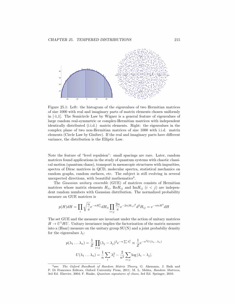
CHAPTER 25. TEMPERED DISTRIBUTIONS 215
-40 -20 0 20 40
10
20
30
40
-0.6 -0.4 -0.2 0.2 0.4 0.6
-0.4
-0.2
0.2
0.4
Figure 25.1: Left: the histogram of the eigenvalues of two Hermitian matricesof size 1000 with real and imaginary parts of matrix elements chosen uniformlyin [-1,1]. The Semicircle Law by Wigner is a general feature of eigenvalues oflarge random real-symmetric or complex-Hermitian matrices with independentidentically distributed (i.i.d.) matrix elements. Right: the eigenvalues in thecomplex plane of two non-Hermitian matrices of size 1000 with i.i.d. matrixelements (Circle Law by Ginibre). If the real and imaginary parts have differentvariance, the distribution is the Elliptic Law.
Note the feature of “level repulsion”: small spacings are rare. Later, randommatrices found applications in the study of quantum systems with chaotic classi-cal motion (quantum chaos), transport in mesoscopic structures with impurities,spectra of Dirac matrices in QCD, molecular spectra, statistical mechanics onrandom graphs, random surfaces, etc. The subject is still evolving in severalunexpected directions, with beautiful mathematics4.
The Gaussian unitary ensemble (GUE) of matrices consists of Hermitianmatrices whose matrix elements Hii, ReHij and ImHij (i < j) are indepen-dent random numbers with Gaussian distribution. The normalized probabilitymeasure on GUE matrices is
p(H)dH =∏i
√n
πe−nH2
iidHii
∏i<j
2n
πe−2n|Hij |2d2Hij = e−ntrH2
dH
The set GUE and the measure are invariant under the action of unitary matricesH → U†HU . Unitary invariance implies the factorization of the matrix measureinto a (Haar) measure on the unitary group SU(N) and a joint probabiliy densityfor the eigenvalues λi:
p(λ1 . . . λn) =1
Z
∏i<j
(λj − λj)2e−n
∑λ2i ≡ 1
Ze−n2U(λ1...λn)
U(λ1 . . . λn) =1
n
∑i
λ2i −2
n2
∑i<j
log |λi − λj |.
4see: The Oxford Handbook of Random Matrix Theory, G. Akemann, J. Baik andP. Di Francesco Editors, Oxford University Press, 2011; M. L. Mehta, Random Matrices,3rd Ed. Elsevier, 2004; F. Haake, Quantum signatures of chaos, 3rd Ed. Springer, 2010.
CHAPTER 25. TEMPERED DISTRIBUTIONS 216
with normalization constant Z =∫dλ1 . . . dλn exp(−n2U). For GUE the joint
probability density vanishes quadratically for degenerate eigenvalues (degener-ate eigenvalues are rare, with level repulsion exponent β = 2)5.For large n, the largest contribution to the probability density comes from theset of eigenvalues that minimize the “potential energy” U . This configurationdetermines the statistical properties of eigenvalues of GUE matrices for n→ ∞.It has the interpretation of minimal energy state of a bidimensional gas of ncharged particles (log potential) in a harmonic potential. The minimum solves
∂U
∂λi= 0 i.e. λi =
2
n
∑j =i
1
λi − λj→ xi =
∑j =i
1
xi − xj, xi =
√n
2λi
The solution is found by a nice trick (Stieltjes): define the polynomial p(x) =(x − x1) · · · (x − xn). By eq.(9.2) the n conditions for minimum become: xi =p′′(xi)/p
′(xi) i.e. the polynomial p′′(x)−xp′(x) must be zero at x = x1, . . . , xn.Since it is of degree n, it is proportional to p(x) itself. Then p′′(x) − xp′(x) +np(x) = 0, with solution p(x) = cnHn(x
√2). Therefore, for n → ∞ the eigen-
values of a random GUE matrix (with probability one) have a semicircle distri-bution with radius determined by the variance of the Gaussian (in this case theradius in 1
2
√n).
25.3 Distributional calculus
Important operations such as conjugation, derivative, Fourier transform, maybe extended simply and naturally from well behaved functions (such as testfunctions or functions associated to regular distributions) to distributions (gen-eralized functions, which may be as awkward as a delta function). The procedurereproduces the steps of this first example.
Complex conjugation has a natural definition if the distribution is regular:if f is the regular distribution < f |φ >=
∫dx f(x)φ(x), its complex conjugate
is the distribution f∗ with action < f∗|φ >=∫dx f(x)φ(x) = < f |φ >. As the
last equality does not depend on f being a regular distribution, it provides theextension:
Definition 25.3.1. The complex conjugate of a distribution f is the distribu-tion
< f∗|φ >= < f |φ > (25.13)
Example 25.3.2. The Dirac’s delta is real: δ∗a = δa.
5A simple argument for level repulsion. Let x, y be the real eigenvalues of the 2× 2 GUEmatrix (β = 2): (
a b− icb+ ic d
), |x− y| =
√(a− d)2 + 4b2 + 4c2
To have x = y we need that the random numbers a− d, b and c are zero simultaneously: thisis very unlikely. For random real symmeric matrices (GOE) it is c = 0 and level repulsion isweaker (β = 1).
CHAPTER 25. TEMPERED DISTRIBUTIONS 217
Along the same line one defines the multiplication of a tempered distributionby a C∞ function g that is algebraically bounded with all its derivatives6. It isthe tempered distribution
< gf |φ >=< f |g φ > (25.14)
25.3.1 Derivative
Consider a regular distribution with a function f ∈ C 1(R) such that f ′ stilldefines a regular distribution. Then:
< f ′|φ >=∫ ∞
−∞dx f ′φ = −
∫ ∞
−∞dx fφ′ = − < f |φ′ > .
This evaluation suggests the definition of the derivative of any distribution:
Definition 25.3.3. The derivative of a distribution f is the distribution f ′ withaction
< f ′|φ >= − < f |φ′ > (25.15)
As derivation is a continuous operator on S (R), the derivative of tem-pered distributions gives tempered distributions, and is linear and continuouson S ′(R). One can evaluate as many derivatives of a distribution as wanted.
Example 25.3.4. Derivative of Heaviside’s functional θa.By definition: < θ′a|φ >= − < θa|φ′ >= −
∫∞aφ′(x)dx = φ(a). Therefore:
θ′a = δa, or
d
dxθ(x− a) = δ(x− a)
Example 25.3.5. Derivative of δa. By definition: < δ′a|φ >= −φ′(a).
Exercise 25.3.6. Show that: ddx |x| = signx, < d
dxδa|φ >= − dda < δa|φ >.
Example 25.3.7. The derivative of F (x) = θ(x2−m2), m > 0, is by definition:
< F ′|φ >= −∫ −m
−∞ dxφ′(x)−∫∞mdxφ′(x) = −φ(−m)+φ(m) =< δm−δ−m|φ >.
As an identity among generalized functions one writes:
d
dxθ(x2 −m2) = δ(x−m)− δ(x+m).
Remark 25.3.8. In ordinary calculus one would write: ddxθ(x
2−m2) = 2x δ(x2−m2), leading to the conclusion
δ(x2 −m2) =1
2x[δ(x−m)− δ(x+m)] =
1
2m[δ(x−m) + δ(x+m)]
This can be generalized; the evaluation of the derivative of θ(f(x)), where f is asmooth real function with isolated zeros x1, . . . , xn, leads to the useful formula:
δ(f(x)) =n∑
k=1
δ(x− xk)
|f ′(xk)|(25.16)
6g(x) = cos(ex) is bounded and smooth, but g′(x) is unbounded
CHAPTER 25. TEMPERED DISTRIBUTIONS 218
We state but not prove the following characterization of tempered distribu-tions:
Theorem 25.3.9. Every tempered distribution is the distributional derivativeof finite order of a continuous algebraically bounded function: f ∈ S ′(R) ⇔there is a continuous function ξ such that |ξ(x)| ≤ C(1 + |x|n) for some C andn, and k ≥ 0 such that
< f |φ >=< ξ(k)|φ >= (−1)k∫ ∞
−∞dx ξ(x)φ(k)(x).
25.3.2 Fourier transform
To extend the Fourier transform to distributions, start from regular functionals.Suppose that both f and Ff are functions that produce regular distributions(for example f is in S ). Then:
< Ff |φ >=∫Rdx(Ff)(x)φ(x) =
∫Rdxφ(x)
∫R
dk√2πe−ikxf(k)
=
∫Rdk f(k)
∫R
dx√2πe−ikxφ(x) =< f |Fφ >
The extension to all distributions is:
Definition 25.3.10. The Fourier transform of a tempered distribution f is thedistribution Ff with action
< Ff |φ >=< f |Fφ > (25.17)
Proposition 25.3.11. The Fourier transform F : S ′(R) → S ′(R) is invert-ible (FF−1f = f) and continuous.
Proof. Continuity and the inversion property are exported from the same prop-erties in S (R): < F−1Ff |φ >=< Ff |F−1φ >=< f |FF−1φ >=< f |φ >.Since the Fourier transform is linear, it is enough to check continuity in the ori-gin: let fn → 0 in S ′(R) then < Ffn|φ >=< fn|Fφ >→ 0 i.e. Ffn → 0.
Example 25.3.12. Fourier transform of δa.
< F δa|φ >=< δa|Fφ >= (Fφ)(a) =
∫Rdxe−iax
√2π
φ(x).
The Fourier transform of Dirac’s delta is the regular distribution with function:
(F δa)(x) =e−iax
√2π
(25.18)
In particular: 1 =√2πF δ0 (=
√2πF−1δ0).
The same result is obtained by exploiting the continuity of the Fourier transform,acting on a regular approximation of δa. For example:
uϵ(x) =1
π
ϵ
(x− a)2 + ϵ2, (Fuϵ)(x) =
1√2πe−ϵ|x|−ixa (25.19)
CHAPTER 25. TEMPERED DISTRIBUTIONS 219
As a family of regular distributions, for ϵ → 0 the sequence uϵ converges toδa. The sequence of Fourier transforms also converges in S ′ and the limit is(25.18).
Example 25.3.13. The following approximation of the delta function is useful:
limN→∞
sin(Nx)
πx= δ0 (25.20)
A simple proof based on continuity of the Fourier transform: since χ[−N,N ] → 1
in S ′(R), then Fχ[−N,N ] →√2πδ0.
Example 25.3.14.
Fxn = in√2π δ
(n)0 (25.21)
< Fxn|φ >=< 1|xnFφ >= (−i)n < 1|Fφ(n) >. Since 1 =√2πF−1δ0, it is:
< Fxn|φ >= (−i)n√2π < δ0|φ(n) >= in
√2π < δ
(n)0 |φ >
Example 25.3.15. Fourier transform of P 1x−a .
< FP 1x−a |φ >= −
∫dx
x− a
∫R
dk√2πe−ikxφ(k) =
∫R
dk√2πφ(k)e−ika−
∫R
dx
xe−ikx.
The Principal-value integral is:
−∫R
dx
xe−ikx = −i
∫Rdx
sin(kx)
x= −iπ sign(k).
Then we obtain the regular distribution
(FP 1x−a )(k) = −i
√π
2sign(k)e−ika (25.22)
Example 25.3.16. Fourier transform of θa.
< Fθa|φ >=< θa|Fφ >=
∫ ∞
a
dx
∫R
dy√2πe−ixyφ(y)
Since integrals cannot be exchanged, introduce a convergence factor and considerthe Fourier transform of the distributions θa,ϵ(x) = e−ϵxθa(x) (ϵ > 0). Asθa,ϵ → θa and the Fourier transform is continuous in S ′, it is
< Fθa|φ >= limϵ→0+
∫ ∞
a
dx e−ϵx
∫R
dy√2πe−ixyφ(y)
=
∫Rdy φ(y)
∫ ∞
a
dx√2πe−ixy−ϵx =
∫Rdy
1
i√2π
e−iay
y − iϵφ(y)
In the last line it is understood that the limit ϵ → 0+ is taken. The limit canbe done after the action on a test function is evaluated (this is the meaning ofconvergence of distributions). We obtain Fθa as a limit of regular distributions:
(Fθa)(x) =1
i√2π
e−iax
x− iϵ. (25.23)
CHAPTER 25. TEMPERED DISTRIBUTIONS 220
Inversion gives a useful representation of Heaviside’s function:
θ(x− a) =
∫ ∞
−∞
dk
2πi
eik(x−a)
k − iϵ= −
∫ ∞
−∞
dk
2πi
e−ik(x−a)
k + iϵ(25.24)
Example 25.3.17. Fourier transform of the sign-function.A convergence factor is introduced, and the limit ϵ→ 0+ is understood.
< F sign|φ >=< sign|Fφ >=
∫Rdx sign(x)e−ϵ|x|
∫R
dy√2πe−ixyφ(y)
=
∫Rdy φ(y)
∫R
dx√2πe−ixy−ϵ|x|sign(x) =
∫Rdy
1√2π
−2ik
y2 + ϵ2φ(y)
Therefore we have the sequence in ϵ of regular distributions:
(F sign)(x) =1√2π
−2ix
x2 + ϵ2= −i
√2
πRe
1
x+ iϵ= −i
√2
πP1
x(25.25)
The Plemelj-Sokhotski formula was used in the last equality.
Exercise 25.3.18. Evaluate the Fourier transform of the following generalizedfunctions: 1) (x− a); 2) log |x|; 3) exp(−iωx), ω ∈ R.
Exercise 25.3.19. What is the Plemelj-Sokhotski identity after Fourier trans-form?
25.4 Fourier series and distributions
Definition 25.4.1. A tempered distribution f is periodic with period τ if< f |Uτφ >=< f |φ >, where (Uτφ)(x) = φ(x− τ).
We state a generalization of Fourier series (but omit the proof), that is welldefined as a distribution although it may not converge as an ordinary function:
Theorem 25.4.2. f is a τ−periodic tempered distribution if and only if thereare constants cn with |cn| < C(1 + |n|k) for some k, such that
f =∑n∈Z
cn exp
(i2πn
τx
), i.e. < f |φ >=
∑n∈Z
cn
∫Rdxφ(x) exp
(i2πn
τx
)or, equivalently:
Ff =√2π∑n∈Z
cnδ2πn/τ , i.e. < Ff |φ >=√2π∑n∈Z
cnφ
(2πn
τ
)Example 25.4.3. Consider the periodic distribution ∆x =
∑n∈Z δx+nτ , with
action < ∆x|φ >=∑
n φ(x + nτ). The series is well defined because φ isin S (R), and defines a periodic function g(x) with period τ . Then, g can beexpanded in Fourier series: g(x) =
∑n gne
i(2π/τ)nx.
CHAPTER 25. TEMPERED DISTRIBUTIONS 221
25.5 The Kramers - Kronig relations
The theory of linear response evaluates the effects produced on a system bythe coupling to a weak time-dependent field δφ(t), in the linear approximation.The physical requirement of causality, i.e. the effect on the system may onlydepend on the field’s values at earlier times, has general implications that aredescribed by the Kramers - Kronig relations for the response function.
Let g(t) be the value at time t of a measurable quantity of the system inpresence of the perturbation, and g0(t) be the value of the same quantity inabsence of the perturbation. In the linear approximation, the variation δg(t) =g(t) − g0(t) is linearly related to the external perturbation through a responsefunction R(t, t′) that only depends on the variables of the unperturbed system:
δg(t) =
∫ t
−∞R(t, t′) δφ(t′)dt′
The integral involves the history of the system at times less than t because ofthe physical requirement of causality.If the properties of the unperturbed system are time-independent (as in ther-mal equilibrium), the response function depends on t − t′ and the integral is aconvolution:
δg(t) =
∫ ∞
−∞θ(t− t′)R(t− t′) δφ(t′)dt′ (25.26)
Hereafter we consider this very common situation.In frequency space the convolution (25.26) becomes the product of the Fouriertransforms7, and the linear response takes the simple form of a direct propor-tionality between response and driving field at the same frequency:
δg(ω) = χ(ω)δφ(ω) (25.27)
Notable examples are: J = σE, M = χH, D = ϵE (where each quantitydepends on ω, with possible further dependence on wave-vector). The responsefunction χ(ω) is the generalized susceptibility. It is evaluated with the aid of theFourier representation (25.24) of the theta function:
χ(ω) =
∫Rd(t− t′) eiω(t−t′) θ(t− t′)R(t− t′)
=
∫Rds eiωs
∫R
dω′
2πi
eiω′s
ω′ − iϵR(s)
=
∫R
dω′
2πi
1
ω′ − iϵ
∫Rds ei(ω
′+ω)sR(s)
=
∫R
dω′
2πi
R(ω′)
ω′ − ω − iϵ
This representation shows that χ(ω), as a function of complex frequency, isanalytic on Im ω ≥ 0. This is a consequence of causality and, in turn, it impliesthe Kramers - Kronig relations. They were obtained independently in 1926 and1927, and relate the real and imaginary parts of the response in ω space:
7In physics it is customary to define the Fourier transform of a function of time as f(ω) =∫R dtf(t)eiωt, with inverse f(t) =
∫R
dω2π
f(ω)e−iωt. In this section we use this convention.
CHAPTER 25. TEMPERED DISTRIBUTIONS 222
Proposition 25.5.1. Suppose that χ(ω) → 0 if |ω| → ∞; for real ω it is:
Reχ(ω) = −−∫ ∞
−∞
dω′
π
Imχ(ω′)
ω − ω′ , Imχ(ω) = −∫ ∞
−∞
dω′
π
Reχ(ω′)
ω − ω′ (25.28)
Proof. Consider the integral ∫Rdω′ χ(ω′)
ω − ω′ + iϵ
The path of integration is closed with a semicircle in the upper half plane, whereχ is analytic. The integral vanishes, and the Plemelj-Sokhotski formula is used:
0 =
∫Rdω′ χ(ω′)
ω − ω′ + iϵ= −∫Rdω′ χ(ω
′)
ω − ω′ − iπχ(ω)
Separation of real and imaginary parts gives the relations.
25.6 The Gel’fand triplet
We’ll prove that the Hermite functions are a complete orthonormal system inL2(R), therefore the Schwartz space S (R) is dense in L2(R), i.e. any square-integrable function is the limit of a L2norm-convergent sequence of rapidly de-creasing functions.By Riesz’s theorem L2(R) is self-dual, i.e. each function f can be viewed asa linear sequentially continuous functional on L2(R) and thus as a tempereddistribution (up to conjugation):
| < f |φ > | = |(f |φ)| ≤ ∥f∥2∥φ∥2 ≤ const.∥f∥2 supx(1 + x2)|φ(x)|
for all test functions. Therefore we have the relation (Gel’fand triplet):
S (R) ⊂ L2(R) ⊂ S ′(R) (25.29)
The structure is useful for extending operators on domain including S (R) toS ′(R), and to give meaning to expansions of L2 functions in terms of generalizedfunctions.
25.7 Linear operators on distributions
Suppose that an operator A : S (R) → S (R) is linear and continuous (conver-gent sequences are mapped to convergent sequences, in the seminorm topology).If f is a tempered distribution, the functional φ→< f |Aφ > is a tempered dis-tribution. Therefore, the operator A induces an “adjoint” operator on tempereddistributions: A′ : S ′(R) → S ′(R)
< A′f |φ >=< f |Aφ >, f ∈ S ′(R), φ ∈ S (R) (25.30)
Being A densely defined in L2(R), the adjoint A† exists: (A†f |φ) = (f |Aφ),∀f ∈ D(A†), ∀φ ∈ S (R). By viewing A†f and f as elements of the dual space
CHAPTER 25. TEMPERED DISTRIBUTIONS 223
L2(R)∗, and thus as distributions, we rewrite it as < (A†f)∗|φ >=< f∗|Aφ >,i.e. < (A†f∗)∗|φ >=< f |Aφ >. Therefore, for distributions that are functionsf ∈ D(A†) it is
A′f = (A†f∗)∗ (25.31)
With this rule, A′ is an extension of A† to S ′.
25.7.1 Generalized eigenvectors
The eigenvalue equation A′f = λf has solution in S ′ if
∃ fλ such that < fλ|Aφ >= λ < fλ|φ > ∀φ ∈ S (R). (25.32)
fλ is a ”generalized eigenvector”.
Example 25.7.1. The operator (Q0φ)(x) = xφ(x) leaves S invariant and iscontinuous; the corresponding operator Q′
0 acts on distributions as multiplicationby the algebraically bounded function x. The eigenvalue equation Q′
0fλ = λfλ,i.e. < fλ|Q0φ >= λ < fλ|φ > ∀φ has solution for any real λ: fλ = δλ.Note the “completeness” property with respect to the inner product of L2:
(φ1|φ2) =
∫Rdλ< δλ|φ1 > < δλ|φ2 > .
Example 25.7.2. The operator P0φ = −iφ′ leaves S invariant and is continu-ous. The operator P ′
0 on distributions is < P ′0f |φ >=< f |− iφ′ >= i < f ′|φ >,
i.e. P ′0f = if ′. The eigenvalue equation P ′
0eλ = λeλ is solved by the ordinaryfunctions eλ(x) = e−iλx/
√2π, λ ∈ R (Im λ = 0 gives exponentially divergent
functions, which do not give regular distributions). The normalization is suchthat < eλ|φ >= (Fφ)(λ), which implies the completeness property:
(φ1|φ2) =
∫Rdλ< eλ|φ1 > < eλ|φ2 > .
25.7.2 Green functions
Let A : S → S be a linear continuous operator. If it exists, the Green functionof the operator A is the distribution that solves the equation
A′Gx = δx, x ∈ R
i.e. < Gx|Aφ >= φ(x), for all test functions. Written in terms of a generalizedfunction it is
∫dx′Gx(x
′)(Aφ)(x′) = φ(x).
Proposition 25.7.3. Consider the inhomogeneous equation Aφ = ψ, with as-signed ψ ∈ S (R). If Gx is the Green function of A, a particular solution is:
φ(x) =< Gx|ψ >=
∫dy Gx(y)ψ(y)
Proof. φ(x) =< δx|φ >=< A′Gx|φ >=< Gx|Aφ >=< Gx|ψ >.
CHAPTER 25. TEMPERED DISTRIBUTIONS 224
Example 25.7.4. The Green function for P0 = −iD solves iDGy = δy. Asolution is Gy = −iθy i.e. Gy(x) = −iθ(x− y).The equation P0φ = ψ is solved by φ(y) = −i
∫dx θ(x−y)ψ(x) = −i
∫∞ydxψ(x),
up to a constant (a solution of the homogeneous equation).
Example 25.7.5 (Forced oscillator).
(Lφ)(t) = ψ(t), L =d2
dt2+Ω2
The general solution is the sum of a solution of the homogeneous equation,φ0(t) = A cos(Ωt) + B sin(Ωt), with a particular solution. The Green functionof L solves L′Gt = δt, where t has to be regarded as an index and
< L′f |φ >=< f |Lφ >=< f |φ′′ +Ω2φ >=< D′′f +Ω2f |φ > .
Therefore the equation for the Green function is (D2 +Ω2)Gt = δt i.e.
d2
ds2Gt(s) + Ω2Gt(s) = δ(s− t)
The equation is solved in Fourier space. It is customary to name ω the variableconjugated to time s:
Gt(s) =
∫R
dω√2πgt(ω)e
iωs, (−ω2 +Ω2)gt(ω) =1√2πe−iωt
Because of the zeros ±Ω the general solution contains a principal value prescrip-tion and delta terms supported on the zeros:
gt(ω) =1√2πe−iωt
[P
Ω2 − ω2+ αδ(ω − Ω) + βδ(ω +Ω)
],
α and β are arbitrary constants. Then
Gt(s) = −P∫R
dω
2π
e−iω(t−s)
ω2 − Ω2+
α
2πe−iΩ(t−s) +
β
2πeiΩ(t−s)
A family of particular solutions φ(t) =∫RGt(s)ψ(s)ds is obtained, where the
delta functions produce terms that solve the homogeneous equation. There isfreedom in the determination of the Green function.By the Sokhotski-Plemelj formulae, the principal part and the delta functionsmay combine to give small imaginary parts to the poles ±Ω. The choice wherethe poles are in the half-plane Im ω < 0 (i.e. the poles are ±Ω− iϵ) defines theretarded Green function:
GR(t− s) =
∫R
dω
4πΩe−iω(t−s)
[1
ω +Ω+ iϵ− 1
ω − Ω+ iϵ
]= θ(t− s)
1
Ωsin[Ω(t− s)] (25.33)
The particular solution
φ(t) = (GR ∗ ψ)(t) = 1
Ω
∫ t
−∞ds sin[Ω(t− s)]ψ(s)
has the property of causality: its value at time t only depends on the forcing fieldψ at earlier times. This makes the retarded Green function of special importancein physics.
CHAPTER 25. TEMPERED DISTRIBUTIONS 225
25.7.3 Wave equation with source
The wave equation with source ρ is xφ(x) = −ρ(x), where x = (x, ct), andx = ∇2 − 1
c2 ∂2t is the wave operator. The Green function (or “fundamental
solution”) of the wave operator is the distribution that solves
xG(x, x′) = −δ4(x− x′) (25.34)
Then, φ(x) = φ0(x) +∫d4x′G(x, x′)ρ(x′) where φ0 solves the homogeneous
equation, xφ0 = 0.As we shall see, the Green function is not unique. Its determination can bedictated by physics. For example causality requires that the field φ at time tcannot depend on values of the source ρ at later times t′ > t (actually, becauseof the finite wave speed c, the effect is further delayed). Being the equation(25.34) translation-invariant, we’ll solve it by the Fourier expansion
G(x, x′) =
∫d4k
(2π)4eik·(x−x′)G(k)
where k = (k, ω/c), k · x = k · x − ωt. In Fourier space eq.(25.34) is algebraic:
−(k · k)G(k) = −1 i.e. (|k|2 − (ω/c)2)G(k, ω) = 1. Therefore
G(x, x′) =
∫d3k
(2π)3eik·(x−x′)
∫ ∞
−∞
dω
2πce−iω(t−t′) (−c2)
ω2 − |k|2c2
A general feature occurs: the integral is singular with poles at ω = ±|k|c. Thisis no problem: we are dealing with distributions, and small epsilons may beintroduced to shift poles off the real axis. As this can be done in different ways,there are different Green functions.Causality determines one choice of the signs. If t′ > t the integration path closesin the upper half-plane (this ensures exponential decay on the semicircle); if werequire that G(x, x′) = 0 for t′ > t, no poles must be encircled, i.e. the two polesare in the lower half plane. This choice defines the retarded Green function:
GR(x, x′) =
∫d3k
(2π)3eik·(x−x′)
∫ ∞
−∞
dω
2πe−iω(t−t′) (−c)
(ω + iϵ)2 − |k|2c2
= θ(t− t′)
∫d3k
(2π)3eik·(x−x′) −c
2|k|c
[e−i|k|c(t−t′) − ei|k|c(t−t′)
]= θ(t− t′)
∫ ∞
0
k2dk
(2π)2−1
2k
[e−ikc(t−t′) − eikc(t−t′)
] ∫ π
−π
sin θ dθeik|x−x′| cos θ
= θ(t− t′)
∫ ∞
0
dk
8π2
[e−ikc(t−t′) − eikc(t−t′)
] [eik|x−x′| − e−ik|x−x′|
]A change k → −k gives the sum of two delta functions, one of which is identicallyzero, and a factor 2π. Then:
GR(x, x′) = θ(t− t′)1
4π|x− x′|δ(|x− x′| − c(t− t′))
The Green function has support on the spherical surface centred in x′ withradius c(t− t′) > 0, increasing with t. The causal field with source ρ(x′, t′) is a
CHAPTER 25. TEMPERED DISTRIBUTIONS 226
continuous superposition of such spherical waves being emitted at every pointof the source:
φ(x, t) =
∫d3x′
∫ t
−∞dt′
1
4π|x− x′|δ(|x− x′| − c(t− t′))ρ(x′, t′)
=
∫d3x′
ρ(x′, t− |x− x′|/c)4πc |x− x′|
(25.35)
Chapter 26
FOURIER TRANSFORMII
The Fourier transform F and antitransform F−1 were studied in detail in S (R)and extended to the dual space. The same properties generalize to S (Rn) andthe dual, with
(Fu)(q) =
∫Rn
dnx
(2π)n/2e−iq·xu(x) (26.1)
(F−1u)(q) =
∫Rn
dnx
(2π)n/2eiq·xu(x) (26.2)
It is of great interest to investigate the properties of F as operators on the spacesLp(Rn). Here we restrict to one dimension (n = 1). Most of the propertiescontinue to hold in higher dimension.
26.1 Fourier transform in L1(R)By the inequality |Fu(k)| ≤
∫R dx |u(x)| the Fourier transform is well defined
on the whole space L 1(R), and |Fu(k)| ≤ 1√2π
∥u∥1 for all k. Therefore F is a
linear operator from L1(R) to L∞(R), and
∥Fu∥∞ ≤ 1√2π
∥u∥1
The operator is continuous: if un → u in L1(R) then Fun → Fu uniformly:
|(Fun)(k)− (Fu)(k)| ≤∫R
dx√2π
|un(x)− u(x)| = 1√2π
∥un − u∥1
i.e. Fun → Fu in L∞(R).
Exercise 26.1.1. What is the condition for an integrable real function to havea real Fourier transform?
Example 26.1.2. The Fourier transform of a characteristic function
(Fχ[a,b])(k) =
∫ b
a
dx√2πe−ik x =
√2
π
sin[ b−a2 k]
ke−i b+a
2 k
227
CHAPTER 26. FOURIER TRANSFORM II 228
is a continuous bounded function, i.e. ∈ C (R), and vanishes for |k| → ∞.
The same properties hold true for ladder functions σ, which are finite linearcombinations of χ functions, and are a dense subset of L1(R). This anticipatesthe fundamental theorem:
Theorem 26.1.3 (Riemann - Lebesgue). If f ∈ L 1(R) then Ff is bounded,continuous, and
lim|k|→∞
|(Ff)(k)| = 0 (26.3)
Proof. Integrable functions can be approximated by ladder functions. If σn is asequence of ladder functions convergent to f in L1, then Fσn → Ff uniformly.Since Fσn are continuous, also Ff is continuous1.∀ϵ there is a ladder function σ such that ∥f − σ∥1 < ϵ. Since |Fσ| vanishes atinfinity, there is R such that for |k| > R it is |(Fσ)(k)| < ϵ. Then, for |k| > Rit is:
|(Ff)(k)| ≤ |F (f − σ)(k)|+ |(Fσ)(k)| ≤ 1√2π
∥u− σ∥1 + |(Fσ)(k)| < ϵ
up to finite constants.
We make some statements without proof:
Proposition 26.1.4. Let f, g ∈ L 1(R):1) the convolution product
(f ∗ g)(x) =∫Rdy f(x− y)g(y) (26.4)
is a function in L 1(R) and ∥f ∗ g∥1 ≤ ∥f∥1∥g∥1. As the Fourier transformexists for all terms, it can be proven that
F (f ∗ g) =√2π(Ff)(Fg) (26.5)
2) since the Fourier transforms are bounded, the following integrals exist andare equal (Fubini’s theorem applies):∫
Rdk(Ff)(k)g(k) =
∫Rdkf(k)(F−1g)(k) (26.6)
3) with a proof quite similar to that given for S , it can be proven that for func-tions in L 1(R) such that their transform remains L 1, the inversion theoremholds: FF−1 = 1.
1If fn is a sequence of continuous functions that converges to f uniformly, then f iscontinuous. Proof: for any x it is |f(x) − f(y)| ≤ |f(x) − fn(x)| + |f(y) − fn(y)| + |fn(x) −fn(y)| ≤ 3ϵ for n large enough and |y − x| < δ.
CHAPTER 26. FOURIER TRANSFORM II 229
26.2 Fourier transform in L2(R)Hermite functions belong to S (R) ⊂ L2(R). The following theorem has variousinteresting implications:
Theorem 26.2.1. The Hermite functions hm are an orthonormal and completeset in L2(R).
Proof. From the generating function of Hermite polynomials (11.17) one obtainsthat of Hermite functions:
h(x, z) =∞∑
m=0
zm√m!hm(x) =
14√πe−
12 (x
2−2√2zx+z2)
The series converges point-wise and also in L2 norm. Suppose that there is afunction f in L2 such that (hm|f) = 0 for all m. This implies that (h|f) = 0 forall z. For z = −ik/2
√2, up to irrelevant factors, it is
0 =
∫R
dx√2π
e−12x
2−ixkf(x) = (Fg)(k), g(x) = e−12x
2
f(x)
The function g belongs to L1(R) (Schwartz inequality) and its Fourier transformis zero. Then g ∈ KerF ; but the inversion theorem in L1 implies Ker F = 0,then g = 0 i.e. f = 0.
The Schwartz space is dense in L2. Since the Fourier transform is isomet-ric on S (R) (∥Fφ∥2 = ∥φ∥2), it may be extended to a unitary operator Fon L2(R). The explicit construction exploits the property of hn to be eigen-states of F and to form an orthonormal complete set. From the expansionf =
∑n(hn|f)hn we obtain by linearity and continuity of F :
Theorem 26.2.2 (Fourier-Plancherel operator). The Fourier transform Fextends uniquely to a unitary operator F : L2(R) → L2(R):
F f =∞∑
n=0
(−i)n (hn|f)hn (26.7)
The inverse transform F−1 extends uniquely to the adjoint F †.
Remark 26.2.3. The Hermite functions are the eigenfunctions of the numberoperator N = 1
2 (P2 + Q2 − 1): Nhn = nhn. The operator is the generator in
L2(R) of the one-parameter unitary group
U(θ) = e−iθN =∞∑
n=0
e−inθ(hn| · )hn
with domain D(N) = f :∑∞
n=0 n2|(hn|f)|2 < ∞. The group describes the
2π-periodic evolution in time θ of the quantum oscillator (in phase space, meanvalues of position and momentum make a circular motion). Both the generatorN and U(θ) leave S (R) invariant. It is U(π2 ) = F , U(−π
2 ) = F−1 = F †. U(π)is the parity operator.
CHAPTER 26. FOURIER TRANSFORM II 230
Another way to evaluate the Fourier transform of a function f ∈ L 2 is toconsider the functions χ[−R,R]f ∈ L 1(R). On such functions F = F and, since
F is continuous:
(F f)(k) = l.i.m.R→∞
∫ R
−R
dx√2πe−ikxf(x)
where l.i.m. is ”limit in the mean”, i.e. in L2 topology.
26.2.1 Completeness of the Fourier basis
The Fourier transform of a function in S (R) can be written as
(Fφ)(k) =
∫Rdxuk(x)φ(x) =< uk|φ >, uk(x) =
eikx√2π, k ∈ Z
where < uk| > is not the inner product but the action of a regular distribution.By the inversion theorem for the Fourier transform in S it is:
φ(x) =
∫Rdk < uk|φ > uk(x) (26.8)
Since Schwartz’s space is dense in L2, the relation shows the completeness ofthe continuous system of functions uk. They are the eigenfunctions of thederivative operator on distributions, which extends the self-adjoint unboundedoperator P .
Proposition 26.2.4 (Vladimirov2).
φ ∈ S (R) ⇐⇒∞∑
n=0
n2k|φn|2 <∞ ∀ k ∈ N (26.9)
where φn = (hn|φ) are the coefficients of the expansion in the Hermite basis.
Similarly one proves the theorem: f ∈ S ′(R) if and only if there are apositive constants C, p such that | < f |un > | ≤ C(1 + n)p, for all n ∈ N.
2V. Vladimirov, Le distribuzioni nella fisica matematica, Mir (1981).
Chapter 27
THE LAPLACETRANSFORM
27.1 The Laplace integral
The Fourier transform exists for functions that belong to L 1(R): this is veryrestrictive in applications, for it leaves out several important functions. How-ever, if one replaces a non-integrable function f(x) by e−cxf(x) (Re c > 0),integrability may be achieved for large x; at the same time, to avoid problemsat the other end of integration, one requires f(x) = 0 for x < 0. Then, if∫ ∞
0
dx e−cx |f(x)| <∞
for a suitable value c, one can evaluate the Fourier integral of√2πe−cxf(x):∫∞
0dx e−ikxe−cxf(x). By setting z = c + ik, the Fourier integral defines the
Laplace transform of f :
(L f)(z) =
∫ ∞
0
dxf(x)e−zx (27.1)
The complex function is well defined for Re z ≥ c, where c is some real numberthat depends on f , and is bounded:
|(L f)(z)| ≤∫ ∞
0
dx e−xRez|f(x)| ≤ (L |f |)(c)
Proposition 27.1.1.lim
Re z→∞|(L f)(z)| = 0
Proof. The sequence |e−zxf(x)| has limit 0 for any x as |z| → ∞. Since it equalse−x(Rez−c)e−cx|f(x)|, it is definitely bounded by e−cx|f(x)| ∈ L1(R+). By thedominated convergence theorem, the limit can be taken in the integral sign.
Lemma 27.1.2. If |(L f)(z)| <∞ for Rez > c+ ϵ then |(L xnf)(z)| <∞ forRez > c+ ϵ.
231
CHAPTER 27. THE LAPLACE TRANSFORM 232
Proof.∣∣∫∞
0dx e−zxxnf(x)
∣∣ ≤ supx≥0[xne−x(Rez−c−ϵ)]
∫∞0dx e−(c+ϵ)x|f(x)| <
∞
Theorem 27.1.3. (L f)(z) is holomorphic in the half-plane Re z > c and
d
dz(L f)(z) = −(L xf)(z) (27.2)
Proof. Let’s show that the limit h→ 0 exists:∣∣∣∣ (L f)(z + h)− (L f)(z)
h+ (L xf)(z)
∣∣∣∣ = ∣∣∣∣∫ ∞
0
dx e−xzf(x)
[e−hx − 1
h+ x
]∣∣∣∣≤∫ ∞
0
dx e−xRez|f(x)|∣∣∣∣e−hx − 1
h+ x
∣∣∣∣ ≤ |h|2
∫ ∞
0
dx e−xzx2|f(x)| → 0
where the following inequality is used∣∣∣∣e−hx − 1
h+ x
∣∣∣∣ = ∣∣∣∣∫ x
0
dy(e−hy − 1)
∣∣∣∣ ≤ ∫ x
0
dy|e−yh − 1| ≤ 12 |h|x
2
The last step is proven here: let y > 0, h = h1+ ih2, then: |e−yh−1| = |e−yh1 −eiyh2 | = [(e−yh1 − 1)2 + 4e−yh1 sin2( 12yh2)]
1/2 ≤√(yh1)2 + (yh2)2 = y|h| by
means of Lagrange’s formula and the bound | sinx/x| ≤ 1.
27.2 Properties
These properties are proven without difficulty:
L (af + bg) = aL f + bL g (linearity) (27.3)
(L f)(z) = (L f)(z) (27.4)
(L f ′)(z) = −f(0) + z(L f)(z) (27.5)
(L f ′′)(z) = −f ′(0)− zf(0) + z2(L f)(z) (27.6)
(L xf)(z) = −(L f)′(z) (27.7)
(L e−axf)(z) = (L f)(z + a). (27.8)
Some simple Laplace transforms:
(L [eαx])(z) =1
z − α, Re z > Re α (27.9)
(L [sinωx])(z) =ω
z2 + ω2, Re z > 0 (27.10)
(L [cosωx])(z) =z
z2 + ω2, Re z > 0 (27.11)
Example 27.2.1.
(L [xa−1])(z) =
∫ ∞
0
dx e−zxxa−1 =Γ(a)
za, Re a > 0, Re z > 0 (27.12)
Logs and powers can be included by replacing a by a+ ϵ, and expanding in ϵ:
xa−1+ϵ = xa−1[1 + ϵ log x+ 12ϵ
2(log x)2 + . . . ]
Γ(a+ ϵ) = Γ(a)[1 + ϵ ψ(a) + 12ϵ
2ψ2(a) + . . . ]
CHAPTER 27. THE LAPLACE TRANSFORM 233
where ψ(z) is the digamma function etc. By equating equal powers of ϵ oneobtains (Re z > 0):
(L [xa−1 log x])(z) =Γ(a)
za[ψ(a)− Logz] (27.13)
(L [xa−1 log2 x])(z) =Γ(a)
za[ψ2(a)− 2ψ(a)Logz − Log2z] (27.14)
27.3 Inversion
The Laplace transform can be inverted. With the understanding that f(x) = 0for x < 0, recall the correspondence:
(F [√2πe−axf(x)])(k) = (L f)(a+ ik)
If, as a function of k, it is (L f)(a+ ik) ∈ L 1(R), the Fourier transform can beinverted: √
2πe−axf(x) =
∫ ∞
−∞
dk√2π
(L f)(a+ ik)eikx.
The formula transforms into: f(x) =∫∞−∞
dk2π e
(a+ik)x(L f)(a + ik). Put z =a+ ik, dz = idk and the inversion formula is obtained:
f(x) =
∫ a+i∞
a−i∞
dz
2πiezx(L f)(z) (27.15)
The line of integration is parallel to the imaginary axis with a > c. The func-tion (L f)(z) is analytic for Re z > c. If it is meromorphic for Rez < c, thecomputation of the integral can be done by the Residue Theorem, by closing theintegration path by a semicircle in Re z < c surrounding the poles (Bromwich’scontour).
27.3.1 Hankel’s representation of Γ
The antitransform of (L [xa−1])(z) is
xa−1 = Γ(a)
∫ c+i∞
c−i∞
dz
2πiezxz−a
where c > 0 is arbitrary. For x = 1 Hankel’s integral representation of theGamma function is obtained:
1
Γ(a)=
∫ ϵ+i∞
ϵ−i∞
dz
2πiezz−a (27.16)
The path of integration can be deformed to the loop shown in fig. 27.1. Inparticular, if a = n the singularity is a pole in the origin, the loop may bedeformed to a circle, and the Residue Theorem gives Γ(n) = (n− 1)!.
If a = n the evaluation of the loop integral gives an important identity of theGamma function. Let za = eaLogz; the loop runs along the cut of discontinuity
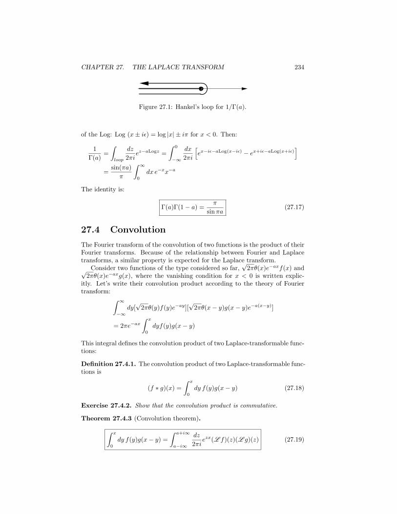
CHAPTER 27. THE LAPLACE TRANSFORM 234
Figure 27.1: Hankel’s loop for 1/Γ(a).
of the Log: Log (x± iϵ) = log |x| ± iπ for x < 0. Then:
1
Γ(a)=
∫loop
dz
2πiez−aLogz =
∫ 0
−∞
dx
2πi
[ex−iϵ−aLog(x−iϵ) − ex+iϵ−aLog(x+iϵ)
]=
sin(πa)
π
∫ ∞
0
dx e−xx−a
The identity is:
Γ(a)Γ(1− a) =π
sinπa(27.17)
27.4 Convolution
The Fourier transform of the convolution of two functions is the product of theirFourier transforms. Because of the relationship between Fourier and Laplacetransforms, a similar property is expected for the Laplace transform.
Consider two functions of the type considered so far,√2πθ(x)e−axf(x) and√
2πθ(x)e−axg(x), where the vanishing condition for x < 0 is written explic-itly. Let’s write their convolution product according to the theory of Fouriertransform: ∫ ∞
−∞dy[
√2πθ(y)f(y)e−ay][
√2πθ(x− y)g(x− y)e−a(x−y)]
= 2πe−ax
∫ x
0
dyf(y)g(x− y)
This integral defines the convolution product of two Laplace-transformable func-tions:
Definition 27.4.1. The convolution product of two Laplace-transformable func-tions is
(f ∗ g)(x) =∫ x
0
dy f(y)g(x− y) (27.18)
Exercise 27.4.2. Show that the convolution product is commutative.
Theorem 27.4.3 (Convolution theorem).
∫ x
0
dy f(y)g(x− y) =
∫ a+i∞
a−i∞
dz
2πiezx(L f)(z)(L g)(z) (27.19)
CHAPTER 27. THE LAPLACE TRANSFORM 235
Proof. We use results from the theory of Fourier transform. By the convolutiontheorem for the Fourier transform, it is
2πe−ax
∫ x
0
dyf(y)g(x− y)
=√2πF−1
(F [
√2πθ(y)f(y)e−ay]F [
√2πθ(y)g(y)e−ay]
)(x)
=
∫ ∞
−∞dk eikx(L f)(a+ ik)(L g)(a+ ik)
Therefore:∫ x
0
dyf(y)g(x− y) =
∫R
dk
2πe(a+ik)x(L f)(a+ ik)(L g)(a+ ik)
Now put z = a+ ik, dz = idk.
Example 27.4.4. The Laplace transform is useful for solving differential equa-tions. Consider the inhomogeneous equation
f ′′(t) + ω2f(t) = g(t)
with initial conditions f(0) = A and f ′(0) = B. Laplace transform yields thealgebraic equation −f ′(0)− zf(0)+ (z2 +ω2)(L f)(z) = (L g)(z), with solution
(L f)(z) =(L g)(z) +B +Az
z2 + ω2.
To obtain f one needs to invert a Laplace transform. Note that the solution canbe written as
f(t) = L −1
(L [g]
1
ωL [sinωx] +
B
ωL [sinωx] +
A
ωL [cosωx]
)=
∫ t
0
dt′sinω(t− t′)
ωg(t′) + fhom(t),
where fhom(t) = Bω sinωt + A
ω cosωt solves the homogeneous equation. Thissolution via Laplace transform exhibits the causality property: the particularsolution f at time t is determined by the values of the forcing field at timest′ < t.
27.5 Mellin transform
In analogy with the construction of the Laplace transform, the Fourier identityis formally modified to define the useful Mellin transform1. In the identity
f(x) =
∫ ∞
−∞
dk
2πe−ikx
∫ ∞
−∞dy eikyf(y) (27.20)
1for a nice introduction see: https://www.cs.purdue.edu/homes/spa/papers/chap9.ps
CHAPTER 27. THE LAPLACE TRANSFORM 236
put x = log s and y = log t: f(log s) =∫∞−∞
dk2π s
−ik∫∞0
dt tik−1f(log t); let
z = c+ ik, dz = idk: s−cf(log s) =∫ c+i∞c−i∞
dz2πis
−z∫∞0
dt tz−1t−cf(log t); rename
f(log s)s−c as f(s). The Mellin transform of a function is:
(M f)(z) =
∫ ∞
0
dxxz−1f(z) (27.21)
It exists for |(M f)(z)| ≤∫∞0dx|f(x)|xRez−1 < ∞, which means that z is
bounded in some strip of the complex plane. The inversion formula is
f(x) =
∫ c+i∞
c−i∞
dz
2πix−z(M f)(z) (27.22)
The Mellin transform of e−x is Γ(z).
Exercise 27.5.1. Prove the properties:
(Mxf)(z) = (M f)(z + 1) (27.23)
(M f ′)(z) = −(z − 1)(M f)(z − 1) (27.24)
(MxnDnf)(z) = (−1)n(z − n) . . . (z − 1)(M f)(z) (27.25)∫ ∞
0
dx|f(x)|2 =
∫ c+i∞
c−i∞
dz
2πi|M f(z)|2 (Parseval identity) (27.26)
(M fg)(z) =
∫ c+i∞
c−i∞
dz
2πi(M f)(z′)(M g)(z − z′) (27.27)
L. G. Molinari is associate professor at the Physics Department of Milan’s Uni-versita degli Studi, where he teaches mathematical methods for physics andquantum theory of many-particle systems. His main research interests are ran-dom matrix theory, Anderson localization, theory of many-particle systems,differential geometry. Since 1972 he is an active member of the AstronomicalSociety G. V. Schiaparelli, Varese, devoted to the popularization of astronomyand natural sciences.
237