Embed Size (px)
Citation preview

Mathematical Expressions of the Pharmacokinetic andPharmacodynamic Models implemented
in the PFIM software
Anne Dubois, Julie Bertrand and France Mentre
UMR738, INSERM, University Paris Diderot
Programmer: Anne Dubois
March 2011
The library of pharmacokinetic (PK) and pharmacodynamic (PD) models described in thisdocument is implemented in the PFIM software since version 3.2.1 and in PFIM Interfacesince version 3.1 (www.pfim.biostat.fr). The PK/PD libraries of PFIM are derived from thePK/PD models implemented in the Monolix software and described by Julie Bertrand andFrance Mentre in a Monolix software documentation (software.monolix.org). PFIM is a freelibrary of functions. The University Paris Diderot and INSERM are the co-owners of thislibrary of functions (version 3.2, copyright 2010).

Contents
1 Pharmacokinetic models 51.1 Compartmental models and parameters . . . . . . . . . . . . . . . . . . . . . . . 6
1.1.1 One-compartment models . . . . . . . . . . . . . . . . . . . . . . . . . . 61.1.2 Two-compartment models . . . . . . . . . . . . . . . . . . . . . . . . . . 71.1.3 Three-compartment models . . . . . . . . . . . . . . . . . . . . . . . . . 7
1.2 Models with linear elimination . . . . . . . . . . . . . . . . . . . . . . . . . . . . 91.2.1 One-compartment models . . . . . . . . . . . . . . . . . . . . . . . . . . 9
1.2.1.1 Intravenous bolus . . . . . . . . . . . . . . . . . . . . . . . . . . 91.2.1.2 Infusion . . . . . . . . . . . . . . . . . . . . . . . . . . . . . . . 91.2.1.3 First order absorption . . . . . . . . . . . . . . . . . . . . . . . 10
1.2.2 Two-compartment models . . . . . . . . . . . . . . . . . . . . . . . . . . 101.2.2.1 Intravenous bolus . . . . . . . . . . . . . . . . . . . . . . . . . . 111.2.2.2 Infusion . . . . . . . . . . . . . . . . . . . . . . . . . . . . . . . 111.2.2.3 First order absorption . . . . . . . . . . . . . . . . . . . . . . . 12
1.2.3 Three-compartment models . . . . . . . . . . . . . . . . . . . . . . . . . 131.2.3.1 Intravenous bolus . . . . . . . . . . . . . . . . . . . . . . . . . . 141.2.3.2 Infusion . . . . . . . . . . . . . . . . . . . . . . . . . . . . . . . 141.2.3.3 First order absorption . . . . . . . . . . . . . . . . . . . . . . . 16
1.3 Models with Michaelis-Menten elimination . . . . . . . . . . . . . . . . . . . . . 171.3.1 One-compartment models . . . . . . . . . . . . . . . . . . . . . . . . . . 17
1.3.1.1 Intravenous bolus . . . . . . . . . . . . . . . . . . . . . . . . . . 171.3.1.2 Infusion . . . . . . . . . . . . . . . . . . . . . . . . . . . . . . . 171.3.1.3 First order absorption . . . . . . . . . . . . . . . . . . . . . . . 18
1.3.2 Two-compartment models . . . . . . . . . . . . . . . . . . . . . . . . . . 191.3.2.1 Intravenous bolus . . . . . . . . . . . . . . . . . . . . . . . . . . 191.3.2.2 Infusion . . . . . . . . . . . . . . . . . . . . . . . . . . . . . . . 191.3.2.3 First order absorption . . . . . . . . . . . . . . . . . . . . . . . 20
1.3.3 Three-compartment models . . . . . . . . . . . . . . . . . . . . . . . . . 211.3.3.1 Intravenous bolus . . . . . . . . . . . . . . . . . . . . . . . . . . 211.3.3.2 Infusion . . . . . . . . . . . . . . . . . . . . . . . . . . . . . . . 211.3.3.3 First order absorption . . . . . . . . . . . . . . . . . . . . . . . 22
2 Pharmacodynamic models 242.1 Immediate response models . . . . . . . . . . . . . . . . . . . . . . . . . . . . . 24
2.1.1 Drug action models . . . . . . . . . . . . . . . . . . . . . . . . . . . . . . 25
3

2.1.2 Baseline/disease models . . . . . . . . . . . . . . . . . . . . . . . . . . . 262.1.3 PFIM model function examples . . . . . . . . . . . . . . . . . . . . . . . 26
2.2 Turnover response models . . . . . . . . . . . . . . . . . . . . . . . . . . . . . . 272.2.1 Models with impact on the input (Rin) . . . . . . . . . . . . . . . . . . . 272.2.2 Models with impact on the output (kout) . . . . . . . . . . . . . . . . . . 28
Appendix 29Appendix I: list of models in PK library . . . . . . . . . . . . . . . . . . . . . . . . . 29
Appendix I.1: PK models with linear elimination . . . . . . . . . . . . . . . . . 30Appendix I.1: PK models with Michaelis-Menten elimination . . . . . . . . . . . 32
Appendix II: list of models in PD library . . . . . . . . . . . . . . . . . . . . . . . . . 33Appendix II.1: Immediate response PD models for PD only . . . . . . . . . . . . 34Appendix II.2: Immediate response PD models for PK/PD . . . . . . . . . . . . 35Appendix II.3: Turnover PD models for PK/PD . . . . . . . . . . . . . . . . . . 36
4

Chapter 1
Pharmacokinetic models
The equations in the ensuing chapter describe the pharmacokinetic models implemented in thePFIM software (www.pfim.biostat.fr). The presentation of the models is organised as follows:
• First level: elimination process
– Linear
– Michaelis-Menten
• Second level: number of compartments
– One compartment
– Two compartments
– Three compartments
• Third level: route of administration
– Intravenous bolus
– Infusion
– Oral (first order absorption)
• Last level: administration profile
The equations express the concentration C (t) in the central compartment at a time t after thelast drug administration.
- Single dose: at time t after dose D given at time tD (t ≥ tD)
- Multiple doses: at time t after n doses Di (i = 1, ...n) given at time tDi(t ≥ tDn)
- Steady state (only for linear elimination): at a time t after dose D given at time tD afterrepeated administration of dose D given at interval τ (t ≥ tD)
5

1.1. COMPARTMENTAL MODELS AND PARAMETERS
NB: For infusion, the duration of infusion is Tinf for single dose and Tinfi (i = 1, ...n) formultiple doses. D is the total administered dose for single dose; Di is the total ith administereddose for multiple doses.
For multiple doses, the delay between successive doses is supposed to be constant and tobe greater than infusion duration (tDi+1
− tDi= constant and tDi+1
− tDi> Tinfi for infusion).
For steady state, the interval τ is supposed to be greater than infusion duration (τ >Tinf).
1.1 Compartmental models and parameters
In the ensuing section, the mammillary models with one, two or three compartments arepresented with the associated parameters and the different parameterisations. Six parametersare common to one, two or three compartment models:
- V or V1, the volume of distribution in the central compartment
- k, the elimination rate constant
- CL, the clearance of elimination
- Vm, the maximum elimination rate for Michaelis-Menten elimination
- Km, the Michaelis-Menten constant
- ka, the absorption rate constant for oral administration
NB: Vm is in amount per time unit and Km is in concentration unit.
1.1.1 One-compartment models
The one-compartment model implemented in PFIM is described in Figure 1.1.
-k
(a)
V -CLV
(b)
Figure 1.1: A mammillary model with one compartment, parameterized in micro-constantV and k (a) or with CL and V (b).
There are two parameterisations implemented in PFIM for one-compartment models, (V and k)or (V and CL). The equations are given for the first parameterisation (V, k). For extra-vascularadministration, V and CL are apparent volume and clearance.
The equations for the second parameterisation (V,CL) are derived using k =CL
V.
6
1.1. COMPARTMENTAL MODELS AND PARAMETERS
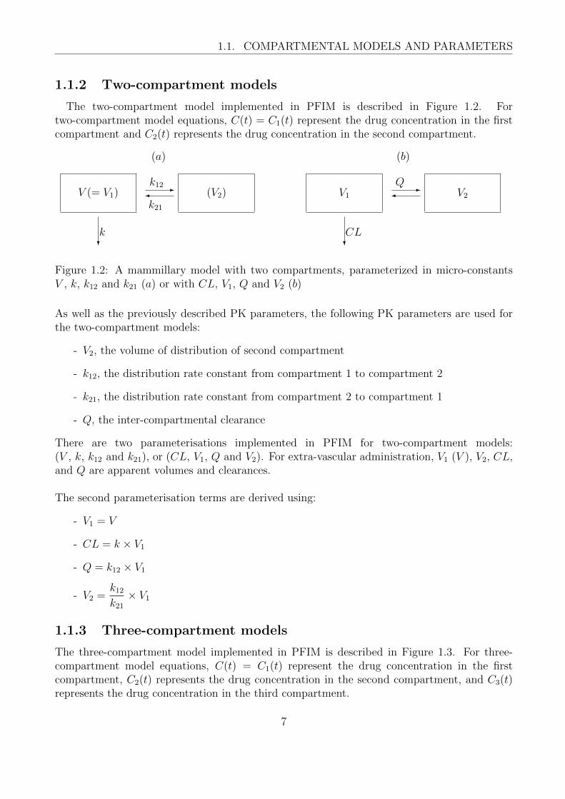
1.1.2 Two-compartment models
The two-compartment model implemented in PFIM is described in Figure 1.2. Fortwo-compartment model equations, C(t) = C1(t) represent the drug concentration in the firstcompartment and C2(t) represents the drug concentration in the second compartment.
-�
?
k12
k21
k
V (= V1) (V2)
(a)
-�
?
Q
CL
V1 V2
(b)
Figure 1.2: A mammillary model with two compartments, parameterized in micro-constantsV , k, k12 and k21 (a) or with CL, V1, Q and V2 (b)
As well as the previously described PK parameters, the following PK parameters are used forthe two-compartment models:
- V2, the volume of distribution of second compartment
- k12, the distribution rate constant from compartment 1 to compartment 2
- k21, the distribution rate constant from compartment 2 to compartment 1
- Q, the inter-compartmental clearance
There are two parameterisations implemented in PFIM for two-compartment models:(V , k, k12 and k21), or (CL, V1, Q and V2). For extra-vascular administration, V1 (V ), V2, CL,and Q are apparent volumes and clearances.
The second parameterisation terms are derived using:
- V1 = V
- CL = k × V1
- Q = k12 × V1
- V2 =k12k21
× V1
1.1.3 Three-compartment models
The three-compartment model implemented in PFIM is described in Figure 1.3. For three-compartment model equations, C(t) = C1(t) represent the drug concentration in the firstcompartment, C2(t) represents the drug concentration in the second compartment, and C3(t)represents the drug concentration in the third compartment.
7

1.1. COMPARTMENTAL MODELS AND PARAMETERS
V (= V1)
?k
(V2)
@@@R@@@Ik21 k12
(V3)
������
�
k13 k31
(a)
V1
?CL
V2
@@@R@@
@IQ2
V3
������
�
Q3
(b)
Figure 1.3: A mammillary model with three compartments parameterized in micro-constantsV , k, k12, k21, k13 and k31 (a) or with CL, V1, Q2, V2, Q3 and V3 (b)
As well as the previously described PK parameters, the following PK parameters are used forthe three-compartment models:
- V3, the volume of distribution of third compartment
- k13, the distribution rate constant from compartment 1 to compartment 3
- k31, the distribution rate constant from compartment 3 to compartment 1
- Q2 (=Q), the inter-compartmental clearance from compartment 1 to compartment 2
- Q3, the inter-compartmental clearance from compartment 1 to compartment 3
There are two parameterisations implemented in PFIM for three-compartment models: (V , k,k12, k21, k13 and k31), or (CL, V1, Q2, V2, Q3 and V3). For extra-vascular administration, V1(V ), V2, V3, CL, Q2, and Q3 are apparent volumes and clearances.
The second parameterisation terms are derived using:
- V1 = V
- CL = k × V1
- Q2 = k12 × V1
- V2 =k12k21
× V1
- Q3 = k13 × V1
- V3 =k13k31
× V1
8

1.2. MODELS WITH LINEAR ELIMINATION
NB: For models with Michaelis-Menten elimination the elimination parameter is not k (orCL) but Vm and Km for both parameterisations of one, two or three-compartment models.
1.2 Models with linear elimination
The list of PK models with linear elimination implemented in PFIM are summarised inAppendix I.1.
1.2.1 One-compartment models
1.2.1.1 Intravenous bolus
• single dose
C (t) =D
Ve−k(t−tD) (1.1)
• multiple doses
C (t) =n∑i=1
Di
Ve−k(t−tDi) (1.2)
• steady state
C(t) =D
V
e−k(t−tD)
1 − e−kτ(1.3)
1.2.1.2 Infusion
• single dose
C (t) =
D
Tinf
1
kV
(1 − e−k(t−tD)
)if t− tD ≤ Tinf ,
D
Tinf
1
kV
(1 − e−kT inf
)e−k(t−tD−T inf) if not.
(1.4)
• multiple doses
C (t) =
n−1∑i=1
Di
Tinfi
1
kV
(1 − e−kT infi
)e−k(t−tDi
−T infi)
+Dn
Tinfn
1
kV
(1 − e−k(t−tDn )
) if t− tDn ≤ Tinfn,
n∑i=1
Di
Tinfi
1
kV
(1 − e−kT infi
)e−k(t−tDi
−T infi) if not.
(1.5)
9
1.2. MODELS WITH LINEAR ELIMINATION
• steady state
C (t) =
D
Tinf
1
kV
[(1 − e−k(t−tD)
)+ e−kτ
(1 − e−kT inf
)e−k(t−tD−T inf)
1 − e−kτ
]if (t− tD) ≤ Tinf ,
D
Tinf
1
kV
(1 − e−kT inf
)e−k(t−tD−T inf)
1 − e−kτif not.
(1.6)
1.2.1.3 First order absorption
• single dose
C (t) =D
V
kaka − k
(e−k(t−tD) − e−ka(t−tD)
)(1.7)
• multiple doses
C (t) =n∑i=1
Di
V
kaka − k
(e−k(t−tDi) − e−ka(t−tDi)
)(1.8)
• steady state
C (t) =D
V
kaka − k
(e−k(t−tD)
1 − e−kτ− e−ka(t−tD)
1 − e−kaτ
)(1.9)
NB: Equations 1.1 to 1.9 correspond to models n◦1 to n◦6 in Appendix I.1.
1.2.2 Two-compartment models
For readability, the equations for two-compartment models with linear elimination are givenusing the variables α, β, A and B defined by the following expressions:
- α =k21k
β=
Q
V2
CL
V1β
- β =
1
2
[k12 + k21 + k −
√(k12 + k21 + k)2 − 4k21k
]1
2
QV1
+Q
V2+CL
V1−
√(Q
V1+Q
V2+CL
V1
)2
− 4Q
V2
CL
V1
The link between A and B, and the PK parameters of the first and second parameterisationsdepends on the input and are given in each subsection.
10

1.2. MODELS WITH LINEAR ELIMINATION
1.2.2.1 Intravenous bolus
For intravenous bolus, the link between A and B, and the parameters (V , k, k12 and k21), or(CL, V1, Q and V2) is defined as follows:
- A =1
V
α− k21α− β
=1
V1
α− Q
V2α− β
- B =1
V
β − k21β − α
=1
V1
β − Q
V2β − α
• single dose
C (t) = D(Ae−α(t−tD) +Be−β(t−tD)
)(1.10)
• multiple doses
C (t) =n∑i=1
Di
(Ae−α(t−tDi) +Be−β(t−tDi)
)(1.11)
• steady state
C (t) = D
(Ae−αt
1 − e−ατ+
Be−βt
1 − e−βτ
)(1.12)
1.2.2.2 Infusion
For infusion, the link between A and B, and the parameters (V , k, k12 and k21), or (CL, V1, Qand V2) is defined as follows:
- A =1
V
α− k21α− β
=1
V1
α− Q
V2α− β
- B =1
V
β − k21β − α
=1
V1
β − Q
V2β − α
• single dose
C (t) =
D
Tinf
A
α
(1 − e−α(t−tD)
)+B
β
(1 − e−β(t−tD)
) if t− tD ≤ Tinf ,
D
Tinf
A
α
(1 − e−αTinf
)e−α(t−tD−T inf)
+B
β
(1 − e−βT inf
)e−β(t−tD−T inf)
if not.
(1.13)
11

1.2. MODELS WITH LINEAR ELIMINATION
• multiple doses
C (t) =
n−1∑i=1
Di
Tinfi
A
α
(1 − e−αTinfi
)e−α(t−tDi
−T infi)
+B
β
(1 − e−βT infi
)e−β(t−tDi
−T infi)
+D
Tinfn
A
α
(1 − e−α(t−tDn )
)+B
β
(1 − e−β(t−tDn )
)
if t− tDn ≤ Tinf ,
n∑i=1
Di
Tinfi
A
α
(1 − e−αTinfi
)e−α(t−tDi
−T infi)
+B
β
(1 − e−βT infi
)e−β(t−tDi
−T infi)
if not.
(1.14)
• steady state
C (t) =
D
Tinf
A
α
(1 − e−α(t−tD)
)+ e−ατ
(1 − e−αTinf
)e−α(t−tD−T inf)
1 − e−ατ
+B
β
(1 − e−β(t−tD)
)+ e−βτ
(1 − e−βT inf
)e−β(t−tD−T inf)
1 − e−βτ
if t− tD ≤ Tinf ,
D
Tinf
A
α
((1 − e−αTinf
)e−α(t−tD−T inf)
1 − e−ατ
)
+B
β
((1 − e−βT inf
)e−β(t−tD−T inf)
1 − e−βτ
) if not.
(1.15)
1.2.2.3 First order absorption
For first order absorption, the link between A and B, and the parameters (ka, V , k, k12 andk21), or (ka, CL, V1, Q and V2) is defined as follows:
- A =kaV
k21 − α
(ka − α) (β − α)=kaV1
Q
V2− α
(ka − α) (β − α)
- B =kaV
k21 − β
(ka − β) (α− β)=kaV1
Q
V2− β
(ka − β) (α− β)
12

1.2. MODELS WITH LINEAR ELIMINATION
• single dose
C (t) = D(Ae−α(t−tD) +Be−β(t−tD) − (A+B)e−ka(t−tD)
)(1.16)
• multiple doses
C (t) =n∑i=1
Di
(Ae−α(t−tDi) +Be−β(t−tDi) − (A+B)e−ka(t−tDi)
)(1.17)
• steady state
C (t) = D
(Ae−α(t−tD)
1 − e−ατ+Be−β(t−tD)
1 − e−βτ− (A+B)e−ka(t−tD)
1 − e−kaτ
)(1.18)
NB: Equations 1.10 to 1.18 correspond to models n◦7 to n◦12 in Appendix I.1.
1.2.3 Three-compartment models
For readability, the equations for three-compartment models with linear elimination are givenusing the variables α, β, γ, A, B and C defined by the following expressions:
- a0 = kk21k31 =CL
V1
Q2
V2
Q3
V3
- a1 =
kk31 + k21k31 + k21k13 + kk21 + k31k12
CL
V1
Q3
V3+Q2
V2
Q3
V3+Q2
V2
Q3
V1+CL
V1
Q2
V2+Q3
V3
Q2
V1
- a2 =
k + k12 + k13 + k21 + k31
CL
V1+Q2
V1+Q3
V1+Q2
V2+Q3
V3
- p = a1 − a22/3
- q = 2a32/27 − a1a2/3 + a0
- r1 =√− (p3/27)
- r2 = 2r1/31
- φ = arccos
(− q
2r1
)/3
- α = − (cos (φ) r2 − a2/3)
- β = −(
cos
(φ+
2π
3
)r2 − a2/3
)13

1.2. MODELS WITH LINEAR ELIMINATION
- γ = −(
cos
(φ+
4π
3
)r2 − a2/3
)The link between A, B, C and the PK parameters of the first and second parameterisationsdepends on the input and are given in each subsection.
1.2.3.1 Intravenous bolus
For intravenous bolus, the link between A B, and C, and the parameters (V , k, k12, k21, k13and k31), or (CL, V1, Q2, V2, Q3 and V3) is defined as follows:
- A =1
V
k21 − α
α− β
k31 − α
α− γ=
1
V1
Q2
V2− α
α− β
Q3
V3− α
α− γ
- B =1
V
k21 − β
β − α
k31 − β
β − γ=
1
V1
Q2
V2− β
β − α
Q3
V3− β
β − γ
- C =1
V
k21 − γ
γ − β
k31 − γ
γ − α=
1
V1
Q2
V2− γ
γ − β
Q3
V3− γ
γ − α
• single dose
C (t) = D(Ae−α(t−tD) +Be−β(t−tD) + Ce−γ(t−tD)
)(1.19)
• multiple doses
C (t) =n∑i=1
Di
(Ae−α(t−tDi) +Be−β(t−tDi) + Ce−γ(t−tDi)
)(1.20)
• steady state
C (t) = D
(Ae−α(t−tD)
1 − e−ατ+Be−β(t−tD)
1 − e−βτ+Ce−γ(t−tD)
1 − e−γτ
)(1.21)
1.2.3.2 Infusion
For infusion, the link between A B, and C, and the parameters (V , k, k12, k21, k13 and k31), or(CL, V1, Q2, V2, Q3 and V3) is defined as follows:
- A =1
V
k21 − α
α− β
k31 − α
α− γ=
1
V1
Q2
V2− α
α− β
Q3
V3− α
α− γ
- B =1
V
k21 − β
β − α
k31 − β
β − γ=
1
V1
Q2
V2− β
β − α
Q3
V3− β
β − γ
14

1.2. MODELS WITH LINEAR ELIMINATION
- C =1
V
k21 − γ
γ − β
k31 − γ
γ − α=
1
V1
Q2
V2− γ
γ − β
Q3
V3− γ
γ − α
• single dose
C (t) =
D
Tinf
A
α
(1 − e−α(t−tD)
)+B
β
(1 − e−β(t−tD)
)+C
γ
(1 − e−γ(t−tD)
)
if t− tD ≤ Tinf ,
D
Tinf
A
α
(1 − e−αTinf
)e−α(t−tD−T inf)
+B
β
(1 − e−βT inf
)e−β(t−tD−T inf)
+C
γ
(1 − e−γT inf
)e−γ(t−tD−T inf)
if not.
(1.22)
• multiple doses
C (t) =
n−1∑i=1
Di
Tinfi
A
α
(1 − e−αTinfi
)e−α(t−tDi
−T infi)
+B
β
(1 − e−βT infi
)e−β(t−tDi
−T infi)
+C
γ
(1 − e−γT infi
)e−γ(t−tDi
−T infi)
+D
Tinfn
A
α
(1 − e−α(t−tDn )
)+B
β
(1 − e−β(t−tDn )
)+C
γ
(1 − e−γ(t−tDn )
)
if t− tDn ≤ Tinf ,
n∑i=1
Di
Tinfi
A
α
(1 − e−αTinfi
)e−α(t−tDi
−T infi)
+B
β
(1 − e−βT infi
)e−β(t−tDi
−T infi)
+C
γ
(1 − e−γT infi
)e−γ(t−tDi
−T infi)
if not.
(1.23)
15

1.2. MODELS WITH LINEAR ELIMINATION
• steady state
C (t) =
D
Tinf
A
α
(1 − e−α(t−tD)
)+ e−ατ
(1 − e−αTinf
)e−α(t−tD−T inf)
1 − e−ατ
+B
β
(1 − e−β(t−tD)
)+ e−βτ
(1 − e−βT inf
)e−β(t−tD−T inf)
1 − e−βτ
+C
γ
(1 − e−γ(t−tD)
)+ e−γτ
(1 − e−γT inf
)e−γ(t−tD−T inf)
1 − e−γτ
if t− tD ≤ Tinf ,
D
Tinf
A
α
((1 − e−αTinf
)e−α(t−tD−T inf)
1 − e−ατ
)
+B
β
((1 − e−βT inf
)e−β(t−tD−T inf)
1 − e−βτ
)
+C
γ
((1 − e−γT inf
)e−γ(t−tD−Tinf)
1 − e−γτ
)
if not.
(1.24)
1.2.3.3 First order absorption
For first order absorption, the link between A B, and C, and the parameters (ka, V , k, k12,k21, k13 and k31), or (ka, CL, V1, Q2, V2, Q3 and V3) is defined as follows:
- A =1
V
kaka − α
k21 − α
α− β
k31 − α
α− γ=
1
V1
kaka − α
Q2
V2− α
α− β
Q3
V3− α
α− γ
- B =1
V
kaka − β
k21 − β
β − α
k31 − β
β − γ=
1
V1
kaka − β
Q2
V2− β
β − α
Q3
V3− β
β − γ
- C =1
V
kaka − γ
k21 − γ
γ − β
k31 − γ
γ − α=
1
V1
kaka − γ
Q2
V2− γ
γ − β
Q3
V3− γ
γ − α
• single dose
C (t) = D(Ae−α(t−tD) +Be−β(t−tD) + Ce−γ(t−tD) − (A+B + C)e−ka(t−tD)
)(1.25)
• multiple doses
C (t) =n∑i=1
Di
(Ae−α(t−tDi) +Be−β(t−tDi) + Ce−γ(t−tDi) − (A+B + C)e−ka(t−tDi)
)(1.26)
16

1.3. MODELS WITH MICHAELIS-MENTEN ELIMINATION
• steady state
C (t) = D
(Ae−α(t−tD)
1 − e−ατ+Be−β(t−tD)
1 − e−βτ+Ce−γ(t−tD)
1 − e−γτ− (A+B + C)e−ka(t−tD)
1 − e−kaτ
)(1.27)
NB: Equations 1.19 to 1.27 correspond to models n◦13 to n◦18 in Appendix I.1.
1.3 Models with Michaelis-Menten elimination
The list of PK models with Michaelis-Menten elimination implemented in PFIM are summarisedin Appendix I.2. Presently, there is no implementation for multiple dosing with IV bolusadministration in the PFIM software. For infusion and oral administration, the implementationin PFIM does not allow designs with different groups of doses as the dose is included in themodel.
1.3.1 One-compartment models
1.3.1.1 Intravenous bolus
• single dose
Initial conditions:
C (t) = 0 for t < tD
C (tD) =D
V
dC
dt= −
VmV
× C
Km + C
(1.28)
1.3.1.2 Infusion
• single dose
Initial conditions: C (t) = 0 for t < tD
dC
dt= −
VmV
× C
Km + C+ input
input (t) =
D
Tinf
1
Vif 0 ≤ t− tD ≤ Tinf
0 if not.
(1.29)
17

1.3. MODELS WITH MICHAELIS-MENTEN ELIMINATION
• multiple doses
Initial conditions: C (t) = 0 for t < tD1
dC
dt= −
VmV
× C
Km + C+ input
input (t) =
Di
Tinfi
1
Vif 0 ≤ t− tDi
≤ Tinfi,
0 if not.
(1.30)
1.3.1.3 First order absorption
• single dose
Initial conditions: C (t) = 0 for t < tD
dC
dt= −
VmV
× C
Km + C+ input
input (t) =D
Vkae
−ka(t−tD)
(1.31)
• multiple doses
Initial conditions: C (t) = 0 for t < tD1
dC
dt= −
VmV
× C
Km + C+ input
input (t) =n∑i=1
Di
Vkae
−ka(t−tDi)
(1.32)
NB: Equations 1.28 to 1.32 correspond to model n◦1 to n◦3 in Appendix I.2.
18

1.3. MODELS WITH MICHAELIS-MENTEN ELIMINATION
1.3.2 Two-compartment models
1.3.2.1 Intravenous bolus
• single dose
Initial conditions:
C1 (t) = 0 for t < tD
C2 (t) = 0 for t ≤ tD
C1 (tD) =D
V
dC1
dt= −
VmV
× C1
Km + C1
− k12C1 +k21V2V
C2
dC2
dt=k12V
V2C1 − k21C2
(1.33)
1.3.2.2 Infusion
• single dose
Initial conditions:
{C1 (t) = 0 for t < tD
C2 (t) = 0 for t ≤ tD
dC1
dt= −
VmV
× C1
Km + C1
− k12C1 +k21V2V
C2 + input
dC2
dt=k12V
V2C1 − k21C2
input (t) =
D
Tinf
1
Vif 0 ≤ t− tD ≤ Tinf
0 if not.
(1.34)
• multiple doses
Initial conditions:
{C1 (t) = 0 for t < tD1
C2 (t) = 0 for t ≤ tD1
dC1
dt= −
VmV
× C1
Km + C1
− k12C1 +k21V2V
C2 + input
dC2
dt=k12V
V2C1 − k21C2
input (t) =
Di
Tinfi
1
Vif 0 ≤ t− tDi
≤ Tinfi,
0 if not.
(1.35)
19

1.3. MODELS WITH MICHAELIS-MENTEN ELIMINATION
1.3.2.3 First order absorption
• single dose
Initial conditions:
{C1 (t) = 0 for t < tD
C2 (t) = 0 for t ≤ tD
dC1
dt= −
VmV
× C1
Km + C1
− k12C1 +k21V2V
C2 + input
dC2
dt=k12V
V2C1 − k21C2
input (t) =D
Vkae
−ka(t−tD)
(1.36)
• multiple doses
Initial conditions:
{C1 (t) = 0 for t < tD1
C2 (t) = 0 for t ≤ tD1
dC1
dt= −
VmV
× C1
Km + C1
− k12C1 +k21V2V
C2 + input
dC2
dt=k12V
V2C1 − k21C2
input (t) =n∑i=1
Di
Vkae
−ka(t−tDi)
(1.37)
NB: Equations 1.33 to 1.37 correspond to models n◦4 to n◦9 in Appendix I.2.
20
1.3. MODELS WITH MICHAELIS-MENTEN ELIMINATION
1.3.3 Three-compartment models
1.3.3.1 Intravenous bolus
• single dose
Initial conditions:
C1 (t) = 0 for t < tD
C2 (t) = 0 for t ≤ tD
C3 (t) = 0 for t ≤ tD
C1 (tD) =D
V
dC1
dt= −
VmV
× C1
Km + C1
− k12C1 +k21V2V
C2 − k13C1 +k31V3V
C3
dC2
dt=
k12V
V2C1 − k21C2
dC3
dt=
k13V
V3C1 − k31C3
(1.38)
1.3.3.2 Infusion
• single dose
Initial conditions:
C1 (t) = 0 for t < tD
C2 (t) = 0 for t ≤ tD
C3 (t) = 0 for t ≤ tD
dC1
dt= −
VmV
× C1
Km + C1
− k12C1 +k21V2V
C2 − k13C1 +k31V3V
C3 + input
dC2
dt=
k12V
V2C1 − k21C2
dC3
dt=
k13V
V3C1 − k31C3
input (t) =
D
Tinf
1
Vif 0 ≤ t− tD ≤ Tinf
0 if not.
(1.39)
21

1.3. MODELS WITH MICHAELIS-MENTEN ELIMINATION
• multiple doses
Initial conditions:
C1 (t) = 0 for t < tD1
C2 (t) = 0 for t ≤ tD1
C3 (t) = 0 for t ≤ tD1
dC1
dt= −
VmV
× C1
Km + C1
− k12C1 +k21V2V
C2 − k13C1 +k31V3V
C3 + input
dC2
dt=
k12V
V2C1 − k21C2
dC3
dt=
k13V
V3C1 − k31C3
input (t) =
Di
Tinfi
1
Vif 0 ≤ t− tDi
≤ Tinfi,
0 if not.
(1.40)
1.3.3.3 First order absorption
• single dose
Initial conditions:
C1 (t) = 0 for t < tD
C2 (t) = 0 for t ≤ tD
C3 (t) = 0 for t ≤ tD
dC1
dt= −
VmV
× C1
Km + C1
− k12C1 +k21V2V
C2 − k13C1 +k31V3V
C3 + input
dC2
dt=
k12V
V2C1 − k21C2
dC3
dt=
k13V
V3C1 − k31C3
input (t) =D
Vkae
−ka(t−tD)
(1.41)
22

1.3. MODELS WITH MICHAELIS-MENTEN ELIMINATION
• multiple doses
Initial conditions:
C1 (t) = 0 for t < tD1
C2 (t) = 0 for t ≤ tD1
C3 (t) = 0 for t ≤ tD1
dC1
dt= −
VmV
× C1
Km + C1
− k12C1 +k21V2V
C2 − k13C1 +k31V3V
C3 + input
dC2
dt=
k12V
V2C1 − k21C2
dC3
dt=
k13V
V3C1 − k31C3
input (t) =n∑i=1
Di
Vkae
−ka(t−tDi)
(1.42)
NB: Equations 1.38 to 1.42 correspond to models n◦10 to n◦15 in Appendix I.2.
23
Chapter 2
Pharmacodynamic models
This chapter describes the pharmacodynamic models implemented in the PFIM software. Someof these pharmacodynamic models can be used alone or linked to a pharmacokinetic model.Some can only be used linked to any pharmacokinetic model. Two different types of modelsare presented here:
• The immediate response models (alone or linked to a pharmacokinetic model)
• The turnover models (only linked to a pharmacokinetic model)
The list of the immediate response models implemented in PFIM is summarised in AppendixII.1 and II.2. The list of the turnover models is summarised in Appendix II.3.
2.1 Immediate response models
For these response models, the effect E (t) is expressed as:
E (t) = A (t) + S (t) (2.1)
where A (t) represents the model of drug action and S (t) corresponds to the baseline/diseasemodel. A (t) is a function of the concentration C (t) in the central compartment.
The drug action models are presented in section 2.1.1 for C(t). The baseline/disease modelsare presented in section 2.1.2. Any combination of those two models is available in the PFIMlibrary.
Parameters
• Alin: constant associated to C (t)
• Aquad: constant associated to the square of C (t)
• Alog: constant associated to the logarithm of C (t)
• Emax: maximal agonistic response
• Imax: maximal antagonistic response
24

2.1. IMMEDIATE RESPONSE MODELS
• C50: concentration to get half of the maximal response (i.e. drug potency)
• γ: sigmoidicity factor
• S0: baseline value of the studied effect
• kprog: rate constant of disease progression
2.1.1 Drug action models
• linear model
A (t) = AlinC (t) (2.2)
• quadratic model
A (t) = AlinC (t) + AquadC (t)2 (2.3)
• logarithmic model
A (t) = Aloglog(C (t)) (2.4)
• Emax model
A (t) =EmaxC (t)
C (t) + C50
(2.5)
• sigmoıd Emax model
A (t) =EmaxC (t)γ
C (t)γ + Cγ50
(2.6)
• Imax model
A (t) = 1 − ImaxC (t)
C (t) + C50
(2.7)
• sigmoıd Imax model
A (t) = 1 − ImaxC (t)γ
C (t)γ + Cγ50
(2.8)
25

2.1. IMMEDIATE RESPONSE MODELS
2.1.2 Baseline/disease models
• null baseline
S (t) = 0 (2.9)
• constant baseline with no disease progression
S (t) = S0 (2.10)
• linear disease progression
S (t) = S0 + kprogt (2.11)
• exponential disease increase
S (t) = S0e−kprogt (2.12)
• exponential disease decrease
S (t) = S0
(1 − e−kprogt
)(2.13)
NB: Only, for the Imax models (equation (2.7) and (2.8)) A (t) is not added to S (t) but S0
is multiplied by A (t) in the expression of S(t).
2.1.3 PFIM model function examples
Any combination of the 9 drug action models and 5 baseline/disease models is available inPFIM. For instance, the combination of an Emax model for the drug action (2.5) and a constantbaseline with no disease progression model (2.10) will result in the following equation:
E(t) = S0 +EmaxC (t)
C (t) + C50
(2.14)
which corresponds to the model n◦11: immed Emax const in Appendix II.1.
As a second example, the combination of an Imax model for the drug action (2.7) with aexponential progression as baseline/disease model (2.12) will give:
E(t) = S0
(e−kprogt − ImaxC (t)
C (t) + C50
)(2.15)
which corresponds to the model n◦13: immed Imax exp in Appendix II.2.
26
2.2. TURNOVER RESPONSE MODELS
2.2 Turnover response models
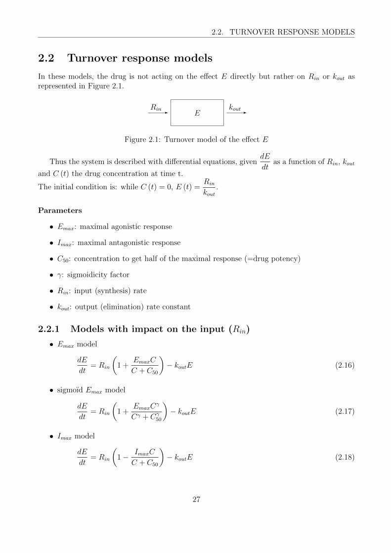
In these models, the drug is not acting on the effect E directly but rather on Rin or kout asrepresented in Figure 2.1.
-Rin -
koutE
Figure 2.1: Turnover model of the effect E
Thus the system is described with differential equations, givendE
dtas a function of Rin, kout
and C (t) the drug concentration at time t.
The initial condition is: while C (t) = 0, E (t) =Rin
kout.
Parameters
• Emax: maximal agonistic response
• Imax: maximal antagonistic response
• C50: concentration to get half of the maximal response (=drug potency)
• γ: sigmoidicity factor
• Rin: input (synthesis) rate
• kout: output (elimination) rate constant
2.2.1 Models with impact on the input (Rin)
• Emax model
dE
dt= Rin
(1 +
EmaxC
C + C50
)− koutE (2.16)
• sigmoıd Emax model
dE
dt= Rin
(1 +
EmaxCγ
Cγ + Cγ50
)− koutE (2.17)
• Imax model
dE
dt= Rin
(1 − ImaxC
C + C50
)− koutE (2.18)
27
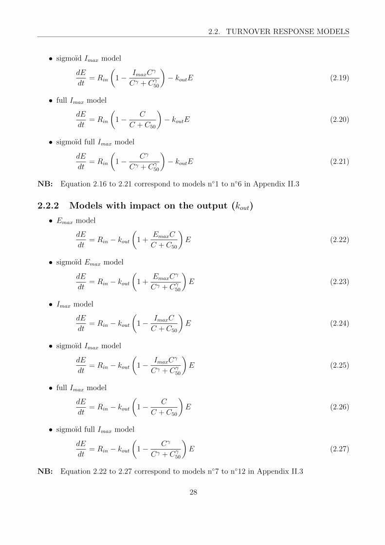
2.2. TURNOVER RESPONSE MODELS
• sigmoıd Imax model
dE
dt= Rin
(1 − ImaxC
γ
Cγ + Cγ50
)− koutE (2.19)
• full Imax model
dE
dt= Rin
(1 − C
C + C50
)− koutE (2.20)
• sigmoıd full Imax model
dE
dt= Rin
(1 − Cγ
Cγ + Cγ50
)− koutE (2.21)
NB: Equation 2.16 to 2.21 correspond to models n◦1 to n◦6 in Appendix II.3
2.2.2 Models with impact on the output (kout)
• Emax model
dE
dt= Rin − kout
(1 +
EmaxC
C + C50
)E (2.22)
• sigmoıd Emax model
dE
dt= Rin − kout
(1 +
EmaxCγ
Cγ + Cγ50
)E (2.23)
• Imax model
dE
dt= Rin − kout
(1 − ImaxC
C + C50
)E (2.24)
• sigmoıd Imax model
dE
dt= Rin − kout
(1 − ImaxC
γ
Cγ + Cγ50
)E (2.25)
• full Imax model
dE
dt= Rin − kout
(1 − C
C + C50
)E (2.26)
• sigmoıd full Imax model
dE
dt= Rin − kout
(1 − Cγ
Cγ + Cγ50
)E (2.27)
NB: Equation 2.22 to 2.27 correspond to models n◦7 to n◦12 in Appendix II.3
28

Appendix
List and names of the PK and PD models available in PFIM (PFIM since version3.2.1 and PFIM Interface since version 3.1)
Appendix I: list of models in PK library
For the use in the PFIM software, some variables are required (or not) for each PK model.They are specified in the column named Needed variables: N: the number of doses, tau: theinterval between two doses, TInf: the duration of the infusion, doseMM: dose for models withMichaelis-Menten elimination (for models with linear elimination, dose is specified in the filestdin.r).
29

2.2. TURNOVER RESPONSE MODELS
Appendix I.1: PK models with linear elimination
30

2.2. TURNOVER RESPONSE MODELS
31

2.2. TURNOVER RESPONSE MODELS
Appendix I.2: PK models with Michaelis-Menten elimination
32

2.2. TURNOVER RESPONSE MODELS
Appendix II: list of models in PD library
The implementation of the PD models in the PFIM software differs if the PD model is usedalone or linked to a pharmacokinetic model. The immediate response models used alone aredescribed in Appendix II.1. The list of the immediate response PD models for PK/PD is thusgiven in Appendix II.1 plus those of Appendix II.2. Lastly, the list of turnover PD models forPK/PD is given in Appendix II.3.
For the case where a PK model with linear elimination is associated to a turnover PD responsemodel, the PK model is written with a differential equations system. Consequently, only somePK models from Appendix I.1 are implemented:
- for IV bolus, only single dose models
- for infusion and oral absorption, single dose and multiple doses
33

2.2. TURNOVER RESPONSE MODELS
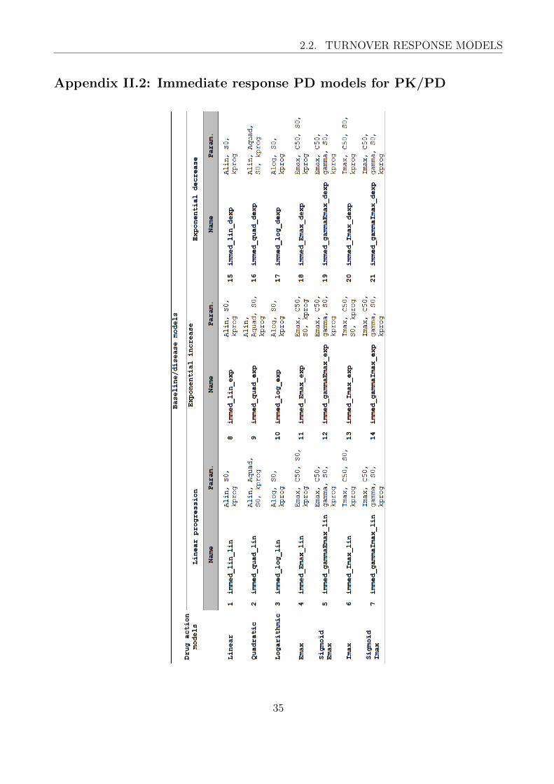
Appendix II.1: Immediate response PD models for PD only
34
2.2. TURNOVER RESPONSE MODELS
Appendix II.2: Immediate response PD models for PK/PD
35

2.2. TURNOVER RESPONSE MODELS
Appendix II.3: Turnover PD models for PK/PD
36