Embed Size (px)
Citation preview
ISSN 1937 - 1055
VOLUME 3, 2021
INTERNATIONAL JOURNAL OF
MATHEMATICAL COMBINATORICS
EDITED BY
THE MADIS OF CHINESE ACADEMY OF SCIENCES AND
ACADEMY OF MATHEMATICAL COMBINATORICS & APPLICATIONS, USA
September, 2021
Vol.3, 2021 ISSN 1937-1055
International Journal of
Mathematical Combinatorics
(http://fs.unm.edu/IJMC.htm, www.mathcombin.com/IJMC.htm)
Edited By
The Madis of Chinese Academy of Sciences and
Academy of Mathematical Combinatorics & Applications, USA
September, 2021
Aims and Scope: The mathematical combinatorics is a subject that applying combinatorial
notion to all mathematics and all sciences for understanding the reality of things in the universe,
motivated by CC Conjecture of Dr.Linfan MAO on mathematical sciences. The International
J.Mathematical Combinatorics (ISSN 1937-1055) is a fully refereed international journal,
sponsored by the MADIS of Chinese Academy of Sciences and published in USA quarterly,
which publishes original research papers and survey articles in all aspects of mathematical
combinatorics, Smarandache multi-spaces, Smarandache geometries, non-Euclidean geometry,
topology and their applications to other sciences. Topics in detail to be covered are:
Mathematical combinatorics;
Smarandache multi-spaces and Smarandache geometries with applications to other sciences;
Topological graphs; Algebraic graphs; Random graphs; Combinatorial maps; Graph and
map enumeration; Combinatorial designs; Combinatorial enumeration;
Differential Geometry; Geometry on manifolds; Low Dimensional Topology; Differential
Topology; Topology of Manifolds;
Geometrical aspects of Mathematical Physics and Relations with Manifold Topology;
Mathematical theory on gravitational fields and parallel universes;
Applications of Combinatorics to mathematics and theoretical physics.
Generally, papers on applications of combinatorics to other mathematics and other sciences
are welcome by this journal.
It is also available from the below international databases:
Serials Group/Editorial Department of EBSCO Publishing
10 Estes St. Ipswich, MA 01938-2106, USA
Tel.: (978) 356-6500, Ext. 2262 Fax: (978) 356-9371
http://www.ebsco.com/home/printsubs/priceproj.asp
and
Gale Directory of Publications and Broadcast Media, Gale, a part of Cengage Learning
27500 Drake Rd. Farmington Hills, MI 48331-3535, USA
Tel.: (248) 699-4253, ext. 1326; 1-800-347-GALE Fax: (248) 699-8075
http://www.gale.com
Indexing and Reviews: Mathematical Reviews (USA), Zentralblatt Math (Germany), Index
EuroPub (UK), Referativnyi Zhurnal (Russia), Mathematika (Russia), EBSCO (USA), Google
Scholar, Baidu Scholar, Directory of Open Access (DoAJ), International Scientific Indexing
(ISI, impact factor 2.012), Institute for Scientific Information (PA, USA), Library of Congress
Subject Headings (USA), CNKI(China).
Subscription A subscription can be ordered by an email directly to
Linfan Mao
The Editor-in-Chief of International Journal of Mathematical CombinatoricsChinese Academy of Mathematics and System Science Beijing, 100190, P.R.China, and also thePresident of Academy of Mathematical Combinatorics & Applications (AMCA), Colorado, USA
Email: [email protected]
Price: US$48.00
Editorial Board (4th)
Editor-in-Chief
Linfan MAO
Chinese Academy of Mathematics and System
Science, P.R.China
and
Academy of Mathematical Combinatorics &
Applications, Colorado, USA
Email: [email protected]
Deputy Editor-in-Chief
Guohua Song
Beijing University of Civil Engineering and
Architecture, P.R.China
Email: [email protected]
Editors
Arindam Bhattacharyya
Jadavpur University, India
Email: [email protected]
Said Broumi
Hassan II University Mohammedia
Hay El Baraka Ben M’sik Casablanca
B.P.7951 Morocco
Junliang Cai
Beijing Normal University, P.R.China
Email: [email protected]
Yanxun Chang
Beijing Jiaotong University, P.R.China
Email: [email protected]
Jingan Cui
Beijing University of Civil Engineering and
Architecture, P.R.China
Email: [email protected]
Shaofei Du
Capital Normal University, P.R.China
Email: [email protected]
Xiaodong Hu
Chinese Academy of Mathematics and System
Science, P.R.China
Email: [email protected]
Yuanqiu Huang
Hunan Normal University, P.R.China
Email: [email protected]
H.Iseri
Mansfield University, USA
Email: [email protected]
Xueliang Li
Nankai University, P.R.China
Email: [email protected]
Guodong Liu
Huizhou University
Email: [email protected]
W.B.Vasantha Kandasamy
Indian Institute of Technology, India
Email: [email protected]
Ion Patrascu
Fratii Buzesti National College
Craiova Romania
Han Ren
East China Normal University, P.R.China
Email: [email protected]
Ovidiu-Ilie Sandru
Politechnica University of Bucharest
Romania
ii International Journal of Mathematical Combinatorics
Mingyao Xu
Peking University, P.R.China
Email: [email protected]
Guiying Yan
Chinese Academy of Mathematics and System
Science, P.R.China
Email: [email protected]
Y. Zhang
Department of Computer Science
Georgia State University, Atlanta, USA
Famous Words:
We must accept finite disappointment, but we never lose infinite hope.
By Mattin Luther King, a leader of the American civil rights
International J.Math. Combin. Vol.3(2021), 1-19
Reality with Smarandachely Denied Axiom
Linfan MAO
1. Chinese Academy of Mathematics and System Science, Beijing 100190, P.R.China
2. Academy of Mathematical Combinatorics & Applications (AMCA), Colorado, USA
E-mail: [email protected]
Abstract: Usually, one applies mathematics to hold on the reality of matters in the uni-
verse, i.e., mathematical reality and a few peoples firmly believe that classical mathematics
could handle this things with no needs on its extension. However, it is not the case be-
cause contradictions exist everywhere but classical mathematics must be logically consistent
without contradiction in the eyes of human beings. The fatal flaw in this view is it’s priori
assumption that the universe is uniform, and then can be characterized by homogeneous
characters with classical mathematics such as differential equations. However, the universe
including its matters are not uniform, even being messy. This fact implies that one should
extend classical mathematics to an enveloping one for understanding matters in the universe
and bearing maybe with contradictions, i.e., such systems in mathematics including with
Smarandachely denied axioms. Certainly, an axiom is said Smarandachely denied if the ax-
iom behaves differently, i.e., validated and invalided, or only invalidated but in at least two
distinct ways in a system S. Such a system S is said Smarandace system. The main purpose
of this paper is to introduce the Smarandachely denied axiom, show its contribution to re-
ality and explain the role of its equivalent form, the Smarandache multispace for extending
classical mathematics, i.e., mathematical combinatorics for understanding matters because
each matter always inherits a topological structure by its nature in the universe.
Key Words: Reality, mathematical reality, CC conjecture, mathematical universe hypoth-
esis, Smarandachely denied axiom, Smarandache system, Smarandache multispace, mathe-
matical combinatorics.
AMS(2010): 03A05,03A10,05C22,51-02,70-02.
§1. Introduction
Usually, all matter in the universe are colorful, maybe with mystery and complex mechanism to
the human eyes no matter it is living or not. We understand matters by the reality for promoting
the survival and development of humans ourselves in harmony with nature. However, we are
embarrassed hardly know their true face unless their surface characters before humans and even
so, it could be also a false vision or hallucination, just feelings of humans. Then, what is the
reality of a matter? The word reality of a matter T is its state as it actually exist, including
everything that is and has been, no matter it is observable or comprehensible by humans. For
1Received June 5, 2021, Accepted August 25, 2021.
2 Linfan MAO
humans ourselves, a natural question is could we really hold on the reality of matters in the
universe? It should be noted that the answer is different in the scientific and the religious. For
examples, all matters are illusion of humans claimed by Sakyamuni in his famous Diamond
Sutra and the universal truth can be restated but the restated truth is not the universal one
asserted by Laozi in his Tao Te Ching. However, nearly all scientists firmly believe that we can
open the cover enveloped on matters, find their true face and then, hold on the natural laws of
universe. Here, we do not discuss who’s right or who’s wrong. Even if we can really open the
cover on matters in the universe, there is also a question on reality, i.e., how to characterize the
reality of matters? The answer is nothing else but the science or particularly, the mathematical
sciences.
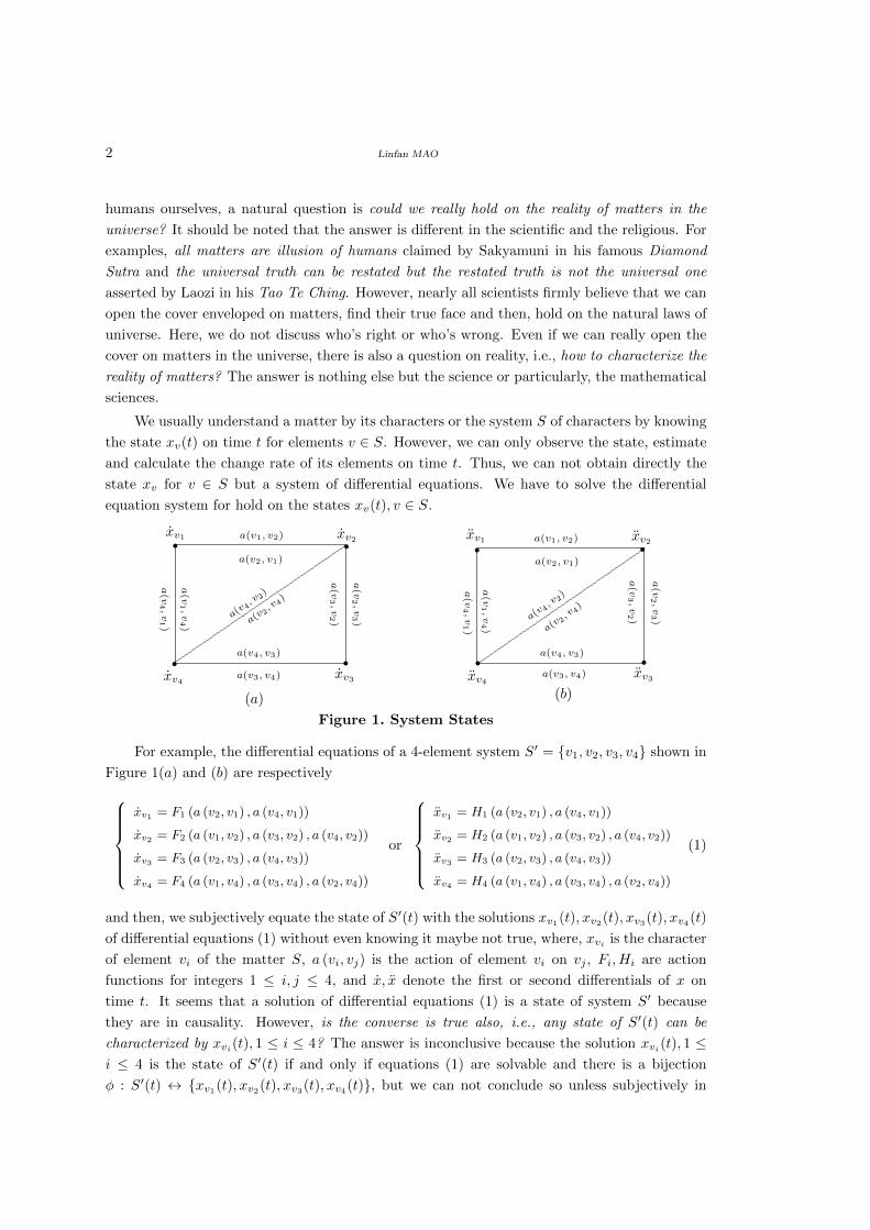
We usually understand a matter by its characters or the system S of characters by knowing
the state xv(t) on time t for elements v ∈ S. However, we can only observe the state, estimate
and calculate the change rate of its elements on time t. Thus, we can not obtain directly the
state xv for v ∈ S but a system of differential equations. We have to solve the differential
equation system for hold on the states xv(t), v ∈ S.
r r r r
r r
a(v1, v2)
a(v2, v1)
a(v1, v2)
a(v2, v1)
a(v
2,v3)
a(v
3,v2)
a(v3, v4)
a(v4, v3)
a(v
4,v1)
a(v
1,v4)
a(v4, v
2)
a(v2, v
4)
a(v
2,v3)
a(v
3,v2)
a(v3, v4)
a(v4, v3)
a(v
4,v1)
a(v
1,v4)
a(v4, v
2)
a(v2, v
4)
xv1 xv2
xv3xv4
xv1 xv2
xv3xv4
rr(a) (b)
Figure 1. System States
For example, the differential equations of a 4-element system S′ = {v1, v2, v3, v4} shown in
Figure 1(a) and (b) are respectivelyxv1 = F1 (a (v2, v1) , a (v4, v1))
xv2 = F2 (a (v1, v2) , a (v3, v2) , a (v4, v2))
xv3 = F3 (a (v2, v3) , a (v4, v3))
xv4 = F4 (a (v1, v4) , a (v3, v4) , a (v2, v4))
or
xv1 = H1 (a (v2, v1) , a (v4, v1))
xv2 = H2 (a (v1, v2) , a (v3, v2) , a (v4, v2))
xv3 = H3 (a (v2, v3) , a (v4, v3))
xv4 = H4 (a (v1, v4) , a (v3, v4) , a (v2, v4))
(1)
and then, we subjectively equate the state of S′(t) with the solutions xv1(t), xv2(t), xv3(t), xv4(t)
of differential equations (1) without even knowing it maybe not true, where, xvi is the character
of element vi of the matter S, a (vi, vj) is the action of element vi on vj , Fi, Hi are action
functions for integers 1 ≤ i, j ≤ 4, and x, x denote the first or second differentials of x on
time t. It seems that a solution of differential equations (1) is a state of system S′ because
they are in causality. However, is the converse is true also, i.e., any state of S′(t) can be
characterized by xvi(t), 1 ≤ i ≤ 4? The answer is inconclusive because the solution xvi(t), 1 ≤i ≤ 4 is the state of S′(t) if and only if equations (1) are solvable and there is a bijection
φ : S′(t) ↔ {xv1(t), xv2(t), xv3(t), xv4(t)}, but we can not conclude so unless subjectively in
Reality with Smarandachely Denied Axiom 3
mind on classical mathematics. Certainly, a mathematical system should be logically consistent
without contradiction but lots of humans misunderstand this criterion, excluded contradictory
systems in mathematics, which results in the limitation of mathematics on reality of matters.
It should be noted that the most important thing is not excluded contradictions but how to let
them coexist peacefully in mathematics for extending the limitation of classical mathematics
and establish an envelope mathematics, in which classical mathematics only be its parts for
understanding matters in the universe. For this objective, the Smarandachely denied axiom is
a such one presented by F.Smarandache on geometry in 1969 following ([37],[40-41]).
Axiom 1.1 An axiom is said Smarandachely denied if in the same space the axiom behaves
differently, i.e., validated and invalided, or only invalidated but in at least two distinct ways.
By Axiom 1.1, there are Smarandachely conceptions on geometry following.
Definition 1.2([16],[37]) A Smarandache geometry is such a geometry that has at least one
Smarandachely denied axiom.
A conception closely related to Smarandache geometry is the Smarandache multispace
defined in the following, which seems to be a generalization of Smarandache geometry but
equivalent to Smarandache geometry by a geometrical view.
Definition 1.3([17],[37]) Let (Σ1;R1), (Σ2;R2), · · · , (Σm;Rm) be m mathematical spaces,
different two by two, i.e., for any two spaces (Σi;Ri) and (Σj ;Rj), Σi 6= Σj or Σi = Σj but
Ri 6= Rj. A Smarandache multispace Σ is a unionm⋃i=1
Σi with rules R =m⋃i=1
Ri on Σ, i.e., the
union of rules Ri on Σi for integers 1 ≤ i ≤ m, denoted by(
Σ; R)
.
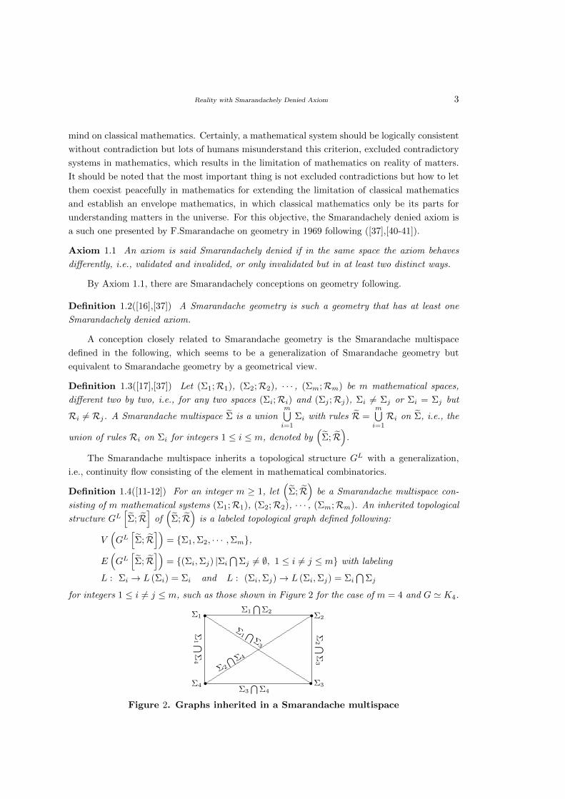
The Smarandache multispace inherits a topological structure GL with a generalization,
i.e., continuity flow consisting of the element in mathematical combinatorics.
Definition 1.4([11-12]) For an integer m ≥ 1, let(
Σ; R)
be a Smarandache multispace con-
sisting of m mathematical systems (Σ1;R1), (Σ2;R2), · · · , (Σm;Rm). An inherited topological
structure GL[Σ; R
]of(
Σ; R)
is a labeled topological graph defined following:
V(GL[Σ; R
])= {Σ1,Σ2, · · · ,Σm},
E(GL[Σ; R
])= {(Σi,Σj) |Σi
⋂Σj 6= ∅, 1 ≤ i 6= j ≤ m} with labeling
L : Σi → L (Σi) = Σi and L : (Σi,Σj)→ L (Σi,Σj) = Σi⋂
Σj
for integers 1 ≤ i 6= j ≤ m, such as those shown in Figure 2 for the case of m = 4 and G ' K4.r r
r r
Σ1 Σ2
Σ3Σ4
Σ1
⋂Σ2
Σ3
⋂Σ4
Σ2 ⋂
Σ3
Σ1 ⋂
Σ4
Σ2
⋂ Σ4
Σ1⋂Σ3
Figure 2. Graphs inherited in a Smarandache multispace
4 Linfan MAO
Now, what is the contribution of Axiom 1.1 in extending of classical mathematics and what
is its role with the reality? The main purpose of this paper is to introduce the Smarandachely
denied axiom, survey its contribution to geometry, and then from Smarandache multispace to
mathematical combinatorics for extending classical mathematics to mathematical combinatorics
for understanding the reality of matters in the universe because each matter always inherits a
topological structure by its nature.
For terminologies and notations not mentioned here, we follow reference [4] for algebra, [5]
for topological graphs, [16-18] and [37-38] for Smarandache geometry, multispaces and Smaran-
dache systems.
§2. Smarandachely Denied Axiom to Geometry
Notice that the Smarandachely denied axiom is originally presented on geometry, which enables
one to generalize geometry to Smarandache geometry concluding classical geometry as its parts.
In a Smarandache geometry, the points, lines, planes, spaces, triangles, · · · are respectively
called s-points, s-lines, s-planes, s-spaces, s-triangles, · · · in order to distinguish them from
those in classical geometry. Although it is defined by Definition 1.2, an elementary but natural
question is shown in the following.
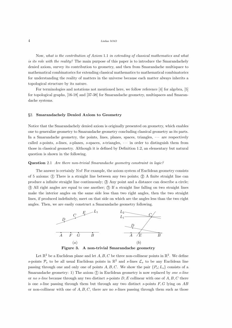
Question 2.1 Are there non-trivial Smarandache geometry constraint in logic?
The answer is certainly Yes! For example, the axiom system of Euclidean geometry consists
of 5 axioms: 1© There is a straight line between any two points; 2© A finite straight line can
produce a infinite straight line continuously; 3© Any point and a distance can describe a circle;
4© All right angles are equal to one another; 5© If a straight line falling on two straight lines
make the interior angles on the same side less than two right angles, then the two straight
lines, if produced indefinitely, meet on that side on which are the angles less than the two right
angles. Then, we are easily construct a Smarandache geometry following.
qq qq qq q
A B
C
F G
D
E
(a)
L1 qqq q
C
A E B
(b)
L1
L2
qD
Figure 3. A non-trivial Smarandache geometry
Let R2 be a Euclidean plane and let A,B,C be three non-collinear points in R2. We define
s-points Ps to be all usual Euclidean points in R2 and s-lines Ls to be any Euclidean line
passing through one and only one of points A,B,C. We show the pair {Ps;Ls} consists of a
Smarandache geometry: 1) The axiom 1© in Euclidean geometry is now replaced by one s-line
or no s-line because through any two distinct s-points D,E collinear with one of A,B,C there
is one s-line passing through them but through any two distinct s-points F,G lying on AB
or non-collinear with one of A,B,C, there are no s-lines passing through them such as those
Reality with Smarandachely Denied Axiom 5
shown in Figure 3(a); 2) The axiom 5© is now replaced by one parallel or no parallel because if
we let L1, L2 be two s-lines passing through C with L1 parallel but L2 not parallel to AB in
the Euclidean sense, then through any s-point D not lying on AB there are no s-lines parallel
to L1 but there is one s-lines parallel to L2 if one of DB,DA or DC happens parallel to L2.
Otherwise, there are no s-lines passing through D parallel to L2, see Figure 3(b) for details.
More examples of Smarandache geometry can be found in [3], [6-7], [10] and [40-41]. Cer-
tainly, the quantitative characterization on the real face of matters lead to the neutrosophic
logic by Smarandachely denied axiom, which contributes the introduction of the degree of nega-
tion or partial negation of an axiom and, more general, of a scientific or humanistic proposition
(theorem, lemma, etc.) in any field. It works somehow like the negation in fuzzy logic with a
degree of truth, a degree of falsehood and a degree of truth, i.e. neither truth nor falsehood
but unknown, ambiguous, indeterminate (see [40-41] for details).
As a particular case, the Euclidean, Lobachevsky-Bolyai-Gauss and Riemannian geometries
may be united altogether by the Smarandache geometry in the same space because it can be
partially Euclidean and partially non-Euclidean, and it seems connecting with the relativity
theory and parallel universes because it includes the Riemannian geometry in a subspace but
more generalized. H.Iseri [6-7] constructed the Smarandache 2-manifolds by using equilateral
triangular disks on Euclidean plane R2, which can be come true by paper models in R3 for
elliptic, Euclidean and hyperbolic cases and in paper [10], L.Mao advanced a new method for
constructed Smarandache 2-manifold by combinatorial maps. Generally, it should be noted that
Smarandache n-manifold for n ≥ 2, i.e. combinatorial n-manifold and a differential theory on
such manifolds were constructed by L.Mao in papers [11]. For n = 1, i.e., a curve in differential
geometry is called Smarandache curve if it holds with Smarandachely denied axiom, which
has been extensively researched and many researching, such as those of papers [2],[9],[36],[42]-
[47], [50] were published in the International Journal of Mathematical Combinatorics after it
suggested by L.Mao for the authors of [44]. In fact, nearly all geometries in classical mathematics
such as those of Riemann geometry, Finsler geometry, Weyl geometry and Kahler geometry are
particular cases of Smarandache geometry.
§3. Smarandachely Denied Axiom to Mathematical Systems
Although the Smarandachely denied axiom is originally to geometry for generalizing the 5th
axiom of Euclidean geometry. Its notion can be generalized further to a generalized form on all
mathematical systems by replacing the word space with mathematical system following.
Axiom 3.1(Generalized Smarandachely denied axiom) An axiom is said generalized Smaran-
dachely denied if in the same mathematical system the axiom behaves differently, i.e., validated
and invalided, or only invalidated but in at least two distinct ways and then, a Smarandache
system is such a mathematical system that has at least one Smarandachely denied axiom.
For example, a Lie group G in classical mathematics is a Smarandachely denied system
because an element a ∈ G is both a point on manifold G, also an element in group G. Thus,
if we let Axiom I be an axiom that points have no neighborhood C on G, Axiom II be that
6 Linfan MAO
a−1 is not exist for ∀a ∈ G and Axiom III to be that the group operations (a, b) → a · b or
a → a−1 are not C∞-mapping. Then, Axioms I, II and III are invalidated in a Lie group,
which implies G is a Smarandache system and in general, the result following can be verified.
Proposition 3.2 Let (S1,R1) , (S2,R2) , · · · , (Sn,Rn) be n systems in classical mathematics
with Si 6= Sj or Si = Sj but Ri 6= Rj for an integers n ≥ 2, where Si is a set, Ri ⊂ Si ×Si for
integers 1 ≤ i ≤ n. Then, the union
(Σ; Π) = (S1 ∪ S2 ∪ · · · ∪ Sn;R1 ∪R2 ∪ · · · ∪ Rn)
is a Smarandache system.
Proof Similarly to the case of Lie group, define Axiom i to be (a, b) 6∈ Ri for ∀a, b ∈ Siin (Σ; Π) if (a, b) ∈ Ri in (Si,Ri) for integers 1 ≤ i ≤ n. Then, each Axiom i is invalidated in
(Σ; Π), i.e., invalidated in at least two distinct ways. �
Notice that the Smarandache system(S; R
)in Proposition 3.2 is in fact a Smarandache
multispace by Definition 1.3, appearing not only in mathematics but also in physics, for in-
stance the unmatter composed of particles and anti-particles [39], and generally, the generalized
Smarandachely denied axiom is equivalent to Smarandache multispace.
Proposition 3.3 A mathematical system (Σ,Π) is generalized Smarandachely denied if and
only if it is a Smarandache multispace.
Proof The proof on necessity of the result is similar to the decomposition shown in [22],
divided into two cases following.
Case 1. There is an axiom A in (Σ,Π) that behaves both validated and invalided. Define
Σ1 = {x ∈ Σ hold with Axiom A }, Σ2 = {y ∈ Σ hold not with Axiom A }.
Then, Σ = Σ1
⋃Σ2, i.e., (Σ,Π) is a Smarandache multispace.
Case 2. There is an axiom in A in (Σ,Π) that behaves invalidated but in distinct ways
W1,W2, · · · ,Ws, s ≥ 2. Define Σi = {x ∈ Σ hold not with Axiom A in way Wi} for integers
1 ≤ i ≤ s and Σ0 = Σ\s⋃i=1
Σi, where Σ0 maybe an empty set. Then
Σ =
(n⋃i=1
Σi
)⋃Σ0 (3)
is a Smarandache multispace.
The proof on sufficiency of the result is similar to the proof of Proposition 3.2. Let (Σ,Π) be
a Smarandache multispace with Σ = Σ1
⋃Σ2
⋃· · ·⋃
Σn, Π = R1
⋃R2
⋃· · ·⋃Rn and (Σi;Ri)
being a mathematical space. Define Axiom Ai = {x 6∈ Σi if x ∈ Σi} for integers 1 ≤ i ≤ n.
Then, each axiom Ai in Σ behaves both validated, invalided, and also invalidated in n distinct
ways. �
Notice that there are many achievements of Smarandache multispaces in extending clas-
sical mathematics with applying to physics. For example, multigroups, multirings, multifields,
multialgebra and multistructure,· · · , etc. discussed in [1], [14]-[15], [17] and [48]-[49].
Reality with Smarandachely Denied Axiom 7
§4. Smarandachely Denied Axiom to Reality
4.1. Mathematical Reality. Proposition 3.3 enables one to discuss the reality of matters in
the universe by generalized Smarandachely denied axiom. Particularly, the reality discussed by
differential equations in physics, i.e., the mathematical reality is the reality on a matter or not.
The conclusion following is a little surprising for the usual view on classical mathematics.
Proposition 4.1 If RM , R are respectively the mathematical reality or the reality of a matter
in the universe. Then RM ⊆ R and furthermore, there are many examples hold with RM 6= R.
Proof The relation RM ⊆ R is obvious. For the inequality RM 6= R, many cases show the
mathematical reality is not the reality, even the ridiculous on reality of a matter in sometimes,
for instance the equations (1) are non-solvable, i.e., we can not obtain the state of system S′(t).
Even the equations (1) are solvable, we can not conclude their solutions describing the state
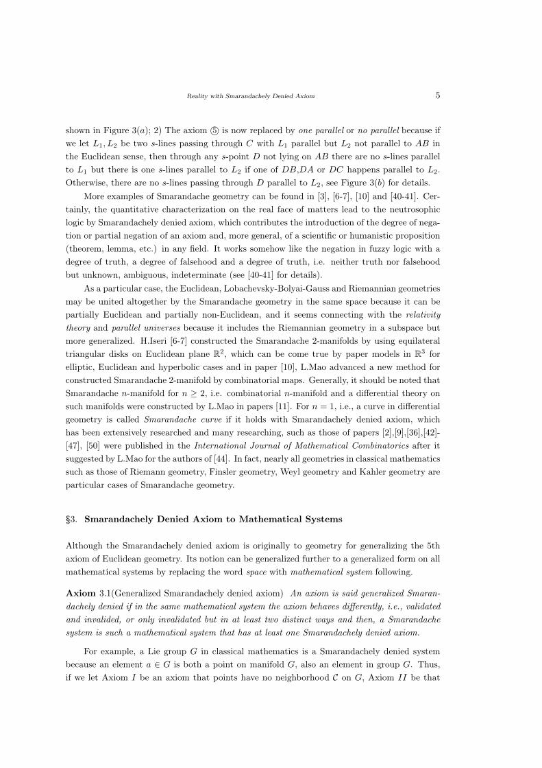
of system S′. For example, let H1, H2, H3, H4 and H ′1, H′2, H
′3, H
′4 be two groups of running
horses constraint with running on respectively 4 straight lines
1©
x+ y = 2
x+ y = −2
x− y = −2
x− y = 2
or 2©
x = y
x+ y = 2
x = 1
y = 1
on the Euclidean plane R2 such as those shown in Figure 4(a), (b) and (c).
Figure 4. Four horses on the plane
Clearly, the first system is non-solvable because x+ y = −2 is contradictious to x+ y = 2,
and so that for the equation x − y = −2 to x − y = 2 but the second system is solvable with
(x, y) = (1, 1). Could we conclude that the running states of horses H ′1, H′2, H
′3, H
′4 are a point
(1, 1), i.e., staying on the point (1, 1) and H1, H2, H3, H4 are nothing? The answer is certainly
not because all of the horses are running on the Euclidean plane R2. However, we know nothing
on the state by the solution of the two equation systems because the solvability of systems 1©or 2© only implies the orbits intersection, not the running state of the group of horses. �
Then, what is wrong in the example of the two groups of horses? The wrong appears
with the assumption that the solution of 1© or 2© characterizes the running state of horses
8 Linfan MAO
H ′1, H′2, H
′3, H
′4 or H1, H2, H3, H4. Certainly, each equation in systems 1© or 2© really charac-
terizes the running state of one horse but we can not equate the running states of the four horses
with the solution of 1© and 2© because they are different in objective, and maybe contradictory.
Generally, there is contradiction maybe if we characterize a group of matters within a same s-
pace. Indeed, we can eliminate the contradiction by characterizing them with different variables
of spaces, for instance in parallel spaces one by one. However, they are really a system with
relations on its elements, we should know their global state of the system, not isolated one on
its elements in the Euclidean plane R2. This case implies also that the non-solvable systems of
equations characterize matters also if each of them was established on the characters of matters
in the universe but the solution is not the state of the matter when it consists of characters more
than 2, which implies the classical mathematics is incomplete for understanding the reality of
matters, particularly, the biological systems in the universe.
Notice that a cosmologist, Max Tegmark proposed a hypothesis on the universe once, called
the mathematical universe hypothesis following, spread widely in the scientific community.
Hypothesis 4.2(Max Tegmark,[47]) The physical universe is not merely described by mathe-
matics but a mathematical structure, i.e., RM = R.
Certainly, the mathematical universe hypothesis is essentially a duplication of the Theory
of Everything. However, Proposition 4.1 concludes classical mathematics is incomplete for
understanding matters in the unverse, which implies that the incorrectness of the mathematical
universe hypothesis, or in other words, the first step to making this hypothesis work should
be the extending of classical mathematics, i.e., including contradictions, let them peaceful
coexistence in mathematics, and then it maybe set up on the universe.
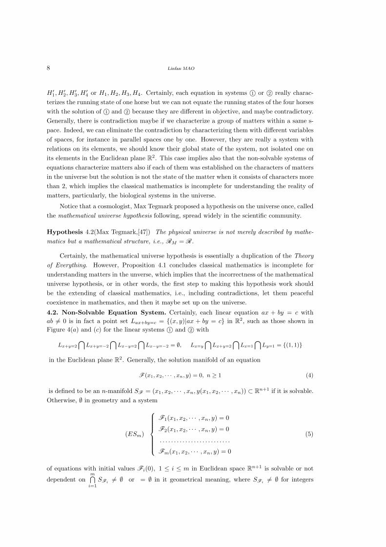
4.2. Non-Solvable Equation System. Certainly, each linear equation ax + by = c with
ab 6= 0 is in fact a point set Lax+by=c = {(x, y)|ax + by = c} in R2, such as those shown in
Figure 4(a) and (c) for the linear systems 1© and 2© with
Lx+y=2
⋂Lx+y=−2
⋂Lx−y=2
⋂Lx−y=−2 = ∅, Lx=y
⋂Lx+y=2
⋂Lx=1
⋂Ly=1 = {(1, 1)}
in the Euclidean plane R2. Generally, the solution manifold of an equation
F (x1, x2, · · · , xn, y) = 0, n ≥ 1 (4)
is defined to be an n-manifold SF = (x1, x2, · · · , xn, y(x1, x2, · · · , xn)) ⊂ Rn+1 if it is solvable.
Otherwise, ∅ in geometry and a system
(ESm)
F1(x1, x2, · · · , xn, y) = 0
F2(x1, x2, · · · , xn, y) = 0
. . . . . . . . . . . . . . . . . . . . . . . . .
Fm(x1, x2, · · · , xn, y) = 0
(5)
of equations with initial values Fi(0), 1 ≤ i ≤ m in Euclidean space Rn+1 is solvable or not
dependent onm⋂i=1
SFi6= ∅ or = ∅ in it geometrical meaning, where SFi
6= ∅ for integers
Reality with Smarandachely Denied Axiom 9
1 ≤ i ≤ m.
Then, what is the reality of a matter T ? Generally, let µ1, µ2, · · · , µn be known and νi, i ≥ 1
unknown characters at time t for a matter T . Then, T should be understood by
T =
(n⋃i=1
{µi}
)⋃⋃k≥1
{νk}
(6)
in logic but with an approximation T ◦ =n⋃i=1
{µi} for T by humans at time t, which is nothing
else but the Smarandache system or multispace by Proposition 3.3. The example of 4 horses
run in the plane shows that applying the solution of equations (5), i.e.,m⋂i=1
SFito the state of
a system S maybe cause a ridiculous conclusion, particularly in the case of the non-solvable.
In fact, the state of a matter T described by the system equation (5) is notm⋂i=1
SFi but the
equality (6), i.e., Smarandache multispace. We should extend the conception of solution of
equations (5).
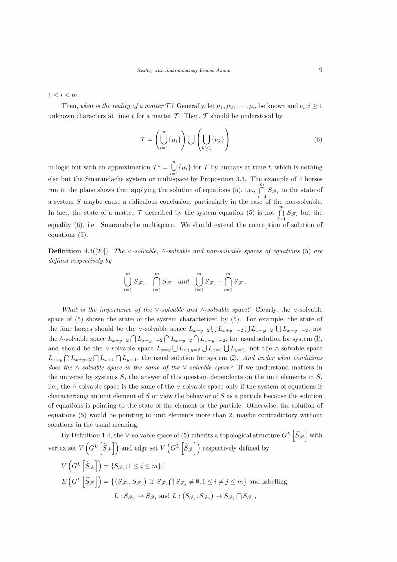
Definition 4.3([20]) The ∨-solvable, ∧-solvable and non-solvable spaces of equations (5) are
defined respectively by
m⋃i=1
SFi,
m⋂i=1
SFiand
m⋃i=1
SFi−
m⋂i=1
SFi.
What is the importance of the ∨-solvable and ∧-solvable space? Clearly, the ∨-solvable
space of (5) shown the state of the system characterized by (5). For example, the state of
the four horses should be the ∨-solvable space Lx+y=2
⋃Lx+y=−2
⋃Lx−y=2
⋃Lx−y=−2, not
the ∧-solvable space Lx+y=2
⋂Lx+y=−2
⋂Lx−y=2
⋂Lx−y=−2, the usual solution for system 1©,
and should be the ∨-solvable space Lx=y
⋃Lx+y=2
⋃Lx=1
⋃Ly=1, not the ∧-solvable space
Lx=y
⋂Lx+y=2
⋂Lx=1
⋂Ly=1, the usual solution for system 2©. And under what conditions
does the ∧-solvable space is the same of the ∨-solvable space? If we understand matters in
the universe by systems S, the answer of this question dependents on the unit elements in S,
i.e., the ∧-solvable space is the same of the ∨-solvable space only if the system of equations is
characterizing an unit element of S or view the behavior of S as a particle because the solution
of equations is pointing to the state of the element or the particle. Otherwise, the solution of
equations (5) would be pointing to unit elements more than 2, maybe contradictory without
solutions in the usual meaning.
By Definition 1.4, the ∨-solvable space of (5) inherits a topological structure GL[SF
]with
vertex set V(GL[SF
])and edge set V
(GL[SF
])respectively defined by
V(GL[SF
])= {SFi
; 1 ≤ i ≤ m};
E(GL[SF
])={(SFi
, SFj
)if SFi
⋂SFj
6= ∅, 1 ≤ i 6= j ≤ m}
and labelling
L : SFi→ SFi
and L :(SFi
, SFj
)→ SFi
⋂SFj
,
10 Linfan MAO
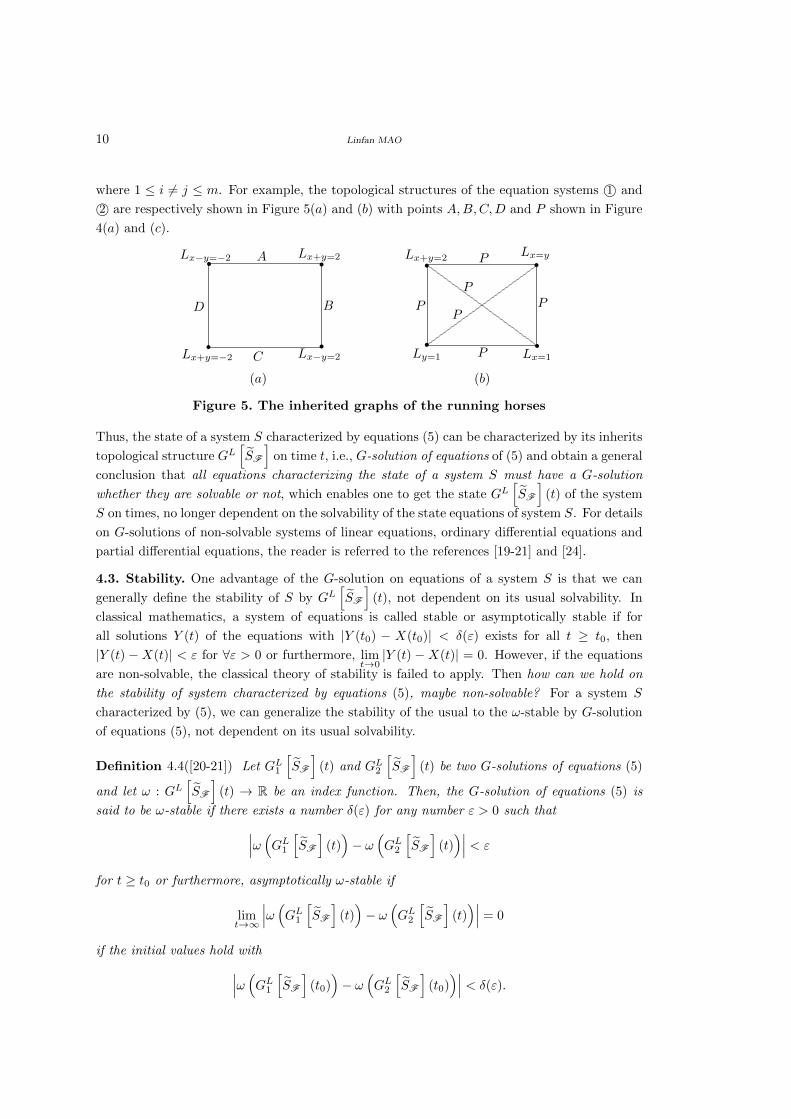
where 1 ≤ i 6= j ≤ m. For example, the topological structures of the equation systems 1© and
2© are respectively shown in Figure 5(a) and (b) with points A,B,C,D and P shown in Figure
4(a) and (c).
A
B
C
D
Lx−y=−2 Lx+y=2
Lx−y=2Lx+y=−2
r r
rr
r r
rr
Lx+y=2Lx=y
Lx=1Ly=1
P
P
P
P
P
P
(a) (b)
Figure 5. The inherited graphs of the running horses
Thus, the state of a system S characterized by equations (5) can be characterized by its inherits
topological structure GL[SF
]on time t, i.e., G-solution of equations of (5) and obtain a general
conclusion that all equations characterizing the state of a system S must have a G-solution
whether they are solvable or not, which enables one to get the state GL[SF
](t) of the system
S on times, no longer dependent on the solvability of the state equations of system S. For details
on G-solutions of non-solvable systems of linear equations, ordinary differential equations and
partial differential equations, the reader is referred to the references [19-21] and [24].
4.3. Stability. One advantage of the G-solution on equations of a system S is that we can
generally define the stability of S by GL[SF
](t), not dependent on its usual solvability. In
classical mathematics, a system of equations is called stable or asymptotically stable if for
all solutions Y (t) of the equations with |Y (t0) − X(t0)| < δ(ε) exists for all t ≥ t0, then
|Y (t) −X(t)| < ε for ∀ε > 0 or furthermore, limt→0|Y (t) −X(t)| = 0. However, if the equations
are non-solvable, the classical theory of stability is failed to apply. Then how can we hold on
the stability of system characterized by equations (5), maybe non-solvable? For a system S
characterized by (5), we can generalize the stability of the usual to the ω-stable by G-solution
of equations (5), not dependent on its usual solvability.
Definition 4.4([20-21]) Let GL1
[SF
](t) and GL2
[SF
](t) be two G-solutions of equations (5)
and let ω : GL[SF
](t) → R be an index function. Then, the G-solution of equations (5) is
said to be ω-stable if there exists a number δ(ε) for any number ε > 0 such that∣∣∣ω (GL1 [SF
](t))− ω
(GL2
[SF
](t))∣∣∣ < ε
for t ≥ t0 or furthermore, asymptotically ω-stable if
limt→∞
∣∣∣ω (GL1 [SF
](t))− ω
(GL2
[SF
](t))∣∣∣ = 0
if the initial values hold with∣∣∣ω (GL1 [SF
](t0)
)− ω
(GL2
[SF
](t0)
)∣∣∣ < δ(ε).
Reality with Smarandachely Denied Axiom 11
If the index function ω is linear, we can further introduce the sum-stability of systems
characterized by equations (5).
Definition 4.5([20-22], [24],[26]) A G-solution is said to be sum-stable or asymptotically sum-
stable if all solutions xi(t), 1 ≤ i ≤ m of equations of (5) exists for t ≥ t0 and∥∥∥∥∥m∑i=1
xi(t)−∑i=1m
yi(t)
∥∥∥∥∥ < ε,
or furthermore,
limt→t0
∥∥∥∥∥m∑i=1
xi(t)−∑i=1m
yi(t)
∥∥∥∥∥ = 0
if ‖xi(t0)− yi(t0)‖ < ε, where, ε > 0 is a real number and ‖X‖ denotes the norm of vector X.
The sum-stability of ordinary differential equations and partial differential equations are
researched in references [17] and [20]. For example, the following result on the sum-stability of
linear ordinary differential equations was obtained.
Theorem 4.5([20-21]) A G-solution of system (5) of linear homogenous differential equations is
asymptotically sum-stable if and only if Reαi < 0 for βi(t)eαit ∈ SFi
, 1 ≤ i ≤ m of linear basis,
where βi(t) is a polynomial of degree less than k− 1 on t if αi is a k-fold root of characteristic
equation of the Fi (x1, x2, · · · , xn, y) = 0.
§5. Mathematical Combinatorics
The mathematical combinatorics is such a subject that applying the combinatorial notion, i.e.
CC Conjecture in [13] to all other mathematics and all other sciences for understanding the
reality of things in the universe, happens to share the same view of Smarandache’s notion,
particularly, the Smarandache multispace by a combinatorial view.
5.1. CC Conjecture. Notice that the Smarandache multispace can be viewed as a combinato-
rial theory because it discuss the combination of spaces not only one as in classical mathematics.
Essentially, the CC conjecture is also a notion for extending classical mathematics presented
by imitating the 2-cell partition on surface initially following.
Conjecture 5.1([13],16) Any mathematical science can be reconstructed from or made by
combinationization.
It should be noted that this conjecture claims that we can select finite combinatorial rulers
and axioms to reconstruct or make generalization for mathematical sciences likewise Euclidean
geometry, abstract groups, vector space or rings such that the mathematics as a combinatorial
generalization of the classical one, and we can make the combinationization of different branches
in mathematics and extend them over topological structures because the classical mathematics
can be viewed as a mathematics over a topological point in space.
12 Linfan MAO
Why is the CC conjecture important for extending classical mathematics? Because of the
limitation of humans ourselves in understanding manner, i.e., only partially or locally under-
standing likewise the philosophical implications in the fable of the blind men and an elephant,
we have to combine all the partially or locally understanding on matters in the universe, and
because the universe is a combinatorial one in human eyes, we should have such a mathematics
going with the understanding manner, i.e., mathematical combinatorics. Then, do we really
need a proof on the CC conjecture? No, not need! Because we have known all matters in the
universe are combined of elementary particles, and all livings are combined of cells and genes. If
we approve the scientific understanding on matters in the universe is by mathematics, then we
should extend classical mathematics to a combinatorial one catering to the understanding man-
ner, i.e., mathematical combinatorics because we can then understand matters form the partial
or local to the global by mathematics. Certainly, there are many achievements for extending
classical mathematics by CC conjecture after it was presented in 2006. For example, combina-
torial Euclidean space, combinatorial Riemannian submanifolds, combinatorial principal fiber
bundles and combinatorial gravitational fields, · · · , etc. are researched. For the contribution of
CC conjecture to classical mathematics, the reader is refereed to [18], which was motivated by
the combinatorial notion, particularly, the CC conjecture.
What is the relation of the CC conjecture with Smarandachely denied axiom? By Proposi-
tion 3.3, the generalized Smarandachely denied axiom is equivalent to the Smarandache systems
on mathematical science and the CC conjecture is a notion on mathematical systems over topo-
logical structures, they are essentially equal but the direction of CC conjecture is a little clearer
on extending classical mathematics because we already have the theory on topological graphs
which is essentially the combinationization of 2-dimensional manifolds ([5], [16], [18]) and we
can apply all achievements in the classical to mathematical combinatorics on elements, i.e.,
continuity flows, i.e., extending elements in classical mathematics over topological structures.
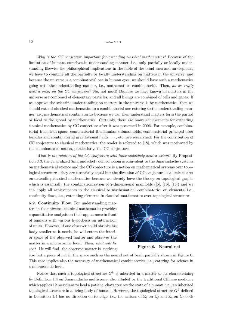
5.2. Continuity Flow. For understanding mat-
ters in the universe, classical mathematics provides
a quantitative analysis on their appearance in front
of humans with various hypothesis on interaction
of units. However, if one observer could shrinks his
body smaller as it needs, he will enters the interi-
or space of the observed matter and observes the
matter in a microcosmic level. Then, what will he
see? He will find the observed matter is nothingFigure 6. Neural net
else but a piece of net in the space such as the neural net of brain partially shown in Figure 6.
This case implies also the necessity of mathematical combinatorics, i.e., catering for science in
a microcosmic level.
Notice that such a topological structure GL is inherited in a matter or its characterizing
by Definition 1.4 on Smarandache multispace, also alluded by the traditional Chinese medicine
which applies 12 meridians to heal a patient, characterizes the state of a human, i.e., an inherited
topological structure in a living body of human. However, the topological structure GL defined
in Definition 1.4 has no direction on its edge, i.e., the actions of Σi on Σj and Σi on Σi both
Reality with Smarandachely Denied Axiom 13
are equal but the flows in the 12 meridians of a human body all have directions and generally,
all actions should have directions in the nature. Whence, we should generalized the topological
structure in Definition 1.4 from no to with directions on edges, constraint with the conservation
laws on all its vertices as flows in nature, which leads to the continuity flows.
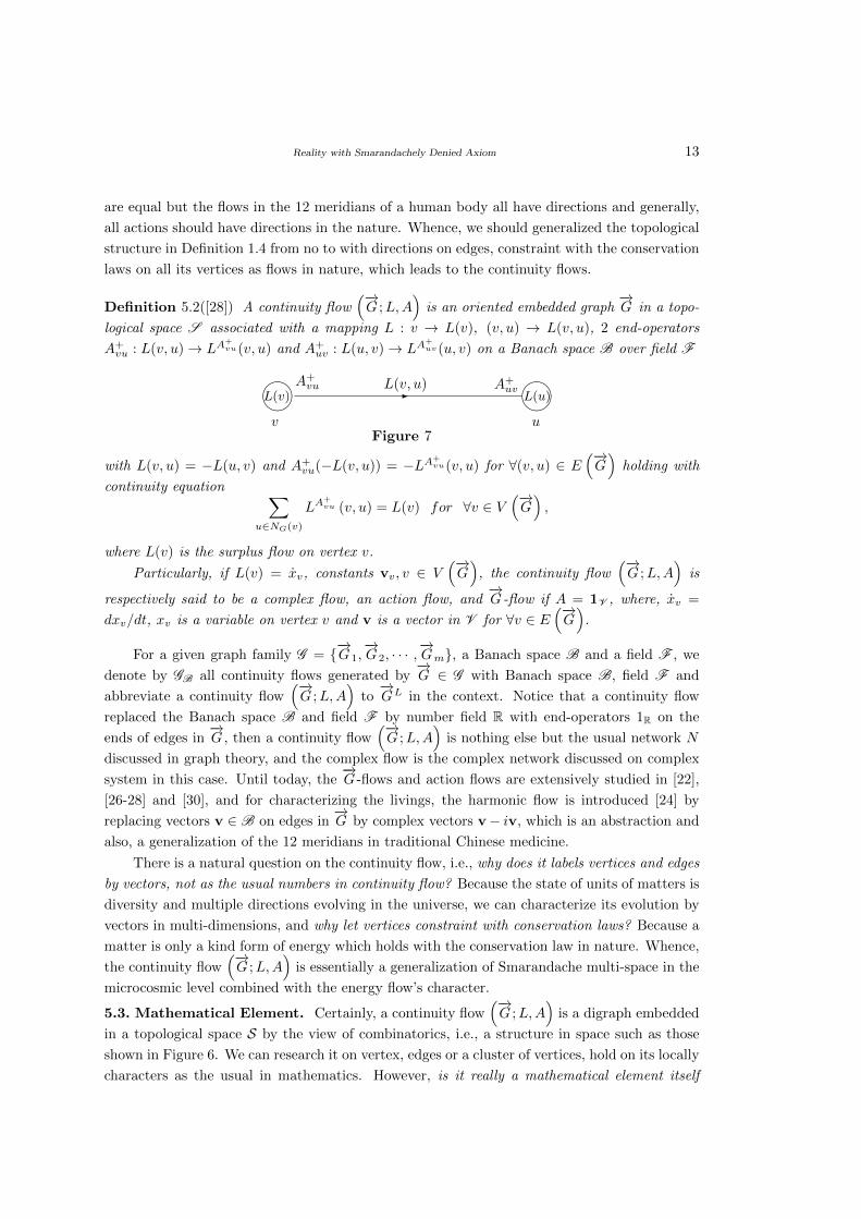
Definition 5.2([28]) A continuity flow(−→G ;L,A
)is an oriented embedded graph
−→G in a topo-
logical space S associated with a mapping L : v → L(v), (v, u) → L(v, u), 2 end-operators
A+vu : L(v, u)→ LA
+vu(v, u) and A+
uv : L(u, v)→ LA+uv (u, v) on a Banach space B over field F
-���� ����L(v, u)A+vu A+
uvL(v) L(u)
v uFigure 7
with L(v, u) = −L(u, v) and A+vu(−L(v, u)) = −LA+
vu(v, u) for ∀(v, u) ∈ E(−→G)
holding with
continuity equation ∑u∈NG(v)
LA+vu (v, u) = L(v) for ∀v ∈ V
(−→G),
where L(v) is the surplus flow on vertex v.
Particularly, if L(v) = xv, constants vv, v ∈ V(−→G)
, the continuity flow(−→G ;L,A
)is
respectively said to be a complex flow, an action flow, and−→G-flow if A = 1V , where, xv =
dxv/dt, xv is a variable on vertex v and v is a vector in V for ∀v ∈ E(−→G)
.
For a given graph family G = {−→G1,−→G2, · · · ,
−→Gm}, a Banach space B and a field F , we
denote by GB all continuity flows generated by−→G ∈ G with Banach space B, field F and
abbreviate a continuity flow(−→G ;L,A
)to−→GL in the context. Notice that a continuity flow
replaced the Banach space B and field F by number field R with end-operators 1R on the
ends of edges in−→G , then a continuity flow
(−→G ;L,A
)is nothing else but the usual network N
discussed in graph theory, and the complex flow is the complex network discussed on complex
system in this case. Until today, the−→G -flows and action flows are extensively studied in [22],
[26-28] and [30], and for characterizing the livings, the harmonic flow is introduced [24] by
replacing vectors v ∈ B on edges in−→G by complex vectors v− iv, which is an abstraction and
also, a generalization of the 12 meridians in traditional Chinese medicine.
There is a natural question on the continuity flow, i.e., why does it labels vertices and edges
by vectors, not as the usual numbers in continuity flow? Because the state of units of matters is
diversity and multiple directions evolving in the universe, we can characterize its evolution by
vectors in multi-dimensions, and why let vertices constraint with conservation laws? Because a
matter is only a kind form of energy which holds with the conservation law in nature. Whence,
the continuity flow(−→G ;L,A
)is essentially a generalization of Smarandache multi-space in the
microcosmic level combined with the energy flow’s character.
5.3. Mathematical Element. Certainly, a continuity flow(−→G ;L,A
)is a digraph embedded
in a topological space S by the view of combinatorics, i.e., a structure in space such as those
shown in Figure 6. We can research it on vertex, edges or a cluster of vertices, hold on its locally
characters as the usual in mathematics. However, is it really a mathematical element itself
14 Linfan MAO
as the usual number, vector, matrix, · · · with operations such as the addition, multiplication,
differential or integral? The answer is affirmative, i.e., it can be really viewed as a mathematical
element.
Clearly, the continuity flow(−→G ;L,A
)is a vector if there is only one vertex in
−→G , which
consists of the elements in linear algebra. Could we view a continuity flow as a vector and then
establish mathematics on continuity flows? The answer is yes with operations addition + and
multiplication · defined following.
−→GL +
−→G′L
′=
(−→G \−→G′)L⋃(−→
G⋂−→G′)L+L′⋃(−→
G′ \−→G)L′
, (7)
−→GL ·
−→G′L
′=
(−→G \−→G′)L⋃(−→
G⋂−→G′)L·L′⋃(−→
G′ \−→G)L′
, (8)
λ ·−→GL =
−→Gλ·L, (9)
where λ ∈ F and L : (v, u) → L(v, u) ∈ B, L′ : (v, u) → L′(v, u) ∈ B for ∀(v, u) ∈ E(−→G)
or
E(−→G′)
such that
L+ L′ : (v, u)→ (L(v, u) + L′(v, u)) ,
L · L′ : (v, u)→ (L(v, u) · L′(v, u)) ,
λ · L(v, u) = λ · L(v, u)
with substituting end-operator A : (v, u)→ A+vu(v, u) + (A′)+
vu(v, u) or A : (v, u)→ A+vu(v, u) ·
(A′)+vu(v, u) for (v, u) ∈ E
(−→G⋂−→G′)
in−→GL +
−→G′L
′or−→GL ·
−→G′L
′. Then, we can define the usual
element in mathematics. For example, the sum and product
a1−→GL1
1 + a2−→GL2
2 + · · ·+ an−→GLnn =
(n⋃i=1
Gi
)a1L1+a2L2+···+anLn
,
(a1−→GL1
1
)·(a2−→GL2
2
)· · ·(an−→GLnn
)=
(n⋃i=1
Gi
)a1L1·a2L2···anLn
and the polynomial
a0 + a1−→GL + a2
−→GL2
+ · · ·+ an−→GLn
=−→Ga0+a1L+a2L
2+···+anLn
with units O and I in (GB; +), respectively and (GB; ·) such that
O +−→GL =
−→GL + O =
−→GL, I ·
−→GL =
−→GL · I =
−→GL
and inverse flows −−→GL,
−→GL−1
. We then get
Theorem 5.3([33-34]) Let G be a graph family with Banach space B and field F . Then,
(GB;+,·) is a linear space with operations (7)− (9).
Furthermore, we introduce metric on GB if B is a normed space following.
Reality with Smarandachely Denied Axiom 15
Definition 5.4([26-27]) Let (B; +, ·) be a normed space over field F with norm ‖v‖, v ∈ B
and−→GL ∈ GB. The norm of
−→GL is defined by∥∥∥−→GL
∥∥∥ =∑
(v,u)∈E(−→G) ‖L(v, u)‖ ,
i.e., the norm ‖ ‖ is a mapping with ‖ ‖ : G tB → R+.
Then, we get the conclusion following.
Theorem 5.5([28]) Let G be a graph family with Banach space B and field F . Then, (GB;+,·)
is a Banach space with operations (7)− (9).
An operator f :−→GL1
1 →−→GL2
2 on GB is G-isomorphic if it holds with conditions: 1© there is
an isomorphism ϕ :−→G1 →
−→G2 of graph and 2© L2 = f◦ϕ◦L1 for ∀(v, u) ∈ E
(−→G1
). Particularly,
let ϕ = id−→G
, such an operator is determined by equation L2 = f ◦L1, which enables one to define
the function on continuity flows by f(−→GL[t]
)=−→Gf(L[t]), get lim
t→t0f(−→GL[t]
)= f
(−→GL[t0]0
)if f
respect to L and L respect to t both are continuous and
e−→GL[t]
= I +
−→GL[t]
1!+
−→G2L[t]
2!+ · · ·+
−→GnL[t]
n!+ · · · .
Furthermore, we generalize the differential and integral in calculus to GB by
df
dt= lim
∆t→0
f(−→G′L
′[t+ ∆t]
)− f
(−→GL[t]
)−→G′L′ [t+ ∆t]−
−→GL[t]
if f is a G-isomorphic operator on GB with f(−→G′L
′[t+ ∆t]
)→ f
(−→GL[t]
)if ∆t→ 0 and
∫F(−→GL[t]
)dt = f
(−→GL[t]
)+ C if
df
dt
(−→GL[t]
)= F
(−→GL[t]
),
and then, we know formulae on differential and integral operators, i.e.,∫ (df
dt
(−→GL[t]
))dt = f
(−→GL[t]
)+ C,
df
dt
(∫ (f(−→GL[t]
))dt
)= f
(−→GL[t]
)and the solution
X[t] = e∫ −→GLc1 dt ·
(∫ −→GLc0 · e−
∫ −→GLc1 dtdt+ C
)of ordinary differential equation
dX
dt=−→GLc1 [t] ·X +
−→GLc0 [t]
in GB as the usual in calculus. Furthermore, we introduce linear functionals on GB and extend
the fundamental results in functionals. For example, the Frechet and Riesz representation
theorem on linear continuous functionals following.
16 Linfan MAO
Theorem 5.6([22],[26],[30]) Let T :−→GV → C be a linear continuous functional, where V
is a Hilbert space. Then there is a unique−→G L ∈
−→GV such that T
(−→GL)
=⟨−→GL,−→G L⟩
for
∀−→GL ∈
−→GV .
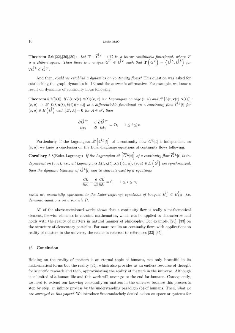
And then, could we establish a dynamics on continuity flows? This question was asked for
establishing the graph dynamics in [13] and the answer is affirmative. For example, we know a
result on dynamics of continuity flows following.
Theorem 5.7([30]) If L(t,x(t), x(t))(v, u) is a Lagrangian on edge (v, u) and L [L(t,x(t), x(t))] :
(v, u) → L [L(t,x(t), x(t))(v, u)] is a differentiable functional on a continuity flow−→GL[t] for
(v, u) ∈ E(−→G)
with [L , A] = 0 for A ∈ A , then
∂−→GL
∂xi− d
dt
∂−→GL
∂xi= O, 1 ≤ i ≤ n.
Particularly, if the Lagrangian L[−→GL[t]
]of a continuity flow
−→GL[t] is independent on
(v, u), we know a conclusion on the Euler-Lagrange equations of continuity flows following.
Corollary 5.8(Euler-Lagrange) If the Lagrangian L[−→GL[t]
]of a continuity flow
−→GL[t] is in-
dependent on (v, u), i.e., all Lagrangians L(t,x(t), x(t))(v, u), (v, u) ∈ E(−→G)
are synchronized,
then the dynamic behavior of−→GL[t] can be characterized by n equations
∂L
∂xi− d
dt
∂L
∂xi= 0, 1 ≤ i ≤ n,
which are essentially equivalent to the Euler-Lagrange equations of bouquet−→BL
1 ∈−→B1B, i.e,
dynamic equations on a particle P .
All of the above-mentioned works shows that a continuity flow is really a mathematical
element, likewise elements in classical mathematics, which can be applied to characterize and
holds with the reality of matters in natural manner of philosophy. For example, [25], [33] on
the structure of elementary particles. For more results on continuity flows with applications to
reality of matters in the universe, the reader is refereed to references [22]-[35].
§6. Conclusion
Holding on the reality of matters is an eternal topic of humans, not only beautiful in its
mathematical forms but the reality [35], which also provides us an endless resource of thought
for scientific research and then, approximating the reality of matters in the universe. Although
it is limited of a human life and this work will never go to the end for humans. Consequently,
we need to extend our knowing constantly on matters in the universe because this process is
step by step, an infinite process by the understanding paradigm (6) of humans. Then, what we
are surveyed in this paper? We introduce Smarandachely denied axiom on space or systems for
Reality with Smarandachely Denied Axiom 17
the understanding matters because they are not homogenous or equal in the eyes of humans,
show its a generalized form equalizing to Smarandache multispace which is an appropriately
understanding of matters by philosophy and then, explain how to extend classical mathematics
to mathematical combinatorics by CC conjecture. All of the discussions firmly convince one
that Smarandachely denied axiom is an important axiom or notion for extending today’s science
which will further pushes humans to know the truth of matters in the universe, i.e., the reality.
References
[1] A.A.A.Agboola and B.Davvaz, Some properties of birings, International J. Math.Combin.,
Vol.2(2013), 24-33.
[2] Mustafa Altın and Zuhal Kucukarslan Yuzbası, Surfaces using Smarandache asymptotic
curves in Galilean space, International J. Math.Combin., Vol.3(2020), 1-15.
[3] S.Bhattacharya, A model to a Smarandache geometry, http://fs.unm.edu/ScienceLibrary/
Geometries.htm.
[4] G.Birkhoff and S.MacLane, A Survey of Modern Algebra (4th edition), Macmillan Publish-
ing Co., Inc, 1977.
[5] J.L.Groos and T.W.Tucker, Topological Graph Theory, John Wiley & Sons, 1987.
[6] Howard Iseri, Smarandache Manifolds, American Research Press, Rehoboth, NM,2002.
[7] Howard Iseri, Partially paradoxist Smarandache geometries, http://fs.unm.edu/ScienceLib-
rary/Geometries.htm.
[8] L.Kuciuk and M.Antholy, An introduction to Smarandache geometries, JP Journal of
Geometry & Topology, 5, 1(2005), 77-81.
[9] Tanju Kahraman and Hasan Huseyin Ugurlu, Smarandache curves of curves lying on light-
like cone in R31, International J. Math.Combin., Vol.1,3(2017), 1-9.
[10] Linfan Mao, A new view of combinatorial maps by Smarandache’s notion, in L.Mao ed.
Collected Papers on Mathematical Combinatorics(I), World Academic Union (World Aca-
demic Press), 2006.
[11] Linfan Mao, Geometrical theory on combinatorial manifolds, JP J. Geometry and Topology,
Vol.7, 1(2007), 65-113.
[12] Linfan Mao, An introduction to Smarandache multi-spaces and mathematical combina-
torics, Scientia Magna, Vol.3, 1(2007), 54-80.
[13] Lifan Mao, Combinatorial speculation and combinatorial conjecture for mathematics, Re-
ported at The 2th Conference on Combinatorics and Graph Theory of China, August 16-19,
2006, Tianjing, P.R.China, International J. Math.Combin., Vol.1,1(2007), 1-19.
[14] Linfan Mao, Combinatorial fields - An introduction, International J. Math.Combin., Vol.3
(2009),1-22.
[15] Linfan Mao, Relativity in Combinatorial Gravitational Fields, Progress in Physics, Vol.3,
2010, 39-50.
[16] Linfan Mao, Automorphism Groups of Maps, Surfaces and Smarandache Geometries (Sec-
ond edition), The Education Publisher Inc., USA, 2011.
18 Linfan MAO
[17] Linfan Mao, Smarandache Multi-Space Theory (2nd Edition), The Education Publisher
Inc., USA, 2011.
[18] Linfan Mao, Combinatorial Geometry with Applications to Field Theory (2nd Edition),
The Education Publisher Inc., USA, 2011.
[19] Linfan Mao, Non-solvable spaces of linear equation systems, International J. Math.Combin.,
Vol.2, 2012, 9-23.
[20] Linfan Mao, Global stability of non-solvable ordinary differential equations with applica-
tions, International J. Math.Combin., Vol.1, 2013, 1-37.
[21] Linfan Mao, Non-solvable equation systems with graphs embedded in Rn, Proceedings of
the First International Conferences on Smarandache Multispace & Multistructures, The
Education Publisher Inc., 2013.
[22] Linfan Mao, Mathematics on non-mathematics - A combinatorial contribution, Interna-
tional J.Math. Combin., Vol.3(2014), 1-34.
[22] Linfan Mao, Extended Banach−→G -flow spaces on differential equations with applications,
Electronic J.Mathematical Analysis and Applications, Vol.3, No.2 (2015), 59-91.
[24] Linfan Mao, Cauchy problem on non-solvable system of first order partial differential equa-
tions with applications, Methods and Applications of Analysis, Vol. 22, 2(2015), 171-200.
[25] Linfan Mao, A review on natural reality with physical equation, Progress in Physics, Vol.11,
3(2015), 276-282.
[26] Linfan Mao, Mathematics with natural reality – action flows, Bull.Cal.Math.Soc., Vol.107,
6(2015), 443-474.
[27] Linfan Mao, Mathematical combinatorics with natural reality, International J.Math. Com-
bin., Vol.2(2017), 11-33.
[28] Linfan Mao, Complex system with flows and synchronization, Bull.Cal.Math.Soc., Vol.109,
6(2017), 461-484.
[29] Linfan Mao, Mathematical 4th crisis: to reality, International J.Math. Combin., Vol.3(2018),
147-158.
[30] Linfan Mao, Harmonic flow’s dynamics on animals in microscopic level with balance re-
covery, International J.Math. Combin., Vol.1(2019), 1-44.
[31] Linfan Mao, Science’s dilemma – A review on science with applications, Progress in Physics,
Vol.15, 2(2019), 78–85.
[32] Linfan Mao, Graphs, Networks and Natural Reality– from Intuitive Abstracting to Theory,
International J.Math. Combin., Vol.4(2019), 1-18.
[33] Linfan Mao, Mathematical elements on natural reality, Bull. Cal. Math. Soc., 111, 6(2019),
597C618.
[34] Linfan Mao, Dynamic network with e-index applications, International J.Math. Combin.,
Vol.4(2020), 1-35.
[35] Linfan Mao, Reality or mathematical formality – Einstein’s general relativity on multi-
fields, Chinese J.Mathmatical Science, Vol.1, 1(2021), 1-16.
[36] Mahmut Mak and Hasan Altınbas, Spacelike Smarandache curves of timelike curves in anti
de Sitter 3-space, International J.Math. Combin., Vol.3(2016), 1-16.
[37] F.Smarandache, Paradoxist Geometry, State Archives from Valcea, Rm. Valcea, Romania,
Reality with Smarandachely Denied Axiom 19
1969, and in Paradoxist Mathematics, Collected Papers (Vol. II), Kishinev University
Press, Kishinev, 5-28, 1997.
[38] F.Smarandache, A Unifying Field in Logics, Neutrosophic Logic, Neutrosophy, Neutrosoph-
ic Set, Neutrosophic Probability, American Research Press, 1998.
[39] F.Smarandache, A new form of matter – unmatter, composed of particles and anti-particles,
Progess in Physics, Vol.1(2005), 9-11.
[40] F.Smarandache, S-denying a theory, International J.Math.Combin., Vol.2(2013), 1-7.
[41] F.Smarandache, Degree of negation of an axiom, http://fs.unm.edu/ScienceLibrary/Geom-
etries.htm.
[42] E.M.Solouma and M. M. Wageeda, Special Smarandache curves according to bishop frame
in Euclidean spacetime, International J.Math. Combin., Vol.1(2017), 1-9.
[43] Melih Turgut, Smarandache breadth pseudo null curves in minkowski space-time, Interna-
tional J.Math. Combin., Vol.1(2009), 46-49.
[44] Melih Turgut and Suha Yilmaz, Smarandache curves in minkowski space-time, Interna-
tional J.Math. Combin., Vol.3(2008), 51-55.
[45] Suha Yılmaz and Umit Ziya Savcı, Smarandache curves and applications according to
type-2 bishop frame in Euclidean 3-space, International J.Math. Combin., Vol.1(2016),
1-15.
[46] Suleyman Senyurt, Abdussamet Calıskan, Unzile Celik, N∗C∗ Smarandache curve of Ber-
trand curves pair according to Frenet frame, International J.Math. Combin., Vol.1(2016),
1-7.
[47] M.Tegmark, Parallel universes, in Science and Ultimate Reality: From Quantum to Cos-
mos, ed. by J.D.Barrow, P.C.W.Davies and C.L.Harper, Cambridge University Press,
2003.
[48]] W.B.Vasantha Kandasamy, Bialgebraic Structures and Smarandache Bialgebraic Struc-
tures, American Research Press, 2003.
[49] W.B.Vasantha Kandasamy and F.Smarandache, N-Algebraic Structures and S-N-Algebraic
Structures, HEXIS, Phoenix, Arizona, 2005.
[50] YasinUnluturk, Suha Yılmaz, Smarandache curves of a spacelike curve according to the
bishop frame of type-2, International J.Math. Combin., Vol.4(2016), 21-28.
International J.Math. Combin. Vol.3(2021), 20-31
A New Characterization of
Ruled Surfaces According to q-Frame Vectors in Euclidean 3-Space
Cumali Ekici1, Gul Ugur Kaymanlı2, Seda Okur1
1. Department of Mathematics and Computer Science, Eskisehir Osmangazi University, Eskisehir, Turkey
2. Department of Mathematics, Cankırı Karatekin University, Cankırı, Turkey
E-mail: [email protected], [email protected], [email protected]
Abstract: In this work, we study new families of ruled surfaces generated by q- frame
vectors called quasi vectors in 3-dimensional Euclidean space. First, the characterizations
of these ruled surfaces such as first and second fundamental forms, Gaussian and mean
curvatures are given. After we work on the ruled surfaces generated by the general vector
field and give the same caharacterizations for these surfaces whose director is general vector
field, we investigate some geometric properties such as developability, minimality, striction
curve, and distribution parameter. Lastly, we visualize the surfaces whose directors are
tangent, q-normal, q-binormal and general vector field by taking two different curves.
Key Words: Gaussian curvature, mean curvature, quasi frame, ruled surface.
AMS(2010): 53A05, 53A10, 57R25.
§1. Introduction
In order to understand what’s going on around us, we need to work on the surfaces. Therefore,
it is important to have an idea about how to construct the surfaces. Considering the structural
advantage of ruled surfaces and the ease of constructing their geometries, ruled surfaces are one
of the most attractive surfaces to work on. The ruled surface is a special type of surface which
is generated by the motion of a straight line (ruling) along a curve.
After these surfaces were found and investigated by Gaspard Mongea, Ravani and Ku
studied ruled surface and examined some properties of them in 1991. Some of the studies have
been done by Aydemir and Kasap in 2005, Sarioglugil and Tutar in 2007, Ali et. al. in 2013,
Senturk and Yuce in 2015, Unluturk et. al., in 2016, Dede et al. in 2017, Kaymanli in 2020
and Gozutok et al., in 2020 in Euclidean space [1], [4], [5], [7], [9], [12]-[14], [17] while Turgut
and Hacisalihoglu in 1998, Kimm and Yoon in 2004, Tosun and Gungor in 2005, Orbay and
Aydemir in 2019 and in 2010, Kaymanli et. al., in 2020 in Minkowski space [2], [8], [10], [11],
[15], [16].
In this work, we study new families of ruled surfaces generated by q- frame vectors called
quasi vectors in 3-dimensional Euclidean space. First, the characterizations of these ruled sur-
faces such as first and second fundamental forms, Gaussian and mean curvatures are given.
1Received June 3, 2021, Accepted August 28, 2021.
A New Characterization of Ruled Surfaces According to q-Frame Vectors in Euclidean 3-Space 21
After we work on the ruled surfaces generated by the general vector field and give the same
caharacterizations for these surfaces whose director is general vector field, we investigate some
geometric properties such as developability, minimality, striction curve, and distribution pa-
rameter. Lastly, we visualize the surfaces whose directors are tangent, q-normal, q-binormal
and general vector field by taking two different curves.
§2. Preliminaries
In this section, we give some background information about Frenet frame and how to construct
q-frame. Let α(s) be a space curve with a non-vanishing second derivative. The Frenet frame
is written as
t =α′
‖α′‖, b =
α′ ∧ α′′
‖α′ ∧ α′′‖, n = b ∧ t.
The curvature κ and the torsion τ are given by
κ =‖α′ ∧ α′′‖‖α′‖3
, τ =det(α′, α′′, α′′′)
‖α′ ∧ α′′‖2.
The well-known Frenet formulas are given byt′
n′
b′
= v
0 κ 0
−κ 0 τ
0 −τ 0
t
n
b
(1)
where v = ‖α′(s)‖ .
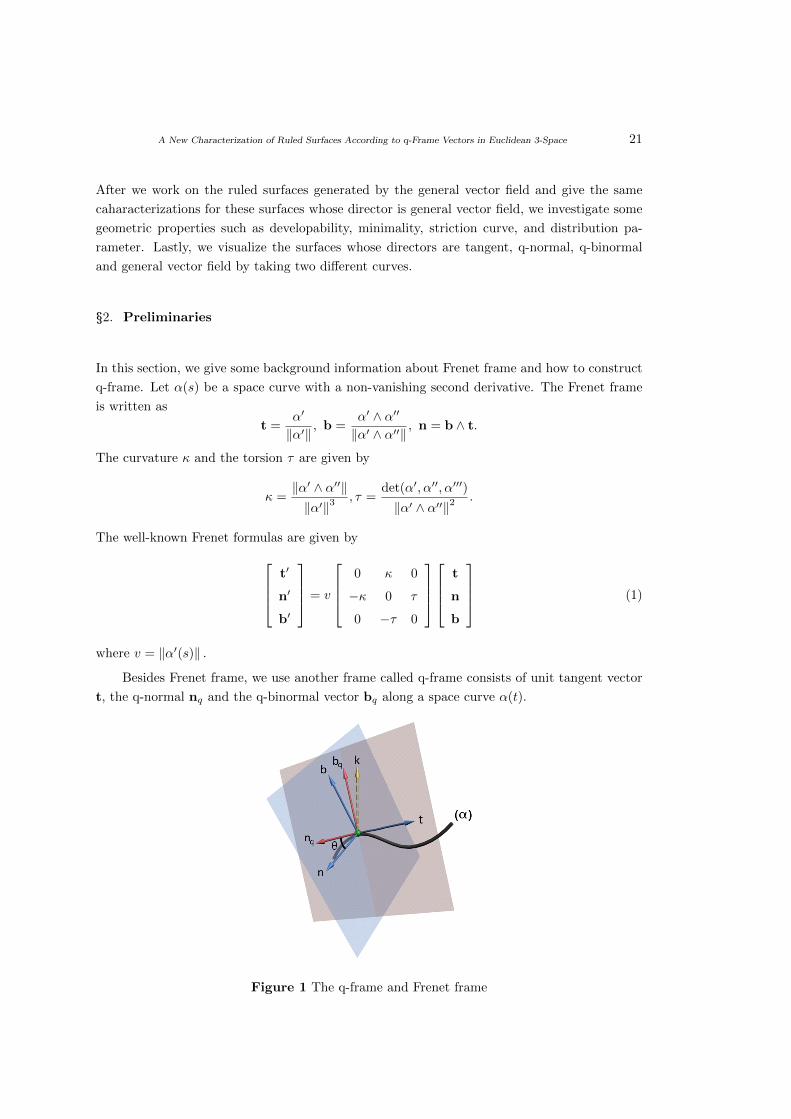
Besides Frenet frame, we use another frame called q-frame consists of unit tangent vector
t, the q-normal nq and the q-binormal vector bq along a space curve α(t).
Figure 1 The q-frame and Frenet frame
22 Cumali Ekici, Gul Ugur Kaymanlı and Seda Okur
The q-frame {t,nq,bq,k} is defined by
t =α′
‖α′‖,nq =
t ∧ k
‖t ∧ k‖,bq = t ∧ nq (2)
shown in Figure 1, where k is the projection vector [3].
Without loss of generality, we chose the projection vector k = (0, 0, 1) in this study. How-
ever, the q-frame is singular in all cases where t and k are parallel. Thus, in those cases where
t and k are parallel the projection vector k can be chosen as k = (0, 1, 0) or k = (1, 0, 0).
In order to define a relation between q-frame and Frenet frame, we pick Euclidean angle
θ between the principal normal n and q-normal nq vectors. Then the relation matrix may be
expressed as t
nq
bq
=
1 0 0
0 cos θ sin θ
0 − sin θ cos θ
t
n
b
(3)
or t
n
b
=
1 0 0
0 cos θ − sin θ
0 sin θ cos θ
t
nq
bq
. (4)
Let α(s) be a curve that is parameterized by arc length s. Differentiating (3) with respect
to s, then substituting (4) into the results gives the variation equations of the q-frame in the
following form t′
n′q
b′q
=
0 k1 k2
−k1 0 k3
−k2 −k3 0
t
nq
bq
, (5)
where the q-curvatures are
k1 = 〈t′,nq〉
k2 = 〈t′,bq〉
k3 =⟨n′q,bq
⟩.
(6)
The parametric equation of ruled surface ϕ(s, v) is given as
ϕ(s, v) = α(s) + vX(s), (7)
where α(s) is a curve and X(s) is a generator vector. The distribution parameter of the ruled
surface is identified by (see [6], [14])
PX =det(αs, X,Xs)
〈Xs, Xs〉. (8)
The striction point on the ruled surface is the foot of the common perpendicular line
A New Characterization of Ruled Surfaces According to q-Frame Vectors in Euclidean 3-Space 23
successive rulings on the main ruling. It is given as
βX(s) = α(s)− 〈αs, Xs〉〈Xs, Xs〉
X(s) (9)
Let M be a regular surface given with the parameterization ϕ(s, v) in E3. The tangent
space of M at an arbitrary point is spanned by the vectors ϕs and ϕv. The coefficients of the
first fundamental form of M are defined as
E = 〈ϕs, ϕs〉, F = 〈ϕs, ϕv〉, G = 〈ϕv, ϕv〉, (10)
where 〈, 〉 is the Euclidean inner product. Then the unit normal vector field of M is defined as
N =ϕs ∧ ϕv||ϕs ∧ ϕv||
. (11)
The coefficients of the second fundamental form of M are defined as
e = 〈ϕss, N〉, f = 〈ϕsv, N〉, g = 〈ϕvv, N〉. (12)
The Gaussian curvature and the mean curvature of M are given by
K =eg − f2
EG− F 2(13)
and
H =Eg +Ge− 2Ff
2(EG− F 2), (14)
respectively.
Theorem 2.1([12]) The ruled surface is developable if and only if PX = 0 .
Theorem 2.2 The ruled surface is minimal if and only if H = 0.
§3. Ruled Surfaces Generated by q-Frame Vectors
The ruled surfaces generated by q-frame vectors t, nq, bq are given as
φt(s, v) = α(s) + vt(s),
φnq (s, u) = α(s) + unq(s),
φbq (s, z) = α(s) + zbq(s),
respectively. The ruled surface generated by general vector filed X is written as
φX(s, w) = α(s) + wX(s) (15)
24 Cumali Ekici, Gul Ugur Kaymanlı and Seda Okur
where X(s) = x1(s)t+ x2(s)nq + x3(s)bq.
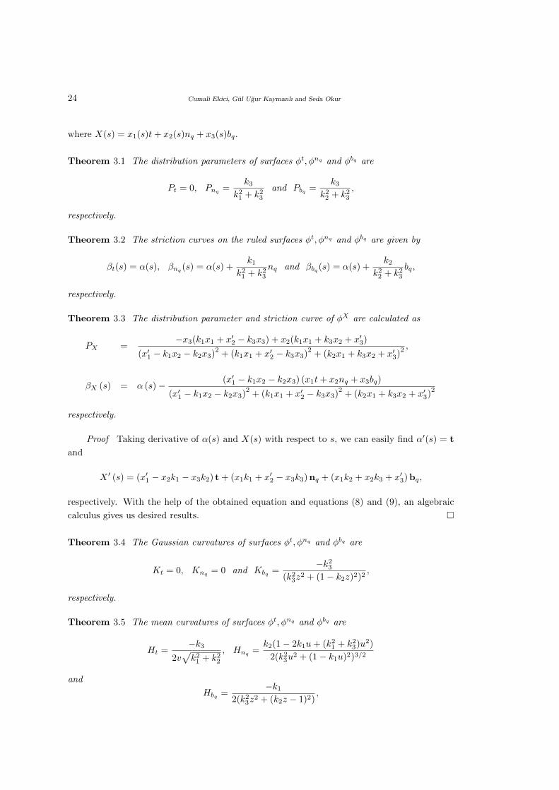
Theorem 3.1 The distribution parameters of surfaces φt, φnq and φbq are
Pt = 0, Pnq=
k3
k21 + k2
3
and Pbq =k3
k22 + k2
3
,
respectively.
Theorem 3.2 The striction curves on the ruled surfaces φt, φnq and φbq are given by
βt(s) = α(s), βnq(s) = α(s) +
k1
k21 + k2
3
nq and βbq (s) = α(s) +k2
k22 + k2
3
bq,
respectively.
Theorem 3.3 The distribution parameter and striction curve of φX are calculated as
PX =−x3(k1x1 + x′2 − k3x3) + x2(k1x1 + k3x2 + x′3)
(x′1 − k1x2 − k2x3)2
+ (k1x1 + x′2 − k3x3)2
+ (k2x1 + k3x2 + x′3)2 ,
βX (s) = α (s)− (x′1 − k1x2 − k2x3) (x1t+ x2nq + x3bq)
(x′1 − k1x2 − k2x3)2
+ (k1x1 + x′2 − k3x3)2
+ (k2x1 + k3x2 + x′3)2
respectively.
Proof Taking derivative of α(s) and X(s) with respect to s, we can easily find α′(s) = t
and
X ′ (s) = (x′1 − x2k1 − x3k2) t + (x1k1 + x′2 − x3k3) nq + (x1k2 + x2k3 + x′3) bq,
respectively. With the help of the obtained equation and equations (8) and (9), an algebraic
calculus gives us desired results. �
Theorem 3.4 The Gaussian curvatures of surfaces φt, φnq and φbq are
Kt = 0, Knq = 0 and Kbq =−k2
3
(k23z
2 + (1− k2z)2)2,
respectively.
Theorem 3.5 The mean curvatures of surfaces φt, φnq and φbq are
Ht =−k3
2v√k2
1 + k22
, Hnq =k2(1− 2k1u+ (k2
1 + k23)u2)
2(k23u
2 + (1− k1u)2)3/2
and
Hbq =−k1
2(k23z
2 + (k2z − 1)2),
A New Characterization of Ruled Surfaces According to q-Frame Vectors in Euclidean 3-Space 25
respectively.
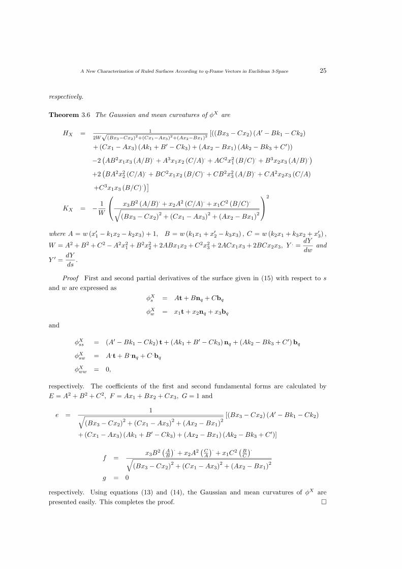
Theorem 3.6 The Gaussian and mean curvatures of φX are
HX = 1
2W√
(Bx3−Cx2)2+(Cx1−Ax3)2+(Ax2−Bx1)2[((Bx3 − Cx2) (A′ −Bk1 − Ck2)
+ (Cx1 −Ax3) (Ak1 +B′ − Ck3) + (Ax2 −Bx1) (Ak2 −Bk3 + C ′))
−2(AB2x1x3 (A/B)
.+A3x1x2 (C/A)
.+AC2x2
1 (B/C).+B3x2x3 (A/B)
.)+2(BA2x2
2 (C/A).+BC2x1x2 (B/C)
.+ CB2x2
3 (A/B).+ CA2x2x3 (C/A)
+C3x1x3 (B/C).)]
KX = − 1
W
x3B2 (A/B)
.+ x2A
2 (C/A).+ x1C
2 (B/C).√
(Bx3 − Cx2)2
+ (Cx1 −Ax3)2
+ (Ax2 −Bx1)2
2
where A = w (x′1 − k1x2 − k2x3) + 1, B = w (k1x1 + x′2 − k3x3) , C = w (k2x1 + k3x2 + x′3) ,
W = A2 +B2 +C2 −A2x21 +B2x2
2 + 2ABx1x2 +C2x23 + 2ACx1x3 + 2BCx2x3, Y
. =dY
dwand
Y ′ =dY
ds.
Proof First and second partial derivatives of the surface given in (15) with respect to s
and w are expressed as
φXs = At +Bnq + Cbq
φXw = x1t + x2nq + x3bq
and
φXss = (A′ −Bk1 − Ck2) t + (Ak1 +B′ − Ck3) nq + (Ak2 −Bk3 + C ′) bq
φXsw = A.t +B.nq + C .bq
φXww = 0,
respectively. The coefficients of the first and second fundamental forms are calculated by
E = A2 +B2 + C2, F = Ax1 +Bx2 + Cx3, G = 1 and
e =1√
(Bx3 − Cx2)2
+ (Cx1 −Ax3)2
+ (Ax2 −Bx1)2
[(Bx3 − Cx2) (A′ −Bk1 − Ck2)
+ (Cx1 −Ax3) (Ak1 +B′ − Ck3) + (Ax2 −Bx1) (Ak2 −Bk3 + C ′)]
f =x3B
2(AB
).+ x2A
2(CA
).+ x1C
2(BC
).√(Bx3 − Cx2)
2+ (Cx1 −Ax3)
2+ (Ax2 −Bx1)
2
g = 0
respectively. Using equations (13) and (14), the Gaussian and mean curvatures of φX are
presented easily. This completes the proof. �
26 Cumali Ekici, Gul Ugur Kaymanlı and Seda Okur
Corollary 3.7 The ruled surface φt is developable and the ruled surfaces φnq and φbq are
developable if and only if k3 = 0.
Corollary 3.8 The ruled surface φt is minimal if and only if k3 = 0, the ruled surface φbq is
minimal if and only if k1 = 0 and the ruled surface φnq is minimal if and only if either k2 = 0
or u =k1(1±
√1−k23)
k21+k23.
Corollary 3.9 There is a relation between Kbq , Hbq and Pbq as follows
Kbq
Hbq
=2k2
3
k1(k23z
2 + (1− k2z)
andKbq
Pbq=
−k3(k22 + k2
3)
(k23z
2 + (1− k2z)2)2.
§4. Examples
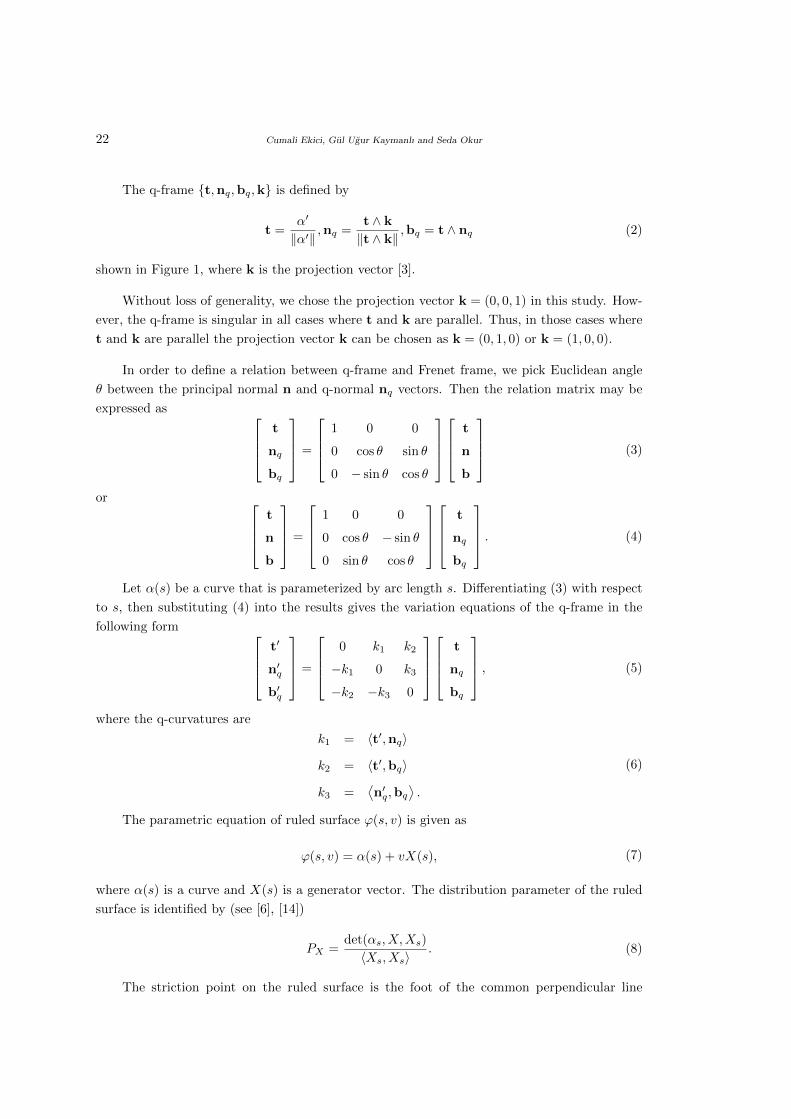
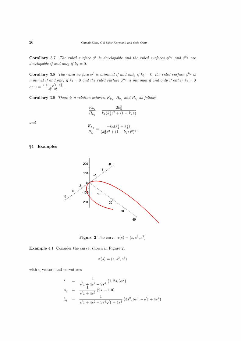
Figure 2 The curve α(s) = (s, s2, s3)
Example 4.1 Consider the curve, shown in Figure 2,
α(s) = (s, s2, s3)
with q-vectors and curvatures
t =1√
1 + 4s2 + 9s4
(1, 2s, 3s2
)nq =
1√1 + 4s2
(2s,−1, 0)
bq =1√
1 + 4s2 + 9s4√
1 + 4s2
(3s2, 6s3,−
√1 + 4s2
)
A New Characterization of Ruled Surfaces According to q-Frame Vectors in Euclidean 3-Space 27
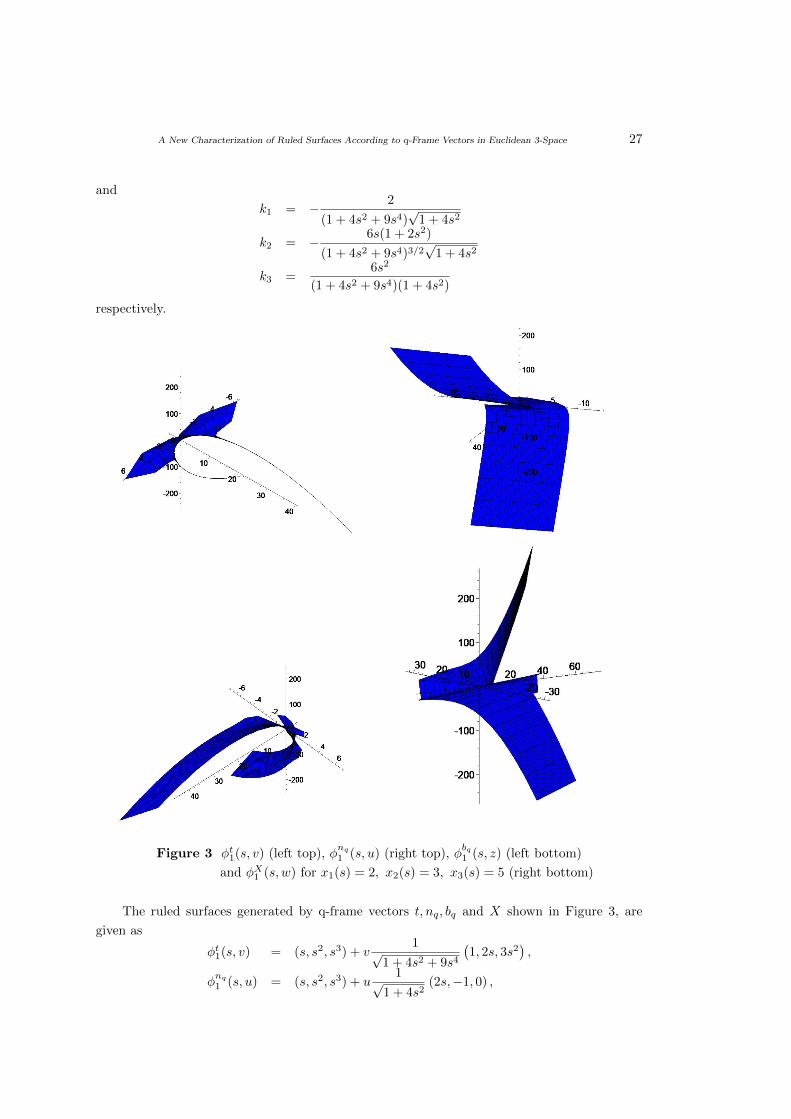
and
k1 = − 2
(1 + 4s2 + 9s4)√
1 + 4s2
k2 = − 6s(1 + 2s2)
(1 + 4s2 + 9s4)3/2√
1 + 4s2
k3 =6s2
(1 + 4s2 + 9s4)(1 + 4s2)
respectively.
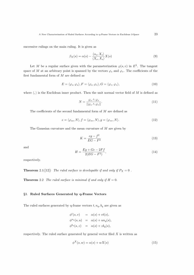
Figure 3 φt1(s, v) (left top), φnq
1 (s, u) (right top), φbq1 (s, z) (left bottom)
and φX1 (s, w) for x1(s) = 2, x2(s) = 3, x3(s) = 5 (right bottom)
The ruled surfaces generated by q-frame vectors t, nq, bq and X shown in Figure 3, are
given as
φt1(s, v) = (s, s2, s3) + v1√
1 + 4s2 + 9s4
(1, 2s, 3s2
),
φnq
1 (s, u) = (s, s2, s3) + u1√
1 + 4s2(2s,−1, 0) ,
28 Cumali Ekici, Gul Ugur Kaymanlı and Seda Okur
φbq1 (s, z) = (s, s2, s3) + z
1√1 + 4s2 + 9s4
√1 + 4s2
(3s2, 6s3,−
√1 + 4s2
),
and
φX1 (s, w) = (s, s2, s3) + w
(x1(s)(
1√1 + 4s2 + 9s4
(1, 2s, 3s2
))
+x2(s)(1√
1 + 4s2(2s,−1, 0))
+x3(s)(1√
1 + 4s2 + 9s4√
1 + 4s2
(3s2, 6s3,−
√1 + 4s2
))
),
respectively.
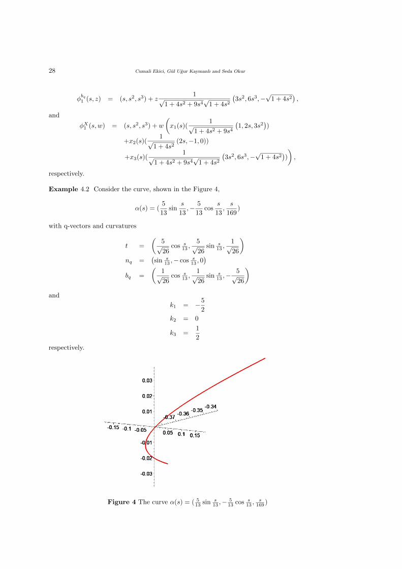
Example 4.2 Consider the curve, shown in the Figure 4,
α(s) = (5
13sin
s
13,− 5
13cos
s
13,s
169)
with q-vectors and curvatures
t =
(5√26
cos s13 ,
5√26
sin s13 ,
1√26
)nq =
(sin s
13 ,− cos s13 , 0
)bq =
(1√26
cos s13 ,
1√26
sin s13 ,−
5√26
)and
k1 = −5
2
k2 = 0
k3 =1
2
respectively.
Figure 4 The curve α(s) = ( 513 sin s
13 ,−513 cos s
13 ,s
169 )
A New Characterization of Ruled Surfaces According to q-Frame Vectors in Euclidean 3-Space 29
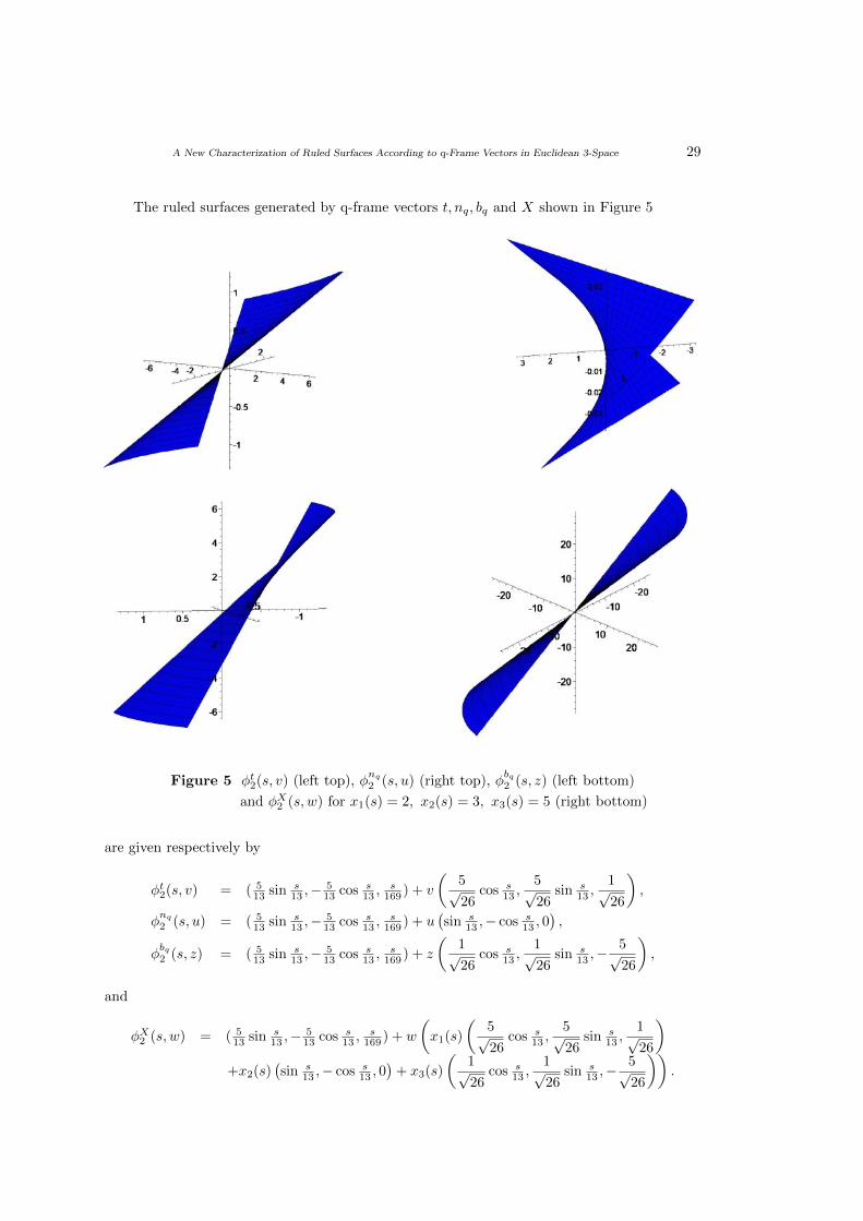
The ruled surfaces generated by q-frame vectors t, nq, bq and X shown in Figure 5
Figure 5 φt2(s, v) (left top), φnq
2 (s, u) (right top), φbq2 (s, z) (left bottom)
and φX2 (s, w) for x1(s) = 2, x2(s) = 3, x3(s) = 5 (right bottom)
are given respectively by
φt2(s, v) = ( 513 sin s
13 ,−513 cos s
13 ,s
169 ) + v
(5√26
cos s13 ,
5√26
sin s13 ,
1√26
),
φnq
2 (s, u) = ( 513 sin s
13 ,−513 cos s
13 ,s
169 ) + u(sin s
13 ,− cos s13 , 0
),
φbq2 (s, z) = ( 5
13 sin s13 ,−
513 cos s
13 ,s
169 ) + z
(1√26
cos s13 ,
1√26
sin s13 ,−
5√26
),
and
φX2 (s, w) = ( 513 sin s
13 ,−513 cos s
13 ,s
169 ) + w
(x1(s)
(5√26
cos s13 ,
5√26
sin s13 ,
1√26
)+x2(s)
(sin s
13 ,− cos s13 , 0
)+ x3(s)
(1√26
cos s13 ,
1√26
sin s13 ,−
5√26
)).
30 Cumali Ekici, Gul Ugur Kaymanlı and Seda Okur
For x1(s) = 2, x2(s) = 3, x3(s) = 5, the Gaussian curvature, mean curvature, distribution
parameter and striction curve of the surface φX2 (s, w), generated by X are calculated as
KX = − 7056
(68 + 1140w + 8721w2)2,
HX =
√1228(1228 + 26220w + 200583w2)
4√
884 + 14820w + 113373w2(68 + 1140w + 8721w2),
PX = − 56
153
βX(s) =
(125
663sin
s
13− 25
√26
663cos
s
13,−125
663cos
s
13− 25
√26
663sin
s
13,s
169+
115√
26
1989
),
respectively.
Acknowledgement
The first version of this manuscript, derived from the thesis written in Eskisehir Osmanga-
zi University, was presented in IV. International Scientific And Vocational Studies Congress
(BILMES 2019). All figures in this study were created by using maple programme.
References
[1] Ali A.T., Aziz H.S.A., Sorour A.H., Ruled surfaces generated by some special curves in
Euclidean 3-space, Journal of the Egyptian Mathematical Society, 2013; 21 (3): 285-294.
[2] Aydemir, I. and Orbay, K., The ruled surfaces generated by Frenet vectors of timelike ruled
surface in the Minkowski space R31, World Applied Science Journal, 6(5), 692-696, 2009.
[3] Dede, M., Ekici, C. and Gorgulu, A., Directional q-frame along a space curve, IJARCSSE,
5(12), 775-780, 2015.
[4] Dede, M., Tozak, H. and Ekici, C., On the parallel ruled surface with B-Darboux frame,
AHA, 106, 2017.
[5] Gozutok, U., Coban, H.A. and Sariroglu, Y., Ruled surfaces obtained by bending of curves,
Turkish Journal of Mathematics, 44: 300-306, 2020.
[6] Gray, A., Salamon, S. and Abbena, E., Modern Differential Geometry of Curves and Sur-
faces with Mathematica, Chapman and Hall/CRC, 2006.
[7] Kaymanli, G.U., Characterization of the evolute offset of ruled surfaces with B-Darboux
frame, Journal of New Theory, (33): 50-55, 2020.
[8] Kaymanli, G.U. Ekici, C. and Dede, M., Directional evolution of the ruled surfaces via the
evolution of their directrix using q-frame along a timelike space curve, European Journal
of Science and Technology, 20, 392-396, 2020.
[9] Kaymanlı, G.U. Ekici C. and Dede M., Bertrand offsets of ruled surface with B-Darboux
frame (Submitted).
[10] Kim Y.H., Yoon D.W., Classificiation of ruled surfaces in Minkowski 3-spaces, Journal of
Geometry and Physics, 49, 89-100, 2004.
A New Characterization of Ruled Surfaces According to q-Frame Vectors in Euclidean 3-Space 31
[11] Orbay, K. and Aydemir, I., The ruled surfaces generated by Frenet vectors of a curve in
R31, C.B.U. Fen Bilimleri Dergisi, 6(2), 155-160, 2010.
[12] Ravani, B. and Ku, T.S., Bertrand offsets of ruled surface and developable surface, Computer-
Aided Design, 23(2), 145-152, 1991.
[13] Sarioglugil, A. and Tutar, A., On ruled surface in Euclidean space, Int. J. Contemp. Math.
Sci., 2(1): 1-11, 2007.
[14] Senturk, G.Y. and Yuce, S., Characteristic properties of the ruled surface with Darboux
frame in E3, Kuwait J. Sci., 42(2), 14-33, 2015.
[15] Tosun M., Gungor, M.A., A study on time-like complemantary ruled surfaces in the
Minkowski n-space, Iranian Journal of Science and Technology Transaction : A-Science,
29 A2, 325-323, 2005.
[16] Turgut A, Hacısalihoglu H.H., Timelike ruled surfaces in the Minkowski 3-space II, Turkish
J. Math., 22, 33-46, 1998.
[17] Unluturk, Y. Cimdiker, M. and Ekici. C., Characteristic properties of the parallel ruled
surfaces with Darboux frame in E3 space, Communication in Mathematical Modeling and
Applications, 1(1), 26-43, 2016.
32 K. Shivashankara and G. Vinay
International J.Math. Combin. Vol.3(2021), 32-34
On Sears’s Basic Hypergeometric Series Transformation Formula
K. Shivashankara and G. Vinay
(Department of Mathematics, Yuvaraja’s College, University of Mysore, Mysuru, 570005, India)
E-mail: [email protected], [email protected]
Abstract: In this paper, we provide an alternative simple proof to Sears’s 3ϕ2 transforma-
tion formula using Gauss summation formula.
Key Words: Basic hypergeometric series, transformation formula, Gauss summation.
AMS(2010): 33D15.
§1. Introduction
For any complex number a and for any q with |q| < 1, (a; q)∞ or simply (a)∞ is defined as
follows:
(a)∞ = (a; q)∞ =
∞∏n=0
(1− aqn).
For any integer n, we define (a; q)n or simply (a)n as
(a)n =(a)∞
(aqn)∞, (1.1)
provided the denominator is well defined. For any two integers m and n, the following holds
good
(a)n(aqn)m = (a)m(aqm)n. (1.2)
The basic hypergeometric series s+1ϕs is defined by
s+1ϕs
a1, a2, · · · , as+1
b1, b2, · · · , bs; z
:=
∞∑n=0
(a1)n (a2)n · · · (as+1)n(q)n (b1)n (b2)n · · · (bs)n
zn,
where a1, a2, · · · , as+1, b1, b2, · · · , bs are any complex numbers, except that (bj)n 6= 0, 1 ≤ j ≤s, 0 ≤ n ≤ ∞. This series converges for all z with |z| < 1.
In his paper [3], D. B. Sears deduced the following 3ϕ2 transformation formula
∞∑n=0
(a)n (b)n (c)n(d)n (e)n (q)n
(de
abc
)n=
(b)∞(deab
)∞
(debc
)∞
(d)∞ (e)∞(deabc
)∞
∞∑n=0
(db
)n
(eb
)n
(deabc
)n(
deab
)n
(debc
)n
(q)nbn, (1.3)
1Received June 19, 2021, Accepted August 28, 2021.
On Sears’s Basic Hypergeometric Series Transformation Formula 33
where,∣∣∣ dcabc ∣∣∣ < 1, |b| < 1, and |q| < 1. Sears deduced the above transformation by letting one
of the parameters in his 4ϕ3 transformation to infinity. This identity has been widely in areas
of special functions and number theory. See for instance [1] and [2]. In this paper, we give a
simple proof to (1.3) using q-analogous of Gauss summation formula. This proof seems to be
new in the literature. We close this section by recalling the q-analogous of Gauss summation
formula and prove (1.3) in Section 2 following.
∞∑m=0
(a)m (b)m(c)m (q)m
( cab
)m=
(ca
)∞
(cb
)∞
(c)∞(cab
)∞, | c
ab| < 1. (1.4)
§2. Proof of (1.3)
From (1.4), it follows that
(A)∞ (B)∞(C)∞
(ABC
)∞
=
∞∑n=0
(CA
)n
(CB
)n
(C)n (q)n
(AB
C
)n,
∣∣∣ABC
∣∣∣ < 1.
Taking A = dqm, B = eqm and C = deqm
b in the above, we obtain
(dqm)∞ (eqm)∞(deqm
b
)∞
(bqm)∞
=
∞∑n=0
(db
)n
(eb
)n
(q)n
(deqm
b
)n
(bqm)n. (2.1)
Using (1.1), we can write
∞∑m=0
(a)m (b)m (c)m(d)m (e)n (q)m
(de
abc
)m=
(b)∞(d)∞ (e)∞
∞∑m=0
(a)m (c)m
(deqm
b
)∞
(q)m
(de
abc
)m(dqm)∞ (eqm)∞(deqm
b
)∞
(bqm)∞
.
Using (2.1) in the above, we obtain
∞∑m=0
(a)m (b)m (c)m(d)m (e)n (q)m
(de
abc
)m=
(b)∞(deb
)∞
(d)∞ (e)∞
∞∑m=0
(a)m (c)m(q)m
(deb
)m
(de
abc
)m ∞∑n=0
(db
)n
(eb
)n
(q)n
(deqm
b
)n
(bqm)n.
Interchanging the order of summation in the above and using (1.2), we obtain
∞∑m=0
(a)m (b)m (c)m(d)m (e)m (q)m
(de
abc
)m=
(b)∞(deb
)∞
(d)∞ (e)∞
∞∑n=0
(db
)n
(eb
)n
(q)n(deb
)n
(b)n∞∑m=0
(a)m (c)m
(q)m
(deqn
b
)m
(deqn
abc
)m.
Now applying (1.4) to the inner series on the right hand side, we obtain
∞∑m=0
(a)m (b)m (c)m(d)m (e)n (q)m
(de
abc
)m=
(b)∞(deb
)∞
(d)∞ (e)∞
∞∑n=0
(db
)n
(eb
)n
(q)n(deb
)n
(b)n
(deqn
ab
)∞
(deqn
bc
)∞(
deqn
b
)∞
(deqn
abc
)∞
.
34 K. Shivashankara and G. Vinay
Notice that the equation (1.3) follows directly from the above on using (1.1). This completes
the proof. �
References
[1] G. E. Andrews and B. C. Berndt, Ramanujan’s Lost Notebook, Part II, Springer, 2009.
[2] G. Gaspar and M. Rahman, Basic Hypergeometric Series, 2nd edition, Cambridge Univer-
sity Press, Cambridge, 2004.
[3] Sears, D. B.,On the transformation theory of hypergeometric functions and cognate trigono-
metrical series, Proc. London Math. Soc. (2), 53, (1951), 158-180.
International J.Math. Combin. Vol.3(2021), 35-48
On Laplacian of Product of Randic and Sum-Connectivity
Energy of Graphs
R.Poojitha and Dr.Puttaswamy
(Department of Mathematics, P.E.S. college of Engineering, Mandya-571401, India)
E-mail: [email protected], [email protected]
Abstract: In this paper, we define the Laplacian of product of Randic and sum-connectivity
energy of a graph. Then, we compute the Laplacian of product of Randic and sum-
connectivity energies of complete graph, star graph, complete bipartite graph, the crown
graph, the (Sm ∧ P2) graph.
Key Words: Laplacian matrix, Laplacian of product of Randic and sum-connectivity
energy, graph.
AMS(2010): 05C50.
§1. Introduction
In [6] we define product of Randic and sum-connectivity energy of a simple graph G as follows:
Let a and b be two nonnegative real number with a 6= 0. The product of Randic and
sum-connectivity adjacency matrix of G is the n× n matrix Aprs = (aij) where
aij =
0, if i = j,
1√1
a(di+dj)b(didj)
, if the vertices vi and vj are adjacent,
0, if the vertices vi and vj are not adjacent.
The eigenvalues of the graph G are the eigenvalues of Aprs. Since Aprs is real and sym-
metric, its eigenvalues are real numbers which are denoted by λ1, λ2, λ3, · · · , λn, where
λ1 ≥ λ2 ≥ λ3 ≥ · · · ≥ λn.
Then the product of Randic and sum-connectivity energy of G is defined as
Eprs(G) =
n∑i=1
| λi | .
1Received August 5, 2021, Accepted August 30, 2021.
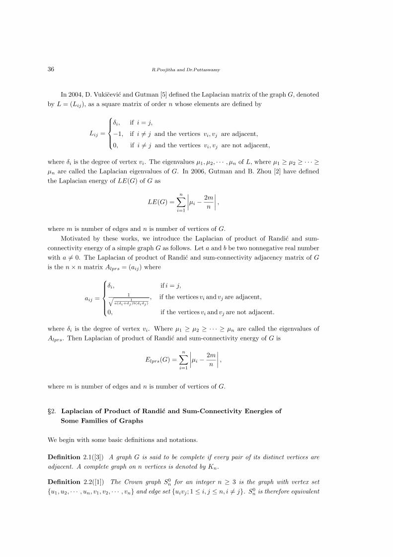
36 R.Poojitha and Dr.Puttaswamy
In 2004, D. Vukicevic and Gutman [5] defined the Laplacian matrix of the graph G, denoted
by L = (Lij), as a square matrix of order n whose elements are defined by
Lij =
δi, if i = j,
−1, if i 6= j and the vertices vi, vj are adjacent,
0, if i 6= j and the vertices vi, vj are not adjacent,
where δi is the degree of vertex vi. The eigenvalues µ1, µ2, · · · , µn of L, where µ1 ≥ µ2 ≥ · · · ≥µn are called the Laplacian eigenvalues of G. In 2006, Gutman and B. Zhou [2] have defined
the Laplacian energy of LE(G) of G as
LE(G) =
n∑i=1
∣∣∣∣µi − 2m
n
∣∣∣∣ ,where m is number of edges and n is number of vertices of G.
Motivated by these works, we introduce the Laplacian of product of Randic and sum-
connectivity energy of a simple graph G as follows. Let a and b be two nonnegative real number
with a 6= 0. The Laplacian of product of Randic and sum-connectivity adjacency matrix of G
is the n× n matrix Alprs = (aij) where
aij =
δi, if i = j,
1√1
a(di+dj)b(didj)
, if the vertices vi and vj are adjacent,
0, if the vertices vi and vj are not adjacent.
where δi is the degree of vertex vi. Where µ1 ≥ µ2 ≥ · · · ≥ µn are called the eigenvalues of
Alprs. Then Laplacian of product of Randic and sum-connectivity energy of G is
Elprs(G) =
n∑i=1
∣∣∣∣µi − 2m
n
∣∣∣∣ ,where m is number of edges and n is number of vertices of G.
§2. Laplacian of Product of Randic and Sum-Connectivity Energies of
Some Families of Graphs
We begin with some basic definitions and notations.
Definition 2.1([3]) A graph G is said to be complete if every pair of its distinct vertices are
adjacent. A complete graph on n vertices is denoted by Kn.
Definition 2.2([1]) The Crown graph S0n for an integer n ≥ 3 is the graph with vertex set
{u1, u2, · · · , un, v1, v2, · · · , vn} and edge set {uivj ; 1 ≤ i, j ≤ n, i 6= j}. S0n is therefore equivalent
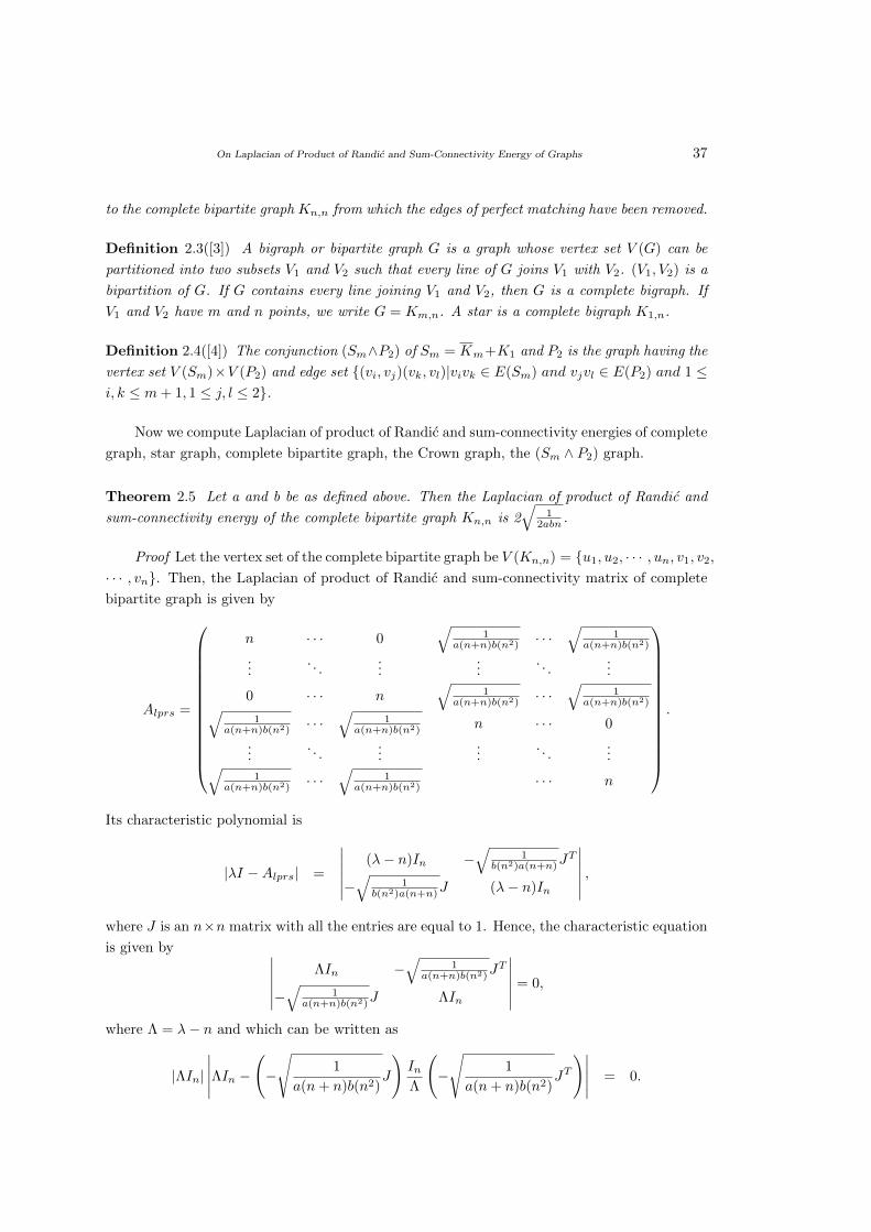
On Laplacian of Product of Randic and Sum-Connectivity Energy of Graphs 37
to the complete bipartite graph Kn,n from which the edges of perfect matching have been removed.
Definition 2.3([3]) A bigraph or bipartite graph G is a graph whose vertex set V (G) can be
partitioned into two subsets V1 and V2 such that every line of G joins V1 with V2. (V1, V2) is a
bipartition of G. If G contains every line joining V1 and V2, then G is a complete bigraph. If
V1 and V2 have m and n points, we write G = Km,n. A star is a complete bigraph K1,n.
Definition 2.4([4]) The conjunction (Sm∧P2) of Sm = Km+K1 and P2 is the graph having the
vertex set V (Sm)×V (P2) and edge set {(vi, vj)(vk, vl)|vivk ∈ E(Sm) and vjvl ∈ E(P2) and 1 ≤i, k ≤ m+ 1, 1 ≤ j, l ≤ 2}.
Now we compute Laplacian of product of Randic and sum-connectivity energies of complete
graph, star graph, complete bipartite graph, the Crown graph, the (Sm ∧ P2) graph.
Theorem 2.5 Let a and b be as defined above. Then the Laplacian of product of Randic and
sum-connectivity energy of the complete bipartite graph Kn,n is 2√
12abn .
Proof Let the vertex set of the complete bipartite graph be V (Kn,n) = {u1, u2, · · · , un, v1, v2,
· · · , vn}. Then, the Laplacian of product of Randic and sum-connectivity matrix of complete
bipartite graph is given by
Alprs =
n · · · 0√
1a(n+n)b(n2) · · ·
√1
a(n+n)b(n2)
.... . .
......
. . ....
0 · · · n√
1a(n+n)b(n2) · · ·
√1
a(n+n)b(n2)√1
a(n+n)b(n2) · · ·√
1a(n+n)b(n2) n · · · 0
.... . .
......
. . ....√
1a(n+n)b(n2) · · ·
√1
a(n+n)b(n2) · · · n
.
Its characteristic polynomial is
|λI −Alprs| =
∣∣∣∣∣∣(λ− n)In −
√1
b(n2)a(n+n)JT
−√
1b(n2)a(n+n)J (λ− n)In
∣∣∣∣∣∣ ,where J is an n×n matrix with all the entries are equal to 1. Hence, the characteristic equation
is given by ∣∣∣∣∣∣ΛIn −
√1
a(n+n)b(n2)JT
−√
1a(n+n)b(n2)J ΛIn
∣∣∣∣∣∣ = 0,
where Λ = λ− n and which can be written as
|ΛIn|
∣∣∣∣∣ΛIn −(−
√1
a(n+ n)b(n2)J
)InΛ
(−
√1
a(n+ n)b(n2)JT
)∣∣∣∣∣ = 0.
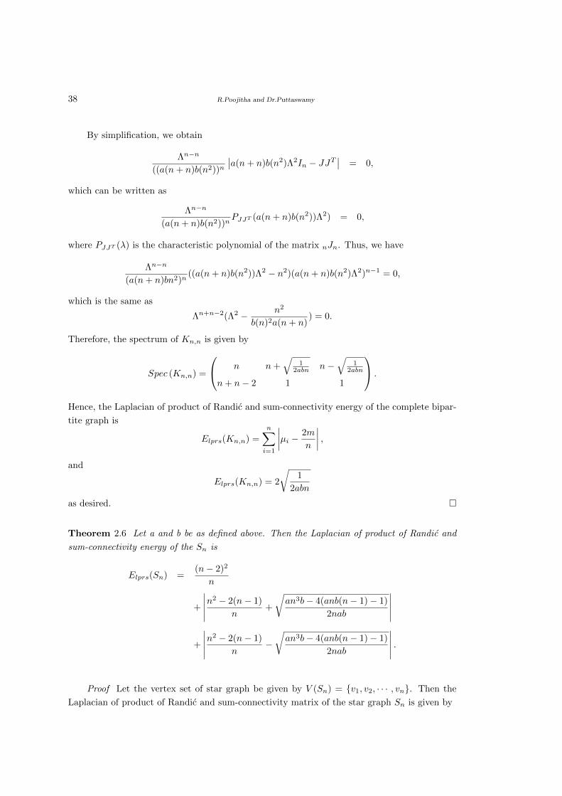
38 R.Poojitha and Dr.Puttaswamy
By simplification, we obtain
Λn−n
((a(n+ n)b(n2))n∣∣a(n+ n)b(n2)Λ2In − JJT
∣∣ = 0,
which can be written as
Λn−n
(a(n+ n)b(n2))nPJJT (a(n+ n)b(n2))Λ2) = 0,
where PJJT (λ) is the characteristic polynomial of the matrix nJn. Thus, we have
Λn−n
(a(n+ n)bn2)n((a(n+ n)b(n2))Λ2 − n2)(a(n+ n)b(n2)Λ2)n−1 = 0,
which is the same as
Λn+n−2(Λ2 − n2
b(n)2a(n+ n)) = 0.
Therefore, the spectrum of Kn,n is given by
Spec (Kn,n) =
n n+√
12abn n−
√1
2abn
n+ n− 2 1 1
.
Hence, the Laplacian of product of Randic and sum-connectivity energy of the complete bipar-
tite graph is
Elprs(Kn,n) =
n∑i=1
∣∣∣∣µi − 2m
n
∣∣∣∣ ,and
Elprs(Kn,n) = 2
√1
2abn
as desired. �
Theorem 2.6 Let a and b be as defined above. Then the Laplacian of product of Randic and
sum-connectivity energy of the Sn is
Elprs(Sn) =(n− 2)2
n
+
∣∣∣∣∣n2 − 2(n− 1)
n+
√an3b− 4(anb(n− 1)− 1)
2nab
∣∣∣∣∣+
∣∣∣∣∣n2 − 2(n− 1)
n−√an3b− 4(anb(n− 1)− 1)
2nab
∣∣∣∣∣ .
Proof Let the vertex set of star graph be given by V (Sn) = {v1, v2, · · · , vn}. Then the
Laplacian of product of Randic and sum-connectivity matrix of the star graph Sn is given by
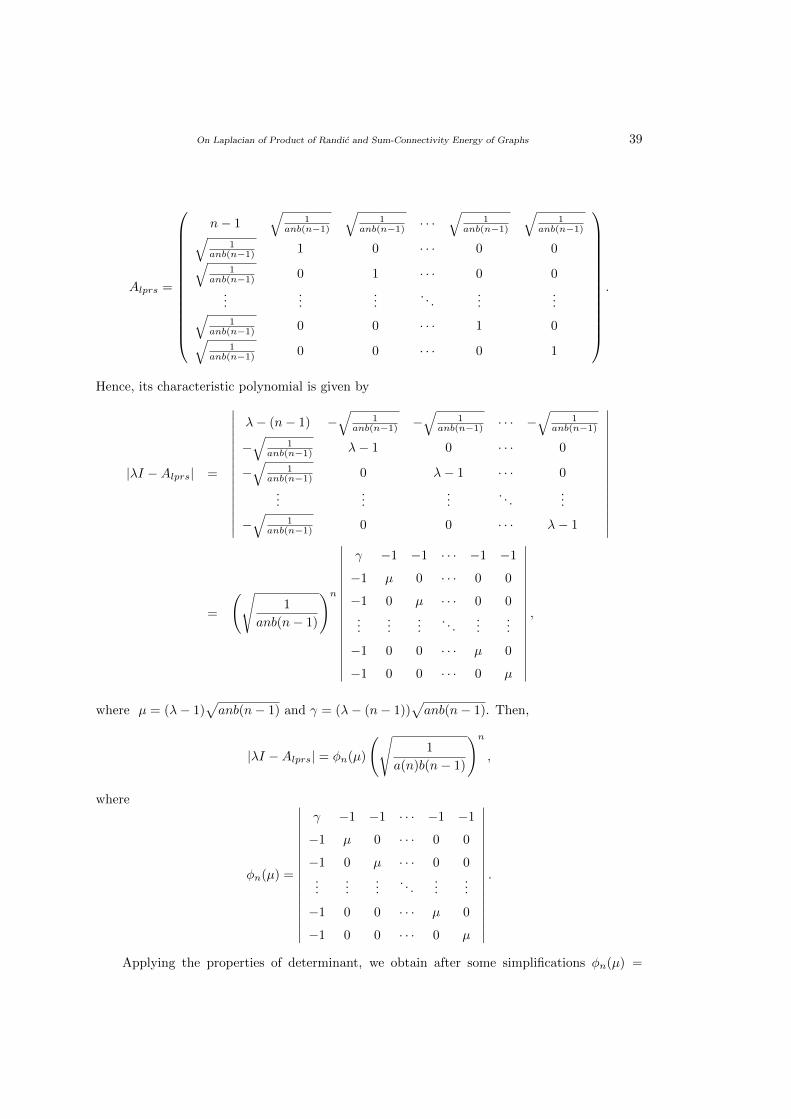
On Laplacian of Product of Randic and Sum-Connectivity Energy of Graphs 39
Alprs =
n− 1√
1anb(n−1)
√1
anb(n−1) · · ·√
1anb(n−1)
√1
anb(n−1)√1
anb(n−1) 1 0 · · · 0 0√1
anb(n−1) 0 1 · · · 0 0
......
.... . .
......√
1anb(n−1) 0 0 · · · 1 0√
1anb(n−1) 0 0 · · · 0 1
.
Hence, its characteristic polynomial is given by
|λI −Alprs| =
∣∣∣∣∣∣∣∣∣∣∣∣∣∣∣∣
λ− (n− 1) −√
1anb(n−1) −
√1
anb(n−1) · · · −√
1anb(n−1)
−√
1anb(n−1) λ− 1 0 · · · 0
−√
1anb(n−1) 0 λ− 1 · · · 0
......
.... . .
...
−√
1anb(n−1) 0 0 · · · λ− 1
∣∣∣∣∣∣∣∣∣∣∣∣∣∣∣∣
=
(√1
anb(n− 1)
)n∣∣∣∣∣∣∣∣∣∣∣∣∣∣∣∣∣
γ −1 −1 · · · −1 −1
−1 µ 0 · · · 0 0
−1 0 µ · · · 0 0...
......
. . ....
...
−1 0 0 · · · µ 0
−1 0 0 · · · 0 µ
∣∣∣∣∣∣∣∣∣∣∣∣∣∣∣∣∣,
where µ = (λ− 1)√anb(n− 1) and γ = (λ− (n− 1))
√anb(n− 1). Then,
|λI −Alprs| = φn(µ)
(√1
a(n)b(n− 1)
)n,
where
φn(µ) =
∣∣∣∣∣∣∣∣∣∣∣∣∣∣∣∣∣
γ −1 −1 · · · −1 −1
−1 µ 0 · · · 0 0
−1 0 µ · · · 0 0...
......
. . ....
...
−1 0 0 · · · µ 0
−1 0 0 · · · 0 µ
∣∣∣∣∣∣∣∣∣∣∣∣∣∣∣∣∣.
Applying the properties of determinant, we obtain after some simplifications φn(µ) =
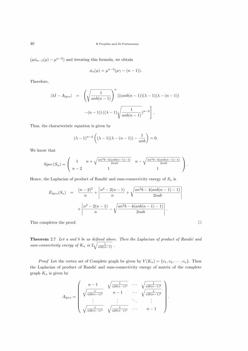
40 R.Poojitha and Dr.Puttaswamy
(µφn−1(µ)− µn−2) and iterating this formula, we obtain
φn(µ) = µn−2(µγ − (n− 1)).
Therefore,
|λI −Alprs| =
(√1
anb(n− 1)
)n[((anb(n− 1))(λ− 1)(λ− (n− 1))
−(n− 1)) ((λ− 1)
√1
anb(n− 1))n−2
].
Thus, the characteristic equation is given by
(λ− 1)n−2
((λ− 1)(λ− (n− 1))− 1
anb
)= 0.
We know that
Spec (Sn) =
1 n+√
an3b−4(anb(n−1)−1)2nab n−
√an3b−4(anb(n−1)−1)
2nab
n− 2 1 1
.
Hence, the Laplacian of product of Randic and sum-connectivity energy of Sn is
Elprs(Sn) =(n− 2)2
n+
∣∣∣∣∣n2 − 2(n− 1)
n+
√an3b− 4(anb(n− 1)− 1)
2nab
∣∣∣∣∣+
∣∣∣∣∣n2 − 2(n− 1)
n−√an3b− 4(anb(n− 1)− 1)
2nab
∣∣∣∣∣ .This completes the proof. �
Theorem 2.7 Let a and b be as defined above. Then the Laplacian of product of Randic and
sum-connectivity energy of Kn is 2√
1a2b(n−1) .
Proof Let the vertex set of Complete graph be given by V (Kn) = {v1, v2, · · · , vn}. Then
the Laplacian of product of Randic and sum-connectivity energy of matrix of the complete
graph Kn is given by
Alprs =
n− 1√
1a2b(n−1)3 · · ·
√1
a2b(n−1)3√1
a2b(n−1)3 n− 1 · · ·√
1a2b(n−1)3
......
. . ....√
1a2b(n−1)3
√1
a2b(n−1)3 · · · n− 1
.
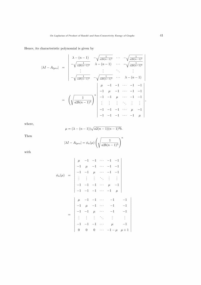
On Laplacian of Product of Randic and Sum-Connectivity Energy of Graphs 41
Hence, its characteristic polynomial is given by
|λI −Alprs| =
∣∣∣∣∣∣∣∣∣∣∣∣∣
λ− (n− 1) −√
1a2b(n−1)3 · · · −
√1
a2b(n−1)3
−√
1a2b(n−1)3 λ− (n− 1) · · · −
√1
a2b(n−1)3
......
. . ....
−√
1a2b(n−1)3 −
√1
a2b(n−1)3 · · · λ− (n− 1)
∣∣∣∣∣∣∣∣∣∣∣∣∣
=
(√1
a2b(n− 1)3
)n∣∣∣∣∣∣∣∣∣∣∣∣∣∣∣∣∣
µ −1 −1 · · · −1 −1
−1 µ −1 · · · −1 −1
−1 −1 µ · · · −1 −1...
......
. . ....
...
−1 −1 −1 · · · µ −1
−1 −1 −1 · · · −1 µ
∣∣∣∣∣∣∣∣∣∣∣∣∣∣∣∣∣,
where,
µ = (λ− (n− 1))√a2(n− 1)(n− 1)2b.
Then
|λI −Alprs| = φn(µ)
(√1
a2b(n− 1)3
)nwith
φn(µ) =
∣∣∣∣∣∣∣∣∣∣∣∣∣∣∣∣∣
µ −1 −1 · · · −1 −1
−1 µ −1 · · · −1 −1
−1 −1 µ · · · −1 −1...
......
. . ....
...
−1 −1 −1 · · · µ −1
−1 −1 −1 · · · −1 µ
∣∣∣∣∣∣∣∣∣∣∣∣∣∣∣∣∣
=
∣∣∣∣∣∣∣∣∣∣∣∣∣∣∣∣∣
µ −1 −1 · · · −1 −1
−1 µ −1 · · · −1 −1
−1 −1 µ · · · −1 −1...
......
. . ....
...
−1 −1 −1 · · · µ −1
0 0 0 · · · −1− µ µ+ 1
∣∣∣∣∣∣∣∣∣∣∣∣∣∣∣∣∣
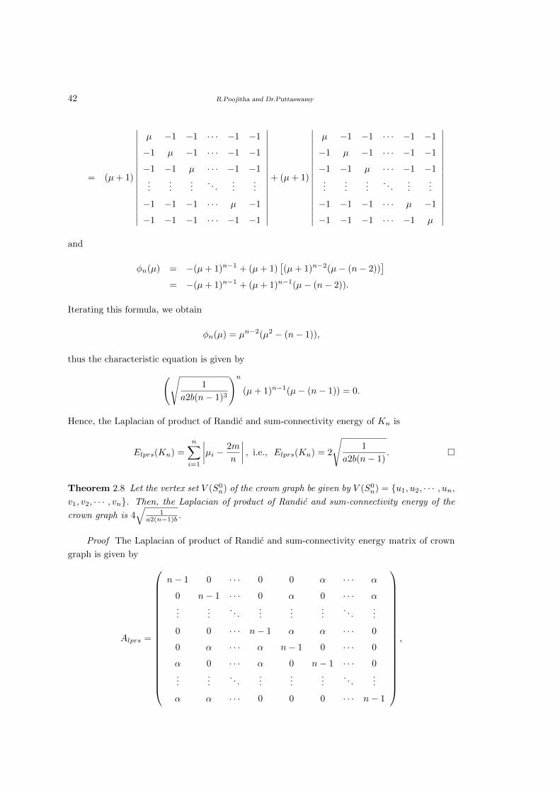
42 R.Poojitha and Dr.Puttaswamy
= (µ+ 1)
∣∣∣∣∣∣∣∣∣∣∣∣∣∣∣∣∣
µ −1 −1 · · · −1 −1
−1 µ −1 · · · −1 −1
−1 −1 µ · · · −1 −1...
......
. . ....
...
−1 −1 −1 · · · µ −1
−1 −1 −1 · · · −1 −1
∣∣∣∣∣∣∣∣∣∣∣∣∣∣∣∣∣+ (µ+ 1)
∣∣∣∣∣∣∣∣∣∣∣∣∣∣∣∣∣
µ −1 −1 · · · −1 −1
−1 µ −1 · · · −1 −1
−1 −1 µ · · · −1 −1...
......
. . ....
...
−1 −1 −1 · · · µ −1
−1 −1 −1 · · · −1 µ
∣∣∣∣∣∣∣∣∣∣∣∣∣∣∣∣∣and
φn(µ) = −(µ+ 1)n−1 + (µ+ 1)[(µ+ 1)n−2(µ− (n− 2))
]= −(µ+ 1)n−1 + (µ+ 1)n−1(µ− (n− 2)).
Iterating this formula, we obtain
φn(µ) = µn−2(µ2 − (n− 1)),
thus the characteristic equation is given by(√1
a2b(n− 1)3
)n(µ+ 1)n−1(µ− (n− 1)) = 0.
Hence, the Laplacian of product of Randic and sum-connectivity energy of Kn is
Elprs(Kn) =
n∑i=1
∣∣∣∣µi − 2m
n
∣∣∣∣ , i.e., Elprs(Kn) = 2
√1
a2b(n− 1). �
Theorem 2.8 Let the vertex set V (S0n) of the crown graph be given by V (S0
n) = {u1, u2, · · · , un,v1, v2, · · · , vn}. Then, the Laplacian of product of Randic and sum-connectivity energy of the
crown graph is 4√
1a2(n−1)b .
Proof The Laplacian of product of Randic and sum-connectivity energy matrix of crown
graph is given by
Alprs =
n− 1 0 · · · 0 0 α · · · α
0 n− 1 · · · 0 α 0 · · · α...
.... . .
......
.... . .
...
0 0 · · · n− 1 α α · · · 0
0 α · · · α n− 1 0 · · · 0
α 0 · · · α 0 n− 1 · · · 0...
.... . .
......
.... . .
...
α α · · · 0 0 0 · · · n− 1
,
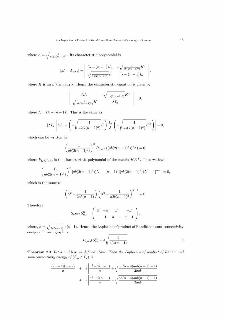
On Laplacian of Product of Randic and Sum-Connectivity Energy of Graphs 43
where α =√
1ab(2(n−1)3) . Its characteristic polynomial is
|λI −Alprs| =
∣∣∣∣∣∣(λ− (n− 1))In −
√1
ab(2(n−1)3)KT√
1ab(2(n−1)3)K (λ− (n− 1)In
∣∣∣∣∣∣ ,where K is an n× n matrix. Hence the characteristic equation is given by∣∣∣∣∣∣
ΛIn −√
1ab(2(n−1)3)K
T√1
ab(2(n−1)3)K ΛIn.
∣∣∣∣∣∣ = 0,
where Λ = (λ− (n− 1)). This is the same as
|ΛIn|
∣∣∣∣∣ΛIn −(−
√1
ab(2(n− 1)3)K
)InΛ
(−
√1
ab(2(n− 1)3)KT
)∣∣∣∣∣ = 0,
which can be written as(1
ab(2(n− 1)3)
)nPKKT ((ab(2(n− 1)3))Λ2) = 0,
where PKKT (Λ) is the characteristic polynomial of the matrix KKT . Thus we have(1)
ab(2(n− 1)3)
)n[ab(2(n− 1)3))Λ2 − (n− 1)2][ab(2(n− 1)3))Λ2 − 1]n−1 = 0,
which is the same as (Λ2 − 1
2ab(n− 1)
)(Λ2 − 1
a2b(n− 1)3
)n−1
= 0.
Therefore
Spec (S0n) =
β −β β −β
1 1 n− 1 n− 1
,
where, β =√
12ab(n−1) +(n−1). Hence, the Laplacian of product of Randic and sum-connectivity
energy of crown graph is
Elprs(S0n) = 4
√1
a2b(n− 1). �
Theorem 2.9 Let a and b be as defined above. Then the Laplacian of product of Randic and
sum-connectivity energy of (Sm ∧ P2) is
(2n− 4)(n− 2)
n+ 2
∣∣∣∣∣n2 − 2(n− 1)
n+
√an3b− 4(anb(n− 1)− 1)
2nab
∣∣∣∣∣+ 2
∣∣∣∣∣n2 − 2(n− 1)
n−√an3b− 4(anb(n− 1)− 1)
2nab
∣∣∣∣∣ .
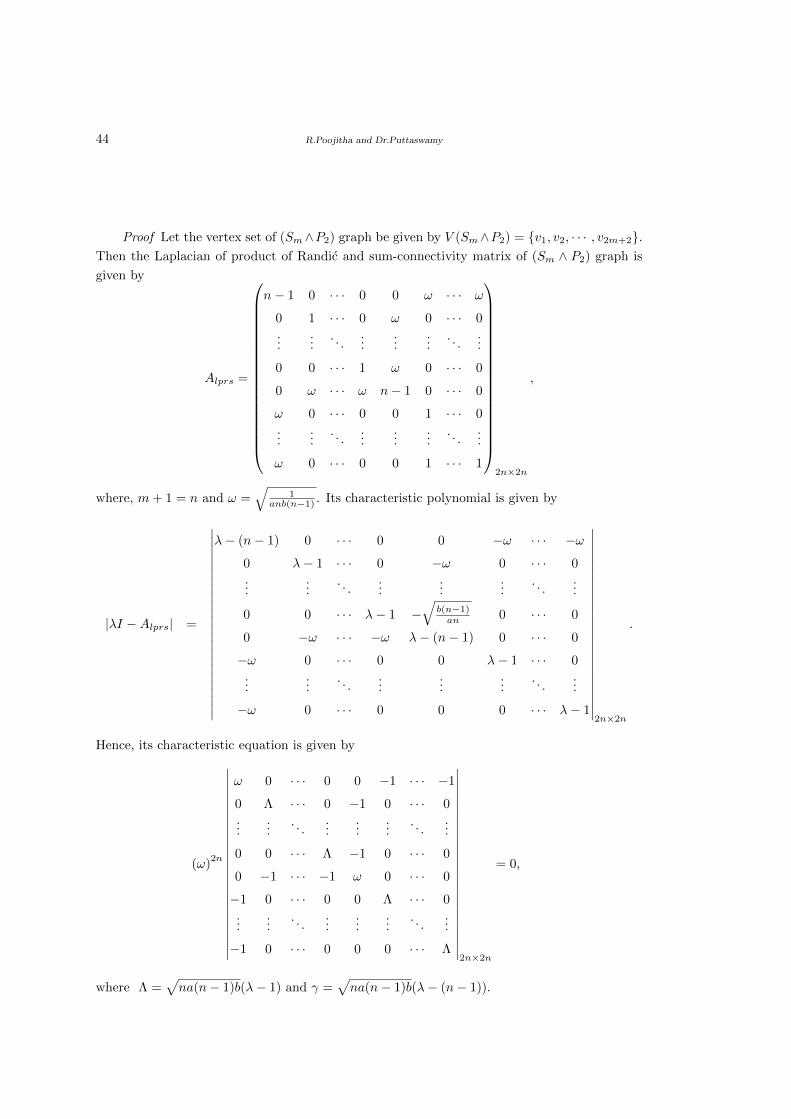
44 R.Poojitha and Dr.Puttaswamy
Proof Let the vertex set of (Sm∧P2) graph be given by V (Sm∧P2) = {v1, v2, · · · , v2m+2}.Then the Laplacian of product of Randic and sum-connectivity matrix of (Sm ∧ P2) graph is
given by
Alprs =
n− 1 0 · · · 0 0 ω · · · ω
0 1 · · · 0 ω 0 · · · 0...
.... . .
......
.... . .
...
0 0 · · · 1 ω 0 · · · 0
0 ω · · · ω n− 1 0 · · · 0
ω 0 · · · 0 0 1 · · · 0...
.... . .
......
.... . .
...
ω 0 · · · 0 0 1 · · · 1
2n×2n
,
where, m+ 1 = n and ω =√
1anb(n−1) . Its characteristic polynomial is given by
|λI −Alprs| =
∣∣∣∣∣∣∣∣∣∣∣∣∣∣∣∣∣∣∣∣∣∣∣∣
λ− (n− 1) 0 · · · 0 0 −ω · · · −ω
0 λ− 1 · · · 0 −ω 0 · · · 0...
.... . .
......
.... . .
...
0 0 · · · λ− 1 −√
b(n−1)an 0 · · · 0
0 −ω · · · −ω λ− (n− 1) 0 · · · 0
−ω 0 · · · 0 0 λ− 1 · · · 0...
.... . .
......
.... . .
...
−ω 0 · · · 0 0 0 · · · λ− 1
∣∣∣∣∣∣∣∣∣∣∣∣∣∣∣∣∣∣∣∣∣∣∣∣2n×2n
.
Hence, its characteristic equation is given by
(ω)2n
∣∣∣∣∣∣∣∣∣∣∣∣∣∣∣∣∣∣∣∣∣∣∣∣
ω 0 · · · 0 0 −1 · · · −1
0 Λ · · · 0 −1 0 · · · 0...
.... . .
......
.... . .
...
0 0 · · · Λ −1 0 · · · 0
0 −1 · · · −1 ω 0 · · · 0
−1 0 · · · 0 0 Λ · · · 0...
.... . .
......
.... . .
...
−1 0 · · · 0 0 0 · · · Λ
∣∣∣∣∣∣∣∣∣∣∣∣∣∣∣∣∣∣∣∣∣∣∣∣2n×2n
= 0,
where Λ =√na(n− 1)b(λ− 1) and γ =
√na(n− 1)b(λ− (n− 1)).
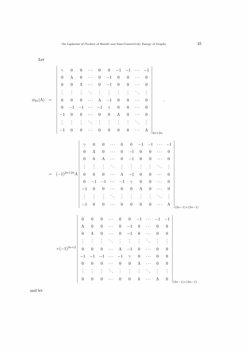
On Laplacian of Product of Randic and Sum-Connectivity Energy of Graphs 45
Let
φ2n(Λ) =
∣∣∣∣∣∣∣∣∣∣∣∣∣∣∣∣∣∣∣∣∣∣∣∣∣∣∣
γ 0 0 · · · 0 0 −1 −1 · · · −1
0 Λ 0 · · · 0 −1 0 0 · · · 0
0 0 Λ · · · 0 −1 0 0 · · · 0...
......
. . ....
......
.... . .
...
0 0 0 · · · Λ −1 0 0 · · · 0
0 −1 −1 · · · −1 γ 0 0 · · · 0
−1 0 0 · · · 0 0 Λ 0 · · · 0...
......
. . ....
......
.... . .
...
−1 0 0 · · · 0 0 0 0 · · · Λ
∣∣∣∣∣∣∣∣∣∣∣∣∣∣∣∣∣∣∣∣∣∣∣∣∣∣∣2n×2n
.
= (−1)2n+2nΛ
∣∣∣∣∣∣∣∣∣∣∣∣∣∣∣∣∣∣∣∣∣∣∣∣∣∣∣
γ 0 0 · · · 0 0 −1 −1 · · · −1
0 Λ 0 · · · 0 −1 0 0 · · · 0
0 0 Λ · · · 0 −1 0 0 · · · 0...
......
. . ....
......
.... . .
...
0 0 0 · · · Λ −1 0 0 · · · 0
0 −1 −1 · · · −1 γ 0 0 · · · 0
−1 0 0 · · · 0 0 Λ 0 · · · 0...
......
. . ....
......
.... . .
...
−1 0 0 · · · 0 0 0 0 · · · Λ
∣∣∣∣∣∣∣∣∣∣∣∣∣∣∣∣∣∣∣∣∣∣∣∣∣∣∣(2n−1)×(2n−1)
+(−1)2n+2
∣∣∣∣∣∣∣∣∣∣∣∣∣∣∣∣∣∣∣∣∣∣∣∣∣∣∣
0 0 0 · · · 0 0 −1 · · · −1 −1
Λ 0 0 · · · 0 −1 0 · · · 0 0
0 Λ 0 · · · 0 −1 0 · · · 0 0...
......
. . ....
......
. . ....
...
0 0 0 · · · Λ −1 0 · · · 0 0
−1 −1 −1 · · · −1 γ 0 · · · 0 0
0 0 0 · · · 0 0 Λ · · · 0 0...
......
. . ....
......
. . ....
...
0 0 0 · · · 0 0 0 · · · Λ 0
∣∣∣∣∣∣∣∣∣∣∣∣∣∣∣∣∣∣∣∣∣∣∣∣∣∣∣(2n−1)×(2n−1)
and let
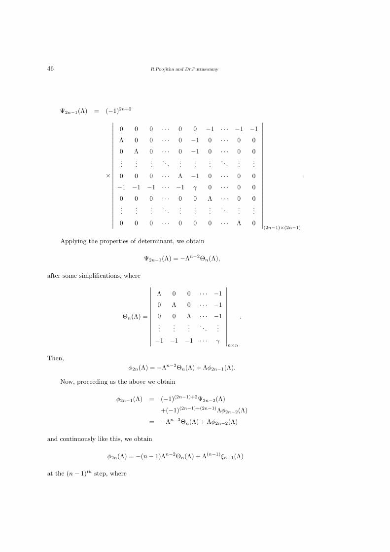
46 R.Poojitha and Dr.Puttaswamy
Ψ2n−1(Λ) = (−1)2n+2
×
∣∣∣∣∣∣∣∣∣∣∣∣∣∣∣∣∣∣∣∣∣∣∣∣∣∣∣
0 0 0 · · · 0 0 −1 · · · −1 −1
Λ 0 0 · · · 0 −1 0 · · · 0 0
0 Λ 0 · · · 0 −1 0 · · · 0 0...
......
. . ....
......
. . ....
...
0 0 0 · · · Λ −1 0 · · · 0 0
−1 −1 −1 · · · −1 γ 0 · · · 0 0
0 0 0 · · · 0 0 Λ · · · 0 0...
......
. . ....
......
. . ....
...
0 0 0 · · · 0 0 0 · · · Λ 0
∣∣∣∣∣∣∣∣∣∣∣∣∣∣∣∣∣∣∣∣∣∣∣∣∣∣∣(2n−1)×(2n−1)
.
Applying the properties of determinant, we obtain
Ψ2n−1(Λ) = −Λn−2Θn(Λ),
after some simplifications, where
Θn(Λ) =
∣∣∣∣∣∣∣∣∣∣∣∣∣∣∣
Λ 0 0 · · · −1
0 Λ 0 · · · −1
0 0 Λ · · · −1...
......
. . ....
−1 −1 −1 · · · γ
∣∣∣∣∣∣∣∣∣∣∣∣∣∣∣n×n
.
Then,
φ2n(Λ) = −Λn−2Θn(Λ) + Λφ2n−1(Λ).
Now, proceeding as the above we obtain
φ2n−1(Λ) = (−1)(2n−1)+2Ψ2n−2(Λ)
+(−1)(2n−1)+(2n−1)Λφ2n−2(Λ)
= −Λn−3Θn(Λ) + Λφ2n−2(Λ)
and continuously like this, we obtain
φ2n(Λ) = −(n− 1)Λn−2Θn(Λ) + Λ(n−1)ξn+1(Λ)
at the (n− 1)th step, where
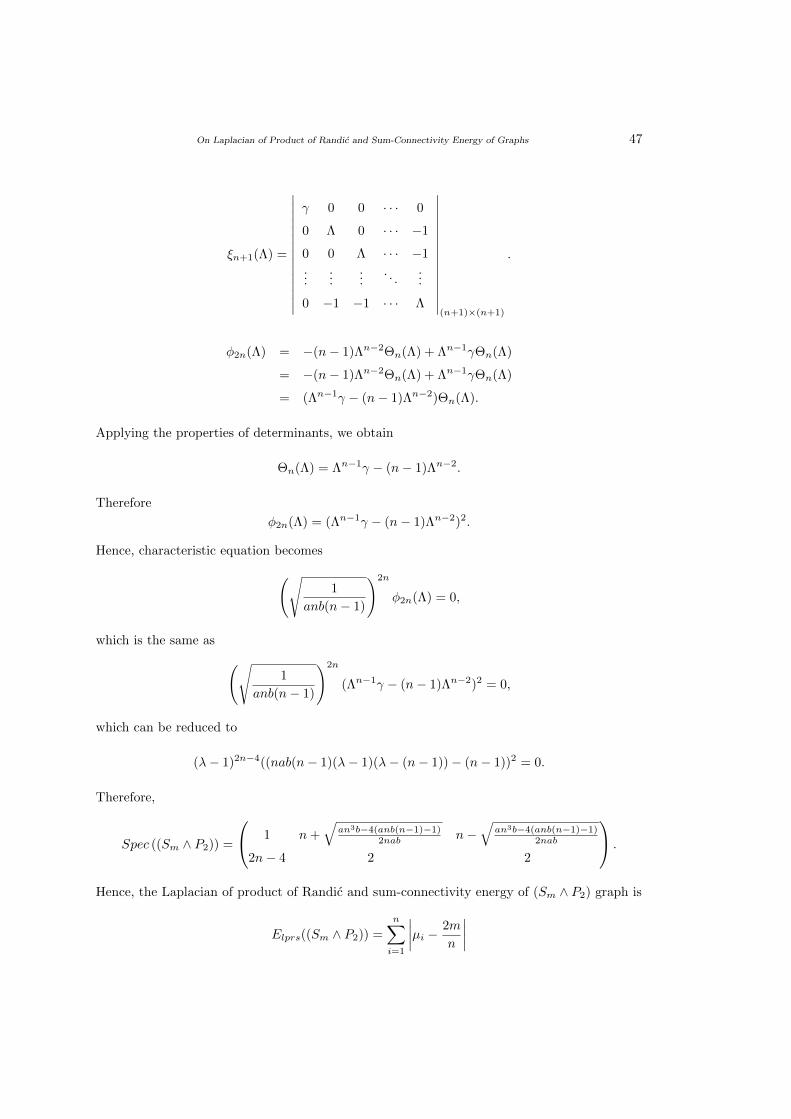
On Laplacian of Product of Randic and Sum-Connectivity Energy of Graphs 47
ξn+1(Λ) =
∣∣∣∣∣∣∣∣∣∣∣∣∣∣∣
γ 0 0 · · · 0
0 Λ 0 · · · −1
0 0 Λ · · · −1...
......
. . ....
0 −1 −1 · · · Λ
∣∣∣∣∣∣∣∣∣∣∣∣∣∣∣(n+1)×(n+1)
.
φ2n(Λ) = −(n− 1)Λn−2Θn(Λ) + Λn−1γΘn(Λ)
= −(n− 1)Λn−2Θn(Λ) + Λn−1γΘn(Λ)
= (Λn−1γ − (n− 1)Λn−2)Θn(Λ).
Applying the properties of determinants, we obtain
Θn(Λ) = Λn−1γ − (n− 1)Λn−2.
Therefore
φ2n(Λ) = (Λn−1γ − (n− 1)Λn−2)2.
Hence, characteristic equation becomes(√1
anb(n− 1)
)2n
φ2n(Λ) = 0,
which is the same as (√1
anb(n− 1)
)2n
(Λn−1γ − (n− 1)Λn−2)2 = 0,
which can be reduced to
(λ− 1)2n−4((nab(n− 1)(λ− 1)(λ− (n− 1))− (n− 1))2 = 0.
Therefore,
Spec ((Sm ∧ P2)) =
1 n+√
an3b−4(anb(n−1)−1)2nab n−
√an3b−4(anb(n−1)−1)
2nab
2n− 4 2 2
.
Hence, the Laplacian of product of Randic and sum-connectivity energy of (Sm ∧ P2) graph is
Elprs((Sm ∧ P2)) =
n∑i=1
∣∣∣∣µi − 2m
n
∣∣∣∣
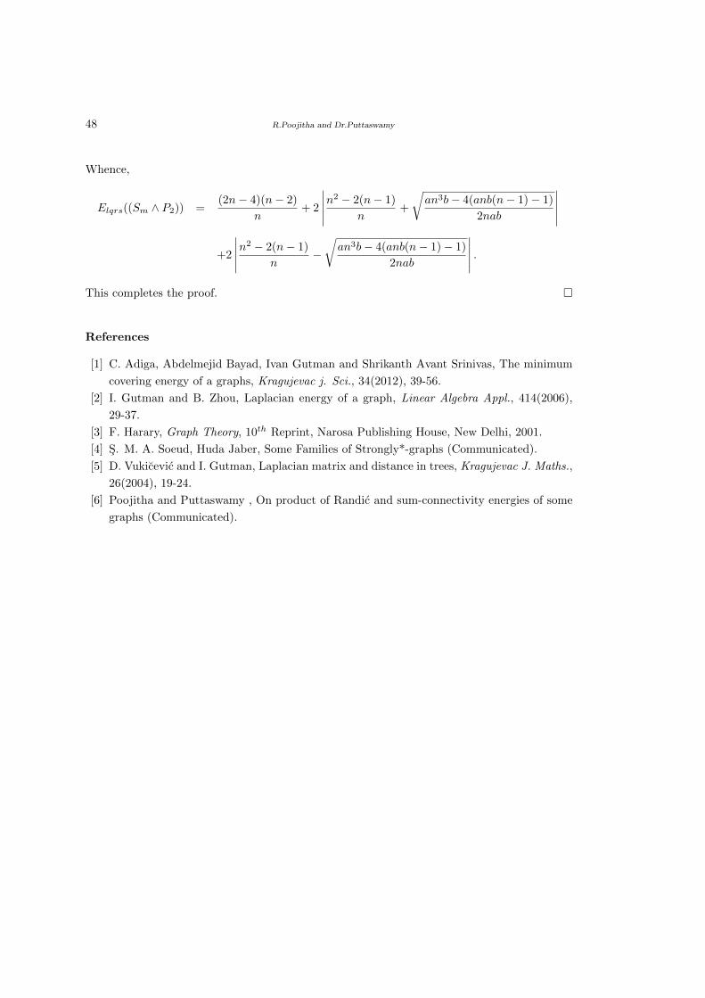
48 R.Poojitha and Dr.Puttaswamy
Whence,
Elqrs((Sm ∧ P2)) =(2n− 4)(n− 2)
n+ 2
∣∣∣∣∣n2 − 2(n− 1)
n+
√an3b− 4(anb(n− 1)− 1)
2nab
∣∣∣∣∣+2
∣∣∣∣∣n2 − 2(n− 1)
n−√an3b− 4(anb(n− 1)− 1)
2nab
∣∣∣∣∣ .This completes the proof. �
References
[1] C. Adiga, Abdelmejid Bayad, Ivan Gutman and Shrikanth Avant Srinivas, The minimum
covering energy of a graphs, Kragujevac j. Sci., 34(2012), 39-56.
[2] I. Gutman and B. Zhou, Laplacian energy of a graph, Linear Algebra Appl., 414(2006),
29-37.
[3] F. Harary, Graph Theory, 10th Reprint, Narosa Publishing House, New Delhi, 2001.
[4] S. M. A. Soeud, Huda Jaber, Some Families of Strongly*-graphs (Communicated).
[5] D. Vukicevic and I. Gutman, Laplacian matrix and distance in trees, Kragujevac J. Maths.,
26(2004), 19-24.
[6] Poojitha and Puttaswamy , On product of Randic and sum-connectivity energies of some
graphs (Communicated).
International J.Math. Combin. Vol.3(2021), 49-61
On Skew-Sum Eccentricity Energy of Digraphs
C. A. Bhavya and Dr.Puttaswamy
(Department of Mathematics, P.E.S. college of Engineering, Mandya-571401, India)
E-mail: [email protected], [email protected]
Abstract: In this paper we introduce the concept of skew-sum eccentricity energy of
directed graphs. We obtain upper and lower bounds for skew-sum eccentricity energy of
digraphs. Then we compute the skew-sum eccentricity energy of some graphs such as star
digraph, complete bipartite digraph, the (Sm∧P2) digraph, (n, 2n−3) strong vertex graceful
digraph and a crown digraph.
Key Words: Energy, eccentricity, skew-sum eccentricity energy, digraph.
AMS(2010): 05C50.
§1. Introduction
In 2018, B. Sharada and Mohammad Issa Ahmed Sowaity [5] introduced the sum eccentricity
energy of a simple graph G as follows. The sum eccentricity adjacency matrix of G is the n×nmatrix (aij), where
aij =
e(vi) + e(vj), if the vertices vi and vj are adjacent,
0, otherwise.
The sum eccentricity energy of G is defined as the sum of absolute values of the eigenvalues
of the sum eccentricity adjacency matrix of G.
In 2010, Adiga, Balakrishnan and Wasin So [1] introduced the skew energy of a digraph
as follows. Let D be a digraph of order n with vertex set V (D) = {v1, v2, · · · , vn} and arc set
Γ(D) ⊂ V (D)×V (D) where (vi, vi) 6∈ Γ(D) for all i and (vi, vj) ∈ Γ(D) implies (vj , vi) 6∈ Γ(D).
The skew-adjacency matrix of D is the n × n matrix S(D) = (sij) where sij = 1 whenever
(vi, vj) ∈ Γ(D), sij = −1 whenever (vj , vi) ∈ Γ(D) and sij = 0 otherwise. Hence S(D) is a
skew symmetric matrix of order n and all its eigenvalues are of the form iλ where i =√−1 and
λ is a real number. The skew energy of G is the sum of the absolute values of eigenvalues of
S(D).
Motivated by these works, we introduce the concept of skew-sum eccentricity energy of a
digraph as follows. Let D be a digraph of order n with vertex set V (D) = {v1, v2, · · · , vn}and arc set Γ(D) ⊂ V (D) × V (D) where (vi, vi) 6∈ Γ(D) for all i and (vi, vj) ∈ Γ(D) implies
(vj , vi) 6∈ Γ(D). Then the skew-sum eccentricity adjacency matrix of D is the n × n matrix
1Received August 11, 2021, Accepted August 31, 2021.
50 C. A. Bhavya and Dr.Puttaswamy
Asse = (aij) where,
aij =
e(vi) + e(vj), if (vi, vj) ∈ Γ(D),
− (e(vi) + e(vj)) , if (vj , vi) ∈ Γ(D),
0, otherwise.
Then the skew-sum eccentricity energy Esse(D) of D is defined as the sum of the absolute
values of eigenvalues of Asse. For example, let D be the directed circle on 4 vertices with the
arc set {(1, 2), (2, 3), (3, 4), (4, 1)}. Then
Asse =
0 4 0 −4
−4 0 4 0
0 −4 0 4
4 0 −4 0
.
with the characteristic equation λ4 + 64λ2 = 0. Its eigenvalues are 8i, 0, 0, −8i and the
skew-sum eccentricity energy of D is 16.
In section 2 of this paper we obtain the upper and lower bounds for skew-sum eccentricity
energy of digraphs. In Section 3 we compute the skew-sum eccentricity energy of some directed
graphs such as complete bipartite digraph, star digraph, the (Sm ∧ P2) digraph, (n, 2n − 3)
strong vertex graceful digraph and a crown digraph.
§2. Upper and Lower Bounds for Skew-Sum Eccentricity Energy
Theorem 2.1 Let D be a simple digraph of order n. Then
Esse(D) ≤√
2n∑j∼k
(e(vj) + e(vk))2.
Proof Let iλ1, iλ2, iλ3, · · · , iλn, be the eigenvalues of Asse, where λ1 ≥ λ2 ≥ λ3 ≥ λ4 ≥· · · ≥ λn. Since
n∑j=1
(iλj)2 = tr(A2
sse) = −n∑j=1
n∑k=1
a2jk = −2
∑j∼k
(e(vj) + e(vk))2,
we haven∑j=1
|λj |2 = 2∑j∼k
(e(vj) + e(vk))2. (1)
Applying the Cauchy-Schwartz inequality n∑j=1
ajbj
2
≤
n∑j=1
a2j
.
n∑j=1
b2j
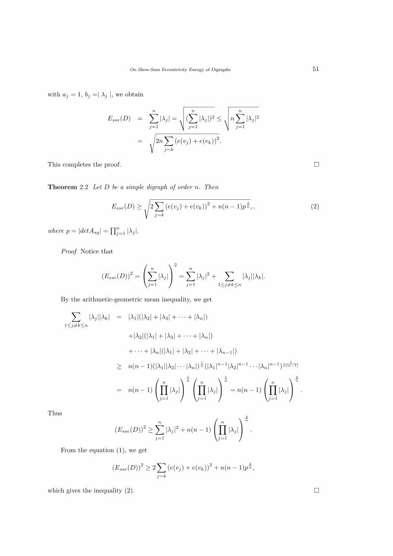
On Skew-Sum Eccentricity Energy of Digraphs 51
with aj = 1, bj =| λj |, we obtain
Esse(D) =
n∑j=1
|λj | =
√√√√(
n∑j=1
|λj |)2 ≤
√√√√n
n∑j=1
|λj |2
=
√2n∑j∼k
(e(vj) + e(vk))2.
This completes the proof. �
Theorem 2.2 Let D be a simple digraph of order n. Then
Esse(D) ≥√
2∑j∼k
(e(vj) + e(vk))2
+ n(n− 1)p2n , . (2)
where p = |detAsg| =∏nj=1 |λj |.
Proof Notice that
(Esse(D))2
=
n∑j=1
|λj |
2
=
n∑j=1
|λj |2 +∑
1≤j 6=k≤n
|λj ||λk|.
By the arithmetic-geometric mean inequality, we get∑1≤j 6=k≤n
|λj ||λk| = |λ1|(|λ2|+ |λ3|+ · · ·+ |λn|)
+|λ2|(|λ1|+ |λ3|+ · · ·+ |λn|)
+ · · ·+ |λn|(|λ1|+ |λ2|+ · · ·+ |λn−1|)
≥ n(n− 1)(|λ1||λ2| · · · |λn|)1n (|λ1|n−1|λ2|n−1 · · · |λn|n−1)
1n(n−1)
= n(n− 1)
n∏j=1
|λj |
1n n∏j=1
|λj |
1n
= n(n− 1)
n∏j=1
|λj |
2n
.
Thus
(Esse(D))2 ≥
n∑j=1
|λj |2 + n(n− 1)
n∏j=1
|λj |
2n
.
From the equation (1), we get
(Esse(D))2 ≥ 2
∑j∼k
(e(vj) + e(vk))2
+ n(n− 1)p2n ,
which gives the inequality (2). �
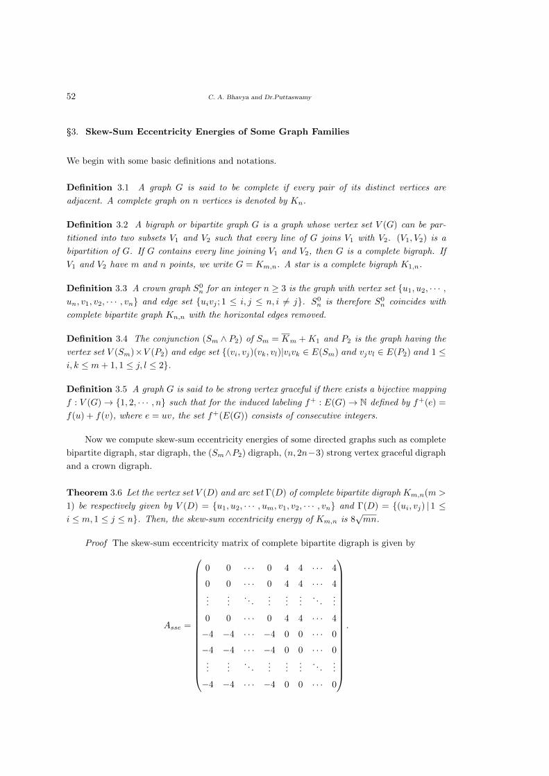
52 C. A. Bhavya and Dr.Puttaswamy
§3. Skew-Sum Eccentricity Energies of Some Graph Families
We begin with some basic definitions and notations.
Definition 3.1 A graph G is said to be complete if every pair of its distinct vertices are
adjacent. A complete graph on n vertices is denoted by Kn.
Definition 3.2 A bigraph or bipartite graph G is a graph whose vertex set V (G) can be par-
titioned into two subsets V1 and V2 such that every line of G joins V1 with V2. (V1, V2) is a
bipartition of G. If G contains every line joining V1 and V2, then G is a complete bigraph. If
V1 and V2 have m and n points, we write G = Km,n. A star is a complete bigraph K1,n.
Definition 3.3 A crown graph S0n for an integer n ≥ 3 is the graph with vertex set {u1, u2, · · · ,
un, v1, v2, · · · , vn} and edge set {uivj ; 1 ≤ i, j ≤ n, i 6= j}. S0n is therefore S0
n coincides with
complete bipartite graph Kn,n with the horizontal edges removed.
Definition 3.4 The conjunction (Sm ∧ P2) of Sm = Km +K1 and P2 is the graph having the
vertex set V (Sm)×V (P2) and edge set {(vi, vj)(vk, vl)|vivk ∈ E(Sm) and vjvl ∈ E(P2) and 1 ≤i, k ≤ m+ 1, 1 ≤ j, l ≤ 2}.
Definition 3.5 A graph G is said to be strong vertex graceful if there exists a bijective mapping
f : V (G)→ {1, 2, · · · , n} such that for the induced labeling f+ : E(G)→ N defined by f+(e) =
f(u) + f(v), where e = uv, the set f+(E(G)) consists of consecutive integers.
Now we compute skew-sum eccentricity energies of some directed graphs such as complete
bipartite digraph, star digraph, the (Sm∧P2) digraph, (n, 2n−3) strong vertex graceful digraph
and a crown digraph.
Theorem 3.6 Let the vertex set V (D) and arc set Γ(D) of complete bipartite digraph Km,n(m >
1) be respectively given by V (D) = {u1, u2, · · · , um, v1, v2, · · · , vn} and Γ(D) = {(ui, vj) | 1 ≤i ≤ m, 1 ≤ j ≤ n}. Then, the skew-sum eccentricity energy of Km,n is 8
√mn.
Proof The skew-sum eccentricity matrix of complete bipartite digraph is given by
Asse =
0 0 · · · 0 4 4 · · · 4
0 0 · · · 0 4 4 · · · 4...
.... . .
......
.... . .
...
0 0 · · · 0 4 4 · · · 4
−4 −4 · · · −4 0 0 · · · 0
−4 −4 · · · −4 0 0 · · · 0...
.... . .
......
.... . .
...
−4 −4 · · · −4 0 0 · · · 0
.
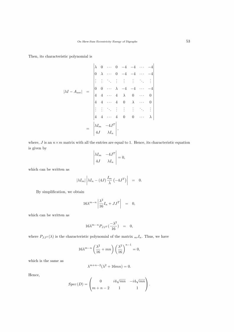
On Skew-Sum Eccentricity Energy of Digraphs 53
Then, its characteristic polynomial is
|λI −Asse| =
∣∣∣∣∣∣∣∣∣∣∣∣∣∣∣∣∣∣∣∣∣∣∣∣
λ 0 · · · 0 −4 −4 · · · −4
0 λ · · · 0 −4 −4 · · · −4...
.... . .
......
.... . .
...
0 0 · · · λ −4 −4 · · · −4
4 4 · · · 4 λ 0 · · · 0
4 4 · · · 4 0 λ · · · 0...
.... . .
......
.... . .
...
4 4 · · · 4 0 0 · · · λ
∣∣∣∣∣∣∣∣∣∣∣∣∣∣∣∣∣∣∣∣∣∣∣∣=
∣∣∣∣∣∣λIm −4JT
4J λIn
∣∣∣∣∣∣ ,where, J is an n×m matrix with all the entries are equal to 1. Hence, its characteristic equation
is given by ∣∣∣∣∣∣λIm −4JT
4J λIn
∣∣∣∣∣∣ = 0,
which can be written as
|λIm|∣∣∣∣λIn − (4J)
Imλ
(−4JT
)∣∣∣∣ = 0.
By simplification, we obtain
16λm−n∣∣∣∣λ2
16In + JJT
∣∣∣∣ = 0,
which can be written as
16λm−nPJJT (−λ2
16) = 0,
where PJJT (λ) is the characteristic polynomial of the matrix mJn. Thus, we have
16λm−n(λ2
16+mn
)(λ2
16
)n−1
= 0,
which is the same as
λm+n−2(λ2 + 16mn) = 0.
Hence,
Spec (D) =
0 i4√mn −i4
√mn
m+ n− 2 1 1
.
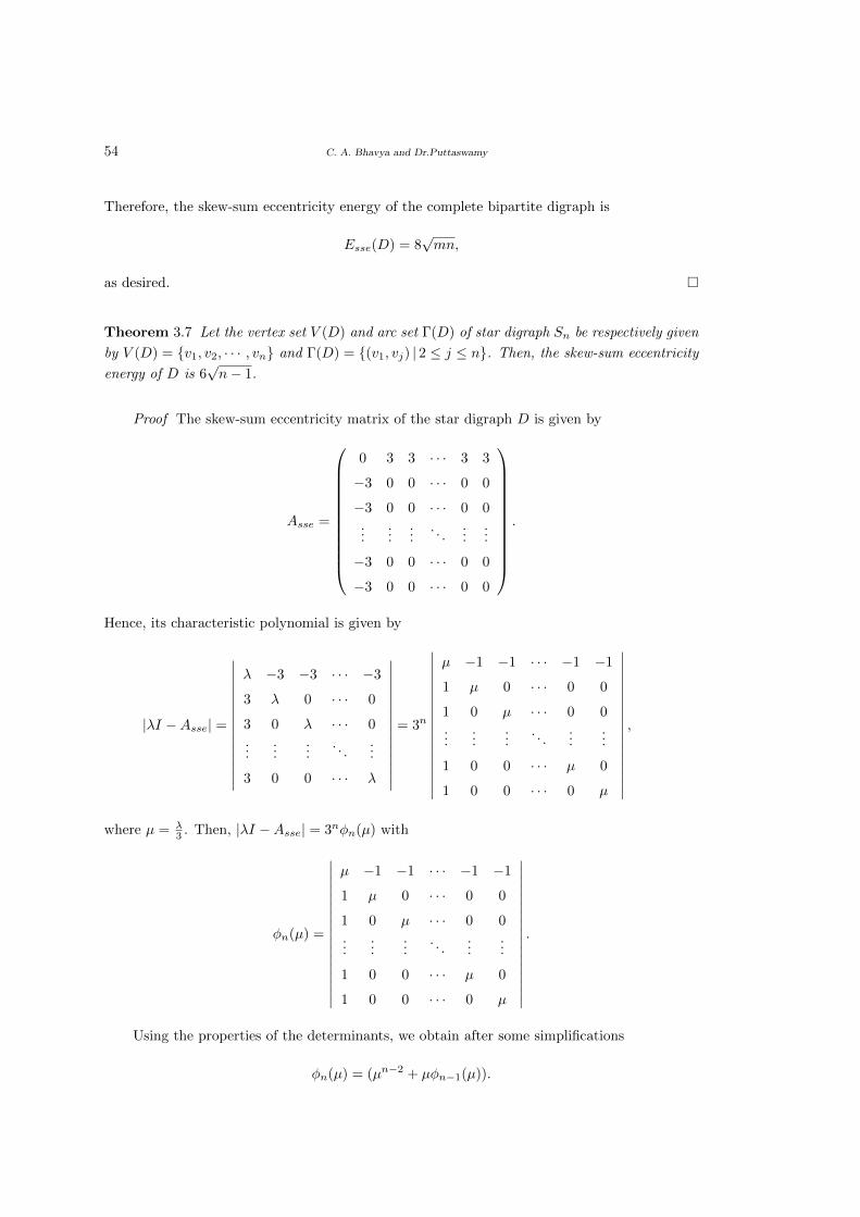
54 C. A. Bhavya and Dr.Puttaswamy
Therefore, the skew-sum eccentricity energy of the complete bipartite digraph is
Esse(D) = 8√mn,
as desired. �
Theorem 3.7 Let the vertex set V (D) and arc set Γ(D) of star digraph Sn be respectively given
by V (D) = {v1, v2, · · · , vn} and Γ(D) = {(v1, vj) | 2 ≤ j ≤ n}. Then, the skew-sum eccentricity
energy of D is 6√n− 1.
Proof The skew-sum eccentricity matrix of the star digraph D is given by
Asse =
0 3 3 · · · 3 3
−3 0 0 · · · 0 0
−3 0 0 · · · 0 0...
......
. . ....
...
−3 0 0 · · · 0 0
−3 0 0 · · · 0 0
.
Hence, its characteristic polynomial is given by
|λI −Asse| =
∣∣∣∣∣∣∣∣∣∣∣∣∣∣∣
λ −3 −3 · · · −3
3 λ 0 · · · 0
3 0 λ · · · 0...
......
. . ....
3 0 0 · · · λ
∣∣∣∣∣∣∣∣∣∣∣∣∣∣∣= 3n
∣∣∣∣∣∣∣∣∣∣∣∣∣∣∣∣∣
µ −1 −1 · · · −1 −1
1 µ 0 · · · 0 0
1 0 µ · · · 0 0...
......
. . ....
...
1 0 0 · · · µ 0
1 0 0 · · · 0 µ
∣∣∣∣∣∣∣∣∣∣∣∣∣∣∣∣∣,
where µ = λ3 . Then, |λI −Asse| = 3nφn(µ) with
φn(µ) =
∣∣∣∣∣∣∣∣∣∣∣∣∣∣∣∣∣
µ −1 −1 · · · −1 −1
1 µ 0 · · · 0 0
1 0 µ · · · 0 0...
......
. . ....
...
1 0 0 · · · µ 0
1 0 0 · · · 0 µ
∣∣∣∣∣∣∣∣∣∣∣∣∣∣∣∣∣.
Using the properties of the determinants, we obtain after some simplifications
φn(µ) = (µn−2 + µφn−1(µ)).
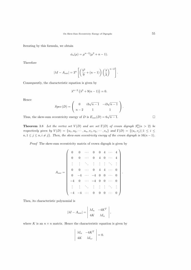
On Skew-Sum Eccentricity Energy of Digraphs 55
Iterating by this formula, we obtain
φn(µ) = µn−2(µ2 + n− 1).
Therefore
|λI −Asse| = 3n
[(λ2
9+ (n− 1)
)(λ
3
)n−2].
Consequently, the characteristic equation is given by
λn−2(λ2 + 9(n− 1)
)= 0.
Hence
Spec (D) =
0 i3√n− 1 −i3
√n− 1
n− 2 1 1
.
Thus, the skew-sum eccentricity energy of D is Esse(D) = 6√n− 1. �
Theorem 3.8 Let the vertex set V (D) and arc set Γ(D) of crown digraph S0n(n > 2) be
respectively given by V (D) = {u1, u2, · · · , un, v1, v2, · · · , vn} and Γ(D) = {(ui, vj) | 1 ≤ i ≤n, 1 ≤ j ≤ n, i 6= j}. Then, the skew-sum eccentricity energy of the crown digraph is 16(n− 1).
Proof The skew-sum eccentricity matrix of crown digraph is given by
Asse =
0 0 · · · 0 0 4 · · · 4
0 0 · · · 0 4 0 · · · 4...
.... . .
......
.... . .
...
0 0 · · · 0 4 4 · · · 0
0 −4 · · · −4 0 0 · · · 0
−4 0 · · · −4 0 0 · · · 0...
.... . .
......
.... . .
...
−4 −4 · · · 0 0 0 · · · 0
.
Then, its characteristic polynomial is
|λI −Asse| =
∣∣∣∣∣∣ λIn −4KT
4K λIn
∣∣∣∣∣∣ ,where K is an n× n matrix. Hence the characteristic equation is given by∣∣∣∣∣∣ λIn −4KT
4K λIn.
∣∣∣∣∣∣ = 0.
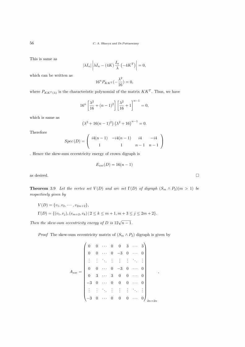
56 C. A. Bhavya and Dr.Puttaswamy
This is same as
|λIn|∣∣∣∣λIn − (4K)
Inλ
(−4KT
)∣∣∣∣ = 0,
which can be written as
16nPKKT (−λ2
16) = 0,
where PKKT (λ) is the characteristic polynomial of the matrix KKT . Thus, we have
16n[λ2
16+ (n− 1)2
] [λ2
16+ 1
]n−1
= 0,
which is same as (λ2 + 16(n− 1)2
) (λ2 + 16
)n−1= 0.
Therefore
Spec (D) =
i4(n− 1) −i4(n− 1) i4 −i4
1 1 n− 1 n− 1
. Hence the skew-sum eccentricity energy of crown digraph is
Esse(D) = 16(n− 1)
as desired. �
Theorem 3.9 Let the vertex set V (D) and arc set Γ(D) of digraph (Sm ∧ P2)(m > 1) be
respectively given by
V (D) = {v1, v2, · · · , v2m+2},
Γ(D) = {(v1, vj), (vm+2, vk) | 2 ≤ k ≤ m+ 1,m+ 3 ≤ j ≤ 2m+ 2}.
Then the skew-sum eccentricity energy of D is 12√n− 1.
Proof The skew-sum eccentricity matrix of (Sm ∧ P2) digraph is given by
Asse =
0 0 · · · 0 0 3 · · · 3
0 0 · · · 0 −3 0 · · · 0...
.... . .
......
.... . .
...
0 0 · · · 0 −3 0 · · · 0
0 3 · · · 3 0 0 · · · 0
−3 0 · · · 0 0 0 · · · 0...
.... . .
......
.... . .
...
−3 0 · · · 0 0 0 · · · 0
2n×2n
,
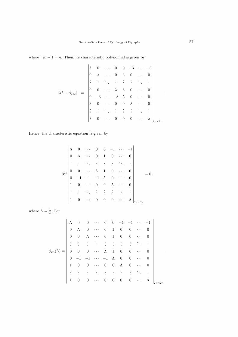
On Skew-Sum Eccentricity Energy of Digraphs 57
where m+ 1 = n. Then, its characteristic polynomial is given by
|λI −Asse| =
∣∣∣∣∣∣∣∣∣∣∣∣∣∣∣∣∣∣∣∣∣∣∣∣
λ 0 · · · 0 0 −3 · · · −3
0 λ · · · 0 3 0 · · · 0...
.... . .
......
.... . .
...
0 0 · · · λ 3 0 · · · 0
0 −3 · · · −3 λ 0 · · · 0
3 0 · · · 0 0 λ · · · 0...
.... . .
......
.... . .
...
3 0 · · · 0 0 0 · · · λ
∣∣∣∣∣∣∣∣∣∣∣∣∣∣∣∣∣∣∣∣∣∣∣∣2n×2n
.
Hence, the characteristic equation is given by
32n
∣∣∣∣∣∣∣∣∣∣∣∣∣∣∣∣∣∣∣∣∣∣∣∣
Λ 0 · · · 0 0 −1 · · · −1
0 Λ · · · 0 1 0 · · · 0...
.... . .
......
.... . .
...
0 0 · · · Λ 1 0 · · · 0
0 −1 · · · −1 Λ 0 · · · 0
1 0 · · · 0 0 Λ · · · 0...
.... . .
......
.... . .
...
1 0 · · · 0 0 0 · · · Λ
∣∣∣∣∣∣∣∣∣∣∣∣∣∣∣∣∣∣∣∣∣∣∣∣2n×2n
= 0,
where Λ = λ3 . Let
φ2n(Λ) =
∣∣∣∣∣∣∣∣∣∣∣∣∣∣∣∣∣∣∣∣∣∣∣∣∣∣∣
Λ 0 0 · · · 0 0 −1 −1 · · · −1
0 Λ 0 · · · 0 1 0 0 · · · 0
0 0 Λ · · · 0 1 0 0 · · · 0...
......
. . ....
......
.... . .
...
0 0 0 · · · Λ 1 0 0 · · · 0
0 −1 −1 · · · −1 Λ 0 0 · · · 0
1 0 0 · · · 0 0 Λ 0 · · · 0...
......
. . ....
......
.... . .
...
1 0 0 · · · 0 0 0 0 · · · Λ
∣∣∣∣∣∣∣∣∣∣∣∣∣∣∣∣∣∣∣∣∣∣∣∣∣∣∣2n×2n
.
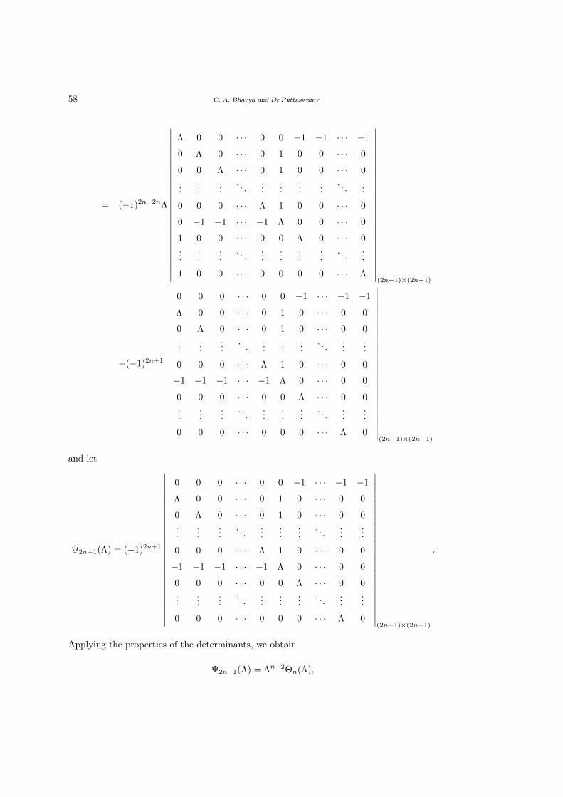
58 C. A. Bhavya and Dr.Puttaswamy
= (−1)2n+2nΛ
∣∣∣∣∣∣∣∣∣∣∣∣∣∣∣∣∣∣∣∣∣∣∣∣∣∣∣
Λ 0 0 · · · 0 0 −1 −1 · · · −1
0 Λ 0 · · · 0 1 0 0 · · · 0
0 0 Λ · · · 0 1 0 0 · · · 0...
......
. . ....
......
.... . .
...
0 0 0 · · · Λ 1 0 0 · · · 0
0 −1 −1 · · · −1 Λ 0 0 · · · 0
1 0 0 · · · 0 0 Λ 0 · · · 0...
......
. . ....
......
.... . .
...
1 0 0 · · · 0 0 0 0 · · · Λ
∣∣∣∣∣∣∣∣∣∣∣∣∣∣∣∣∣∣∣∣∣∣∣∣∣∣∣(2n−1)×(2n−1)
+(−1)2n+1
∣∣∣∣∣∣∣∣∣∣∣∣∣∣∣∣∣∣∣∣∣∣∣∣∣∣∣
0 0 0 · · · 0 0 −1 · · · −1 −1
Λ 0 0 · · · 0 1 0 · · · 0 0
0 Λ 0 · · · 0 1 0 · · · 0 0...
......
. . ....
......
. . ....
...
0 0 0 · · · Λ 1 0 · · · 0 0
−1 −1 −1 · · · −1 Λ 0 · · · 0 0
0 0 0 · · · 0 0 Λ · · · 0 0...
......
. . ....
......
. . ....
...
0 0 0 · · · 0 0 0 · · · Λ 0
∣∣∣∣∣∣∣∣∣∣∣∣∣∣∣∣∣∣∣∣∣∣∣∣∣∣∣(2n−1)×(2n−1)
and let
Ψ2n−1(Λ) = (−1)2n+1
∣∣∣∣∣∣∣∣∣∣∣∣∣∣∣∣∣∣∣∣∣∣∣∣∣∣∣
0 0 0 · · · 0 0 −1 · · · −1 −1
Λ 0 0 · · · 0 1 0 · · · 0 0
0 Λ 0 · · · 0 1 0 · · · 0 0...
......
. . ....
......
. . ....
...
0 0 0 · · · Λ 1 0 · · · 0 0
−1 −1 −1 · · · −1 Λ 0 · · · 0 0
0 0 0 · · · 0 0 Λ · · · 0 0...
......
. . ....
......
. . ....
...
0 0 0 · · · 0 0 0 · · · Λ 0
∣∣∣∣∣∣∣∣∣∣∣∣∣∣∣∣∣∣∣∣∣∣∣∣∣∣∣(2n−1)×(2n−1)
.
Applying the properties of the determinants, we obtain
Ψ2n−1(Λ) = Λn−2Θn(Λ),
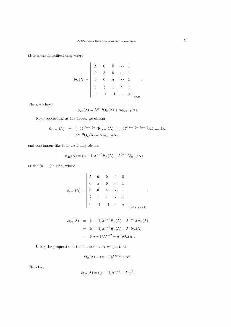
On Skew-Sum Eccentricity Energy of Digraphs 59
after some simplifications, where
Θn(Λ) =
∣∣∣∣∣∣∣∣∣∣∣∣∣∣∣
Λ 0 0 · · · 1
0 Λ 0 · · · 1
0 0 Λ · · · 1...
......
. . ....
−1 −1 −1 · · · Λ
∣∣∣∣∣∣∣∣∣∣∣∣∣∣∣n×n
.
Then, we have
φ2n(Λ) = Λn−2Θn(Λ) + Λφ2n−1(Λ).
Now, proceeding as the above, we obtain
φ2n−1(Λ) = (−1)(2n−1)+1Ψ2n−2(Λ) + (−1)(2n−1)+(2n−1)Λφ2n−2(Λ)
= Λn−3Θn(Λ) + Λφ2n−2(Λ).
and continuous like this, we finally obtain
φ2n(Λ) = (n− 1)Λn−2Θn(Λ) + Λ(n−1)ξn+1(Λ)
at the (n− 1)th step, where
ξn+1(Λ) =
∣∣∣∣∣∣∣∣∣∣∣∣∣∣∣
Λ 0 0 · · · 0
0 Λ 0 · · · 1
0 0 Λ · · · 1...
......
. . ....
0 −1 −1 · · · Λ
∣∣∣∣∣∣∣∣∣∣∣∣∣∣∣(n+1)×(n+1)
.
φ2n(Λ) = (n− 1)Λn−2Θn(Λ) + Λn−1ΛΘn(Λ)
= (n− 1)Λn−2Θn(Λ) + ΛnΘn(Λ)
= ((n− 1)Λn−2 + Λn)Θn(Λ).
Using the properties of the determinants, we get that
Θn(Λ) = (n− 1)Λn−2 + Λn.
Therefore
φ2n(Λ) = ((n− 1)Λn−2 + Λn)2.
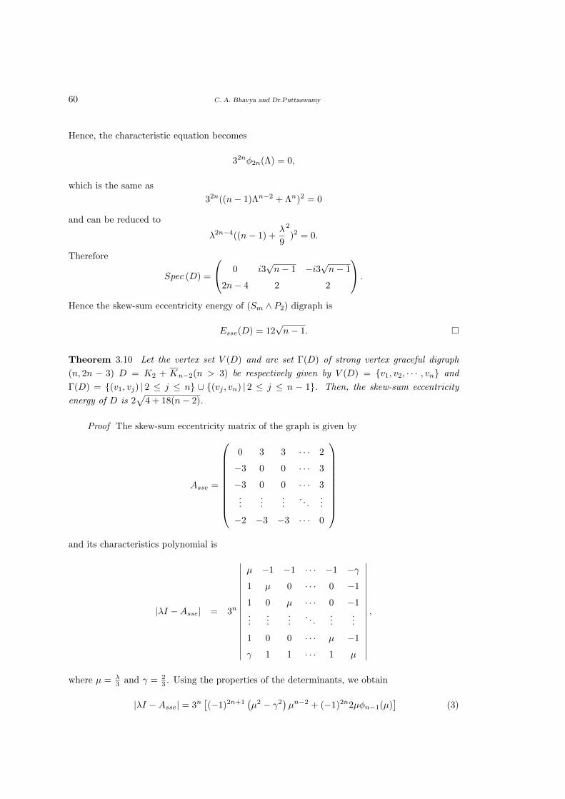
60 C. A. Bhavya and Dr.Puttaswamy
Hence, the characteristic equation becomes
32nφ2n(Λ) = 0,
which is the same as
32n((n− 1)Λn−2 + Λn)2 = 0
and can be reduced to
λ2n−4((n− 1) +λ
9
2
)2 = 0.
Therefore
Spec (D) =
0 i3√n− 1 −i3
√n− 1
2n− 4 2 2
.
Hence the skew-sum eccentricity energy of (Sm ∧ P2) digraph is
Esse(D) = 12√n− 1. �
Theorem 3.10 Let the vertex set V (D) and arc set Γ(D) of strong vertex graceful digraph
(n, 2n − 3) D = K2 + Kn−2(n > 3) be respectively given by V (D) = {v1, v2, · · · , vn} and
Γ(D) = {(v1, vj) | 2 ≤ j ≤ n} ∪ {(vj , vn) | 2 ≤ j ≤ n − 1}. Then, the skew-sum eccentricity
energy of D is 2√
4 + 18(n− 2).
Proof The skew-sum eccentricity matrix of the graph is given by
Asse =
0 3 3 · · · 2
−3 0 0 · · · 3
−3 0 0 · · · 3...
......
. . ....
−2 −3 −3 · · · 0
and its characteristics polynomial is
|λI −Asse| = 3n
∣∣∣∣∣∣∣∣∣∣∣∣∣∣∣∣∣
µ −1 −1 · · · −1 −γ
1 µ 0 · · · 0 −1
1 0 µ · · · 0 −1...
......
. . ....
...
1 0 0 · · · µ −1
γ 1 1 · · · 1 µ
∣∣∣∣∣∣∣∣∣∣∣∣∣∣∣∣∣,
where µ = λ3 and γ = 2
3 . Using the properties of the determinants, we obtain
|λI −Asse| = 3n[(−1)2n+1
(µ2 − γ2
)µn−2 + (−1)2n2µφn−1(µ)
](3)
On Skew-Sum Eccentricity Energy of Digraphs 61
after some simplifications, where
φn−1(µ) =
∣∣∣∣∣∣∣∣∣∣∣∣∣∣∣
µ −1 −1 · · · −1
1 µ 0 · · · 0
1 0 µ · · · 0...
......
. . ....
1 0 0 · · · µ
∣∣∣∣∣∣∣∣∣∣∣∣∣∣∣(n−1)×(n−1)
.
Now, as in the proof of the Theorem 3.7, we obtain
φn−1(µ) = µn−3 + µφn−2(µ).
Iterating with this formula, we obtain
φn−1(µ) = µn−3(µ2 + n− 2). (4)
Substituting (4) in (3) and using µ = λ3 , we obtain
|λI −Asse| = 3n[−(µ2 − γ2
)(µ)n−2 +2(µ)n−2(µ2 + n− 2)
]= 9λn−2
(µ2 + γ2 + 2(n− 2)
).
Thus, the characteristic equation is given by
λn−2
(λ2
9+
4 + 18(n− 2)
9
)= 0.
Hence
Spec (D) =
0 i√
4 + 18(n− 2) −i√
4 + 18(n− 2)
n− 2 1 1
.
So, the skew-sum eccentricity energy of D is Esse(D) = 2√
4 + 18(n− 2) as desired. �
References
[1] C. Adiga, R. Balakrishnan and Wasin So, The skew energy of a digraph, Lin. Algebra
Appl., 432(2010), 1825-1835.
[2] C. Adiga, Abdelmejid Bayad, Ivan Gutman and Shrikanth Avant Srinivas, The minimum
covering energy of a digraph, Kragujevac j. Sci., 34(2012), 39-56.
[3] F. Harary, Graph Theory, 10th Reprint, Narosa Publishing House, New Delhi, 2001.
[4] S. M. A. Soeud, Huda Jaber, Some Families of Strongly*-graphs (Communicated).
[5] B. Sharada, Mohammad issa ahmed sowaity, On the sum-eccentricity energy of a graph
Int. J. Appl. Graph Theory, 22(2018), 1-8.
[6] D. D. Somashekara and C. R. Veena, On strong vertex graceful graphs, International Math.
Forum, 5(2010), 2751-2757.
International J.Math. Combin. Vol.3(2021), 62-76
Computation of (a,b)-KA Indices of Some Special Graphs
V. R. Kulli
(Department of Mathematics, Gulbarga University, Gulbarga - 585 106, India)
D. Vyshnavi and B. Chaluvaraju
(Department of Mathematics, Bangalore University, Jnana Bharathi Campus, Bangalore -560 056, India)
E-mail: [email protected], [email protected], [email protected]
Abstract: The significance of the (a, b) -KA indices lies on the fact that their special cases,
for pertinently chosen values of the parameters a and b, coincide with the vast majority of
previously considered vertex based topological indices. In this paper, we computed the (a, b)
- KA indices of some special class of graphs such as regular graph (hyper cube graph and
generalized petersen graph), cartesian product graph (grid graph, torus graph and cylinder
graph), lollipop graph and Harary graph.
Key Words: Molecular descriptors, (a, b)-KA indices, (a, b)-KA coindices.
AMS(2010): 05C05, 05C07, 05C35.
§1. Introduction
All the graphs considered here are finite, undirected, connected with no loops and multiple
edges. As usual p = |V | and q = |E| denote the number of vertices and edges of a graph
G = (V,E), respectively. The edge connecting the vertices u and v will be denoted by uv. Let
dG(e) denote the degree of an edge e in G, which is defined by dG(e) = dG(u) + dG(v)− 2 with
e = uv. For graph theoretic terminology and notation not given here we refer the reader to
Kulli [15].
Chemical graph theory is a branch of the mathematical chemistry which has an impor-
tant effect on the development of the chemical sciences. A single number that can be used
to characterize some property of the graph of a molecular structure is called a topological in-
dex for that graph. There are numerous molecular descriptors, which are also referred to as
topological indices, that have found some applications in theoretical chemistry, especially in
QSPR/QSAR/QSTR research. For the historical milestones, some applications and mathe-
matical properties of graph theory, we refer to [4, 6, 8, 10, 20, 32].
The first (a, b)-KA index KA1(a,b)(G), the second (a, b)-KA index KA2
(a,b)(G) and the third
(a, b)-KA index KA3(a,b)(G) of a graph G are defined as
KA1(a,b)(G) =
∑uv∈E(G)
[dG(u)a + dG(v)a]b,
1Received July 13, 2021, Accepted September 2, 2021.
Computation of (a,b)-KA Indices of Some Special Graphs 63
KA2(a,b)(G) =
∑uv∈E(G)
[dG(u)a.dG(v)a]b
and
KA3(a,b)(G) =
∑uv∈E(G)
| dG(u)a − dG(v)a |b,
where a and b are real numbers.
These (a, b)-KA indices were introduced by Kulli [21] and elaborated in [24].
§2. The Particular Values of a and b in (a, b)-KA Indices
The majority of hitherto studied vertex degree based topological indices are special cases of
(a, b)-KA indices, for particular values of real numbers a and b as follows:
(1) KA1(1,1)(G) = M1(G), the first Zagreb index, [12].
(2) KA2(1,1)(G) = M2(G), the second Zagreb index, [12].
(3) KA1(−1,1)(G) = RM1(G), the redefined first Zagreb index, [29].
(4) KA1(−1,−1)(G) = RM2(G), the redefined second Zagreb index, [29].
(5) KA1(2,1)(G) = F1(G), the first Forgotten index, [5].
(6) KA2(2,1)(G) = F2(G), the second Forgotten index, [16].
(7) KA1(2,2)(G) = HF1(G), the first hyper Forgotten index, [9].
(8) KA1(1,2)(G) = HM1(G), the first hyper Zagreb index, [31].
(9) KA2(1,2)(G) = HM2(G), the second hyper Zagreb index, [34].
(10) KA1(1,− 1
2 )(G) = χ(G), the sum connectivity index, [35].
(11) KA2(1,− 1
2 )(G) = R(G), the Randic index, [28].
(12) KA2(1, 12 )
(G) = RR(G), the reciprocal Randic index, [15].
(13) 12KA
1(1,1)(G) = SK(G), the SK-index, [30].
(14) KA1(2, 12 )
(G) = SO(G), the Sombor index, [7].
(15) KA3(1,1)(G) = Alb(G), the Albertson (Mi(G) Minus) index, [1].
(16) KA3(−1,1)(G) = Min(G), the misbalance indeg index, [33].
(17) KA3( 12 ,1)
(G) = Mro(G), the misbalance rodeg index, [33].
(18) KA3(− 1
2 ,1)(G) = Mir(G), the misbalance irdeg index, [33].
(19) KA3(1,2)(G) = σ(G), the Sigma index, [11].
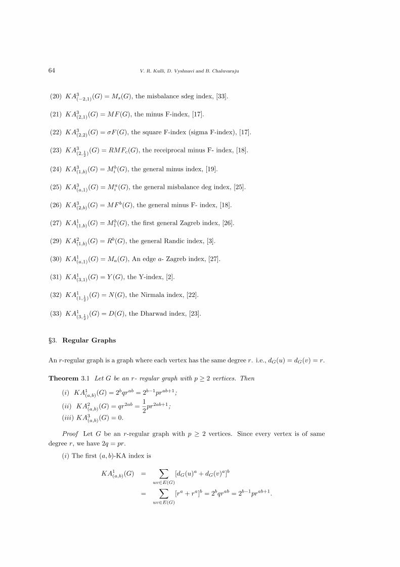
64 V. R. Kulli, D. Vyshnavi and B. Chaluvaraju
(20) KA3(−2,1)(G) = Ms(G), the misbalance sdeg index, [33].
(21) KA3(2,1)(G) = MF (G), the minus F-index, [17].
(22) KA3(2,2)(G) = σF (G), the square F-index (sigma F-index), [17].
(23) KA3(2, 12 )
(G) = RMFc(G), the receiprocal minus F- index, [18].
(24) KA3(1,b)(G) = M b
i (G), the general minus index, [19].
(25) KA3(a,1)(G) = Ma
i (G), the general misbalance deg index, [25].
(26) KA3(2,b)(G) = MF b(G), the general minus F- index, [18].
(27) KA1(1,b)(G) = M b
1(G), the first general Zagreb index, [26].
(29) KA2(1,b)(G) = Rb(G), the general Randic index, [3].
(30) KA1(a,1)(G) = Ma(G), An edge a- Zagreb index, [27].
(31) KA1(3,1)(G) = Y (G), the Y-index, [2].
(32) KA1(1, 12 )
(G) = N(G), the Nirmala index, [22].
(33) KA1(3, 12 )
(G) = D(G), the Dharwad index, [23].
§3. Regular Graphs
An r-regular graph is a graph where each vertex has the same degree r. i.e., dG(u) = dG(v) = r.
Theorem 3.1 Let G be an r- regular graph with p ≥ 2 vertices. Then
(i) KA1(a,b)(G) = 2bqrab = 2b−1prab+1;
(ii) KA2(a,b)(G) = qr2ab =
1
2pr2ab+1;
(iii) KA3(a,b)(G) = 0.
Proof Let G be an r-regular graph with p ≥ 2 vertices. Since every vertex is of same
degree r, we have 2q = pr.
(i) The first (a, b)-KA index is
KA1(a,b)(G) =
∑uv∈E(G)
[dG(u)a + dG(v)a]b
=∑
uv∈E(G)
[ra + ra]b = 2bqrab = 2b−1prab+1.
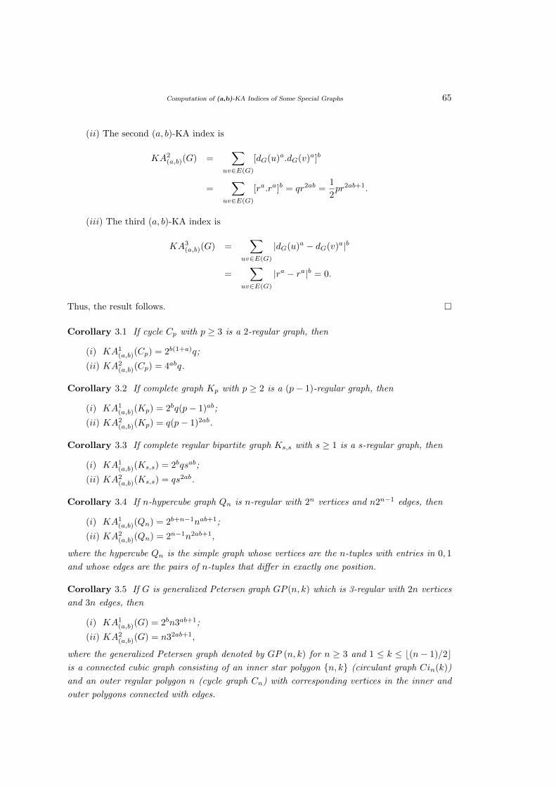
Computation of (a,b)-KA Indices of Some Special Graphs 65
(ii) The second (a, b)-KA index is
KA2(a,b)(G) =
∑uv∈E(G)
[dG(u)a.dG(v)a]b
=∑
uv∈E(G)
[ra.ra]b = qr2ab =1
2pr2ab+1.
(iii) The third (a, b)-KA index is
KA3(a,b)(G) =
∑uv∈E(G)
|dG(u)a − dG(v)a|b
=∑
uv∈E(G)
|ra − ra|b = 0.
Thus, the result follows. �
Corollary 3.1 If cycle Cp with p ≥ 3 is a 2-regular graph, then
(i) KA1(a,b)(Cp) = 2b(1+a)q;
(ii) KA2(a,b)(Cp) = 4abq.
Corollary 3.2 If complete graph Kp with p ≥ 2 is a (p− 1)-regular graph, then
(i) KA1(a,b)(Kp) = 2bq(p− 1)ab;
(ii) KA2(a,b)(Kp) = q(p− 1)2ab.
Corollary 3.3 If complete regular bipartite graph Ks,s with s ≥ 1 is a s-regular graph, then
(i) KA1(a,b)(Ks,s) = 2bqsab;
(ii) KA2(a,b)(Ks,s) = qs2ab.
Corollary 3.4 If n-hypercube graph Qn is n-regular with 2n vertices and n2n−1 edges, then
(i) KA1(a,b)(Qn) = 2b+n−1nab+1;
(ii) KA2(a,b)(Qn) = 2n−1n2ab+1,
where the hypercube Qn is the simple graph whose vertices are the n-tuples with entries in 0, 1
and whose edges are the pairs of n-tuples that differ in exactly one position.
Corollary 3.5 If G is generalized Petersen graph GP (n, k) which is 3-regular with 2n vertices
and 3n edges, then
(i) KA1(a,b)(G) = 2bn3ab+1;
(ii) KA2(a,b)(G) = n32ab+1,
where the generalized Petersen graph denoted by GP (n, k) for n ≥ 3 and 1 ≤ k ≤ b(n− 1)/2cis a connected cubic graph consisting of an inner star polygon {n, k} (circulant graph Cin(k))
and an outer regular polygon n (cycle graph Cn) with corresponding vertices in the inner and
outer polygons connected with edges.
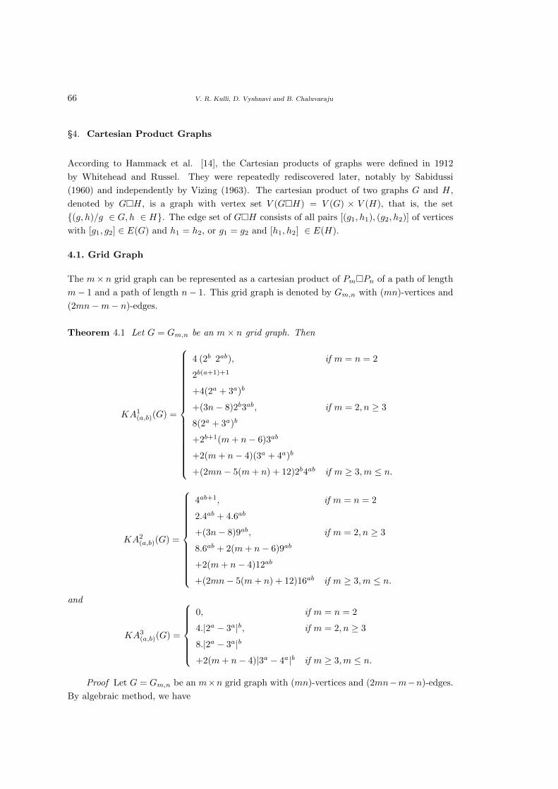
66 V. R. Kulli, D. Vyshnavi and B. Chaluvaraju
§4. Cartesian Product Graphs
According to Hammack et al. [14], the Cartesian products of graphs were defined in 1912
by Whitehead and Russel. They were repeatedly rediscovered later, notably by Sabidussi
(1960) and independently by Vizing (1963). The cartesian product of two graphs G and H,
denoted by G�H, is a graph with vertex set V (G�H) = V (G) × V (H), that is, the set
{(g, h)/g ∈ G, h ∈ H}. The edge set of G�H consists of all pairs [(g1, h1), (g2, h2)] of vertices
with [g1, g2] ∈ E(G) and h1 = h2, or g1 = g2 and [h1, h2] ∈ E(H).
4.1. Grid Graph
The m× n grid graph can be represented as a cartesian product of Pm�Pn of a path of length
m− 1 and a path of length n− 1. This grid graph is denoted by Gm,n with (mn)-vertices and
(2mn−m− n)-edges.
Theorem 4.1 Let G = Gm,n be an m× n grid graph. Then
KA1(a,b)(G) =
4 (2b 2ab), if m = n = 2
2b(a+1)+1
+4(2a + 3a)b
+(3n− 8)2b3ab, if m = 2, n ≥ 3
8(2a + 3a)b
+2b+1(m+ n− 6)3ab
+2(m+ n− 4)(3a + 4a)b
+(2mn− 5(m+ n) + 12)2b4ab if m ≥ 3,m ≤ n.
KA2(a,b)(G) =
4ab+1, if m = n = 2
2.4ab + 4.6ab
+(3n− 8)9ab, if m = 2, n ≥ 3
8.6ab + 2(m+ n− 6)9ab
+2(m+ n− 4)12ab
+(2mn− 5(m+ n) + 12)16ab if m ≥ 3,m ≤ n.
and
KA3(a,b)(G) =
0, if m = n = 2
4.|2a − 3a|b, if m = 2, n ≥ 3
8.|2a − 3a|b
+2(m+ n− 4)|3a − 4a|b if m ≥ 3,m ≤ n.
Proof Let G = Gm,n be an m×n grid graph with (mn)-vertices and (2mn−m−n)-edges.
By algebraic method, we have
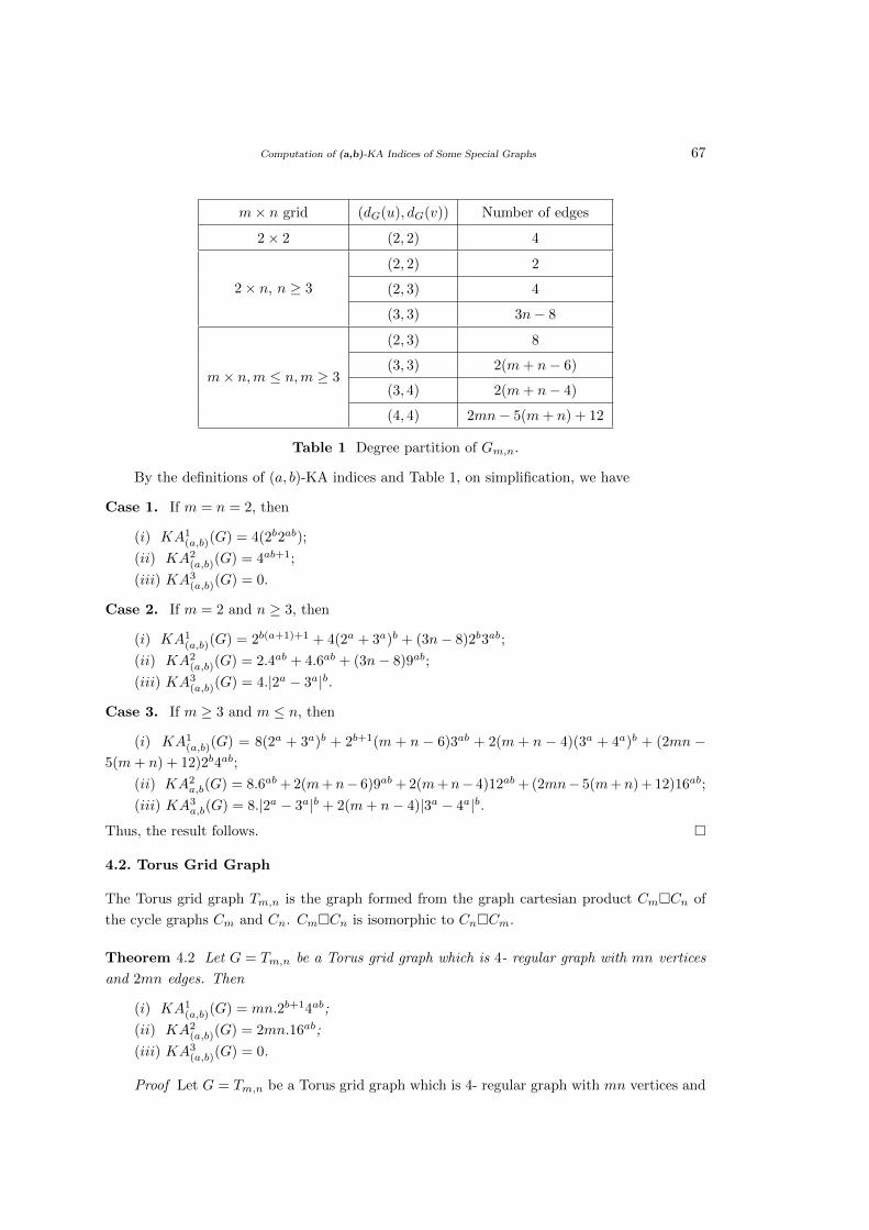
Computation of (a,b)-KA Indices of Some Special Graphs 67
m× n grid (dG(u), dG(v)) Number of edges
2× 2 (2, 2) 4
2× n, n ≥ 3
(2, 2) 2
(2, 3) 4
(3, 3) 3n− 8
m× n,m ≤ n,m ≥ 3
(2, 3) 8
(3, 3) 2(m+ n− 6)
(3, 4) 2(m+ n− 4)
(4, 4) 2mn− 5(m+ n) + 12
Table 1 Degree partition of Gm,n.
By the definitions of (a, b)-KA indices and Table 1, on simplification, we have
Case 1. If m = n = 2, then
(i) KA1(a,b)(G) = 4(2b2ab);
(ii) KA2(a,b)(G) = 4ab+1;
(iii) KA3(a,b)(G) = 0.
Case 2. If m = 2 and n ≥ 3, then
(i) KA1(a,b)(G) = 2b(a+1)+1 + 4(2a + 3a)b + (3n− 8)2b3ab;
(ii) KA2(a,b)(G) = 2.4ab + 4.6ab + (3n− 8)9ab;
(iii) KA3(a,b)(G) = 4.|2a − 3a|b.
Case 3. If m ≥ 3 and m ≤ n, then
(i) KA1(a,b)(G) = 8(2a + 3a)b + 2b+1(m + n − 6)3ab + 2(m + n − 4)(3a + 4a)b + (2mn −
5(m+ n) + 12)2b4ab;
(ii) KA2a,b(G) = 8.6ab + 2(m+n− 6)9ab + 2(m+n− 4)12ab + (2mn− 5(m+n) + 12)16ab;
(iii) KA3a,b(G) = 8.|2a − 3a|b + 2(m+ n− 4)|3a − 4a|b.
Thus, the result follows. �
4.2. Torus Grid Graph
The Torus grid graph Tm,n is the graph formed from the graph cartesian product Cm�Cn of
the cycle graphs Cm and Cn. Cm�Cn is isomorphic to Cn�Cm.
Theorem 4.2 Let G = Tm,n be a Torus grid graph which is 4- regular graph with mn vertices
and 2mn edges. Then
(i) KA1(a,b)(G) = mn.2b+14ab;
(ii) KA2(a,b)(G) = 2mn.16ab;
(iii) KA3(a,b)(G) = 0.
Proof Let G = Tm,n be a Torus grid graph which is 4- regular graph with mn vertices and
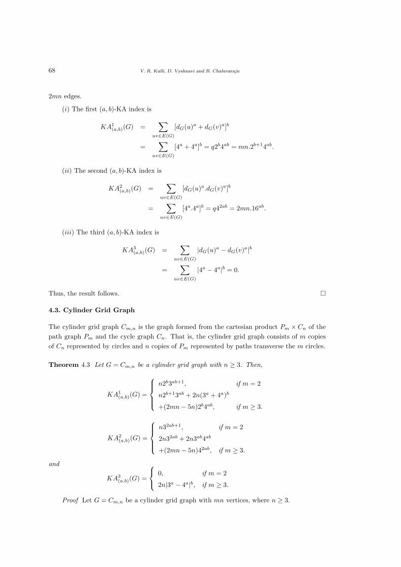
68 V. R. Kulli, D. Vyshnavi and B. Chaluvaraju
2mn edges.
(i) The first (a, b)-KA index is
KA1(a,b)(G) =
∑uv∈E(G)
[dG(u)a + dG(v)a]b
=∑
uv∈E(G)
[4a + 4a]b = q2b4ab = mn.2b+14ab.
(ii) The second (a, b)-KA index is
KA2(a,b)(G) =
∑uv∈E(G)
[dG(u)a.dG(v)a]b
=∑
uv∈E(G)
[4a.4a]b = q42ab = 2mn.16ab.
(iii) The third (a, b)-KA index is
KA3(a,b)(G) =
∑uv∈E(G)
|dG(u)a − dG(v)a|b
=∑
uv∈E(G)
|4a − 4a|b = 0.
Thus, the result follows. �
4.3. Cylinder Grid Graph
The cylinder grid graph Cm,n is the graph formed from the cartesian product Pm × Cn of the
path graph Pm and the cycle graph Cn. That is, the cylinder grid graph consists of m copies
of Cn represented by circles and n copies of Pm represented by paths transverse the m circles.
Theorem 4.3 Let G = Cm,n be a cylinder grid graph with n ≥ 3. Then,
KA1(a,b)(G) =
n2b3ab+1, if m = 2
n2b+13ab + 2n(3a + 4a)b
+(2mn− 5n)2b4ab, if m ≥ 3.
KA2(a,b)(G) =
n32ab+1, if m = 2
2n32ab + 2n3ab4ab
+(2mn− 5n)42ab, if m ≥ 3.
and
KA3(a,b)(G) =
0, if m = 2
2n|3a − 4a|b, if m ≥ 3.
Proof Let G = Cm,n be a cylinder grid graph with mn vertices, where n ≥ 3.
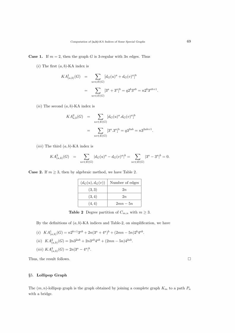
Computation of (a,b)-KA Indices of Some Special Graphs 69
Case 1. If m = 2, then the graph G is 3-regular with 3n edges. Thus
(i) The first (a, b)-KA index is
KA1(a,b)(G) =
∑uv∈E(G)
[dG(u)a + dG(v)a]b
=∑
uv∈E(G)
[3a + 3a]b = q2b3ab = n2b3ab+1.
(ii) The second (a, b)-KA index is
KA2a,b(G) =
∑uv∈E(G)
[dG(u)a.dG(v)a]b
=∑
uv∈E(G)
[3a.3a]b = q32ab = n32ab+1.
(iii) The third (a, b)-KA index is
KA3(a,b)(G) =
∑uv∈E(G)
|dG(u)a − dG(v)a|b =∑
uv∈E(G)
|3a − 3a|b = 0.
Case 2. If m ≥ 3, then by algebraic method, we have Table 2.
(dG(u), dG(v)) Number of edges
(3, 3) 2n
(3, 4) 2n
(4, 4) 2mn− 5n
Table 2 Degree partition of Cm,n with m ≥ 3.
By the definitions of (a, b)-KA indices and Table-2, on simplification, we have
(i) KA1(a,b)(G) = n2b+13ab + 2n(3a + 4a)b + (2mn− 5n)2b4ab.
(ii) KA2(a,b)(G) = 2n32ab + 2n3ab4ab + (2mn− 5n)42ab.
(iii) KA3(a,b)(G) = 2n|3a − 4a|b.
Thus, the result follows. �
§5. Lollipop Graph
The (m,n)-lollipop graph is the graph obtained by joining a complete graph Km to a path Pn
with a bridge.
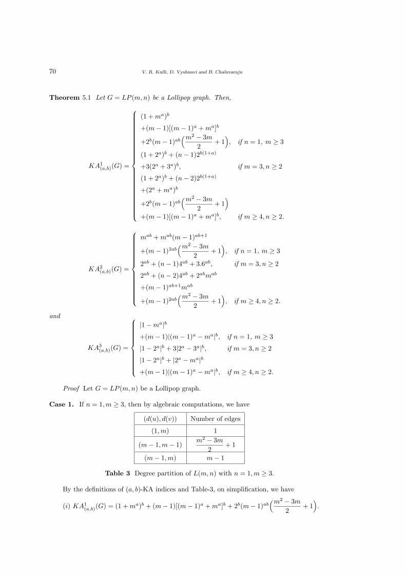
70 V. R. Kulli, D. Vyshnavi and B. Chaluvaraju
Theorem 5.1 Let G = LP (m,n) be a Lollipop graph. Then,
KA1(a,b)(G) =
(1 +ma)b
+(m− 1)[(m− 1)a +ma]b
+2b(m− 1)ab(m2 − 3m
2+ 1), if n = 1, m ≥ 3
(1 + 2a)b + (n− 1)2b(1+a)
+3(2a + 3a)b, if m = 3, n ≥ 2
(1 + 2a)b + (n− 2)2b(1+a)
+(2a +ma)b
+2b(m− 1)ab(m2 − 3m
2+ 1)
+(m− 1)[(m− 1)a +ma]b, if m ≥ 4, n ≥ 2.
KA2(a,b)(G) =
mab +mab(m− 1)ab+1
+(m− 1)2ab(m2 − 3m
2+ 1), if n = 1, m ≥ 3
2ab + (n− 1)4ab + 3.6ab, if m = 3, n ≥ 2
2ab + (n− 2)4ab + 2abmab
+(m− 1)ab+1mab
+(m− 1)2ab(m2 − 3m
2+ 1), if m ≥ 4, n ≥ 2.
and
KA3(a,b)(G) =
|1−ma|b
+(m− 1)|(m− 1)a −ma|b, if n = 1, m ≥ 3
|1− 2a|b + 3|2a − 3a|b, if m = 3, n ≥ 2
|1− 2a|b + |2a −ma|b
+(m− 1)|(m− 1)a −ma|b, if m ≥ 4, n ≥ 2.
Proof Let G = LP (m,n) be a Lollipop graph.
Case 1. If n = 1,m ≥ 3, then by algebraic computations, we have
(d(u), d(v)) Number of edges
(1,m) 1
(m− 1,m− 1)m2 − 3m
2+ 1
(m− 1,m) m− 1
Table 3 Degree partition of L(m,n) with n = 1,m ≥ 3.
By the definitions of (a, b)-KA indices and Table-3, on simplification, we have
(i) KA1(a,b)(G) = (1 +ma)b + (m− 1)[(m− 1)a +ma]b + 2b(m− 1)ab
(m2 − 3m
2+ 1).
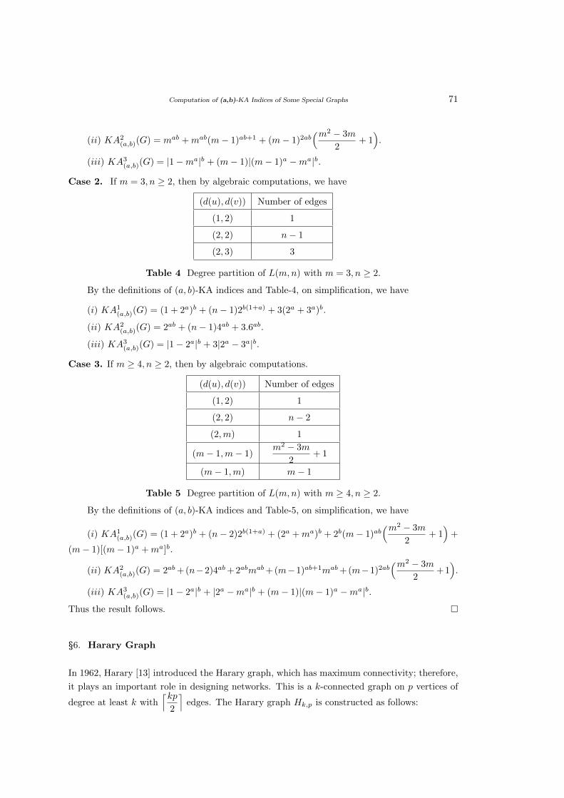
Computation of (a,b)-KA Indices of Some Special Graphs 71
(ii) KA2(a,b)(G) = mab +mab(m− 1)ab+1 + (m− 1)2ab
(m2 − 3m
2+ 1).
(iii) KA3(a,b)(G) = |1−ma|b + (m− 1)|(m− 1)a −ma|b.
Case 2. If m = 3, n ≥ 2, then by algebraic computations, we have
(d(u), d(v)) Number of edges
(1, 2) 1
(2, 2) n− 1
(2, 3) 3
Table 4 Degree partition of L(m,n) with m = 3, n ≥ 2.
By the definitions of (a, b)-KA indices and Table-4, on simplification, we have
(i) KA1(a,b)(G) = (1 + 2a)b + (n− 1)2b(1+a) + 3(2a + 3a)b.
(ii) KA2(a,b)(G) = 2ab + (n− 1)4ab + 3.6ab.
(iii) KA3(a,b)(G) = |1− 2a|b + 3|2a − 3a|b.
Case 3. If m ≥ 4, n ≥ 2, then by algebraic computations.
(d(u), d(v)) Number of edges
(1, 2) 1
(2, 2) n− 2
(2,m) 1
(m− 1,m− 1)m2 − 3m
2+ 1
(m− 1,m) m− 1
Table 5 Degree partition of L(m,n) with m ≥ 4, n ≥ 2.
By the definitions of (a, b)-KA indices and Table-5, on simplification, we have
(i) KA1(a,b)(G) = (1 + 2a)b + (n− 2)2b(1+a) + (2a +ma)b + 2b(m− 1)ab
(m2 − 3m
2+ 1)
+
(m− 1)[(m− 1)a +ma]b.
(ii) KA2(a,b)(G) = 2ab+(n−2)4ab+2abmab+(m−1)ab+1mab+(m−1)2ab
(m2 − 3m
2+1).
(iii) KA3(a,b)(G) = |1− 2a|b + |2a −ma|b + (m− 1)|(m− 1)a −ma|b.
Thus the result follows. �
§6. Harary Graph
In 1962, Harary [13] introduced the Harary graph, which has maximum connectivity; therefore,
it plays an important role in designing networks. This is a k-connected graph on p vertices of
degree at least k with⌈kp
2
⌉edges. The Harary graph Hk,p is constructed as follows:
72 V. R. Kulli, D. Vyshnavi and B. Chaluvaraju
1. k even: Let k = 2r. Then H2r,p is constructed by the vertices 0, 1, . . . , p − 1 and two
vertices i and j are joined if i− r ≤ j ≤ i+ r.
2. k odd, p even. Let k = 2r + 1. Then H2r+1,p is constructed by first drawing H2r,p and
then adding edges joining vertex i to vertex i+ (p2 ) for 1 ≤ i ≤ p2 .
3. k odd, p odd : Let k = 2r+1. Then H2r+1,p is constructed by first drawing H2r,p and then
adding edges joining vertex 0 to vertices (p−1)2 and (p+1)
2 and vertex i to vertex i+ (p+1)2
for 1 ≤ i ≤ (p−1)2 .
Theorem 6.1 Let G = Hk,p be a Harary graph.
(1) If k is even, then
(i) KA1(a,b)(G) =
⌈kp2
⌉2bkab;
(ii) KA2(a,b)(G) =
⌈kp2
⌉k2ab;
(iii) KA3(a,b)(G) = 0.
(2) If k is odd and p is even, then
(i) KA1(a,b)(G) =
⌈kp2
⌉2bkab;
(ii) KA2(a,b)(G) =
⌈kp2
⌉k2ab;
(iii) KA3(a,b)(G) = 0.
(3) If k is odd and p is odd, then
(i) KA1(a,b)(G) =
{⌈kp2
⌉− (k + 1)
}(2bkab) + (k + 1)(ka + (k + 1)a)b;
(ii) KA2(a,b)(G) =
{⌈kp2
⌉− (k + 1)
}(k2ab) + (k + 1)(kab(k + 1)ab);
(iii) KA3(a,b)(G) = (k + 1)|ka − (k + 1)a|b.
Proof Let G = Hk,p be a Harary graph. We have
(1) If k is even, then
(i) The first (a, b)-KA index is
KA1(a,b)(G) =
∑uv∈E(G)
[dG(u)a + dG(v)a]b
=∑
uv∈E(G)
[ka + ka]b = q2bkab =⌈kn
2
⌉2bkab.
(ii) The second (a, b)-KA index is
KA2(a,b)(G) =
∑uv∈E(G)
[dG(u)a.dG(v)a]b
=∑
uv∈E(G)
[ka.ka]b = qk2ab =⌈kn
2
⌉k2ab.
Computation of (a,b)-KA Indices of Some Special Graphs 73
(iii) The third (a, b)-KA index is
KA3(a,b)(G) =
∑uv∈E(G)
|dG(u)a − dG(v)a|b
=∑
uv∈E(G)
|ka − ka|b = 0.
(2) If k is odd and p is even, then
(i) The first (a, b)-KA index is
KA1(a,b)(G) =
∑uv∈E(G)
[dG(u)a + dG(v)a]b
= q2bkab =⌈kn
2
⌉2bkab.
(ii) The second (a, b)-KA index is
KA2(a,b)(G) =
∑uv∈E(G)
[dG(u)a.dG(v)a]b
= qk2ab =⌈kn
2
⌉k2ab.
(iii) The third (a, b)-KA index is
KA3(a,b)(G) =
∑uv∈E(G)
|dG(u)a − dG(v)a|b =∑
uv∈E(G)
|ka − ka|b = 0.
(3) If k is odd and p is odd, then
(i) The first (a, b)-KA index is
KA1(a,b)(G) =
∑uv∈E(G)
[dG(u)a + dG(v)a]b
=
{⌈kp2
⌉− (k + 1)
}(ka + ka)b + (k + 1)[ka + (k + 1)a]b
=
{⌈kp2
⌉− (k + 1)
}(2bkab) + (k + 1)[ka + (k + 1)a]b.
(ii) The second (a, b)-KA index is
KA2(a,b)(G) =
∑uv∈E(G)
[dG(u)a.dG(v)a]b
=
{⌈kp2
⌉− (k + 1)
}(ka.ka)b + (k + 1)[ka.(k + 1)a]b
=
{⌈kp2
⌉− (k + 1)
}(k2ab) + (k + 1)[kab(k + 1)ab].
74 V. R. Kulli, D. Vyshnavi and B. Chaluvaraju
(iii) The third (a, b)-KA index is
KA3(a,b)(G) =
∑uv∈E(G)
|dG(u)a − dG(v)a|b
=
{⌈kp2
⌉− (k + 1)
}|ka − ka|b + (k + 1)|ka − (k + 1)a|b
= (k + 1)|ka − (k + 1)a|b.
Thus, the result follows. �
§7. Conclusions
Being new generalized version of vertex degree based topological indices, the (a, b) KA-indices
lies on the fact that their special cases, for pertinently chosen values of the parameters a and b,
coincide with the vast majority of previously considered topological indices. For the comparative
advantages, applications and in mathematical point of view, few problems are suggested by this
research, among them are the following.
Problem 7.1 Find the extremal values and extremal graphs of the (a, b)-KA indices.
Problem 7.2 Find the values of (a, b)-KA indices for certain classes of chemical graphs and
explore some results towards QSPR / QSAR / QSTR Model.
Problem 7.3 Obtain the relationship between (a, b)-KA indices in terms of other degree/
distance/spectral based topological indices.
Acknowledgement
The authors would like to thank the anonymous reviewers for their valuable comments and
suggestions to improve the quality of the paper.
References
[1] M. O. Albertson, The irregularity of a graph, Ars Comb., 46 (1997), 219–225.
[2] A. Alameri, N. Al-Naggar, M. Al-Rumaima, and M. Alsharafi, Y-index of some graph
operations, J. Appl. Eng. Res., 15(2) (2020), 173–179.
[3] B. Bollobs and P. Erdos, Graphs of extremal weights, Ars Comb., 50 (1998), 225–233.
[4] B. Chaluvaraju, H. S. Boregowda, and I. N. Cangul, Some inequalities for the first general
Zagreb index of graphs and line graphs, Proceedings of the National Academy of Sciences
India Section A-Physical Sciences (2020), doi: 10.1007/s40010-020-00679-9.
[5] B. Furtula and I. Gutman, A forgotten topological index, J. Math. Chem., 53(2015),
1184-1190.
[6] I. Gutman, Degree–based topological indices, Croat. Chem. Acta., 86(2013), 351–361.
Computation of (a,b)-KA Indices of Some Special Graphs 75
[7] I. Gutman, Geometric approach to degree based topological indices, MATCH Commun.
Math. Comput. Chem., 86(1)(2021), 11–16.
[8] I. Gutman, B. Furtula, Z. K. Vukicevic and G. Popivoda, Zagreb indices and coindices,
MATCH Commun. Math. Comput. Chem., 74(2015), 5–16.
[9] S. Ghobadi and M. Ghorbaninejad, On F-polynomial, multiple and hyper F-index of some
molecular graphs, Bull. Math. Sci. Appl., Vol.20(2018), 36–43.
[10] I. Gutman, V.R.Kulli, B. Chaluvaraju and H.S. Boregowda, On Banhatti and Zagreb
Indices, J. Int. Math. Virtual Inst., 7(2017), 53–67.
[11] I. Gutman, M. Togan, A. Yurttas, A. S. Cevik and I. N. Cangul, Inverse Problem for Sigma
Index,MATCH Commun. Math. Comput. Chem., 79 (2018), 491–508.
[12] I. Gutman and N. Trinajstic, Graph Theory and molecular orbitals. Total π-electron energy
of alternant hydrocarbons, Chem. Phys. Lett., 17(1972), 535–538.
[13] F. Harary, The maximum connectivity of a graph, Proc. Nat. Acad. Sci., 48(7)(1962),
1142–1146.
[14] R. Hammack, W. Imrich and S. Klavzar, Hand Book of Product Graph. CRC press, Taylor
& Francis group, LLC (2011).
[15] V. R. Kulli, College Graph Theory, Vishwa Int. Publ., Gulbarga, India (2012).
[16] V. R. Kulli, F-indices of chemical networks, International Journal of Mathematics Archive,
10(3)(2019), 21–30.
[17] V. R. Kulli, Minus F and Square F-indices and their polynomials of certain dendrimers,
Earthline Journal of Mathematical Sciences, 1(2) (2019), 171–185.
[18] V. R. Kulli, Computation of minus F-indices and their polynomials of titania nanotubes,
Annals of Pure and Applied Mathematics, 22(2) (2020), 137–142.
[19] V. R. Kulli, Computation of some minus indices of titania nanotubes, International Journal
of Current Research in Science and Technology, 4(12) (2018), 9–13.
[20] V. R. Kulli, Graph indices, in Hand Book of Research on Advanced Applications of Graph
Theory in Modern Society, M. Pal. S. Samanta and A. Pal, (eds.) IGI Global, USA, 2019,
66–91.
[21] V. R. Kulli, The (a, b) -KA indices of polycyclic aromatic hydrocarbons and benzenoid
systems, International Journal of Mathematical Trends and Technology, 65(2019), 115–
120.
[22] V. R. Kulli, Nirmala index, International Journal of Mathematical Trends and Technology,
67(3)(2021), 8–12.
[23] V. R. Kulli, Dharwad index, International Journal of Engineering Sciences and Research
Technology, 10(4)(2021), 17–21.
[24] V. R. Kulli and I. Gutmann, (a, b) - KA indices of Benzenoid systems and phenylenes: The
general case, International Journal of Mathematics Trends and Technology, 67(1)(2021),
17–20.
[25] V.Lokesha, K.Z.Yasmeen, B. Chaluvaraju and T. Deepika, Computation of misbalance
type degree indices of certain classes of derived graph, International J. Math. Combin.,
3(2019), 61–69.
76 V. R. Kulli, D. Vyshnavi and B. Chaluvaraju
[26] X. Li and J. Zheng, A unified approach to the extremal trees for different indices, Commun.
Math. Comput. Chem., 54(1)(2005), 195–208.
[27] K. Pattabiraman amd M. Vijayaragavan, Edge a-Zagreb indices and its coindices of trans-
formation graphs, Elec. Notes in Disc. Maths., 63(2017), 251–269.
[28] M. Randic, On characterization of molecular branching, J Am Chem Soc., 97(1975), 6609–
6615.
[29] P. S. Ranjini, V. Lokesha and A. Usha, Relation between phenylene and hexagonal squeeze
using harmonic index, Int. J. Graph Theory, 1(2013), 116–121.
[30] V. Shigehalli and R. Kanabur, Computing degree-based topological indices of polyhex
nanotubes, Journal of Mathematical Nanoscience, 6(2016), 47–55.
[31] G. H. Shirdel, H. Rezapour and A. M. Sayadi, The hyper–Zagreb index of graph operations,
Iran. J. Math. Chem., 4(2)(2013), 213–220.
[32] R. Todeschini and V. Consonni, Molecular Descriptors for Chemoinformatics, Wiley–VCH,
Weinheim (2009).
[33] D. Vukicevic and M. Gasperov, Bond additive modeling 1. Adriatic indices, Croat. Chem.
Acta, 83(2010), 243–260.
[34] G. Wei, M. R. Farahani and M. K. Siddiqui, On the first and second Zagreb and first and
second hyper-Zagreb indices of carbon nanocones CNCk[n], J. Comput. Theor. Nanosci.,
13(2016), 7475–7482.
[35] B. Zhou and N. Trinajstic, On a novel connectivity index, J Math.Chem., 46(2009), 1252–
1270.
International J.Math. Combin. Vol.3(2021), 77-85
The Signed Product Cordial for
Corona Between Paths and Fourth Power of Cycles
Amani Elrayes1, Elsayed Badr2, Ashraf Elrokh3 and Aya Rabie4
1. Institute of National Planning, Egypt
2. Scientific Computing Department, Faculty of Computers and Informatics, Benha University, Benha, Egypt
3. Department of Math, University of Menoyfia, Egypt
4. Institute of National Planning, Egypt
E-mail: [email protected], [email protected], [email protected], [email protected]
Abstract: A graph G = (V,E) is called signed product cordial if it is possible to label the
vertex by the function f : V → {−1, 1} and label the edges by f∗ : E → {−1, 1}, where
f∗(uv) = f(u).f(v), u, v ∈ V so that |v−1 − v1| 6 1 and |e−1 − e1| 6 1. In this paper,some
new results on signed product cordial labeling are proposed. The necessary and sufficient
conditions of signed product cordial for corona between paths and fourth power of cycles are
presented.
Key Words: Corona graph, fourth power, second power, signed product cordial graph,
Smarandachely signed product cordial labeling.
AMS(2010): 05C22.
§1. Introduction
The graph theory is a mathematical subfield of discrete mathematics. One area of graph theory
of considerable recent research is that of graph labeling. The concept of graph labeling was
introduced during the sixties’ of the last century by Rosa [14]. Labeling methods are used for a
wide range of applications in different subjects including coding theory, computer science and
communication networks. Yegnanarayanan [16] explores some of the interesting applications of
graph labeling With advancement in technology the occurrence of more complex networking
system is seen to have emerged. Many researches have been working with different types of
labeling graphs [5,8,11]. In 1954 Harray introduced S-cordiality [12]. An excellent reference
for this purpose is the survey written by Gallian [9]. The original concept of cordial graphs
is due to Cahit[6]. Cordial Labeling finds its application in Automated Routing algorithms,
Communications relevant Adhoc Networks and many others[10].
For more details about the graph labeling, the reader can refer to [2-4,13]. We will give
brief summary of definitions which are useful for the present investigations.
Definition 1.1([15]) If the vertices of the graph are assigned values subject to certain conditions
is known as graph labeling. Following three are the common features of any graph labeling
1Received July 23, 2021, Accepted September 4, 2021.
78 Amani Elrayes, Elsayed Badr, Ashraf Elrokh and Aya Rabie
problem:
(1) a set of numbers from which vertex labels are assigned;
(2) a rule that assigns a value to each edge;
(3) a condition that these values must satisfy.
The present work is targeted to discuss one such labeling known as signed product cordial
labeling defined as follows:
Definition 1.2 Let G = (V,E) be a graph and let f : V → {−1, 1} be a labeling of its vertices,
and let the induced edge labeling f∗ : E → {−1, 1} be given by f∗(e) = (f(u).f(v)), where
e = uv and u, v ∈ V . Let v−1 and v1 be the numbers of vertices that are labeled by −1 and 1,
respectively, and let e−1 and e1 be the corresponding numbers of edges. Such a labeling is called
signed product cordial if both |v−1 − v1| 6 1 and |e−1 − e1| 6 1 hold. On the other hand, if
|v−1 − v1| ≥ 2 or |e−1 − e1| ≥ 2, such a labeling is called Smarandachely signed product cordial
labeling.
The concept of signed product cordial labeling was introduced by Baskar Babujee [1].
Definition 1.3 The corona G1
⊙G2 of two graphs G1 (with n1 vertices, m1 edges) and G2
(with n2 vertices, m2 edges) is defined as the graph obtained by taking one copy of G1 and copies
of G2, and then joining the ith vertex of G1 with an edge to every vertex in the ith copy of G2.
Definition 1.4 The fourth power of a paths Pn, denoted by P 4n , is Pn
⋃J , where J is the set
of all edges of the form edges vivj such that 2 ≤ d(vivj) ≤ 4 and i < j where d(vivj) is the
shortest distance from vi to vj.
§2. Terminologies and Notations
A path with m vertices and m − 1 edges is denoted by Pm. Also, a cycle with n vertices
and n edges, denoted by Cn, and its fourth power C4n has n vertices and 4n − 9 edges.
We let L4r denote the labeling (−1)211 (−1)211 · · · (−1)211 (repeated r-times), Let L′4r de-
note the labeling (−1)11(−1) (−1)11(−1) · · · (−1)11(−1) (repeated r-times). The labeling
11(−1)2 11(−1)2 · · · 11(−1)2 (repeated r-times) and labeling 1(−1)21 1(−1)21· · · 1(−1)21 (re-
peated r-times) are written S4r and S′4r. Let Mr denote the labeling (−1)1 (−1)1 · · · (−1)1,
zero-one repeated rtimes if r is even and (−1)1 (−1)1 · · · (−1)1(−1) if r is odd; for exam-
ple, M6 = (−1)1(−1)1(−1)1 and M5 = (−1)1(−1)1(−1). We let M ′r denote the labeling
1(−1)1(−1) · · · 1(−1).
Sometimes, we modify the labeling Mr or M ′r by adding symbols at one end or the other
(or both). Also, L4r (or L′4r ) with extra labeling from right or left (or both sides). If L is
a labeling for a path pm and M is a labeling for fourth power of path Cn, then we use the
notation [L;M ] to represent the labeling of the corona Pm⊙C4n. Additional notation that we
use is the following: for a given labeling of the corona Pm⊙C4n, we let vi and ei (for i = −1, 1)
be the numbers of vertices and edges, respectively, that are labeled by i of the corona Pm⊙C4n,
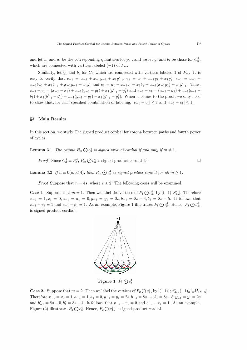
The Signed Product Cordial for Corona Between Paths and Fourth Power of Cycles 79
and let xi and ai be the corresponding quantities for pm, and we let yi and bi be those for C4n,
which are connected with vertices labeled (−1) of Pm.
Similarly, let y′i and b′i for C4n which are connected with vertices labeled 1 of Pm. It is
easy to verify that v−1 = x−1 + x−1y−1 + x1y′−1, v1 = x1 + x−1y1 + x1y
′1, e−1 = a−1 +
x−1b−1 + x1b′−1 + x−1y−1 + x1y
′1 and e1 = a1 + x−1b1 + x1b
′1 + x−1(x−1y1) + x1y
′−1. Thus,
v−1 − v1 = (x−1 − x1) + x−1(y−1 − y1) + x1(y′−1 − y′1) and e−1 − e1 = (a−1 − a1) + x−1(b−1 −b1) + x1(b′−1 − b′1) + x−1(y−1 − y1)− x1(y′−1 − y′1). When it comes to the proof, we only need
to show that, for each specified combination of labeling, |v−1 − v1| ≤ 1 and |e−1 − e1| ≤ 1.
§3. Main Results
In this section, we study The signed product cordial for corona between paths and fourth power
of cycles.
Lemma 3.1 The corona Pm⊙c43 is signed product cordial if and only if m 6= 1.
Proof Since C43 ≡ P 4
3 , Pm⊙c43 is signed product cordial [9]. �
Lemma 3.2 If n ≡ 0(mod 4), then Pm⊙c4n is signed product cordial for all m ≥ 1.
Proof Suppose that n = 4s, where s ≥ 2. The following cases will be examined.
Case 1. Suppose that m = 1. Then we label the vertices of P1
⊙c44s by [(−1);S′4s]. Therefore
x−1 = 1, x1 = 0, a−1 = a1 = 0, y−1 = y1 = 2s, b−1 = 8s − 4, b1 = 8s − 5. It follows that
v−1 − v1 = 1 and e−1 − e1 = 1. As an example, Figure 1 illustrates P1
⊙c48. Hence, P1
⊙c44s
is signed product cordial.
Figure 1 P1
⊙c48
Case 2. Suppose thatm = 2. Then we label the vertices of P2
⊙c44s by [(−1)1;S′4s, (−1)313M4S−6].
Therefore x−1 = x1 = 1, a−1 = 1, a1 = 0, y−1 = y1 = 2s, b−1 = 8s−4, b1 = 8s−5, y′−1 = y′1 = 2s
and b′−1 = 8s− 5, b′1 = 8s− 4. It follows that v−1 − v1 = 0 and e−1 − e1 = 1. As an example,
Figure (2) illustrates P2
⊙c48. Hence, P2
⊙c44s is signed product cordial.
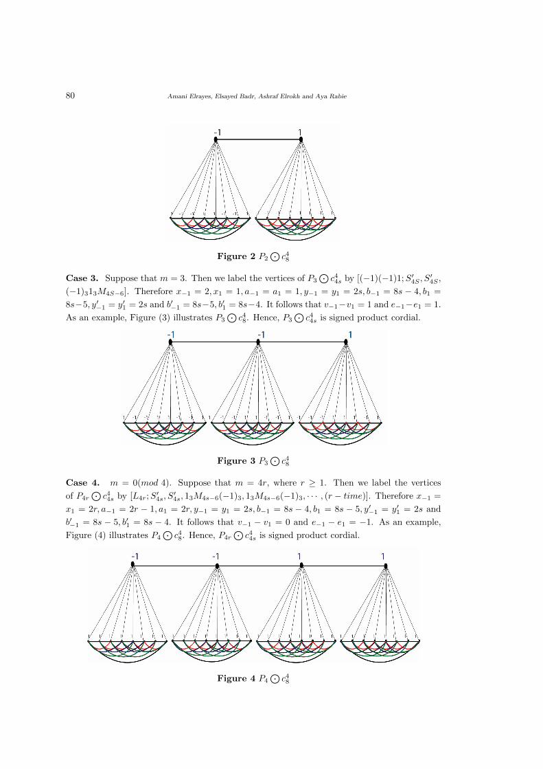
80 Amani Elrayes, Elsayed Badr, Ashraf Elrokh and Aya Rabie
Figure 2 P2
⊙c48
Case 3. Suppose that m = 3. Then we label the vertices of P3
⊙c44s by [(−1)(−1)1;S′4S , S
′4S ,
(−1)313M4S−6]. Therefore x−1 = 2, x1 = 1, a−1 = a1 = 1, y−1 = y1 = 2s, b−1 = 8s − 4, b1 =
8s−5, y′−1 = y′1 = 2s and b′−1 = 8s−5, b′1 = 8s−4. It follows that v−1−v1 = 1 and e−1−e1 = 1.
As an example, Figure (3) illustrates P3
⊙c48. Hence, P3
⊙c44s is signed product cordial.
Figure 3 P3
⊙c48
Case 4. m = 0(mod 4). Suppose that m = 4r, where r ≥ 1. Then we label the vertices
of P4r
⊙c44s by [L4r;S
′4s, S
′4s, 13M4s−6(−1)3, 13M4s−6(−1)3, · · · , (r − time)]. Therefore x−1 =
x1 = 2r, a−1 = 2r − 1, a1 = 2r, y−1 = y1 = 2s, b−1 = 8s − 4, b1 = 8s − 5, y′−1 = y′1 = 2s and
b′−1 = 8s − 5, b′1 = 8s − 4. It follows that v−1 − v1 = 0 and e−1 − e1 = −1. As an example,
Figure (4) illustrates P4
⊙c48. Hence, P4r
⊙c44s is signed product cordial.
Figure 4 P4
⊙c48
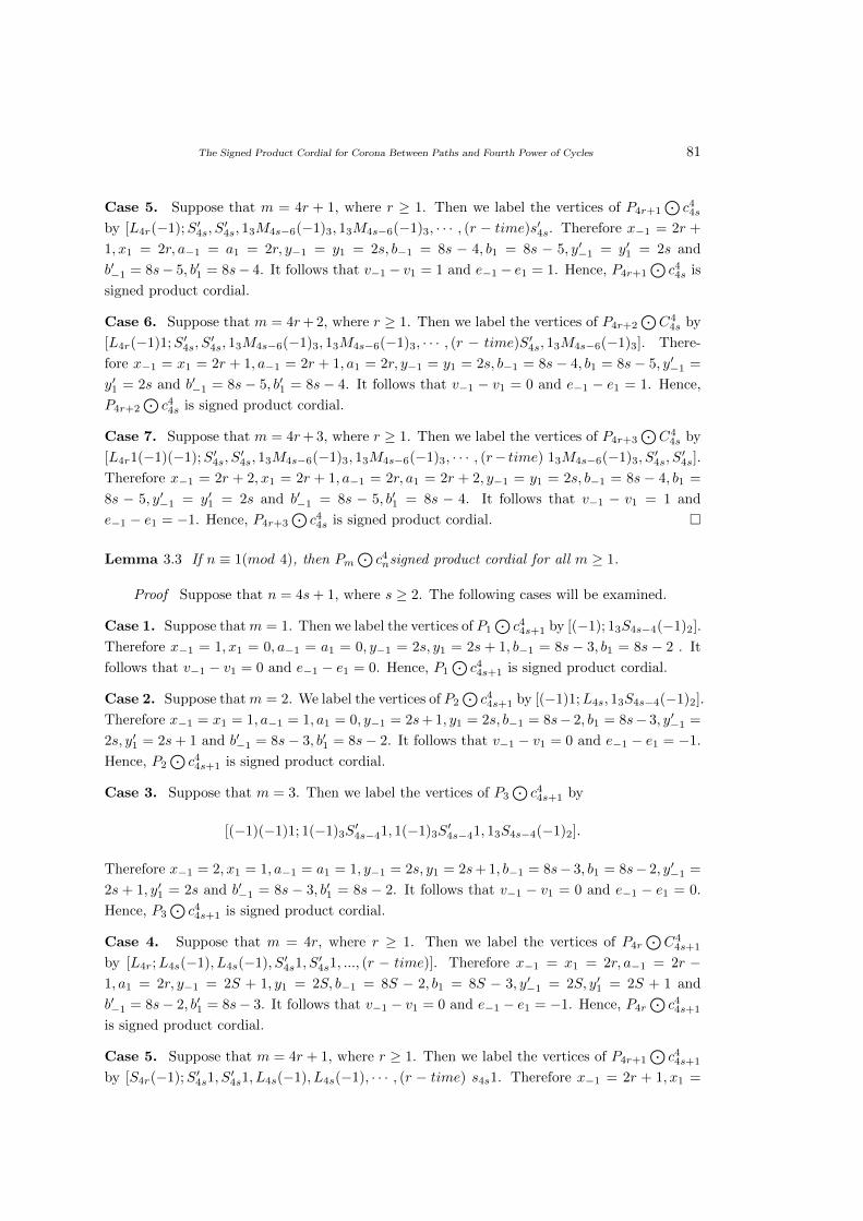
The Signed Product Cordial for Corona Between Paths and Fourth Power of Cycles 81
Case 5. Suppose that m = 4r + 1, where r ≥ 1. Then we label the vertices of P4r+1
⊙c44s
by [L4r(−1);S′4s, S′4s, 13M4s−6(−1)3, 13M4s−6(−1)3, · · · , (r − time)s′4s. Therefore x−1 = 2r +
1, x1 = 2r, a−1 = a1 = 2r, y−1 = y1 = 2s, b−1 = 8s − 4, b1 = 8s − 5, y′−1 = y′1 = 2s and
b′−1 = 8s− 5, b′1 = 8s− 4. It follows that v−1 − v1 = 1 and e−1 − e1 = 1. Hence, P4r+1
⊙c44s is
signed product cordial.
Case 6. Suppose that m = 4r+ 2, where r ≥ 1. Then we label the vertices of P4r+2
⊙C4
4s by
[L4r(−1)1;S′4s, S′4s, 13M4s−6(−1)3, 13M4s−6(−1)3, · · · , (r − time)S′4s, 13M4s−6(−1)3]. There-
fore x−1 = x1 = 2r + 1, a−1 = 2r + 1, a1 = 2r, y−1 = y1 = 2s, b−1 = 8s− 4, b1 = 8s− 5, y′−1 =
y′1 = 2s and b′−1 = 8s − 5, b′1 = 8s − 4. It follows that v−1 − v1 = 0 and e−1 − e1 = 1. Hence,
P4r+2
⊙c44s is signed product cordial.
Case 7. Suppose that m = 4r+ 3, where r ≥ 1. Then we label the vertices of P4r+3
⊙C4
4s by
[L4r1(−1)(−1);S′4s, S′4s, 13M4s−6(−1)3, 13M4s−6(−1)3, · · · , (r− time) 13M4s−6(−1)3, S
′4s, S
′4s].
Therefore x−1 = 2r + 2, x1 = 2r + 1, a−1 = 2r, a1 = 2r + 2, y−1 = y1 = 2s, b−1 = 8s − 4, b1 =
8s − 5, y′−1 = y′1 = 2s and b′−1 = 8s − 5, b′1 = 8s − 4. It follows that v−1 − v1 = 1 and
e−1 − e1 = −1. Hence, P4r+3
⊙c44s is signed product cordial. �
Lemma 3.3 If n ≡ 1(mod 4), then Pm⊙c4nsigned product cordial for all m ≥ 1.
Proof Suppose that n = 4s+ 1, where s ≥ 2. The following cases will be examined.
Case 1. Suppose thatm = 1. Then we label the vertices of P1
⊙c44s+1 by [(−1); 13S4s−4(−1)2].
Therefore x−1 = 1, x1 = 0, a−1 = a1 = 0, y−1 = 2s, y1 = 2s + 1, b−1 = 8s − 3, b1 = 8s − 2 . It
follows that v−1 − v1 = 0 and e−1 − e1 = 0. Hence, P1
⊙c44s+1 is signed product cordial.
Case 2. Suppose thatm = 2. We label the vertices of P2
⊙c44s+1 by [(−1)1;L4s, 13S4s−4(−1)2].
Therefore x−1 = x1 = 1, a−1 = 1, a1 = 0, y−1 = 2s+ 1, y1 = 2s, b−1 = 8s− 2, b1 = 8s− 3, y′−1 =
2s, y′1 = 2s+ 1 and b′−1 = 8s− 3, b′1 = 8s− 2. It follows that v−1 − v1 = 0 and e−1 − e1 = −1.
Hence, P2
⊙c44s+1 is signed product cordial.
Case 3. Suppose that m = 3. Then we label the vertices of P3
⊙c44s+1 by
[(−1)(−1)1; 1(−1)3S′4s−41, 1(−1)3S
′4s−41, 13S4s−4(−1)2].
Therefore x−1 = 2, x1 = 1, a−1 = a1 = 1, y−1 = 2s, y1 = 2s+ 1, b−1 = 8s− 3, b1 = 8s− 2, y′−1 =
2s + 1, y′1 = 2s and b′−1 = 8s − 3, b′1 = 8s − 2. It follows that v−1 − v1 = 0 and e−1 − e1 = 0.
Hence, P3
⊙c44s+1 is signed product cordial.
Case 4. Suppose that m = 4r, where r ≥ 1. Then we label the vertices of P4r
⊙C4
4s+1
by [L4r;L4s(−1), L4s(−1), S′4s1, S′4s1, ..., (r − time)]. Therefore x−1 = x1 = 2r, a−1 = 2r −
1, a1 = 2r, y−1 = 2S + 1, y1 = 2S, b−1 = 8S − 2, b1 = 8S − 3, y′−1 = 2S, y′1 = 2S + 1 and
b′−1 = 8s− 2, b′1 = 8s− 3. It follows that v−1 − v1 = 0 and e−1 − e1 = −1. Hence, P4r
⊙c44s+1
is signed product cordial.
Case 5. Suppose that m = 4r + 1, where r ≥ 1. Then we label the vertices of P4r+1
⊙c44s+1
by [S4r(−1);S′4s1, S′4s1, L4s(−1), L4s(−1), · · · , (r − time) s4s1. Therefore x−1 = 2r + 1, x1 =
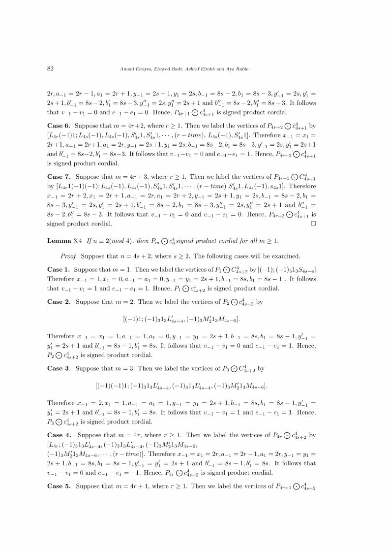
82 Amani Elrayes, Elsayed Badr, Ashraf Elrokh and Aya Rabie
2r, a−1 = 2r − 1, a1 = 2r + 1, y−1 = 2s + 1, y1 = 2s, b−1 = 8s − 2, b1 = 8s − 3, y′−1 = 2s, y′1 =
2s+ 1, b′−1 = 8s− 2, b′1 = 8s− 3, y′′−1 = 2s, y′′1 = 2s+ 1 and b′′−1 = 8s− 2, b′′1 = 8s− 3. It follows
that v−1 − v1 = 0 and e−1 − e1 = 0. Hence, P4r+1
⊙c44s+1 is signed product cordial.
Case 6. Suppose that m = 4r+2, where r ≥ 1. Then we label the vertices of P4r+2
⊙c44s+1 by
[L4r(−1)1;L4s(−1), L4s(−1), S′4s1, S′4s1, · · · , (r − time), L4s(−1), S′4s1]. Therefore x−1 = x1 =
2r+1, a−1 = 2r+1, a1 = 2r, y−1 = 2s+1, y1 = 2s, b−1 = 8s−2, b1 = 8s−3, y′−1 = 2s, y′1 = 2s+1
and b′−1 = 8s−2, b′1 = 8s−3. It follows that v−1−v1 = 0 and e−1−e1 = 1. Hence, P4r+2
⊙c44s+1
is signed product cordial.
Case 7. Suppose that m = 4r+ 3, where r ≥ 1. Then we label the vertices of P4r+3
⊙C4
4s+1
by [L4r1(−1)(−1);L4s(−1), L4s(−1), S′4s1, S′4s1, · · · , (r − time) S′4s1, L4s(−1), s4s1]. Therefore
x−1 = 2r + 2, x1 = 2r + 1, a−1 = 2r, a1 = 2r + 2, y−1 = 2s + 1, y1 = 2s, b−1 = 8s − 2, b1 =
8s − 3, y′−1 = 2s, y′1 = 2s + 1, b′−1 = 8s − 2, b1 = 8s − 3, y′′−1 = 2s, y′′1 = 2s + 1 and b′′−1 =
8s − 2, b′′1 = 8s − 3. It follows that v−1 − v1 = 0 and e−1 − e1 = 0. Hence, P4r+3
⊙c44s+1 is
signed product cordial. �
Lemma 3.4 If n ≡ 2(mod 4), then Pm⊙c4nsigned product cordial for all m ≥ 1.
Proof Suppose that n = 4s+ 2, where s ≥ 2. The following cases will be examined.
Case 1. Suppose thatm = 1. Then we label the vertices of P1
⊙C4
4s+2 by [(−1); (−1)313S4s−4].
Therefore x−1 = 1, x1 = 0, a−1 = a1 = 0, y−1 = y1 = 2s + 1, b−1 = 8s, b1 = 8s − 1 . It follows
that v−1 − v1 = 1 and e−1 − e1 = 1. Hence, P1
⊙c44s+2 is signed product cordial.
Case 2. Suppose that m = 2. Then we label the vertices of P2
⊙c44s+2 by
[(−1)1; (−1)313L′4s−4, (−1)3M
′213M4s−6].
Therefore x−1 = x1 = 1, a−1 = 1, a1 = 0, y−1 = y1 = 2s + 1, b−1 = 8s, b1 = 8s − 1, y′−1 =
y′1 = 2s + 1 and b′−1 = 8s − 1, b′1 = 8s. It follows that v−1 − v1 = 0 and e−1 − e1 = 1. Hence,
P2
⊙c44s+2 is signed product cordial.
Case 3. Suppose that m = 3. Then we label the vertices of P3
⊙C4
4s+2 by
[(−1)(−1)1; (−1)313L′4s−4, (−1)313L
′4s−4, (−1)3M
′213M4s−6].
Therefore x−1 = 2, x1 = 1, a−1 = a1 = 1, y−1 = y1 = 2s + 1, b−1 = 8s, b1 = 8s − 1, y′−1 =
y′1 = 2s + 1 and b′−1 = 8s − 1, b′1 = 8s. It follows that v−1 − v1 = 1 and e−1 − e1 = 1. Hence,
P3
⊙c44s+2 is signed product cordial.
Case 4. Suppose that m = 4r, where r ≥ 1. Then we label the vertices of P4r
⊙c44s+2 by
[L4r; (−1)313L′4s−4, (−1)313L
′4s−4, (−1)3M
′213M4s−6,
(−1)3M′213M4s−6, · · · , (r− time)]. Therefore x−1 = x1 = 2r, a−1 = 2r− 1, a1 = 2r, y−1 = y1 =
2s + 1, b−1 = 8s, b1 = 8s − 1, y′−1 = y′1 = 2s + 1 and b′−1 = 8s − 1, b′1 = 8s. It follows that
v−1 − v1 = 0 and e−1 − e1 = −1. Hence, P4r
⊙c44s+2 is signed product cordial.
Case 5. Suppose that m = 4r + 1, where r ≥ 1. Then we label the vertices of P4r+1
⊙c44s+2
The Signed Product Cordial for Corona Between Paths and Fourth Power of Cycles 83
by [L4r(−1); (−1)313L′4s−4, (−1)313L
′4s−4, (−1)3M
′213 M4s−6, (−1)3M
′213M4s−6, · · · , (r−time)
(−1)313L′4s−4. Therefore x−1 = 2r+1, x1 = 2r, a−1 = a1 = 2r, y−1 = y1 = 2s+1, b−1 = 8s, b1 =
8s−1, y′−1 = y′1 = 2s+1 and b′−1 = 8s−1, b′1 = 8s. It follows that v−1−v1 = 1 and e−1−e1 = 1.
Hence, P4r+1
⊙c44s+2 is signed product cordial.
Case 6. Suppose that m = 4r + 2, where r ≥ 1. Then we label the vertices of P4r+2
⊙c44s+2
by
[L4r(−1)1; (−1)313L′4s−4, (−1)313L
′4s−4, (−1)3M
′213M4s−6, (−1)3M
′213M4s−6,
· · · , (r − time)(−1)313L′4s−4, (−1)3M
′213M4s−6].
Therefore x−1 = x1 = 2r + 1, a−1 = 2r + 1, a1 = 2r, y−1 = y1 = 2s + 1, b−1 = 8s, b1 =
8s − 1, y′−1 = y′1 = 2s + 1 and b′−1 = 8s − 1, b′1 = 8s. It follows that v−1 − v1 = 0 and
e−1 − e1 = 1. Hence, P4r+2
⊙c44s+2 is signed product cordial.
Case 7. Suppose that m = 4r + 3, where r ≥ 1. Then we label the vertices of P4r+3
⊙c44s+2
by [L4r1(−1)(−1); (−1)313L′4s−4, (−1)313L
′4s−4, (−1)3M
′213 M4s−6, (−1)3M
′213M4s−6, · · · , (r−
time), (−1)3M′213M4s−6, (−1)313L
′4s−4, (−1)313L
′4s−4]. Therefore x−1 = 2r + 2, x1 = 2r +
1, a−1 = 2r, a1 = 2r + 2, y−1 = y1 = 2s + 1, b−1 = 8s, b1 = 8s − 1, y′−1 = y′1 = 2s + 1 and
b′−1 = 8s − 1, b′1 = 8s. It follows that v−1 − v1 = 1 and e−1 − e1 = −1. Hence, P4r+3
⊙c44s+2
is signed product cordial. �
Lemma 3.5 If n ≡ 3(mod 4), then Pm⊙c4nsigned product cordial for all m ≥ 1.
Proof Suppose that n = 4s+ 3, where s ≥ 2. The following cases will be examined.
Case 1. Suppose thatm = 2. We label the vertices of P2
⊙c44s+3 by [(−1)1;M4s+3, S
′4s1(−1)1].
Therefore x−1 = x1 = 1, a−1 = 1, a1 = 0, y−1 = 2s + 2, y1 = 2s + 1, b−1 = 8s + 2, b1 =
8s+ 1, y′−1 = 2s+ 1, y′1 = 2s+ 2 and b′−1 = 8s+ 2, b′1 = 8s+ 1. It follows that v−1− v1 = 0 and
e−1 − e1 = 1. Hence, P2
⊙c44s+3 is signed product cordial.
Case 2. Suppose that m = 4r, where r ≥ 1. Then we label the vertices of P4r
⊙C4
4s+3
by [L4r;M4s+3,M4s+3, S′4s1(−1)1, S′4s1(−1)1, ..., (r − time)]. Therefore x−1 = x1 = 2r, a−1 =
2r−1, a1 = 2r, y−1 = 2s+2, y1 = 2s+1, b−1 = 8s+2, b1 = 8s+1, y′−1 = 2s+1, y′1 = 2s+2 and
b′−1 = 8s+ 2, b′1 = 8s+ 1. It follows that v−1 − v1 = 0 and e−1 − e1 = −1. Hence, P4r
⊙c44s+3
is signed product cordial.
Case 3. Suppose that m = 4r + 1, where r ≥ 1. Then we label the vertices of P4r+1
⊙c44s+3
by [S4r(−1);S′4s1(−1)1, S′4s1(−1)1,M4s+3,M4s+3, , · · · , (r−time),s′4s1(−1)1. Therefore x−1 =
2r+1, x1 = 2r, a−1 = 2r−1, a1 = 2r+1, y−1 = 2s+2, y1 = 2s+1, b−1 = 8s+2, b1 = 8s+1, y′−1 =
2s+1, y′1 = 2s+2, b′−1 = 8s+2, b′1 = 8s+1, y′′−1 = 2s+1, y′1 = 2s+2 and b′′−1 = 8s+2, b′′1 = 8s+1.
It follows that v−1 − v1 = 0 and e−1 − e1 = 0. Hence, P4r+1
⊙c44s+3 is signed product cordial.
Case 4. Suppose that m = 4r+2, where r ≥ 1. Then we label the vertices of P4r+2
⊙c44s+3 by
[L4r(−1)1;M4s+3,M4s+3, S′4s1(−1)1, S′4s1(−1)1, · · · , (r− time), M4s+3, S
′4s1(−1)1]. Therefore
x−1 = x1 = 2r + 1, a−1 = 2r + 1, a1 = 2r, y−1 = 2s + 2, y1 = 2s + 1, b−1 = 8s + 2, b1 =
8s+ 1, y′−1 = 2s+ 1, y′1 = 2s+ 2 and b′−1 = 8s+ 2, b′1 = 8s+ 1. It follows that v−1− v1 = 0 and
84 Amani Elrayes, Elsayed Badr, Ashraf Elrokh and Aya Rabie
e−1 − e1 = 1. Hence, P4r+2
⊙c44s+3 is signed product cordial.
Case 5. Suppose that m = 4r + 3, where r ≥ 1. Then we label the vertices of P4r+3
⊙c44s+3
by
[L4r1(−1)(−1);M4s+3,M4s+3, S′4s1(−1)1, S′4s1(−1)1, · · · , (r − time), S′4s1(−1)1,M4s+3, S4s1(−1)1].
Therefore x−1 = 2r + 2, x1 = 2r + 1, a−1 = 2r, a1 = 2r + 2, y−1 = 2s + 2, y1 = 2s + 1, b−1 =
8s+ 2, b1 = 8s+ 1, y′−1 = 2s+ 1, y′1 = 2s+ 2, b′−1 = 8s+ 2, b1 = 8s+ 1, y′′−1 = 2s+ 1, y′′1 = 2s+ 2
and b′′−1 = 8s + 2, b′′1 = 8s + 1. It follows that v−1 − v1 = 0 and e−1 − e1 = 0. Hence,
P4r+3
⊙c44s+3 is signed product cordial. �
As a consequence of all lemmas mentioned above we conclude that the corona between
paths and fourth power of cycles is signed product cordial for all m,n if and only if m ≥ 1,
n ≥ 7 except (m,n) = (1, 7) or (3, 7) and also if n = 3 for all m 6= 1, i.e., the conclusion
following.
Theorem 3.5 Pm⊙c4n is signed product cordial for all m,n if and only if m ≥ 1, n ≥ 7 except
(m,n) = (1, 7) or (3, 7).
In [5] it is proved that the corona Pm⊙c43 is signed product cordial if and only if m 6= 1.
Certainly, we get a general result on the signed product cordial of the corona between paths
and fourth power of cycles in this paper.
Acknowledgement
The authors are thankful to the anonymous referee for useful suggestions and valuable com-
ments.
References
[1] Babujee J. B. and Loganathan S., On signed product cordial labeling, Scientific Research
Journal on Applied Mathematics, 2(2011), 1525-1530.
[2] Badr E., Almotairi S, Elrokh A, Abdel-Hady A and Almutairi B, An integer linear pro-
gramming model for solving radio mean labeling problem, IEEE Access, Vol.8 (2020),
162343-162349, doi: 10.1109/ACCESS.2020.3021896.
[3] Badr E. M. and Moussa M. I., An upper bound of radio k-coloring problem and its integer
linear programming model, Wireless and Networks (published online:18 March 2019).
[4] Badr E. M., Moussa M. I. and Kathiresan K,: Crown graphs and subdivision of ladders are
odd graceful, International Journal of Computer Mathematics, 88:17(2011), 3570-3576.
[5] Cahit I., Cordial graphs: A weaker version of graceful and harmonious graphs, Ars Com-
binatoria, 23(1987), 201-207.
[6] Cahit I., On cordial and 3-eqtitable labeling of graphs, Utiliuies Math.,(1990)
[7] Diab A .T., On cordial labeling of the second power of paths with other graphs, Ars
Combinatoria, 97A(2010), 327-343.
The Signed Product Cordial for Corona Between Paths and Fourth Power of Cycles 85
[8] Elrokh A. and Rabie A., The signed product cordial for corona of paths and fourth power
of paths, International Journal of Mathematical Combinatorics, Vol.4(2019), 102-111.
[9] Gallian J. A., A dynamic survey of graph labeling, The electronic Journal of Combinatorics,
17(2010), DS6 November.
[10] Ghosh S., Mohanty S. and Pal A., Cordial labeling of Cartesian product between two
balanced bipartite graphs, Journal of Informatics and Mathematical Sciences, (2019), 179-
193.
[11] Graham R. L. and Sloane N. J., On additive bases and harmonious graphs, SIAM J. Alg.
Discrete Math., 1(1980), 382-404.
[12] Harray F., On the notion of a signed graph, Michigan Math. J, (1953-1954), 143-146.
[13] Moussa M.I. and Badr E. M., Ladder and subdivision of ladder graphs with pendant edges
are odd graceful, Journal on Application of Graph Theory in Wireless Ad hoc Networks
and Sensor Networks (GRAPHS-HOC), Vol.8, No.1(2016), March 2016.
[14] Rosa A., On certain valuations of the vertices of a graph, Theory of Graphs (Internat
Symposium, Rome, July 1966), Gordon and Breach, N.Y. and Dunod Paris, (1967), 349-
355.
[15] Seoud M. A., Diab A. T. and Elsahawi E. A., On strongly-C harmonious, relatively prime,
odd graceful and cordial graphs, Proc. Math. Phys. Soc. Egypt, No.73(1998), 33-55.
[16] Yegnanarayanan V., Some interesting applications of graph labellings, Journal of Mathe-
matical and Computational Science, 2(5)(2012), 15-22.
International J.Math. Combin. Vol.3(2021), 86-97
Roman Domination Polynomial of Cycles
Deepak G.1, Anwar Alwardi2 and Indiramma M. H.3
1,3.Sri Venkateshwara college of Engineering, Bangalore 562157, India
2.Department of Mathematics, Aden University, Aden, Yemen
Abstract: A Roman dominating function on a graph G = (V,E) is a function f : V (G)→{0, 1, 2} satisfying the condition that every vertex u for which f(u) = 0 is adjacent to at
least one vertex v for which f(v) = 2. The weight of a Roman dominating function is the
value
W (f(V )) =∑
u∈V (G)
f(u).
The minimum weight of a Roman dominating function on a graph G is called the Roman
domination number of G and is denoted by γR(G). In [9], we have introduced and established
the study of the Roman domination polynomial of graphs and obtained some important
properties about the polynomial and we have computed the polynomial for some specific
graphs and graph operations. In this paper, we study the Roman domination polynomial
of a cycle Cn on n vertices. Exact formula for the polynomial, important properties of its
coefficients and interesting results have obtained.
Key Words: Domination polynomial of cycles, Roman domination polynomial of graphs,
Roman domination polynomial of cycles, Smarandachely dominating set.
AMS(2010): 05C31, 05C69, 05C76.
§1. Introduction
Let G = (V,E) be a simple graph, where V and E are the set of vertices and edges of G,
respectively. The open neighborhood and the closed neighborhood of a vertex v ∈ V (G) are
defined by N(v) = {u ∈ V (G) : uv ∈ E} and N [v] = N(v) ∪ {v}, respectively. The cardinality
of N(v) is called the degree of the vertex v and denoted by deg(v) in G. For more terminology
and notations about graph, the reader is referred to [6,10].
A subset D of V (G) is a dominating set of G, if for every vertex v ∈ V −D, there exists
a vertex u ∈ D such that v is adjacent to u and a subset D is Smarandachely dominating set
of G on a complete subgraph Ks ≺ G, s ≥ 0 if for every vertex v ∈ V − V (H)−D there exists
a vertex u ∈ D such that v is adjacent to u but for vertices w ∈ V (Ks) there are at least 2
vertices u1, u2 ∈ D such that wu1, wu2 ∈ E(G). Clearly, if s = 0, a Smarandachely dominating
set of G is nothing else but the usual dominating set. A dominating set of G of cardinality
1Received August 13, 2021, Accepted September 3, 2021.
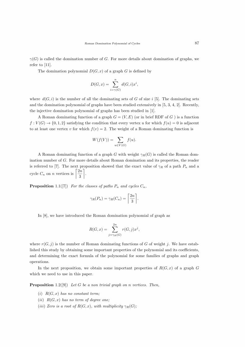
Roman Domination Polynomial of Cycles 87
γ(G) is called the domination number of G. For more details about domination of graphs, we
refer to [11].
The domination polynomial D(G, x) of a graph G is defined by
D(G, x) =
n∑i=γ(G)
d(G, i)xi,
where d(G, i) is the number of all the dominating sets of G of size i [5]. The dominating sets
and the domination polynomial of graphs have been studied extensively in [5, 3, 4, 2]. Recently,
the injective domination polynomial of graphs has been studied in [1].
A Roman dominating function of a graph G = (V,E) (or in brief RDF of G ) is a function
f : V (G)→ {0, 1, 2} satisfying the condition that every vertex u for which f(u) = 0 is adjacent
to at least one vertex v for which f(v) = 2. The weight of a Roman dominating function is
W (f(V )) =∑
u∈V (G)
f(u).
A Roman dominating function of a graph G with weight γR(G) is called the Roman dom-
ination number of G. For more details about Roman domination and its properties, the reader
is referred to [7]. The next proposition showed that the exact value of γR of a path Pn and a
cycle Cn on n vertices is
⌈2n
3
⌉.
Proposition 1.1([7]) For the classes of paths Pn and cycles Cn,
γR(Pn) = γR(Cn) =
⌈2n
3
⌉.
In [8], we have introduced the Roman domination polynomial of graph as
R(G, x) =
2n∑j=γR(G)
r(G, j)xj ,
where r(G, j) is the number of Roman dominating functions of G of weight j. We have estab-
lished this study by obtaining some important properties of the polynomial and its coefficients,
and determining the exact formula of the polynomial for some families of graphs and graph
operations.
In the next proposition, we obtain some important properties of R(G, x) of a graph G
which we need to use in this paper.
Proposition 1.2([9]) Let G be a non trivial graph on n vertices. Then,
(i) R(G, x) has no constant term;
(ii) R(G, x) has no term of degree one;
(iii) Zero is a root of R(G, x), with multiplicity γR(G);
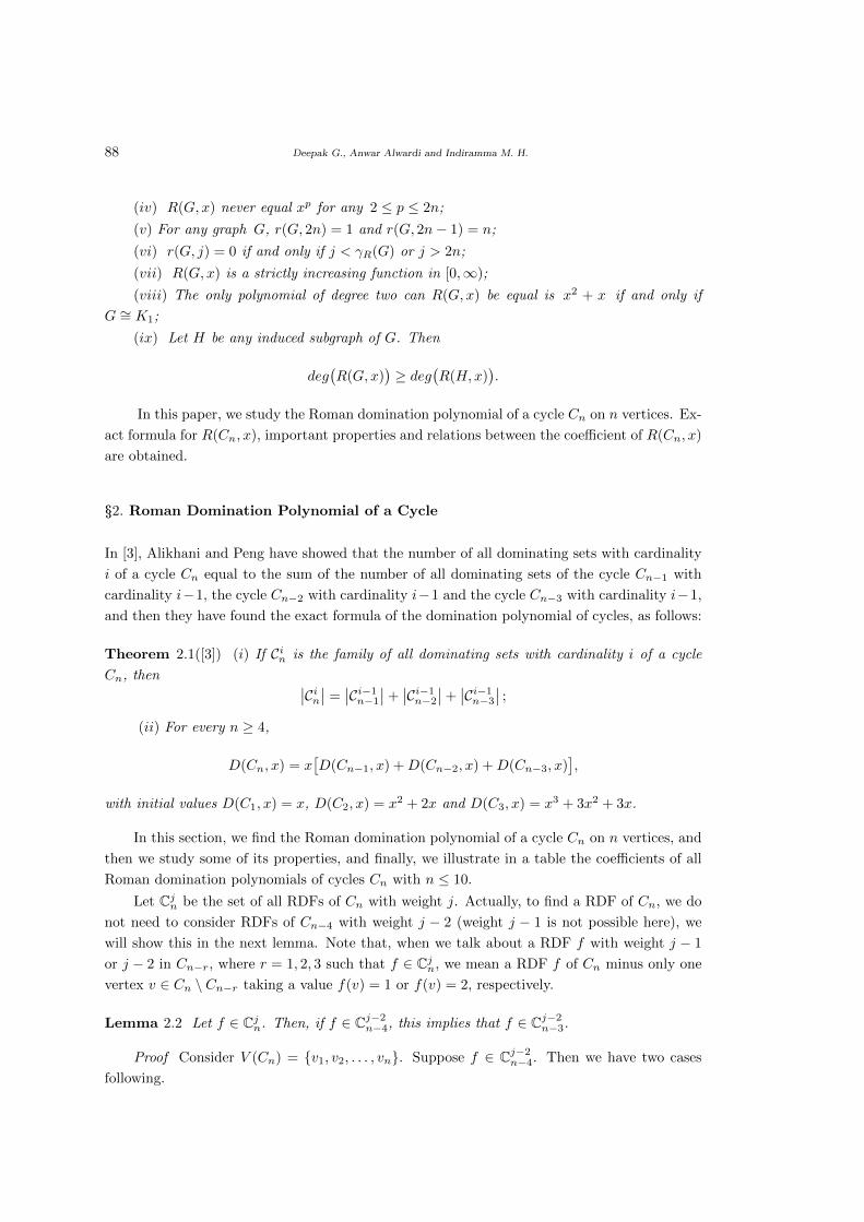
88 Deepak G., Anwar Alwardi and Indiramma M. H.
(iv) R(G, x) never equal xp for any 2 ≤ p ≤ 2n;
(v) For any graph G, r(G, 2n) = 1 and r(G, 2n− 1) = n;
(vi) r(G, j) = 0 if and only if j < γR(G) or j > 2n;
(vii) R(G, x) is a strictly increasing function in [0,∞);
(viii) The only polynomial of degree two can R(G, x) be equal is x2 + x if and only if
G ∼= K1;
(ix) Let H be any induced subgraph of G. Then
deg(R(G, x)
)≥ deg
(R(H,x)
).
In this paper, we study the Roman domination polynomial of a cycle Cn on n vertices. Ex-
act formula for R(Cn, x), important properties and relations between the coefficient of R(Cn, x)
are obtained.
§2. Roman Domination Polynomial of a Cycle
In [3], Alikhani and Peng have showed that the number of all dominating sets with cardinality
i of a cycle Cn equal to the sum of the number of all dominating sets of the cycle Cn−1 with
cardinality i−1, the cycle Cn−2 with cardinality i−1 and the cycle Cn−3 with cardinality i−1,
and then they have found the exact formula of the domination polynomial of cycles, as follows:
Theorem 2.1([3]) (i) If Cin is the family of all dominating sets with cardinality i of a cycle
Cn, then ∣∣Cin∣∣ =∣∣Ci−1n−1
∣∣+∣∣Ci−1n−2
∣∣+∣∣Ci−1n−3
∣∣ ;(ii) For every n ≥ 4,
D(Cn, x) = x[D(Cn−1, x) +D(Cn−2, x) +D(Cn−3, x)
],
with initial values D(C1, x) = x, D(C2, x) = x2 + 2x and D(C3, x) = x3 + 3x2 + 3x.
In this section, we find the Roman domination polynomial of a cycle Cn on n vertices, and
then we study some of its properties, and finally, we illustrate in a table the coefficients of all
Roman domination polynomials of cycles Cn with n ≤ 10.
Let Cjn be the set of all RDFs of Cn with weight j. Actually, to find a RDF of Cn, we do
not need to consider RDFs of Cn−4 with weight j − 2 (weight j − 1 is not possible here), we
will show this in the next lemma. Note that, when we talk about a RDF f with weight j − 1
or j − 2 in Cn−r, where r = 1, 2, 3 such that f ∈ Cjn, we mean a RDF f of Cn minus only one
vertex v ∈ Cn \ Cn−r taking a value f(v) = 1 or f(v) = 2, respectively.
Lemma 2.2 Let f ∈ Cjn. Then, if f ∈ Cj−2n−4, this implies that f ∈ Cj−2
n−3.
Proof Consider V (Cn) = {v1, v2, . . . , vn}. Suppose f ∈ Cj−2n−4. Then we have two cases
following.
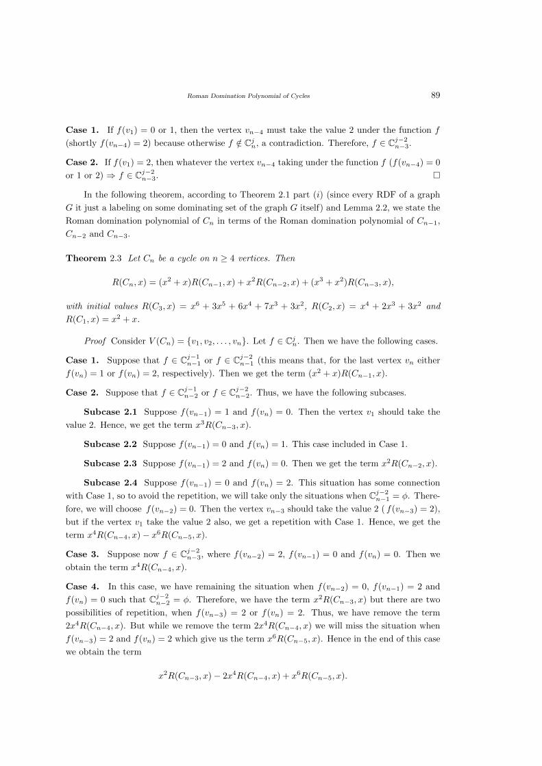
Roman Domination Polynomial of Cycles 89
Case 1. If f(v1) = 0 or 1, then the vertex vn−4 must take the value 2 under the function f
(shortly f(vn−4) = 2) because otherwise f /∈ Cjn, a contradiction. Therefore, f ∈ Cj−2n−3.
Case 2. If f(v1) = 2, then whatever the vertex vn−4 taking under the function f (f(vn−4) = 0
or 1 or 2) ⇒ f ∈ Cj−2n−3. �
In the following theorem, according to Theorem 2.1 part (i) (since every RDF of a graph
G it just a labeling on some dominating set of the graph G itself) and Lemma 2.2, we state the
Roman domination polynomial of Cn in terms of the Roman domination polynomial of Cn−1,
Cn−2 and Cn−3.
Theorem 2.3 Let Cn be a cycle on n ≥ 4 vertices. Then
R(Cn, x) = (x2 + x)R(Cn−1, x) + x2R(Cn−2, x) + (x3 + x2)R(Cn−3, x),
with initial values R(C3, x) = x6 + 3x5 + 6x4 + 7x3 + 3x2, R(C2, x) = x4 + 2x3 + 3x2 and
R(C1, x) = x2 + x.
Proof Consider V (Cn) = {v1, v2, . . . , vn}. Let f ∈ Cjn. Then we have the following cases.
Case 1. Suppose that f ∈ Cj−1n−1 or f ∈ Cj−2
n−1 (this means that, for the last vertex vn either
f(vn) = 1 or f(vn) = 2, respectively). Then we get the term (x2 + x)R(Cn−1, x).
Case 2. Suppose that f ∈ Cj−1n−2 or f ∈ Cj−2
n−2. Thus, we have the following subcases.
Subcase 2.1 Suppose f(vn−1) = 1 and f(vn) = 0. Then the vertex v1 should take the
value 2. Hence, we get the term x3R(Cn−3, x).
Subcase 2.2 Suppose f(vn−1) = 0 and f(vn) = 1. This case included in Case 1.
Subcase 2.3 Suppose f(vn−1) = 2 and f(vn) = 0. Then we get the term x2R(Cn−2, x).
Subcase 2.4 Suppose f(vn−1) = 0 and f(vn) = 2. This situation has some connection
with Case 1, so to avoid the repetition, we will take only the situations when Cj−2n−1 = φ. There-
fore, we will choose f(vn−2) = 0. Then the vertex vn−3 should take the value 2 ( f(vn−3) = 2),
but if the vertex v1 take the value 2 also, we get a repetition with Case 1. Hence, we get the
term x4R(Cn−4, x)− x6R(Cn−5, x).
Case 3. Suppose now f ∈ Cj−2n−3, where f(vn−2) = 2, f(vn−1) = 0 and f(vn) = 0. Then we
obtain the term x4R(Cn−4, x).
Case 4. In this case, we have remaining the situation when f(vn−2) = 0, f(vn−1) = 2 and
f(vn) = 0 such that Cj−2n−2 = φ. Therefore, we have the term x2R(Cn−3, x) but there are two
possibilities of repetition, when f(vn−3) = 2 or f(vn) = 2. Thus, we have remove the term
2x4R(Cn−4, x). But while we remove the term 2x4R(Cn−4, x) we will miss the situation when
f(vn−3) = 2 and f(vn) = 2 which give us the term x6R(Cn−5, x). Hence in the end of this case
we obtain the term
x2R(Cn−3, x)− 2x4R(Cn−4, x) + x6R(Cn−5, x).
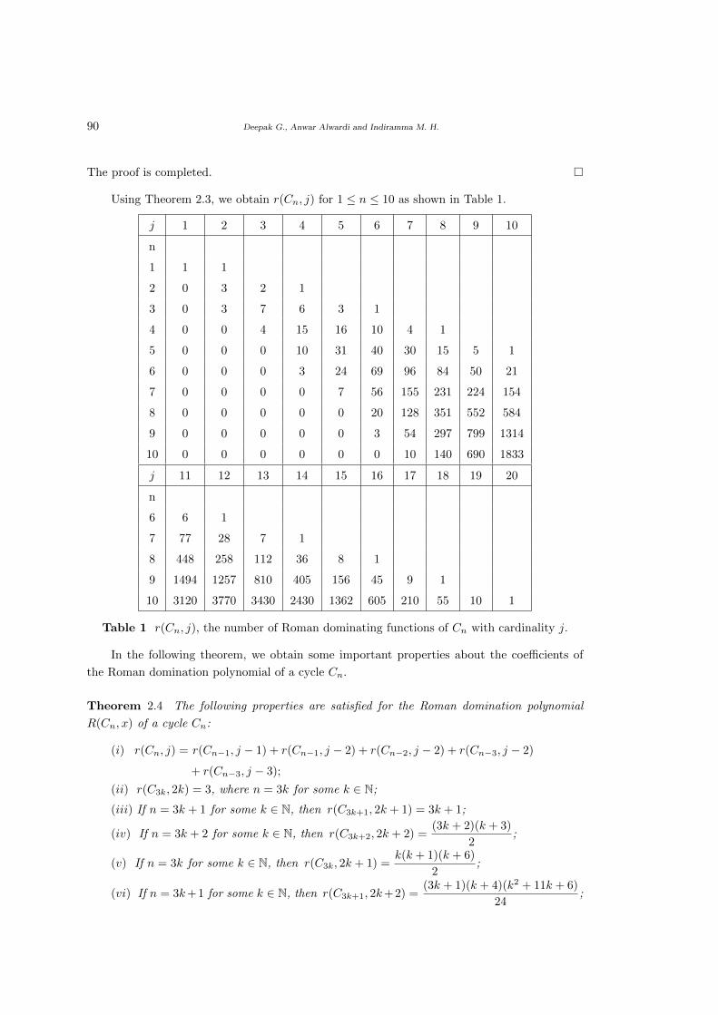
90 Deepak G., Anwar Alwardi and Indiramma M. H.
The proof is completed. �
Using Theorem 2.3, we obtain r(Cn, j) for 1 ≤ n ≤ 10 as shown in Table 1.
j 1 2 3 4 5 6 7 8 9 10
n
1 1 1
2 0 3 2 1
3 0 3 7 6 3 1
4 0 0 4 15 16 10 4 1
5 0 0 0 10 31 40 30 15 5 1
6 0 0 0 3 24 69 96 84 50 21
7 0 0 0 0 7 56 155 231 224 154
8 0 0 0 0 0 20 128 351 552 584
9 0 0 0 0 0 3 54 297 799 1314
10 0 0 0 0 0 0 10 140 690 1833
j 11 12 13 14 15 16 17 18 19 20
n
6 6 1
7 77 28 7 1
8 448 258 112 36 8 1
9 1494 1257 810 405 156 45 9 1
10 3120 3770 3430 2430 1362 605 210 55 10 1
Table 1 r(Cn, j), the number of Roman dominating functions of Cn with cardinality j.
In the following theorem, we obtain some important properties about the coefficients of
the Roman domination polynomial of a cycle Cn.
Theorem 2.4 The following properties are satisfied for the Roman domination polynomial
R(Cn, x) of a cycle Cn:
(i) r(Cn, j) = r(Cn−1, j − 1) + r(Cn−1, j − 2) + r(Cn−2, j − 2) + r(Cn−3, j − 2)
+ r(Cn−3, j − 3);
(ii) r(C3k, 2k) = 3, where n = 3k for some k ∈ N;
(iii) If n = 3k + 1 for some k ∈ N, then r(C3k+1, 2k + 1) = 3k + 1;
(iv) If n = 3k + 2 for some k ∈ N, then r(C3k+2, 2k + 2) =(3k + 2)(k + 3)
2;
(v) If n = 3k for some k ∈ N, then r(C3k, 2k + 1) =k(k + 1)(k + 6)
2;
(vi) If n = 3k+1 for some k ∈ N, then r(C3k+1, 2k+2) =(3k + 1)(k + 4)(k2 + 11k + 6)
24;
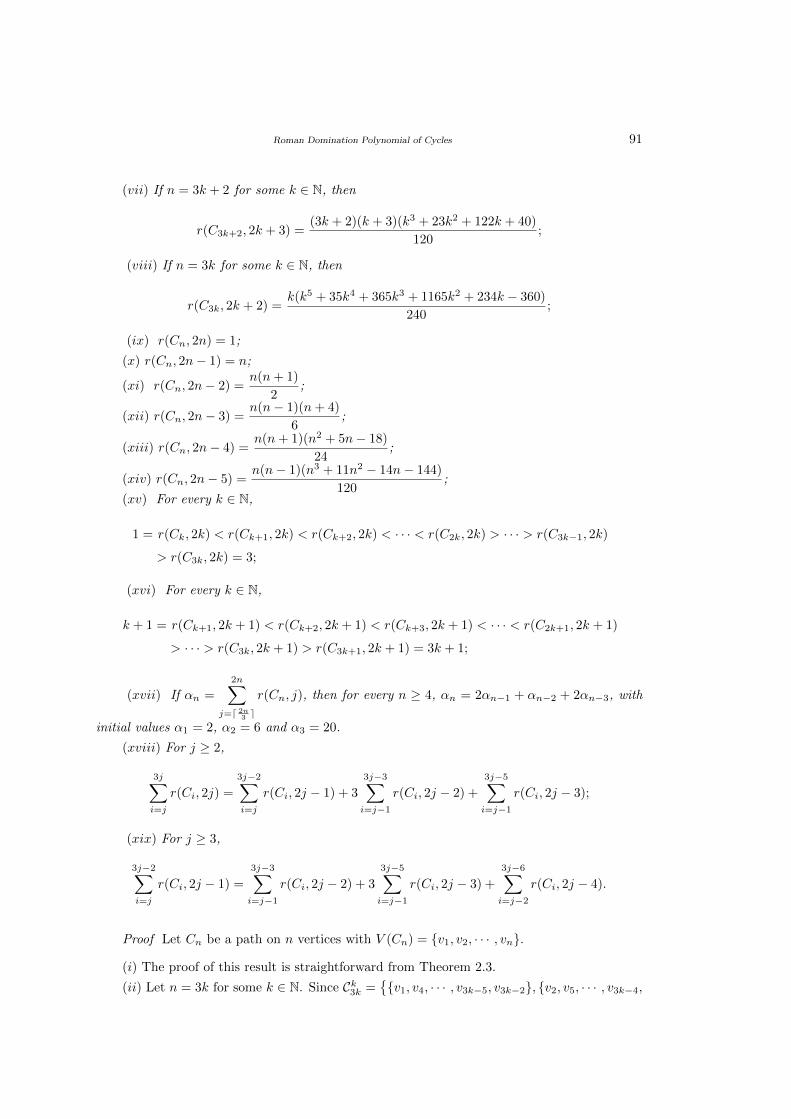
Roman Domination Polynomial of Cycles 91
(vii) If n = 3k + 2 for some k ∈ N, then
r(C3k+2, 2k + 3) =(3k + 2)(k + 3)(k3 + 23k2 + 122k + 40)
120;
(viii) If n = 3k for some k ∈ N, then
r(C3k, 2k + 2) =k(k5 + 35k4 + 365k3 + 1165k2 + 234k − 360)
240;
(ix) r(Cn, 2n) = 1;
(x) r(Cn, 2n− 1) = n;
(xi) r(Cn, 2n− 2) =n(n+ 1)
2;
(xii) r(Cn, 2n− 3) =n(n− 1)(n+ 4)
6;
(xiii) r(Cn, 2n− 4) =n(n+ 1)(n2 + 5n− 18)
24;
(xiv) r(Cn, 2n− 5) =n(n− 1)(n3 + 11n2 − 14n− 144)
120;
(xv) For every k ∈ N,
1 = r(Ck, 2k) < r(Ck+1, 2k) < r(Ck+2, 2k) < · · · < r(C2k, 2k) > · · · > r(C3k−1, 2k)
> r(C3k, 2k) = 3;
(xvi) For every k ∈ N,
k + 1 = r(Ck+1, 2k + 1) < r(Ck+2, 2k + 1) < r(Ck+3, 2k + 1) < · · · < r(C2k+1, 2k + 1)
> · · · > r(C3k, 2k + 1) > r(C3k+1, 2k + 1) = 3k + 1;
(xvii) If αn =
2n∑j=d 2n3 e
r(Cn, j), then for every n ≥ 4, αn = 2αn−1 + αn−2 + 2αn−3, with
initial values α1 = 2, α2 = 6 and α3 = 20.
(xviii) For j ≥ 2,
3j∑i=j
r(Ci, 2j) =
3j−2∑i=j
r(Ci, 2j − 1) + 3
3j−3∑i=j−1
r(Ci, 2j − 2) +
3j−5∑i=j−1
r(Ci, 2j − 3);
(xix) For j ≥ 3,
3j−2∑i=j
r(Ci, 2j − 1) =
3j−3∑i=j−1
r(Ci, 2j − 2) + 3
3j−5∑i=j−1
r(Ci, 2j − 3) +
3j−6∑i=j−2
r(Ci, 2j − 4).
Proof Let Cn be a path on n vertices with V (Cn) = {v1, v2, · · · , vn}.
(i) The proof of this result is straightforward from Theorem 2.3.
(ii) Let n = 3k for some k ∈ N. Since Ck3k ={{v1, v4, · · · , v3k−5, v3k−2}, {v2, v5, · · · , v3k−4,
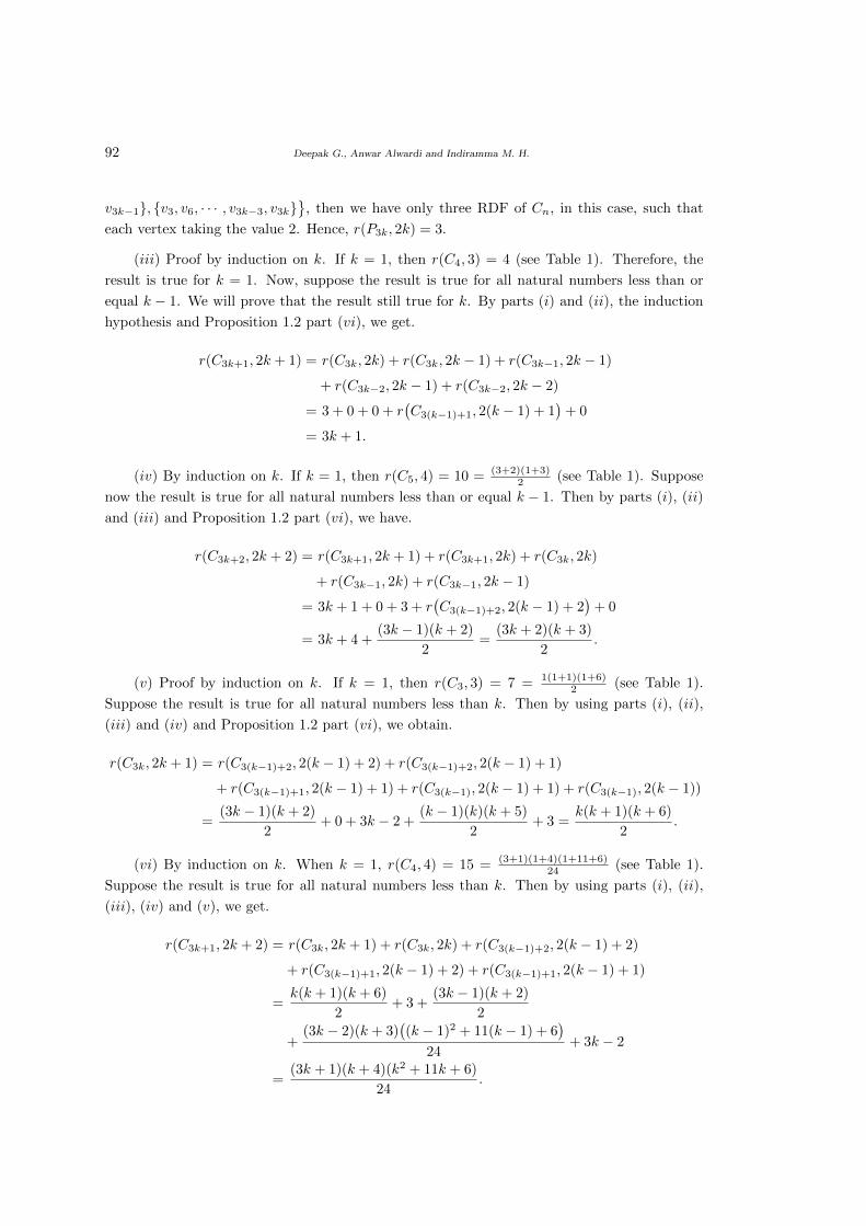
92 Deepak G., Anwar Alwardi and Indiramma M. H.
v3k−1}, {v3, v6, · · · , v3k−3, v3k}}
, then we have only three RDF of Cn, in this case, such that
each vertex taking the value 2. Hence, r(P3k, 2k) = 3.
(iii) Proof by induction on k. If k = 1, then r(C4, 3) = 4 (see Table 1). Therefore, the
result is true for k = 1. Now, suppose the result is true for all natural numbers less than or
equal k − 1. We will prove that the result still true for k. By parts (i) and (ii), the induction
hypothesis and Proposition 1.2 part (vi), we get.
r(C3k+1, 2k + 1) = r(C3k, 2k) + r(C3k, 2k − 1) + r(C3k−1, 2k − 1)
+ r(C3k−2, 2k − 1) + r(C3k−2, 2k − 2)
= 3 + 0 + 0 + r(C3(k−1)+1, 2(k − 1) + 1
)+ 0
= 3k + 1.
(iv) By induction on k. If k = 1, then r(C5, 4) = 10 = (3+2)(1+3)2 (see Table 1). Suppose
now the result is true for all natural numbers less than or equal k − 1. Then by parts (i), (ii)
and (iii) and Proposition 1.2 part (vi), we have.
r(C3k+2, 2k + 2) = r(C3k+1, 2k + 1) + r(C3k+1, 2k) + r(C3k, 2k)
+ r(C3k−1, 2k) + r(C3k−1, 2k − 1)
= 3k + 1 + 0 + 3 + r(C3(k−1)+2, 2(k − 1) + 2
)+ 0
= 3k + 4 +(3k − 1)(k + 2)
2=
(3k + 2)(k + 3)
2.
(v) Proof by induction on k. If k = 1, then r(C3, 3) = 7 = 1(1+1)(1+6)2 (see Table 1).
Suppose the result is true for all natural numbers less than k. Then by using parts (i), (ii),
(iii) and (iv) and Proposition 1.2 part (vi), we obtain.
r(C3k, 2k + 1) = r(C3(k−1)+2, 2(k − 1) + 2) + r(C3(k−1)+2, 2(k − 1) + 1)
+ r(C3(k−1)+1, 2(k − 1) + 1) + r(C3(k−1), 2(k − 1) + 1) + r(C3(k−1), 2(k − 1))
=(3k − 1)(k + 2)
2+ 0 + 3k − 2 +
(k − 1)(k)(k + 5)
2+ 3 =
k(k + 1)(k + 6)
2.
(vi) By induction on k. When k = 1, r(C4, 4) = 15 = (3+1)(1+4)(1+11+6)24 (see Table 1).
Suppose the result is true for all natural numbers less than k. Then by using parts (i), (ii),
(iii), (iv) and (v), we get.
r(C3k+1, 2k + 2) = r(C3k, 2k + 1) + r(C3k, 2k) + r(C3(k−1)+2, 2(k − 1) + 2)
+ r(C3(k−1)+1, 2(k − 1) + 2) + r(C3(k−1)+1, 2(k − 1) + 1)
=k(k + 1)(k + 6)
2+ 3 +
(3k − 1)(k + 2)
2
+(3k − 2)(k + 3)
((k − 1)2 + 11(k − 1) + 6
)24
+ 3k − 2
=(3k + 1)(k + 4)(k2 + 11k + 6)
24.
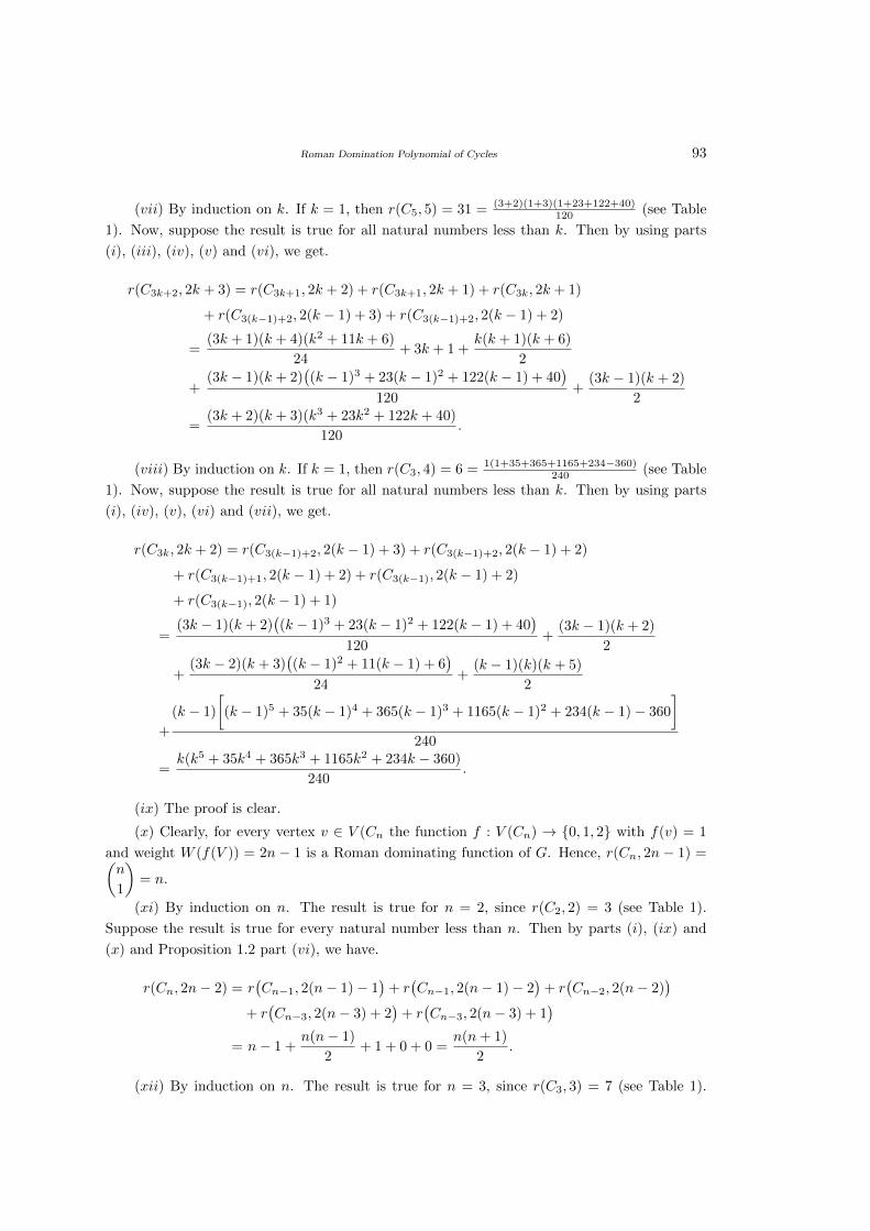
Roman Domination Polynomial of Cycles 93
(vii) By induction on k. If k = 1, then r(C5, 5) = 31 = (3+2)(1+3)(1+23+122+40)120 (see Table
1). Now, suppose the result is true for all natural numbers less than k. Then by using parts
(i), (iii), (iv), (v) and (vi), we get.
r(C3k+2, 2k + 3) = r(C3k+1, 2k + 2) + r(C3k+1, 2k + 1) + r(C3k, 2k + 1)
+ r(C3(k−1)+2, 2(k − 1) + 3) + r(C3(k−1)+2, 2(k − 1) + 2)
=(3k + 1)(k + 4)(k2 + 11k + 6)
24+ 3k + 1 +
k(k + 1)(k + 6)
2
+(3k − 1)(k + 2)
((k − 1)3 + 23(k − 1)2 + 122(k − 1) + 40
)120
+(3k − 1)(k + 2)
2
=(3k + 2)(k + 3)(k3 + 23k2 + 122k + 40)
120.
(viii) By induction on k. If k = 1, then r(C3, 4) = 6 = 1(1+35+365+1165+234−360)240 (see Table
1). Now, suppose the result is true for all natural numbers less than k. Then by using parts
(i), (iv), (v), (vi) and (vii), we get.
r(C3k, 2k + 2) = r(C3(k−1)+2, 2(k − 1) + 3) + r(C3(k−1)+2, 2(k − 1) + 2)
+ r(C3(k−1)+1, 2(k − 1) + 2) + r(C3(k−1), 2(k − 1) + 2)
+ r(C3(k−1), 2(k − 1) + 1)
=(3k − 1)(k + 2)
((k − 1)3 + 23(k − 1)2 + 122(k − 1) + 40
)120
+(3k − 1)(k + 2)
2
+(3k − 2)(k + 3)
((k − 1)2 + 11(k − 1) + 6
)24
+(k − 1)(k)(k + 5)
2
+
(k − 1)
[(k − 1)5 + 35(k − 1)4 + 365(k − 1)3 + 1165(k − 1)2 + 234(k − 1)− 360
]240
=k(k5 + 35k4 + 365k3 + 1165k2 + 234k − 360)
240.
(ix) The proof is clear.
(x) Clearly, for every vertex v ∈ V (Cn the function f : V (Cn) → {0, 1, 2} with f(v) = 1
and weight W (f(V )) = 2n − 1 is a Roman dominating function of G. Hence, r(Cn, 2n − 1) =(n
1
)= n.
(xi) By induction on n. The result is true for n = 2, since r(C2, 2) = 3 (see Table 1).
Suppose the result is true for every natural number less than n. Then by parts (i), (ix) and
(x) and Proposition 1.2 part (vi), we have.
r(Cn, 2n− 2) = r(Cn−1, 2(n− 1)− 1
)+ r(Cn−1, 2(n− 1)− 2
)+ r(Cn−2, 2(n− 2)
)+ r(Cn−3, 2(n− 3) + 2
)+ r(Cn−3, 2(n− 3) + 1
)= n− 1 +
n(n− 1)
2+ 1 + 0 + 0 =
n(n+ 1)
2.
(xii) By induction on n. The result is true for n = 3, since r(C3, 3) = 7 (see Table 1).
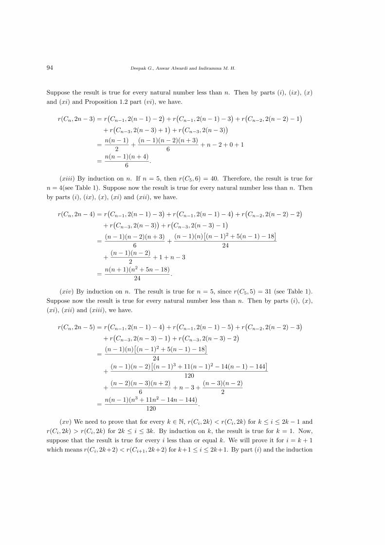
94 Deepak G., Anwar Alwardi and Indiramma M. H.
Suppose the result is true for every natural number less than n. Then by parts (i), (ix), (x)
and (xi) and Proposition 1.2 part (vi), we have.
r(Cn, 2n− 3) = r(Cn−1, 2(n− 1)− 2
)+ r(Cn−1, 2(n− 1)− 3
)+ r(Cn−2, 2(n− 2)− 1
)+ r(Cn−3, 2(n− 3) + 1
)+ r(Cn−3, 2(n− 3)
)=n(n− 1)
2+
(n− 1)(n− 2)(n+ 3)
6+ n− 2 + 0 + 1
=n(n− 1)(n+ 4)
6.
(xiii) By induction on n. If n = 5, then r(C5, 6) = 40. Therefore, the result is true for
n = 4(see Table 1). Suppose now the result is true for every natural number less than n. Then
by parts (i), (ix), (x), (xi) and (xii), we have.
r(Cn, 2n− 4) = r(Cn−1, 2(n− 1)− 3
)+ r(Cn−1, 2(n− 1)− 4
)+ r(Cn−2, 2(n− 2)− 2
)+ r(Cn−3, 2(n− 3)
)+ r(Cn−3, 2(n− 3)− 1
)=
(n− 1)(n− 2)(n+ 3)
6+
(n− 1)(n)[(n− 1)2 + 5(n− 1)− 18
]24
+(n− 1)(n− 2)
2+ 1 + n− 3
=n(n+ 1)(n2 + 5n− 18)
24.
(xiv) By induction on n. The result is true for n = 5, since r(C5, 5) = 31 (see Table 1).
Suppose now the result is true for every natural number less than n. Then by parts (i), (x),
(xi), (xii) and (xiii), we have.
r(Cn, 2n− 5) = r(Cn−1, 2(n− 1)− 4
)+ r(Cn−1, 2(n− 1)− 5
)+ r(Cn−2, 2(n− 2)− 3
)+ r(Cn−3, 2(n− 3)− 1
)+ r(Cn−3, 2(n− 3)− 2
)=
(n− 1)(n)[(n− 1)2 + 5(n− 1)− 18
]24
+(n− 1)(n− 2)
[(n− 1)3 + 11(n− 1)2 − 14(n− 1)− 144
]120
+(n− 2)(n− 3)(n+ 2)
6+ n− 3 +
(n− 3)(n− 2)
2
=n(n− 1)(n3 + 11n2 − 14n− 144)
120.
(xv) We need to prove that for every k ∈ N, r(Ci, 2k) < r(Ci, 2k) for k ≤ i ≤ 2k − 1 and
r(Ci, 2k) > r(Ci, 2k) for 2k ≤ i ≤ 3k. By induction on k, the result is true for k = 1. Now,
suppose that the result is true for every i less than or equal k. We will prove it for i = k + 1
which means r(Ci, 2k+2) < r(Ci+1, 2k+2) for k+1 ≤ i ≤ 2k+1. By part (i) and the induction
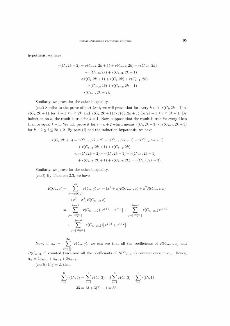
Roman Domination Polynomial of Cycles 95
hypothesis, we have
r(Ci, 2k + 2) = r(Ci−1, 2k + 1) + r(Ci−1, 2k) + r(Ci−2, 2k)
+ r(Ci−3, 2k) + r(Ci−3, 2k − 1)
<r(Ci, 2k + 1) + r(Ci, 2k) + r(Ci−1, 2k)
+ r(Ci−2, 2k) + r(Ci−2, 2k − 1)
=r(Ci+1, 2k + 2).
Similarly, we prove for the other inequality.
(xvi) Similar to the prove of part (xv), we will prove that for every k ∈ N, r(Ci, 2k+ 1) <
r(Ci, 2k + 1) for k + 1 ≤ i ≤ 2k and r(Ci, 2k + 1) > r(Ci, 2k + 1) for 2k + 1 ≤ i ≤ 3k + 1. By
induction on k, the result is true for k = 1. Now, suppose that the result is true for every i less
than or equal k+ 1. We will prove it for i = k+ 2 which means r(Ci, 2k+ 3) < r(Ci+1, 2k+ 3)
for k + 2 ≤ i ≤ 2k + 2. By part (i) and the induction hypothesis, we have
r(Ci, 2k + 3) = r(Ci−1, 2k + 2) + r(Ci−1, 2k + 1) + r(Ci−2, 2k + 1)
+ r(Ci−3, 2k + 1) + r(Ci−3, 2k)
< r(Ci, 2k + 2) + r(Ci, 2k + 1) + r(Ci−1, 2k + 1)
+ r(Ci−2, 2k + 1) + r(Ci−2, 2k) = r(Ci+1, 2k + 3).
Similarly, we prove for the other inequality.
(xvii) By Theorem 2.3, we have
R(Cn, x) =
2n∑j=γR(Cn)
r(Cn, j)xj = (x2 + x)R(Cn−1, x) + x2R(Cn−2, x)
+ (x3 + x2)R(Cn−3, x)
=
2n−2∑j=d 2n−2
3 e
r(Cn−1, j)[xj+2 + xj+1
]+
2n−4∑j=d 2n−4
3 e
r(Cn−2, j)xj+2
+
2n−6∑j=d 2n−6
3 e
r(Cn−3, j)[xj+3 + xj+2
].
Now, if αn =
2n∑j=d 2n3 e
r(Cn, j), we can see that all the coefficients of R(Cn−1, x) and
R(Cn−3, x) counted twice and all the coefficients of R(Cn−2, x) counted once in αn. Hence,
αn = 2αn−1 + αn−2 + 2αn−3.
(xviii) If j = 2, then
6∑i=2
r(Ci, 4) =
4∑i=2
r(Ci, 3) + 3
3∑i=1
r(Ci, 2) +
1∑i=1
r(Ci, 1)
35 = 13 + 3(7) + 1 = 35.
96 Deepak G., Anwar Alwardi and Indiramma M. H.
By part (i), we have
3j∑i=j
r(Ci, 2j) =
3j∑i=j
r(Ci−1, 2j − 1) +
3j∑i=j
r(Ci−1, 2j − 2) +
3j∑i=j
r(Ci−2, 2j − 2)
+
3j∑i=j
r(Ci−3, 2j − 2) +
3j∑i=j
r(Ci−3, 2j − 3).
Now, by Proposition 1.2 part (vi), we have
3j∑i=j
r(Ci−1, 2j − 1) =
3j∑i=j−1
r(Ci, 2j − 1) =
3j−2∑i=j
r(Ci, 2j − 1),
3j∑i=j
r(Ci−1, 2j − 2) =
3j∑i=j−1
r(Ci, 2j − 2) =
3j−3∑i=j−1
r(Ci, 2j − 2),
3j∑i=j
r(Ci−2, 2j − 2) =
3j∑i=j−2
r(Ci, 2j − 2) =
3j−3∑i=j−1
r(Ci, 2j − 2),
3j∑i=j
r(Ci−3, 2j − 2) =
3j∑i=j−3
r(Ci, 2j − 2) =
3j−3∑i=j−1
r(Ci, 2j − 2)
and3j∑i=j
r(Ci−3, 2j − 3) =
3j∑i=j−3
r(Ci, 2j − 3) =
3j−5∑i=j−1
r(Ci, 2j − 3).
(xix) The proof is similar to the proof of part (xviii). �
References
[1] Akram Alqesmah, Anwar Alwardi and R. Rangarajan, On the Injective domination Poly-
nomial of graphs, Palestine journal of Mathematics, 7 (1) (2018) 234–242.
[2] S. Alikhani, Y. H. Peng, Dominating sets and domination polynomial of certain graphs,
II, Opuscula Mathematica, 30 (1) (2010) 37–51.
[3] S. Alikhani, Y.H. Peng, Dominating sets and domination polynomial of cycles, Global
Journal of Pure and Applied Mathematics, 4 (2) (2008) 151–162.
[4] S. Alikhani, Y.H. Peng, Dominating sets and domination polynomial of paths, International
Journal of Mathematics and Mathematical Sciences, Article ID 542040, doi:10.1155/2009/
542040, (2009).
[5] S. Alikhani, Y.H. Peng, Introduction to domination polynomial of a graph, Ars Combin.,
114 (2014) 257–266.
[6] J. A. Bondy, U. S. R. Murty, Graph Theory with Applications, The Macmillan Press Ltd.,
London, Basingstoke, 1976.
[7] Ernie J. Cockayne, Paul A. Dreyer Jr., Sandra M. Hedetniemi and Stephen T. Hedetniemi,
Roman domination in graphs, Discrete Mathematics, 278 (2004) 11–22.
Roman Domination Polynomial of Cycles 97
[8] Deepak G., Indiramma M. H., Anwar Alwardi and Indiramma M. H., Roman domination
polynomial on paths, Palestine Journal of Mathematics (will Appear).
[9] Deepak G., Indiramma M. H., N. D. Soner and Anwar Alwardi, On the Roman distri-
bution polynomial of graphs, Bulletin of the International Mathematical Virtual Institute,
11(2)(2021),355-365.
[10] F. Harary, Graph Theory, Addison-Wesley, Reading Mass (1969).
[11] T. W. Haynes, S. T. Hedetniemi and P. J. Slater, Fundamentals of Domination in Graphs,
Marcel Dekker, Inc., New York (1998).
[12] W. X. Hong, L. H. You, On the eigenvalues of firefly graphs, Transactions on Combina-
torics, 3 (3) (2014) 1–9.
[13] I. Stewart, Defend the Roman empire, Sci. Amer., 281 (6) (1999) 136–139.
International J.Math. Combin. Vol.3(2021), 98-104
Application of
Abstract Algebra to Musical Notes and Indian Music
Ram Milan Singh
(Department of mathematics, Government Post Graduate College, Tikamgarh, India)
Abstract: This paper critically analysis the behavior and the relationship that exist be-
tween musical notes and abstract algebra. The musical notes form additive Abelian group
modulo 12. Finally, the work come up with some propositions due to the musical notes
behavior and their proofs, one of which was name Dido’s Theorem.
Key Words: Abstract algebra, Abelian group modulo 12, Abelian group modulo 7, musical
notes, Indian sargam, Dido’s Theorem, transposition, inversion, Smarandache multigroup.
AMS(2010): 30K20.
§1. Introduction
In mathematics and group theory, abstract algebra, studies the algebraic structures known as
groups. The concept of a group is central to abstract algebra. Other well-known algebraic
structures, such as rings, fields, and vectors space can all be seen as groups endowed with ad-
ditional operations and axioms. Various physical systems, such as crystals and the hydrogen
atom, can be modeled by symmetry groups. Thus, abstract algebra has many important appli-
cations in physics, chemistry, and materials science. Abstract algebra is also central to public
key cryptography. The modern concept of abstract group developed out of several fields of
mathematics (Wussing, 2007). The idea of group theory although developed from the concept
of abstract algebra, yet can be applied in many other areas of mathematical areas and other
field in sciences and as well as in music. Music theory is a big field within mathematics and lots
of different people have taken it in different directions. Music is that one of the fine arts which
is concerned with the combination of sounds with a view to beauty of form and the expression
of thought or feeling. Music itself is not complete without musical notes. And the musical
notes and Indian music are: C,C#,D,D#,E,F,F#,G,G#,A,A#,B. Now in India, Indian
seven sargam are: Sa. Re, Ga, Ma, Pa, Dha, Ni. For years, many people find it difficult to
comprehend some concept in group theory satisfactorily, but with the behavior of these musical
notes, group theory can be studied. “All is number” (only musical notes) is the motto of the
Pythagorean School. This school was founded by the Greek mathematician and philosopher
Pythagoras (ca. 580-500 B.C.). The members of the school pursued the study of mathematics,
philosophy, astronomy and music.
1Received June 17, 2021, Accepted September 5, 2021.
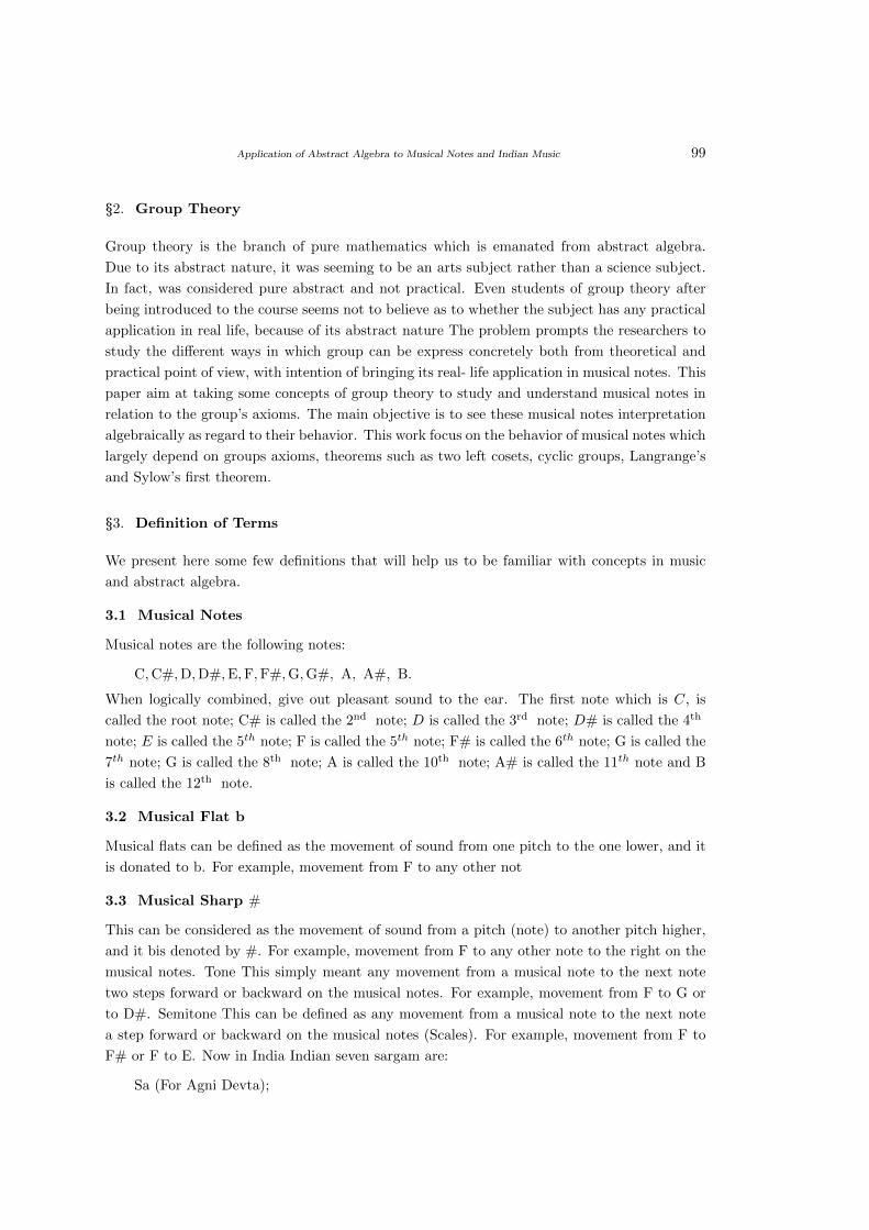
Application of Abstract Algebra to Musical Notes and Indian Music 99
§2. Group Theory
Group theory is the branch of pure mathematics which is emanated from abstract algebra.
Due to its abstract nature, it was seeming to be an arts subject rather than a science subject.
In fact, was considered pure abstract and not practical. Even students of group theory after
being introduced to the course seems not to believe as to whether the subject has any practical
application in real life, because of its abstract nature The problem prompts the researchers to
study the different ways in which group can be express concretely both from theoretical and
practical point of view, with intention of bringing its real- life application in musical notes. This
paper aim at taking some concepts of group theory to study and understand musical notes in
relation to the group’s axioms. The main objective is to see these musical notes interpretation
algebraically as regard to their behavior. This work focus on the behavior of musical notes which
largely depend on groups axioms, theorems such as two left cosets, cyclic groups, Langrange’s
and Sylow’s first theorem.
§3. Definition of Terms
We present here some few definitions that will help us to be familiar with concepts in music
and abstract algebra.
3.1 Musical Notes
Musical notes are the following notes:
C,C#,D,D#,E,F,F#,G,G#, A, A#, B.
When logically combined, give out pleasant sound to the ear. The first note which is C, is
called the root note; C# is called the 2nd note; D is called the 3rd note; D# is called the 4th
note; E is called the 5th note; F is called the 5th note; F# is called the 6th note; G is called the
7th note; G is called the 8th note; A is called the 10th note; A# is called the 11th note and B
is called the 12th note.
3.2 Musical Flat b
Musical flats can be defined as the movement of sound from one pitch to the one lower, and it
is donated to b. For example, movement from F to any other not
3.3 Musical Sharp #
This can be considered as the movement of sound from a pitch (note) to another pitch higher,
and it bis denoted by #. For example, movement from F to any other note to the right on the
musical notes. Tone This simply meant any movement from a musical note to the next note
two steps forward or backward on the musical notes. For example, movement from F to G or
to D#. Semitone This can be defined as any movement from a musical note to the next note
a step forward or backward on the musical notes (Scales). For example, movement from F to
F# or F to E. Now in India Indian seven sargam are:
Sa (For Agni Devta);
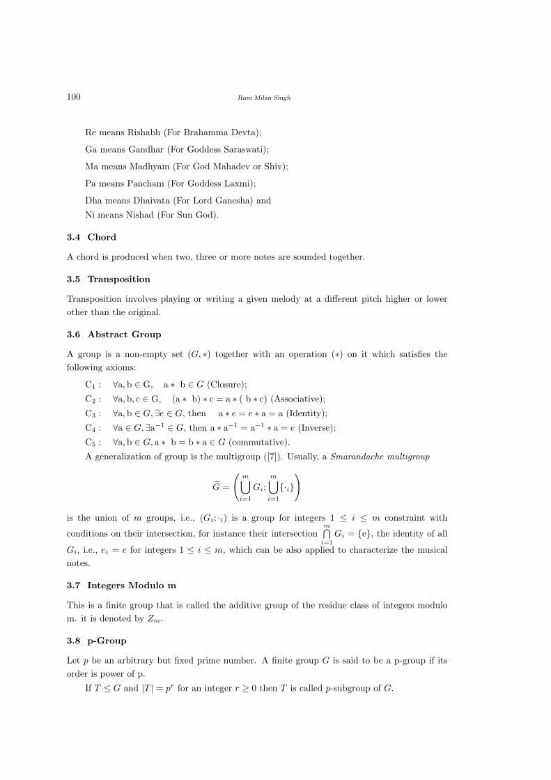
100 Ram Milan Singh
Re means Rishabh (For Brahamma Devta);
Ga means Gandhar (For Goddess Saraswati);
Ma means Madhyam (For God Mahadev or Shiv);
Pa means Pancham (For Goddess Laxmi);
Dha means Dhaivata (For Lord Ganesha) and
Ni means Nishad (For Sun God).
3.4 Chord
A chord is produced when two, three or more notes are sounded together.
3.5 Transposition
Transposition involves playing or writing a given melody at a different pitch higher or lower
other than the original.
3.6 Abstract Group
A group is a non-empty set (G, ∗) together with an operation (∗) on it which satisfies the
following axioms:
C1 : ∀a,b ∈ G, a ∗ b ∈ G (Closure);
C2 : ∀a,b, c ∈ G, (a ∗ b) ∗ c = a ∗ ( b ∗ c) (Associative);
C3 : ∀a,b ∈ G,∃e ∈ G, then a ∗ e = e ∗ a = a (Identity);
C4 : ∀a ∈ G,∃a−1 ∈ G, then a ∗ a−1 = a−1 ∗ a = e (Inverse);
C5 : ∀a,b ∈ G, a ∗ b = b ∗ a ∈ G (commutative).
A generalization of group is the multigroup ([7]). Usually, a Smarandache multigroup
G =
(m⋃i=1
Gi;
m⋃i=1
{·i}
)
is the union of m groups, i.e., (Gi; ·i) is a group for integers 1 ≤ i ≤ m constraint with
conditions on their intersection, for instance their intersectionm⋂i=1
Gi = {e}, the identity of all
Gi, i.e., ei = e for integers 1 ≤ i ≤ m, which can be also applied to characterize the musical
notes.
3.7 Integers Modulo m
This is a finite group that is called the additive group of the residue class of integers modulo
m. it is denoted by Zm.
3.8 p-Group
Let p be an arbitrary but fixed prime number. A finite group G is said to be a p-group if its
order is power of p.
If T ≤ G and |T | = pr for an integer r ≥ 0 then T is called p-subgroup of G.
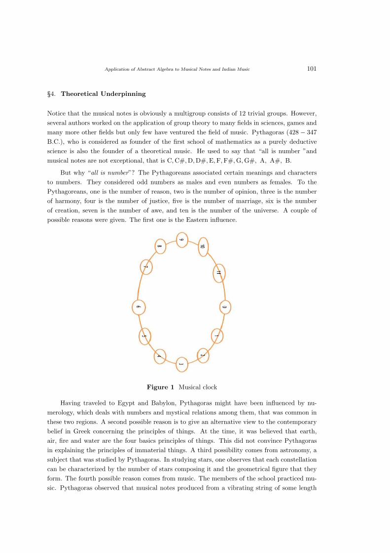
Application of Abstract Algebra to Musical Notes and Indian Music 101
§4. Theoretical Underpinning
Notice that the musical notes is obviously a multigroup consists of 12 trivial groups. However,
several authors worked on the application of group theory to many fields in sciences, games and
many more other fields but only few have ventured the field of music. Pythagoras (428 − 347
B.C.), who is considered as founder of the first school of mathematics as a purely deductive
science is also the founder of a theoretical music. He used to say that “all is number ”and
musical notes are not exceptional, that is C,C#,D,D#,E,F,F#,G,G#, A, A#, B.
But why “all is number”? The Pythagoreans associated certain meanings and characters
to numbers. They considered odd numbers as males and even numbers as females. To the
Pythagoreans, one is the number of reason, two is the number of opinion, three is the number
of harmony, four is the number of justice, five is the number of marriage, six is the number
of creation, seven is the number of awe, and ten is the number of the universe. A couple of
possible reasons were given. The first one is the Eastern influence.
Figure 1 Musical clock
Having traveled to Egypt and Babylon, Pythagoras might have been influenced by nu-
merology, which deals with numbers and mystical relations among them, that was common in
these two regions. A second possible reason is to give an alternative view to the contemporary
belief in Greek concerning the principles of things. At the time, it was believed that earth,
air, fire and water are the four basics principles of things. This did not convince Pythagoras
in explaining the principles of immaterial things. A third possibility comes from astronomy, a
subject that was studied by Pythagoras. In studying stars, one observes that each constellation
can be characterized by the number of stars composing it and the geometrical figure that they
form. The fourth possible reason comes from music. The members of the school practiced mu-
sic. Pythagoras observed that musical notes produced from a vibrating string of some length
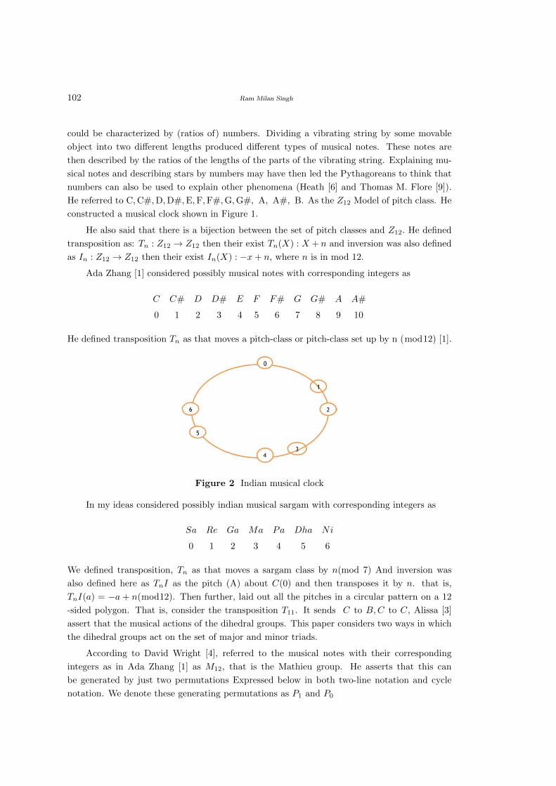
102 Ram Milan Singh
could be characterized by (ratios of) numbers. Dividing a vibrating string by some movable
object into two different lengths produced different types of musical notes. These notes are
then described by the ratios of the lengths of the parts of the vibrating string. Explaining mu-
sical notes and describing stars by numbers may have then led the Pythagoreans to think that
numbers can also be used to explain other phenomena (Heath [6] and Thomas M. Flore [9]).
He referred to C,C#,D,D#,E,F,F#,G,G#, A, A#, B. As the Z12 Model of pitch class. He
constructed a musical clock shown in Figure 1.
He also said that there is a bijection between the set of pitch classes and Z12. He defined
transposition as: Tn : Z12 → Z12 then their exist Tn(X) : X + n and inversion was also defined
as In : Z12 → Z12 then their exist In(X) : −x+ n, where n is in mod 12.
Ada Zhang [1] considered possibly musical notes with corresponding integers as
C C# D D# E F F# G G# A A#
0 1 2 3 4 5 6 7 8 9 10
He defined transposition Tn as that moves a pitch-class or pitch-class set up by n (mod12) [1].
Figure 2 Indian musical clock
In my ideas considered possibly indian musical sargam with corresponding integers as
Sa Re Ga Ma Pa Dha Ni
0 1 2 3 4 5 6
We defined transposition, Tn as that moves a sargam class by n(mod 7) And inversion was
also defined here as TnI as the pitch (A) about C(0) and then transposes it by n. that is,
TnI(a) = −a + n(mod12). Then further, laid out all the pitches in a circular pattern on a 12
-sided polygon. That is, consider the transposition T11. It sends C to B,C to C, Alissa [3]
assert that the musical actions of the dihedral groups. This paper considers two ways in which
the dihedral groups act on the set of major and minor triads.
According to David Wright [4], referred to the musical notes with their corresponding
integers as in Ada Zhang [1] as M12, that is the Mathieu group. He asserts that this can
be generated by just two permutations Expressed below in both two-line notation and cycle
notation. We denote these generating permutations as P1 and P0
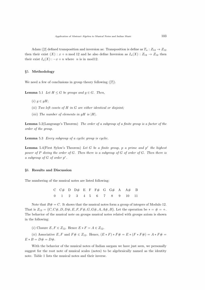
Application of Abstract Algebra to Musical Notes and Indian Music 103
Adam ([2] defined transposition and inversion as: Transposition is define as Tn : Z12 → Z12
then their exist (X) : x + n mod 12 and he also define Inversion as In(X) : Z12 → Z12 then
their exist In(X) : −x+ n where n is in mod12.
§5. Methodology
We need a few of conclusions in group theory following ([7]).
Lemma 5.1 Let H ≤ G be groups and g ∈ G. Then,
(i) g ∈ gH;
(ii) Two left cosets of H in G are either identical or disjoint;
(iii) The number of elements in gH is |H|.
Lemma 5.2(Langrange’s Theorem) The order of a subgroup of a finite group is a factor of the
order of the group.
Lemma 5.3 Every subgroup of a cyclic group is cyclic.
Lemma 5.4(First Sylow’s Theorem) Let G be a finite group, p a prime and pr the highest
power of P diving the order of G. Then there is a subgroup of G of order of G. Then there is
a subgroup of G of order pr.
§6. Results and Discussion
The numbering of the musical notes are listed following:
C C# D D# E F F# G G# A A# B
0 1 2 3 4 5 6 7 8 9 10 11
Note that B# = C. It shows that the musical notes form a group of integers of Modulo 12.
That is Z12 = {C,C#, D,D#, E, F, F#, G,G#, A,A#, B}. Let the operation be ∗ = # = +.
The behavior of the musical note on groups musical notes related with groups axiom is shown
in the following:
(i) Closure E,F ∈ Z12. Hence E ∗ F = A ∈ Z12.
(ii) Associative E,F and F# ∈ Z12. Hence, (E ∗ F ) ∗ F# = E ∗ (F ∗ F#) = A ∗ F# =
E ∗B = D# = D#.
With the behavior of the musical notes of Indian sargam we have just seen, we personally
suggest for the root note of musical scales (notes) to be algebraically named as the identity
note. Table 1 lists the musical notes and their inverse.
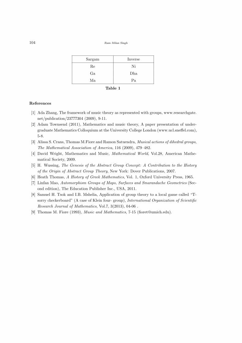
104 Ram Milan Singh
Sargam Inverse
Re Ni
Ga Dha
Ma Pa
Table 1
References
[1] Ada Zhang, The framework of music theory as represented with groups, www.researchgate.
net/publication/23777304 (2009), 9-11.
[2] Adam Townsend (2011), Mathematics and music theory, A paper presentation of under-
graduate Mathematics Colloquium at the University College London (www.ucl.sneffel.com),
5-8.
[3] Alissa S. Crans, Thomas M.Fiore and Ramon Satuendra, Musical actions of dihedral groups,
The Mathematical Association of America, 116 (2009), 479–482.
[4] David Wright, Mathematics and Music, Mathematical World, Vol.28, American Mathe-
matical Society, 2009.
[5] H. Wussing, The Genesis of the Abstract Group Concept: A Contribution to the History
of the Origin of Abstract Group Theory, New York: Dover Publications, 2007.
[6] Heath Thomas, A History of Greek Mathematics, Vol. 1, Oxford University Press, 1965.
[7] Linfan Mao, Automorphism Groups of Maps, Surfaces and Smarandache Geometries (Sec-
ond edition), The Education Publisher Inc., USA, 2011.
[8] Samuel H. Tsok and I.B. Mshelia, Application of group theory to a local game called “T-
sorry checkerboard” (A case of Klein four- group), International Organization of Scientific
Research Journal of Mathematics, Vol.7, 3(2013), 04-06 .
[9] Thomas M. Fiore (1993), Music and Mathematics, 7-15 ([email protected]).
Famous Words
What we know is very slight, what we don’t know is immense. Man follows only phantoms.
By Pierre-Simon Laplace, a French mathematician and also a physicist
Author Information
Submission: Papers only in electronic form are considered for possible publication. Papers
prepared in formats, viz., .tex, .dvi, .pdf, or.ps may be submitted electronically to one member
of the Editorial Board for consideration in the International Journal of Mathematical
Combinatorics (ISSN 1937-1055). An effort is made to publish a paper duly recommended
by a referee within a period of 3 − 4 months. Articles received are immediately put the ref-
erees/members of the Editorial Board for their opinion who generally pass on the same in six
week’s time or less. In case of clear recommendation for publication, the paper is accommo-
dated in an issue to appear next. Each submitted paper is not returned, hence we advise the
authors to keep a copy of their submitted papers for further processing.
Abstract: Authors are requested to provide an abstract of not more than 250 words, lat-
est Mathematics Subject Classification of the American Mathematical Society, Keywords and
phrases. Statements of Lemmas, Propositions and Theorems should be set in italics and ref-
erences should be arranged in alphabetical order by the surname of the first author in the
following style:
Books
[4]Linfan Mao, Combinatorial Geometry with Applications to Field Theory, InfoQuest Press,
2009.
[12]W.S.Massey, Algebraic topology: an introduction, Springer-Verlag, New York 1977.
Research papers
[6]Linfan Mao, Mathematics on non-mathematics - A combinatorial contribution, International
J.Math. Combin., Vol.3(2014), 1-34.
[9]Kavita Srivastava, On singular H-closed extensions, Proc. Amer. Math. Soc. (to appear).
Figures: Figures should be drawn by TEXCAD in text directly, or as EPS file. In addition,
all figures and tables should be numbered and the appropriate space reserved in the text, with
the insertion point clearly indicated.
Copyright: It is assumed that the submitted manuscript has not been published and will
not be simultaneously submitted or published elsewhere. By submitting a manuscript, the
authors agree that the copyright for their articles is transferred to the publisher, if and when,
the paper is accepted for publication. The publisher cannot take the responsibility of any loss
of manuscript. Therefore, authors are requested to maintain a copy at their end.
Proofs: One set of galley proofs of a paper will be sent to the author submitting the paper,
unless requested otherwise, without the original manuscript, for corrections after the paper is
accepted for publication on the basis of the recommendation of referees. Corrections should be
restricted to typesetting errors. Authors are advised to check their proofs very carefully before
return.
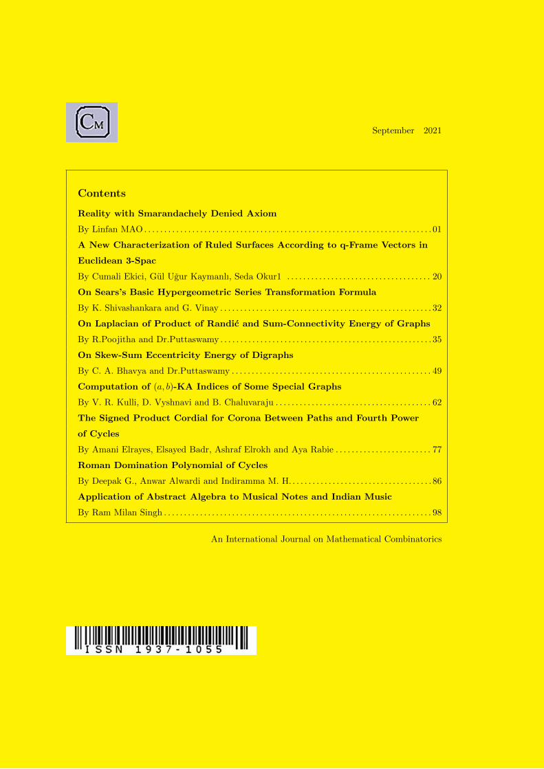
September 2021
Contents
Reality with Smarandachely Denied Axiom
By Linfan MAO . . . . . . . . . . . . . . . . . . . . . . . . . . . . . . . . . . . . . . . . . . . . . . . . . . . . . . . . . . . . . . . . . . . . . . . . 01
A New Characterization of Ruled Surfaces According to q-Frame Vectors in
Euclidean 3-Spac
By Cumali Ekici, Gul Ugur Kaymanlı, Seda Okur1 . . . . . . . . . . . . . . . . . . . . . . . . . . . . . . . . . . . . 20
On Sears’s Basic Hypergeometric Series Transformation Formula
By K. Shivashankara and G. Vinay . . . . . . . . . . . . . . . . . . . . . . . . . . . . . . . . . . . . . . . . . . . . . . . . . . . . . 32
On Laplacian of Product of Randic and Sum-Connectivity Energy of Graphs
By R.Poojitha and Dr.Puttaswamy . . . . . . . . . . . . . . . . . . . . . . . . . . . . . . . . . . . . . . . . . . . . . . . . . . . . . 35
On Skew-Sum Eccentricity Energy of Digraphs
By C. A. Bhavya and Dr.Puttaswamy . . . . . . . . . . . . . . . . . . . . . . . . . . . . . . . . . . . . . . . . . . . . . . . . . . 49
Computation of (a, b)-KA Indices of Some Special Graphs
By V. R. Kulli, D. Vyshnavi and B. Chaluvaraju . . . . . . . . . . . . . . . . . . . . . . . . . . . . . . . . . . . . . . . 62
The Signed Product Cordial for Corona Between Paths and Fourth Power
of Cycles
By Amani Elrayes, Elsayed Badr, Ashraf Elrokh and Aya Rabie . . . . . . . . . . . . . . . . . . . . . . . . 77
Roman Domination Polynomial of Cycles
By Deepak G., Anwar Alwardi and Indiramma M. H. . . . . . . . . . . . . . . . . . . . . . . . . . . . . . . . . . . . 86
Application of Abstract Algebra to Musical Notes and Indian Music
By Ram Milan Singh . . . . . . . . . . . . . . . . . . . . . . . . . . . . . . . . . . . . . . . . . . . . . . . . . . . . . . . . . . . . . . . . . . . 98
An International Journal on Mathematical Combinatorics