Embed Size (px)
Citation preview

MATHEMATICAL AND STATISTICAL METHODS FOR IDENTIFYING DNASEQUENCE VARIANTS THAT ENCODE DRUG RESPONSE
By
MIN LIN
A DISSERTATION PRESENTED TO THE GRADUATE SCHOOLOF THE UNIVERSITY OF FLORIDA IN PARTIAL FULFILLMENT
OF THE REQUIREMENTS FOR THE DEGREE OFDOCTOR OF PHILOSOPHY
UNIVERSITY OF FLORIDA
2005

Copyright 2005
by
Min Lin

I dedicate this work to my husband, parents and brother.

ACKNOWLEDGMENTS
First and foremost, I want to express my deepest appreciation to Dr. Rongling
Wu, who has been a wonderful advisor, colleague and friend. I am extremely
grateful for his guidance, patience, insight and encouragement. His endless ideas
and enthusiasm for research amaze and inspire me. He always had confidence in
me and wholeheartedly supported me throughout my doctoral study. Without his
understanding and aid, this dissertation would not have been possible. I would also
like to thank the members of my committee, Dr. Hartmut Derendorf, Dr. Ramon
Littell, Dr. Kenneth Portier and Dr. Ronald Randles for the generous gifts of their
time as well as knowledge. Their reading of and commenting on my dissertation
were very helpful.
Special thanks go to my family, who have unconditionally and constantly
supported me over the years. My parents, Jinhu and Ruilin, and my brother Hai
have more faith in my ability and eventual successes than I myself ever did. I really
appreciate everything they have done for me. Most importantly, I want to thank
my husband, Xiang, for his unwavering confidence in me and for not letting me give
up. His love, patience, encouragement and respect helped me get through all those
tough times.
Last, I would like to thank all my friends, inside and outside the world of
statistics, for their help and concern.
iv

TABLE OF CONTENTSpage
ACKNOWLEDGMENTS . . . . . . . . . . . . . . . . . . . . . . . . . . . . . iv
LIST OF TABLES . . . . . . . . . . . . . . . . . . . . . . . . . . . . . . . . . viii
LIST OF FIGURES . . . . . . . . . . . . . . . . . . . . . . . . . . . . . . . . x
ABSTRACT . . . . . . . . . . . . . . . . . . . . . . . . . . . . . . . . . . . . xi
CHAPTER
1 INTRODUCTION . . . . . . . . . . . . . . . . . . . . . . . . . . . . . . 1
1.1 Basic Genetics . . . . . . . . . . . . . . . . . . . . . . . . . . . . . 11.1.1 Genes and Chromosomes . . . . . . . . . . . . . . . . . . . 11.1.2 Genotype and Phenotype . . . . . . . . . . . . . . . . . . . 21.1.3 Molecular Genetic Markers . . . . . . . . . . . . . . . . . . 3
1.2 Linkage Analysis . . . . . . . . . . . . . . . . . . . . . . . . . . . 31.3 Linkage Disequilibrium Analysis . . . . . . . . . . . . . . . . . . . 51.4 Functional Mapping . . . . . . . . . . . . . . . . . . . . . . . . . . 71.5 HapMap . . . . . . . . . . . . . . . . . . . . . . . . . . . . . . . . 81.6 Sequence Mapping: From QTL to QTN . . . . . . . . . . . . . . . 101.7 Pharmacogenomics and Drug Response . . . . . . . . . . . . . . . 121.8 Structure and Organization . . . . . . . . . . . . . . . . . . . . . 13
2 MODEL FOR QTN MAPPING DRUG RESPONSE WITH HAPMAP . 14
2.1 Introduction . . . . . . . . . . . . . . . . . . . . . . . . . . . . . . 142.2 Theory . . . . . . . . . . . . . . . . . . . . . . . . . . . . . . . . . 15
2.2.1 Notation . . . . . . . . . . . . . . . . . . . . . . . . . . . . 152.2.2 Likelihood Functions . . . . . . . . . . . . . . . . . . . . . 182.2.3 An Integrative EM Algorithm . . . . . . . . . . . . . . . . 212.2.4 Hypothesis Tests . . . . . . . . . . . . . . . . . . . . . . . . 222.2.5 R-SNP Sequence Model . . . . . . . . . . . . . . . . . . . . 23
2.3 Application . . . . . . . . . . . . . . . . . . . . . . . . . . . . . . 242.4 Discussion . . . . . . . . . . . . . . . . . . . . . . . . . . . . . . . 26
3 A JOINT MODEL FOR SEQUENCING DRUG EFFICACY AND TOX-ICITY . . . . . . . . . . . . . . . . . . . . . . . . . . . . . . . . . . . . 33
3.1 Introduction . . . . . . . . . . . . . . . . . . . . . . . . . . . . . . 33
v
3.2 Basic Principle For Sequence Mapping . . . . . . . . . . . . . . . 353.3 An Integrative Sequence and Functional Mapping Framework for
Drug Efficacy and Toxicity . . . . . . . . . . . . . . . . . . . . . 393.3.1 The Multivariate Normal Distribution . . . . . . . . . . . . 393.3.2 The Mapping Framework . . . . . . . . . . . . . . . . . . . 423.3.3 Computational Algorithm . . . . . . . . . . . . . . . . . . . 453.3.4 Model for an Arbitrary Number of SNPs . . . . . . . . . . 46
3.4 Hypothesis Tests . . . . . . . . . . . . . . . . . . . . . . . . . . . 473.5 Results . . . . . . . . . . . . . . . . . . . . . . . . . . . . . . . . . 483.6 Discussion . . . . . . . . . . . . . . . . . . . . . . . . . . . . . . . 51
4 MODEL FOR DETECTING SEQUENCE-SEQUENCE INTERACTIONSFOR COMPLEX DISEASES . . . . . . . . . . . . . . . . . . . . . . . 55
4.1 Introduction . . . . . . . . . . . . . . . . . . . . . . . . . . . . . . 554.2 The Model . . . . . . . . . . . . . . . . . . . . . . . . . . . . . . . 56
4.2.1 Notation . . . . . . . . . . . . . . . . . . . . . . . . . . . . 564.2.2 Epistatic Effects . . . . . . . . . . . . . . . . . . . . . . . . 584.2.3 Likelihood Functions . . . . . . . . . . . . . . . . . . . . . 604.2.4 An Integrative EM Algorithm . . . . . . . . . . . . . . . . 67
4.3 Hypothesis Tests . . . . . . . . . . . . . . . . . . . . . . . . . . . 684.4 Results . . . . . . . . . . . . . . . . . . . . . . . . . . . . . . . . . 694.5 Discussion . . . . . . . . . . . . . . . . . . . . . . . . . . . . . . . 72
5 MODEL FOR DETECTING SEQUENCE-SEQUENCE INTERACTIONSFOR DRUG RESPONSE . . . . . . . . . . . . . . . . . . . . . . . . . 75
5.1 Introduction . . . . . . . . . . . . . . . . . . . . . . . . . . . . . . 755.2 Theory . . . . . . . . . . . . . . . . . . . . . . . . . . . . . . . . . 76
5.2.1 The Normal Mixture Model . . . . . . . . . . . . . . . . . . 765.2.2 Epistatic Effects . . . . . . . . . . . . . . . . . . . . . . . . 775.2.3 Likelihood Functions . . . . . . . . . . . . . . . . . . . . . 795.2.4 Modelling the Mean-covariance Structures . . . . . . . . . . 845.2.5 An Integrative EM-simplex Algorithm . . . . . . . . . . . . 87
5.3 Hypothesis Tests . . . . . . . . . . . . . . . . . . . . . . . . . . . 885.4 A Worked Example . . . . . . . . . . . . . . . . . . . . . . . . . . 905.5 Monte Carlo Simulation . . . . . . . . . . . . . . . . . . . . . . . 935.6 Discussion . . . . . . . . . . . . . . . . . . . . . . . . . . . . . . . 95
6 MODELLING THE GENETIC ETIOLOGY OF PHARMACOKINTIC-PHARMACODYNAMIC LINKS WITH THE ARMA PROCESS . . . 98
6.1 Introduction . . . . . . . . . . . . . . . . . . . . . . . . . . . . . . 986.2 Haplotyping a Complex Trait . . . . . . . . . . . . . . . . . . . . 1006.3 Haplotyping the Integrated PK-PD Process . . . . . . . . . . . . . 104
6.3.1 The Likelihood Functions . . . . . . . . . . . . . . . . . . . 1046.3.2 Modelling the Mean Vector . . . . . . . . . . . . . . . . . . 108
vi
6.3.3 Modelling the Covariance Matrix . . . . . . . . . . . . . . . 1106.3.4 Computational Algorithms . . . . . . . . . . . . . . . . . . 1166.3.5 Model for an Arbitrary Number of SNPs . . . . . . . . . . 117
6.4 Hypothesis Tests . . . . . . . . . . . . . . . . . . . . . . . . . . . 1176.5 Results . . . . . . . . . . . . . . . . . . . . . . . . . . . . . . . . . 1196.6 Discussion . . . . . . . . . . . . . . . . . . . . . . . . . . . . . . . 123
7 CONCLUSIONS AND PROSPECTS . . . . . . . . . . . . . . . . . . . . 127
7.1 Summary . . . . . . . . . . . . . . . . . . . . . . . . . . . . . . . 1277.2 Future Directions . . . . . . . . . . . . . . . . . . . . . . . . . . . 129
7.2.1 Gene-Environment Interaction . . . . . . . . . . . . . . . . 1297.2.2 Case-Control Study . . . . . . . . . . . . . . . . . . . . . . 1297.2.3 Dose-Dependency of Allometric Scaling Performance . . . . 1307.2.4 Missing Data Problem . . . . . . . . . . . . . . . . . . . . . 130
APPENDIX
A DERIVATION OF ASYMPTOTIC COVARIANCE MATRIX . . . . . . 132
B DERIVATION OF MLES USING EM ALGORITHM . . . . . . . . . . . 137
REFERENCES . . . . . . . . . . . . . . . . . . . . . . . . . . . . . . . . . . . 142
BIOGRAPHICAL SKETCH . . . . . . . . . . . . . . . . . . . . . . . . . . . . 150
vii
LIST OF TABLESTable page
2–1 Possible diplotype configurations of nine genotypes at two SNPs andtheir haplotype composition frequencies . . . . . . . . . . . . . . . . 17
2–2 Log-likelihood ratio (LR) test statistics of different haplotype modelsand MLEs of population and quantitative genetic parameters withinthe β2AR gene . . . . . . . . . . . . . . . . . . . . . . . . . . . . . 27
2–3 Testing results for two drug response parameters, H and EC50, and to-tal genetic, additive and dominant effects under the optimal haplo-type model . . . . . . . . . . . . . . . . . . . . . . . . . . . . . . . . 28
2–4 MLEs of SNP allele frequency and linkage disequilibrium and para-meters describing the three dynamic curves based on the sigmoidalEmax model. . . . . . . . . . . . . . . . . . . . . . . . . . . . . . . . 29
3–1 Possible diplotype configurations of nine genotypes at two SNPs whichaffect drug efficacy and toxicity . . . . . . . . . . . . . . . . . . . . 38
3–2 MLEs of population genetic parameters, the curve parameters and matrix-structuring parameters for efficacy and toxicity responses . . . . . . 50
4–1 Possible diplotype configurations of nine genotypes at two SNPs andtheir haplotype composition frequencies . . . . . . . . . . . . . . . . 61
4–2 MLEs of SNP population and quantitative genetic parameters associ-ated with phenotypic variation in BMI . . . . . . . . . . . . . . . . 71
5–1 Possible diplotypes and their frequenecies for each of nine genotypesat two SNPs within a QTN, haplotype composition frequencies foreach genotype and genotypic value vectors of composite genotypes . 81
5–2 Likelihood ratios for 16 possible combinations of assumed referencehaplotypes with one from candidate gene β1AR and the second fromcandidate gene β2AR . . . . . . . . . . . . . . . . . . . . . . . . . . 92
5–3 MLEs of parameters within two independent candidate genes β1ARand β2AR . . . . . . . . . . . . . . . . . . . . . . . . . . . . . . . . 93
5–4 MLEs of total genetic, additive, dominant and interaction effects un-der the optimal haplotype model . . . . . . . . . . . . . . . . . . . . 95
viii

5–5 MLEs of parameters of SNP allele frequency and linkage disequilib-rium and parameters describing the nine dynamic curves . . . . . . 96
6–1 Possible diplotype configurations of nine genotypes at two SNPs whichaffect pharmacokinetics (PK) and pharmacodynamics (PD) . . . . . 103
6–2 MLEs of SNP population quantitative genetic parameters for pharma-cokinetics and pharmacodynamics responses . . . . . . . . . . . . . 122
ix

LIST OF FIGURESFigure page
1–1 Twenty-three pairs of chromosomes in the human genome . . . . . . . 2
1–2 A short stretch of DNA from four versions of the same chromosomeregion in different people . . . . . . . . . . . . . . . . . . . . . . . . 9
2–1 Profiles of heart rate in response to different concentrations of dobu-tamine for three composite genotypes . . . . . . . . . . . . . . . . . 28
3–1 Estimated response curves each corresponding to one of three com-posite genotypes under the heritability (H2) of 0.1 and 0.4 in a com-parison with the hypothesized curves . . . . . . . . . . . . . . . . . 54
5–1 Profiles of heart rate in response to different dosages of dobutaminefor nine composite genotypes . . . . . . . . . . . . . . . . . . . . . 94
6–1 Landscapes of drug effects varying as a function of dosage and timefor three hypothesized composite genotypes. . . . . . . . . . . . . . 120
6–2 Estimated response curves each corresponding to one of three com-posite genotypes for PK and PD in a comparison with the hypoth-esized curves . . . . . . . . . . . . . . . . . . . . . . . . . . . . . . 124
x

Abstract of Dissertation Presented to the Graduate Schoolof the University of Florida in Partial Fulfillment of theRequirements for the Degree of Doctor of Philosophy
MATHEMATICAL AND STATISTICAL METHODS FOR IDENTIFYING DNASEQUENCE VARIANTS THAT ENCODE DRUG RESPONSE
By
Min Lin
August 2005
Chair: Rongling WuMajor Department: Statistics
Substantial variability exists among different patients in pharmacological
response to medications. Drug response is typically a complex trait that is con-
trolled by a network of multifarious genes as well as biochemical, developmental
and environmental factors. The identification of genetic factors that contribute
to among-person differentiation has been one of the most important and difficult
tasks for pharmacogenetic research and drug discovery. With the release of the
haplotype map, or HapMap, constructed for the entire human genome based on
high-throughput single nucleotide polymorphisms (SNPs), the detection of specific
DNA sequence affecting responses to drugs can now be made possible.
In this dissertation, I will propose a series of statistical models and algorithms
for mapping and identifying genetic variants that are associated with the dynamic
features of drug response. Founded on the SNP-based haplotype blocking theory,
these models are constructed within the context of maximum likelihood and
implemented with a closed-form solution for the EM algorithm to estimate the
population genetic parameters of SNPs. The simplex algorithm is used to estimate
the curve parameters that describe the pharmacodynamic and/or pharmacokinetic
xi
changes and the covariance matrix structuring parameters. The incorporation of
clinically important mathematical functions for drug response not only makes my
models more powerful for gene detection, but also allows for a number of hypothesis
tests at the interplay between gene actions/interactions and pharmacological
actions. Monte Carlo simulation studies based on various schemes have been
performed to investigate different statistical aspects of my models. The detection
of significant DNA sequence variants for drug response in worked examples has
validated the usefulness of the models. Potential applications to pharmacogenetic
research have been discussed for each of my models. It can be anticipated that my
models will have many implications for elucidating the detailed genetic architecture
of drug response and ultimately designing personalized medications based on each
patient’s genetic blueprint.
xii

CHAPTER 1INTRODUCTION
1.1 Basic Genetics
1.1.1 Genes and Chromosomes
Genetics is the study of heredity or inheritance. Genetics helps to explain how
traits are inherited from parents to their offspring. Parents pass on traits to their
young through gene transmission. The fundamental physical and functional unit of
heredity is a gene, which was first revealed by Gregor Mendel’s pea experiments and
mathematical model in 1865. Genes are composed of deoxyribonucleic acid (DNA),
a double-strand helix of nucleotides. Each nucleotide contains a deoxyribose ring,
a phosphate group, and one of four nitrogenous bases: adenine (A), guanine (G),
cytosine (C), and thymine (T). In nature, base pairs form only between A and T
and between G and C due to their chemical configurations. It is the order of the
bases along DNA that contains the hereditary information that will be transmitted
from one generation to the next.
A single DNA molecule condensed into a compact structure in a cell nucleus
is called chromosome. The chromosomes occur in similar, or in homologous, pairs,
where the number of pairs is constant for each species. In humans, there are
twenty-three pairs of chromosomes, carrying the entire genetic code, in the nucleus
of every cell in the body. For each pair, one chromosome is inherited from the
mother and the other from the father. The entire collection of these chromosomes
is referred to as the human genome. One of the chromosome pairs in the genome is
the sex chromosomes (denoted by X and Y) that determine genetic sex. The other
pairs are autosomes that guide the expression of most other traits (Figure 1-1).
1

2
Figure 1–1: Twenty-three pairs of chromosomes in the human genome
1.1.2 Genotype and Phenotype
A gene is simply a specific coding sequence of DNA and may occur in alterna-
tive forms called alleles. A single allele for each gene is inherited from each parent,
termed the maternal and paternal allele respectively. The pair of alleles constructs
the genotype, which is the actual genetic makeup. If a given pair consists of similar
alleles, the individual is said to be homozygous for the gene in question; while if the
alleles are dissimilar, the individual is said to be heterozygous. For example, if we
have two alleles at a given gene of an individual, say A and a, there are two kinds
of homozygotes, namely AA and aa, and one kind of heterozygote, namely Aa.
Therefore, three different genotypes, AA,Aa and aa, are formed with a single pair
of alleles.
In comparison, phenotype represents all the observable characteristics of
an individual, such as physical appearance (eye color, height, etc.) and internal
physiology (disease, drug response, etc.).
3
1.1.3 Molecular Genetic Markers
Molecular genetic markers are readily assayed phenotypes that have a di-
rect 1:1 correspondence with DNA sequence variation at a specific location in the
genome. In principle, the assay for a genetic marker is not affected by environmen-
tal factors. Genetic markers are DNA sequence polymorphisms and have many
different types. Restriction fragment length polymorphisms (RFLPs) are the first
genetic markers that were widely used for genomic mapping and population studies.
The polymerase chain reaction (PCR) provides a useful way to obtain genetic mark-
ers. Amplified fragment length polymorphisms (AFLPs) are one of the PCR-based
anonymous markers.
One of the fruits of the Human Genome Project is the discovery of millions
of DNA sequence variants in the human genome. The majority of these variants
are single nucleotide polymorphisms (SNPs), which comprise approximately 80%
of all known polymorphisms, and their density in the human genome is estimated
to be on average 1 per 1000 base pairs (The International HapMap Consortium
2003). SNPs, as the newest markers, have been the focus of much attention in
human genetics because they are extremely abundant and well-suited for automated
large-scale genotyping. A dense set of SNP markers opens up the possibility of
studying the genetic basis of complex diseases by population approaches, although
SNPs are less informative than other types of genetic markers because of their
biallelic nature. SNPs are more frequent and mutationally stable, making them
suitable for association studies to map disease-causing mutations, especially useful
in personalized medicine for their association with disease susceptibility, drug
treatment response and nutritional needs.
1.2 Linkage Analysis
Since the publication of the seminal mapping paper by Lander and Botstein
(1989), there has been a large amount of literature concerning the development of
4
statistical methods for mapping complex traits (reviewed in Jansen 2000; Hoechele
2001). Although the idea of associating a continuously varying phenotype with a
discrete trait (marker) dates back to the work of Sax (1923), it was Lander and
Botstein (1989) who first established an explicit principle for linkage analysis. They
also provided a tractable statistical algorithm for dissecting a quantitative trait
into their individual genetic locus components, referred to as quantitative trait loci
(QTL). The aim of QTL mapping is to associate genes with quantitative phenotypic
traits. For example, we might be interested in QTL that affect the response to a
given drug, so we might be looking for regions on a chromosome that are associated
with drug response.
The success of Lander and Botstein in developing a powerful method for
linkage analysis of a complex trait has roots in two different developments. First,
the rapid development of molecular technologies in the middle 1980s led to the
generation of a virtually unlimited number of markers that specify the genome
structure and organization of any organism (Drayna et al. 1984). Second, almost
simultaneously, improved statistical and computational techniques, such as the EM
algorithm (Dempster et al. 1977), made it possible to tackle complex genetic and
genomic problems.
Genetic mapping of QTL lies in the idea that genetic markers can be close
to the gene of interest. Lander and Botstein’s (1989) model for interval mapping
of QTL is regarded as appropriate for an ideal (simplified) situation, in which the
segregation patterns of all markers can be predicted on the basis of the Mendelian
laws of inheritance, a trait under study is strictly controlled by one QTL on a
chromosome and the expected effect of such hypothetical QTL is estimated from
the genotypes at marker loci flanking the interval. This work was extended and
improved by many researchers (Haley et al. 1994; Jansen and Stam 1994; Zeng
1994; Xu 1996), with successful identification of so-called “outcrossing” QTL in

5
real-life data sets from pigs (Andersson et al. 1994) and pine (Knott et al. 1997). A
general framework for QTL analysis was recently established by Wu et al. (2002b)
and Lin et al. (2003).
An interval mapping approach can not adequately use information from
all possible markers on the genome. Zeng (1993, 1994) proposed a so-called
composite interval mapping technique to increase the precision of QTL detection by
controlling the chromosomal region outside the marker interval under consideration.
This approach, also developed independently by Jasen (1993) and Jansen and
Stam (1994), has been widely adopted in practice. Statistically, composite interval
mapping is a combination of interval mapping based on two given flanking markers
and a partial regression analysis on all markers except for the two ones bracketing
the QTL. However, the choice of suitable marker loci that serve as covariates is still
an open problem.
An interesting approach, called multiple interval mapping, is proposed by Kao
et al. (1999) and is the extension of interval mapping by using multiple maker
intervals simultaneously to fit multiple putative QTL. In this method, the QTL
locations can be used to infer the positions between markers even with some
missing genotype data, and can allow us to take both main and interaction effects
into account in mapping the multiple QTL.
1.3 Linkage Disequilibrium Analysis
The most important goal in genetic research is to identify and characterize the
actual genes that are responsible for phenotypic variation. Thus far, only a handful
of genes that determine variation in commercially important traits have been
described. The reason for the identification of relatively few genes can be attributed
to limitations of the techniques used to detect genes. In the last decade linkage
analysis-based mapping approaches have been instrumental in detecting QTL for a
wide variety of traits in different organisms. But linkage analysis typically defines
6
the location of a QTL to within a 20-30cM chromosomal interval – perhaps 1% of
a species’ genome. Given that around 70,000 functional genes are estimated in a
typical genome, there are roughly 700 genes that are thought to exist under each
QTL “bump” (Slate et al. 2002). Thus, identifying the gene (or genes) influencing
the trait of interest based on linkage analysis is a monumental task.
More recently, an alternative approach based on linkage disequilibrium, i.e., the
non-random co-segregation of alleles at linked loci, has been shown to be powerful
for aiding gene discovery (Terwilliger and Weiss 1998). The basic premise behind
linkage disequilibrium mapping is that a particular allele at a marker will tend to
co-segregate with one allelic variant of the gene of interest, provided the marker
and gene are very closely linked. LD mapping potentially has two advantages
over conventional linkage mapping. The first is that it may be logistically easier.
In theory, breeding schemes such as backcrosses or full-sib matings may not be
required, making experimental design more straightforward and saving considerable
time. The second, probably greater, advantage offered by LD mapping is that
QTL may be mapped to very small regions thus aiding discovery of the underlying
gene(s). In order to perform efficient LD mapping, markers must be mapped at a
density compatible with the distances that LD extends in the population. Currently
several consortia and laboratories have undertaken to develop dense maps of single
nuclear polymorphism (SNP) markers for a wide variety of species. However, in
order to predict how many SNPs will be required for LD mapping, the extent of
linkage disequilibrium must first be established. LD has been estimated in humans
(Kruglyak 1999) and also Holstein cattle (Farnir et al. 2000).
The disadvantage of linkage disequilibrium mapping is that the association
between marker loci are also affected by evolutionary forces such as mutation, drift,
selection and admixture. This disadvantage can be overcome by a mapping strategy

7
combining linkage and linkage disequilibrium, such as that developed in Wu and
Zeng (2001) and Wu et al. (2002a).
1.4 Functional Mapping
In nature, many traits, such as growth, AIDS progression and drug response,
are dynamic and should be measured in a longitudinal way. Although the elucida-
tion of the relationship between genetic control and development for longitudinal
traits is statistically a pressing challenge, some of the key difficulties have been
overcome by R. Wu and colleagues (Ma et al. 2002; Wu et al. 2002b, 2003, 2004a,
2004b, 2004c). They have proposed a general statistical framework, referred to
as functional mapping, which maps genome-wide specific QTL related to the
developmental pattern of a complex trait.
The basic rationale of functional mapping lies in the connection between gene
action or environmental effects and development parametric or nonparametric mod-
els of phenotype. Functional mapping can detect dynamic QTL that are responsible
for a biological process measured at a finite number of time points. A number
of mathematical models have been established to describe the developmental
process of a biological phenotype. For example, a series of growth equations have
been derived to describe growth in height, size or weight (von Bertalanffy 1957;
Richards 1959) that occur whenever the anabolic or metabolic rate exceeds the rate
of catabolism. Based on fundamental principles behind biological or biochemical
networks, West et al. (2001) have mathematically proved the universality of these
growth equations. With mathematical functions incorporated into the QTL map-
ping framework, functional mapping estimates parameters that determine shapes
and functions of a particular biological network, instead of directly estimating the
gene effects at all possible time points. Because of such connections among these
points through mathematical functions, functional mapping strikingly reduces the
8
number of parameters to be estimated and, hence, displays increased statistical
power.
From a statistical perspective, functional mapping is a problem of jointly mod-
elling mean-covariance structures in longitudinal studies, an area that has recently
received considerable attention in the statistical literature (Pourahmadi 1999, 2000;
Daniels and Pourahmadi 2002; Pan and Mackenzie 2003; Wu and Pourahmadi
2003). However, as opposed to general longitudinal modelling, functional mapping
integrates the parameter estimation and test process within a biologically meaning-
ful mixture-based likelihood framework. Functional mapping is thus advantageous
in terms of biological relevance because biological principles are embedded into
the estimation process of QTL parameters. The results derived from functional
mapping will be closer to biological realms.
1.5 HapMap
Several recent empirical studies suggest that SNPs are not evenly distributed
over the genome in terms of the extent of LD and that the structure of haplotype
(a linear arrangement of nonalleles at linked loci; Figure 1-2) on a chromosome
can be broken into a series of discrete haplotype blocks (Daly et al. 2001; Patil
et al. 2001; Dawson et al. 2002; Gabriel et al. 2002; Phillips et al. 2002). In each
haplotype block, consecutive sites are in complete (or nearly complete) LD with
each other and there is limited haplotype diversity due to limited (coldspot) inter-
site recombination. Adjacent blocks are separated by sites that show evidence of
historical recombination (hotspot). It has generally been assumed that the presence
of haplotype blocks provides evidence for fine-scale variation in recombination
rates, with blocks corresponding to regions of reduced recombination, separated by
recombination hotspots. Based on a study of the whole chromosome 21 (Patil et al.
2001), 35,989 observed SNPs can be classified into different blocks with very low

9
Figure 1–2: A short stretch of DNA from four versions of the same chromosomeregion in different people. Shown are SNPs (a), haplotypes (b) and tag SNPs (c).Three SNPs are shown where variation occurs, surrounded by much of the DNAsequence identical in these chromosomes. A haplotype contains a particular combi-nation of alleles at nearby SNPs. The positions of the three SNPs shown in panela are highlighted. Genotyping just the three tag SNPs out of the 20 SNPs thatextend across 6,000 bases of DNA is sufficient to identify these four haplotypesuniquely. Adopted from The International HapMap Consortium (2003).
haplotype diversity and 80% of the variation in this chromosome can be described
by only three SNPs per block.
Given the block-like pattern of LD distribution in the genome, it should be
more efficient to locate allelic variants for a complex human disease trait based on
haplotype blocks than individual SNPs to within a stretch of DNA that is amenable
to positional cloning techniques. Because of the reported low haplotype diversity
within blocks there is a possibility that very few haplotype-tag SNPs (htSNPs) need
be examined to detect common variants involved in human diseases (Figure 1-2c;
Wall and Pritchard 2003).
With the release of a haplotype map of the human genome, the HapMap,
which describes the common patterns of human DNA sequence variation based on
SNPs (The International HapMap Consortium 2003), it has been possible to find
10
specific DNA sequences that encode health, disease, and responses to drugs and
environmental factors. As shown in Figure 1-2b, people who carry haplotype 1
may be more susceptible to a given drug than those who carry other haplotypes.
It is shown that the four chromosomes in Figure 1-2b are adequately determined
by three tag SNPs or htSNPs (Figure 1-2c). Thus, association studies between
haplotype and drug response can be undertaken on the basis of these htSNPs
because if a particular chromosome has the pattern A-T-C at these three tag SNPs,
this pattern matches the pattern determined for haplotype 1. The detection of a
much fewer number of htSNPs showed facilitate association studies for common
diseases and ultimately will enhance our ability to choose targets for therapeutic
intervention.
1.6 Sequence Mapping: From QTL to QTN
The basic principle for QTL mapping is the cosegregation of the alleles at
a QTL with those at one or a set of known polymorphic markers genotyped on
a genome. If a QTL is cosegregating with molecular markers, the genetic effects
of QTL and their genomic positions can be estimated from the markers. This
approach is robust and powerful for the detection of major QTL and presents the
most efficient way to utilize marker information when marker maps are sparse.
However, this approach is limited in two aspects. First, because the markers and
QTL bracketed by them are located at different genomic positions, the significant
linkage of a QTL detected with given markers cannot provide any information
about the sequence structure and organization of QTL. Second, the inference of
the QTL positions using the nearby markers is sensitive to marker informativeness,
marker density and mapping population type. As a result, only a few QTL detected
from markers have been successfully cloned (Frary et al. 2000), despite a consid-
erable number of QTL reported in the literature. Therefore, genetic information
provided by QTL mapping approach is not precise enough.

11
A more accurate and useful approach for the characterization of genetic
variants contributing to quantitative variation is to directly analyze DNA sequences
associated with a particular disease. If a string of DNA sequence is known to
increase disease risk, this risk can be reduced by the alteration of this DNA
sequence string using a specialized drug. The control of this disease can be made
more efficient if all possible DNA sequences determining its variation are identified
in the entire genome. A new term, quantitative trait nucleotides or QTN, has been
defined to describe the sequence polymorphisms that cause phenotypic variation in
a quantitative trait.
The recent development of the human genome project, with its massive
amounts of DNA sequence data available for the human genome (International
HapMap Consortium 2003), has provided fuel for identifying QTN for complex
traits such as drug response. The haplotype map or HapMap constructed by single
nucleotide polymorphisms (SNPs), being the most common type of variant in
the DNA sequence, has facilitated the complete identification of specific sequence
variants responsible for complex diseases. A linear arrangement of alleles (i.e.,
nucleotides) at different SNPs on a single chromosome, or part of a chromosome,
is called a haplotype. The cosegregation of SNP alleles on haplotypes leads to
non-random association, i.e., linkage disequilibrium (LD), between these alleles in
the population. Empirical analyses of LD for SNPs have shown that nearby SNPs
in the human genome tend to display highly significant levels of LD and are often
distributed in block-like patterns, rather than displaying random or even spaced
distribution as originally predicted (Patil et al. 2001; Dawson et al. 2002; Gabriel
et al. 2002). SNPs within haplotype blocks are much more strongly associated with
each other than those between different blocks. Haplotype diversity within each
block can be well explained by only a finite number of SNPs, called tag SNPs or
representative SNPs. The existence of these tag SNPs means that it is not necessary

12
to associate a disease with all SNPs in the DNA sequence in order to understand
the complete genetic control of the disease or drug response. There is currently a
pressing demand for statistical models that characterize the haplotype structure
within QTN for complex diseases or complex processes.
1.7 Pharmacogenomics and Drug Response
In current pharmacogenetic research, increasingly, attempts have been made
to identify candidate genes that influence pharmacological responses (Johnson
2003; Watters and McLeod 2003). These include genes involved in drug transport
(e.g., polymorphisms in the gene encoding P-glycoprotein 1 and the plasma
concentration of digoxin), genes involved in drug metabolism (e.g., polymorphisms
in the gene encoding thiopurine S-methyltransferase and thiopurine toxicity) and
genes encoding drug targets (e.g., polymorphisms in the gene encoding the β2-
adrenoceptor and response to β2-adrenoceptor agonists) (Johnson 2003). With
advanced molecular genotyping technologies, a number of polymorphic sites (such
as single nucleotide polymorphisms or SNPs) within or near these candidate genes
can be genotyped. SNPs, especially SNPs that occur in gene regulatory or coding
regions (cSNPs), can be associated with phenotypic traits to detect genetic variants
causing pharmacological response variability. Linkage disequilibrium mapping based
on the nonrandom association between different genes in a population has proven
to be a powerful means for high-resolution mapping of genes for complex traits
(Wu and Casella 2005). More recently, a closed-form solution based on the EM
algorithm for estimating the allele frequencies of functional genetic variants and
their disequilibria with SNPs has been derived (Lou et al. 2003). It is possible that
this algorithm can be used to map QTL affecting the extent to which an individual
responds to a particular pharmacological action.
A host of physiologically-based mathematical models have been built to de-
scribe the pharmacokinetic and pharmacodynamic processes of a drug (Hochhaus

13
and Derendorf 1995). Beyond narrative descriptions, these models have provided
a precise characterization of drug effects and theoretical prediction of drug re-
sponsiveness across a broad range of dose levels or a wide period of times. These
mathematical models can also be incorporated into the framework for functional
mapping to precisely characterize genetic variants that contribute to variation in
drug response.
1.8 Structure and Organization
The overall purpose of this dissertation is to develop powerful statistical
models for detecting DNA sequence variants that affect different aspects of drug
response. In Chapter 2, a general framework was derived to decipher the genetic
machinery of pharmacodynamic processes of a drug at the DNA sequence level.
Chapter 3 illustrates a joint statistical model of the genetic control for drug efficacy
and toxicity. Chapter 4 looks to detect epistatic control over complex traits that
are expressed as sequence-sequence interactions. In chapter 5, sequence-sequence
epistatic models are extended to study drug response as a dynamic process.
Chapter 6 describes a hyperspace model for characterizing the differentiation in the
genetic regulation of pharmacokinetics and pharmacodynamics. The last chapter
summarizes the results and provides further statistical methodological research in
pharmacogenetics and pharmacogenomics of drug response.

CHAPTER 2MODEL FOR QTN MAPPING DRUG RESPONSE WITH HAPMAP
2.1 Introduction
Although pharmacogenetics or pharmacogenomics, the study of inherited
variation in patients’ responses to drugs, is still in its infancy. A tremendous
accumulation of data for genetic markers and pharmacodynamic tests has made
it one of the hottest and most promising areas in biomedical science (Evans and
Relling 1999, 2004; Roses 2000; Evans and Johnson 2001; Evans and McLeod 2003;
Goldstein et al. 2003; Weinsilboum 2003; Freeman and McLeod 2004). The central
theme of pharmacogenetics is to associate interpatient variability in drug response
with specific genomic sites with the aid of powerful statistical tools. Traditional
approaches for such association studies are based on the statistical inference of
putative genetic loci or quantitative trait loci (QTL) of interest to a phenotype
from known linkage or linkage disequilibrium maps (Lynch and Walsh 1998; Wu
and Casella 2005). With the completion of a haplotype map (HapMap) constructed
from DNA sequence variation data (The International HapMap Consortium 2003,
2004; Deloukas and Bentley 2004), it has now become possible to characterize
concrete nucleotide combinations that encode a complex trait.
Liu et al. (2004) derived a new statistical method for elucidating DNA
sequence variation in complex diseases from HapMap. Compared to complex
diseases, genes for drug response are relatively simpler and genetically easier to
study because diseases have undergone a long evolutionary pressure whereas the
use of particular drugs is much more recent. However, drug response is statistically
more difficult to analyze because it is a dynamic process and should be quantified
14

15
across multiple different levels of drug concentration or dosage and during a time
course. Statistical modelling of such longitudinal traits has been a challenging
issue given the complexities of their autocorrelation structure. More recently, an
innovative theoretical framework has been constructed within which clinically
meaningful pharmacodynamic models are incorporated into the context of genetic
mapping for drug response (Gong et al. 2004). The basic tenet of this framework
is the mathematical modelling of dosage-dependent drug effects that are influenced
by genetic determinants and environmental factors and their interactions. Not only
the framework does display many statistical advantages, such as more power and
greater estimation precision, due to a reduced number of unknown parameters,
but also is biologically or clinically more relevant given its close association to
fundamental pharmacological principles.
A novel statistical model for determining specific DNA sequences that are
associated with the phenotypic variation of drug response is presented. This model
is derived on the basis of multilocus haplotype analysis using a finite number of tag
SNPs. A closed-form solution for estimating the effects of haplotypes, haplotype
frequencies, allele frequencies and the degrees of LD of various orders among tag
SNPs underlying the response to drugs is derived and simulation studies performed
to test the statistical behaviors of this haplotype-based sequence mapping model. A
worked example is used to validate the model, in which a DNA sequence variant is
detected which significantly affects the shape of the heart rate curve in response to
different dosages of dobutamine.
2.2 Theory
2.2.1 Notation
Suppose there is a random sample drawn from a natural human population
at Hardy-Weinberg equilibrium. In this sample, a number of SNPs are genotyped
genome wide in order to identify DNA sequences responsible for complex diseases

16
or drug response. Recent studies have shown that the human genome has a
haplotype block structure (Patil et al. 2001; Dawson et al. 2002; Gabriel et
al. 2002), such that it can be divided into discrete blocks of limited haplotype
diversity. In each block, a small fraction of SNPs, referred to as “tag SNPs,” can
be used to distinguish a large fraction of the haplotypes. Consider R (R > 1)
tag SNPs for a haplotype block. Each of these R SNPs has two alleles denoted
by Arkr
(kr = 1, 2; r = 1, · · ·R), with allele frequencies denoted by p(r)kr
for the
rth SNP. I use superscripts and subscripts to distinguish between different SNPs
and different alleles within SNPs, respectively. These SNPs form 2R possible
haplotypes expressed as A1k1A2
k2· · ·AR
kR, whose frequencies are denoted by pk1k2···kR
.
The haplotype frequencies are composed of allele frequencies at each SNP and
linkage disequilibria of different orders among SNPs (Lou et al. 2003). The random
combination of maternal and paternal haplotypes generates 2R−1(2R + 1) diplotypes
expressed as [A1k1A2
k2· · ·AR
kR][A1
l1A2
l2· · ·AR
lR] (1 ≤ k1 ≤ l1 ≤ 2, · · · , 1 ≤ kR ≤
lR ≤ 2). These R SNPs form 3R observable multilocus zygotic genotytpes,
generally expressed as A1k1A1
l1/A2
k2A2
l2/ · · · /AR
kRAR
lR. When at most one SNP is
heterozygous, the diplotype is consistent to its zygotic genotype. However, when
two or more SNPs are heterozygous, the genotype will have different diplotypes
and, therefore, the number of multilocus genotypes will be fewer than the number
of diplotypes. For example, genotype A11A
11/A
21A
21 has one diplotype [A1
1A21][A
11A
21],
as does genotype A11A
11/A
21A
22, the diplotype [A1
1A21][A
11A
22]. However, for a double
heterozygous genotype A11A
12/A
21A
22, I have two diplotypes [A1
1A21][A
12A
22] and
[A11A
22][A
12A
21]. Let P[k1k2···kR][l1l2···lR] and Pk1l1/k2l2/···/kRlR denote the diplotype and
genotype frequencies, respectively, and nk1l1/k2l2/···/kRlR denote the observations of
various genotypes.
Table 2-1 lists all possible genotypes and diplotypes at two SNPs genotyped
from a sample of size n. Two haplotypes comprising a diplotype come from four

17
Table 2–1: Possible diplotype configurations of nine genotypes at two SNPs and their haplotype composition frequencies
Relative diplotype Haplotype composition Genotypic
Genotype Diplotype Diplotype frequency freq. within genotypes A11A
21 A1
1A22 A1
2A21 A1
2A22 Observation mean vector
A11A
11/A
21A
21 [A1
1A21][A
11A
21] P[11][11] = p2
11 1 1 0 0 0 n11/11 u2
A11A
11/A
21A
22 [A1
1A21][A
11A
22] P[11][12] = 2p11p12 1 1
212 0 0 n11/12 u1
A11A
11/A
22A
22 [A1
1A22][A
11A
22] P[12][12] = p2
12 1 0 1 0 0 n11/22 u0
A11A
12/A
21A
21 [A1
1A21][A
12A
21] P[11][21] = 2p11p21 1 1
2 0 12 0 n12/11 u0
A11A
12/A
21A
22
[A1
1A21][A
12A
22]
[A11A
22][A
12A
21]
P [11][22] = 2p11p22
P[12][21] = 2p12p21
1 − 12 1
2(1 − ) 12(1 − ) 1
2 n12/12
u1
u0
A11A
12/A
22A
22 [A1
1A22][A
12A
22] P[12][22] = 2p12p22 1 0 1
2 0 12 n12/22 u0
A12A
12/A
21A
21 [A1
2A21][A
12A
21] P[21][21] = p2
21 1 0 0 1 0 n22/11 u0
A12A
12/A
21A
22 [A1
2A21][A
12A
22] P[21][22] = 2p21p22 1 0 0 1
212 n22/12 u0
A12A
12/A
22A
22 [A1
2A22][A
12A
22] P[22][22] = p2
22 1 0 0 0 1 n22/22 u0
= p11p22
p11p22+p12p21where p11, p12, p21 and p22 are the haplotype frequencies of A1
1A21, A1
1A22, A1
2A21, and A1
2A22, respectively. Haplotype
A11A
21 is assumed as the reference haplotype.

18
possible haplotypes, A11A
21, A
11A
22, A
12A
21 and A1
2A22, with respective frequencies. The
diplotype frequencies can be expressed in terms of the haplotype frequencies (Table
2-1). Two diplotypes [A11A
21][A
12A
22] and [A1
1A22][A
12A
21] of a double heterozygote
A11A
12/A
21A
22 have frequencies p11p22 and p12p12, respectively. Thus, the relative
frequencies of these two diplotypes for this double heterozygote are a function of
haplotype frequencies. Table 2-1 also gives the relative expected frequencies of
haplotypes contained in a given genotype. All genotypes, except for the double
heterozygote, contain one or two known haplotypes. For example, genotype
A11A
11/A
21A
21 has one haplotype A1
1A21, whereas A1
1A11/A
21A
22 has one half haplotype
A11A
21 and one half haplotype A1
1A22. The double heterozygote contains four possible
haplotypes, with the relative frequencies p11p22
p11p22+p12p21for haplotypes A1
1A21 and A1
2A22
and p12p21
p11p22+p12p21for haplotypes A1
1A22 and A1
2A21.
2.2.2 Likelihood Functions
The complete data are diplotype configurations at a given set of SNPs for each
genotype and patients’ drug effects at different doages, whereas the observed data
are the genotypes of these SNPs and the outcomes of drug effects. The connection
between the genotypes and the diplotypes are viewed as the missing data.
The haplotype frequencies, identified in Ωp = (p11, p12, p21, p22), belong to the
set of population genetic parameters that can be estimated using the nine observed
genotypes (G) for two SNPs (Table 2-1). The log-likelihood function of unknown
haplotype frequencies given observed genotypes can be written in multinomial form,
i.e.,
logL(Ωp|G) ∝ 2n11/11 log p11 + n11/12 log(2p11p12) + 2n12/12 log p12
+n12/11 log(2p11p21) + n12/12 log[2(p11p22 + p12p21)]
+n12/22 log(2p12p22) + 2n21/21 log p21 + n21/22 log(2p21p22)
+2n22/22 log p22 (2.1)

19
I intend to associate diplotypes with interpatient variation in drug response
based on observed drug respones measured at different dosages (y) and SNP
genotypes (G). Generally speaking, a given two-SNP genotype, A1k1A1
l1/A2
k2A2
l2,
can be partitioned into two possible diplotypes, [A1k1A2
k2][A1
l1A2
l2] and [A1
k1A2
l2]
[A1l1A2
k2]. Statistically, this is a mixture model problem with two components (i.e.,
diplotyes) having different proportions. The log-likelihood function of observed data
is formulated as
logL(Ωp,Ωq|y,G) =n∑
i=1
log[if[k1k2][l1l2](yi) + (1 −i)f[k1l2][l1k2](yi)], (2.2)
where Ωp is contained within the mixture proportion,
i =P[k1k2][l1l2]i
P[k1k2][l1l2]i + P[k1l2][l1k2]i
,
and Ωq is a set of quantitative genetic parameters that specify the multivariate nor-
mal distribution, f , which includes diplotype-specific parameters, i.e., phenotypic
means of two different diplotypes at different dosages (u[k1k2][l1l2] and u[k1l2][l1k2]),
and parameters common to both diplotypes, i.e., the (co)variance matrix among
dosages (Σ).
Suppose there exists a particular haplotype, A1k1A2
k2, labelled by A, which is
different from the other three haplotypes, collectively labelled by a, in its effect
on drug response. The resultant diplotypes are thus equivalent to three composite
genotypes AA, Aa and aa. The phenotypic mean of each of three composite
genotypes that contains the two distinct groups of haplotypes is denoted by uj for
composite genotype j (j = 2 for AA, 1 for Aa and 0 for aa). Considering drug
response at different concentrations, each uj can be fit by a clinically meaningful
pharmacodynamic model. One such model is the Emax model that specifies the
relationship between drug concentration (C) and drug effect (E) (Giraldo 2003).
20
This model is based on the equation
Ej(C) = E0j +EmaxjC
Hj
ECHj
50j + CHj
, (2.3)
where E0j is the constant or baseline value for the drug response parameter, Emaxj
is the asymptotic (limiting) effect, EC50j is the drug concentration that results in
50% of the maximal effect, and Hj is the slope parameter that determines the slope
of the concentration-response curve. The larger Hj, the steeper the linear phase
of the the log-concentration-effect curve. By estimating these curve parameters
separately for different genotypes, one can determine how the DNA sequence
variants influence drug response based on the shape differences among the three
curves.
As a longitudinal trait, the (co)variance matrix of drug response can be
structured by many statistical models, such as a first-order autoregressive [AR(1)]
model (Gong et al. 2004), which states that the variance (σ2) is constant over
different concentrations and that the correlation of response between different
concentrations decreases proportionally (in ρ) with increased concentration interval.
Assuming that haplotype A11A
21 is different from the other haplotypes (Table
2-1), the log-likelihood function can be expanded to include all possible SNP
genotypes, now expressed as
logL(Ωp,Ωq|y,G) =
n11/11∑
i=1
log f2(yi)
+
n11/12+n12/11∑
i=1
log f1(yi)
+
n11/22+n12/22+n22/11+n22/12+n22/22∑
i=1
log f0(yi)
+
n12/12∑
i=1
log[f2(yi) + (1 −)f0(yi)], (2.4)

21
where unknown vector Ωq now contains the curve and matrix-structuring parame-
ters, arrayed by (E0j,Emaxj,EC50j,Hj, σ2, ρ).
2.2.3 An Integrative EM Algorithm
A closed-form solution for estimating the unknown parameters with the EM
algorithm is derived in which haplotype frequencies are expressed as a function of
allelic frequencies and LD. For a two-SNP haplotype, use
pk1k2 = p(1)k1p
(2)k2
+ (−1)k1+k2D, (2.5)
where D is the linkage disequilibrium between the two SNPs. Thus, once haplotype
frequencies are estimated, I can estimate allelic frequencies and LD by solving
equation (2.5). The estimates of haplotype frequencies are based on the log-
likelihood function of equation (2.1), whereas the estimates of diplotype curve
parameters and (co)variance-structuring parameters are based on the log-likelihood
function of equation (2.4). These two different types of parameters can be estimated
using an integrative EM-simplex algorithm.
In the E step, the expected value of i for subject i having double heterozy-
gous genotype carrying diplotype [A11A
21][A
12A
22] is calculated using
[11][22]i =p11p22
p11p22 + p12p21
(2.6)
Note that for all the other genotypes, this probability does not exist.
In the M step, the probabilities calculated in the previous iteration are used to
estimate the haplotype frequencies using
p11 =2n11/11 + n11/12 + n11/22 +
∑n12/12
i=1 [11][22]i
2n, (2.7)
p12 =2n11/22 + n11/12 + n12/22 +
∑n12/12
i=1 (1 −[11][22]i)
2n, (2.8)
p21 =2n22/11 + n12/11 + n22/12 +
∑n12/12
i=1 (1 −[11][22]i)
2n, (2.9)
p22 =2n22/22 + n22/12 + n22/11 +
∑n12/12
i=1 [11][22]i
2n, (2.10)

22
These estimated frequencies are embedded to the M step for estimating Ωq derived
from the simplex algorithm (Zhao et al. 2004). Iterations of the E and M step is
continued until the estimates of the parameters converge to stable values. The
asymptotic variance of these parameters can be estimated by calculating Louis’
observed information matrix (Louis 1982) (APPENDIX A).
2.2.4 Hypothesis Tests
Two major hypotheses are tested in the following sequence: (1) the association
between two SNPs by testing their LD, and (2) the difference of a given haplotype
from the other haplotypes in its effect on drug response. The null and alternative
hypotheses on the LD between two given SNPs are:
H0 : D = 0
H1 : D 6= 0
(2.11)
The log-likelihood ratio test statistic for the significance of LD is calculated by
comparing the likelihood values under the H1 (full model) and H0 (reduced model)
hypotheses and produces
LR1 = −2[logL(p(1)1 , p
(2)1 , D = 0, Ωq|G) − logL(Ωp, Ωq|G)] (2.12)
where the tilde and hat denote the MLEs of unknown parameters under H0 and H1.
The LR1 test statistic is considered to asymptotically follow a χ2 distribution with
one degree of freedom. The MLEs of allelic frequencies under H0 can be estimated
using the EM algorithm described above, but with the constraint p11p22 = p12p21
imposed.
Diplotype or haplotype effects on a complex trait can be tested using the null
and alternative hypotheses expressed as
H0 : (E0j,Emaxj,EC50j,Hj) = (E0,Emax,EC50,H), for all j = 2, 1, 0
H1 : At least one equality in H0 does not hold
(2.13)

23
The log-likelihood ratio test statistic (LR2) under these two hypotheses can be
similarly calculated. The LR2 may asymptotically follow a χ2 distribution with
eight degrees of freedom. However, the approximation of a χ2 distribution may
be inappropriate when some regularity conditions are violated. The permutation
test approach does not rely upon the distribution of the LR2 and may be used
to determine the critical threshold for determining the effect of DNA sequence
variation on drug response.
2.2.5 R-SNP Sequence Model
The idea for sequencing drug response based on a two-SNP model can be extended
to include an arbitrary number of SNPs whose sequences are associated with
the phenotypic variation. Consider R SNPs that form 3R observable multilocus
zygotic genotypes, generally expressed as A1k1A1
l1/A2
k2A2
l2/ · · · /AR
kRAR
lR. These
genotypes are collapsed from a total of 2R−1(2R + 1) diplotypes expressed as
[A1k1A2
k2· · ·AR
kR][A1
l1A2
l2· · ·AR
lR] (1 ≤ k1 ≤ l1 ≤ 2, · · · , 1 ≤ kR ≤ lR ≤ 2). A key
issue for the multi-SNP sequencing model is how to distinguish among 2r−1 different
diplotypes for the same genotype heterozygous at r loci. The relative frequencies of
these diplotypes can be expressed in terms of haplotype frequencies. The integrative
EM algorithm can be employed to estimate the MLEs of haplotype frequencies.
Lou et al. (2003) provided a general formula for expressing haplotype frequencies in
terms of allele frequencies and linkage disequilibria of different orders. The MLEs of
the latter can be obtained by solving a system of equations.
In the multi-SNP sequencing model, I face many haplotypes and haplotype
pairs. An AIC-based model selection strategy has been framed to determine the
haplotype that is most distinct from the rest haplotypes in explaining quantitative
variation.

24
2.3 Application
A real example for a genetic study of cardiovascular disease is used to demon-
strate the usefulness of our model. Cardiovascular disease, principally heart disease
and stroke, is the leading killer for both men and women among all racial and
ethnic groups. Dobutamine is a medication that is used to treat congestive heart
failure by increasing heart rate and cardiac contractility, with actions on the heart
similar to the effect of exercise. Dobutamine is also commonly used to screen for
heart disease in those unable to perform an exercise stress test. It is this latter use
for which the study participants received dobutamine in this study. It is a synthetic
catecholamine that primarily stimulates β-adrenergic receptors (βAR), which play
an important role in cardiovascular function and responses to drugs (Johnson and
Terra 2002; Ranade et al. 2002; Nabel 2003).
Both the β1AR and β2AR genes have several polymorphisms that are com-
mon in the population. Two common polymorphisms are located at codons 49
(Ser49Gly) and 389 (Arg389Gly) for the β1AR gene and at codons 16 (Arg16Gly)
and 27 (Gln27Glu) for the β2AR gene (Nabel 2003). The polymorphisms in each
of these two receptor genes are in linkage disequilibrium, which suggests the im-
portance of taking into account haplotypes, rather than a single polymorphism,
when defining biologic function. This study attempts to detect haplotype variants
within these candidate genes which determine the response of heart rate to varying
concentrations of dobutamine.
A group of 163 men and women in ages from 32 to 86 years old participated
in this study. Patients had a wide range of testing (untreated) heart rate. Each
of these subjects was genotyped for SNP markers at codons 49 and 389 within
the β1AR gene and at codons 16 and 27 within the β2AR gene. Dobutamine
was injected into these subjects to investigate their response in heart rate to this
drug. The subjects received increasing doses of dobutamine, until they achieved

25
target heart rate response or predetermined maximum dose. The dose levels used
were 0 (baseline), 5, 10, 20, 30 and 40 mcg—min, at each of which heart rate was
measured. The time interval of 3 minutes is allowed between two successive doses
for subjects to reach a pateau in response to that dose. Only those (107) in whom
there were heart rate data at all the six dose levels were included for data analyses.
By assuming that one haplotype is different from the rest of the haplotypes,
I hope to detect a particular DNA sequence associated with the response of heart
rate to dobutamine. The phenotypic data for drug response were normalized
as percentages to remove the baseline effect, which is due to between-subject
differences in heart rate prior to the test. At the β1AR gene, I did not find any
haplotype that contributed to inter-individual difference in heart rate response. A
significant effect was observed for haplotype Gly16(G)–Glu27(G) within the β2AR
gene (Table 2-2). The log-likelihood ratio (LR) test statistics based on equation
(2.12) for the difference of GG from the other 3 haplotypes was 30.03, which is
significant at P = 0.021 based on the critical threshold determined from 1000
permutation tests. The LR values when selecting any haplotype rather than GG as
a reference gave no significant results (P = 0.16 − 0.40). I used a second testing
criterion based on the area under curve (AUC) to test the haplotype effect. This
test supports the result from the first test.
The maximum likelihood estimates (MLEs) of the population genetic para-
meters, such as haplotype frequencies, allele frequencies and linkage disequilibrium
between the two SNPs, within the β2AR gene were obtained from our model. As
indicated by the asymptotic variance of the MLEs based on Louis’ (1982) approach,
these estimates display reasonable precision. The allele frequencies within this
gene are estimated as 0.62 for Gly16 at codon 16 and 0.40 for Glu27 at codon 27.
The MLE of the linkage disequilibrium between the two SNPs is 0.1303. These

26
suggest that the two SNPs identified within the β2AR gene display a pretty high
heterozygosity and linkage disequilibrium.
The MLEs of the quantitative genetic parameters were obtained, also with rea-
sonable estimation precision (Table 2-2). Using the estimated response parameters,
I drew the profiles of heart rate response to increasing dose levels of dobutamine for
three composite genotypes comprising of haplotypes GG and non-GG (symbolized
by GG) (Figure 2-1). The composite homozygote [GG][GG] displayed consistently
higher heart rate across all dose levels, especially at higher dose levels than the
composite homozygote [GG][GG]. But the composite heterozygote had consistently
the lowest curve at all dose levels tested. I used AUC to test in which gene action
mode (additive or dominant) haplotypes affect drug response curves for hear rate.
The testing results suggest that both additive and dominant effects are important
in determining the shape of the response curve (Table 2-3), together accounting for
about 14% of the observed variation in drug response. I did not detect evidence for
haplotypes to have an effect on curve parameters, H and EC50, for the heart rate
response.
I performed simulation studies to investigate the statistical properties of our
model. The data were simulated by mimicking the example used above in order to
determine the reliability of our estimates in this real application. One haplotype
was assumed to be different from the other three. The data simulated under
this assumption were subject to statistical analyses, pretending that haplotype
distinction is unknown. As expected, only under the correct haplotype distinction
could the haplotype effect be detected and the parameters be accurately and
precisely estimated (Table 2-4).
2.4 Discussion
Single nucleotide polymorphisms (SNPs) are powerful tools for studying the
structure and organization of the human genome (Patil et al. 2001; Dawson et al.

27
Table 2–2: Log-likelihood ratio (LR) test statistics of different haplotype modelsand the corresponding maximum likelihood estimates (MLEs) of population genetic(SNP allele frequencies and linkage disequilibria) and quantitative genetic parame-ters (drug response and (co)variance-structuring parameters) in a sample of 107subjects within the β2AR gene. The asymptotic variance of the MLEs are given inthe parentheses.
Composite Reference haplotype [A1k1A2
k2]
genotype Parameters [AC] [AG] [GC] [GG]LR1 12.14 19.32 11.18 30.03P value 0.34 0.16 0.40 0.02
Population genetic parametersp1
1 0.38 0.38 0.62 0.62(0.04)p2
1 0.60 0.40 0.60 0.40(0.04)
D 0.13 0.05 0.05 0.13(0.01)
Quantitative genetic parameters
[A1k1A2
k2][A1
k1A2
k2] E0 0.11 0.02 0.10 0.11(0.02)
Emax 0.37 0.42 0.37 0.75(0.26)
EC50 23.72 32.60 21.35 42.10(15.90)
H 1.93 2.48 2.34 1.73(0.29)
[A1k1A2
k2][A1
k1A2
k2] E0 0.10 0.11 0.10 0.10(0.01)
Emax 0.37 0.39 0.36 0.39(0.06)
EC50 25.87 38.25 25.24 29.27(4.90)
H 1.95 1.69 2.05 2.01(0.25)
[A1k1A2
k2][A1
k1A2
k2] E0 0.11 0.11 0.11 0.10(0.01)
Emax 0.50 0.44 0.56 0.39(0.04)
EC50 31.09 26.87 35.05 23.57(2.68)
H 1.99 2.01 1.79 2.04(0.20)
ρ 0.89 0.88 0.89 0.88(0.01)σ2 0.01 0.01 0.01 0.01(7e-4)
The LR1 tests for the significance of haplotype effect based on hypothesis (14). Theoptimal haplotype model detected on the basis of the LR test is indicated in bold-face. There are two alleles Arg16 (A) and Gly16 (G) at codon 16 and two allelesGln27 (C) and Glu27 (G) at codon 27.

28
0 5 10 15 20 25 30 35 400
10
20
30
40
50
60
70
80
90
100
Dobutamine concentration (mcg)
Hea
rt r
ate
(%)
[GG][GG]
[GG][GG]
[GG][GG]
Figure 2–1: Profiles of heart rate in response to different concentrations of dobuta-mine (indicated by dots) for three composite genotypes (foreground) identified attwo SNPs within the β2AR gene. The profiles of 107 studied subjects from whichthe three different composite genotypes were detected are also shown (background).
Table 2–3: Testing results for two drug response parameters, H and EC50, and to-tal genetic, additive and dominant effects based on AUC in 107 subjects under theoptimal haplotype model [GG]
Test H EC50 Genetic Additive DominantLR 0.76 4.18 17.64 7.25 19.83P value >0.05 >0.05 < 0.001 < 0.01 < 0.01

29
Table 2–4: Maximum likelihood estimates (MLEs) of SNP allele frequency and linkage disequilibrium and parameters describ-ing the three dynamic curves based on the sigmoidal Emax model. The numbers in parentheses are the squared roots of themean square errors of the MLEs based on 1000 simulation replicates.
Composite Reference haplotype [A1k1A2
k2]
genotype Parameters [A1
1A2
1] [A1
1A22] [A1
2A21] [A1
2A22]
Population genetic parametersp1
1 = 0.62 0.62(0.03) 0.62(0.03) 0.61(0.03) 0.61(0.03)p2
1 = 0.40 0.40(0.03) 0.40(0.03) 0.40(0.03) 0.40(0.04)D = 0.13 0.13(0.01) 0.13(0.01) 0.13(0.01) 0.13(0.01)
Quantitative genetic parameters[A1
k1A2
k2][A1
k1A2
k2] E0 = 0.11 0.11(0.02) 0.10(0.04) 0.10(0.06) 0.10(0.02)
Emax = 0.75 0.75(0.24) 0.42(0.37) 0.39(0.43) 0.40(0.36)EC50 = 42.10 41.97(14.24) 25.08(20.27) 24.36(21.71) 24.83(18.77)H=1.73 1.72(0.29) 2.29(0.85) 1.94(0.98) 2.12(0.57)
[A1k1A2
k2][A1
k1A2
k2] E0 = 0.10 0.10(0.01) 0.10(0.01) 0.10(0.05) 0.10(0.01)
Emax = 0.39 0.40(0.07) 0.40(0.07) 0.43(0.25) 0.39(0.06)EC50 = 29.27 30.23(5.17) 27.70(5.93) 30.96(18.22) 27.05(5.38)H=2.01 2.02(0.27) 2.01(0.27) 2.48(1.05) 2.05(0.26)
[A1k1A2
k2][A1
k1A2
k2] E0 = 0.10 0.10(0.02) 0.10(0.01) 0.10(0.01) 0.10(0.01)
Emax = 0.39 0.39(0.05) 0.46(0.11) 0.43(0.06) 0.51(0.18)EC50 = 23.57 24.00(3.26) 30.56(8.87) 28.50(5.74) 33.35(13.26)H=2.04 2.05(0.24) 1.94(0.24) 1.97(0.18) 1.91(0.27)
ρ = 0.88 0.88(0.01) 0.89(0.01) 0.89(0.01) 0.89(0.01)σ2 =7e-3 7e-3(7e-4) 8e-3(9e-4) 8e-3(1e-3) 8e-3(9e-4)
The correct haplotype model and the corresponding estimates are indicated in boldface.
30
2002; Gabriel 2002). The recently developed haplotype map or HapMap (The
International HapMap Consortium 2003) provides an invaluable resource for
understanding the structure, organization and function of the human genome.
The understanding of the first two aspects, genome structure and organization,
have been less problematic in part because fewer statistics are used, but the
association between specific genomic sites and disease risk or drug response is a
pressing challenge in current pharmacogenetic and pharmacogenomic studies. The
model presented here, aimed at detecting specific DNA sequence variants for drug
response, represents a timely effort to accelerate the research at identifying genes of
interest.
The presented model is founded on recently discovered tag SNPs in the
genome, and allows for a fast scan for the association between variation in DNA se-
quence and traits (Patil et al. 2001; Dawson et al. 2002; Gabriel 2002). This model
has three advantages. First, it solidifies the genetic basis for quantitative variation
by directly characterizing specific DNA sequences predisposed to drug response.
The traditional statistical models for genetic mapping attempt to postulate the
position of hypothesized QTL that are linked with known markers genotyped from
the genome. The QTL detected from these models are regarded as “hypothesized”
because it is not possible to know their DNA sequences and, therefore, physiological
function. As opposed to the traditional “indirect” approach, this model presents
a “direct” approach. At present, the utility of the direct approach is limited to
sequencing functional parts of candidate genes with known biochemical or physio-
logical function. With the release of HapMap, this model makes the direct approach
both useful and efficient in searching for causal variants throughout the whole
genome. Second, this model is statistically simple and computationally fast. The
most difficult part of the model estimation is constructing diplotype configurations
for heterozygous genotypes at two or more SNPs. The estimation of population

31
genetic parameters is based on a multinomial likelihood function of the observed
genotype data, whereas the estimation of quantitative genetic parameters based
on a mixture-based likelihood function including different diplotypes. These two
likelihood function can be easily integrated to a unified estimation framework
implemented with the EM algorithm.
Finally, this model is robust and flexible, and able to accommodate different
genetic and experimental settings. Results from the simulation study indicate
that the association between DNA sequence and phenotype can be well detected
when the trait has a modest heritability level (0.14) or a modest sample size (107)
is used. This model can also obtain fairly precise estimation of parameters when
diplotypes display overdominance in the situation with modest heritability and
sample size. The specific utility of this model to a real example from a genetic
study leads to the successful detection of a DNA sequence (haplotype) at codons
16 and 27 genotyped within the β2AR candidate gene for its significant impact on
response in heart rate to dobutamine. This haplotype, composed of the Gly16 form
of codon 16 and the Glu27 form of codon 27, tends to increase heart rate when it
is combined with itself or any other haplotypes, and account for about 14% of the
total observed variation in drug response.
Although the simulation and example were based on 2-SNP analyses, the
sequencing model used was developed to allow for the detection of sequence variants
involving any number of SNPs within a haplotype block. In addition to its use in
studying genetic associations in natural populations, the sequencing model can be
extended to study the genetic factors contributing to variation in drug response
in controlled crosses such as the backcross or F2 as used in mouse. It can also be
modified to estimate the effects of sequence-sequence interaction on drug response.
It is possible that a haplotype within a candidate gene interacts with haplotypes
from other candidate genes. The characterization of specific DNA sequence variants

32
for drug response should allow the development of tests to predict which drugs or
vaccines would be most effective in individuals with particular genotypes for genes
affecting drug metabolism.

CHAPTER 3A JOINT MODEL FOR SEQUENCING DRUG EFFICACY AND TOXICITY
3.1 Introduction
The administration of a specific drug to patients can produce two different
responses, desired therapeutic effects (efficacy) and adverse effects (toxicity).
Evidence is increasing for observed influences of genetic differences on these two
responses (reviewed in Evans and Johnson 2001; Johnson and Evans 2002; Evans
and McLead 2003; Weinshilboum 2003). However, the genetic control of both
efficacy and toxicity is typically complex, with multiple genes interacting with
various biochemical, developmental and environmental factors in coordinated ways
to determine the overall phenotypes (Johnson 2003; Watters and McLeod 2003).
With the advent of recent genomic technologies, inter-individual differences in drug
response can now be explained by DNA sequence variants in genes that encode
the metabolism and disposition of drugs and the targets of drug therapy (such as
receptors) (Evans and Relling 1999; McLeod and Evans 2001). To comprehensively
understand the genetic bases of efficacy and toxicity and, ultimately, design indi-
vidualized medications with maximum favorable effects and minimum unfavorable
effects, approaches must be developed in which new specific genes for each response
can be identified.
Two approaches that have been developed to detect genes for a complex trait.
The first approach is the indirect inference of causal genetic loci or quantitative
trait loci (QTL) based on their co-segregating markers (Lander and Botstein 1989;
Wu and Casella 2005). The QTL detected from this approach is hypothetical
whose DNA structure and organization is unknown. High-throughput technologies
33

34
of single nucleotide polymorphisms (SNPs) have provided a powerful method
for sequencing candidate genes that have been known to affect complex diseases
or drug response. The recent development of the haplotype map or HapMap
constructed by anonymous SNPs (The International HapMap Consortium 2003)
has made it possible to genome-wide scan for the existence and distribution of
functional SNPs based on association analysis and narrow down the genomic
regions that harbor causal SNPs. Motivated by these developments, Liu et al.
(2004) proposed a second approach that can directly associate DNA sequence
variants with the phenotypic variation. This approach has power to detect the DNA
sequence where individuals differ at a single DNA base.
Unlike usual complex traits, drug response has some dynamic characteristic
in which individuals respond to varying drug dosages or concentrations. Drug
response can be therefore regarded as function-valued or longitudinal traits. The
genetic architecture of function-valued traits can be studied using the marker-
based functional mapping model, developed by R. Wu and colleagues (Ma et
al. 2002; Wu et al. 2002b, 2003, 2004a, 2004b). Functional mapping identifies
dynamic QTL responsible for a biological process that need be measured at a
finite number of time points. In modelling functional mapping, fundamental
principles behind biological or biochemical networks described by mathematical
functions are incorporated into a QTL mapping framework. Functional mapping
estimates parameters determining shapes and functions of a particular biological
network, rather than directly estimates gene effects at all possible points within the
network. Because of the connection of these points through mathematical functions,
functional mapping strikingly reduces the number of parameters to be estimated
and, hence, displays increased statistical power.
Taking advantages of sequence-based association studies and functional map-
ping, I attempt to propose a new model that can characterize the DNA sequence

35
structure of drug response and compare the genetic differences between efficacy
and toxicity at the single DNA base level. In the next sections, I first introduce
basic principles for sequence and functional mapping and then formulate a unifying
likelihood function for the detection of specific DNA sequence variants that deter-
mine drug efficacy and toxicity. These will be followed by the investigation of the
statistical properties of this model through extensive simulation studies.
3.2 Basic Principle For Sequence Mapping
Traditional QTL mapping studies the relationship between putative QTL
genotypes and phenotypes, whereas sequence mapping associates configurations of
SNP genotypes (i.e., diplotypes) with phenotypes. Sequence mapping relies upon
the the characterization of SNPs from the entire human genome. Recent studies
have shown that the human genome has a haplotype block structure (Patil et al.
2001; Gabriel et al. 2002), such that it can be divided into discrete blocks of limited
haplotype diversity. In each block, a small fraction of SNPs, referred to as “tag
SNPs”, can be used to distinguish a large fraction of the haplotypes.
For simplicity, I first consider two SNPs within a haplotype block that are
co-segregating with the linkage disequilibrium of D in a human population at
Hardy-Weinberg equilibrium. Each SNP has two alleles 1 and 2 with the relative
proportions of p(1)1 and p
(1)2 as well as p
(2)1 and p
(2)2 , respectively, where the super-
script stands for the identification of SNP and p(1)1 + p
(1)2 = 1 and p
(2)1 + p
(2)2 = 1.
These two SNPs form 4 possible haplotypes 11, 12, 21 and 22 whose frequencies are
expressed as
pr1r2 = p(1)r1p(2)
r2+ (−1)r1+r2D,
where r1, r2 = 1, 2 denote the alleles of the two SNPs, respectively,∑2
r1=1
∑2r2=1
pr1r2 = 1 (Lynch and Walsh 1998). If the haplotype frequencies are known, then
the allelic frequencies and linkage disequilibrium, arrayed by the population genetic
parameter vector Ωp = p(1)r1 , p
(2)r2 , D, can be solved with the above equation.

36
The random combination of maternal and paternal haplotypes generates
10 distinct diplotypes expressed as [11][11], · · · , [22][22] which are sorted into
9 genotypes 11/11, · · · , 22/22 (Table 3-1). The double heterozygotic genotype
12/12 contains two possible diplotypes [11][22] and [12][21]. I use P[rm1 rm
2 ][rp1rp
2 ]
(= prm1 rm
2prp
1rp2) and Pr1r′1/r2r′2
to denote the diplotype and genotype frequencies,
respectively, and nr1r′1/r2r′2to denote the observations of various genotypes (G),
where m and p describe the maternal and paternal origins of haplotypes and
1 ≤ r1 ≤ r′1 ≤ 2, 1 ≤ r2 ≤ r′2 ≤ 2. The frequencies and observations of all genotypes,
except for genotype 12/12, are equivalent to those of the corresponding diplotypes.
I intend to associate diplotypes with inter-patient variation in a quantitative
trait based on observed phenotypic values (Y) assumed to be normally distributed
and SNP genotypes (G) assumed to be multinomially distributed. Without loss of
generality, I assume that haplotype 11 is different from the rest of the haplotypes,
cumulatively expressed as 11, in triggering an effect on the phenotype. I call such
a distinct haplotype 11 the reference haplotype. The reference and non-reference
haplotypes generates three combinations called the composite genotypes. The
genotypic means of the composite genotypes, µj (j = 2 for [11][11], 1 for [11][11]
and 0 for [11][11]), and common residual variance within the composite genotype,
σ2, that belong to quantitative genetic parameters are arrayed by Ωq = µj, σ2.
I constructed two log-likelihood functions, one in a multinomial form and the
other in a mixture model form, to estimate the population and quantitative genetic
parameters that are, respectively, expressed as
logL(Ωp|G) = Constant (3.1)
+2n11/11 log p11 + n11/12 log(2p11p12) + 2n11/22 log p12
+n12/11 log(2p11p21) + [n12/12 log(2p11p22) + (1 −)n12/12 log(2p12p21)]
+n12/22 log(2p12p22) + 2n22/11 log p21 + n22/12 log(2p21p22) + 2n22/22 log p22,
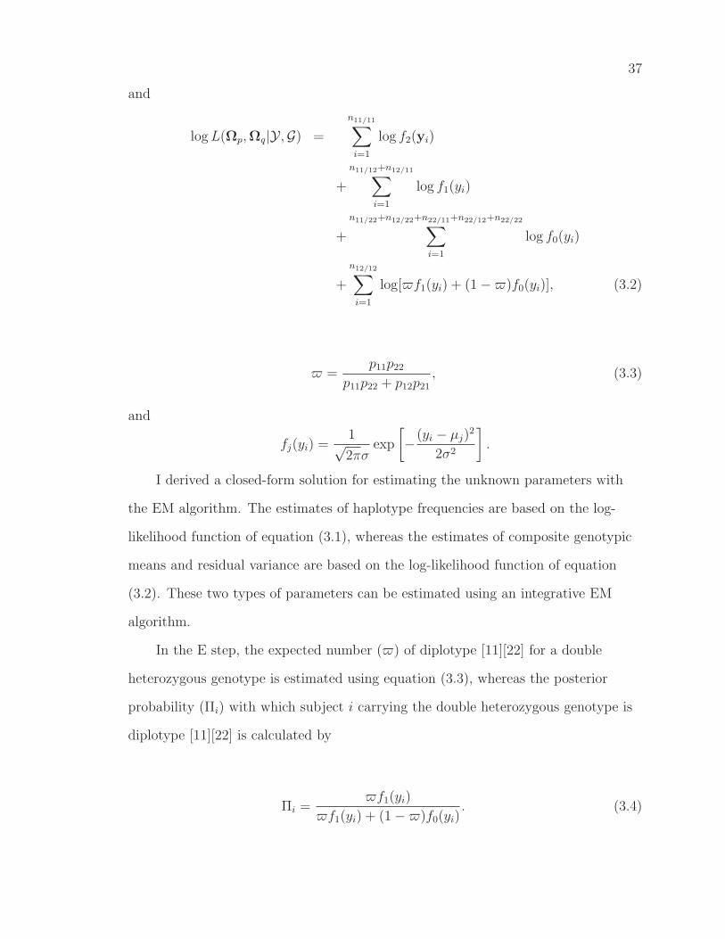
37
and
logL(Ωp,Ωq|Y ,G) =
n11/11∑
i=1
log f2(yi)
+
n11/12+n12/11∑
i=1
log f1(yi)
+
n11/22+n12/22+n22/11+n22/12+n22/22∑
i=1
log f0(yi)
+
n12/12∑
i=1
log[f1(yi) + (1 −)f0(yi)], (3.2)
=p11p22
p11p22 + p12p21
, (3.3)
and
fj(yi) =1√2πσ
exp
[−(yi − µj)
2
2σ2
].
I derived a closed-form solution for estimating the unknown parameters with
the EM algorithm. The estimates of haplotype frequencies are based on the log-
likelihood function of equation (3.1), whereas the estimates of composite genotypic
means and residual variance are based on the log-likelihood function of equation
(3.2). These two types of parameters can be estimated using an integrative EM
algorithm.
In the E step, the expected number () of diplotype [11][22] for a double
heterozygous genotype is estimated using equation (3.3), whereas the posterior
probability (Πi) with which subject i carrying the double heterozygous genotype is
diplotype [11][22] is calculated by
Πi =f1(yi)
f1(yi) + (1 −)f0(yi). (3.4)
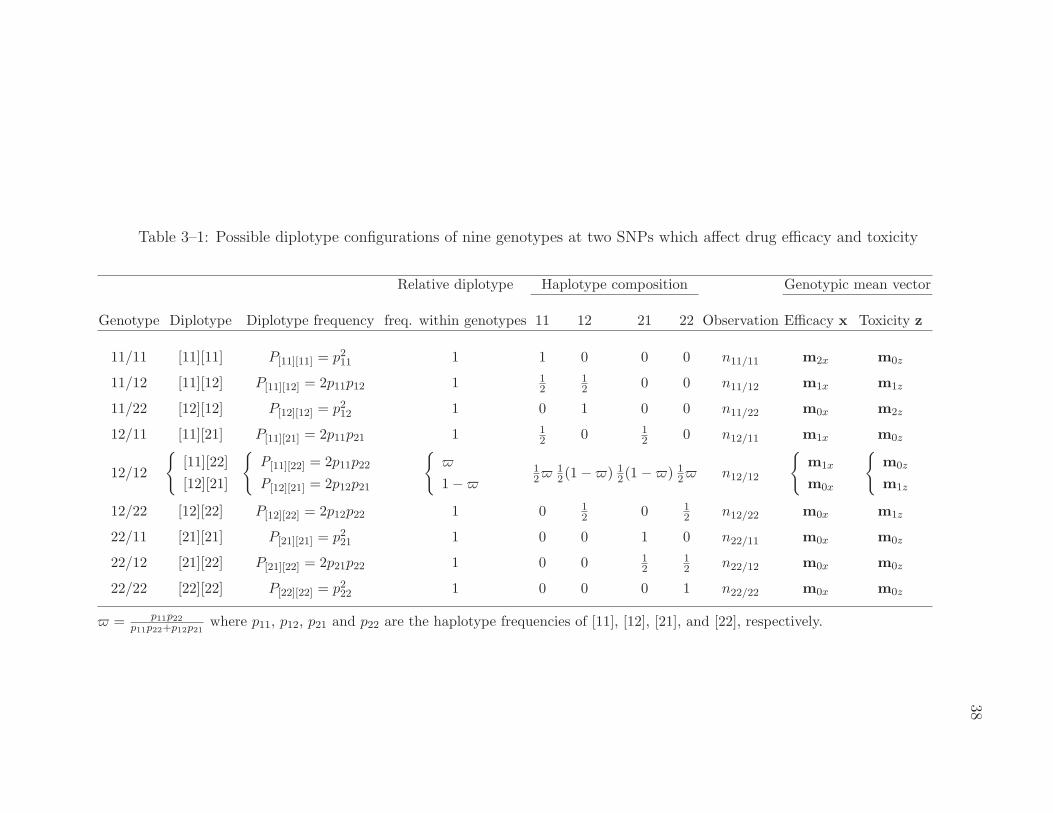
38
Table 3–1: Possible diplotype configurations of nine genotypes at two SNPs which affect drug efficacy and toxicity
Relative diplotype Haplotype composition Genotypic mean vector
Genotype Diplotype Diplotype frequency freq. within genotypes 11 12 21 22 Observation Efficacy x Toxicity z
11/11 [11][11] P[11][11] = p211 1 1 0 0 0 n11/11 m2x m0z
11/12 [11][12] P[11][12] = 2p11p12 1 12
12 0 0 n11/12 m1x m1z
11/22 [12][12] P[12][12] = p212 1 0 1 0 0 n11/22 m0x m2z
12/11 [11][21] P[11][21] = 2p11p21 1 12 0 1
2 0 n12/11 m1x m0z
12/12
[11][22]
[12][21]
P[11][22] = 2p11p22
P[12][21] = 2p12p21
1 − 12 1
2(1 − ) 12(1 − ) 1
2 n12/12
m1x
m0x
m0z
m1z
12/22 [12][22] P[12][22] = 2p12p22 1 0 12 0 1
2 n12/22 m0x m1z
22/11 [21][21] P[21][21] = p221 1 0 0 1 0 n22/11 m0x m0z
22/12 [21][22] P[21][22] = 2p21p22 1 0 0 12
12 n22/12 m0x m0z
22/22 [22][22] P[22][22] = p222 1 0 0 0 1 n22/22 m0x m0z
= p11p22
p11p22+p12p21where p11, p12, p21 and p22 are the haplotype frequencies of [11], [12], [21], and [22], respectively.

39
In the M step, the probabilities calculated in the previous iteration are used to
estimate the haplotype frequencies using
p11 =2n11/11 + n11/12 + n12/11 +n12/12
2n, (3.5)
p12 =2n11/22 + n11/12 + n12/22 + (1 −)n12/12
2n, (3.6)
p21 =2n22/11 + n12/11 + n22/12 + (1 −)n12/12
2n, (3.7)
p22 =2n22/22 + n22/12 + n12/22 +n12/12
2n, (3.8)
The quantitative genetic parameters are estimated using
µ2 =
∑n11/11
i=1 yi
n11/11
, (3.9)
µ1 =
∑ni=1 yi +
∑n12/12
i=1 Πiyi
n+∑n12/12
i=1 Πi
, (3.10)
µ0 =
∑ni=1 yi +
∑n12/12
i=1 (1 − Πi)yi
n+∑n12/12
i=1 (1 − Πi), (3.11)
σ2 =1
n
n11/11∑
i=1
(yi − µ2)2 +
n∑
i=1
(yi − µ1)2 +
n∑
i=1
(yi − µ0)2
+
n12/12∑
i=1
[Πi(yi − µ1)
2 + (1 − Πi)(yi − µ0)2] , (3.12)
where n = n11/12 + n12/11 and n = n11/22 + n12/22 + n22/11 + n22/12 + n22/22. Iterations
including the E and M steps are repeated among equations (3.4)–(3.12) until the
estimates of the parameters converge to stable values.
3.3 An Integrative Sequence and Functional Mapping Framework forDrug Efficacy and Toxicity
3.3.1 The Multivariate Normal Distribution
Efficacy and toxicity describe how patients respond to different doses or
concentrations of drugs. Statistically, these represent a longitudinal problem whose
underlying genetic determinants can be mapped using the functional mapping
strategy. Here, I integrate the ideas for sequence mapping and functional mapping

40
to directly characterize DNA sequence variants that are responsible for efficacy and
toxicity processes.
Consider the same sample as described above in which population genetic
parameters for SNPs have been defined. For each patient, drug effects are measured
at C hallmark dose or concentration levels. While a drug is expected to display
favorable effects, it may also be toxic. In this study, some typical physiological
parameters reflecting both efficacy and toxicity are longitudinally measured. Let
xi = [xi(1), · · · , xi(C)] be the efficacy effect vector and zi = [zi(1), · · · , zi(C)] be
the toxicity effect vector for a drug administrated to patient i. I use yi = (xi, zi)
to denote the joint vector combining these two types of drug response. Because the
phenotypic measurements of drug efficacy and toxicity are continuously variable, it
is reasonable to assume that y follows a multivariate normal distribution, as used in
general quantitative genetic studies (Lynch and Walsh 1998).
To jointly map the efficacy and toxicity, two log-likelihood functions described
in equations (3.1) and (3.2) should be constructed for observed SNP marker and
longitudinal phenotypic data. The only difference from single trait mapping is
that the log-likelihood function (3.2) needs to incorporate a multivariate normal
distribution for patient i who carries composite genotype j, expressed as
fj(yi;mj,Σ) =1
(2π)C |Σ|1/2exp
[−1
2(yi − mj)Σ
−1(yi − mj)T
], (3.13)
where yi = [xi(1), · · · , xi(C), zi(1), · · · , zi(C)] is a 2C-dimensional vector
of observations for efficacy and toxicity measured at C dosages and mj =
[µjx(1), · · · , µjx(C), µjz(1), · · · , µjz(C)] is a vector of expected values for com-
posite genotype j at different doses. At a particular dose c, the relationship between
the observation and expected mean can be described by a linear regression model,
xi(c) =J∑
j=1
ξijµjx(c) + eix(c), (3.14)

41
zi(c) =J∑
j=1
ζijµjz(c) + eiz(c), (3.15)
where ξij and ζij are the indicator variables denoted as 1 if a particular composite
genotype j is considered for individual i and 0 otherwise, J is the number of
composite genotypes and eix(c) and eiz(c) are the residual errors that are iid
normal with the mean of zero and the variances of σ2x(c) and σ2
z(c), respectively.
The errors at two different doses, c1 and c2, are correlated with the covariances
of σx(c1, c2) for efficacy, σz(c1, c2) for toxicity and σxz(c) and σxz(c1, c2) between
efficacy and toxicity. All these variances and covariances comprise the structure of
the (co)variance matrix Σ in equation (3.13), expressed as
Σ =
Σx Σxz
Σzx Σz
, (3.16)
where Σx and Σz are composed of σ2x(c) and σx(c1, c2), and σ2
z(c) and σz(c1, c2)
(1 ≤ c1, c2 ≤ C), respectively; and Σxz and Σzx are composed of σxz(c) and
σxz(c1x, c2z) (1 ≤ c1x 6= c2z ≤ C), and σzx(c) and σxz(c1z, c2x) (1 ≤ c1z 6= c2x ≤ C),
respectively.
To solve the likelihood functions implemented with response data measured
at multiple doses, one can extend the traditional interval mapping approach to
accommodate the multivariate nature of dose-dependent traits. However, this
extension is limited in two aspects: (1) Individual expected means of different
composite genotypes at all dose and all elements in the matrix Σ need to be
estimated, resulting in substantial computational difficulties when the vector and
matrix dimension is large; (2) The result from this approach may not be clinically
meaningful because the underlying medical principle for drug response is not
incorporated. Thus, some clinically interesting questions cannot be asked and
answered.

42
3.3.2 The Mapping Framework
Wu et al. (2002b, 2004a, 2004b) and Ma et al. (2002) have constructed a novel
statistical framework for functional mapping of QTL that affect growth curves.
Here, this framework is extended to jointly model two different longitudinal traits,
aimed at simultaneously characterizing the genetic variants responsible for efficacy
and toxicity. Two tasks are taken within this framework by modelling the mean
vector and the covariance matrix.
Modelling the mean vector: The dose-dependent expected values of
composite genotype j can be modelled for drug efficacy by the sigmoid Emax
model (Giraldo 2003) and for drug toxicity by the power function (McClish and
Roberts 2003). The Emax model postulates the following relationship between drug
concentration (C) and drug effect (µ):
µjx(C) = E0j +EmaxjC
Hj
ECHj
50j + CHj
, for composite genotype j, (3.17)
where E0 is the constant or baseline value for the drug response parameter, Emax is
the asymptotic (limiting) effect, EC50 is the drug concentration that results in 50%
of the maximal effect, and H is the slope parameter that determines the slope of the
concentration-response curve. Drug toxicity is described by the power function of
dose expressed as
µjz(C) = αjCβj , for composite genotype j, (3.18)
where β determines the shape of the dose-response relationship and α adjusts the
dose-related gain to which that shape conforms.
It is possible that efficacy and toxicity have different reference haplo-
types, so their composite genotypes should be treated differently. As a result,
equations (3.17) and (3.18) together contain 6 curve parameters for a defined
composite genotype j1 for efficacy and j2 for toxicity, which are arrayed by

43
Ωmj1j2= (E0j1 ,Emaxj1 ,EC50j1 ,Hj1 , αj2 , βj2). If different composite genotypes
have different combinations of these parameters, this implies that this sequence
plays a role in governing the differentiation of efficacy and toxicity. Thus, by testing
for the difference of Ωmj1j2among different genotypes, I can determine whether
there exists a specific sequence variant that confers an effect on these two drug
responses.
Modelling the structure of the covariance matrix: Many statistical
approaches have been proposed to model the structure of the covariance matrix
for longitudinal traits measured at multiple time points (Diggle et al. 2002). Here,
the matrix-structuring models will be derived on the basis of a commonly used
approach, structured antedependence (SAD) (Zimmerman and Nunez-Anton 2001).
According to the SAD model, an observation at a particular dosage c depends
on the previous ones, with the degree of dependence decaying with time lag. For
drug efficacy and toxicity, the dose-dependent residual errors for subject i described
by Equations (3.14) and (3.15) can be expressed, in terms of the first-order SAD
(SAD(1)) model, as
eix(c) = φxeix(c− 1) + ϕxeiz(c− 1) + ǫix(c),
eiz(c) = φzeiz(c− 1) + ϕzeix(c− 1) + ǫiz(c), (3.19)
where φx (or φz) and ϕx (or ϕz) are the unrestricted antedependence parameters
induced by trait x (or z) itself and by the other trait z (or x), respectively, and
ǫxi(c) and ǫxi(c) are the “innovation” errors for the two traits, respectively, normally
distributed as N(0, ν2x(c)) and N(0, ν2
z (c)) (Nunez-Anton and Zimmerman 2000;
Zimmerman and Nunez-Anton 2001). The bivariate SAD(1) model for subject i
described by equation (3.20) can be expressed in matrix notation as
ei = Φ−1εi, (3.20)

44
where ei = e1(1), · · · , ei(C)T, εi = ǫi(1), · · · , ǫi(C)T, and
Φ =
Φx Φxz
Φzx Φz
,
Φx =
1 0 0 · · · 0
−φx 1 0 · · · 0
0 −φx 1 · · · 0
0 0 −φx · · · 0
......
.... . .
...
0 0 0 · · · 1
, Φz =
1 0 0 · · · 0
−φz 1 0 · · · 0
0 −φz 1 · · · 0
0 0 −φz · · · 0
......
.... . .
...
0 0 0 · · · 1
,
Φxz =
0 0 0 · · · 0
−ψx 0 0 · · · 0
0 −ψx 0 · · · 0
0 0 −ψx · · · 0
......
.... . .
...
0 0 0 · · · 0
, Φzx =
0 0 0 · · · 0
−ψz 0 0 · · · 0
0 −ψz 0 · · · 0
0 0 −ψz · · · 0
......
.... . .
...
0 0 0 · · · 0
.
The covariance matrix of ei under the bivariate SAD(1) model (21) can be
obtained as
Σ = Φ−1Σǫ(Φ−1)T, (3.21)
where
Σǫ =
Σǫx Σǫxz
Σǫzx Σǫz
,

45
Σǫx =
ν2x(1) 0 0 · · · 0
0 ν2x(2) 0 · · · 0
......
.... . .
...
0 0 0 · · · ν2x(C)
, Σǫz =
ν2z (1) 0 0 · · · 0
0 ν2z (2) 0 · · · 0
......
.... . .
...
0 0 0 · · · ν2z (C)
.
and
Σǫxz = Σǫzx =
νxνzρ(1) 0 0 · · · 0
0 νxνzρ(2) 0 · · · 0
......
.... . .
...
0 0 0 · · · νxνzρ(C)
.
In this modelling, the innovative variance is assumed to be constant over different
dosages. As shown by Jaffrezic et al. (2003), the SAD(1) model with this assump-
tion can still allow for both the variance and correlation to change with the dose
level. In addition, I assume that the correlation (ρ) in innovative errors between the
two traits x and z is stable over dosage. With these assumptions, I need to estimate
an array of parameters contained in Ωv = (ν2x, ν
2z , φx, φz, ϕx, ϕz, ρ) that model the
structure of the covariance matrix under the SAD model.
In the context of the bivariate SAD model, the cross-correlation functions
can be proven to be asymmetrical, i.e., Corrxz(c1x, c2z) 6= Corrzx(c1z, c2x). This
favorable feature of the bivariate SAD model makes it useful for understanding the
genetic correlation between different traits. In practice, innovative variance and
correlation can be modelled by a polynomial and exponential function, respectively
(Nunez-Anton and Zimmerman 2000).
3.3.3 Computational Algorithm
I implemented the EM algorithm, originally proposed by Dempster et al.
(1977), to obtain the maximum likelihood estimates (MLEs) of three groups of
unknown parameters in the integrated sequence and function mapping model,

46
that is, the marker population parameters (Ωp), the curve parameters (Ωmj1j2)
that model the mean vector, and the parameters (Ωv) that model the structure of
the covariance matrix. These unknowns are denoted by Ω = (Ωp,Ωmj1j2,Ωv). A
detailed description of the EM algorithm was given in Wu et al. (2002b, 2004b) and
Ma et al. (2002).
As described for single trait mapping, I implement the E step to calculate the
expected number () of diplotype [11][22] contained in the double heterozygote
12/12 and the posterior probability (Πi) of double heterozygotic patient i who
carries diplotype [11][22]. In the M step, I use the calculated and Πi values to
estimate the haplotype frequencies using equations (3.5)–(3.8). But in this step, I
encounter a considerable difficulty in deriving the log-likelihood equations for Ωmj1j2
and Ωv because they are contained in complex nonlinear equations. Zhao et al.
(2004) implemented the simplex method as advocated by Nelder and Mead (1965)
to the estimation process of functional mapping, which can strikingly increase
computational efficiency. In this chapter, the simplex algorithm is embedded in the
EM algorithm above to provide simultaneous estimation of haplotype frequencies
and curve parameters and matrix-structuring parameters.
3.3.4 Model for an Arbitrary Number of SNPs
The idea for sequencing drug response has been described for a two-SNP
model. It is possible that the two-SNP model is too simple to characterize genetic
variants for variation in drug response. I have extended this model to include an
arbitrary number of SNPs whose sequences are associated with drug response
variation. A key issue for the multi-SNP sequencing model is how to distinguish
among 2r−1 different diplotypes for the same genotype heterozygous at r loci. The
relative frequencies of these diplotypes can be expressed in terms of haplotype
frequencies. The integrative EM algorithm can be employed to estimate the MLEs
of haplotype frequencies. Bennett (1954) provided a general formula for expressing

47
haplotype frequencies in terms of allele frequencies and linkage disequilibria of
different orders. The MLEs of the latter can be obtained by solving a system of
equations.
3.4 Hypothesis Tests
Different from traditional mapping approaches, the functional mapping for
function-valued traits allows for tests of a number of biologically or clinically mean-
ingful hypotheses. These hypotheses include tests for the existence of significant
DNA sequence variants, for the genetic effect on the maximal (asymptotic) effect
(Emax), for the drug concentration that results in 50% of the maximal effect, and for
the slopes that determines the steepness of the concentration-response curve.
The existence of specific genetic variants affecting drug efficacy and toxicity
can be tested by formulating null and alternative hypotheses,
H0 : Ωmj1j2≡ Ωm, j1, j2 = 2, 1, 0
H1 : at least one of the equalities above does not hold,
(3.22)
where H0 corresponds to the reduced model, in which the data can be fit by a
single drug response curve, and H1 corresponds to the full model, in which there
exist different dynamic curves to fit the data. The test statistic for testing the
hypotheses in equation (3.23) is calculated as the log-likelihood ratio (LR) of the
reduced to the full model:
LR = −2[logL(Ω|y,G) − logL(Ω|y,G)], (3.23)
where Ω and Ω denote the MLEs of the unknown parameters under H0 and
H1, respectively. The LR is asymptotically χ2-distributed with 12 degrees of
freedom. An empirical approach for determining the critical threshold is based on
permutation tests, as advocated by Churchill and Doerge (1994). By repeatedly
shuffling the relationships between marker genotypes and phenotypes, a series of the

48
maximum log-likelihood ratios are calculated, from the distribution of which the
critical threshold is determined.
I can also test for the significance of the genetic effect on drug efficacy or
toxicity at a particular concentration level (c∗) of interest, expressed as
H0 : µj1x(c∗) = µx(c
∗), µj2z(c∗) = µz(c
∗)
H1 : At least one of the eqaulities above does not hold,
(3.24)
which is equivalent to testing the difference of the full model with no restriction and
the reduced model with a restriction in H0. Similar restrictions can be taken to test
the genetic effect on individual curve parameters, such as Emax, EC50, H, α and β.
The tests of these parameters are important for the design of personalized drugs to
control particular diseases.
3.5 Results
I perform Monte Carlo simulation experiments to examine the statistical
properties of the model proposed for genetic mapping of drug efficacy and toxicity.
The simulation will be based on the bivariate SAD(1) model (equation 3.21). For
computational simplicity, I only considers the antedependence parameters induced
by the trait itself, i.e., setting ϕx = ϕz = 0. I randomly choose 200 individuals from
a human population at Hardy-Weinberg equilibrium with respect to haplotypes.
Let us consider two SNPs with allele frequencies and linkage disequilibrium given
in Table 3-1. The diplotypes derived from four haplotypes at these two SNPs affect
drug efficacy and toxicity. Here I assume that these two types of drug response have
different reference haplotypes, i.e., 11 for efficacy and 12 for toxicity. Thus, each
drug response corresponds to a different set of three composite genotypes.
The efficacy (E0, Emax, EC50, H) and toxicity curve parameters (α and β) for
the respective three composite genotypes, given in Table 3-1, are determined in
the ranges of empirical estimates of these parameters from pharmacological studies

49
(Sowinski et al. 1995; McClish and Roberts 2003). I use a general clinical design,
with drug effects measured at 9 different concentrations of drug, 0, 5, 10, 15, 20, 25,
30, 35 and 40, expressed as c = 1, 2, · · · , 9 (Figure 3-1), for this simulation study.
Using the genetic variance due to the composite genotypic difference in the area
under curve, I calculate the residual variances under different heritability levels
(H2 = 0.1 and 0.4). These residual variances, plus given residual correlations, form
a structured residual covariance matrix Σ (equation 3.22). The phenotypic values of
drug effect for 200 random patients are simulated by the summations of genotypic
values predicted by the curves and residual errors following multivariate normal
distributions, with MVN(0,Σ).
The population genetic parameters of the SNPs can be estimated with rea-
sonably high precision using the closed-form solution approach (Table 3-2). The
estimates of these parameters are only dependent on sample size and are not related
to the size of heritability. Figure 3-1 illustrates different forms of the drug efficacy
and toxicity curves from the three composite genotypes with a comparison between
the hypothesized and estimated curves. The estimated curves are consistent with
the hypothesized curves, especially when the heritability is larger (0.4), suggesting
that the model can provide reasonable estimates of drug response curves. The
parameters for the efficacy and toxicity models of each composite genotype can be
estimated accurately and precisely (Table 3-2). As expected, the estimation preci-
sion (assessed by square root of MSEs) increases remarkably when the heritability
increases from 0.1 to 0.4. The estimates of the SAD parameters that model the
structure of the covariance matrix Σ also display reasonably high precision (Table
3-2). But it seems that their estimation precision is independent of the size of
heritability.
In each of 100 simulations, I calculate the log-likelihood ratios (LR) for the
hypothesis test of the presence of a genetic variant affecting both drug responses.

50
Table 3–2: Maximum likelihood estimates of SNP population genetic parameters (allelefrequencies and linkage disequilibrium), the curve parameters and matrix-structuring pa-rameters for efficacy and toxicity responses. The numbers in parentheses are the squareroot of MSEs of the estimates.
Composite HeritabilityParameters genotype True value 0.1 0.4
Population genetic parameters
p(1)1 0.60 0.60(0.02) 0.60(0.02)
p(2)1 0.70 0.70(0.02) 0.70(0.02)
D 0.08 0.08(0.01) 0.08(0.02)
Curve parameters: Efficacy
E0 [11][11] 0.27 0.27(0.01) 0.27(3e-3)[11][11] 0.25 0.25(0.01) 0.25(3e-3)[11][11] 0.23 0.23(0.01) 0.23(4e-3)
Emax [11][11] 0.90 0.93(0.11) 0.92(0.08)[11][11] 0.85 0.85(0.12) 0.84(0.06)[11][11] 0.80 0.80(0.16) 0.79(0.11)
EC50 [11][11] 24.00 25.57(6.14) 24.78(3.66)[11][11] 25.00 25.46(7.94) 25.17(4.98)[11][11] 26.00 27.53(14.67) 26.26(10.71)
H [11][11] 1.10 1.10(0.09) 1.10(0.07)[11][11] 1.00 1.03(0.11) 1.04(0.05)[11][11] 0.90 0.94(0.12) 0.93(0.08)
Curve parameters: Toxocity
α [12][12] 0.10 0.10(0.02) 0.10(0.01)[12][12] 0.13 0.13(0.01) 0.13(2e-3)[12][12] 0.16 0.16(4e-3) 0.16(2e-3)
β [12][12] 0.60 0.60(0.08) 0.60(0.04)[12][12] 0.50 0.50(0.01) 0.50(6e-3)[12][12] 0.40 0.40(8e-3) 0.40(4e-3)
Matrix-structuring parameters
φx 0.30 0.28(0.04) 0.29(0.02)φz 0.40 0.39(0.03) 0.40(0.02)ρ 0.70 0.70(0.01) 0.70(0.01)ν2
x 8e-3 8e-3(3e-4)1e-3 1e-3(5e-5)
ν2z 3e-3 3e-3(1e-4)
6e-4 6e-3(2e-5)

51
The LR values in each simulation under both heritability levels are strikingly higher
than the critical threshold estimated from 100 replicates of simulations under the
null hypothesis that there is no drug response-associated genetic variant. This
suggests that this model has enough power to detect the genetic variant under given
SNPs, curve and matrix-structuring parameters for the simulation. With the same
set of simulated data, the power to detect significant genetic variants is reduced by
∼10% when drug efficacy or toxicity is modelled separately.
I carry out an additional simulation study to examine the statistical behavior
of this model when 3 different SNPs are used. This 3-SNP model uses the same
parameters as assumed under the 2-SNP model, except for the inclusion of more
SNPs. The results from the 3-SNP model are broadly concordant with those from
the 2-SNP model (results not given), although more population genetic parameters
need to be estimated in the former than latter.
3.6 Discussion
Drug response is complex in nature. First, no drug is universally effective;
efficacy rates for drug therapy of most diseases ranges from 25 to 80% (Spear et
al. 2001). Second, all drugs that produce an efficacious response may also produce
adverse effects (Johnson 2002). Third, both drug efficacy and toxicity that vary in
human populations are determined by multiple genetic and environmental factors
that interact with one another in complicated ways (Watters and Mcleod 2003). It
is possible that the genetic polymorphisms associated with a favorable response to
therapy may or may not be associated with toxicity risk (Nebert 1997; Wilson et al.
2001).
The complexity of drug response is enforced by its dynamic characteristic with
high dimension and correlated structure. The genetic analysis of drug response,
therefore, needs more sophisticated statistical tools that have capacity to extract
useful information from longitudinal data. In this chapter, I have proposed a

52
novel statistical model for characterizing the genetic variants that govern drug
response in a human population. This model is constructed with a finite mixture
model framework founded on the tenets of the sequence (Lin et al. 2005) and
functional mapping (Ma et al. 2002; Wu et al. 2002b, 2004a, 2004b). This model
has particular power to discern the discrepancy between the genetic mechanisms
underlying drug efficacy and toxicity.
Compared to traditional genetic mapping approaches, this model is both
genetically and statistically merited. It offers a direct tool to detect DNA sequences
that code drug response. The haplotype map or HapMap constructed from single
nucleotide polymorphisms (SNPs) (The International HapMap Consortium 2003)
makes the application of this model practically possible. In particular, I adopt
clinally meaningful mathematical functions (Giraldo 2003; McClish and Roberts
2003) when modelling dose-dependent drug response. This has two advantages.
First, it facilitates statistical analysis and strengthens power to detect significant
genetic variants because fewer parameters are needed to be estimated, as opposed
to traditional multivariate analysis. Second, the results it produces are close to
biological realm given that the mathematical functions used are founded on a firm
understanding of pharmacology (reviewed in Derendorf and Meibohm 1999). The
statistical power of this model is further increased by the attempt to structure the
covariance matrix with autoregressive models (Diggle et al. 2002).
I have performed different simulation studies to investigate the statistical
behavior of this model. The results suggest that it can provide accurate and precise
estimates of the response curves for both efficacy and toxicity even when the
heritability is modest. Different drug response curves, as simulated for different
composite genotypes (Figure 3-1), can offer scientific guidance for determining the
optimal dosage that balances favorable efficacy and unfavorable toxicity based on
individual’s genetic background. It should be noted that this model was derived
53
on the basis of a simple clinical design in which a single cohort is assumed, with
equally concentration intervals for every patient. This model can be extended to
a case-control study by allowing haplotype frequencies and haplotype effects to be
different between the case and control groups. A series of hypothesis tests regarding
between-group differences can be formulated to detect specific haplotypes that are
responsible for drug response. My model can also be extended to consider various
measurement schedules, in particular with uneven concentration lags varying from
patient to patient. For these irregular measurement schedules, it is needed to
formulate individualized likelihood functions when the mean vector and covariance
matrix are modelled (see Nunez-Anton and Woodworth 1994).
In coupling with continuing advances in molecular biological technology and
the availability of a complete reference sequence of the entire human genome (Patil
et al. 2001; Dawson et al. 2002; Gabriel et al. 2002), this model will assist in the
discovery and characterization of the genes that influence drug response, and lead
to a better understanding of how genes function and the subsequent development of
new approaches to the diagnosis and treatment of common diseases by medications.
Once the network of genes that govern drug responses in humans is defined, it will
then be possible to more accurately optimize drug therapy based on each patient’s
ability to metabolize, transport and respond to medications.

54
0 10 20 30 400
20
40
60
80
100
Drug concentration (mcg)
Effi
cacy
(%
)
A
0 10 20 30 400
20
40
60
80
100
Drug concentration (mcg)
Tox
icity
(%
)
B
0 10 20 30 400
20
40
60
80
100
Drug concentration (mcg)
Effi
cacy
(%
)
C
0 10 20 30 400
20
40
60
80
100
Drug concentration (mcg)
Tox
icity
(%
)
D
Figure 3–1: Estimated response curves (dash) each corresponding to one of threecomposite genotypes under the heritability (H2) of 0.1 (A and B) and 0.4 (C andD), in a comparison with the hypothesized curves (solid) used to simulate indi-vidual curves for drug efficacy (A and C) and toxicity (B and D), respectively.Nine different concentrations, 0, 5, 10, 15, 20, 25, 30, 35 and 40, at which responsesare measured, are used. The consistency between the estimated and hypothesizedcurves suggests that this model can provide the precise estimation of the geneticcontrol over response curves in patients. The homozygote composed of two ref-erence haplotypes is [11][11] for efficacy and [12][12] for toxicity (blue), the het-erozygote composed of one reference and one non-reference haplotype is [11][11]for efficacy and [12][12] for toxicity (red), and the homozygote composed of twonon-reference haplotypes is [11][11] for efficacy and [12][12] for toxicity (green).

CHAPTER 4MODEL FOR DETECTING SEQUENCE-SEQUENCE INTERACTIONS FOR
COMPLEX DISEASES
4.1 Introduction
Interactions between different genes, coined the epistasis, have long been recog-
nized to play a central role in shaping the genetic architecture of a quantitative
trait (Whitlock et al. 1995; Wolf et al. 2000). Recent genetic studies from vast
quantities of molecular data have also indicated that epistasis is of paramount
importance in the pathogenesis of most common human diseases, such as cancer
or cardiovascular disease (Moore 2003). The evidence for this is the nonlinear
relationship detected between genotype and phenotype. The decipherment of in-
terconnected networks of genes and their associations with disease susceptibility
has become a pressing demand for a detailed understanding of the genetic basis for
disease processes.
The most common and powerful approaches for detecting genome-wide
epistasis are based on genetic mapping that associates phenotypic variation of
a trait with a linkage map constructed by polymorphic markers (Lander and
Botstein 1989). Significant associations imply the existence of the underlying loci
(called quantitative trait loci or QTL) that are responsible for variation in the
trait. Epistatic QTL are considered to occur if the effect of one QTL depends on
the expression of other QTL. While traditional genetic mapping can only make
an indirect inference about QTL actions and interactions, a newly developed
mapping approach based on the haplotype map (HapMap) constructed from single
nucleotide polymorphisms (SNPs) (The International HapMap Consortium 2003)
can directly characterize specific DNA sequence variants for a phenotype (Liu et al.
55

56
2004). Beyond hypothesized chromosomal segments identified by QTL mapping,
this so-called sequence mapping approach, relied upon the the characterization of
SNPs from the entire human genome, can probe concrete nucleotoxic sites, i.e.,
quantitative trait nucleotides (QTN), that contribute to variation in a quantitative
trait.
In this chapter, I extend the previous statistical model to determine the
epistasis between specific DNA sequences responsible for the phenotypic variation
of disease risk. This extended model is derived through the analysis of pair-wise
multilocus haplotypes constructed by a finite number of tag SNPs. I derived a
closed form solution for estimating the action and interaction effects of haplotypes,
haplotype frequencies, allele frequencies and the degrees of LD of various orders
among tag SNPs underlying the disease. Simulation studies were performed to test
the statistical behavior of this haplotype-based epistatic mapping model. I used a
worked example for a human obesity study to demonstrate the usefulness of the
model.
4.2 The Model
4.2.1 Notation
Consider a natural human population at Hardy-Weinberg equilibrium from
which a random sample of size n is drawn. In order to identify DNA sequences
responsible for a complex disease, I genotype a number of SNPs genomewide and
construct a haplotype map. Recent molecular surveys suggest that the human
genome contains many discrete haplotype blocks that are sites of closely located
SNPs (Daly et al. 2001; Patil et al. 2001; Gabriel et al. 2002). Each block may
have a few common haplotypes which account for a large proportion of chromoso-
mal variation. Between adjacent blocks there are large regions, called hotspots, in
which recombination events occur with high frequencies. Several algorithms have
been developed to identify a minimal subset of SNPs, i.e., “tagging” SNPs, that

57
can characterize the most common haplotypes (Zhang et al. 2002b, 2002c; Kimmel
and Shamir 2005). In this study, I assume that the number and type of tagging
SNPs within each haplotype block has been determined. The rationale behind
the epistatic model being developed is that the effect of a given DNA sequence in
one haplotype block on a complex disease is masked or enhanced by one or more
sequences in other blocks.
Suppose there are R and S (R,S > 1) tagging SNPs for two arbitrary
haplotype blocks R and S, respectively. Two alleles of a tag SNP r or s from block
R or S can be denoted by U rkr
(kr = 1, 2; r = 1, · · ·R) and V sls(ls = 1, 2; s = 1, · · ·S),
respectively. I use pRkrand pSls to denote allele frequencies at the corresponding
SNP. All the SNPs within each of the two blocks form 2R or 2S possible haplotypes
expressed as U1k1U2
k2· · ·UR
kRand V 1
l1V 2
l2· · ·V S
lS, respectively. The corresponding
haplotype frequencies within each block are denoted by pRk1k2···kRand pSl1l2···lS
,
which are composed of allele frequencies at each SNP and linkage disequilibria of
different orders among SNPs (Lynch and Walsh 1998). A general expression for
the relationships between haplotype frequencies and allele frequencies and linkage
disequilibria was given by Bennett (1954). Lou et al. (2003) derived a closed-form
EM algorithm to estimate haplotype frequencies, which can be further used to
estimate allele frequencies and linkage disequilibria based on these established
relationships.
The random combination of maternal and paternal haplotypes generates
2R−1(2R + 1) diplotypes expressed as [U1k1U2
k2· · ·UR
kR][U1
k′1U2
k′2· · ·UR
k′
R] (1 ≤ k1 ≤ k′1 ≤
2, · · · , 1 ≤ kR ≤ k′R ≤ 2) for block R and 2S−1(2S + 1) diplotypes expressed as
[V 1l1V 2
l2· · ·V S
lS][V 1
l′1V 2
l′2· · ·V S
l′S] (1 ≤ l1 ≤ l′1 ≤ 2, · · · , 1 ≤ lR ≤ l′R ≤ 2) for block S.
I use the brackets to separate maternal (former) and paternal haplotypes (latter)
for a given diplotype. Unless there are two or more SNPs that are heterozygous,
observable zygotic genotypes will be the same as diplotypes. Thus, the numbers

58
of zygotic genotypes, 3R or 3S, will be less than the number of diplotypes and
the difference between these two numbers is statistically viewed as missing data.
The observed zygotic genotypes are expressed as U1k1U1
k′1/U2
k2U2
k′2/ · · · /UR
kRUR
k′
Ror
V 1l1V 1
l′1/V 2
l2A2
l′2/ · · · /V S
lSV S
l′Sfor the two blocks, respectively. Let PR
[k1k2···kR][k′1k′
2···k′
R] and
PRk1k′
1/k2k′2/···/kRk′
Rdenote the diplotype and genotype frequencies, respectively, for
block R. The corresponding expressions are P S[l1l2···lR][l′1l′2···l
′
S ] and P Sl1l′1/l2l′2/···/lS l′S
for
block S.
Because phenotypic variation in a complex disease can be explained by
haplotype diversity, a particular haplotype can be assumed to be different from
other haplotypes for a given phenotype (Bader 2001). Liu et al. (2004) defined such
a distinct haplotype as reference haplotype. They further defined the diplotypes
formed by reference and/or non-reference haplotypes as composite genotypes.
Although it cannot be directly observed, the difference between the reference and
non-reference haplotypes can be inferred from observed zygotic genotypes with the
EM algorithm.
4.2.2 Epistatic Effects
Let A, A and B, B be the reference and non-reference haplotypes at block
R and S, respectively. In the given sample, these two blocks form nine different
composite genotypes expressed as AABB, AABB, AABB, AABB, AABB,
AABB, AABB, AABB and AABB. Traditional quantitative genetic theories
can be used to model the genetic effects of the composite genotypes (Lynch and
Walsh 1998). The genotypic value (µjRjS ) of a joint composite genotype at the two
haplotype blocks can be decomposed into nine different components as follows:
µjRjS = µ Overall mean (4.1)
+ (jR − 1)αR + (jS − 1)αS Additive effects
+ [1 − (jR − 1)2]βR + [1 − (jS − 1)2]βS Dominant effects
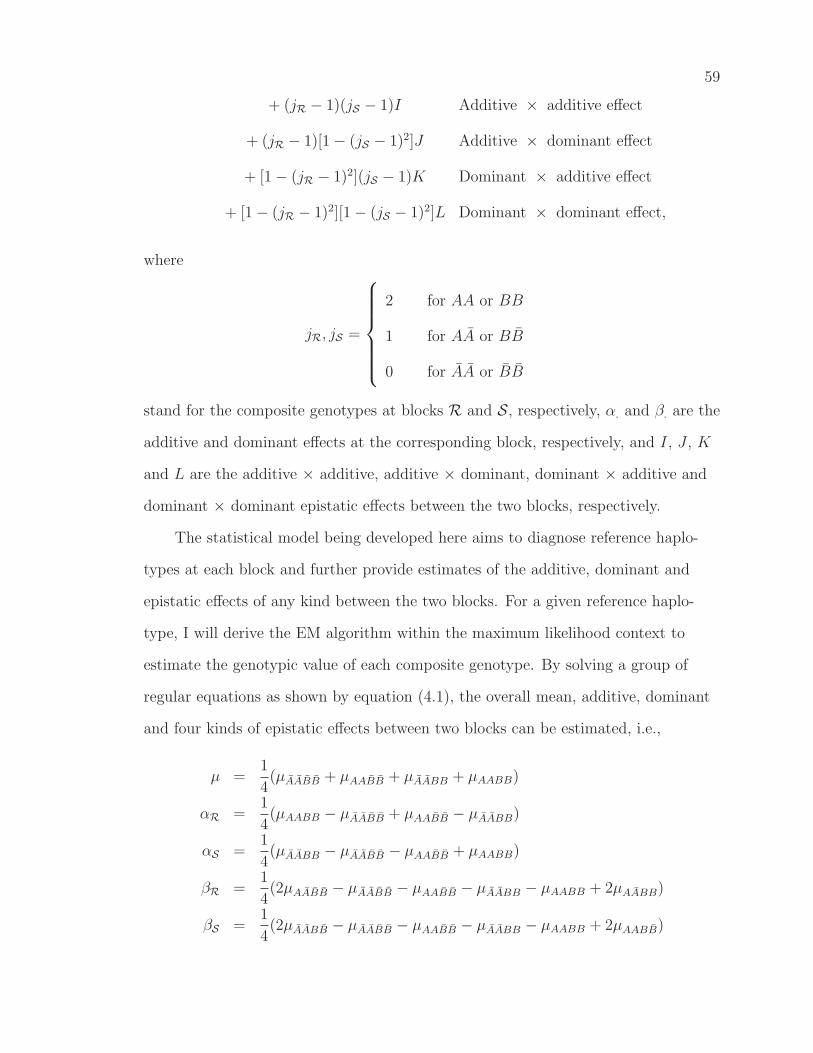
59
+ (jR − 1)(jS − 1)I Additive × additive effect
+ (jR − 1)[1 − (jS − 1)2]J Additive × dominant effect
+ [1 − (jR − 1)2](jS − 1)K Dominant × additive effect
+ [1 − (jR − 1)2][1 − (jS − 1)2]L Dominant × dominant effect,
where
jR, jS =
2 for AA or BB
1 for AA or BB
0 for AA or BB
stand for the composite genotypes at blocks R and S, respectively, α. and β. are the
additive and dominant effects at the corresponding block, respectively, and I, J , K
and L are the additive × additive, additive × dominant, dominant × additive and
dominant × dominant epistatic effects between the two blocks, respectively.
The statistical model being developed here aims to diagnose reference haplo-
types at each block and further provide estimates of the additive, dominant and
epistatic effects of any kind between the two blocks. For a given reference haplo-
type, I will derive the EM algorithm within the maximum likelihood context to
estimate the genotypic value of each composite genotype. By solving a group of
regular equations as shown by equation (4.1), the overall mean, additive, dominant
and four kinds of epistatic effects between two blocks can be estimated, i.e.,
µ =1
4(µAABB + µAABB + µAABB + µAABB)
αR =1
4(µAABB − µAABB + µAABB − µAABB)
αS =1
4(µAABB − µAABB − µAABB + µAABB)
βR =1
4(2µAABB − µAABB − µAABB − µAABB − µAABB + 2µAABB)
βS =1
4(2µAABB − µAABB − µAABB − µAABB − µAABB + 2µAABB)

60
I =1
4(µAABB − µAABB − µAABB + µAABB)
J =1
4(2µAABB − µAABB − 2µAABB + µAABB − µAABB + µAABB)
K =1
4(2µAABB − 2µAABB + µAABB + µAABB − µAABB − µAABB)
L =1
4(4µAABB + µAABB + µAABB + µAABB + µAABB − 2µAABB
−2µAABB − 2µAABB − 2µAABB) (4.2)
These estimates are the maximum likelihood estimates (MLEs) based on the
invariant property of the maximum likelihood method.
4.2.3 Likelihood Functions
This model is unique in that two different likelihood functions can be inte-
grated to estimate haplotype frequencies (population genetic parameters) and
genotypic values of composite genotypes and residual variance (quantitative ge-
netic parameters). For two different haplotype blocks R and S, between which no
linkage disequilibria exist (Daly et al. 2001; Gabriel et al. 2002), across-block hap-
lotype frequencies can be calculated as the product of the corresponding haplotype
frequencies from a different block, expressed as
p(k1k2···kR)(l1l2···lS) = pRk1k2···kRpSl1l2···lS
, (4.3)
where the parentheses are used to separate two different blocks for a given across-
block haplotype. With these across-block haplotype frequencies, expected across-
block diplotype frequencies and across-block genotype frequencies can be calculated,
respectively, under Hardy-Weinberg equilibrium.
With across-block diplotype and genotype frequencies, the likelihood function
based on across-block genotype observations, n = n(k1k′1/k2k′
2/···/kRk′
R)(l1l′1/l2l′2/···/lS l′S),
can be constructed. To simplify the presentation of my model, I will first assume
two tagging SNPs for each block. Table 4-1 lists all possible genotypes and diplo-
types as well as their frequencies at two SNPs genotyped from block R. Each

61
Table 4–1: Possible diplotype configurations of nine genotypes at two SNPs and their haplotype composition frequencies
Relative diplotype Haplotype composition
Genotype Diplotype Diplotype frequency freq. within genotypes U11 U2
1 U11 U2
2 U12 U2
1 U12 U2
2 Observation Genotypic mean
U11 U1
1 /U21 U2
1 [U11 U2
1 ][U11 U2
1 ] P[11][11] = p211 1 1 0 0 0 n11/11 µ2· = µ + a
U11 U1
1 /U21 U2
2 [U11 U2
1 ][U11 U2
2 ] P[11][12] = 2p11p12 1 12
12 0 0 n11/12 µ1· = µ + d
U11 U1
1 /U22 U2
2 [U11 U2
2 ][U11 U2
2 ] P[12][12] = p212 1 0 1 0 0 n11/22 µ0· = µ − a
U11 U1
2 /U21 U2
1 [U11 U2
1 ][U12 U2
1 ] P[11][21] = 2p11p21 1 12 0 1
2 0 n12/11 µ1· = µ + d
U11 U1
2 /U21 U2
2
[U1
1 U21 ][U1
2 U22 ]
[U11 U2
2 ][U12 U2
1 ]
P[11][22] = 2p11p22
P[12][21] = 2p12p21
π
1 − π12π 1
2(1 − π) 12(1 − π) 1
2π n12/12
µ1· = µ + d
µ0· = µ − a
U11 U1
2 /U22 U2
2 [U11 U2
2 ][U12 U2
2 ] P[12][22] = 2p12p22 1 0 12 0 1
2 n12/22 µ0· = µ − a
U12 U1
2 /U21 U2
1 [U12 U2
1 ][U12 U2
1 ] P[21][21] = p221 1 0 0 1 0 n22/11 µ0· = µ − a
U12 U1
2 /U21 U2
2 [U12 U2
1 ][U12 U2
2 ] P[21][22] = 2p21p22 1 0 0 12
12 n22/12 µ0· = µ − a
U12 U1
2 /U22 U2
2 [U12 U2
2 ][U12 U2
2 ] P[22][22] = p222 1 0 0 0 1 n22/22 µ0· = µ − a
π = p11p22
p11p22+p12p21where p11, p12, p21 and p22 are the haplotype frequencies of U1
1 U21 , U1
1 U22 , U1
2 U21 , and U1
2 U22 , respectively, and
µjR·=
∑jS=2jS=0 µjRjS .

62
diplotype is composed of two haplotypes, one from the mother and the other from
the father. The diplotype frequencies can be expressed in terms of the haplotype
frequencies (Table 4-1). The same genotype may contain two different diplotypes,
depending on its heterozygosity. Table 4-1 also gives the relative frequencies with
which a genotype carries a particular haplotype. Such relative frequencies will
be useful for partitioning observed genotypes into underlying diplotypes in the
construction of likelihood function based on the phenotype.
Considering two blocks R and S at the same time, I will have the joint
haplotype frequencies, arrayed by Ωp = (pRk1k2, pSl1l2
). The log-likelihood function of
these unknown haplotype frequencies given observed genotypes (n) can be written
as a multinomial form, i.e.,
logL(Ωp|n) ∝ (4.4)
22∑
k1=1
2∑
k2=1
2∑
l1=1
2∑
l2=1
n(k1k1/k2k2)(l1l1/l2l2)(log pRk1k2+ log pSl1l2
)
+2∑
k1=1
2∑
k2=1
2∑
l1=1
n(k1k1/k2k2)(l1l1/l2l′2)[2 log pRk1k2+ log (2pSl1l2
pSl1l′2)]
+2∑
k1=1
2∑
k2=1
2∑
l2=1
n(k1k1/k2k2)(l1l′1/l2l2)[2 log pRk1k2+ log (2pSl1l2
pSl′1l2)]
+2∑
k1=1
2∑
k2=1
n(k1k1/k2k2)(l1l′1/l2l′2)[2 log pRk1k2+ log (2pSl1l2
pSl′1l′2+ 2pSl1l′2
pSl1l′2)]
+2∑
k1=1
2∑
l1=1
2∑
l2=1
n(k1k1/k2k′2)(l1l1/l2l2)[log(2pRk1k2
pRk1k′2) + 2 log (pSl1l2
)]
+2∑
k1=1
2∑
l1=1
n(k1k1/k2k′2)(l1l1/l2l′2)[log(2pRk1k2
pRk1k′2) + log (2pSl1l2
pSl1l′2)]
+2∑
k1=1
2∑
l2=1
n(k1k1/k2k′2)(l1l′1/l2l2)[log(2pRk1k2
pRk1k′2) + log (2pSl1l2
pSl′1l2)]
+2∑
k1=1
n(k1k1/k2k′2)(l1l′1/l2l′2)[log(2pRk1k2
pRk1k′2) + log (2pSl1l2
pSl′1l′2+ 2pSl1l′2
pSl′1l2)]

63
+2∑
k2=1
2∑
l1=1
2∑
l2=1
n(k1k′1/k2k2)(l1l1/l2l2)[log(2pRk1k2
pRk′1k2
) + 2 log (pSl1l2)]
+2∑
k2=1
2∑
l1=1
n(k1k′1/k2k2)(l1l1/l2l′2)[log(2pRk1k2
pRk′1k2
) + log (2pSl1l2pSl1l′2
)]
+2∑
k2=1
2∑
l2=1
n(k1k′1/k2k2)(l1l′1/l2l2)[log(2pRk1k2
pRk′1k2
) + log (2pSl1l2pSl′1l2
)]
+2∑
k2=1
n(k1k′1/k2k2)(l1l′1/l2l′2)[log(2pRk1k2
pRk′1k2
) + log (2pSl1l2pSl′1l′2
+ 2pSl1l′2pSl′1l2
)]
+2∑
l1=1
2∑
l2=1
n(k1k′1/k2k′
2)(l1l1/l2l2)[log(2pRk1k2pRk′
1k′2+ 2pRk1k′
2pRk′
1k2) + 2 log pSl1l2
]
+2∑
l1=1
n(k1k′1/k2k′
2)(l1l1/l2l′2)[log(2pRk1k2pRk′
1k′2+ 2pRk1k′
2pRk′
1k2) + log(2pSl1l2
pSl1l′2)]
+2∑
l2=1
n(k1k′1/k2k′
2)(l1l′1/l2l2)[log(2pRk1k2pRk′
1k′2+ 2pRk1k′
2pRk′
1k2) + log(2pSl1l2
pSl′1l2)]
+n(k1k′1/k2k′
2)(l1l′1/l2l′2)[log(2pRk1k2pRk′
1k′2+ 2pRk1k′
2pRk′
1k2) + log(2pSk1k2
pSl′1l′2+ 2pSl1l′2
pSl′1l2)]
where 1 ≤ k1 ≤ k′1 ≤ 2, 1 ≤ k2 ≤ k′2 ≤ 2, 1 ≤ l1 ≤ l′1 ≤ 2, 1 ≤ l2 ≤ l′2 ≤ 2.
Assuming that diplotypes are associated with phenotypic variation in a
disease, I formulate a likelihood for unknown population (Ωp) and quantita-
tive genetic parameters (Ωq) given observed phenotypes (y) and SNP geno-
types (n). Generally speaking, a given four-SNP genotype from two blocks,
(U1k1U1
k′1/U2
k2U2
k′2)(V 1
l1V 1
l′1/V 2
l2V 2
l′2), can be partitioned into four possible diplo-
types, [(U1k1U2
k2)(V 1
l1V 2
l2)][(U1
k′1U2
k′2)(V 1
l′1V 2
l′2)], [(U1
k1U2
k2)(V 1
l1V 2
l′2)][(U1
k′1U2
k′2)(V 1
l′1V 2
l2)],
[(U1k1U2
k′2)(V 1
l1V 2
l2)][(U1
k′1U2
k2)(V 1
l′1V 2
l′2)] and [(U1
k1U2
k′2)(V 1
l1V 2
l′2)][(U1
k′1U2
k2)(V 1
l′1V 2
l2)]. The
log-likelihood function of Ωp and Ωp can be formulated on the basis of a four-
component mixture model, i.e.,
logL(Ωp,Ωq|y,G)
=n∑
i=1
log[[(k1k2)(l1l2)][(k′1k′
2)(l′1l′2)]|if[(k1k2)(l1l2)][(k′1k′
2)(l′1l′2)](yi)
+[(k1k2)(l1l′2)][(k′1k′
2)(l′1l2)]|if[(k1k2)(l1l′2)][(k′1k′
2)(l′1l2)](yi)
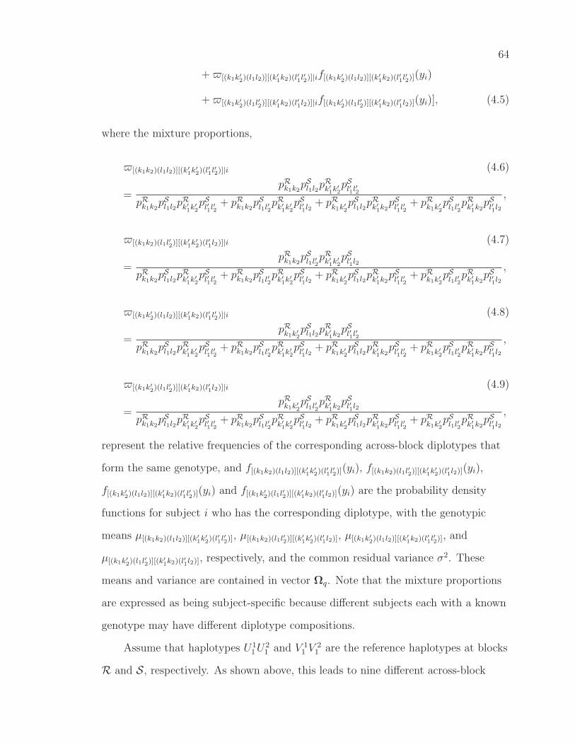
64
+[(k1k′2)(l1l2)][(k′
1k2)(l′1l′2)]|if[(k1k′2)(l1l2)][(k′
1k2)(l′1l′2)](yi)
+[(k1k′2)(l1l′2)][(k′
1k2)(l′1l2)]|if[(k1k′2)(l1l′2)][(k′
1k2)(l′1l2)](yi)], (4.5)
where the mixture proportions,
[(k1k2)(l1l2)][(k′1k′
2)(l′1l′2)]|i (4.6)
=pRk1k2
pSl1l2pRk′
1k′2pSl′1l′2
pRk1k2pSl1l2
pRk′1k′
2pSl′1l′2
+ pRk1k2pSl1l′2
pRk′1k′
2pSl′1l2
+ pRk1k′2pSl1l2
pRk′1k2pSl′1l′2
+ pRk1k′2pSl1l′2
pRk′1k2pSl′1l2
,
[(k1k2)(l1l′2)][(k′1k′
2)(l′1l2)]|i (4.7)
=pRk1k2
pSl1l′2pRk′
1k′2pSl′1l2
pRk1k2pSl1l2
pRk′1k′
2pSl′1l′2
+ pRk1k2pSl1l′2
pRk′1k′
2pSl′1l2
+ pRk1k′2pSl1l2
pRk′1k2pSl′1l′2
+ pRk1k′2pSl1l′2
pRk′1k2pSl′1l2
,
[(k1k′2)(l1l2)][(k′
1k2)(l′1l′2)]|i (4.8)
=pRk1k′
2pSl1l2
pRk′1k2pSl′1l′2
pRk1k2pSl1l2
pRk′1k′
2pSl′1l′2
+ pRk1k2pSl1l′2
pRk′1k′
2pSl′1l2
+ pRk1k′2pSl1l2
pRk′1k2pSl′1l′2
+ pRk1k′2pSl1l′2
pRk′1k2pSl′1l2
,
[(k1k′2)(l1l′2)][(k′
1k2)(l′1l2)]|i (4.9)
=pRk1k′
2pSl1l′2
pRk′1k2pSl′1l2
pRk1k2pSl1l2
pRk′1k′
2pSl′1l′2
+ pRk1k2pSl1l′2
pRk′1k′
2pSl′1l2
+ pRk1k′2pSl1l2
pRk′1k2pSl′1l′2
+ pRk1k′2pSl1l′2
pRk′1k2pSl′1l2
,
represent the relative frequencies of the corresponding across-block diplotypes that
form the same genotype, and f[(k1k2)(l1l2)][(k′1k′
2)(l′1l′2)](yi), f[(k1k2)(l1l′2)][(k′1k′
2)(l′1l2)](yi),
f[(k1k′2)(l1l2)][(k′
1k2)(l′1l′2)](yi) and f[(k1k′2)(l1l′2)][(k′
1k2)(l′1l2)](yi) are the probability density
functions for subject i who has the corresponding diplotype, with the genotypic
means µ[(k1k2)(l1l2)][(k′1k′
2)(l′1l′2)], µ[(k1k2)(l1l′2)][(k′1k′
2)(l′1l2)], µ[(k1k′2)(l1l2)][(k′
1k2)(l′1l′2)], and
µ[(k1k′2)(l1l′2)][(k′
1k2)(l′1l2)], respectively, and the common residual variance σ2. These
means and variance are contained in vector Ωq. Note that the mixture proportions
are expressed as being subject-specific because different subjects each with a known
genotype may have different diplotype compositions.
Assume that haplotypes U11U
21 and V 1
1 V21 are the reference haplotypes at blocks
R and S, respectively. As shown above, this leads to nine different across-block

65
composite genotypes. equation (4.1) provides the structure of an arbitrary across-
block composite genotype formed by the reference and non-reference haplotypes.
The log-likelihood function described by equation (4.5) can now be expressed, in
specific forms, as
logL(Ωp,Ωq|y,n) = (4.10)n(11/11)(11/11)∑
i=1
log fAABB(yi) +
n(11/11)(•)∑
i=1
log fAABB(yi) +
n(11/11)(••)∑
i=1
log fAABB(yi)
+
n(11/11)(12/12)∑
i=1
log[SfAABB(yi) + (1 −S)fAABB(yi)]
+
n(•)(11/11)∑
i=1
log fAABB(yi) +
n(•)(•)∑
i=1
log fAABB(yi) +
n(•)(••)∑
i=1
log fAABB(yi)
+
n(•)(12/12)∑
i=1
log[SfAABB(yi) + (1 −S)fAABB(yi)]
+
n(••)(11/11)∑
i=1
log fAABB(yi) +
n(••)(•)∑
i=1
log fAABB(yi) +
n(••)(••)∑
i=1
log fAABB(yi)
+
n(••)(12/12)∑
i=1
log[SfAABB(yi) + (1 −S)fAABB(yi)]
+
n(12/12)(11/11)∑
i=1
log[RfAABB(yi) + (1 −R)fAABB(yi)]
+
n(12/12)(•)∑
i=1
log[RfAABB(yi) + (1 −R)fAABB(yi)]
+
n(12/12)(••)∑
i=1
log[RfAABB(yi) + (1 −R)fAABB(yi)]
+
n(12/12)(12/12)∑
i=1
log[[(11)(11)][(22)(22)]fAABB(yi) +[(11)(12)][(22)(21)]fAABB(yi)
+[(12)(11)][(21)(22)]fAABB(yi) +[(12)(12)][(21)(21)]fAABB(yi)],
where
n(11/11)(•) = n(11/11)(11/12) + n(11/11)(12/11),

66
n(11/11)(••) = n(11/11)(11/22) + n(11/11)(12/22) + n(11/11)(22/11) + n(11/11)(22/12)
+n(11/11)(22/22),
n(•)(11/11) = n(11/12)(11/11) + n(12/11)(11/11),
n(••)(11/11) = n(11/22)(11/11) + n(12/22)(11/11) + n(22/11)(11/11) + n(22/12)(11/11)
+n(22/22)(11/11),
n(•)(•) = n(11/12)(11/12) + n(11/12)(12/11) + n(12/11)(11/12) + n(12/11)(12/11),
n(•)(••) = n(11/12)(11/22) + n(11/12)(12/22) + n(11/12)(22/11) + n(11/12)(22/12) +
n(11/12)(22/22) + n(12/11)(11/22) + n(12/11)(12/22) + n(12/11)(22/11) +
n(12/11)(22/12) + n(12/11)(22/22),
n(••)(•) = n(11/22)(11/12) + n(12/22)(11/12) + n(22/11)(11/12) + n(22/12)(11/12) +
n(22/22)(11/12) + n(11/22)(12/11) + n(12/22)(12/11) + n(22/11)(12/11) +
n(22/12)(12/11) + n(22/22)(12/11),
n(••)(••) = n(11/22)(11/22) + n(11/22)(12/22) + n(11/22)(22/11) + n(11/22)(22/12) +
n(11/22)(22/22) + n(12/22)(11/22) + n(12/22)(12/22) + n(12/22)(22/11) +
n(12/22)(22/12) + n(12/22)(22/22) + n(22/11)(11/22) + n(22/11)(12/22) +
n(22/11)(22/11) + n(22/11)(22/12) + n(22/11)(22/22) + n(22/12)(11/22) +
n(22/12)(12/22) + n(22/12)(22/11) + n(22/12)(22/12) + n(22/12)(22/22) +
n(22/22)(11/22) + n(22/22)(12/22) + n(22/22)(22/11) + n(22/22)(22/12) +
n(22/22)(22/22),
n(•)(12/12) = n(11/12)(12/12) + n(12/11)(12/12),
n(12/12)(•) = n(12/12)(11/12) + n(12/12)(12/11),
n(••)(12/12) = n(11/22)(12/12) + n(12/22)(12/12) + n(22/11)(12/12) + n(22/12)(12/12) +
n(22/22)(12/12),

67
n(12/12)(••) = n(12/12)(11/22) + n(12/12)(12/22) + n(12/12)(22/11) + n(12/12)(22/12) +
n(12/12)(22/22),
R =pR11p
R22
pR11pR22 + pR12p
R21
, (4.11)
S =pS11p
S22
pS11pS22 + pS12p
S21
, (4.12)
and [(11)(11)][(22)(22)], [(11)(12)][(22)(21)], [(12)(11)][(21)(22)] and [(12)(12)][(21)(21)] are the
mixture proportions for the complete heterozygous genotype at all the four SNPs
from two blocks and can be expressed by Equations (4.6) – (4.9). Different from
Equations (4.6) – (4.9), these expressions ignore i because all subjects with the
complete heterozygous genotype have the same diplotype composition.
4.2.4 An Integrative EM Algorithm
I derived a closed-form solution for estimating the unknown parameters with
the EM algorithm. The estimates of haplotype frequencies are based on the log-
likelihood function of equation (4.4), whereas the estimates of diplotype genotypic
means and residual variance are based on the log-likelihood function of equation
(4.5). These two different types of parameters can be estimated using an integrative
EM algorithm (APPENDIX B).
Haplotype frequencies can be expressed as a function of allelic frequencies and
LD. For a two-SNP haplotype within block R, I have
pRk1k2= p
R(1)k1
pR(2)k2
+ (−1)k1+k2DR, (4.13)
where DR is the linkage disequilibrium between the two SNPs at block R. Thus,
once haplotype frequencies are estimated, I can estimate allelic frequencies and LD
by solving equation (4.13). Similar calculations are also done for block S. After
across-block composite genotypic values are estimated, I can estimate the additive,
dominant and epistatic effects between two blocks using equation (4.2). The

68
standard errors of the MLEs of the population and quantitative genetic parameters
can be estimated on the basis of Louis’ (1982) observed information matrix.
4.3 Hypothesis Tests
Two major hypotheses can be made in the following sequence: (1) the associ-
ation between different SNPs within each block by testing their linkage disequilib-
rium (LD), and (2) the significance of an assumed reference haplotype for its effect
on the disease outcome. The LD between two given SNPs within block R can be
tested using the following hypotheses:
H0 : DR = 0
H1 : DR 6= 0
(4.14)
The log-likelihood ratio test statistic for the significance of LD is calculated by
comparing the likelihood values under the H1 (full model) and H0 (reduced model)
using
LRR = −2[logL(pR(1)k1
, pR(2)k2
, DR = 0, Ωq|n) − logL(Ωp, Ωq|n)] (4.15)
where the tilde and hat denote the MLEs of unknown parameters under H0 and H1,
respectively. The LRR is considered to asymptotically follow a χ2 distribution with
one degree of freedom. The MLEs of allelic frequencies under H0 can be estimated
using the EM algorithm described above, but with the constraint pR11pR22 = pR12p
R21. A
similar test can be made for block S.
Diplotype or haplotype effects on a complex disease can be tested using the
null and alternative hypotheses expressed as
H0 : µjRjS = µ
H1 : at least one equality in H0 does not hold
(4.16)
The log-likelihood ratio test statistic (LR) under these two hypotheses can be
similarly calculated. The LR may asymptotically follow a χ2 distribution with

69
eight degree of freedom. However, the approximation of a χ2 distribution may be
inappropriate when some regularity conditions, such as normal and uncorrelated
residuals, are violated. The permutation test approach proposed by Churchill and
Doerge (1994), which does not rely upon the distribution of the LR, may be used to
determine the critical threshold for determining the existence of a QTL.
Different genetic effects, such as the additive (αR and αS), dominant (βR and
βS) and additive × additive (I), additive × dominant (J), dominant × additive
(K) and dominant × dominant effects (L) between blocks R and S can also be
tested individually. The critical thresholds for these individual effects can be
determined on the basis of simulation studies.
4.4 Results
I use a real example from an obesity study to demonstrate the power and
usefulness of this model. Numerous genes have been investigated as potential
obesity-susceptibility genes (Mason et al. 1999; Chagnon et al. 2003). The β1AR
and β2AR genes are two such examples (Green et al. 1995; Large et al. 1997) in
each of which there are several polymorphisms common in the population. Two
common polymorphisms are identified at codons 49 and 389 for the β1AR gene
on chromosome 10 and at codons 16 and 27 for the β2AR gene on chromosome 5,
respectively. The polymorphisms in each of these two receptor genes are in linkage
disequilibrium, which suggests the importance of taking into account haplotypes,
rather than a single polymorphism, when defining biologic function. This study
attempts to detect haplotype variants within these candidate genes which determine
human obesity traits.
To determine whether sequence variants at the two polymorphisms from one
gene interact with those from the other gene to affect obesity phenotypes, a group
of 163 men and women were investigated with ages from 32 to 86 years old with a
large variation in body fat mass. Each of these patients was determined for their

70
genotypes at codon 49 with two alleles, Ser49 (A) and Gly49 (G), and codon 389
with two alleles, Arg389 (C) and Gly389 (G), within the β1AR gene, as well as
at codon 16 with two alleles, Arg16 (A) and Gly16 (G), and codon 27 with two
alleles, Gln27 (C) and Glu27 (G), within the β2AR gene, and measured for body
mass index (BMI). Two SNPs from each gene theoretically form 81 across-gene
genotypes, but, because these two genes are independent, the frequencies of these
genotypes can be expressed as the product of the genotype frequencies from each
gene. The integrative EM algorithm based on the likelihood function (4.4) allows
for the estimates of four haplotype frequencies and the resulting allele frequencies
and linkage disequilibrium at each gene (Table 4-2). Highly significant LD was
detected between two SNPs for each gene (P < 0.001). Small sampling errors for
the estimates of each population genetic parameter indicated that the estimates are
highly precise.
By assuming that one haplotype is different from the rest of haplotypes at
each gene, this model can detect the reference haplotypes that display significant
main and interaction effects on the BMI trait. Using haplotypes AC, AG, GC
and GG as a reference haplotype at the β1AR gene, respectively, in conjunction
with a reference haplotype selected from AC, AG, GC or GG at the β2AR gene,
I calculated the corresponding log-likelihood-ratio (LR) test statistics (0.36 –
17.90) using equation (4.10) (Table 4-2). Based on the critical threshold value of
15.05 at the 5% significance level determined from 1000 permutation tests, the two
maximal LR values, 15.1 and 17.9 for across-gene reference haplotypes (GG)(GC)
and (GC)(GC), respectively, are thought to trigger significant haplotype effects on
BMI. However, because these two reference haplotypes form different numbers of
composite genotypes, with all nine for (GG)(GC) and eight for (GC)(GC) (Table
4-2), an optimal reference-haplotype combination should be selected on the basis
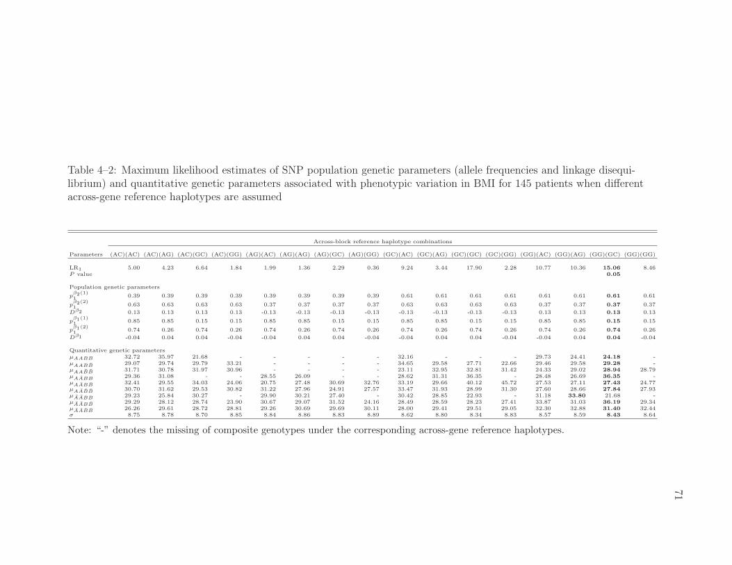
71
Table 4–2: Maximum likelihood estimates of SNP population genetic parameters (allele frequencies and linkage disequi-librium) and quantitative genetic parameters associated with phenotypic variation in BMI for 145 patients when differentacross-gene reference haplotypes are assumed
Across-block reference haplotype combinations
Parameters (AC)(AC) (AC)(AG) (AC)(GC) (AC)(GG) (AG)(AC) (AG)(AG) (AG)(GC) (AG)(GG) (GC)(AC) (GC)(AG) (GC)(GC) (GC)(GG) (GG)(AC) (GG)(AG) (GG)(GC) (GG)(GG)
LR1 5.00 4.23 6.64 1.84 1.99 1.36 2.29 0.36 9.24 3.44 17.90 2.28 10.77 10.36 15.06 8.46P value 0.05
Population genetic parameters
pβ2(1)1 0.39 0.39 0.39 0.39 0.39 0.39 0.39 0.39 0.61 0.61 0.61 0.61 0.61 0.61 0.61 0.61
pβ2(2)1 0.63 0.63 0.63 0.63 0.37 0.37 0.37 0.37 0.63 0.63 0.63 0.63 0.37 0.37 0.37 0.37
Dβ2 0.13 0.13 0.13 0.13 -0.13 -0.13 -0.13 -0.13 -0.13 -0.13 -0.13 -0.13 0.13 0.13 0.13 0.13
pβ1(1)1 0.85 0.85 0.15 0.15 0.85 0.85 0.15 0.15 0.85 0.85 0.15 0.15 0.85 0.85 0.15 0.15
pβ1(2)1 0.74 0.26 0.74 0.26 0.74 0.26 0.74 0.26 0.74 0.26 0.74 0.26 0.74 0.26 0.74 0.26
Dβ1 -0.04 0.04 0.04 -0.04 -0.04 0.04 0.04 -0.04 -0.04 0.04 0.04 -0.04 -0.04 0.04 0.04 -0.04
Quantitative genetic parametersµAABB 32.72 35.97 21.68 - - - - - 32.16 - - - 29.73 24.41 24.18 -µAABB 29.07 29.74 29.79 33.21 - - - - 34.65 29.58 27.71 22.66 29.46 29.58 29.28 -µAABB 31.71 30.78 31.97 30.96 - - - - 23.11 32.95 32.81 31.42 24.33 29.02 28.94 28.79µAABB 29.36 31.08 - - 28.55 26.09 - - 28.62 31.31 36.35 - 28.48 26.69 36.35 -µAABB 32.41 29.55 34.03 24.06 20.75 27.48 30.69 32.76 33.19 29.66 40.12 45.72 27.53 27.11 27.43 24.77µAABB 30.70 31.62 29.53 30.82 31.22 27.96 24.91 27.57 33.47 31.93 28.99 31.30 27.60 28.66 27.84 27.93µAABB 29.23 25.84 30.27 - 29.90 30.21 27.40 - 30.42 28.85 22.93 - 31.18 33.80 21.68 -µAABB 29.29 28.12 28.74 23.90 30.67 29.07 31.52 24.16 28.49 28.59 28.23 27.41 33.87 31.03 36.19 29.34µAABB 26.26 29.61 28.72 28.81 29.26 30.69 29.69 30.11 28.00 29.41 29.51 29.05 32.30 32.88 31.40 32.44σ 8.75 8.78 8.70 8.85 8.84 8.86 8.83 8.89 8.62 8.80 8.34 8.83 8.57 8.59 8.43 8.64
Note: “-” denotes the missing of composite genotypes under the corresponding across-gene reference haplotypes.

72
of the AIC criterion. I found that across-gene reference haplotype (GC)(GC) is the
best for explaining the BMI data in this example.
The missing of one composite genotype generated by across-gene reference
haplotype (GC)(GC) prevents the estimation of all the additive, dominant and
epistatic effects using equation (4.2) because of inadequate degrees of freedom. As
an example, I used across-gene reference haplotype (GG)(GC) to demonstrate how
each of these genetic effects is tested. It is found that the additive and dominant
effects exerted by (GG)(GC) are not significant (data not shown). Of the four
kinds of epistasis between the two genes, only dominant × dominant genetic effect
is significant at the 5% significance level. This type of epistasis reduces, by about
20%, the BMI of the patient who carries diplotypes [GG][GG] at the β2AR gene
and [GC][GC] at the β1AR gene, compared to the other across-gene diplotypes.
I estimate the standard errors of the MLEs of the population and quantitative
genetic parameters based on Louis’ (1982) observed information matrix, suggesting
that all MLEs have reasonable estimation precision although the estimates of
quantitative genetic parameters are not as precise as those of population genetic
parameters due to a small sample size used.
4.5 Discussion
For any two unrelated people, about 99.9% of their DNA sequences are
detected to be the same. It is the remaining 0.1% that contains the genetic variants
that influence how people differ in their risk of disease or their response to drugs.
Discovering concrete DNA sequence variants that contribute to common disease risk
offers one of the best opportunities for understanding the complex causes of disease
in humans. The recent development of a haplotype map of the human genome, the
HapMap, by the International HapMap Consortium (2003) provides a key resource
to describe the common patterns of human DNA sequence variation and find genes
that affect health, disease, and responses to drugs and environmental factors.

73
I have recently developed a series of statistical models that can detect specific
DNA sequence variants for complex diseases (Liu et al. 2004) or drug response (Lin
et al. 2005) with the aids of the information provided by the HapMap. Different
from quantitative trait loci (QTL) defined as putative chromosomal segments, DNA
sequence variants detected from my models are shown at the individual nucleotide
level, which are therefore called quantitative trait nucleotides (QTN). Although the
models for QTN mapping have been studied by theoretical simulations and vali-
dated with real-world data, their applications may still be limited because of their
underlying assumption that genes operate individually. For most common diseases,
such as diabetes, cancer, obesity, stroke, heart disease, depression, and asthma,
however, it is likely that a suite of genes and environmental factors are involved to
form a complicated web of interactions (Segre et al. 2005). Interactions between
different genes (i.e., epistasis) or between genes and environmental factors are
thought to be evolutionary forces to maintain genetic variation and buffer against
environmental or developmental perturbations (Moore 2005). In this chapter, I
extend my earlier statistical models to perform a genome-wide scan for sequence-
sequence interactions as a fundamental component of genetic network for disease
susceptibility. Beyond traditional epitstatic models based on locus cosegregations
(Lynch and Walsh 1998), this model allows for the direction characterization of spe-
cific DNA sequence interactions on the SNP-constructed HapMap. As an example,
I have used the data from an obesity research project to validate the implications
of my interactive models. Specific DNA sequences from two different candidate
genes, β1AR and β2AR, have been identified to affect human obesity traits in an
interactive manner.
For clarification, my presented the idea for sequencing a complex trait with
an interaction model based on two-DNA sequences from each haplotype block.
It is likely that the two-SNP model is too simple to characterize genetic variants

74
for quantitative variation. With the foundation for the two-SNP sequencing
model, I can readily extend this model to include an arbitrary number of SNPs
whose sequences are associated with the phenotypic variation. In the multi-SNP
sequencing model, I face many haplotypes and haplotype pairs. An AIC- or BIC-
based model selection strategy (Burnham and Andersson 1998) has been framed
to determine the haplotype that is most distinct from the rest of haplotypes in
explaining quantitative variation. However, in practice, a simultaneously analysis
of too many SNPs will encounter considerable computationally load and, also, may
not be necessary for the explanation of disease variation. The determination of a
maximal number of SNPs for sequencing mapping of QTN should be integrated
with computational algorithms for haplotype block modelling (Kimmel and Shamir
2005).
One of the most important statistical issues for QTN mapping is the derivation
of an effective approach to handle missing composite genotypes. For some reference
haplotypes, one or more composite genotypes are missing due to a low frequency of
their occurrences although their effects may exist. The missing of these composite
genotypes prevents the full estimates of the genetic effects. Given that these
composite genotypes are not missing at random, pattern mixture models developed
for treating non-randomly missing data (Little 1993, 1994) can be used to estimate
the genotypic values of missing composite genotypes. Thus, after the idea behind
the pattern mixture models is incorporated into the sequence mapping of QTN, I
are closer to provide better estimates of sequence action and interaction effects on
complex diseases.
CHAPTER 5MODEL FOR DETECTING SEQUENCE-SEQUENCE INTERACTIONS FOR
DRUG RESPONSE
5.1 Introduction
The increasing number of genetic studies for complex traits and biological
processes in humans requires more advanced techniques of statistical analysis
(Lynch and Walsh 1998). This is due to two reasons. First, genes interact in a
complex network to determine a final phenotype. It is very often that a complex
trait is characterized by a number of non-Mendelian, environmentally sensitive
genes, of which some act additively, whereas many others are operational in a
multiplicative or compensatory way (Frankel and Schork 1996; Moore 2003). Many
current statistical techniques used in genetic research assume the additive control
of genes, aimed to facilitate data analysis and modelling, which certainly provide
misleading results when genetic interactions or epistasis actually occur.
Second, almost every phenotypic trait can be partitioned into its multiple
continuous developmental components on a time scale. To better study the genetic
architecture of these traits, I need measure the traits at a multitude of discrete time
points. A different but statistically similar example of these so-called time-series
traits is drug response, a field that gained much attention due to the possible
clinical applications, ranging from individualized therapy to new drug development
(Arranz et al. 2002). Recent studies have suggested that a variable number of
polymorphisms in various genes are supposedly involved in modulating the response
and/or side effects to drugs (Serretti and Artioli 2003).
The motivation of this chapter is to develop a statistical model for detecting
epistatic interactions that control drug response. This new model is constructed
75
76
through combining two recent developments in genetic mapping. A traditional
mapping strategy is based on the cosegregation of genotyped markers and quan-
titative trait loci (QTL) that are bracketed by the markers (Lander and Botstein
1989). QTL for a complex trait identified from this strategy presents a hypothesized
chromosomal segment whose DNA sequence is unknown. The second strategy,
recently developed by Liu et al. (2004) and Lin et al. (2005), can identify specific
DNA sequence variants that affect a complex trait. This strategy, that relies on the
recent advent of high-throughout single nucleotide polymorphism (SNP) technolo-
gies, allows for the genomewide scan of causal DNA sequences, called quantitative
trait nucleotides (QTN). Lin et al. (2005) have developed a conceptual framework
for detecting interaction effects between different QTN for a complex trait.
Considering the dynamic feature of many complex traits, a series of statistical
models, called functional mapping, have been recently developed to characterize
QTL that contribute to genetic variation for longitudinal traits (Ma et al. 2002; Wu
et al. 2004a, 2004b, 2004c). Functional mapping capitalizes on the mathematical
functions that describe biological processes and embeds them within the context
of genetic mapping theory. By estimating the mathematical parameters that
determine the patterns of longitudinal trajectories, functional mapping has proven
efficient and effective for unveiling the genetic architecture of complex traits. In this
chapter, I incorporate the idea of QTN mapping with functional mapping to detect
epistatic interactions between different DNA sequence variants that encode drug
response. I also perform simulation studies to examine the statistical properties of
this model. A real example was used to validate the usefulness of this model.
5.2 Theory
5.2.1 The Normal Mixture Model
Approaches for QTL and QTN mapping are statistically similar in the con-
ceptual formation of a mixture model. For QTL mapping, each observation must

77
arise from one of multiple QTL genotypes, although the QTL genotype for this
individual is unknown (Lander and Botstein 1989). The normal mixture model is
constructed to contain the possible impact of these QTL genotypes each of which
is assumed to follow a normal distribution. As shown in Liu et al. (2004), QTN
mapping is also based on a normal mixture model but in which the phenotypic
value of an individual that is heterozygous for two or more SNPs is thought to arise
one of multiple diplotypes constructed by set of SNPs.
Differences among different diplotypes can be assumed to result from the
composition of different haplotypes. Liu et al. (2004) defined the haplotype
that is different from the rest of haplotypes as reference haplotype. Those rest of
haplotypes are thus defined as non-reference haplotype. Consider a QTN, R, that
is composed of a set of SNPs. Let A and A be the reference and non-reference
haplotypes for this QTN, respectively, which thus form three different composite
genotypes, AA, AA and AA. In the mixture model, longitudinal observations for
each composite genotype, j, are characterized by a different multivariate normal
distribution with mean vector uj and covariance matrix Σ.
For QTN mapping, only diplotypes that are heterozygous for two or more
SNPs contain different composite genotypes because these diplotypes are not
consistent with their phenotypically observable genotypes. Therefore, the mixture
model is formulated only for those diplotypes.
5.2.2 Epistatic Effects
I developed an interactive model aimed to detect sequence-sequence epistasis.
Let B and B be the reference and non-reference haplotypes at a second QTN, B,
respectively. The two QTN, A and B, generate nine different composite genotypes
expressed as AABB, AABB, AABB, AABB, AABB, AABB, AABB, AABB
and AABB. Traditional quantitative genetic theories can be used to model the
genetic effects of the composite genotypes (Lynch and Walsh 1998). The genotypic
78
vector (ujRjS ) of a joint composite genotype at the two haplotype blocks can be
decomposed into nine different components as follows:
ujRjS = u Overall mean (5.1)
+ (jR − 1)aR + (jS − 1)aS Additive effects
+ [1 − (jR − 1)2]bR + [1 − (jS − 1)2]bS Dominant effects
+ (jR − 1)(jS − 1)i Additive × additive effect
+ (jR − 1)[1 − (jS − 1)2]j Additive × dominant effect
+ [1 − (jR − 1)2](jS − 1)k Dominant × additive effect
+ [1 − (jR − 1)2][1 − (jS − 1)2]l Dominant × dominant effect,
where
jR, jS =
2 for AA or BB
1 for AA or BB
0 for AA or BB
stand for the composite genotypes at blocks R and S, respectively, a. and b. are
the additive and dominant effect vectors at the corresponding block, respectively,
and i, j, k and l are the additive × additive, additive × dominant, dominant ×
additive and dominant × dominant epistatic effect vectors between the two QTN,
respectively.
If the maximum likelihood estimates (MLEs) of the genotypic value vectors at
the left side of equation (5.1) can be observed, I can solve the vectors for the overall
mean, additive, dominant and four kinds of epistatic effects between two QTN by
u =1
4(uAABB + uAABB + uAABB + uAABB)
aR =1
4(uAABB − uAABB + uAABB − uAABB)
aS =1
4(uAABB − uAABB − uAABB + uAABB)

79
bR =1
4(2uAABB − uAABB − uAABB − uAABB − uAABB + 2uAABB)
bS =1
4(2uAABB − uAABB − uAABB − uAABB − uAABB + 2uAABB)
i =1
4(uAABB − uAABB − uAABB + uAABB)
j =1
4(2uAABB − uAABB − 2uAABB + uAABB − uAABB + uAABB)
k =1
4(2uAABB − 2uAABB + uAABB + uAABB − uAABB − uAABB)
l =1
4(4uAABB + uAABB + uAABB + uAABB + uAABB − 2uAABB
−2uAABB − 2uAABB − 2uAABB) (5.2)
5.2.3 Likelihood Functions
The mixture model used to map QTN includes the proportions of each mixture
component and the probability distribution functions of phenotypic observations
given that component. The mixture proportions are the relative frequencies of
those diplotypes that are phenotypically the same and they can be expressed as
a function of haploid frequencies. In this chapter, two QTN are assumed to be
independent, which means that their joint haplotype frequencies are the products of
two haplotype frequencies each from a QTN.
Suppose there are R and S SNPs for QTN R and S, respectively. The two
alleles, 1 and 2, at each of these SNPs are symbolized by k1, . . . , kR and l1, . . . , lR,
respectively. A haplotype frequency is denoted by pRk1k2···kRfor QTN R and pSl1l2···lS
for QTN S. As stated above, across-QTN haplotype frequencies can be calculated
as the product of the corresponding haplotype frequencies from a different QTN,
expressed as
p(k1k2···kR)(l1l2···lS) = pRk1k2···kRpSl1l2···lS
, (5.3)
where the parentheses are used to separate two different QTN for a given across-
QTN haplotype. With these across-QTN haplotype frequencies, expected across-
80
QTN diplotype frequencies and across-QTN genotype frequencies can be calculated,
respectively, under Hardy-Weinberg equilibrium (Lynch and Walsh 1998).
With across-QTN diplotype and genotype frequencies, the likelihood function
based on across-QTN genotype observations, n = n(k1k′1/k2k′
2/···/kRk′
R)(l1l′1/l2l′2/···/lS l′S),
can be constructed. I simplify the presentation of the model by assuming two SNPs
for each QTN. In Table 5-1, all possible genotypes and diplotypes are given as
well as their frequencies at two SNPs genotyped from QTN R. Each diplotype
is composed of two haplotypes, one from the mother and the other from the
father. The diplotype frequencies can be expressed in terms of the haplotype
frequencies. The same genotype may contain two different diplotypes, depending
on its heterozygosity. Table 5-1 also provides the relative frequencies with which a
genotype carries a particular haplotype. Such relative frequencies will be useful for
partitioning observed genotypes into underlying diplotypes in the construction of
likelihood function based on the phneotype.
Let Ωp = (pRk1k2, pSl1l2
) be the population genetic parameters to be estimated
for QTN R and S. Lin et al.(2005) formulated a log-likelihood function of these
unknown haplotype frequencies given observed genotypes (n) in a multinomial
form. They also provided a series of closed-form solution for the EM algorithm to
estimate these haplotype frequencies. To save space, a detailed procedure for this
estimation process is not given.
While traditional models assume the association between the genotype and
drug response (Gong et al. 2004), this model can estimate the effects of different
diplotypes on the pharmacodynamic response of drugs. A particular four-SNP
genotype from two QTN, expressed as (k1k′1/k2k
′2)(l1l
′1/l2l
′2), can be partitioned
into four possible diplotypes, [(k1k2)(l1l2)][(k′1k
′2)(l
′1l
′2)], [(k1k2)(l1l
′2)][(k
′1k
′2)(l
′1l2)],
[(k1k′2)(l1l2)][(k
′1k2)(l
′1l
′2)] and [(k1k
′2)(l1l
′2)] [(k′1k2)(l
′1l2)]. Let Ωq be quantitative
genetic parameters that specify the mean vectors of different diplotypes and the

81
Table 5–1: Possible diplotypes and their frequenecies for each of nine genotypes at two SNPs within a QTN, haplotype com-position frequencies for each genotype and genotypic value vectors of composite genotypes
Relative diplotype Haplotype composition Composite GenotypicGenotype Diplotype Diplotype frequency freq. within genotypes [11] [12] [21] [22] genotype mean vector
11/11 [11][11] P[11][11] = p211 1 1 0 0 0 AA u2·
11/12 [11][12] P[11][12] = 2p11p12 1 12
12 0 0 AA u1·
11/22 [12][12] P[12][12] = p212 1 0 1 0 0 AA u0·
12/11 [11][21] P[11][21] = 2p11p21 1 12 0 1
2 0 AA u1·
12/12
[11][22]
[12][21]
P[11][22] = 2p11p22
P[12][21] = 2p12p21
π
1 − π12π 1
2(1 − π) 12(1 − π) 1
2π
AA
AA
u1·
u0·
12/22 [12][22] P[12][22] = 2p12p22 1 0 12 0 1
2 AA u0·
22/11 [21][21] P[21][21] = p221 1 0 0 1 0 AA u0·
22/12 [21][22] P[21][22] = 2p21p22 1 0 0 12
12 AA u0·
22/22 [22][22] P[22][22] = p222 1 0 0 0 1 AA u0·
Two alleles for each of the two SNPs are denoted as 1 and 2, respectively. Genotypes at different SNPs are separated by a slash.Diplotypes are the combination of two bracketed maternally and paternally derived haplotypes. By assuming that haplotype [11] is thereference haplotype, composite genotypes are accordingly defined and their genotypic mean vectors are given. π = p11p22
p11p22+p12p21where
p11, p12, p21 and p22 are the haplotype frequencies of [11], [12], [21], and [22], respectively. ujR·=
∑jS=2jS=0 ujRjS .

82
residual covariance matrix. The likelihood of unknown population (Ωp) and
quantitative genetic parameters (Ωq) given a drug response measured at C dosage
levels, y = y(1), . . . , y(C), and SNP genotype observations, n, is constructed as
logL(Ωp,Ωq|y,n) =n∑
i=1
log[[(k1k2)(l1l2)][(k′1k′
2)(l′1l′2)]|if[(k1k2)(l1l2)][(k′1k′
2)(l′1l′2)](yi)
+ [(k1k2)(l1l′2)][(k′1k′
2)(l′1l2)]|if[(k1k2)(l1l′2)][(k′1k′
2)(l′1l2)](yi)
+ [(k1k′2)(l1l2)][(k′
1k2)(l′1l′2)]|if[(k1k2)(l′1l2)][(k′1k′
2)(l′1l2)](yi)
+ [(k1k′2)(l1l′2)][(k′
1k2)(l1l′2)]|if[(k1k′2)(l1l′2)][(k′
1k2)(l′1l2)](yi)],
(5.4)
where the mixture proportions,
[(k1k2)(l1l2)][(k′1k′
2)(l′1l′2)]|i (5.5)
=pRk1k2
pSl1l2pRk′
1k′2pSl′1l′2
pRk1k2pSl1l2
pRk′1k′
2pSl′1l′2
+ pRk1k2pSl1l′2
pRk′1k′
2pSl′1l2
+ pRk1k′2pSl1l2
pRk′1k2pSl′1l′2
+ pRk1k′2pSl1l′2
pRk′1k2pSl′1l2
,
[(k1k2)(l1l′2)][(k′1k′
2)(l′1l2)]|i (5.6)
=pRk1k2
pSl1l′2pRk′
1k′2pSl′1l2
pRk1k2pSl1l2
pRk′1k′
2pSl′1l′2
+ pRk1k2pSl1l′2
pRk′1k′
2pSl′1l2
+ pRk1k′2pSl1l2
pRk′1k2pSl′1l′2
+ pRk1k′2pSl1l′2
pRk′1k2pSl′1l2
,
[(k1k′2)(l1l2)][(k′
1k2)(l′1l′2)]|i (5.7)
=pRk1k′
2pSl1l2
pRk′1k2pSl′1l′2
pRk1k2pSl1l2
pRk′1k′
2pSl′1l′2
+ pRk1k2pSl1l′2
pRk′1k′
2pSl′1l2
+ pRk1k′2pSl1l2
pRk′1k2pSl′1l′2
+ pRk1k′2pSl1l′2
pRk′1k2pSl′1l2
,
[(k1k′2)(l1l′2)][(k′
1k2)(l′1l2)]|i (5.8)
=pRk1k′
2pSl1l′2
pRk′1k2pSl′1l2
pRk1k2pSl1l2
pRk′1k′
2pSl′1l′2
+ pRk1k2pSl1l′2
pRk′1k′
2pSl′1l2
+ pRk1k′2pSl1l2
pRk′1k2pSl′1l′2
+ pRk1k′2pSl1l′2
pRk′1k2pSl′1l2
,
represent the relative frequencies of the corresponding across-block diplotypes that
form the same genotype, and f[(k1k2)(l1l2)][(k′1k′
2)(l′1l′2)](yi), f[(k1k2)(l1l′2)][(k′1k′
2)(l′1l2)](yi),
f[(k1k2)(l′1l2)][(k′1k′
2)(l′1l2)](yi) and f[(k1k′2)(l1l′2)][(k′
1k2)(l′1l2)](yi) are the probability density
functions for subject i who has the corresponding diplotype, with C-dimensional

83
genotypic value vectors u[(k1k2)(l1l2)][(k′1k′
2)(l′1l′2)], u[(k1k2)(l1l′2)][(k′1k′
2)(l′1l2)], u[(k1k2)(l′1l2)][(k′1k′
2)
(l′1l2)], and u[(k1k′2)(l1l′2)][(k′
1k2)(l′1l2)], respectively, and C × C common residual covariance
matrix Σ. Note that the mixture proportions are expressed as being subject-specific
because different subjects each with a known genotype may have different diplotype
compositions.
Assume that haplotypes 11 (denoted by A) and 12 (denoted B) are the
reference haplotypes at QTN R and S, respectively. As shown above, this leads
to nine different across-QTN composite genotypes. equation (5.1) provides the
structure of an arbitrary across-QTN composite genotype formed by the reference
and non-reference haplotypes. Table 5-1 tabulates the genotypic value vectors
for different composite genotypes. For a given composite genotype jRjS , I have a
multivariate normal distribution expressed as
fjRjS (yi;Ωq) =1
(2π)C/2|Σ|1/2exp
[−1
2(yi − ujRjS )Σ−1(yi − ujRjS )′
], (5.9)
with jR, jS = 2, 1, 0. At a particular concentration c, the relationship between the
observation and expected mean can be described by a regression model (Zhao et al.
2005),
yi(c) =2∑
jR=0
2∑
jS=0
ξijRjSujRjS (c) + ei(c), (5.10)
=2∑
jR=0
2∑
jS=0
ξijRjSujRjS (c)
+r∗∑
c′=1
2∑
jR=0
2∑
jS=0
φ(c, c− c′)[yi(c− c′) − ξijRjSµjRjS (c− c′)] + ǫi(c) (5.11)
where ξijRjS is the indicator variable denoted as 1 if a composite genotype jRjS
is considered for individual i and 0 otherwise; ei(c) is the residual error (i.e.,
the accumulative effect of polygenes and errors) that contains two components,
rth-order antedependent variance (Gabriel 1962; Nunez-Anton and Zimmerman

84
2000),∑r∗
t′=1
∑2jR=1
∑2jS=1 φ(c, c − c′)[yi(c − c′) − ξijRjSµjRjS (c − c′)], where r∗ =
min(r, c − 1) and φ(c, c − c′)’s are unrestricted antedependence parameters, and
independent normal random variable, ǫi(c), with mean zero and time-dependent
variance, σ2(c), termed innovation variance.
5.2.4 Modelling the Mean-covariance Structures
Traditional genetic mapping for multiple traits attempts to estimate each
element in the mean vector and the covariance matrix. This may not be efficient
and effective for two reasons. First, when dosage level C is high, an exponentially
increasing number of parameters need to be estimated. Second, this approach does
not consider biological principles underlying pharmacodynamic responses. The
mainstay of modelling drug response is the Hill, or sigmoid Emax, equation, which
postulates the following relationship between drug concentration (C) and drug effect
(E) (Giraldo 2003)
E = E0 +EmaxC
H
ECH50 + CH
, (5.12)
where E0 is the constant or baseline value for the drug response parameter, Emax is
the asymptotic (limiting) effect, EC50 is the drug concentration that results in 50%
of the maximal effect, and H is the slope parameter that determines the slope of the
concentration-response curve. The larger H, the steeper the linear phase of the the
log-concentration-effect curve. When the effect is a continuous variable, estimates
of Emax, EC50 and H are usually obtained by extended least squares or iteratively
reweighted least squares when there is sufficient data for analysis of individual
subjects. When sparse data are pooled from multiple patients, then a population
analysis is a better approach. Different from such a traditional treatment, I will
estimate these curve parameters separately for different composite genotypes.
The composite genotype-specific mean vectors in equation (5.9) will be
modelled by the Emax model, expressed as
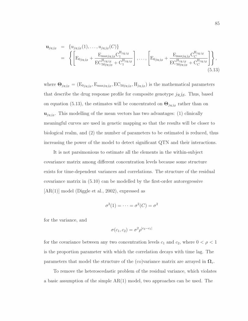
85
ujRjS = ujRjS (1), . . . , ujRjS (C)
=
[E0jRjS +
EmaxjRjSCHjRjS1
ECHjRjS50jRjS
+ CHjRjS1
], . . . ,
[E0jRjS +
EmaxjRjSCHjRjSC
ECHjRjS50jRjS
+ CHjRjSC
],
(5.13)
where ΘjRjS = (E0jRjS ,EmaxjRjS ,EC50jRjS ,HjRjS ) is the mathematical parameters
that describe the drug response profile for composite genotype jRjS . Thus, based
on equation (5.13), the estimates will be concentrated on ΘjRjS rather than on
ujRjS . This modelling of the mean vectors has two advantages: (1) clinically
meaningful curves are used in genetic mapping so that the results will be closer to
biological realm, and (2) the number of parameters to be estimated is reduced, thus
increasing the power of the model to detect significant QTN and their interactions.
It is not parsimonious to estimate all the elements in the within-subject
covariance matrix among different concentration levels because some structure
exists for time-dependent variances and correlations. The structure of the residual
covariance matrix in (5.10) can be modelled by the first-order autoregressive
[AR(1)] model (Diggle et al., 2002), expressed as
σ2(1) = · · · = σ2(C) = σ2
for the variance, and
σ(c1, c2) = σ2ρ|c2−c1|
for the covariance between any two concentration levels c1 and c2, where 0 < ρ < 1
is the proportion parameter with which the correlation decays with time lag. The
parameters that model the structure of the (co)variance matrix are arrayed in Ωv.
To remove the heteroscedastic problem of the residual variance, which violates
a basic assumption of the simple AR(1) model, two approaches can be used. The

86
first approach is to model the residual variance by a parametric function of time,
as originally proposed by Pletcher and Geyer (1999). But this approach needs to
implement additional parameters for characterizing the age-dependent change of the
variance. The second approach is to embed Carroll and Rupert’s (1984) transform-
both-sides (TBS) model into the growth-incorporated finite mixture model (Wu
et al. 2004b), which does not need any more parameters. Both empirical analyses
with real examples and computer simulations suggest that the TBS-based model
can increase the precision of parameter estimation and computational efficiency.
Furthermore, the TBS model preserves original biological means of the curve
parameters although statistical analyses are based on transformed data.
The TBS-based model displays the potential to relax the assumption of vari-
ance stationarity, but the covariance stationarity issue remains unsolved. Zhao et
al. (2005) used Zimmerman and Nunez-Anton’s (1997) structured antedependence
(SAD) model to approach the age-specific change of correlation in the analysis of
longitudinal traits based on (5.5). Using matrix notation, the error term in (5.4)
can be expressed as
e = Aǫ (5.14)
where e = [e(1), · · · , e(C)]′
, ǫ = [ǫ(1), · · · , ǫ(C)]′
and for the SAD(1) model
A =
1 0 0 0
φ1 1 0 0
.... . .
φC−11 φC−2
1 · · · φ1 1
(5.15)
The variance-covariance matrix of the longitudinal trait is then expressed as
Σ = AΣǫA′
, (5.16)

87
where Σǫ is the innovation variance-covariance matrix and is expressed as:
Σǫ =
σ2(1) 0 0 · · · 0
0 σ2(2) 0 · · · 0
......
.... . .
...
0 0 0 · · · σ2(C)
.
The closed forms for the inverse and determinant of matrix Σ help to estimate the
parameters, Ωv = (φ1, · · · , φr, σ2), that model the matrix. The vector ΘjRjS and Ωv
form the quantitative genetic parameters Ωq.
As a simplified example with the SAD(1) model, under the assumption that
innovation variance is constant across different time points, Jaffrezic et al. (2003)
derived the analytical forms for variance and covariance functions among time-
dependent measurements, expressed, respectively, as
σ2(c) =1 − φ2c
1 − φ2σ2, (5.17)
σ(c1, c2) = φc2−c11 − φ2c1
1 − φ2σ2, c2 ≥ c1, (5.18)
for equally spaced repeated measurements. It can be seen that although constant
innovation variances are assumed, the residual variance can change with dosage
level (Jaffrezic et al. 2003). Also, for the simplest SAD model, the correlation
function is non-stationary because the correlation does not depend only on the dose
interval c2 − c1 but also depends on the start and end points of the interval, c1 and
c2.
5.2.5 An Integrative EM-simplex Algorithm
I derived a closed-form solution for estimating the population genetic para-
meters Ωp with the EM algorithm (Lin et al. 2005). The Nelder-Mead simplex
algorithm, originally proposed by Nelder and Mead (1965), can be used to estimate
the quantitative genetic parameters Ωq = (ΘjRjS ,Ωv). It is a direct search method

88
for nonlinear unconstrained optimization. It attempts to minimize a scalar-valued
nonlinear function using only function values, without any derivative information
(explicit or implicit). The algorithm uses linear adjustment of the parameters until
some convergence criterion is met. Simulation studies have proven that simplex
algorithm converges to the same solution more rapidly than the EM algorithm in
the classical functional mapping.
Haplotype frequencies can be expressed as a function of allelic frequencies and
linkage disequilibria (LD). For a two-SNP haplotype for QTN R, I have
pRk1k2= p
R(1)k1
pR(2)k2
+ (−1)k1+k2DR, (5.19)
where DR is the linkage disequilibrium between the two SNPs at QTN R. Thus,
once haplotype frequencies are estimated, I can estimate allelic frequencies and LD
by solving equation (5.19). Similar calculations are also done for block S. After
across-QTN composite genotypic values are estimated, I can estimate the additive,
dominant and epistatic effects between two QTN using equation (5.2).
5.3 Hypothesis Tests
With my epistatic model, I can make a number of hypothesis tests regarding
the genetic control of overall drug response to a spectrum of dosages and other
clinically important events. Two major hypotheses can be made in the following
sequence: (1) the association between different SNPs within each QTN by testing
their linkage disequilibria (LD), and (2) the significance of an assumed across-QTN
reference haplotype for its effect on drug response. The LD between two given
SNPs within QTN R can be tested using the following hypotheses:
H0 : DR = 0
H1 : DR 6= 0
(5.20)
The log-likelihood ratio test statistic for the significance of LD is calculated by

89
comparing the likelihood values under the H1 (full model) and H0 (reduced model)
using
LRR = −2[logL(pRk1, pRk2
, DR = 0, Ωq|n) − logL(Ωp, Ωq|n)] (5.21)
where the tilde and hat denote the MLEs of unknown parameters under H0 and H1,
respectively. The LRR is considered to asymptotically follow a χ2 distribution with
one degree of freedom. The MLEs of allelic frequencies under H0 can be estimated
using the EM algorithm described above, but with the constraint pR11pR22 = pR12p
R21. A
similar test can be made for block S.
Diplotype or haplotype effects on a complex disease can be tested using the
null and alternative hypotheses expressed as
H0 : ΘjRjS = Θ (jR, jS = 2, 1, 0)
H1 : at least one equality in H0 does not hold
(5.22)
The log-likelihood ratio test statistic (LR) under these two hypotheses can be
similarly calculated. The LR may asymptotically follow a χ2 distribution with
36 degrees of freedom. However, the approximation of a χ2 distribution may be
inappropriate when some regularity conditions, such as normal and uncorrelated
residuals, are violated. The permutation test approach proposed by Churchill and
Doerge (1994), which does not rely upon the distribution of the LR, may be used to
determine the critical threshold for determining the existence of a QTL.
Different genetic effects, such as the additive (aR and aS), dominant (bR and
bS) and additive × additive (i), additive × dominant (j), dominant × additive (k)
and dominant × dominant effects (l) between blocks R and S can also be tested
individually. The critical thresholds for these individual effects can be determined
on the basis of simulation studies.
This model allows for the tests of different outcomes for drug response. For
overall drug response curves, hypothesis tests based on mathematical parameters

90
can be informative for the characterization of genetic control. One alternative test
can be performed on the area under curve (AUC). The AUC can be calculated by
taking integral for each composite genotype, expressed as
AUCjRjS =
∫ CC
C1
[E0jRjS +
EmaxjRjScHjRjS
ECHjRjS50jRjS
+ cHjRjS
]dc.
The null hypothesis based on the AUC can be formulated as AUCjRjS = AUC.
The permutation tests can be used to determine the critical value for AUC-related
hypothesis tests.
5.4 A Worked Example
To show how the model works in practice, I use it to analyze a real example
from a pharmacogenetical study for drug response. Numerous genes have been
investigated as potential obesity-susceptibility genes (Mason et al. 1999; Chagnon
et al. 2003). The β1AR and β2AR genes are two such examples (Green et al. 1995;
Large et al. 1997) in each of which there are several polymorphisms common in the
population. Two common polymorphisms are identified at codons 49 (Ser49Gly)
and 389 (Arg389Gly) for the β1AR gene and at codons 16 (Arg16Gly) and 27
(Gln27Glu) for the β2AR gene, respectively. The polymorphisms in each of these
two receptor genes are in linkage disequilibrium, which suggests the importance of
taking into account haplotypes, rather than a single polymorphism, when defining
biological function. This study attempts to detect haplotype variants within these
candidate genes which determine drug response.
To determine whether sequence variants at the two polymorphisms from one
gene interact with those from the other gene to affect drug response, a group of
163 men and women were investigated with ages from 32 to 86 years old with a
large variation in heart rates in response to different dosage levels of dobutamine
which is a medication designed to prevent congestive heart failure. Dobutamine
was injected into these subjects to investigate their response in heart rate to this

91
drug. The subjects received increasing doses of dobutamine, until they achieved
target heart rate response or predetermined maximum dose. The dose levels used
were 0 (baseline), 5, 10, 20, 30 and 40 mcg—min, at each of which heart rate was
measured. The time interval of 3 minutes is allowed between two successive doses
for subjects to reach a pateau in response to that dose. Only those (98) in whom
there were heart rate data at all the six concentration levels were included for data
analyses.
Each of these patients was determined for their genotypes at codon 49 with
two allele Ser49 (A) and Gly49 (G) and codon 389 with two alleles Arg389 (C)
and Gly389 (G) within the β1AR gene on chromosome 10, as well as at codon 16
with two alleles Arg16 (A) and Gly16 (G) and codon 27 with two alleles Gln27
(C) and Glu27 (G), within the β2AR gene on chromosome 5, and measured for
the response in heart rate to dobutamine. Two SNPs from each gene theoretically
form 81 across-gene genotypes, but, because these two genes are independent, the
frequencies of these genotypes can be expressed as the product of the genotype
frequencies from each gene.
By assuming that one haplotype is different from the rest of haplotypes at
each gene, this model can detect the reference haplotypes that display significant
main and interaction effects on drug response. Using haplotypes AC, AG, GC
and GG as a reference haplotype at the β1AR gene, respectively, in conjunction
with a reference haplotype selected from AC, AG, GC and GG at the β2AR gene,
I calculate the corresponding log-likelihood-ratio (LR) test statistics (Table 5-2)
based on the hypotheses test formulated by equation (5.22). Because of unobserved
genotypes at a candidate gene, some composite genotypes do not exist for several
reference-haplotype combinations. The maximal LR value (62.09) with all the
9 composite genotypes was obtained when GC as the reference haplotype of the
β1AR gene is combined with GG as the reference haplotype of the β2AR gene.

92
Table 5–2: Likelihood ratios for 16 possible combinations of assumed reference hap-lotypes with one from candidate gene β1AR and the second from candidate geneβ2AR
β1ARβ2AR AC AG GC GGAC 37.13 35.92 32.91 16.23AG 24.73 17.50 21.27 9.08GC 18.25 16.34 22.21 4.32GG 42.71 40.08 62.09 (P=0.04) 29.01
The maximum likelihood ratio value is detected when [GG] at β2AR and [GC] atβ1AR are used as the reference haplotypes.
The LR values for the other combinations range from 4.32 to 42.71. The optimal
reference-haplotype combination for drug response is statistically tested with 1000
permutation tests which obtained the critical threshold value of 60.51 at the 5%
significance level. This test suggests that there exist significant haplotype effects at
these two candidate genes on heart rate curves.
The integrative EM-simplex algorithm based on the likelihood function allows
for the estimates of four haplotype frequencies within each gene and the resulting
allele frequencies and linkage disequilibrium at each gene. Table 5-3 shows the
maximum likelihood estimates of allele frequencies and linkage disequilibria for
SNPs within β1AR and β2AR, as well as drug response curve parameters and
(co)variance-structuring parameters for nine across-gene composite genotypes under
the optimal reference-haplotype combination model. Highly significant LD was
detected between two SNPs for each gene (P < 0.001).
Statistical tests for individual genetic effects for DNA sequence variants
based on equation (5.2) suggest that the additive and dominant effects at each
of the candidate genes are highly significant. Four kinds of epistasis between the
two genes are all significant at the 5% significance level (Table 5-4). Figure 5-1
displays the profile of heart rate to increasing concentration levels of dobutamine

93
Table 5–3: Maximum likelihood estimates of population genetic parameters (allelefrequencies and linkage disequilibria) for SNPs within two independent candidategenes β1AR and β2AR as well as quantitative genetic parameters (drug responseand (co)variance-structuring parameters) for nine across-gene composite genotypesin a sample of 107 subjects
Population genetic parameters
pβ2(1)1 p
β2(2)1 Dβ2 p
β1(1)1 p
β1(2)1 Dβ1
0.62 0.39 0.13 0.15 0.73 0.04
Across-gene Quantitative genetic parameterscomposite genotype E0 Emax EC50 H σ2 ρ[GG][GG]/[GC][GC] 0.12 0.30 13.68 2.85[GG][GG]/[GC][GC] 0.16 1.00 42.69 3.44[GG][GG]/[GC][GC] 0.11 0.53 30.70 1.89[GG][GG]/[GC][GC] 0.08 0.41 23.36 3.43[GG][GG]/[GC][GC] 0.10 0.41 36.50 1.85[GG][GG]/[GC][GC] 0.11 0.34 25.14 2.13[GG][GG]/[GC][GC] 0.08 0.27 19.26 2.63[GG][GG]/[GC][GC] 0.10 0.42 25.45 1.94[GG][GG]/[GC][GC] 0.10 0.38 23.26 2.15
7e-3 0.88
Note: The reference haplotypes at the β2AR and β1AR genes are [GG] and [GC],respectively.
for nine across-gene composite genotypes on the basis of the estimated response
parameters in Table 5-3. Considerable over-crossing among different curves suggests
sequence-sequence interactions within β1AR and β2AR.
5.5 Monte Carlo Simulation
The statistical properties of the model are examined through simulation
studies. Consider a random sample composed of 200 individuals from a human
population at Hardy-Weinberg equilibrium with respect to haplotypes. Two
independent QTN, each with two biallelic SNPs, are assumed to be segregating in
the population. In order to investigate the reliability of the estimates in the real
application, allele frequencies and linkage disequilibria between the SNPs, drug
response curve parameters, matrix-structuring structure parameters are given in

94
0 5 10 15 20 25 30 35 400
10
20
30
40
50
60
70
80
90
100
[GG][GG]/[GC][GC][GG][GG]/[GC][GC][GG][GG]/[GC][GC][GG][GG]/[GC][GC][GG][GG]/[GC][GC][GG][GG]/[GC][GC][GG][GG]/[GC][GC][GG][GG]/[GC][GC][GG][GG]/[GC][GC]
Dobutamine concentration (mcg)
Hea
rt r
ate
(%)
Figure 5–1: Profiles of heart rate in response to different dosages of dobutamine fornine composite genotypes (foreground) identified for SNPs within two genes. Theprofiles of 98 studied subjects from which the nine different two-gene compositegenotypes were detected are also shown (background).
Table 5-5 by mimicking the example used above. The diplotypes derived from
across-QTN haplotypes affect drug response measured for each subject at 6 different
concentration levels. By one haplotype as the reference haplotype for each QTN, I
will have a total of nine composite genotypes.
The population genetic parameters of the SNPs can be estimated with rea-
sonably high precision using the closed-form solution approach (Table 5-5). The
parameters for the pharmacodynamic models of each composite genotype can be
estimated accurately and precisely (Table 5-5). As expected, the curve parameters
were precisely estimated (assessed by MSE), suggesting that the model can provide

95
Table 5–4: Maximum likelihood estimates (MLEs) of total genetic, additive, domi-nant and interaction effects for AUC and their significance tests under the optimalhaplotype model [(GG)(GC)]
Genetic effects MLE LR(P value)aβ2 1.07 18.83 (<0.05)bβ2 -0.13 25.50 (<0.05)aβ1 -1.01 27.92 (<0.05)bβ1 0.55 30.05 (<0.05)i 0.73 18.81 (<0.05)j -0.42 28.24 (<0.05)k 0.23 24.34 (<0.05)l -1.76 36.59 (<0.05)
reasonable estimates of drug response curves. The estimates of the AR(1) parame-
ters that model the structure of the (co)variance matrix Σ also display reasonably
high precision.
In each of 100 simulations, I calculated the log-likelihood ratios for the
hypothesis test of the presence of a genetic variant affecting both drug responses.
This suggests that the model has enough power to detect the genetic variant under
given SNPs, curve and matrix-structuring parameters for this particular simulation.
5.6 Discussion
Given the recent upsurge in interest in pharmacogenetics and pharmacoge-
nomics, there is a pressing need for the development of statistical models for
unraveling the genetic etiology of pharmacological variation. QTL mapping, by
superimposing real biological phenotypes on genome sequence, structural polymor-
phisms, and gene expression data, can provide an unbiased view of the network of
gene actions and interactions that build a complex phenotype like drug response.
Through an integrated approach, studies can move to characterize the best drug,
the best dosage of the drug and the best injection time for individual patients based
on their genetic structure. By incorporating genetic tests into the prescription
process, physicians might improve outcomes for patients.
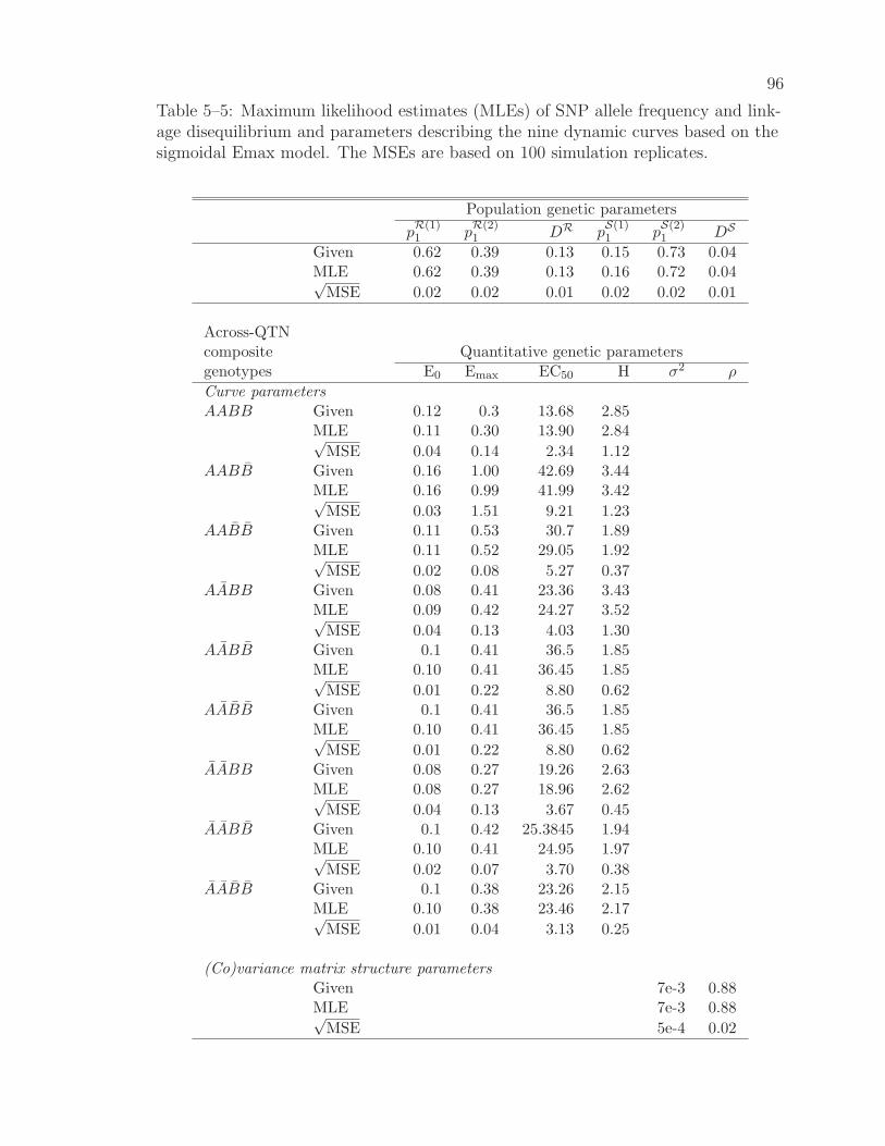
96
Table 5–5: Maximum likelihood estimates (MLEs) of SNP allele frequency and link-age disequilibrium and parameters describing the nine dynamic curves based on thesigmoidal Emax model. The MSEs are based on 100 simulation replicates.
Population genetic parameters
pR(1)1 p
R(2)1 DR p
S(1)1 p
S(2)1 DS
Given 0.62 0.39 0.13 0.15 0.73 0.04MLE 0.62 0.39 0.13 0.16 0.72 0.04√
MSE 0.02 0.02 0.01 0.02 0.02 0.01
Across-QTNcomposite Quantitative genetic parametersgenotypes E0 Emax EC50 H σ2 ρ
Curve parametersAABB Given 0.12 0.3 13.68 2.85
MLE 0.11 0.30 13.90 2.84√MSE 0.04 0.14 2.34 1.12
AABB Given 0.16 1.00 42.69 3.44MLE 0.16 0.99 41.99 3.42√
MSE 0.03 1.51 9.21 1.23AABB Given 0.11 0.53 30.7 1.89
MLE 0.11 0.52 29.05 1.92√MSE 0.02 0.08 5.27 0.37
AABB Given 0.08 0.41 23.36 3.43MLE 0.09 0.42 24.27 3.52√
MSE 0.04 0.13 4.03 1.30AABB Given 0.1 0.41 36.5 1.85
MLE 0.10 0.41 36.45 1.85√MSE 0.01 0.22 8.80 0.62
AABB Given 0.1 0.41 36.5 1.85MLE 0.10 0.41 36.45 1.85√
MSE 0.01 0.22 8.80 0.62AABB Given 0.08 0.27 19.26 2.63
MLE 0.08 0.27 18.96 2.62√MSE 0.04 0.13 3.67 0.45
AABB Given 0.1 0.42 25.3845 1.94MLE 0.10 0.41 24.95 1.97√
MSE 0.02 0.07 3.70 0.38AABB Given 0.1 0.38 23.26 2.15
MLE 0.10 0.38 23.46 2.17√MSE 0.01 0.04 3.13 0.25
(Co)variance matrix structure parametersGiven 7e-3 0.88MLE 7e-3 0.88√
MSE 5e-4 0.02

97
Genetically, drug response is a complex trait, involving multiple biochemical
pathways each controlled by different interacting genes (Marchini et al. 2005).
Traditional QTL mapping can probe the important chromosomal segments for drug
response, but is difficult to identify the causal DNA sequences of these segments.
The completion of the human genome project makes it possible to genome-wide
associate DNA sequence variants with complex phenotypes. The model proposed
in this chapter has capacity to characterize the effects of genetic factors and their
epistatic effects on drug response at the DNA sequence level.
This model has been examined through simulation studies. It can detect
significant genetic variants that control drug response and provide reasonably
precise estimates of the genetic parameters. Its application to a real example
indicates that this model will be practically useful.
There are several ways in which this model may be extended. For simplicity,
my presentation is based on the interaction between two SNP sequences from each
QTN. It is likely that the two-SNP model is too simple to characterize genetic
variants for quantitative variation. With the foundation for the two-SNP sequencing
model, this model can be extended to include an arbitrary number of SNPs whose
sequences are associated with the phenotypic variation. As shown in Lin et al.
(2005a), the multi-SNP sequencing model will encounter the problem of many
haplotypes and haplotype pairs. An AIC- or BIC-based model selection strategy
(Burnham and Andersson 1998) has been framed to determine the haplotype that is
most distinct from the rest of haplotypes in explaining quantitative variation.

CHAPTER 6MODELLING THE GENETIC ETIOLOGY OF PHARMACOKINTIC-
PHARMACODYNAMIC LINKS WITH THE ARMA PROCESS
6.1 Introduction
The genetic study of pharmacokinetics (PK) and pharmacodynamics (PD)
has received a considerable interest because of its fundamental importance in
designing personalized medications based on patients’ genetic architecture (Evans
and McLeod 2003; Weinshilboum 2003). However, each of these two processes is
complex in terms of the network of the underlying genes and their interactions
with various environmental and developmental factors. For this reason, statistical
modelling of the observed data for these two processes has been thought to be
crucial for the characterization of detailed genetic information about complex traits
(Lynch and Walsh 1998).
Unlike general complex traits, PK and PD are of dynamic nature (Hochhaus
and Derendorf 1995) which further complicates their analysis. To detect the genetic
factors for PK and PD, more advanced statistical models are needed. Although
the elucidation of the relationship between genetic control and drug response is
statistically a pressing challenge, some of key difficulties have been overcome by R.
Wu and colleagues (Ma et al. 2002; Wu et al. 2002b, 2003, 2004a, 2004b). They
have proposed a general statistical framework, i.e., functional mapping, to genome-
wide map specific QTL that determine the developmental pattern of a complex
trait.
The basic rationale of functional mapping lies in the connection between gene
action or environmental effects and drug response by parametric or nonparamet-
ric models. Functional mapping maps dynamic QTL that are responsible for a
98
99
biological or clinical process that is measured at a finite number of time points
or concentrations. A number of mathematical models have been established to
describe the PK and PD process of drug response.
The intensity of a biological response produced by a drug is related to the
concentration of the drug at the site of action which is in turn affected by a variety
of factors including genes and environments. There are four pharmacokinetic phases
which all affect drug concentration at the site of action. These phases are: (1)
absorption – the ability of a drug to enter the blood stream, (2) distribution, which
is affected by the physiochemical properties of the drug, cardiac output and blood
flow, the blood brain barrier and drug reservoirs, (3) biotransformation reactions
that alter the chemical structure of a drug, and (4) excretion is the removal of
drugs and biotransformation products from the body. A number of mathematical
functions have been proposed to describe the PK process by a set of parameters
that are related to phsyiological, clinical, physical or chemical properties of drug
(Hochhaus and Derendorf 1995).
To more precisely determine drug response, PK is integrated with PD to
quantify the relationship between pharmacodynamic actions and the dose level of
drug as well as the time after the drug is administrated (Hochhaus and Derendorf
1995). The integration of these two processes will be likely to give rise to the
therapeutically relevant results related to drug response. In this chapter, I proposed
a statistical model for detecting and identifying the genetic variants that control
the integrative PK and PD processes. This model capitalizes on the information of
DNA sequence generated by single nucleotide polymorphisms (SNPs) and embeds
mathematical functions of PK and PD processes into a mixture model framework.
This model displays unique advantages in two areas. First, the model can detect
specific DNA sequence variants rather than traditionally defined quantitative
trait loci (QTL). The utility of this model can be more effective in the discovery

100
of drugs. Second, this model is statistically vigorous in that it offers efficient
estimation of parameters that model the mean vectors and covariance matrix.
In this chapter, I develop a covariance-structuring model based on autore-
gressive moving average (ARMA) models and make use of the closed-form of the
covariance of the ARMA errors and its inverse and determinant (van der Leeuw
1994; Haddad 2004), aimed to increase the efficiency of the model. In particular,
the ARMA-based mapping model provides a general platform for vigorous mod-
elling of the covariance matrix. I perform simulation studies to investigate the
statistical behavior of the model.
6.2 Haplotyping a Complex Trait
In Lin et al. (2005), a new haplotype-based mapping approach has been
derived to detect DNA sequence variants for a biological process, such as drug
response. This new approach relies upon the the characterization of SNPs from the
entire human genome. According to results from recent studies, the human genome
can be partitioned into discrete haplotype blocks (Patil et al. 2001; Dawson et al.
2002; Gabriel et al. 2002), in each of which a limited number of SNPs, referred to
as “tag SNPs”, can explain a large fraction of the haplotype diversity.
To clearly describe this model, let us first consider two SNPs within a hap-
lotype block that are associated with the linkage disequilibrium of D in a human
population at Hardy-Weinberg equilibrium. There are two alleles 1 and 2 with the
relative proportions of p(1)1 and p
(1)2 for the first SNP as well as p
(2)1 and p
(2)2 for the
second SNP, with p(1)1 + p
(1)2 = 1 and p
(2)1 + p
(2)2 = 1. These two SNPs form 4 possible
haplotypes 11, 12, 21 and 22 whose frequencies are expressed as
pr1r2 = p(1)r1p(2)
r2+ (−1)r1+r2D,
where r1, r2 = 1, 2 denote the alleles of the two SNPs, respectively,∑2
r1=1
∑2r2=1
pr1r2 = 1 (Lynch and Walsh 1998). If the haplotype frequencies are known, then the

101
allelic frequencies and linkage disequilibrium, arrayed by the population genetic
parameter vector Ωp = p(1)r1 , p
(2)r2 , D, can be solved with the above equation.
The random combination of maternal and paternal haplotypes generates
10 distinct diplotypes expressed as [11][11], · · · , [22][22] which are sorted into
9 genotypes 11/11, · · · , 22/22 (Table 6-1). The double heterozygotic genotype
12/12 contains two possible diplotypes [11][22] and [12][21]. I use P[rm1 rm
2 ][rp1rp
2 ]
(= prm1 rm
2prp
1rp2) and Pr1r′1/r2r′2
to denote the diplotype and genotype frequencies,
respectively, and nr1r′1/r2r′2to denote the observations of various genotypes (G),
where m and p describe the maternal and paternal origins of haplotypes and
1 ≤ r1 ≤ r′1 ≤ 2, 1 ≤ r2 ≤ r′2 ≤ 2. The frequencies and observations of all genotypes,
except for genotype 12/12, are equivalent to those of the corresponding diplotypes.
I intend to associate diplotypes with inter-patient variation in a quantitative
trait based on observed phenotypic values (Y) assumed to be normally distributed.
Without loss of generality, I assume that haplotype 11 is different from the other
haplotypes, cumulatively expressed as 11, in triggering an effect on the phenotype.
Such a distinct haplotype 11 is called the reference haplotype. The reference
and non-reference haplotypes generate three combinations called the composite
genotypes. The genotypic means of the composite genotypes, µj (j = 2 for [11][11],
1 for [11][11] and 0 for [11][11]), and common residual variance within the composite
genotypes, σ2, belong to quantitative genetic parameters and are identified in
Ωq = µj, σ2.
Hence, two log-likelihood functions can be constructed, one in a multino-
mial form and another in a mixture model form, to estimate the population and
quantitative genetic parameters that are, respectively, expressed as
logL(Ωp|G) = Constant (6.1)
+2n11/11 log p11 + n11/12 log(2p11p12) + 2n11/22 log p12
102
+n12/11 log(2p11p21) + [n12/12 log(2p11p22) + (1 −)n12/12 log(2p12p21)]
+n12/22 log(2p12p22) + 2n22/11 log p21 + n22/12 log(2p21p22) + 2n22/22 log p22,
and
logL(Ωp,Ωq|Y ,G) =
n11/11∑
i=1
log f2(yi)
+
n11/12+n12/11∑
i=1
log f1(yi)
+
n11/22+n12/22+n22/11+n22/12+n22/22∑
i=1
log f0(yi)
+
n12/12∑
i=1
log[f1(yi) + (1 −)f0(yi)], (6.2)
=p11p22
p11p22 + p12p21
, (6.3)
and
fj(yi) =1√2πσ
exp
[−(yi − µj)
2
2σ2
].
I derived a closed-form solution for estimating the unknown parameters with
the EM algorithm (Lin et al. 2005). The estimates of haplotype frequencies are
based on the log-likelihood function of equation (6.1), whereas the estimates of
composite genotypic means and residual variance are based on the log-likelihood
function of equation (6.2). These two types of parameters can be estimated using
an integrative EM algorithm.
In the E step, the expected number () of diplotype [11][22] for a double
heterozygous genotype is estimated using equation (6.3), whereas the posterior
probability (Πi) with which subject i carrying the double heterozygous genotype is
diplotype [11][22] is calculated by
Πi =f1(yi)
f1(yi) + (1 −)f0(yi). (6.4)

103
Table 6–1: Possible diplotype configurations of nine genotypes at two SNPs which affect pharmacokinetics (PK) and pharma-codynamics (PD)
Parameters forRelative diplotype Haplotype composition genotypic mean vector
Genotype Diplotype Diplotype frequency freq. within genotypes 11 12 21 22 Observation PK PD
11/11 [11][11] P[11][11] = p211 1 1 0 0 0 n11/11 ke0 (Emax2, EC502)
11/12 [11][12] P[11][12] = 2p11p12 1 12
12 0 0 n11/12 ke1 (Emax1, EC501)
11/22 [12][12] P[12][12] = p212 1 0 1 0 0 n11/22 ke2 (Emax0, EC500)
12/11 [11][21] P[11][21] = 2p11p21 1 12 0 1
2 0 n12/11 ke0 (Emax1, EC501)
12/12
[11][22]
[12][21]
P[11][22] = 2p11p22
P[12][21] = 2p12p21
1 − 12 1
2(1 − ) 12(1 − ) 1
2 n12/12
ke0
ke1
(Emax1, EC501)
(Emax0, EC500)
12/22 [12][22] P[12][22] = 2p12p22 1 0 12 0 1
2 n12/22 ke1 (Emax0, EC500)
22/11 [21][21] P[21][21] = p221 1 0 0 1 0 n22/11 ke0 (Emax0, EC500)
22/12 [21][22] P[21][22] = 2p21p22 1 0 0 12
12 n22/12 ke0 (Emax0, EC500)
22/22 [22][22] P[22][22] = p222 1 0 0 0 1 n22/22 ke0 (Emax0, EC500)
= p11p22
p11p22+p12p21where p11, p12, p21 and p22 are the haplotype frequencies of [11], [12], [21], and [22], respectively. The PK and PD are
assumed to be affected by different reference haplotypes, [12] for the PK and [11] for the PD.

104
In the M step, the probabilities calculated in the previous iteration are used to
estimate the haplotype frequencies using
p11 =2n11/11 + n11/12 + n12/11 +n12/12
2n, (6.5)
p12 =2n11/22 + n11/12 + n12/22 + (1 −)n12/12
2n, (6.6)
p21 =2n22/11 + n12/11 + n22/12 + (1 −)n12/12
2n, (6.7)
p22 =2n22/22 + n22/12 + n12/22 +n12/12
2n, (6.8)
The quantitative genetic parameters are estimated using
µ2 =
∑n11/11
i=1 yi
n11/11
, (6.9)
µ1 =
∑ni=1 yi +
∑n12/12
i=1 Πiyi
n+∑n12/12
i=1 Πi
, (6.10)
µ0 =
∑ni=1 yi +
∑n12/12
i=1 (1 − Πi)yi
n+∑n12/12
i=1 (1 − Πi), (6.11)
σ2 =1
n
n11/11∑
i=1
(yi − µ2)2 +
n∑
i=1
(yi − µ1)2 +
n∑
i=1
(yi − µ0)2
+
n12/12∑
i=1
[Πi(yi − µ1)
2 + (1 − Πi)(yi − µ0)2] , (6.12)
where n = n11/12 + n12/11 and n = n11/22 + n12/22 + n22/11 + n22/12 + n22/22. Iterations
including the E and M steps are repeated among equations (6.2)–(6.12) until the
estimates of the parameters converge to stable values.
6.3 Haplotyping the Integrated PK-PD Process
6.3.1 The Likelihood Functions
Consider the same sampled population of size n as described above from which
SNPs have been genotyped. Using this population, I will test the association be-
tween SNP diplotypes and drug response. Because the effect of a drug varies with
its dosage through a pharmacodynamic process, drug effects should be measured
at a multitude of discrete dose levels. Experiencing four pharmacokinetic phases,

105
absorption, distribution, biotransformation reactions and excretion, drug concen-
tration in the body will decay with time. Thus, the degree of drug concentration
to decay with time will, in the ultimate, affect drug effect. In the other word, drug
effect is determined simultaneously by the original dosage and the time after the
drug was administrated. Let yi(d, t) be the observed drug effect for patient i at a
particular dosage d (d = 1, . . . ,D) and time t (t = 1, . . . ,T).
To detect haplotype effects on drug response to different dosage during a time
course, I need to jointly formulate multinomial- and Gaussian mixture model-based
likelihoods based on the SNP and longitudinal data. While the multinomial-based
likelihood has the same form as equation (6.1), the mixture-based likelihood needs
to incorporate longitudinal information, which is expressed, for a two-SNP model,
as
logL(Ωp,Ωq|Y ,G) =
n11/11∑
i=1
log f2(yi)
+
n11/12+n12/11∑
i=1
log f1(yi)
+
n11/22+n12/22+n22/11+n22/12+n22/22∑
i=1
log f0(yi)
+
n12/12∑
i=1
log[f1(yi) + (1 −)f0(yi)], (6.13)
where
yi =[yi(1, 1), . . . , yi(1,T)︸ ︷︷ ︸
dose 1
, . . . , yi(D, 1), . . . , yi(D,T)︸ ︷︷ ︸dose D
]
is the vector for longitudinal drug effects measured under all dosages and at
all times for patient i. Because the phenotypic measurements of drug effect are
continuously variable, it is reasonable to assume that yi follows a multivariate
normal distribution, as used in general quantitative genetic studies (Lynch and
Walsh 1998). The multivariate normal distribution for patient i who carries

106
composite genotype j is expressed as
fj(yi;uj,Σ) =1
(2π)DT|Σ|1/2exp
[−1
2(yi − uj)Σ
−1(yi − uj)′
], (6.14)
with
uj =[uj(1, 1), . . . , uj(1,T)︸ ︷︷ ︸
dose 1
, . . . , uj(D, 1), . . . , uj(D,T)︸ ︷︷ ︸dose D
](6.15)
being a vector of expected values for composite genotype j at different doses and
times.
At a particular dose d and time t, the relationship between the observation and
expected mean can be described by a linear regression model,
yi(d, t) =2∑
j=0
ξijuj(d, t) + ei(d, t), (6.16)
where ξij are the indicator variables denoted as 1 if a particular composite genotype
j is considered for individual i and 0 otherwise and ei(d, t) is the residual errors
that are iid normal with mean zero and variance σ2(d, t). The covariance matrix Σ
in equation (6.14) is factorized into different blocks, expressed as
Σ =
Σ1 . . . Σ1D
.... . .
...
ΣD1 . . . ΣD
, (6.17)
where Σ1, . . . ,ΣD are the (T × T) covariance matrices among different time
points under D different drug dose levels, respectively, and Σd1d2 is the across-dose
covariance matrix among different time points between dosage d1 and d2.
For the likelihood function (6.13), Ωp is the unknown vector for population ge-
netic parameters including SNP haplotype frequencies and Ωq contains quantitative
genetic parameters including the mean vectors of drug effects for different composite

107
genotypes at different dosages and time points and the covariance matrix among
different dosages and time points.
Although it is not perfect, the assumption of independence among D different
dosages can facilitate the modelling and analysis. With this assumption, the
likelihood of equation (6.13) can be re-written as
logL(Ωp,Ωq|Y ,G)
=
n11/11∑
i=1
log f2[yi(1)] + . . .+ log f2[yi(D)]
+
n11/12+n12/11∑
i=1
log f1[yi(1)] + . . .+ log f1[yi(D)]
+
n11/22+n12/22+n22/11+n22/12+n22/22∑
i=1
log f0[yi(1)] + . . .+ log f0[yi(D)]
+
n12/12∑
i=1
(log f1[yi(1)] + (1 −)f0[yi(1)] + . . .+ logf1[yi(D)]
+(1 −)f0[yi(D)]),
(6.18)
where
yi(1) = [yi(1, 1), . . . , yi(1,T)],
...
yi(D) = [yi(D, 1), . . . , yi(D,T)],
with dosage-specific mean vectors for composite genotype j specified by
uj(1) = [uj(1, 1), . . . , uj(1,T)],
...
uj(d) = [uj(d, 1), . . . , uj(d,T)]
...
uj(D) = [uj(D, 1), . . . , uj(D,T)],
(6.19)

108
and dosage-specific covariance matrices denoted by
Σ1, . . . ,Σd, . . . ,ΣD, (6.20)
respectively.
I will not directly estimate the elements in the mean vector and covariance
matrix, rather than estimate the parameters that model the mean-covariance struc-
tures. This will depend on two factors. First, the parameters that model dynamic
drug effects should be biologically meaningful. Second, statistical modelling of the
mean-covariance structures will be informative and can be easily implemented in
computing programs.
6.3.2 Modelling the Mean Vector
The dose- and time-dependent expected values of drug effect for composite
genotype j can be fit using a joint model of PK and PD (Hochhaus and Derendorf
1995). The PD model concerns the relationship between drug concentration (C)
and drug effect (E), which can be mathematically expressed by the Emax model
E(C) =EmaxC
EC50 + C, (6.21)
where Emax is the asymptotic (limiting) effect and EC50 is the drug concentration
that results in 50% of the maximal effect.
The PK model deals with the concentration-time profiles, which can be
described in several different ways. The PK and PD processes can be linked
directly or indirectly. The direct link applies to a situation in which the measured
concentration (or the plasma concentration cp) is proportional to drug concentration
at the effect site (biophase). The plasma concentration for a single dose in the
direct link is calculated for different cases (Hochhaus and Derendorf 1995), which

109
include
cp =
d
Vd
e−ket for intravenous (IV) bolus
dka
Vd(ka − ke)(e−ket − e−ket) for first − order absorption
ko
keVd
(ekeτ − 1)e−ket for zero − order absorption
(6.22)
where d is the bioavailable dose, Vd is the volume of distribution (which is a
constant for a known drug), ke is the elimination rate constant, ka is a first-order
absorption rate constant, ko is a zero-order absorption rate constant, τ is the
duration of zero-order absorption (τ = t during absorption and constant in the
postabsorption phase) and t is the time after the last dose was administrated.
The indirect approach for linking PK and PD assumes that there is a hy-
pothetical effect compartment and it is based on the concentration (ce) in the
compartment hypothesized to cause the drug effect. The relationship between ce
and time can be described by
ce =
dkco
Vd(kco − ke)(e−kct − e−kcot) for intravenous (IV) bolus
dkakco
Vd
[e−kct
(ka − ke)(kco − ke)+
e−kat
(ke − ka)(kco − ka)
+e−kcot
(ke − kco)(ka − kco)
]for first − order absorption
ko
keVd(kco − ke)[kco(e
keτ − 1)e−ket − kc(ekcoτ − 1)e−kcot]
for zero − order absorption
(6.23)
where kco is the rate constant for distributing drug from the compartment in which
drug concentration cause the effect.
The PK and PD processes can be jointly modelled by substituting pharma-
cokinetic model (6.22) or (6.23) to pharmacodynamic model (6.21). With such a
substitution, the effect-time-dosage relationship can be derived. For model (6.22),
the measured concentration is used, whereas for model (6.23), the concentration
hypothesized to cause the drug effect is used. For example, an integrative PK-PD

110
model in the case of an IV bolus injection without an effect compartment can be
expressed as
E(d, t) =Emaxde
−ket
EC50Vd + de−ket. (6.24)
This expression will be integrated to the mean vector of drug effects at different
time points for different dosages in equation (6.21). For a given composite genotype
j (j = 0, 1, 2), I will have the unknown vector for three parameters Ωmj=
(Emaxj, EC50j, kej) to describe time-dependent drug effects for a particular dosage d,
expressed as
uj(d) =
(Emaxjde
−kejt1
EC50jVd + de−kejt1, . . . ,
Emaxjde−kejtT
EC50jVd + de−kejtT
).
If different composite genotypes have different combinations of these parame-
ters, this implies that this sequence plays a role in governing the differentiation of
the PK-PD link. Thus, by testing for the difference of Ωmj among different compos-
ite genotypes, I can determine whether there exists a specific sequence variant that
confers an effect on the PK-PD link.
6.3.3 Modelling the Covariance Matrix
The AR and structured antedependence (SAD) models have been proposed
to model the structure of the covariance matrix for longitudinal traits measured
at multiple time points (Zimmerman and Nunez-Anton 2001; Diggle et al. 2002).
In this chapter, I will incorporate the autoregressive moving average (ARMA)
model to construct the covariance structure. There are three major advantages for
ARMA model to approximate the covariance function. First, the closed-form of
the autocovariance matrix for the ARMA process has been derived (Haddad 2004),
which allows for the expression of autocovariance function as a function of the AR
(φ1, . . . , φr) and MA coefficients (θ1, . . . , θs). Second, the derivation of the inverse
and determinant of the covariance matrix for the ARMA process by Haddad (2004)
111
has largely facilitated the computation of the likelihood function (6.18). Third, as
shown above, the ARMA model is a general form of the commonly used AR model,
which makes the ARMA-based structuring approach more useful in practice.
Given a dosage d, the residual error at time t in equation (6.16) depends on its
previous errors (deterministic) and on a random disturbance (opportunistic). For all
the following notation with dosage, such as ei(d, t), I will omit the symbol d unless
it is specified. If the dependence of ei(t) on the previous r errors is further assumed
to be linear, I can write
ei(t) = φ1ei(t− 1) + φ2ei(t− 2) + . . .+ φrei(t− r) + ǫi(t), (6.25)
where constants (φ1, . . . , φr) are called autoregressive (AR) coefficients, and ǫi(t)
is the disturbance at time t and is usually modelled as a linear combination of
zero-mean, uncorrelated random variables or a zero-mean white noise process, ǫi(t),
i.e.,
ǫi(t) = ǫi(t) + θ1ǫi(t− 1) + θ2ǫi(t− 2) + . . .+ θsǫi(t− s), (6.26)
in which ǫ(t) is a white noise process with mean 0 and variance σ2 if and only if
E[ǫ(t)] = 0, E[ǫ2(t)] = 0 for all t, and E[ε(t1), ǫ(t2)] = 0 if t1 6= t2, where E denotes
the expectation. The constants (θ1, . . . , θs) are called the moving average (MA)
coefficients. Combining equations (6.25) and (6.26) I have
ei(t) − φ1ei(t− 1) − . . .− φrei(t− r) = ǫi(t) + θ1ǫi(t− 1) + . . .+ θsǫi(t− s), (6.27)
which is defined as a zero-mean ARMA process of order r and s, or ARMA(r, s).
For a nonzero stationary ARMA process, two sequences at different time points, say
t and k, can be connected through the backward shift operator B, i.e.,
Bkei(t) = ei(t− k).

112
Define the autoregressive polynomial φ(x) and moving average polynomial θ(x) as
φ(x) = 1 − φ1x− φ2x2 − . . .− φrx
r, (6.28)
θ(x) = 1 + θ1x+ θ2x2 + . . .+ θsx
s, (6.29)
with the assumption that φ(x) and θ(x) have no common factors. equation (6.27)
can be written in form
φ(B)e(t) = θ(B)ǫ(t). (6.30)
Two special cases: When s = 0 only the AR part remain and equation (6.27)
reduces to a pure autoregressive process of order r denoted by AR(r). Similarly,
if r = 0, I obtain a pure moving average process of order s, MA(s). For these two
cases, I have
ei(t) − φ1ei(t− 1) − . . .− φrei(t− r) = φ(B)e(t) = ǫ(t) for AR(r) (6.31)
ei(t) = ǫi(t) + θ1ǫi(t− 1) + . . .+ θsǫi(t− s) = θ(B)ǫ(t) for MA(s). (6.32)
When neither r nor s is zero, an ARMA(r, s) model is sometimes referred to as a
“mixed model”.
Several efficient methods can be used to compute the exact ARMA covariance,
Σd, for a particular dosage d. Here, I use van der Leeuw’s (1994) general matrix
representation in closed-form to describe the ARMA covariance. Following van der
Leeuw (1994), I define two special types of Toeplitz matrices. The first one is a
square (T × T) Toeplitz matrix which is given for the AR and MA parameters is,
respectively, by
R =
R1 O
R2 R3
, S =
S1 O
S2 S3
(6.33)

113
where
R1 =
1 0 0 . . . 0
φ1 1 0 . . . 0
φ2 φ1 1 . . . 0
......
.... . .
...
φr−1 φr−2 φr−3 . . . 1
r×r
S1 =
1 0 0 . . . 0
θ1 1 0 . . . 0
θ2 θ1 1 . . . 0
......
.... . .
...
θs−1 θs−2 θs−3 . . . 1
s×s
,
R2 =
φr φr−1 φr−2 . . . φ1
0 φr φr−1 . . . φ2
0 0 φr . . . φ3
......
.... . .
...
0 0 0 . . . φr
0 0 0 . . . 0
......
.... . .
...
0 0 0 . . . 0
(T−r)×r
S2 =
θr θr−1 θr−2 . . . θ1
0 θr θr−1 . . . θ2
0 0 θr . . . θ3
......
.... . .
...
0 0 0 . . . θr
0 0 0 . . . 0
......
.... . .
...
0 0 0 . . . 0
(T−s)×s
R3 =
1 0 0 . . . 0 0 . . . 0
φ1 1 0 . . . 0 0 . . . 0
φ2 φ1 1 . . . 0 0 . . . 0
......
.... . .
......
. . ....
φr φr−1 φr−2 . . . 1 0 . . . 0
φr φr−1 φr−2 . . . φ1 1 . . . 0
......
.... . .
......
. . ....
0 0 0 φr φr′ φr′−1 . . . 1
(T−r)×(T−r)

114
S3 =
1 0 0 . . . 0 0 . . . 0
θ1 1 0 . . . 0 0 . . . 0
θ2 θ1 1 . . . 0 0 . . . 0
......
.... . .
......
. . ....
θs θs−1 θs−2 . . . 1 0 . . . 0
θs θs−1 θs−2 . . . θ1 1 . . . 0
......
.... . .
......
. . ....
0 0 0 θs θs′ θs′−1 . . . 1
(T−s)×(T−s).
The second defined matrix has dimension T × r for the AR parameters and
T × s for the MA parameters, whose upper parts are a square (r × r) or (s × s)
Toeplitz matrix. For these two types of parameters, I define, respectively,
U =
U1
O
, V =
V1
O
, (6.34)
where
U1 =
φr φr−1 . . . φ1
0 φr . . . φ2
......
. . ....
0 0 . . . φr
r×r
, V1 =
θs θs−1 . . . θ1
0 θs . . . θ2
......
. . ....
0 0 . . . θs
s×s
Given the error vectors,
e = [e(t− 1), e(t− 2), . . . , e(t− r + 1), e(t− r)]T ,
ǫ = [ǫ(s− 1), ǫ(s− 2), . . . , ǫ(t− s+ 1), ǫ(t− s)]T ,
I define the corresponding auxiliary vectors by
e = [e(−r + 1), e(−r + 2), . . . , e(−1), e(0)]T ,
ǫ = [ǫ(−s+ 1), ǫ(−s+ 2), . . . , ǫ(−1), ǫ(0)]T .

115
I then write equation (6.27) in matrix form
[U R]
e
e
= [V S]
ǫ
ǫ
or Re = Vǫ− Sǫ− Ue,
from which a series of matrix operations can be performed to prove that the
covariance matrix Σd corresponding to the ARMA(r, s) error specification is
solution to the equation (van der Leeuw 1994),
RΣdRT = SST + VVT + [U O]Σd[U O]T − [V O]STΣ−T
d [U O]T
−[U O]R−1S[V O]T . (6.35)
As shown in van der Leeuw (1994), if the invertibility condition for the AR part
holds, the covariance equation (6.35) has an unique solution, which is
Σd = R−1[SST + (RV − SU)(PT1 P1 − UT
1 U1)−1(RV − SU)T ]R−T . (6.36)
By substituting R = I and Q = O in equation (6.35), the covariance matrix for the
MA(s) model is obtained as
Σd = SST + VVT . (6.37)
By substituting S = O and V = O, next premultiplying both sides of equation
(6.36) and postmultiplying by its transpose, the covariance matrix for the AR(r)
model is derived as
Σd = (RTR − UUT )−1. (6.38)
Based on the expression for the inverse of the sum of two matrices (Rao 1973), I
obtain the inverse of Σd as
Σ−1d = RTS−T[IT − M(MTM + RT
1 R1 − U1UT1 )−1MT ]S−TR, (6.39)

116
with M = S−1RV − U. Given that the value of the determinant of S−1R is equal to
one, I have
|Σd| =
∣∣∣∣∣∣∣IT − S−1
R1V1 − S1U1
O
(RT
1 R1 − U1UT1 )−1
R1V1 − S1U1
O
T
S−1
∣∣∣∣∣∣∣(6.40)
=∣∣∣Ir + (RT
1 R1 − U1UT1 )−1(R1V1 − S1U1)
T ST1 S1(R1V1 − S1U1)
∣∣∣ , (6.41)
where S1 is the (T × r) matrix, consisting of the first r columns of S−1. For the
AR(r) model, the determinant is reduced to
∣∣(RT1 R1 − U1U
T1 )−1
∣∣ ,
which is independent of T.
With the above derivations, it can be seen that the parameters that model the
covariance matrix are arrayed by Ωv = φ1(d), . . . , φr(d), θ1(d), . . . , θs(d), σ2dD
d=d1
for D dose levels when the ARMA(r, s) model is implemented. The unknown vector
can reduce to the AR(r) or MA(s) model, depending on practical problems.
6.3.4 Computational Algorithms
I implemented the EM algorithm, originally proposed by Dempster et al.
(1977), to obtain the maximum likelihood estimates (MLEs) of three groups of
unknown parameters in the integrated sequence and function mapping model,
that is, the marker population parameters (Ωp), the curve parameters (Ωmj) that
model the mean vector, and the parameters (Ωv) that model the structure of the
covariance matrix. These unknowns are denoted by Ω = (Ωp,Ωmj,Ωv). A detailed
description of the EM algorithm was given in Wu et al. (2002b, 2004b) and Ma et
al. (2002).
As described for single trait mapping, I implement the E step to calculate the
expected number () of diplotype [11][22] contained in the double heterozygote

117
12/12 and the posterior probability (Πi) of double heterozygotic patient i who
carries diplotype [11][22]. In the M step, I use the calculated and Πi values to
estimate the haplotype frequencies using equations (6.5) – (6.8). But in this step, I
encounter a considerable difficulty in deriving the log-likelihood equations for Ωmj
and Ωv because they are contained in complex nonlinear equations. Zhao et al.
(2004) implemented the simplex method as advocated by Nelder and Mead (1965)
to the estimation process of functional mapping, which can strikingly increase
computational efficiency. In this chapter, the simplex algorithm is embedded in the
EM algorithm above to provide simultaneous estimation of haplotype frequencies
and curve parameters and matrix-structuring parameters.
6.3.5 Model for an Arbitrary Number of SNPs
The idea for sequencing drug response has been described for a two-SNP
model. It is possible that the two-SNP model is too simple to characterize genetic
variants for variation in drug response. I have extended this model to include an
arbitrary number of SNPs whose sequences are associated with drug response
variation. A key issue for the multi-SNP sequencing model is how to distinguish
among 2w−1 different diplotypes for the same genotype heterozygous at w loci.
The relative frequencies of these diplotypes can be expressed in terms of haplotype
frequencies. The integrative EM algorithm can be employed to estimate the MLEs
of haplotype frequencies. Bennett (1954) provided a general formula for expressing
haplotype frequencies in terms of allele frequencies and linkage disequilibria of
different orders. The MLEs of the latter can be obtained by solving a system of
equations.
6.4 Hypothesis Tests
This model allows for the tests of a number of biologically or clinically mean-
ingful hypotheses at the interface between gene actions and drug response. The
existence of specific genetic variants affecting an integrated PK-PD process can be

118
tested by formulating the following hypotheses,
H0 : Ωmj≡ Ωm, j = 2, 1, 0
H1 : at least one of the equalities above does not hold,
(6.42)
where H0 corresponds to the reduced model, in which the data can be fit by a
single drug response curve, and H1 corresponds to the full model, in which there
exist different dynamic curves to fit the data. The test statistic for testing the
hypotheses in equation (6.42) is calculated as the log-likelihood ratio (LR) of the
reduced to the full model:
LR = −2[logL(Ω|y,G) − logL(Ω|y,G)], (6.43)
where Ω and Ω denote the MLEs of the unknown parameters under H0 and H1,
respectively. The LR is asymptotically χ2-distributed with 8 degrees of freedom. An
empirical approach for determining the critical threshold is based on permutation
tests, as advocated by Churchill and Doerge (1994). By repeatedly shuffling the
relationships between marker genotypes and phenotypes, a series of the maximum
log-likelihood ratios are calculated, from the distribution of which the critical
threshold is determined.
An alternative approach for testing the existence of DNA sequence variants
that are responsible for the integrated PK-PD process can be based on the volume
under the landscape (V UL). The V UL for a landscape for a given composite
genotype j can be calcualted by
V ULj =
∫ dD
d1
∫ tT
t1
Emaxjde−kejt
EC50jVd + de−kejtdt · dd
=
∫ dD
d1
[Emaxj
kej
ln
(1 +
d
EC50jVd
)]dd as t1 → 0 and tT → ∞ (6.44)
The null hypothesis for the existence of a significant DNA sequence variant based

119
on the V UL is expressed as V ULj ≡ V UL. A similar LR test statistic can be
calculated using equation (6.43) for statistical testing.
Although I here assume the same PK (ke) and PD parameters (Emax and EC50)
for different dose levels, this model can be generalized to allow these parameters to
vary over dosage. It is possible that different reference haplotypes are operational
for pharmacodynamic effects under different dosage, which is the cause of haplotype
× dosage interaction effects. For any pair of dosages, d1 and d2, this haplotype ×
dosage interaction can be tested by formulating the hypothesis tests of drug effects:
H0 : E0(d1, t) − E0(d2, t) = E1(d1, t) − E1(d2, t) = E2(d1, t) − E2(d2, t)
H1 : at least one of the equalities above does not hold,
(6.45)
where Ej(d1, t) or Ej(d2, t) is the effect-time profile for composite genotype j under
dosage d1 or d2, respectively, which is described by equation (6.24). The parameters
under the H0 of (6.44) can be estimated by posing appropriate constraints as shown
in Lin et al. (2005). If the null hypothesis is rejected, this means that the same
haplotype may trigger different impacts on drug effect under different dosages.
Similarly, I can make a hypothesis test about haplotype × time interactions.
The null hypothesis for this test is based on the effect-dosage profile with the
relationship like E0(d, t1) − E0(d, t2) = E1(d, t1) − E1(d, t2) = E2(d, t1) − E2(d, t2) for
two given time points t1 and t2. In addition, individual curve parameters, such as
Emax, EC50 and ke, can be tested. The tests of these parameters are important for
the design of personalized drugs to control particular diseases.
6.5 Results
To examine the statistical properties of the genetic model for the integrated
PK-PD process, I perform a simulation study in which a landscape of drug effect
as a function of dose level and time is simulated. Figure 6-1 is a typical example
generated by equation (6.24) in which three landscapes each presenting a different

120
010
2030
4050
100
101
102
103
0
0.1
0.2
0.3
0.4
0.5
0.6
0.7
0.8
0.9
1
Time (h)
Dose (mg)
Effe
ct (
%)
Figure 6–1: Landscapes of drug effects varying as a function of dosage and time forthree hypothesized composite genotypes.
composite genotype over-crosses, suggesting that there are interactions between
haplotypes and dosages and times.
The simulation will be based on the ARMA(r, s) model (6.30). For compu-
tational simplicity, I only consider the AR(1) parameters so that only φ and σ2
are used to model the structure of the residual covariance matrix. A total of 200
unrelated individuals are assumed to randomly sample from a human population
at Hardy-Weinberg equilibrium with respect to haplotypes. Table 6-1 tabulates
the distribution of the frequencies of haplotypes constructed by two SNPs in terms
of allele frequencies and linkage disequilibrium. The diplotypes derived from four
haplotypes at these two SNPs affect the integrated PK and PD process. As two

121
different processes, it is possible that PK and PD are controlled by different DNA
sequence variants. By assuming arbitrarily different reference haplotypes for the
PK (say 12) and PD (say 11), I can specify the mean vectors for each composite
genotype (Table 6-1).
Longitudinal PK and PD data are simulated at 6 time points for 4 dose levels
under the multivariate normal distribution using the PK (ke) and PD curve pa-
rameters (Emax and EC50) for the respective three composite genotypes, as given
in Table 6-2. These curve parameters are determined in the ranges of empirical
estimates of these parameters from pharmacological studies (Hochhaus and Deren-
dorf 1995). Figure 6-1 illustrates the differences in the effect-concentration-time
landscape among three composite genotypes. Using the genetic variance due to the
composite genotypic difference in the volume under landscape, I calculate the resid-
ual variances under different heritability levels (H2 = 0.1 and 0.4). These residual
variances, plus given residual correlations, form a structured residual covariance
matrix Σ.
The population genetic parameters of the SNPs can be estimated with rea-
sonably high precision using the closed-form solution approach (Table 6-2). The
estimates of these parameters are only dependent on sample size and are not re-
lated to the size of heritability. This model allows for the identification of correct
reference haplotypes for the PK and PD processes. By considering all possible
combination of reference haplotypes for these two processes, I calculate the LR
test statistics using equation (6.43) for each combination. The maximum LR value
corresponds to the case in which the reference haplotypes for these two processes
are consistent with the given ones (see Table 6-2).
Figure 6-2 describes different shapes of the PK and PD from the three com-
posite genotypes with a comparison between the given and estimated curves under
a selected dose level. The estimated curves are consistent with the given curves,

122
Table 6–2: Maximum likelihood estimates of SNP population genetic parameters(allele frequencies and linkage disequilibrium), the curve parameters and matrix-structuring parameters for pharmacokinetics and pharmacodynamics responses. Thenumbers in parentheses are the square root of MSEs for the estimates.
Composite HeritabilityParameters genotype True value 0.1 0.4
Population genetic parameters
p(1)1 0.60 0.60(0.02) 0.60(0.02)
p(2)1 0.60 0.60(0.03) 0.60(0.02)D 0.08 0.08(0.01) 0.08(0.01)
Curve parameters: Pharmacokineticske [12][12] 0.20 0.20(0.02) 0.21(0.02)
[12][12] 0.30 0.30(2e-3) 0.30(9e-4)[12][12] 0.40 0.40(3e-3) 0.40(1e-3)
Curve parameters: PharmacodynamicsEmax [11][11] 0.60 0.60(6e-3) 0.60(3e-3)
[11][11] 0.80 0.80(5e-3) 0.80(2e-3)[11][11] 1.00 1.00(7e-3) 0.10(3e-3)
EC50 [11][11] 0.01 0.01(2e-4) 0.01(1e-4)[11][11] 0.02 0.02(2e-4) 0.02(1e-4)[11][11] 0.03 0.03(3e-4) 0.03(1e-4)
Matrix-structuring parametersDose d = 1ρ 0.70 0.70(0.02) 0.69(0.10)σ2 9e-5 9e-5(1e-5)
1e-5 1e-5(4e-6)Dose d = 10ρ 0.70 0.70(0.02) 0.71(0.09)σ2 2e-3 2e-3(2e-3)
3e-4 4e-4(3e-4)Dose d = 100ρ 0.70 0.70(0.02) 0.72(0.06)σ2 0.02 0.02(0.01)
3e-3 3e-3(4e-3)Dose d = 1000ρ 0.70 0.70(0.02) 0.72(0.07)σ2 0.05 0.05(0.04)
0.01 0.01(0.01)

123
suggesting that this model can provide reasonable estimates of PK and PD curves.
The parameters for the PK and PD models of each composite genotype can be
estimated accurately and precisely (Table 6-2). As expected, the estimation preci-
sion (assessed by MSEs) increases remarkably when the heritability increases from
0.1 to 0.4. The estimates of the AR(1) parameters that model the structure of
the covariance matrix Σ also display reasonably high precision (Table 6-2). But it
seems that their estimation precision is independent of the size of heritability.
In each of 100 simulations, I calculate the log-likelihood ratios (LR) for
the hypothesis test of the presence of a genetic variant affecting both PK and
PD processes. The LR values in each simulation under both heritability levels
are strikingly higher than the critical threshold estimated from 100 replicates
of simulations under the null hypothesis that there is no PK/PD-associated
genetic variant. This suggests that this model has enough power to detect the
genetic variant under given SNPs, curve and matrix-structuring parameters for the
simulation.
6.6 Discussion
The genetic control of pharmacokinetics (PK) and pharmacodynamics (PD) is
one of the most important aspects in current pharmacogenomic or pharmacogenetic
research (Watters and Mcleod 2003). Historically, this kind of study has been
complicated by two factors. First, there was no adequate information available
about the DNA structure and organization of the human genome. The recent
release of the haplotype map (HapMap) constructed by SNPs (The International
HapMap Consortium 2003) has made it possible to identify polymorphic sites at the
DNA sequence level and further associate the DNA sequence variants with complex
diseases or drug response. Second, drug response is a dynamic process, affected by
time and drug concentration. It is insufficient to study the genetic basis for drug
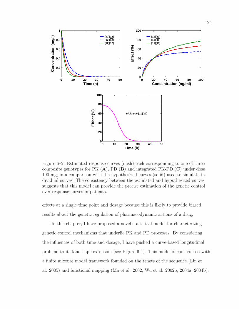
124
0 10 20 30 40 500
0.2
0.4
0.6
0.8
1
[12][12][12][12][12][12]
Time (h)
Co
nce
ntr
atio
n (
mg
/l)
0 20 40 60 80 1000
20
40
60
80
100
[11][11][11][11][11][11]
Concentration (ng/ml)
Eff
ect
(%)
0 10 20 30 40 500
20
40
60
80
100
Diplotype [11][12]
Time (h)
Eff
ect
(%)
Figure 6–2: Estimated response curves (dash) each corresponding to one of threecomposite genotypes for PK (A), PD (B) and integrated PK-PD (C) under dose100 mg, in a comparison with the hypothesized curves (solid) used to simulate in-dividual curves. The consistency between the estimated and hypothesized curvessuggests that this model can provide the precise estimation of the genetic controlover response curves in patients.
effects at a single time point and dosage because this is likely to provide biased
results about the genetic regulation of pharmacodynamic actions of a drug.
In this chapter, I have proposed a novel statistical model for characterizing
genetic control mechanisms that underlie PK and PD processes. By considering
the influences of both time and dosage, I have pushed a curve-based longitudinal
problem to its landscape extension (see Figure 6-1). This model is constructed with
a finite mixture model framework founded on the tenets of the sequence (Lin et
al. 2005) and functional mapping (Ma et al. 2002; Wu et al. 2002b, 2004a, 2004b).
125
This model has particular power to discern the discrepancy between the genetic
mechanisms for PK and PD. With the aid of HapMap, this model allows for the
genome-wide scan of genetic variants that responsible for these two different but
physiologically related processes.
Unlike traditional statistical models in similar areas, my model can directly
detect DNA sequences that code PK and PD processes. Thus, genetic information
extracted from observed data by this model is more informative and precise than
that from traditional approaches. In particular, clinally meaningful mathematical
functions (Hochhaus and Derendorf 1995; Giraldo 2003; McClish and Roberts 2003)
have been integrated to a statistical framework, thus display significant advantages.
First, it facilitates statistical analysis and strengthens power to detect significant
genetic variants because fewer parameters are needed to be estimated, as opposed
to traditional multivariate analysis. Second, the results it produces are close to
biological realm given that the mathematical functions used are founded on a firm
understanding of pharmacology (reviewed in Derendorf and Meibohm 1999). Based
on differences in the PK-PD landscape, as shown in Figure 6-1, I can test for the
genetic control regarding how pharmacokinetic actions change over time (the time
surface) and how pharmacodynamic effects vary over dosage (the dosage surface) by
estimating the slopes of each surface. The statistical power of this model is further
increased by the attempt to structure the covariance matrix with autoregressive
models (Diggle et al. 2002).
This model has been relied upon the modelling and analysis of the residual
covariance matrix. In this chapter, I have for the first time incorporated a time
series model – autoregressive moving average (ARMA) model – into the mixture
model context. The ARMA model has been commonly used in econometric research
aimed to approach the time-dependent influence of errors (van der Leeuw 1994).
This model is very flexible in that any order of a polynomial that model dynamic

126
errors can be determined. Furthermore, there is a surprisingly simple form for
its description of the covariance matrix. The closed forms of the inverse and
determinant of the matrix can greatly enhance computational efficiency (van der
Leeuw 1994; Haddad 2004). With the ARMA model, the AR(1) model that has
been used to model the covariance structure (Ma et al. 2002; Wu et al. 2004a,
2004b; Lin et al. 2005) can be viewed as a special case.
As usual, simulation studies have been employed to investigate the statistical
behavior of this model. The results suggest that it can provide accurate and
precise estimates of the response curves for both PK and PD even when the
heritability is modest. Different drug response curves, as simulated for different
composite genotypes (Figure 6-1), can offer scientific guidance for determining the
optimal dose and optimal dosage form that display favorable drug effects based on
individual’s genetic background. It should be noted that this model was derived
on the basis of a simple clinical design in which a single cohort is assumed, with
equally concentration intervals for every patient. This model can be extended to
a case-control study by allowing haplotype frequencies and haplotype effects to be
different between the case and control groups. A series of hypothesis tests regarding
between-group differences can be formulated to detect specific haplotypes that
are responsible for drug response. This model can also be extended to consider
various measurement schedules, in particular with uneven concentration lags
varying from patient to patient. For these irregular measurement schedules, it is
needed to formulate individualized likelihood functions when the mean vector and
covariance matrix are modelled (see Nunez-Anton and Woodworth 1994). With
these extensions, my model will assist in the discovery and characterization of a
network of genes that influence drug response in terms of pharmacokinetics and
pharmacodynamics.

CHAPTER 7CONCLUSIONS AND PROSPECTS
7.1 Summary
The information about how DNA sequence varies across the human genome
is crucial for unravelling the genetic basis of drug response. The overall objective
of this dissertation is to develop statistical models for directly detecting and
characterizing specific DNA sequence variants that are responsible for drug response
under various problem settings. The basic tenets of these models are to integrate
mathematical aspects of drug response and SNP-based haplotype blocking theory
into a statistical mixture model-based mapping framework.
In Chapter 2, a conceptual model was derived as the general framework for
my series of studies. This model was employed to a pharmacogenetic study of
cardiovascular disease, leading to the detection of a particular haplotype that
exhibits a different effect on heart rate curve compared to the rest of haplotypes.
This simple model was then extended to include two different but related processes,
drug efficacy and drug toxicity in Chapter 3. Simulation studies suggest that the
extended model has power to test whether there exist different DNA sequence
variants that govern these two drug responses and how different different variants
affect efficacy and toxicity in a coherent way.
Because genetic interactions are thought to be a ubiquitous biological phe-
nomenon and play a pivotal rule in controlling many important human diseases as
well as drug response. In Chapter 4 and 5, two models were derived for the char-
acterization of different DNA sequences that interact in a coordinated manner to
regulate the complex disease and the dynamic process of drug effects, respectively.
127
128
The models provide quantitative frameworks for testing the additive × additive,
additive × dominant, dominant × additive and dominant × dominant interaction
effects between different QTN sequences from haplotype blocks. The significant
sequence-sequence interactions were effectively detected in a worked example.
Chapter 6 provides a high-dimensional statistical model for unveiling the
genetic secrets for drug response by integrating pharmacokinetics (PK) and
pharmacodynamics (PD) into a genetic mapping framework. Simulation studies
were performed to test how the specific haplotypes affect differently the effect of
body on the drug (PK) and the effect of drug on the body (PD) simultaneously.
Perhaps, the most significant strength of my dissertation is in its nature
of cutting edge research toward a historically complicated biomedical problem.
The theoretical models proposed in my dissertation were derived on the basis
of biomedical principles and have potentially much broader applications. The
statistical contributions of my dissertation include the elegant derivation for a
closed form solution for estimating allelic frequencies and linkage disequilibria
for sequence variants that control drug response within the context of the EM
algorithm as well as the integration of the EM-simplex algorithm for estimating the
genetic action and interactions of these variants.
In my dissertation, I also attempt to make a contribution to pharmacoge-
netic and pharmacogenomic research. Different from candidate gene approaches,
my models can be directly employed to identify DNA sequences without prior
knowledge about pharmacodynamic mechanisms of drug effects. In particular, my
models will allow for the genome-wide search for genetic variants that control drug
response. Also, because the derivations of my models are based on the biochemical
principles behind drug response, the results from them should be biologically more
relevant and clinically more effective.

129
By integrating mathematical, statistical and computer languages into the
genetic control of pharmacodynamic and pharmacokinetic processes, my models
provide a quantitative and testable framework for asking and addressing biological
problems at the interplay between gene action and drug response.
7.2 Future Directions
Although this dissertation has for the first time documented basic models for
the genetic study of drug response, there is still much room for further derivations
and modelling. Below, I pinpoint several areas in which further effort can make a
visible progress.
7.2.1 Gene-Environment Interaction
A wealth of evidence has suggested that the interactions between genes and
various environmental or developmental signals can exert pronounced effects on
drug response. A further interaction model, incorporated with environmental
impacts on differentiation in drug response, can be derived to provide a testable
framework for unravelling the mechanisms of how sequence variants interact with
environment to mediate drug response.
A high-dimensional gene-environment interaction model can be derived to
characterize differentiated genetic mechanisms for the responsiveness of the same
drug to different environmental factors. The results from such interaction models
can help to design an optimal drug and optimal dose for treating a disease based
on coordinated interactions between a patient’s genetic architecture and the
environment of the patient.
7.2.2 Case-Control Study
Genes for drug response may be segregating differently between normal
(control) and affected (case) populations. This population-dependent segregation
patterns of DNA sequence variants can be incorporated into a series of procedures

130
to test how DNA variants operate differently in case or control populations to
govern drug response.
The case-control model can detect the differences of the frequencies and effects
of causal haplotypes for a QTN between different populations. This information
helps to precisely compare the population-dependent differences in DNA structure
and organization of QTN thought to regulate drug response.
7.2.3 Dose-Dependency of Allometric Scaling Performance
The use of a drug would give rise to alternations in a patient’s physiological
metabolism which has been found to universally scale as a multiple of quarters
of body mass (West at al. 1997, 1999). The performance of allometric scaling
of dose as a power of body weight remains untested in many cases. However, its
integration with a genetic mapping study like this would produce exciting results in
pharmacogenetic research.
The motivation of size to be incorporated into an analysis of drug effect
results from known biological principles. A great many physiological, structural
and time related variables scale predictably within and between species with
weight exponents of 0.75, 1 and 0.25, respectively. West at al. (1997, 1999) have
used fractional geometry to mathematically explain this phenomenon. The 3/4
power law for metabolic rates was derived from a general model that describes
how essential materials are transported through space-filled fractional networks of
branching tubes. These design principles are independent of detailed dynamics and
explicit models and should apply to virtually all organisms.
7.2.4 Missing Data Problem
In pharmacogenetic research, missing data are almost always a problem. Data
can be missing completely at random (MCAR), missing at random (MAR), or
missing not at random (MNAR). Statistical models have been available for handling
missing data with MCAR, but have not been sufficiently developed for the other

131
two missing mechanisms. It appears that pattern-mixture models can be used to
solve some problems related to MAR and MNAR. The implementation of pattern-
mixture models in the genetic mapping with DNA sequence variants would be
powerful to characterize the genetic regulation of drug response with non-ignorable
data.
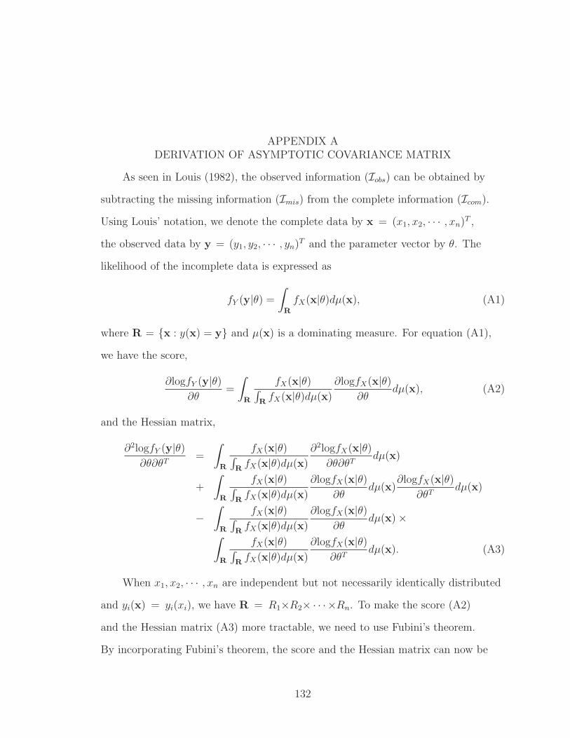
APPENDIX ADERIVATION OF ASYMPTOTIC COVARIANCE MATRIX
As seen in Louis (1982), the observed information (Iobs) can be obtained by
subtracting the missing information (Imis) from the complete information (Icom).
Using Louis’ notation, we denote the complete data by x = (x1, x2, · · · , xn)T ,
the observed data by y = (y1, y2, · · · , yn)T and the parameter vector by θ. The
likelihood of the incomplete data is expressed as
fY (y|θ) =
∫
R
fX(x|θ)dµ(x), (A1)
where R = x : y(x) = y and µ(x) is a dominating measure. For equation (A1),
we have the score,
∂logfY (y|θ)∂θ
=
∫
R
fX(x|θ)∫RfX(x|θ)dµ(x)
∂logfX(x|θ)∂θ
dµ(x), (A2)
and the Hessian matrix,
∂2logfY (y|θ)∂θ∂θT
=
∫
R
fX(x|θ)∫RfX(x|θ)dµ(x)
∂2logfX(x|θ)∂θ∂θT
dµ(x)
+
∫
R
fX(x|θ)∫RfX(x|θ)dµ(x)
∂logfX(x|θ)∂θ
dµ(x)∂logfX(x|θ)
∂θTdµ(x)
−∫
R
fX(x|θ)∫RfX(x|θ)dµ(x)
∂logfX(x|θ)∂θ
dµ(x) ×∫
R
fX(x|θ)∫RfX(x|θ)dµ(x)
∂logfX(x|θ)∂θT
dµ(x). (A3)
When x1, x2, · · · , xn are independent but not necessarily identically distributed
and yi(x) = yi(xi), we have R = R1×R2× · · · ×Rn. To make the score (A2)
and the Hessian matrix (A3) more tractable, we need to use Fubini’s theorem.
By incorporating Fubini’s theorem, the score and the Hessian matrix can now be
132
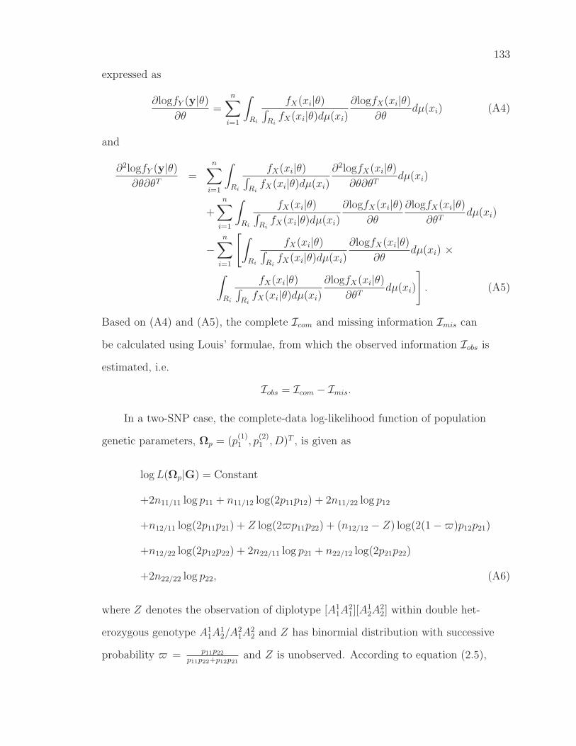
133
expressed as
∂logfY (y|θ)∂θ
=n∑
i=1
∫
Ri
fX(xi|θ)∫RifX(xi|θ)dµ(xi)
∂logfX(xi|θ)∂θ
dµ(xi) (A4)
and
∂2logfY (y|θ)∂θ∂θT
=n∑
i=1
∫
Ri
fX(xi|θ)∫RifX(xi|θ)dµ(xi)
∂2logfX(xi|θ)∂θ∂θT
dµ(xi)
+n∑
i=1
∫
Ri
fX(xi|θ)∫RifX(xi|θ)dµ(xi)
∂logfX(xi|θ)∂θ
∂logfX(xi|θ)∂θT
dµ(xi)
−n∑
i=1
[∫
Ri
fX(xi|θ)∫RifX(xi|θ)dµ(xi)
∂logfX(xi|θ)∂θ
dµ(xi) ×
∫
Ri
fX(xi|θ)∫RifX(xi|θ)dµ(xi)
∂logfX(xi|θ)∂θT
dµ(xi)
]. (A5)
Based on (A4) and (A5), the complete Icom and missing information Imis can
be calculated using Louis’ formulae, from which the observed information Iobs is
estimated, i.e.
Iobs = Icom − Imis.
In a two-SNP case, the complete-data log-likelihood function of population
genetic parameters, Ωp = (p(1)1 , p
(2)1 , D)T , is given as
logL(Ωp|G) = Constant
+2n11/11 log p11 + n11/12 log(2p11p12) + 2n11/22 log p12
+n12/11 log(2p11p21) + Z log(2p11p22) + (n12/12 − Z) log(2(1 −)p12p21)
+n12/22 log(2p12p22) + 2n22/11 log p21 + n22/12 log(2p21p22)
+2n22/22 log p22, (A6)
where Z denotes the observation of diplotype [A11A
21][A
12A
22] within double het-
erozygous genotype A11A
12/A
21A
22 and Z has binormial distribution with successive
probability = p11p22
p11p22+p12p21and Z is unobserved. According to equation (2.5),

134
haplotype frequencies are
p11 = p(1)1 p
(2)1 +D,
p12 = p(1)1 (1 − p
(2)1 ) −D,
p21 = (1 − p(1)1 )p
(2)1 −D,
p22 = (1 − p(1)1 )(1 − p
(2)1 ) +D.
on the other hand, the population genetic parameters can be solved once we know
the estimates of haplotype frequencies, that are
p(1)
1 = p11 + p12 (A7)
p(2)
1 = p11 + p21 (A8)
D = p11 − p 211 − p11p12 − p11p21 − p12p21 (A9)
Let M1(3×1) = ∂ log L(Ωp|G)
∂Ωp=
(∂ log L(Ωp|G)
∂p(1)1
, ∂ log L(Ωp|G)
∂p(2)1
, ∂ log L(Ωp|G)
∂D
)T
, then
M111 =2n11/11p
(2)1
p11
+n11/12[p
(2)1 p12 + p11(1 − p
(2)1 )]
p11p12
+2n11/22(1 − p
(2)1 )
p12
+n12/11(p
(2)1 p21 − p11p
(2)1 )
p11p21
+Z[2p
(2)1 p22 − 2(1 − p
(2)1 )p11 −S1]
p11p22
−(n12/12 − Z)(p(2)1 − p11 − p21 −S1)
p12p21
+n12/22(1 − p
(2)1 )(p22 − p12)
p12p22
−2n22/11p(2)1
p21
− n22/12[p(2)1 p22 + p21(1 − p
(2)1 )]
p21p22
− 2n22/22(1 − p(2)1 )
p22
,
M121 =2n11/11p
(1)1
p11
+n11/12[p
(1)1 p12 − p11(1 − p
(1)1 )]
p11p12
− 2n11/22p(1)1
p12
+n12/11[p
(1)1 p21 + p11(1 − p
(1)1 )]
p11p21
+Z[2p
(1)1 p22 − 2(1 − p
(1)1 )p11 −S2]
p11p22
−(n12/12 − Z)(p(1)1 − p11 − p12 −S2)
p12p21
− n12/22[p(1)1 (p22 − p12) + p12]
p12p22
+2n22/11(1 − p
(1)1 )
p21
+n22/12(1 − p
(1)1 )(p22 − p21)
p21p22
− 2n22/22(1 − p(1)1 )
p22
,

135
M131 =2n11/11
p11
+n11/12(p12 − p11)
p11p12
− 2n11/22
p12
+n12/11(p21 − p11)
p11p21
+Z[2(p22 + p11) −S3)]
p11p22
− (n12/12 − Z)[1 +S3]
p12p21
−n12/22(p22 − p11)
p12p22
− 2n22/11
p21
− n22/12(p22 − p21)
p21p22
+2n22/22
p22
,
where S1 = p(2)1 (p22−p12)+(1−p(2)
1 )(p21−p11), S2 = p(1)1 (p22−p21)+(1−p(1)
1 )(p12−p11)
and S3 = p11 + p22 − p12 − p21.
Let M2(3×3) = ∂2 log L(Ωp|G)
∂Ωp∂ΩTp
, therefore
Icomp = E −M2Ωp=Ωp
and
Imisp = E
(M1) (M1)T
Ωp=Ωp
−
E (M1)Ωp=ΩpE (M1)
TΩp=Ωp
where G = (n11/11, n11/12, · · · , n22/22) is the vector of observations and Ωp are the
MLEs of population parameters calculated using equations (A7) – (A9).
Similarly, we also can estimate the asymptotic variance-covariance matrix
for quantitative genetic parameters (Ωq). In two-SNP case, the complete-data
log-likielihood function of Ωq is expressed as
logL(Ωq|Ycom,G,Ωp) =
n11/11∑
i=1
log f2(yi)
+
n11/12+n12/11∑
i=1
log f1(yi)
+
n11/22+n12/22+n22/11+n22/12+n22/22∑
i=1
log f0(yi)
+
n12/12∑
i=1
Zi log[f1(yi)]
+
n12/12∑
i=1
(1 − Zi) log[(1 −)f0(yi)],

136
where Zi is the indicator variable denoted as 1 if individual i has diplotype
[A11A
21][A
12A
22] within genotype A1
1A12/A
21A
22 and 0 otherwise. Zi has Bernoulli
distribution with successive probability and Zi is unobserved. Hence,
Icomq = E
−∂
2 logL(Ωq|Ycom,G,Ωp)
∂Ωq∂ΩTq
|Yobs
Ωp=Ωp, Ωq=Ωq
Imisq = E
[∂ logL(Ωq|Ycom,G,Ωp)
∂Ωq
]×
[∂ logL(Ωq|Ycom,G,Ωp)
∂Ωq
]T
|Yobs
Ωp=Ωp, Ωq=Ωq
−
E
[∂ logL(Ωq |Ycom,G,Ωp)
∂Ωq
|Yobs
]
Ωp=Ωp, Ωq=Ωq
×
E
[∂ logL(Ωq |Ycom,G,Ωp)
∂Ωq
|Yobs
]T
Ωp=Ωp, Ωq=Ωq
where Ωq are the MLEs of quantitative parameters derived from simplex algorithm.

APPENDIX BDERIVATION OF MLES USING EM ALGORITHM
In what follows, we derive a computational procedure for implementing the EM
algorithm to estimate haplotype frequencies, composite genotypic means and the
residual variance. The MLEs of allele frequencies, linkage disequilibria and sequence
action and interaction effects can be obtained through solving the corresponding
equations.
In the E step, calculate the expected numbers, R and S , of a particular
diplotype within the genotype that is heterozygous for both SNPs at blocks R and
S, respectively, using equations (4.11) – (4.12). Meanwhile, calculate the posterior
probabilities of a heterozygous subject i that carries a particular across-block
diplotype (and therefore composite genotype) by using
ΠRAABB|i =
pR11pR22fAABB(yi)
pR11pR22fAABB(yi) + pR12p
R21fAABB(yi)
, (B1)
ΠRAABB|i =
pR11pR22fAABB(yi)
pR11pR22fAABB(yi) + pR12p
R21fAABB(yi)
, (B2)
ΠRAABB|i =
pR11pR22fAABB(yi)
pR11pR22fAABB(yi) + pR12p
R21fAABB(yi)
, (B3)
ΠSAABB|i =
pS11pS22fAABB(yi)
pS11pS22fAABB(yi) + pS12p
S21fAABB(yi)
, (B4)
ΠSAABB|i =
pS11pS22fAABB(yi)
pS11pS22fAABB(yi) + pS12p
S21fAABB(yi)
, (B5)
ΠSAABB|i =
pS11pS22fAABB(yi)
pS11pS22fAABB(yi) + pS12p
S21fAABB(yi)
, (B6)
Π[(11)(11)][(22)(22)]|i =pR11p
R22p
S11p
S22f[(11)(11)][(22)(22)](yi)
Φi
, (B7)
Π[(11)(12)][(22)(21)]|i =pR11p
R22p
S12p
S21f[(11)(12)][(22)(21)](yi)
Φi
, (B8)
137
138
Π[(12)(11)][(21)(22)]|i =pR12p
R21p
S11p
S22f[(12)(11)][(21)(22)](yi)
Φi
, (B9)
Π[(12)(12)][(21)(21)]|i =pR12p
R21p
S12p
S21f[(12)(12)][(21)(21)](yi)
Φi
. (B10)
where Φi = pR11pR22p
S11p
S22f[(11)(11)][(22)(22)](yi) + pR11p
R22p
S12p
S21f[(11)(12)][(22)(21)](yi) +
pR12pR21p
S11p
S22 f[(12)(11)][(21)(22)](yi) + pR12p
R21p
S12p
S21f[(12)(12)][(21)(21)](yi). In the M step, the
expected diplotype numbers calculated with equations (4.11) and (4.12) are used to
estimate the haplotype frequencies using
pR11 =1
2n[2n(11/11)(•/•) + n(11/12)(•/•) + n(12/11)(•/•) + n(12/12)(•/•)
R, (B11)
pR12 =1
2n[2n(11/22)(•/•) + n(11/12)(•/•) + n(12/22)(•/•) + n(12/12)(•/•)
R, (B12)
pR21 =1
2n[2n(22/11)(•/•) + n(22/12)(•/•) + n(12/11)(•/•) + n(12/12)(•/•)
R, (B13)
pR22 =1
2n[2n(22/22)(•/•) + n(22/12)(•/•) + n(12/22)(•/•) + n(12/12)(•/•)
R, (B14)
pS11 =1
2n[2n(•/•)(11/11) + n(•/•)(11/12) + n(•/•)(12/11) + n(•/•)(12/12)
S , (B15)
pS12 =1
2n[2n(•/•)(11/22) + n(•/•)(11/12) + n(•/•)(12/22) + n(•/•)(12/12)
S , (B16)
pS21 =1
2n[2n(•/•)(22/11) + n(•/•)(22/12) + n(•/•)(12/11) + n(•/•)(12/12)
S , (B17)
pS22 =1
2n[2n(•/•)(22/22) + n(•/•)(22/12) + n(•/•)(12/22) + n(•/•)(12/12)
S , (B18)
that are derived from the likelihood function (4.4). Also, the posterior probabilities
calculated with equations (4.13) – (4.22) are used to estimate the across-block
composite genotypic values with equations derived from the likelihood function, i.e.,
µAABB =
n(11/11)(11/11)∑
i=1
yi
n(11/11)(11/11)
, (B19)
µAABB =
n(11/11)(•)+n(11/11)(11/12)∑
i=1
yi +
n(11/11)(12/12)∑
i=1
ΠRAABB|iyi
n(11/11)(•) + n(11/11)(11/12) +
n(11/11)(12/12)∑
i=1
ΠRAABB|i
, (B20)

139
µAABB =
n(11/11)(••)∑
i=1
yi +
n(11/11)(12/12)∑
i=1
(1 − ΠRAABB|i)yi
n(11/11)(••) +
n(11/11)(12/12)∑
i=1
(1 − ΠRAABB|i)
, (B21)
µAABB =
n(•)(11/11)+n(11/12)(11/11)∑
i=1
yi +
n(12/12)(11/11)∑
i=1
ΠSAABB|iyi
n(•)(11/11) + n(11/12)(11/11) +
n(12/12)(11/11)∑
i=1
ΠSAABB|i
, (B22)
µAABB =NAABB
DAABB
, where (B23)
NAABB =
n(•)(12/12)+n(••)(12/12)∑
i=1
ΠRAABB|iyi +
n(12/12)(•)+n(12/12)(••)∑
i=1
ΠSAABB|iyi
+
n(12/12)(12/12)∑
i=1
Π[(11)(11)][(22)(22)]|iyi,
DAABB =
n(•)(12/12)+n(••)(12/12)∑
i=1
ΠRAABB|i +
n(12/12)(•)+n(12/12)(••)∑
i=1
ΠSAABB|i
+
n(12/12)(12/12)∑
i=1
Π[(11)(11)][(22)(22)]|i,
µAABB =NAABB
DAABB
, where (B24)
NAABB =
n(•)(••)∑
i=1
yi +
n(12/12)(••)∑
i=1
ΠRAABB|iyi
+
n(12/12)(12/12)∑
i=1
(Π[(11)(12)][(22)(21)]|i + Π[(12)(11)][(21)(22)]|i)yi,
DAABB = n(•)(••) +
n(12/12)(••)∑
i=1
ΠRAABB|i
+
n(12/12)(12/12)∑
i=1
(Π[(11)(12)][(22)(21)]|i + Π[(12)(11)][(21)(22)]|i),
µAABB =
n(••)(11/11)∑
i=1
yi +
n(12/12(11/11))∑
i=1
(1 − ΠSAABB|i)yi
n(••)(11/11) + n(11/12)(11/11) +∑n(12/12)(11/11)
i=1 ΠSAABB|i
, (B25)

140
µAABB =NAABB
DAABB
, where (B26)
NAABB =
n(••)(•)∑
i=1
yi +
n(••)(12/12)∑
i=1
ΠSAABB|iyi
+
n(12/12)(12/12)∑
i=1
(Π[(22)(21)][(11)(12)]|i + Π[(21)(22)][(12)(11)]|i)yi,
DAABB = n(••)(•) +
n(••)(12/12)∑
i=1
ΠRAABB|i
+
n(12/12)(12/12)∑
i=1
(Π[(22)(21)][(11)(12)]|i + Π[(21)(22)][(12)(11)]|i),
µAABB =
n(••)(••)∑
i=1
yi +
n(12/12)(12/12)∑
i=1
Π[(12)(12)][(21)(21)]|iyi
n(••)(••)∑
i=1
+
n(12/12)(12/12)∑
i=1
Π[(12)(12)][(21)(21)]|i
, (B27)
σ2 =1
n
n(11/11)(11/11)∑
i=1
(yi − µAABB)2
+
n(11/11)(•)+n(11/11)(11/12)∑
i=1
(yi − µAABB)2 +
n(11/11)(12/12)∑
i=1
ΠRAABB|i(yi − µAABB)2
+
n(11/11)(••)∑
i=1
(yi − µAABB)2 +
n(11/11)(12/12)∑
i=1
(1 − ΠRAABB|i)(yi − µAABB)2
+
n(•)(11/11)+n(11/12)(11/11)∑
i=1
(yi − µAABB)2 +
n(12/12)(11/11)∑
i=1
ΠSAABB|i(yi − µAABB)2
+
n(•)(12/12)+n(••)(12/12)∑
i=1
ΠRAABB|i(yi − µAABB)2
+
n(12/12)(•)n(12/12)(••)∑
i=1
ΠSAABB|i(yi − µAABB)2
+
n(12/12)(12/12)∑
i=1
Π[(11)(11)][(22)(22)]|i(yi − µAABB)2
+
n(•)(••)∑
i=1
(yi − µAABB)2 +
n(12/12)(••)∑
i=1
ΠRAABB|i(yi − µAABB)2

141
+
n(12/12)(12/12)∑
i=1
(Π[(11)(12)][(22)(21)]|i + Π[(12)(11)][(21)(22)]|i)(yi − µAABB)2
+
n(••)(11/11)+n(11/12)(11/11)∑
i=1
(yi − µAABB)2 +
n(12/12)(11/11)∑
i=1
ΠSAABB|i(yi − µAABB)2
+
n(••)(•)∑
i=1
(yi − µAABB)2 +
n(••)(12/12)∑
i=1
ΠRAABB|i(yi − µAABB)2
+
n(12/12)(12/12)∑
i=1
(Π[(22)(21)][(11)(12)]|i + Π[(21)(22)][(12)(11)]|i)(yi − µAABB)2
+
n(••)(••)∑
i=1
(yi − µAABB)2 +
n(12/12)(12/12)∑
i=1
Π[(12)(12)][(21)(21)]|i(yi − µAABB)2, (B28)
where
n(k1k′1/k2k′
2)(•/•) =2∑
l1=1
2∑
l2=1
2∑
l′1=1
2∑
l′=1
n(k1k′1/k2k′
2)(l1l′1/l2l′2)
and
n(•/•)(l1l′1/l2l′2) =2∑
k1=1
2∑
k2=1
2∑
k′1=1
2∑
k′=1
n(k1k′1/k2k′
2)(l1l′1/l2l′2),
with 1 ≤ k1 < k′1 ≤ 2, 1 ≤ k2 < k′2 ≤ 2, 1 ≤ l1 < l′1 ≤ 2, 1 ≤ l2 < l′2 ≤ 2. Iterations
including the E and M steps are repeated among equations (4.11) and (4.12) and
(B1) – (B28) until the estimates of the parameters converge to stable values. The
sampling errors of these parameters can be estimated by calculating Louis’ (1982)
observed information matrix.

REFERENCES
Andersson, L., Haley, C. S., Ellegren, H., Knott, S. A., Johansson, M., Andersson,K., Andersson-Eklund, L., Edfors-Lilja, I., Fredholm, M., Hansson, I., Hakans-son, J. and Lundstrom, K. (1994). Genetic mapping of quantitative trait locifor growth and fatness in pigs. Science 263: 1771-1774.
Arranz, M. J., Munro, J., Birkett, J., Bolonna, A., Mancama, D., Sodhi, M., Lesch,K. P., Meyer, J. F., Sham, P., Collier, D. A., Murray, R. M. and Kerwin, R.W. (2000). Pharmacogenetic prediction of clozapine response. Lancet 355:1615-1616.
Bader, J. S. (2001). The relative power of SNPs and haplotype as genetic markersfor association tests. Pharmacogenomics 2: 11-24.
Bennett, J. H. (1954). On the theory of random mating. Ann. Eugen. 18: 311-317.
Burnham, K. P., and Andersson, D. R. (1998). Model Selection and Inference. APractical Information-Theoretic Approach. New York: Springer.
Chagnon, Y. C., Rankinen, T., Snyder, E. E., Weisnagel, S. J., Perusse, L. andBouchard, C. (2003). The human obesity gene map: The 2002 update. Obes.Res. 11: 313-367.
Churchill, G. A. and Doerge, R. W. (1994). Empirical threshold values for quantita-tive trait mapping. Genetics 138: 963-971.
Daly, M. J., Rioux, J. D., Schaffner, S. F., Hudson, T. J. and Lander, E. S. (2001).High-resolution haplotype structure in the human genome. Nature Genet. 29:229-232.
Daniels, M. and Pourahmadi, M. (2002). Bayesian analysis of covariance matricesand dynamic models for longitudinal data. Biometrika 89: 553-566.
Dawson, E., Abecasis, G. R., Bumpstead, S., Chen, Y., Hunt, S., Beare, D. M.,Pabial, J., Dibling, T., Tinsley, E., Kirby, S., Carter, D., Papaspyridonos, M.,Livingstone, S., Ganske, R., Lohmussaar, E., Zernant, J., Tonisson, N., Remm,M., Magi, R., Puurand, T., Vilo, J., Kurg, A., Rice, K., Deloukas, P., Mott,R., Metspalu, A., Bentley, D. R., Cardon, L. R. and Dunham I. (2002). Afirst-generation linkage disequilibrium map of human chromosome 22. Nature418: 544-548.
Deloukas, P. and Bentley, D. (2004). The HapMap project and its application togenetic studies of drug response. Pharmacogenomics J. 4: 88-90.
142

143
Dempster, A. P., Laird, N. M. and Rubin, D. B. (1977). Maximum likelihood fromincomplete data via the EM algorithm. J. Roy. Stat. Soc. Ser. B 39: 1-38.
Derendorf, H. and Meibohm, B. (1999). Modeling of pharmacokinetic/pharmaco-dynamic (PK/PD) relationships: Concepts and perspectives. PharmaceuticalRes. 16: 176-185.
Diggle, P. J., Heagerty, P., Liang, K. Y., and Zeger, S. L. (2002). Analysis ofLongitudinal Data. Oxford, UK: Oxford University Press.
Drayna, D., Davies, K., Hartley, D., Mandel, J. L.,Camerino, G., Williamson, R.and White, R. (1984). Genetic mapping of the human X-chromosome by usingrestriction fragment length polymorphisms. Proc. Natl. Acad. Sci. USA 81:2836-2839.
Evans, W. E. and Johnson, J. A. (2001). Pharmacogenomics: The inherited basisfor interindividual differences in drug response. Annu. Rev. Genomics Hum.Genet. 2: 9-39.
Evans, W. E. and McLeod, H. L. (2003). Pharmacogenomics-Drug disposition, drugtargets, and side effects. N. Engl. J. Med. 348: 538-549.
Evans, W. E. and Relling, M. V. (1999). Pharmacogenomics: Translating functionalgenomics into rational therapeutics. Science 286: 487-491.
Evans, W. E. and Relling, M. V. (2004). Moving towards individulized medicinewith pharmacogenomics. Nature 429: 464-468.
Farnir, F., Coppieters, W., Arranz, J.-J., Berzi, P., Cambisano, N., Grisart, B.,Karim, L., Marcq, F., Moreau, L., Mni, M., Nezer, C., Simon, P., Vanman-shoven, P., Wagenaar, D. and Georges, M. (2000). Extensive genome-widelinkage disequilibrium in cattle. Genome Res. 10: 220-227.
Frankel, W. N. and Schork, N. J. (1996). Who’s afraid of epistasis? Nat. Genet.14: 371-373.
Frary, A., Nesbitt, T. C., Grandillo, S., Knaap, E., Cong, B., Liu, J., Meller, J.,Elber, R., Alpert, K. B. and Tanksley, S. D. (2000). fw2.2: a quantitative traitlocus key to the evolution of tomato fruit size. Science 289: 85-88.
Freeman, B. D. and McLeod, H. L. (2004). Challenges of implementing pharmaco-genetics in the critical care environment. Nat. Rev. Drug Dis. 3: 88-93.
Gabriel, S. B., Schaffner, S. F., Nguyen, H., Moore J. M., Roy, J., Blumenstiel,B., Higgins, J., DeFelice, M., Lochner, A., Faggart, M., Liu-Cordero, S. N.,Rotimi, C., Adeyemo, A., Cooper, R., Ward, R., Lander, E. S., Daly, M. J. andAltshuler, D. (2002). The structure of haplotype blocks in the human genome.Science 296: 2225-2229.
Giraldo, J. (2003). Empirical models and Hill coefficients. Trends Pharmacolog. Sci.24: 63-65.

144
Goldstein, D. B., Tate, S. K. and Sisodiya, S. M. (2003). Pharmacogenetics goesgenomic. Nat. Rev. Genet. 4: 937-947.
Gong, Y., Wang, Z.H., Liu, T., Zhao, W., Zhu, Y., Johnson, J.A. and Wu, R.L.(2004). A statistical model for functional mapping of quantitative trait lociregulating drug response. Pharmacogenomics J. 4: 315-321.
Green, S. A., Turki, J., Hall, I. P. and Liggett, S. B. (1995). Implications of geneticvariability of human 2-adrenergic receptor structure. Pulm. Pharmacol. 8:1-10.
Haddad, J. N. (2004). On the closed from of the covariance matrix and its inverseof the casual ARMA porcess. J. Time Ser. Anal. 25: 443-448.
Haley, C. S., Knott, S. A. and Elsen, J. M. (1994). Genetic mapping of quantitativetrait loci in cross between outbred lines using least squares. Genetics 136:1195-1207.
Hochhaus, G. and Derendorf H. (1995). Dose optimization based on pharmaco-kinetic-pharmacodynamic modeling. In: Handbook of Pharmacokinetic/Pharmacodynamic Correlation, edited by G. Hochhaus and H. Derendorf. BocaRaton: CRC Press. 59-120.
Hoeschele, I. (2001). Mapping quantitative trait loci in outbred pedigrees. In:Handbook of Statistical Genetics, edited by D. J. Balding, M. Bishop and C.Cannings. New York: Wiley. 599-644.
The International HapMap Consortium. The International HapMap Project.(2003). Nature 426: 789-94.
The International HapMap Consortium. Integrating ethics and science in theInternational HapMap Project. (2004). Nat. Rev. Genet. 5: 467-475.
Jansen, R. C. (1993). Interval mapping of multiple quantitative trait loci. Genetics135: 205-211.
Jansen, R. C. (2000). Quantitative trait loci in inbred lines. In: Handbook ofStatistical Genetics, edited by D. J. Balding, M. Bishop and C. Cannings. NewYork: Wiley. 567-597.
Jansen, R. C. and Stam, P. (1994). High resolution mapping of quantitative traitsinto multiple loci via interval mapping. Genetics 136: 1447-1455.
Johnson, J. A. and Terra, S. G. (2002). β-adrenergic receptor polymorphisms:Cardiovascular disease associations and pharmacogenetics. Pharmaceutical Res.19: 1779-1787.
Johnson, J. A. (2003). Pharmacogenetics: potential for individualized drug therapythrough genetics. Trends Genet. 19: 660-666.
Johnson, J. A. and Evans, W. E. (2002). Molecular diagnostics as a predictive tool:genetics of drug efficacy and toxicity. Trends Mol. Med. 8: 300-305.

145
Judson, R., Stephens, J. C. and Windemuth, A. (2000). The predictive power ofhaplotypes in clinical response. Pharmacogenomics 1: 15-26.
Kao, C.-H. and Zeng, Z.-B. (1997). General formulas for obtaining the maximumlikelihood estimates and the asymptotic variance-covariance matrix in QTLmapping when using the EM algorithm. Biometrics 53: 653-665.
Kao, C.-H., Zeng, Z.-B. and Teasdale R. D. (1999). Multiple interval mapping forquantitative trait loci. Genetics 152: 1203-1216.
Kimmel, G. and Shamir, R. (2005). GERBIL: Genotype resolution and blockidentification using likelihood. Proc. Natl. Acad. Sci. 102: 158-162.
Kitamura, Y., Moriguchi, M., Kaneko, H., Morisaki, H., Morisaki, T., Toyama,K. and Kamatani, N. (2002). Determination of probability distribution ofdiplotype configuration (diplotype distribution) for each subject from genotypicdata using the EM algorithm. Ann. Hum. Genet. 66: 183-193.
Knott, S. A., Neale, D. B., Sewell, M. M. and Haley, C. S. (1997). Multiple markermapping of quantitative trait loci in an outbred pedigree of loblolly pine.Theor. Appl. Genet. 94: 810-820.
Kruglyak, L. (1999). Prospects for whole-genome linkage disequilibrium mapping ofcommon disease genes. Nat. Genet. 22: 139-44.
Lander, E. S. and Botstein, D. (1989). Mapping Menelian factors underlyingquantitative traits using RELP linkage maps. Genetics 121: 185-199.
Large, V., Hellstrom, L., Reynisdottir, S., Lonnqvist, F., Eriksson, P., Lannfelt,L. and Arner, P. (1997). Human beta-2 adrenoceptor gene polymorphismsare highly frequent in obesity and associate with altered adipocyte beta-2adrenoceptor function. J. Clin. Invest. 100: 3005-3013.
Lin, M., Aquilante, C., Johnson, J. A. and Wu, R. L. (2005). Sequencing drugresponse with HapMap. Pharmacogenomics J. 5: 149-156.
Lin, M., Lou, X.-Y., Chang, M. and Wu, R. L. (2003). A general statisticalframework for mapping quantitative trait loci in non-model systems: Issue forcharacterizing linkage phases. Genetics 165: 901-913.
Little, R. J. A. (1993). Pattern-mixture models for multivariate incomplete data. J.Am. Stat. Assoc. 88: 125-134.
Little, R. J. A. (1994). A class of pattern mixture models for normal incompletedata. Biometrika 81: 471-483.
Liu, T., Johnson, J. A., Casella, G. and Wu, R. L. (2004). Sequencing complexdiseases with HapMap. Genetics 168: 503-511.
Lou, X.-Y., Casella, G., Littell, R. C., Yang, M. K. C., Johnson, J. A. and Wu, R.L. (2003). A haplotype-based algorithm for multilocus linkage disequilibrium

146
mapping of quantitative trait loci with epistasis in natural populations.Genetics 163: 1533-1548.
Louis, T. A. (1982). Finding the observed information matrix when using the EMalgorithm. J. R. Stat. Soc. B 44: 226-233.
Lynch, M. and Walsh, B. (1998). Genetics and Analysis of Quantitative Traits.Sunderland MA: Sinauer.
Ma, C.-X., Casella, G. and Wu, R. L. (2002). Functional mapping of quantitativetrait loci underlying the character process: A theoretical framework. Genetics161: 1751-1762.
Mackay, T. F. C. (2001). The genetic architecture of quantitative traits. Annu.Rev. Genet. 35: 303-339.
Marchini, J., Donnelly, P. and Cardon, L. R. (2005). Genome-wide strategiesfor detecting multiple loci that influence complex diseases. Nat. Genet. 37:413-417.
Mason, D. A., Moore, J. D., Green, S. A. and Liggett, S. B. (1999). A gain-of-function polymorphism in a G-protein coupling domain of the humanβ1-adrenergic receptor. J. Biol. Chem. 274: 12670-12674.
McLeod, H. L. and Evans, W. E. (2001). Pharmacogenomics: unlocking the humangenome for better drug therapy. Ann. Rev. Pharmacol. Toxicol. 41: 101-121.
McClish, D. K. and Roberts, J. D. (2003). Phase I studies of weekly administrationof cytotoxic agents: Implications of a mathematical model. Investigational NewDrugs 21: 299-308.
Moore, J. H. (2003). The ubiquitous nature of epistasis in determining susceptibil-ity to common human diseases. Hum. Hered. 56: 73-82.
Moore, J. H. (2005). A global view of epistasis. Nat. Genet. 37: 13-14.
Nabel, E. G. (2003). Cardiovascular disease. N. Engl. J. Med. 349: 60-72.
Nebert, D. W. (1997). Polymorphisms in drug-metabolizing enzymes: What is theirclinical relevance and why do they exist? Am. J. Hum. Genet. 60: 265-271.
Nelder, J. A., and Mead, R. (1965). A simplex method for function minimization.Computer J. 7: 308-313.
Nunez-Anton, V. and Woodworth, G. G. (1994). Analysis of longitudinal datawith unequally spaced observations and time-dependent correlated errors.Biometrics 50: 445-456.
Nunez-Anton, V. and Zimmerman, D. L. (2000). Modeling nonstationary longitudi-nal data. Biometrics 56: 699-705.
Pan, J. and Mackenzie, G. (2003). On modelling mean-covariance structures inlongitudinal studies. Biometrika 90: 239-244.

147
Patil, N., Berno, A. J., Hinds, D. A., Barrett, W. A., Doshi, J. M., Hacker, C. R.,Kautzer, C. R., Lee, D. H., Marjoribanks, C., McDonough, D. P., Nguyen,B. T., Norris, M. C., Sheehan, J. B., Shen, N., Stern, D., Stokowski, R. P.,Thomas, D. J., Trulson, M. O., Vyas, K. R., Frazer, K. A., Fodor, S. P. andCox, D. R. (2001). Blocks of limited haplotype diversity revealed by high-resolution scanning of human chromosome 21. Science 294: 1719-1723.
Phillips, J. B., Freake, M. J., Fischer, J. H. and Borland, S. C. (2002). Behavioraltitration of a magnetic map coordinate. J. Comp. Physiol. A 188: 157 -160.
Pourahmadi, M. (1999). Joint mean-covariance models with applications tolongitudinal data: unconstrained parameterisation. Biometrika 86: 677-690.
Pourahmadi, M. (2000). Maximum likelihood estimation of generalised linearmodels for multivariate normal covariance matrix. Biometrika 87: 425-435.
Ranade, K., Jorgenson, E., Sheu, W. H., Pei, D., Hsiung, C. A., Chiang, F. T.,Chen, Y. D., Pratt, R., Olshen, R. A., Curb, D., Cox, D. R., Botstein, D.and Risch, N. (2002). A polymorphism in the beta1 adrenergic receptor isassociated with resting heart rate. Am. J. Hum. Genet. 70: 935-42.
Rao, C. R. (1973). Linear statistical inference and its applications. New York:Wiley.
Richards, F. J. (1959). A flexible growth function for empirical use. J. Exp. Botany10: 290-300.
Roses, A. D. (2000). Pharmacogenetics and the practice of medicine. Nature 405:857-865.
Sax, K. (1923). The association of size difference with seed-coat pattern andpigmentation in Phaseolus vulgaris. Genetics 8: 552-560.
Segre, D., Deluna, A., Church, G. M. and Kishony, R. (2005). Modular epistasis inyeast metabolism. Nat. Genet. 37: 77-83.
Serretti, A. and Artioli, P. (2003). Predicting response to lithium in mood disor-ders: role of genetic polymorphisms. Am. J. Pharmacogenomics 3: 17-30.
Slate, J., Visscher, P. M., MacGregor, S., Stevens, D. R., Tate, M. L. and Pember-ton, J. M. (2002). A genome scan for QTL in a wild population of red deer(Cervus elaphus). Genetics 162: 1863-1873.
Sowinski, K. M., Burlew, B. S. and Johnson, J. A. (1995). Racial differences insensitivity to the negative chronotropic effects of propranolol in healthy men.Clinical Pharm. Therap. 57: 678-683.
Spear, B. B., Heath-Chiozzi, M. and Huff, J. (2001). Clinical application ofpharmacogenetics. Trends Mol. Med. 7: 201-204.
Terwilliger, J. D. and Weiss, K. M. (1998). Linkage disequilibrium mapping ofcomplex disease: fantasy or reality? Curr. Opin. Biotechnol. 9: 578-594.

148
van der Leeuw, J. (1994). The covariance matrix of ARMA errors in closed form. J.Econometrics 63: 397-405.
Von Bertalanffy, L. (1957). Quantitative laws in metabolism and growth. Q. Rev.Biol. 32: 217-231.
Wall, J. D. and Pritchard, J. K. (2003). Haplotype blocks and linkage disequilib-rium in the human genome. Nat. Rev. Genet. 4: 587-597.
Watters, J. W. and McLeod, H. L. (2003). Using genome-wide mapping in themouse to identify genes that influence drug response. Trends Pharamcolog. Sci.24: 55-58.
Weinshilboum, R. (2003). Inheritance and drug response. N. Engl. J. Med. 348:529-537.
West, G. B., Brown, J. H. and Enquist, B. J. (1997). A general model for the originof allometric scaling laws in biology. Science 276: 122-126.
West, G. B., Brown, J. H. and Enquist, B. J. (1999). The fourth dimension of life:Fractal geometry and allometric scaling of organisms. Science 284: 1677-1679.
West, G.B., Brown, J.H. and Enquist, B.J. (2001). A general model for ontogeneticgrowth. Nature 413: 628-631.
Whitlock, M. C., Phillips, P. C., Moore, F. B. and Tonsor, S. J. (1995). Multiplefitness peaks and epistasis. Ann. Rev. Ecol. Syst. 26: 601-629.
Wilson, J. F., Weale, M. E., Smith, A. C., Gratrix, F., Fletcher, B., Thomas, M.G., Bradman, N. and Goldstein, D. B. (2001). Population genetic structure ofvariable drug response. Nature Genet. 29: 265-269.
Wolf, J. B. (2000). Gene interactions from maternal effects. Evolution 54: 1882-1898.
Wu, R.L. and Casella, G. (2005). Statistical Genetics of Complex Traits: A Quanti-tative Trait Loci Perspective. New York: Springer (in press).
Wu, R. L., Ma, C.-X. and Casella, G. (2002a). Joint linkage and linkage disequilib-rium mapping of quantitative trait loci in natural populations. Genetics 160:779-792.
Wu, R. L., Ma, C.-X., Littell, R. C., Wu, S. S., Yin, T. M., Huang, M., Wang, M.and Casella, G. (2002b). A logistic mixture model for characterizing geneticdeterminants causing differentiation in growth trajectories. Genet. Res. 19:235-245.
Wu, R. L., Ma, C.-X., Painter, I. and Zeng, Z.-B. (2002c). Simultaneous maximumlikelihood estimation of linkages and linkage phases over a heterogeneousgenome. Theor. Pop. Biol. 61: 349-363.
149
Wu, R. L., Ma, C.-X., Zhao, W. and Casella, G. (2003). Functional mapping ofquantitative trait loci underlying growth rates: A parametric model. Physiol.Genomics 14: 241-249.
Wu, R. L., Ma, C.-X., Lin, M. and Casella, G. (2004a). A general framework foranalyzing the genetic architecture of developmental characteristics. Genetics166: 1541-1551.
Wu, R. L., Ma, C.-X., Lin, M., Wang, Z.-H. and Casella, G. (2004b). Functionalmapping of quantitative trait loci underlying growth trajectories using atransform-both-sides logistic model. Biometrics 60: 729-738.
Wu, W. B. and Pourahmadi, M. (2003). Nonparametric estimation of large covari-ance matrices of longitudinal data. Biometrika 90: 831-844.
Wu, R.L. and Zeng, Z.-B. (2001). Joint linkage and linkage disequilibrium mappingin natural populations. Genetics 157: 899-909.
Xu, S. Z. (1996). Mapping quantitative trait loci using four-way crosses. Genet.Res. 68: 175-181.
Zaykin, D. V., Westfall, P. H., Young, S. S., Karnoub, M. A., Wagner, M. J. andEhm, M. G. (2002). Testing association of statistically inferred haplotypeswith discrete and continuous traits in samples of unrelated individuals. HumanHeredity 53: 79-91.
Zeng, Z.-B. (1993). Theoretical basis of precision mapping of quantitative trait loci.Proc. Nat. Acad. Sci. U.S.A. 90: 10972-10976.
Zeng, Z.-B. (1994). Precision mapping of quantitative trait loci. Genetics 136:1457-1468.
Zhang K, Calbrese, P., Nordborg, M. and Sun, F. (2002a). Haplotype blockstructure and its application to association studies: power and study designs.Am. J. Hum. Genet. 71: 1386-1394.
Zhang K, Deng, M., Chen, T., Waterman, M. and Sun, F. (2002b). A dynamicprogramming algorithm for haplotype block partitioning. Proc. Natl. Acad.Sci. USA 99: 7335-7339.
Zhao, W., Chen, Y. Q., Casella, G., Cheverud, J. M. and Wu, R. (2005). A non-stationary model for functional mapping of complex traits. Bioinformatics ad-vance access published on March 15, 2005. http://bioinformatics.oupjournals.org/cgi/content/abstract/bti382v1.
Zhao, W., Wu, R. L., Ma, C.-X. and Casella, G. (2004). A fast algorithm forfunctional mapping of complex traits. Genetics 167: 2133-2137.
Zimmerman, D. L., and unez-Anton, V. (2001). Parametric modeling of growthcurve data: An overview (with discussion). Test 10: 1-73.

BIOGRAPHICAL SKETCH
Min Lin was the first born to Jinhu Lin and Ruilin Liu in Beijing, China. She
has one younger brother, Hai. Min went to Capital University of Medical Sciences
in Beijing, where she received her bachelor’s degree in clinical medicine in July of
1996. With the honor for entering the Graduate Program with exam exemption,
Min started her graduate study at Peking Union Medical College in September
of 1996 and obtained a Master of Science degree in anticancer pharmacology &
microbial pharmacy three years later.
In 1999, Min moved to Gainesville, Florida, to pursue her doctoral degree in
molecular biology at the University of Florida. By following her long-time interest
in the field of statistics, Min decided to reorient her career. She was accepted as
a graduate student in the Department of Statistics at the University of Florida in
May of 2000. After earning her Master of Statistics degree in August of 2002, Min
entered Ph.D. program, working as a graduate assistant under the supervision of
Dr. Rongling Wu. She is expected to receive her Ph.D. degree in August of 2005.
After graduating, Min will start her new position as an Assistant Professor with the
Department of Biostatistics and Bioinformatics at Duke University, in Durham, NC.
150