Math2107 Notes

Contents

6.1 Vector Spaces and Subspaces . . . . . . . . . . . . . . . . 3

Review of Rn . . . . . . . . . . . . . . . . . . . . . . . . . . . . . . . . . . . . 3

6.1.1 Vector Spaces . . . . . . . . . . . . . . . . . . . . . . . . . . . . . . . 3

6.1.2 Subspaces . . . . . . . . . . . . . . . . . . . . . . . . . . . . . . . . . . 4

6.1.3 Spanning sets as a subspace . . . . . . . . . . . . . . . . . . . . . . 5

6.2 Linear Independence, Basis, and Dimension . . . 6

6.2.1 Linear Independence . . . . . . . . . . . . . . . . . . . . . . . . . . . 6

6.2.2 Basis and Coordinates . . . . . . . . . . . . . . . . . . . . . . . . . . 7

6.2.3 Dimension . . . . . . . . . . . . . . . . . . . . . . . . . . . . . . . . . 10

6.3 Change of Basis . . . . . . . . . . . . . . . . . . . . . . . . . . . . . 11

6.3.1 Change-of-basis Matrix . . . . . . . . . . . . . . . . . . . . . . . . . 11

6.3.2 Gauss-Jordan Method for computing Change-of-basis Matrix . 11

4.1 Introduction to Eigenvalues and Eigenvectors . 12

4.2 Introduction to Determinants . . . . . . . . . . . . . . . . 13

4.3 Eigenvalues and Eigenvectors . . . . . . . . . . . . . . . . 14

4.4 Similarity and Diagonalization . . . . . . . . . . . . . . . 17

6.4 Linear Transformations . . . . . . . . . . . . . . . . . . . . . . 19

6.4.1 Linear Transformations . . . . . . . . . . . . . . . . . . . . . . . . . 19

6.4.2 Composition of Linear Transformations . . . . . . . . . . . . . . . 20

6.4.3 Inverse of Linear Transformations . . . . . . . . . . . . . . . . . . . 20

6.5 The Kernel and Range of a Linear Transforma-tion . . . . . . . . . . . . . . . . . . . . . . . . . . . . . . . . . . . . . . . . 21

6.5.1 Kernel and range . . . . . . . . . . . . . . . . . . . . . . . . . . . . . 21

6.5.2 Rank and nullity . . . . . . . . . . . . . . . . . . . . . . . . . . . . . 21

6.5.3 One-to-One and Onto . . . . . . . . . . . . . . . . . . . . . . . . . . 22

6.5.3 Isomorphism of Vector Spaces . . . . . . . . . . . . . . . . . . . . . 23

6.6 The Matrix of a Linear Transformation . . . . . . . 24

6.6.1 Matrix of Linear Transformation . . . . . . . . . . . . . . . . . . . 24

6.6.2 Matrices of Composite and inverse Linear Transformations . . . 25

6.6.3 Change of Basis and Similarity . . . . . . . . . . . . . . . . . . . . 26

6.7 An Application: Homogeneous Linear Differen-tial Equation . . . . . . . . . . . . . . . . . . . . . . . . . . . . . . . . 28

6.7.1 First Order Homogeneous Linear Differential Equation . . . . . 28

6.7.2 Second Order Homogeneous Linear Differential Equation . . . . 29

6.7.3 Linear Codes . . . . . . . . . . . . . . . . . . . . . . . . . . . . . . . . 29

1

5.1 Orthogonality in Rn. . . . . . . . . . . . . . . . . . . . . . . . . 31

5.1.1 Review . . . . . . . . . . . . . . . . . . . . . . . . . . . . . . . . . . . . 31

5.1.2 Orthogonal Set . . . . . . . . . . . . . . . . . . . . . . . . . . . . . . 32

5.1.2 Orthonormal Set . . . . . . . . . . . . . . . . . . . . . . . . . . . . . 33

5.2 Orthogonal Complements and Orthogonal Pro-jections . . . . . . . . . . . . . . . . . . . . . . . . . . . . . . . . . . . . . 34

5.2.1 Orthogonal Complements . . . . . . . . . . . . . . . . . . . . . . . . 34

5.2.2 Orthogonal Projections . . . . . . . . . . . . . . . . . . . . . . . . . 36

5.2.3 The orthogonal Decomposition Theorem . . . . . . . . . . . . . . 37

5.3 The Gram-Schmidt Process and the QR Fac-torization . . . . . . . . . . . . . . . . . . . . . . . . . . . . . . . . . . . 40

5.3.1 The Gram-Schmidt Process (Algorithm) . . . . . . . . . . . . . . 40

5.3.2 The QR Factorization . . . . . . . . . . . . . . . . . . . . . . . . . . 41

5.4 Orthogonal Diagonalization of Symmetric Matrix 42

5.5 An Application: Quadratic Forms . . . . . . . . . . . . 44

5.5.1 Quadratic Forms . . . . . . . . . . . . . . . . . . . . . . . 44

5.5.2 Constrained Optimization Problem . . . . . . 46

5.5.3 Graphing quadratic equations . . . . . . . . . . . 47

7.1 Inner Product Spaces . . . . . . . . . . . . . . . . . . . . . . . 48

7.1.1 Inner Product . . . . . . . . . . . . . . . . . . . . . . . . . . 48

7.1.2 Length, Distance and Orthogonality . . . . . . 49

7.1.3 Orthogonal Projections and the Gram-SchmidtProcess . . . . . . . . . . . . . . . . . . . . . . . . . . . . . . . . . 49

7.2 Norms and Distance Functions . . . . . . . . . . . . . . . 51

7.2.1 Norms . . . . . . . . . . . . . . . . . . . . . . . . . . . . . . . . . 51

7.2.2 Distance Function . . . . . . . . . . . . . . . . . . . . . . 51

7.2.3 Matrix Norms . . . . . . . . . . . . . . . . . . . . . . . . . 52

7.3 Least Squares Approximation . . . . . . . . . . . . . . . . 53

7.3.1 The Best Approximation Theorem . . . . . . . 53

7.3.2 Least Squares Approximation . . . . . . . . . . . 54

7.3.3 Least Squares via the QR Factorization . . 55

7.3.4 Orthogonal Projection Revisited . . . . . . . . . 56

7.4 The Singular Value Decomposition . . . . . . . . . . . 57

7.4.1 The Singular Values of a Matrix . . . . . . . . . 57

7.4.2 The Singular Values Decomposition . . . . . . 57

2

6.1 Vector Spaces and Subspaces

Review of Rn

Vectors, addition, scalar multiplication, dot product, cross product, length, distance.

6.1.1 Vector Spaces

Definition. Let V be a set of elements. If the operations addition and scalar multiplication

are defined in V satisfying the following axioms:

A1. If u⃗, v⃗ ∈ V , then u⃗+ v⃗ ∈ V .

A2. If u⃗, v⃗ ∈ V , then u⃗+ v⃗ = v⃗ + u⃗.

A3. If u⃗, v⃗, w⃗ ∈ V , then u⃗+ (v⃗ + w⃗) = (u⃗+ v⃗) + w⃗.

A4. There exists an element, denoted by 0⃗, in V, such that 0⃗ + u⃗ = u⃗ for every u⃗.

A5. For every u⃗ ∈ V , there exists an element, denoted by −u⃗, in V such that u⃗+(−u⃗) = 0⃗.

S1. Operation scalar multiplication is defined for every number c and every u⃗ in V, and

cu⃗ ∈ V .

S2. Operation scalar multiplication satisfies the distributive law: c(u⃗+ v⃗) = cu⃗+ cv⃗.

S3. Operation scalar multiplication satisfies the second distributive law: (c+d)u⃗ = cu⃗+du⃗.

S4. Operation scalar multiplication satisfies the associative law: (cd)u⃗ = c(du⃗).

S5. For every element u ∈ V , 1u⃗ = u⃗.

Then V is called a vector space.

Remark. Usually, we use⊕

for general addition,⊙

or⊗

for general multiplication.

Example 1 1. Rn with the usual operations is a vector space.

2. Cn with the usual operations is a vector space.

3. P=the set of all polynomials with the usual operations are vector space.

4. Mmn = the set of all m by n matrices with the usual operations is a vector space.

5. F (R) of all real-valued functions on R with the usual operations is a vector space.

6. F [a, b] of all real-valued functions on [a, b] with the usual operations is a vector space.

3

Example 2 1. Z of integers with the usual operations is NOT a vector space.

2. R2 with c(x, y) = (cx, 0) is not a vector space.

Property 1 (i) w⃗ + v⃗ = u⃗+ v⃗ implies w⃗ = u⃗.

(ii) 0v⃗ = 0⃗.

(iii) c⃗0 = 0⃗.

(iv) av = 0 implies a = 0 or v = 0.

6.1.2 Subspaces

A set U is a subspace of a vector space V if U is a vector space with respect to the operations

of V.

Theorem 1 U is a subspace of V if

(i) the zero vector is in U;

(ii) if x is in U, then ax is in U for any scalar a, and

(iii) if x, y are in U, then x + y is in U.

Examples

(1) {⃗0} is a subspace. A subspace that is not {⃗0} is a proper subspace.

(2) A line through the origin in the space is a subspace; A plane through the origin in the

space is a subspace.

(3) S1 = {(s, 2s, 3)|s ∈ R} is not a subspace.

(4) S2 =

{[s

s2

]|s ∈ R

}is not a subspace. It does not satisfy (ii).

(5) S3 = {(s, t)|s2 = t2, s, t ∈ R} is not a subspace. It does not satisfy (iii).

(6) S4 =

s

2s+ 3t

5t

|s, t ∈ R

is a subspace.

(7) Rn is a subspace of itself.

(8) S5 =

{[s+ 1

t

]|s, t ∈ R

}is a subspace.

(9) S6 =

abc

|a = 3b+ 2c, a, b, c ∈ R

is a subspace.

(10) S7 =

{[a b

c d

]|a = 3b+ 2c, a, b, c ∈ R

}is a subspace of M22.

4

(11) Pn the set of all polynomials with degree less than or equal to n is a subspace of P .

(12) S2 = {p ∈ P2|p(1) = 0} is a subspace of P .

6.1.3 Spanning sets as a subspace

Let S = {v1, v2, · · · , vk}. span S = {c1v1 + c2v2 + · · ·+ ckvk|c1, · · · , ck ∈ R}. It is a subspace

of V, called the span of S, denoted by span S.

Example. The span of a single non-zero vector in the space is a line through the origin. The

span of a two non-parallel non-zero vectors u and v in the space is a plane through the origin

with normal vector u× v.

Let V be a subspace, and let S be a subset of V. If span S = V, then S is a spanning set

of V. In particular, V itself is a spanning set of V. A subspace generally has more than one

spanning set.

Property 2 (i) If X ∈ S, then X ∈ spanS.

(ii) If a subspace W contains every vector in S, then W contains span S.

As an example of using the second property, span{X + Y,X, Y } = span{X, Y }.(iii) If b⃗ is a linear combination of v1, v2, ..., vk, then

spanS = {⃗b, v1, v2, , vk} = spanS = {v1, v2, ..., vk}.(iv) Rn = span{E1, E2, ..., En}.(v) null A = the span of the basic solutions of AX=0.

(vi) im A = the span of the columns of A.

Example 3 (i) Verify that [1 2 0 1]T is in span{[2 1 2 0]T , [0 -3 2 2]T }.Solution: The corresponding system is consistent.

(ii) Verify that the set of vectors S = {[1 2 3]T , [-1 0 1]T , [2 1 -1]T} spans R3.

Solution: For any [a b c]T in R3, The corresponding system is consistent.

(iii) Find a,b such that X = [a b a+b a-b]T is in span{X1, X2, X3}, where X1 = [1 1 1

1]T , X2 = [1 0 1 2]T , X3 = [-1 0 1 0]T .

5

6.2 Linear Independence, Basis, and Dimension

6.2.1 Linear Independence

Definition 1 A set of vectors {v⃗1, · · · , v⃗m} in V is linearly independent if the vector equation

x1v⃗1 + x2v⃗2 + · · ·+ xmv⃗m = 0⃗

implies that x1, x2, · · · , xm = 0. The set is said to be linearly dependent if there is a non-trivial

solution to the vector equation.

Example 4

1

2

3

is linearly independent,

0

0

0

is linearly dependent.

Example 5 Given v⃗1 =

1

2

3

, v⃗2 =

3

5

8

, v⃗3 =

−1

1

2

. Show that {v⃗1, v⃗2, v⃗3} is linearly

dependent and find the linear combination.

Solution: −2v⃗1 + v⃗2 − v⃗3 = 0⃗.

Theorem 2 1. A set of two vectors is linearly dependent if and only if one of the vectors

is a multiple of the other.

2. A set of two or more vectors is linearly dependent if and only if at least one vector may

be written as a linearly combination of the others.

3. If a set contains more vectors than entries in each vector, then the set is linearly depen-

dent.

4. If the zero vector is in a set of vectors, then the set of vectors is linearly dependent.

Example 6 1. In C(R), the set {sinx, cos x, sin(2x)} is linearly dependent.

2. In P2, the set {1, x, x2} is linearly independent.

3. In P2, the set {1 + x+ x2, 1− x+ 3x2, 1 + 3x− x2} is linearly dependent.

6

Example 7 Let {v⃗1, v⃗2, v⃗3, v⃗4} be linearly independent. Determine if the following set is lin-

early independent or dependent: S = {v⃗1 − v⃗2, v⃗2 − v⃗3, v⃗3 − v⃗4, v⃗4 − v⃗1}.

Solution: We need to set up the equation

c1(v⃗1 − v⃗2) + c2(v⃗2 − v⃗3) + c3(v⃗3 − v⃗4) + c4(v⃗4 − v⃗1) = 0⃗,⇒

(c1 − c4)v⃗1 + (−c1 + c2)v⃗2 + (−c2 + c3)v⃗3 + (−c3 + c4)v⃗4 = 0⃗,⇒

c1 = c2 = c3 = c4. e.g., c1 = c2 = c3 = c4. = 1.

Thus dependent.

6.2.2 Basis and Coordinates

Definition 2 A basis for a subspace V is a linearly independent set of vectors that spans V.

We denote it by BV . When V is clear, we just write the basis as B. The number of vectors in

a basis for a subspace V is called the dimension of V and is denoted by dimV .

Properties of basis:

• There is more than one basis for a subspace, except for the simplest subspace {⃗0}.

• A basis is the largest spanning set of linearly independent vectors for a subspace.

Example 8 1. Let e1 =

1

0...

0

, e2 =

0

1...

0

, ..., en =

0

0...

1

.. Then {e1, ..., en} is a basis

for Rn, which is called the standard basis of Rn.

2. The set {1, x, x2, ..., xn} is the standard basis of Pn.

3. Let Eij be the matrix of m× n where the (i, j) entry is 1, all other entries are 0. Then

the set {E11, ..., Emn} is the standard basis of Mmn.

Example 9 1. Find a basis to each of the following subspaces:

U = {(a+ 2b+ 3c, a− c, b+ a, a− b)|a, b, c ∈ R}V = {(a, b, c, d)|a+ 2b = c, 3b− 2c = d; a, b, c, d ∈ R}

Solution:

7

• U = {a(1, 1, 1, 1) + b(2, 0, 1,−1) + c(3,−1, 0, 0)|a, b, c ∈ R}= Span{(1, 1, 1, 1), (2, 0, 1,−1), (3,−1, 0, 0)}.

Next we show that the set of three vectors S = {(1, 1, 1, 1), (2, 0, 1,−1), (3,−1, 0, 0)}is linearly independent. If

a(1, 1, 1, 1) + b(2, 0, 1,−1) + c(3,−1, 0, 0) = 0⃗,

then

(a+ 2b+ 3c, a− c, b+ a, a− b) = (0, 0, 0, 0),

⇒ a = 0, b = 0, c = 0, d = 0.

Thus S is independent, which is a basis of U .

• For the subspace V , from a+ 2b = c, 3b− 2c = d we imply that d = −2a− b. Thus

V = {(a, b, a + 2b,−2a − b)|a, b ∈ R} = {a(1, 0, 1,−2) + b(0, 1, 2,−1)|a, b ∈ R} =

Span{(1, 0, 1,−2), (0, 1, 2,−1)}.

Similarly we can show that the set of two vectors T = {(1, 0, 1,−2), (0, 1, 2,−1)} is

linearly independent. Thus T is a basis of V .

2. Find a basis to the following subspace of M2,2:

W =

{[2x 3x

y + z y + z − x

]∣∣∣∣∣x, y, z ∈ R

}

Solution:

W =

{x

[2 3

0 −1

]+ y

[0 0

1 1

]+ z

[0 0

1 1

]|x, y, z ∈ R

}

= Span

{[2 3

0 −1

],

[0 0

1 1

],

[0 0

1 1

]}= Span

{[2 3

0 −1

],

[0 0

1 1

]}.

8

Next we show that the set of two vectors S =

{[2 3

0 −1

],

[0 0

1 1

]}is linearly inde-

pendent. Set up the equation

a

[2 3

0 −1

]+ b

[0 0

1 1

]= 0⃗.

then [2a 3a

b b− a

]=

[0 0

0 0

],

⇒ 2a = 0, 3a = 0, b = 0, b− a = 0,

⇒ a = 0, b = 0.

Thus S is independent, which is a basis of W .

Definition 3 Given a basis B = {v⃗1, ..., v⃗p} for a subspace V. Let x⃗ ∈ V . Then x⃗ may be

written as a linear combination of v⃗1, ..., v⃗p:

x⃗ = c1v⃗1 + ...+ cpv⃗p.

The weights c1, ..., cp are called the coordinates of x⃗ relative to the basis B. These coordinates

may be written as a vector

[x⃗]B =

c1...

cp

called the coordinate vector of x⃗ with respect to B, (or the B-coordinate vector of x⃗).

Example 10 Let A = [⃗a1 a⃗2 a⃗3 a⃗4 a⃗5] =

1 −3 2 5 3

0 0 4 7 4

0 0 0 0 0

.1) Pivot columns are a⃗1 a⃗3. So BColA = {a⃗1, a⃗3}.2)

[⃗a2]BColA=

[−3

0

], [⃗a4]BColA

=

[3/2

7/4

], [⃗a5]BColA

=

[1

1

].

3) dimBColA = 2.

Note: The order of the vectors in the basis B influences the coordinate vector [x⃗]B.

9

Example 11 Find [p(x)]B, where B = {1 + x, 1− x+ 3x2, 1 + 3x− x2}, p(x) = 2− 5x− x2.

Property 3 (i) [c1u⃗1 + ...+ cku⃗k]B = c1[u⃗1]B + · · ·+ ck[u⃗k]B.

(ii) {u⃗1, ..., u⃗k} is linearly independent iff {[u⃗1]B, · · · , [u⃗k]B} is linearly independent.

Proof. (i) is from the definition, (ii) is from (i).

Theorem 3 Given a basis B = {v⃗1, ..., v⃗n} for a vector space V. Then

1. Any set of more than n vectors in V is linearly dependent.

2. Any set of less than n vectors in V can not span V.

3. Every basis for V has exactly n vectors.

Proof. 1. Let {u⃗1, ..., u⃗k} be a set of vectors in V, k > n. Then {[u⃗1]B, · · · , [u⃗k]B} is a set

of vectors in Rn with more than n vectors. So dependent.

2 and 3 are from 1.

6.2.3 Dimension

Definition 4 The dimension of a vector space V is defined to be the number of vectors in a

basis. We write it as dimV .

Example 12 1. dim{⃗0} = 0.

2. dimRn = n.

3. dimPn = n+ 1.

4. dimMmn = mn.

Example 13 Extend the following linearly independent set {1 + x+ x2, 1 + 3x− x2} to a

basis of P2.

10

6.3 Change of Basis

6.3.1 Change-of-basis Matrix

Question: Given two bases B and C for a vector space V , if [v]B is known, how to find [v]C?

Definition 5 Let B = {u⃗1, ..., u⃗n} and C = {v⃗1, ..., v⃗n} be two bases for V. The change-of-

basis matrix from B to C is defined as:

PC←B = [[u⃗1]C · · · [u⃗n]C] .

Theorem 4 Let B = {u⃗1, ..., u⃗n} and C = {v⃗1, ..., v⃗n} be two bases for V. Then

a. PC←B [x⃗]B = [x⃗]C.

b. PC←B is the unique matrix P such that P [x⃗]B = [x⃗]C for all x⃗ ∈ V .

c. PC←B is invertible and the inverse is PB←C.

Proof. a. Let x⃗ = c1u⃗1 + ...+ cnu⃗n. Then [x⃗]C = c1[u⃗1]C + · · ·+ ck[u⃗k]C = PC←B [x⃗]B.

b. Let pi be the ith column of P . Then pi = Pei = P [ui]B = [ui]C , which is the ith column

of PC←B .

c. Since the columns of PC←B are linearly independent, so the matrix PC←B is invertible.

Example 14 In M22, let B = {E11, E12, E21, E22}, and C = {W,X, Y, Z}, where

W =

[1 0

0 0

], X =

[1 1

0 0

], Y =

[1 1

1 0

], Z =

[1 1

1 1

].

(i) Find PC←B and PB←C.

(ii) Let U =

[1 2

3 4

], verify that

PC←B [U ]B = [U ]C, PB←C [U ]C = [U ]B.

6.3.2 Gauss-Jordan Method for computing Change-of-basis Matrix

Let B = {u⃗1, ..., u⃗n} and C = {v⃗1, ..., v⃗n} be two bases for V. Let E be any basis of V . Then

[[[v⃗1]E · · · [v⃗n]E ] | [[u⃗1]E · · · [u⃗n]E ]] → [I|PC←B],

i.e.,

[PE←C |PE←B] → [I|PC←B].

11

Example 15 Let B = {1 + x, 1− x+ 3x2, 1 + 3x− x2} and C = {1− x, 1 + x+ 2x2, 1 + 2x− x2}.Find PC←B by Gauss-Jordan method.

4.1 Introduction to Eigenvalues and Eigenvectors

Definition 6 An eigenvector of an n× n matrix A is a nonzero vector x⃗ such that Ax⃗ = λx⃗

for some scalar λ. A scalar λ is called an eigenvalue of A if there is a nontrivial solution x⃗

such that Ax⃗ = λx⃗. x⃗ is called the eigenvector corresponding to λ.

To determine whether a given value λ is an eigenvalue of a matrix A we need to find a

non-zero vector x⃗ such that Ax⃗ = λx⃗. This is the same as determining whether the matrix

equation

(A− λI)x⃗ = 0

has a non-trivial solution.

Example 16 Let A =

[1 6

5 2

], u⃗ =

[1

1

], v⃗ =

[6

−5

],w⃗ =

[1

0

]. Note that

Au⃗ =

[7

7

]= 7u⃗, Av⃗ =

[−24

20

]= −4v⃗, Aw⃗ =

[1

5

]̸= λw⃗.

Thus u⃗ is an eigenvector corresponding to λ = 7, v⃗ is an eigenvector corresponding to λ = −4,

w⃗ is not an eigenvector.

Definition 7 The set of all eigenvectors for a particular eigenvalue λ of a matrix A is a

subspace and so is called the eigenspace of A corresponding to λ. We write it as Eλ.

Example 17 The eigenvalues of a triangular matrix are the entries on its main diagonal.

12

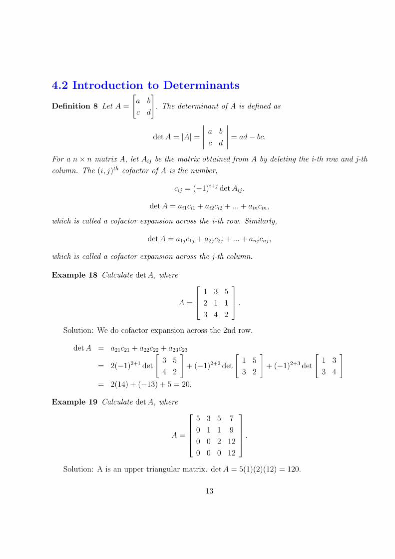
4.2 Introduction to Determinants

Definition 8 Let A =

[a b

c d

]. The determinant of A is defined as

detA = |A| =

∣∣∣∣∣ a b

c d

∣∣∣∣∣ = ad− bc.

For a n× n matrix A, let Aij be the matrix obtained from A by deleting the i-th row and j-th

column. The (i, j)th cofactor of A is the number,

cij = (−1)i+j detAij.

detA = ai1ci1 + ai2ci2 + ...+ aincin,

which is called a cofactor expansion across the i-th row. Similarly,

detA = a1jc1j + a2jc2j + ...+ anjcnj,

which is called a cofactor expansion across the j-th column.

Example 18 Calculate detA, where

A =

1 3 5

2 1 1

3 4 2

.

Solution: We do cofactor expansion across the 2nd row.

detA = a21c21 + a22c22 + a23c23

= 2(−1)2+1 det

[3 5

4 2

]+ (−1)2+2 det

[1 5

3 2

]+ (−1)2+3 det

[1 3

3 4

]= 2(14) + (−13) + 5 = 20.

Example 19 Calculate detA, where

A =

5 3 5 7

0 1 1 9

0 0 2 12

0 0 0 12

.

Solution: A is an upper triangular matrix. detA = 5(1)(2)(12) = 120.

13

4.3 Eigenvalues and Eigenvectors

Characteristic equation: det(A− λI) is called the characteristic polynomial of A and

det(A− λI) = 0

is called the characteristic equation.

Theorem 5 The solutions of the characteristic equation are the eigenvalues of A.

Example 20 Let A =

[4 5

−1 0

]. Find all eigenvalues.

Sol: det(A− λI) = λ2 − 4λ+ 5 ⇒ λ = 2± i.

Example 21 Find all eigenvalues of A, where

A =

3 2 −1

0 1 2

0 0 3

.

Solution: The characteristic polynomial is

det(A− λI) =

∣∣∣∣∣∣∣3− λ 2 −1

0 1− λ 2

0 0 3− λ

∣∣∣∣∣∣∣ = (3− λ)2(1− λ).

The solutions of the characteristic equation det(A− λI) = 0 are 3,3,1.

Algebraic and Geometric multiplicity:

• The algebraic multiplicity of an eigenvalue is equal to the number of times it is a root

of the characteristic equation.

• The geometric multiplicity of an eigenvalue is the dimension of its eigenspace.

Example 22 Let

A =

3 2 −1

0 1 2

0 0 3

.

The eigenvalue 3 has algebraic multiplicity 2 and the eigenvalue 1 has algebraic multiplicity

1. Find the corresponding eigenspaces and their geometric multiplicities.

14

Solution: When λ = 3,

A− λI = A− 3I =

0 2 −1

0 −2 2

0 0 0

R2 +R1−−−−−→

0 2 −1

0 0 1

0 0 0

R1 +R2−−−−−→

0 2 0

0 0 1

0 0 0

.

Thus (A− 3I)x⃗ = 0 has the solution

x⃗ =

x1

x2

x3

=

t

0

0

= t

1

0

0

.

The eigenspace has a basis

1

0

0

. The geometric multiplicity of the eigenvalue 3 is 1.

When λ = 1,

A− λI = A− I =

2 2 −1

0 0 2

0 0 2

R3 −R2−−−−−→

2 2 −1

0 0 2

0 0 0

R1 −1

2R2

−−−−−−→

2 2 0

0 0 2

0 0 0

.

Thus (A− I)x⃗ = 0 has the solution

x⃗ =

x1

x2

x3

=

t

−t

0

= t

1

−1

0

.

The eigenspace has a basis

1

−1

0

. The geometric multiplicity of the eigenvalue 1 is 1.

Theorem 6 (The Invertible Matrix Theorem) Let A be a square n × n matrix. Then the

following statements are equivalent.

1. A is an invertible matrix.

2. A is row equivalent to the identity matrix.

3. A has n pivot positions.

4. The equation Ax⃗ = 0⃗ has only the trivial solution.

5. The columns of A form a linearly independent set.

6. The linear transformation TA : ℜn → ℜn is 1:1.

7. The equation Ax⃗ = b⃗ has at least one solution for each b⃗ ∈ ℜn.

15

8. The columns of A span ℜn.

9. The linear transformation TA : ℜn → ℜn is onto.

10. There is an n× n matrix C such that CA = I.

11. There is an n× n matrix D such that AD = I.

12. AT is invertible.

13. The columns of A form a basis for ℜn.

14. Col A = ℜn

15. dim ColA = n

16. rank A = n

17. Nul A = {0}18. dim NulA = 0.

19. The number 0 is not an eigenvalue of A.

20. The determinant of A is not zero.

Property 4 Let λ be an eigenvalue of A with corresponding eigenvector x.

(1) For any positive integer n, λn is an eigenvalue of An with corresponding eigenvector

x.

(2) If A is invertible, then 1λis an eigenvalue of A−1 with corresponding eigenvector x.

(3) If A is invertible, then for any integer n, λn is an eigenvalue of An with corresponding

eigenvector x.

Theorem 7 If v⃗1, ..., v⃗r are eigenvectors that correspond to distinct eigenvalues λ1, . . . , λr

of an n× n matrix A, then the set {v⃗1, ..., v⃗r} is linearly independent.

Proof. We use induction.

Assume that when r = k, the set is linearly independent. When r = k + 1, if on the

contrary that the set is dependent, then

vk+1 = c1v1 + · · · ckvk.

Apply A to both sides,

λk+1vk+1 = c1λ1v1 + · · · ckλkvk.

We also have

λk+1vk+1 = c1λk+1v1 + · · · ckλk+1vk.

By subtraction,

0 = c1(λ1 − λk+1)v1 + · · · ck(λk − λk+1)vk.

Thus c1 = · · · = ck = 0, i.e., vk+1 = 0, a contradiction.

16

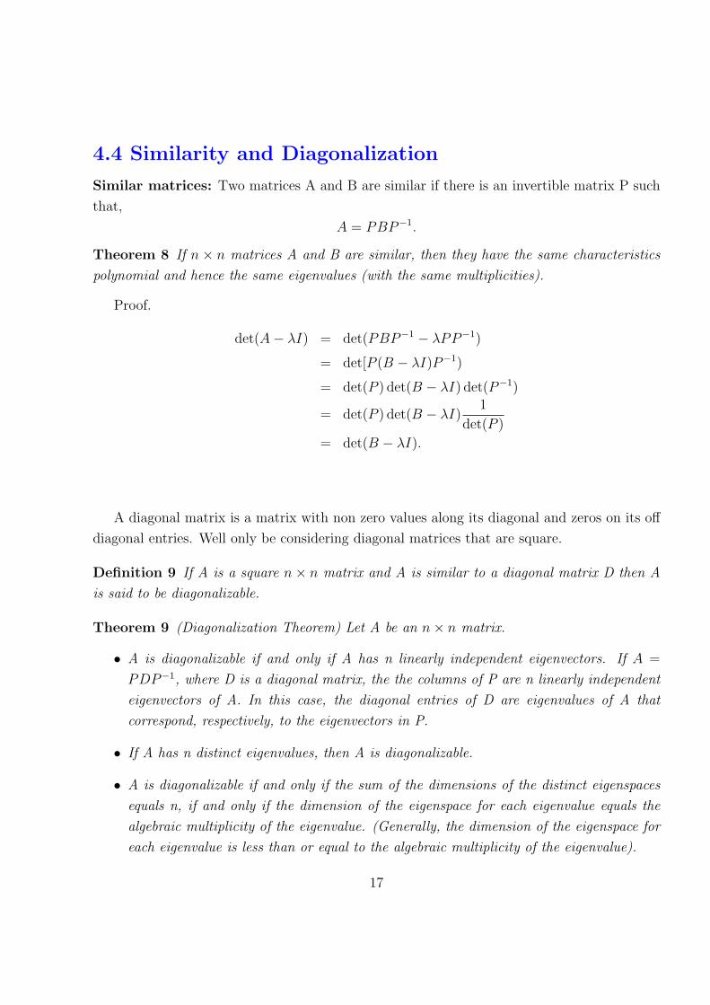
4.4 Similarity and Diagonalization

Similar matrices: Two matrices A and B are similar if there is an invertible matrix P such

that,

A = PBP−1.

Theorem 8 If n× n matrices A and B are similar, then they have the same characteristics

polynomial and hence the same eigenvalues (with the same multiplicities).

Proof.

det(A− λI) = det(PBP−1 − λPP−1)

= det[P (B − λI)P−1)

= det(P ) det(B − λI) det(P−1)

= det(P ) det(B − λI)1

det(P )

= det(B − λI).

A diagonal matrix is a matrix with non zero values along its diagonal and zeros on its off

diagonal entries. Well only be considering diagonal matrices that are square.

Definition 9 If A is a square n× n matrix and A is similar to a diagonal matrix D then A

is said to be diagonalizable.

Theorem 9 (Diagonalization Theorem) Let A be an n× n matrix.

• A is diagonalizable if and only if A has n linearly independent eigenvectors. If A =

PDP−1, where D is a diagonal matrix, the the columns of P are n linearly independent

eigenvectors of A. In this case, the diagonal entries of D are eigenvalues of A that

correspond, respectively, to the eigenvectors in P.

• If A has n distinct eigenvalues, then A is diagonalizable.

• A is diagonalizable if and only if the sum of the dimensions of the distinct eigenspaces

equals n, if and only if the dimension of the eigenspace for each eigenvalue equals the

algebraic multiplicity of the eigenvalue. (Generally, the dimension of the eigenspace for

each eigenvalue is less than or equal to the algebraic multiplicity of the eigenvalue).

17

For an n × n matrix A, if A is diagonalizable and Bk is a basis for the eigenspace cor-

responding to the eigenvalue λk, k = 1, ..., p, then the total collection of vectors in the sets

B1,..., Bp forms an eigenvector basis of Rn.

Example 23 A =

1 2 3 4

0 3 2 4

0 0 5 −1

0 0 0 7

is diagonalizable: 4 distinct eigenvalues.

B =

[3 −1

1 5

]is not diagonalizable: λ = 4, one eigenvector

[−1

1

].

Example 24 Let A =

[2 3

4 1

].

1) Find P and D such that A = PDP−1.

2) Calculate A4.

Sol: 1) det(A− λI) = (λ− 5)(λ+ 2).

When λ = 5: x⃗ = x2

[1

1

];

When λ = −2: x⃗ = x2

4

[−3

4

]. Thus

P =

[1 −3

1 4

], D =

[5 0

0 −2

]; or P =

[−3 1

4 1

], D =

[−2 0

0 5

].

2) Let P =

[1 −3

1 4

], then P−1 = 1

7

[4 3

−1 1

].

A4 ={PDP−1

}4= PD4P−1 =

[1 −3

1 4

][5 0

0 −2

]41

7

[4 3

−1 1

]

=1

7

[1 −3

1 4

][625 0

0 16

][4 3

−1 1

]=

[364 261

348 277

].

18

6.4 Linear Transformations

6.4.1 Linear Transformations

Definition 10 Let V and W be vector spaces. Then a linear transformation T from V to W

is a function with domain V and range a subset of W satisfying

1) T(u + v) = T(u) + T(v)

2) T(cu) = cT(u)

for any vectors u and v in V and scalar c.

Example 25 TA(x⃗) = Ax⃗ is linear for any matrix A.

Example 26 T : Rn → Rn by T (x⃗) = rx⃗, r a scalar. Then T is linear.

Example 27 T : Rn → Rm by T (x⃗) = Ax⃗+ b⃗, b⃗ ̸= 0⃗. Then T is non-linear.

Example 28 T : Mnn → R by T (A) = |A| = det(A). Then T is non-linear.

Example 29 Let V be the vector space of (infinitely) differentiable functions and define D to

be the function from V to V given by D(f(t)) = f ′(t). Then D is a linear transformation.

Proof. Since

D(f(t) + g(t)) = (f(t) + g(t))′ = f ′(t) + g′(t) = D(f(t)) +D(g(t)).

D(cf(t)) = (cf(t))′ = cf ′(t) = cD(f(t)).

Properties: If T is linear, then

• T (⃗0) = 0⃗.

• T (cu⃗+ dv⃗) = cT (u⃗) + dT (v⃗) for all u⃗, v⃗ in the domain of T and all scalars c, d.

Example 30 Let T : R2 → P3 by T (

[2

1

]) = 1 − x − x2, and T (

[1

2

]) = 2x + x3. Find

T (

[3

4

]).

19

6.4.2 Composition of Linear Transformations

Definition 11 Let U, V and W be vector spaces. Let T : U → V and S : V → W be two

transformations. Then the composition of S with T is S ◦ T , defined by:

(S ◦ T )(u) = S(T (u))

for any vectors u in U.

Theorem 10 If T and S are linear, then S ◦ T is linear.

Example 31 Let T : R2 → M22 and S : M22 → P3 be two linear transformations defined by:

T (

[a

b

]) =

[a b

a+ b a− b

], S(

[a b

c d

]) = a+ (b+ c)x− dx2 + (a+ c)x3.

Find S ◦ T .

6.4.3 Inverse of Linear Transformations

Definition 12 A linear transformation T : V → W is invertible if there is a linear transfor-

mation S : W → v such that

S ◦ T = IV and T ◦ S = IW .

In this case, S is called the inverse of T , and denoted by S = T−1.

Remark. T−1 is unique.

20

6.5 The Kernel and Range of a Linear Transformation

6.5.1 Kernel and range

Definition 13 Let T : V → W be a linear transformation. Kernel ker(T ) = {v ∈ V |T (v) =0⃗}, Range range(T ) = {T (v)|v ∈ V }.

Example 32 (i) ker(TA) = null(A).

(ii) If D : P3 → P2, then ker(D) = R, range(D) = P2.

(iii) If S : P1 → R is given by S(p(x)) =∫ 1

0p(x)dx, then

ker(S) = {− b

2+ bx|b ∈ R}, range(S) = R.

(iv) If T : M22 → M22 is given by T (A) = AT , then ker(T ) = {0}, range(T ) = M22.

Theorem 11 Let T : V → W be a linear transformation. Then ker(T ) is a subspace of V ,

range(T ) is a subspace of W .

6.5.2 Rank and nullity

Definition 14 Let T : V → W be a linear transformation. nullity(T ) = dim ker(T ),

rank(T ) = dim range(T ).

Example 33 Find the rank and nullity of the following:

(i) TA.

(ii) D : P3 → P2.

(iii) S : P1 → R is given by S(p(x)) =∫ 1

0p(x)dx.

(iv) T : M22 → M22 is given by T (A) = AT .

Rank Theorem: Let T : V → W be a linear transformation. Then

nullity(T ) + rank(T ) = dimV.

Proof. Let dimV = n, and let {v1, · · · , vk} be a basis for ker(T ). Then we can extend it

to a basis of V : {v1, · · · , vk, vk+1, · · · vn}. We only need to prove that {T (vk+1), · · ·T (vn)} is

a basis for range(T ).

21


T (

[a

b

]) =

[a b

a+ b a− b

], S(

[a b

c d

]) = a− b+ (b+ c)x+ (a− d)x2 + (a+ c)x3.

Find rank(T ), rank(S), nullity(T ), nullity(S).

6.5.3 One-to-One and Onto

Definition 15 Let T : V → W be a linear transformation. If T maps distinct vectors in V

to distinct vectors in W , then T is called one-to-one. If range(T ) = W , then T is called onto.

Theorem 12 Let TA : Rn → Rm be a linear transformation with standard matrix A. Then,

1. TA is onto if and only if the columns of A span Rm.

2. TA is 1:1 if and only if the columns of A are linearly independent.

3. TA is 1:1 if and only if Ax⃗ = TA(x⃗) = 0 has only the trivial solution.

Example 35 Let A =

[1 0 9

0 3 7

]. Is TA : R3 → R2 ONTO, 1:1?

Sol: TA is ONTO, since the columns of A span ℜ2. TA is not 1:1, since the columns of A

are linearly dependent.

Example 36 Let T : R2 → R3 be given by

T (x1, x2) = (x1 − 2x2,−x1 + 3x2, 3x1 − 2x2) =

1 −2

−1 3

3 −2

[x1

x2

].

Is T ONTO, 1:1?

Sol: T is not ONTO, since A has at most two pivots, the columns of A can not span R3.

TA is 1:1, since the columns of A are linearly independent.

Theorem 13 A linear transformation T : V → W is one-to-one iff ker(T ) = {0}.

Proof. If T (u) = T (v), then T (u− v) = 0.

Theorem 14 Let dimV = dimW . A linear transformation T : V → W is one-to-one if and

only if it is onto.

22

Example 37 Let T : R2 → P1 be defined by:

T (

[a

b

]) = a− b+ (b+ a)x.

Show that T is onto and one-to-one.

Theorem 15 A linear transformation T : V → W is invertible if and only if it is one-to-one

and onto.

6.5.3 Isomorphism of Vector Spaces

Definition 16 A linear transformation T : V → W is isomorphism if it is one-to-one and

onto. Then we say that V is isomorphic to W and we write V ∼= W .

Example 38 Show that Rn+1 and Pn are isomorphic.

Proof. Let T (ej) = xj−1.

Theorem 16 Let dimV < ∞, dimW < ∞. Then V ∼= W if and only if dimV = dimW.

Example 39 Show that M33 and P9 are NOT isomorphic.

23

6.6 The Matrix of a Linear Transformation

6.6.1 Matrix of Linear Transformation

Definition 17 Let V and W be two vector spaces with dimV = n and dimW = m. Let

B = {v1, · · · , vn} be a basis of V and C be a basis of W . Then

A = [[T (v1)]C · · · [T (vn)]C ]

is called the matrix of T with respect to bases B and C. We write A = [T ]C←B. when V = W

and B = C, we simply write [T ]C←B as [T ]B.

Theorem 17 For every v ∈ V , A[v]B = [T (v)]C.

Proof. Define isomorphisms N : V → Rn and M : W → Rm as follows:

N(v) = [v]B, M(w) = [w]C .

Then N(vi) = ei. Thus

(M ◦ T ◦N)([v]B) = [T (v)]C .

Example 40 Let T : R3 → R2 be given by

T (

x

y

z

) = [x+ 2y

y − 3z

].

Let B = {e1, e2, e3} and C = {e1, e2}.(i) Find the matrix of T with respect to bases B and C.

(ii) Verify A[v]B = [T (v)]C for

1

2

3

.Example 41 Let T : P2 → P2 be given by

T (p(x)) = p(2 + x).

Let B = {1, x, x2}.(i) Find the matrix [T ]B.

(ii) Use (i) to calculate T (1− x− x2).

24

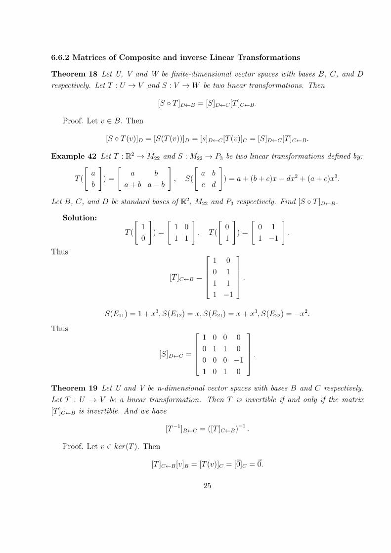
6.6.2 Matrices of Composite and inverse Linear Transformations

Theorem 18 Let U, V and W be finite-dimensional vector spaces with bases B, C, and D

respectively. Let T : U → V and S : V → W be two linear transformations. Then

[S ◦ T ]D←B = [S]D←C [T ]C←B.

Proof. Let v ∈ B. Then

[S ◦ T (v)]D = [S(T (v))]D = [s]D←C [T (v)]C = [S]D←C [T ]C←B.


T (

[a

b

]) =

[a b

a+ b a− b

], S(

[a b

c d

]) = a+ (b+ c)x− dx2 + (a+ c)x3.

Let B, C, and D be standard bases of R2, M22 and P3 respectively. Find [S ◦ T ]D←B.

Solution:

T (

[1

0

]) =

[1 0

1 1

], T (

[0

1

]) =

[0 1

1 −1

].

Thus

[T ]C←B =

1 0

0 1

1 1

1 −1

.

S(E11) = 1 + x3, S(E12) = x, S(E21) = x+ x3, S(E22) = −x2.

Thus

[S]D←C =

1 0 0 0

0 1 1 0

0 0 0 −1

1 0 1 0

.

Theorem 19 Let U and V be n-dimensional vector spaces with bases B and C respectively.

Let T : U → V be a linear transformation. Then T is invertible if and only if the matrix

[T ]C←B is invertible. And we have

[T−1]B←C = ([T ]C←B)−1 .

Proof. Let v ∈ ker(T ). Then

[T ]C←B[v]B = [T (v)]C = [⃗0]C = 0⃗.

25

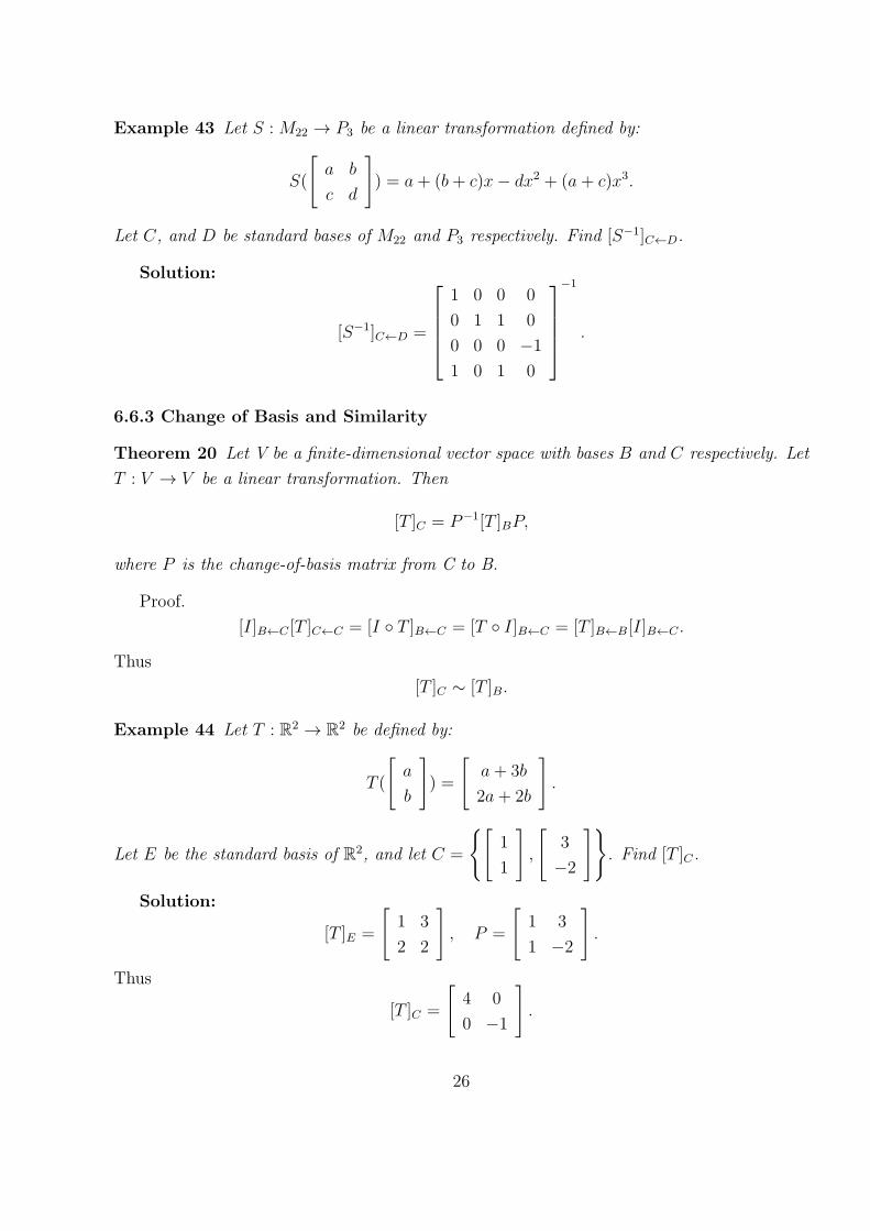
Example 43 Let S : M22 → P3 be a linear transformation defined by:

S(

[a b

c d

]) = a+ (b+ c)x− dx2 + (a+ c)x3.

Let C, and D be standard bases of M22 and P3 respectively. Find [S−1]C←D.

Solution:

[S−1]C←D =

1 0 0 0

0 1 1 0

0 0 0 −1

1 0 1 0

−1

.

6.6.3 Change of Basis and Similarity

Theorem 20 Let V be a finite-dimensional vector space with bases B and C respectively. Let

T : V → V be a linear transformation. Then

[T ]C = P−1[T ]BP,

where P is the change-of-basis matrix from C to B.

Proof.

[I]B←C [T ]C←C = [I ◦ T ]B←C = [T ◦ I]B←C = [T ]B←B[I]B←C .

Thus

[T ]C ∼ [T ]B.

Example 44 Let T : R2 → R2 be defined by:

T (

[a

b

]) =

[a+ 3b

2a+ 2b

].

Let E be the standard basis of R2, and let C =

{[1

1

],

[3

−2

]}. Find [T ]C.

Solution:

[T ]E =

[1 3

2 2

], P =

[1 3

1 −2

].

Thus

[T ]C =

[4 0

0 −1

].

26

Definition 18 Let V be a finite-dimensional vector space and let T : V → V be a linear

transformation. If there is a basis C of V such that [T ]C is a diagonal matrix, then T is called

diagonalizable.

Example 45 Let T : P2 → P2 be given by

T (p(x)) = p(2x− 1).

Let E be the standard basis of R2, and let B = {1 + x, 1− x, x2}.(i) Find the matrix [T ]B.

(ii) Show that T is diagonalizable by finding a basis C such that [T ]C is a diagonal matrix.

Solution:

(i) [T ]E =

1 −1 1

0 2 −4

0 0 4

, PE←B =

1 1 0

1 −1 0

0 0 1

. Thus

[T ]B =

1 0 −32

−1 2 52

0 0 4

.

(ii) C = {1,−1 + x, 1− 2x+ x2}.

27

6.7 An Application: Homogeneous Linear Differential

Equation

6.7.1 First Order Homogeneous Linear Differential Equation

First Order Homogeneous Linear Differential Equation:

y′(t) + ay(t) = 0,

where a is a constant.

Theorem 21 Let S = {y|y′ + ay = 0}. Then(i) S is a subspace of F .

(ii) {e−at} is a basis of S, dimS = 1.

Proof. Let x(t) be a general solution. Then [x(t)eat]′ = 0.

Example 46 A bacteria culture growth at a rate proportional to its size. After 2 hours there

are 40 bacteria and after 4 hours the count is 120. Find an expression for the population after

t hours.

Solution: We measure the time t in hours. Let P (t) be the population at t hours, then

we havedP

dt= kP.

The solution of the equation is

P (t) = P (0)ekt.

Note that P (2) = 40 and P (4) = 120, we obtain

40 = P (0)e2k, 120 = P (0)e4k.

These imply that

P (0) =40

3and

e2k = 3, or k = ln 3/2.

We thus have

P (t) =40

33t/2 =

40

3

√3t=

40

3e(ln 3/2)t.

28

Example 47 The half-life of Sodium-24 is 15 hours. Suppose you have 100 grams of Sodium-

24. How many grams remaining after 27 minutes (keep three decimals)?

Solution: Assume m(t) be the amount after t hours. Then

m(t) = m(0)(1

2)t/H ,

where m(0) = 100, H = 15 hours. Note that 27 minutes = 27/60=0.45 hours. Thus

m(0.45) = 100(1

2)0.45/15 = 100(

1

2)0.03 = 97.942g.

6.7.2 Second Order Homogeneous Linear Differential Equation

Second Order Homogeneous Linear Differential Equation:

y′′(t) + ay′(t) + by(t) = 0,

where a and b are constants.

Theorem 22 Let S = {y|y′′(t) + ay′(t) + by(t) = 0}, and let λ1 and λ2 be the two solutions

of the characteristic equation λ2 + aλ+ b = 0. Then

(i) S is a subspace of F .

(ii) If λ1 ̸= λ2, then {eλ1t, eλ2t} is a basis of S, dimS = 2.

(iii) If λ1 = λ2, then {eλ1t, teλ1t} is a basis of S, dimS = 2.

Proof. Omitted.

Example 48 Find the solution spaces of y′′(t)−y′(t)−12y(t) = 0 and y′′(t)−6y′(t)+9y(t) = 0.

6.7.3 Linear Codes

For the purposes of coding, we will be working with linear algebra.

Let Znp be the set of vectors of length n (n entries) such that each entry is an integer

between 0 and p1 (inclusive). Only scalars are 0, 1,..., p− 1. The addition is

a+ b = c(mod p).

For example, 3 + 4 = 2(mod 5).

Definition 19 A linear code C is a subspace of Znp . If dimC = k, then C is called (n, k)

code.

29

Example 49 Let C1 =

0

0

0

0

,

1

1

1

1

,

0

0

1

1

,

1

1

0

0

,

C2 =

0

0

0

0

,

1

1

1

1

,

0

1

1

1

,

1

1

0

0

.

Show that C1 is a linear code, but C2 is not a linear code.

30

5.1 Orthogonality in Rn

5.1.1 Review

Definition 20 Let u⃗, v⃗ be two vectors in Rn. i.e.

u⃗ =

u1

u2

...

un

, v⃗ =

v1

v2...

vn

.

The number u⃗T v⃗ = u1v1 + u2v2 + ...+ unvn is called the inner product or dot product of u⃗ and

v⃗ and is denoted as u⃗ · v⃗.

Definition 21 The length or norm of a vector v⃗ =

v1

v2...

vn

is a defined by,

||v⃗|| =√v⃗ · v⃗ =

√v21 + ...+ v2n.

If c is a scalar, then ||cv⃗|| = |c|||v⃗||.Normalization: When the length of a vector is 1 that vector is called a unit vector. Given

any vector v⃗ we can change it into a unit vector:

v⃗

||v⃗||

is a unit vector in the direction of v⃗;

− v⃗

||v⃗||is a unit vector in the opposite direction of v⃗.

This process of constructing a unit vector in the direction of a given vector v⃗ is called

normalizing v⃗.

Definition 22 Let u⃗, v⃗ be two vectors in Rn. The distance between u⃗, v⃗ is the length of the

vector u⃗− v⃗:

dist(u⃗, v⃗) = ||u⃗− v⃗||.

31

Angle between two vectors: Let u⃗, v⃗ be two vectors, and let θ ≤ π be the angle between

them. Then

cos θ =u⃗ · v⃗

||u⃗||||v⃗||.

5.1.2 Orthogonal Set

Definition 23 (Orthogonality) Let u⃗, v⃗ be two vectors in Rn. They are said to be orthogonal

if u⃗ · v⃗ = 0.

Theorem 23 (The Pythagorean Theorem) Two vectors u⃗, v⃗ are orthogonal if and only if

||u⃗+ v⃗||2 = ||u⃗||2 + ||v⃗||2.

Definition 24 If each pair of distinct vectors in a set is orthogonal then the set is called an

orthogonal set.

Example 50 Is the set

v⃗1 =

0

1

−2

1

, v⃗2 =

0

0

1

2

, v⃗3 =

0

−5

−2

1

an orthogonal set?

Sol: We need to check

v⃗1 · v⃗2 = 0 + 0 + (−2) + 2 = 0

v⃗1 · v⃗3 = 0 + (−5) + 4 + 1 = 0

v⃗2 · v⃗3 = 0 + 0 + (−2) + 2 = 0.

Thus v⃗1⊥v⃗2, v⃗1⊥v⃗3, v⃗2⊥v⃗3, the set is orthogonal.

Theorem 24 If a set of non-zero vectors is orthogonal, then the set is linearly independent.

Definition 25 (Orthogonal Basis) If S = {v⃗1, v⃗2, ..., v⃗m} is an orthogonal set of non-zero

vectors, then it is called an orthogonal basis for the subspace W = Span{v⃗1, v⃗2, ..., v⃗m}.

Example 51 Let v1 =

1

−2

1

, v⃗2 =

0

1

2

, v⃗3 =

−5

−2

1

.Show that {v⃗1, v⃗2, v⃗3} is an orthogonal basis for R3.

32

Proof.

v⃗1 · v⃗2 = 0 + (−2) + 2 = 0

v⃗1 · v⃗3 = (−5) + 4 + 1 = 0

v⃗2 · v⃗3 = 0 + (−2) + 2 = 0.

Thus v⃗1⊥v⃗2, v⃗1⊥v⃗3, v⃗2⊥v⃗3. The set {v⃗1, v⃗2, v⃗3} is orthogonal of non-zero vectors, so they are

linearly independent. Three such vectors automatically form a basis for R3.

Theorem 25 If y⃗ is a vector in W = Span{v⃗1, v⃗2, ..., v⃗m}, where S = {v⃗1, v⃗2, ..., v⃗m} is an

orthogonal set of non-zero vectors, then it may be written uniquely as a linear combination of

the vectors in S,

y⃗ = c1v⃗1 + c2v⃗2 + ...+ cmv⃗m, ck =y⃗ · v⃗kv⃗k · v⃗k

, k = 1, ...,m.

Proof.

y⃗ · v⃗1 = (c1v⃗1 + c2v⃗2 + ...+ cmv⃗m) · v⃗1= c1v⃗1 · v⃗1 + c2v⃗2 · v⃗1 + ...+ cmv⃗m · v⃗1= c1v⃗1 · v⃗1 + 0.

Example 52 Let v1 =

1

−2

1

, v⃗2 =

0

1

2

, v⃗3 =

−5

−2

1

, x⃗ =

3

2

1

. Represent x⃗ as a

linear combination of {v⃗1, v⃗2, v⃗3} .

5.1.2 Orthonormal Set

Definition 26 If S = {u⃗1, u⃗2, ..., u⃗m} is an orthogonal set of unit vectors, then it is called

an orthonormal set. If an orthonormal set S spans some subspace W, then S is called an

orthonormal basis for W. (S is an orthogonal set that spans W, so is linearly independent and

thus a basis for W.)

Example 53 The set {e⃗1, e⃗2, ..., e⃗n} is an orthonormal set that spans Rn, thus an orthonormal

basis for Rn, which is called the standard basis for Rn.

Theorem 26 A matrix A has orthonormal columns if and only if ATA = I.

Definition 27 An n × n matrix U is called an orthogonal matrix if its columns form an

orthonormal set.

33

Theorem 27 An n× n matrix U is an orthogonal matrix if and only if U−1 = UT .

Example 54 Show that A =

√2/6

√2/2 −2/3

4√2/6 0 1/3√2/6 −

√2/2 −2/3

is an orthogonal matrix.

Proof. It is easy to see that ATA = I. Thus A−1 = AT .

Example 55 A =

√2/6

√2/2 −2/3

4√2/6 0 1/3√2/6 −

√2/2 −2/3

has orthonormal columns.

Theorem 28 Let A be an m × n matrix with orthonormal columns, and let x⃗, y⃗ be in Rn.

Then,

1. ||Ax⃗|| = ||x⃗||.2. (Ax⃗) · (Ay⃗) = x⃗ · y⃗.3. (Ax⃗) · (Ay⃗) = 0 if and only if x⃗ · y⃗ = 0.

Proof. 1.

||Ax⃗||2 = (Ax⃗)T (Ax⃗) = x⃗TATAx⃗ = x⃗T Ix⃗ = x⃗T x⃗ = ||x⃗||2.

2.

(Ax⃗) · (Ay⃗) = (Ax⃗)T (Ay⃗) = x⃗TATAy⃗ = x⃗T Iy⃗ = x⃗T y⃗.

Property 5 Let A be an orthogonal matrix. Then

(i) A−1 is orthogonal.

(ii) det(A) = ±1.

(iii) If λ is an eigenvalue of A, then λ = ±1.

(iv) If A and B are orthogonal n× n matrices, then so is AB.

5.2 Orthogonal Complements and Orthogonal Projec-

tions

5.2.1 Orthogonal Complements

Definition 28 (Orthogonal Complement) Let W be a plane and L a line intersecting W. At

the point of intersection of the line L to the plane W, L is orthogonal to W. We call L the

orthogonal complement of W and denote it by L = W⊥. Similarly, we may think of W as

34

being perpendicular to L and so may be called the orthogonal complement of L and is denoted

by, W = L⊥.

Properties of Orthogonal Complement:

• A vector x⃗ is in W⊥ if and only if x⃗ is orthogonal to every vector in a set that spans W.

• W⊥ is a subspace.

• W∩

W⊥ = {0}.

• If W = span{w1, ..., wk}, then v ∈ W⊥ if and only if v · wi = 0 for all i.

• (RowA)⊥ = NulA, (ColA)⊥ = NulAT .

Example 56 Let

W = span

−1

2

1

,

3

1

1

, x⃗ =

1

4

−7

.

1) Show that x⃗ ∈ W⊥.

2) Find other vectors in W⊥.

Solution: 1) −1

2

1

· x⃗ = 0,

3

1

1

· x⃗ = 0.

2) Let x⃗ =

x1

x2

x3

∈ W⊥. Then

−1

2

1

· x⃗ = 0,

3

1

1

· x⃗ = 0 ⇒

Ax⃗ = 0, A =

[−1 2 1

3 1 1

]∼

[−4 1 0

0 7 4

].

The solution of this is: x1 = 1/4x2, x3 = −7/4x2, i.e.,

x⃗ = 1/4x2

1

4

−7

.

35

5.2.2 Orthogonal Projections

Given two vectors v⃗ and x⃗, we would like to write v⃗ as a linear combination of two orthogonal

vectors: one vector in the direction of the vector x⃗ and another vector, y⃗, orthogonal to x⃗. So,

v⃗ = αx⃗+ y⃗,⇒ α =v⃗ · x⃗x⃗ · x⃗

,⇒ y⃗ = v⃗ − v⃗ · x⃗x⃗ · x⃗

x⃗.

Definition 29

projx⃗v⃗ =v⃗ · x⃗x⃗ · x⃗

x⃗

is called the orthogonal projection of v⃗ onto x⃗ and

perpx⃗v⃗ = v⃗ − v⃗ · x⃗x⃗ · x⃗

x⃗

is the component of v⃗ orthogonal to x⃗. If W = Span{v⃗1, v⃗2, ..., v⃗m}, where S = {v⃗1, v⃗2, ..., v⃗m}is an orthogonal set of non-zero vectors, then the orthogonal projection of y⃗ onto W is defined

as

projW y⃗ = c1v⃗1 + c2v⃗2 + ...+ cmv⃗m, ck =y⃗ · v⃗kv⃗k · v⃗k

, k = 1, ...,m.

The complement of y⃗ orthogonal to W is

perpW y⃗ = y⃗ − projW y⃗.

Example 57 Let v⃗ =

[1

−2

], x⃗ =

[1

2

]1) Find the orthogonal projection of v⃗ onto x⃗.

2) Write v⃗ as the sum of two vectors, one in Span{x⃗} and one orthogonal to x⃗.

3) Find the distance from v⃗ to the line through x⃗ and the origin (i.e., L = Span{x⃗}).

Sol: 1)

ˆ⃗v =v⃗ · x⃗x⃗ · x⃗

x⃗ =−3

5

[1

2

]=

[−0.6

−1.2

].

2) The component of v⃗ orthogonal to x⃗ is

v⃗ − ˆ⃗v =

[1.6

3.2

].

Thus

v⃗ =

[−0.6

−1.2

]+

[1.6

3.2

].

36

3) The distance is

||v⃗ − ˆ⃗v|| = ||

[1.6

3.2

]|| =

√1.62 + 3.22 =

√12.8.

5.2.3 The orthogonal Decomposition Theorem

Theorem 29 Let W be a subspace of Rn with orthogonal basis {v⃗1, v⃗2, ..., v⃗m}. Then each y⃗

in Rn can be written uniquely in the form

y⃗ = ˆ⃗y + z⃗, ˆ⃗y ∈ W, z⃗ ∈ W⊥,

whereˆ⃗y =

y⃗ · v⃗1v⃗1 · v⃗1

v⃗1 + · · ·+ y⃗ · v⃗mv⃗m · v⃗m

v⃗m,

z⃗ = y⃗ − ˆ⃗y.

Example 58 Let y⃗ =

1

1

1

1

, v⃗1 =

0

1

−2

1

, v⃗2 =

0

0

1

2

, v⃗3 =

0

−5

−2

1

. LetW = Span{v⃗1, v⃗2, v⃗3}.

Find projW y⃗.

Sol: Since

v⃗1 · v⃗2 = 0 + 0 + (−2) + 2 = 0

v⃗1 · v⃗3 = 0 + (−5) + 4 + 1 = 0

v⃗2 · v⃗3 = 0 + 0 + (−2) + 2 = 0.

Thus v⃗1⊥v⃗2, v⃗1⊥v⃗3, v⃗2⊥v⃗3, the set {v⃗1, v⃗2, v⃗3} is orthogonal basis of W.

projW y⃗ = ˆ⃗y =y⃗ · v⃗1v⃗1 · v⃗1

v⃗1 +y⃗ · v⃗2v⃗2 · v⃗2

v⃗2 +y⃗ · v⃗3v⃗3 · v⃗3

v⃗3 = 0

0

1

−2

1

+3

5

0

0

1

2

+−6

5

0

−5

−2

1

=

0

6

3

0

.

Property: If we have an orthogonal basis {v⃗1, v⃗2, ..., v⃗m} for W and if y⃗ ∈ W , then projW y⃗ =

y⃗.

37

Proof. Since y⃗ ∈ W ,

y⃗ = d1v⃗1 + d2v⃗2 + ...+ dmv⃗m. ⇒

y⃗ · v⃗1 = d1v⃗1 · v⃗1, ..., y⃗ · v⃗m = dmv⃗m · v⃗m.

Thus

projW y⃗ =y⃗ · v⃗1v⃗1 · v⃗1

v⃗1 + · · ·+ y⃗ · v⃗mv⃗m · v⃗m

v⃗m

=d1v⃗1 · v⃗1v⃗1 · v⃗1

v⃗1 + · · ·+ dmv⃗m · v⃗mv⃗m · v⃗m

v⃗m

= d1v⃗1 + d2v⃗2 + ...+ dmv⃗m

= y⃗.

Theorem 30 Let W be a subspace of Rn with orthonormal basis {u⃗1, u⃗2, ..., u⃗m}. Then for

each y⃗ in Rn,ˆ⃗y = projW y⃗ = (y⃗ · u⃗1)u⃗1 + · · ·+ (y⃗ · u⃗m)u⃗m.

If U = [u⃗1 u⃗2 · · · u⃗m] then

projW y⃗ = UUT y⃗.


1

1

1

, u⃗1 =

2/3

1/3

2/3

, u⃗2 =

−2/3

2/3

1/3

. Let W = Span{u⃗1, u⃗2}. Find

projW y⃗.

Note that u⃗1 · u⃗2 = 0, ||u⃗1|| = ||u⃗2|| = 1, {u⃗1, u⃗2} is orthonomal basis of W.

projW y⃗ = UUT y⃗ =

2/3 −2/3

1/3 2/3

2/3 1/3

2/3 −2/3

1/3 2/3

2/3 1/3

T 1

1

1

=

8/9

7/9

11/9

.

Theorem 31 (The Best Approximation Theorem) Let W be a subspace of Rn, y⃗ in Rn andˆ⃗y be the orthogonal projection of y⃗ onto W. Then ˆ⃗y is the closest point in W to y⃗ in the sense

that

||y⃗ − ˆ⃗y|| < ||y⃗ − v⃗||

for all v⃗ ∈ W distinct from ˆ⃗y.


3

−1

1

13

, v⃗1 =

1

−2

−1

2

, v⃗2 =

−4

1

0

3

. Let W = Span{v⃗1, v⃗2}. Find

the distance from y⃗ to W.

38

Sol: The closest point in W to y⃗ is projW y⃗. So the distance is ||y⃗ − projW y⃗||. Note that

v⃗1 · v⃗2 = 0, {v⃗1, v⃗2} is orthogonal basis of W,

projW y⃗ =y⃗ · v⃗1v⃗1 · v⃗1

v⃗1 +y⃗ · v⃗2v⃗2 · v⃗2

v⃗2 =

−1

−5

−3

9

,⇒ y⃗ − projW y⃗ =

4

4

4

4

,⇒ ||y⃗ − projW y⃗|| = 8.

Theorem 32 If W is a subspace of Rn, then

dimW + dimW⊥ = n.

Proof. (1) A basis of W and a basis of W⊥ form a linearly independent set; (2) By

decomposition theorem, any vector in Rn can be written as a linear combination of the set.

39

5.3 The Gram-Schmidt Process and the QR Factorization

5.3.1 The Gram-Schmidt Process (Algorithm)

Let S = {X1, X2, · · · , Xk} be a set of vectors, and let

F1 = X1

F2 = X2 −X2 · F1

||F1||2F1

· · ·Fk = Xk −

Xk · F1

||F1||2F1 −

Xk · F2

||F2||2F2 − · · · − −Xk · Fk−1

||Fk−1||2Fk−1.

Then {F1, F2, · · · , Fk} is an orthogonal set.

Example 61 Consider the following independent set S = {X1, X2, X3} of vectors from R4:

X1 =

1

1

1

1

, X2 =

6

0

0

2

, X3 =

−1

−1

2

4

.

Use the Gram-Schmidt algorithm to convert the set S = {X1, X2, X3} into an orthogonal set

B = {F1, F2, F3}.

Solution: Let F1 = X1 =

1

1

1

1

. Then

F2 = X2 −X2 · F1

||F1||2F1 =

6

0

0

2

− 8

4

1

1

1

1

=

4

−2

−2

0

.

F3 = X3 −X3 · F1

||F1||2F1 −

X3 · F2

||F2||2F2 =

−1

−1

2

4

− 4

4

1

1

1

1

− −6

24

4

−2

−2

0

=

−1

−2.5

0.5

3

.

40

5.3.2 The QR Factorization

By the Gram-Schmidt Process (Algorithm), we get the following QR Factorization:

Theorem 33 If A is m× n matrix with linearly independent columns, then

A = QR,

where Q is an m× n matrix with orthonormal columns, and R is an upper triangular matrix.

Proof. Let {X1, X2, · · · , Xk} be the columns of A. Then there exists orthonormal set

{F1, F2, · · · , Fk} such that

X1 = c11F1

X2 = c21F1 + c22F2

· · ·Xk = ck1F1 + ck2F2 + ckkFk.

Remark. cij = Xi · Fj.

Example 62 1 0 −3

0 2 −1

1 0 1

1 3 5

=

1√3

− 1√10

− 3√23

0 2√10

− 3√23

1√3

− 1√10

1√23

1√3

2√10

2√23

√3

√3

√3

0√10

√10

0 0√23

.

41

5.4 Orthogonal Diagonalization of Symmetric Matrix

Definition 30 A square matrix A is orthogonally diagonalizable if there exist an orthogonal

matrix Q and a diagonal matrix D such that

QTAQ = D.

Conditions under which a matrix is orthogonally diagonalizable:

Spectral Theorem. Let A be a real square matrix. Then A is orthogonally diagonalizable

if and only if A is symmetric.

Property 6 Let A be symmetric.

(i) If A is real, then all eigenvalues are real.

(ii) Any two eigenvectors corresponding to distinct eigenvalues are orthogonal.

Proof. Using x · y = xTy.

Method to orthogonally diagonalize a symmetric matrix: Columns of Q consist of

orthonormal bases of all eigenspaces.

Example 63 Orthogonally diagonalize the matrix A =

2 1 1

1 2 1

1 1 2

Solution: Step 1: Find all eigenvalues: The characteristic polynomial is−λ3+6λ2−9λ+4.

So λ = 1, 4.

Step 2: Find bases to each eigenspace:

Basis for E1:

−1

0

1

,

−1

1

0

.

Basis for E4:

1

1

1

.

Step 3: Find orthogonal bases to each eigenspace using Gram-Schmidt Process:

42

For E1:

−1

0

1

,

−1/2

1

−1/2

.

Basis for E4:

1

1

1

.

Step 4: Find orthonormal bases to each eigenspace:

For E1:

−1/

√2

0

1/√2

,

−1/√6

2/√6

−1/√6

.

Basis for E4:

1/

√3

1/√3

1/√3

.

Step 5: Construct Q and D:

Q =

−1/√2 −1/

√6 1/

√3

0 2/√6 1/

√3

−1/√2 −1/

√6 1/

√3

, D =

1 0 0

0 1 0

0 0 4

.

43

5.5 An Application: Quadratic Forms

5.5.1 Quadratic Forms

Definition 31 A quadric form in n variables is a function f : Rn → R of the form

f(x) = xTAx, x ∈ Rn,

where A is a symmetric n× n matrix. We call A the matrix associated with f .

• Quadric form in 2 variables: ax2 + by2 + cxy.

• Quadric form in 3 variables: ax2 + by2 + cz2 + dxy + exz + fyz.

Example 64 Find the matrix associated with the quadratic form

f(x1, x2, x3) = 2x21 + 3x2

2 − 1x33 − 8x1x2 + 10x2x3.

Solution: The coefficients of the squared terms x2i go on the diagonal as aii of A; the

coefficients of the cross-product terms xixj are split into half between aij and aji. Thus

A =

2 −4 0

−4 3 5

0 5 −1

.

The Principle Axes Theorem:

Every quadratic form can be diagonalized.

Specifically, if A is the n× n symmetric matrix associated with the quadratic form xTAx,

and if Q is an orthogonal matrix such that QTAQ = D is an diagonal matrix, then the change

of variable

x = Qy

transforms xTAx into the quadratic form yTDy:

xTAx = yTDy = λ1y21 + λ2y

22 + · · ·+ λny

2n,

where λ1, λ2, · · · , λn are the eigenvalues of A, y =

y1

...

yn

. The process is called diago-

nalizing a quadratic form.

44

Example 65 Find a change of variable that transforms the quadratic form associated with

the matrix A =

[5 2

2 8

]as a quadratic form with no cross-product terms. Test the result

with x =

[2

1

].

Solution: The quadratic form is f(x) = 5x21 + 8x2

2 + 4x1x2.

Step 1: Find all eigenvalues: λ = 9, 4.

Step 2: Find corresponding unit eigenvectors:

When λ = 9: q1 =

[1/√5

2/√5

].

When λ = 4: q2 =

[2/√5

−1/√5

].

Step 3: Construct Q and D:

Q =

[1/√5 2/

√5

2/√5 −1/

√5

], D =

[9 0

0 4

].

Step 4: Let x = Qy, then

f(y) = f(y1, y2) = 9y21 + 4y22.

Step 5: When x =

[2

1

], y = QTx =

[4/√5

3/√5

].

f(x) = 36, f(y) = 36.

Definition 32 A quadratic form f(x) = xTAx ( and also a symmetric matrix A) is classified

as one of the following:

1. positive definite if f(x) > 0 for all x ̸= 0;

2. positive semidefinite if f(x) ≥ 0 for all x;

3. negative definite if f(x) < 0 for all x ̸= 0;

4. negative definite if f(x) ≤ 0 for all x;

5. indefinite if f(x) takes on both positive and negative values.

Theorem 34 A quadratic form f(x) = xTAx ( and also a symmetric matrix A) is

1. positive definite if and only if the eigenvalues of A are positive;

45

2. positive semidefinite if and only if the eigenvalues of A are nonnegative;

3. negative definite if and only if the eigenvalues of A are negative;

4. negative definite if and only if the eigenvalues of A are nonpositive;

5. indefinite if and only if the eigenvalues of A are both positive and negative.

Proof. Let x = Qy.

Example 66 Classify f(x, y, z) = y2+2xy+4xz+2yz as positive definite, negative definite,

indefinite, or none of them.

Solution: The eigenvalues of A are -2, 0, 3. Thus it is indefinite.

5.5.2 Constrained Optimization Problem

Theorem 35 Let f(x) = xTAx be a quadratic form. Let λ1 ≥ λ2 ≥ · · · ≥ λn be the eigenval-

ues of A. Then the following are true subject to the constraint ||x|| = 1:

1. λ1 ≥ f(x) ≥ λn.

2. The maximum value of f(x) is λ1, and it occurs when x is an eigenvector corresponding

to λ1.

3. The minimum value of f(x) is λn, and it occurs when x is an eigenvector corresponding

to λn.

Proof. Using x = Qy. Then 1 = xTx = yTy.

Example 67 Find the max and min of f(x, y) = 5x2 +2y2 +4xy subject to x2 + y2 = 1, and

determine values of x and y for which each of these occurs.

Solution: max f is 6, when (x, y) = (2/√5, 1/

√5); min f is 1, when (x, y) = (1/

√5,−2/

√5).

46

5.5.3 Graphing quadratic equations

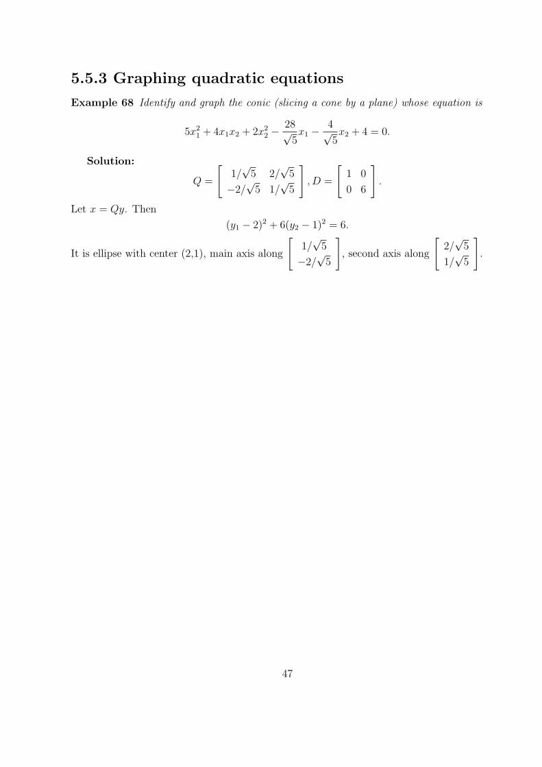
Example 68 Identify and graph the conic (slicing a cone by a plane) whose equation is

5x21 + 4x1x2 + 2x2

2 −28√5x1 −

4√5x2 + 4 = 0.

Solution:

Q =

[1/√5 2/

√5

−2/√5 1/

√5

], D =

[1 0

0 6

].

Let x = Qy. Then

(y1 − 2)2 + 6(y2 − 1)2 = 6.

It is ellipse with center (2,1), main axis along

[1/√5

−2/√5

], second axis along

[2/√5

1/√5

].

47

7.1 Inner Product Spaces

7.1.1 Inner Product

Definition 33 Suppose u, v, and w are vectors in a vector space V and c is any scalar. An

inner product on the vector space V is a function that associates with each pair of vectors in

V, say u and v, a real number denoted by < u, v > that satisfies the following axioms.

(a) < u, v >=< v, u >,

(b) < u, v + w >=< u, v > + < u,w >,

(c) < cu, v >= c < u, v >,

(d) < u, u >≥ 0, and < u, u >= 0 if and only if u = 0.

A vector space along with an inner product is called an inner product space.

Example 69 Let u⃗, v⃗ be two vectors in Rn. i.e.

u⃗ =

u1

u2

...

un

, v⃗ =

v1

v2...

vn

.

The following are inner products:

• Dot product: < u, v >= u⃗ · v⃗ = u⃗T v⃗ = u1v1 + u2v2 + ...+ unvn.

• Weighted dot product: < u, v >= w1u1v1 +w2u2v2 + ...+wnunvn, where w1, · · · , wn are

positive scales.

Example 70 • Let A be symmetric, positive definite matrix. < u, v >= uTAv defines an

inner product.

• < A,B >= trace(ATB) defines an inner product on M22.

• < f, g >=∫ b

af(x)g(x)dx defines an inner product on C[a, b].

• < a1 + b1x+ c1x2, a2 + b2x+ c2x

2 >= a1a2 + b1b2 + c1c2 defines an inner product on P2.

Property 7 Suppose u, v, and w are vectors in an inner product vector space V and c is any

scalar.

48

(a) < u+ v, w >=< u,w > + < u,w >,

(b) < u, cv >= c < u, v >,

(c) < u, 0 >=< 0, v >= 0.

7.1.2 Length, Distance and Orthogonality

Definition 34 Suppose u, v, and w are vectors in an inner product vector space V and c is

any scalar.

1. The length or norm of v is ||v|| = √< v, v >.

2. The distance between u and v is d(u, v) = ||u− v||.

3. u and v are orthogonal if < u, v >= 0.

A vector of length 1 is called a unit vector.

Example 71 • Consider the inner product < f, g >=∫ 1

0f(x)g(x)dx defined on C[a, b].

Given f(x) = 1 + 3x, g(x) = 1− 3x. Calculate ||f ||, d(f, g), and < f, g >.

• Consider the inner product < a1 + b1x+ c1x2, a2 + b2x+ c2x

2 >= a1a2 + b1b2 + c1c2 on

P2. Given f(x) = 1 + 3x, g(x) = 1− 3x. Calculate ||f ||, d(f, g), and < f, g >.

Pythagoras’ Theorem. Let u, v be vectors in an inner product vector space V. Then u and

v are orthogonal if and only if ||u+ v||2 = ||u||2 + ||v||2.

Proof. ||u+ v||2 =< u+ v, u+ v >.

7.1.3 Orthogonal Projections and the Gram-Schmidt Pro-

cess

Example 72 Apply the Gram-Schmidt Process to the basis {1, x, x2, x3} of P3 to find a basis

that is orthogonal with respect to the inner product < f, g >=∫ 1

−1 f(x)g(x)dx.

Solution: {1, x, x2 − 13, x3 − 3

5x}. Remark. They are called Legendre Polynomials. If we

divide them by their lengths, then they are called normalized Legendre Polynomials.

49

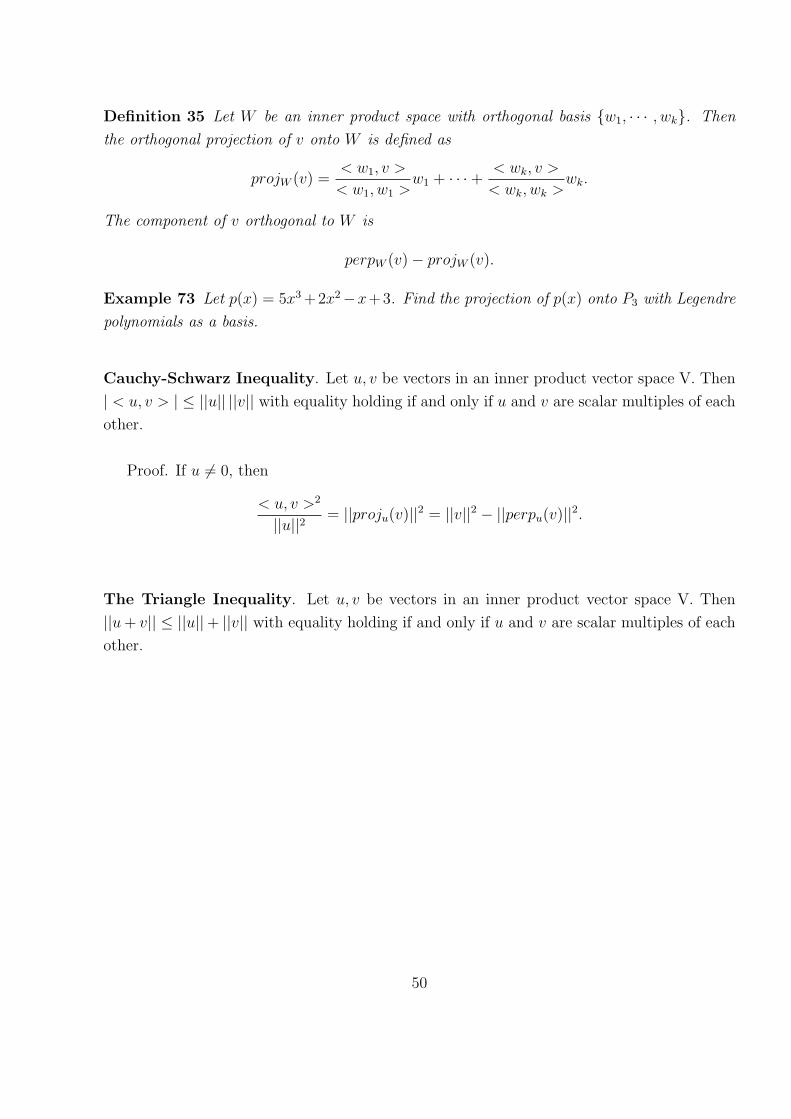
Definition 35 Let W be an inner product space with orthogonal basis {w1, · · · , wk}. Then

the orthogonal projection of v onto W is defined as

projW (v) =< w1, v >

< w1, w1 >w1 + · · ·+ < wk, v >

< wk, wk >wk.

The component of v orthogonal to W is

perpW (v)− projW (v).

Example 73 Let p(x) = 5x3+2x2−x+3. Find the projection of p(x) onto P3 with Legendre

polynomials as a basis.

Cauchy-Schwarz Inequality. Let u, v be vectors in an inner product vector space V. Then

| < u, v > | ≤ ||u|| ||v|| with equality holding if and only if u and v are scalar multiples of each

other.

Proof. If u ̸= 0, then

< u, v >2

||u||2= ||proju(v)||2 = ||v||2 − ||perpu(v)||2.

The Triangle Inequality. Let u, v be vectors in an inner product vector space V. Then

||u+ v|| ≤ ||u||+ ||v|| with equality holding if and only if u and v are scalar multiples of each

other.

50

7.2 Norms and Distance Functions

7.2.1 Norms

Definition 36 A norm on a vector space V is a mapping that associates with each vector v

a real number ||v|| such that, for all u, v and scalar c:

(a) ||v|| ≥ 0, and ||v|| = 0 if and only if v = 0.

(b) ||cv|| = |c|||v||.(c) ||u+ v|| ≤ ||u||+ ||v||.

A vector space along with a norm is called a normed linear space.

Example 74 Let u⃗ =

u1

u2

...

un

be a vector in Rn. i.e.

• The sum norm: ||u||s = |u1|+ |u2|+ · · ·+ |un|.

• The max norm (∞-norm, or uniform norm): ||u||∞ = max{|u1|, |u2|, · · · , |un|}.

• The sum norm: ||u||p = (|u1|p + |u2|p + · · ·+ |un|p)1/p . When p = 2, it is called Eu-

clidean norm.

Example 75 Let v ∈ Zn2 . Define ||v||H = w(v), the weight of v, which counts the number of

1’s in v. Then it is a norm, and called Hamming norm.

7.2.2 Distance Function

Definition 37 Form any norm, we define d(u, v) = ||u− v||.

Property 8 (a) d(u, v) ≥ 0, and d(u, v) = 0 if and only if v = u.

(b) d(u, v) = d(v, u).

(c) d(u,w) ≤ d(u, v) + d(v, w).

A function d satisfying the three properties is called metric. A vector space the possesses such

a function is called metric space.

51


1

2

3

, v⃗ =

4

4

4

. Calculate dE(u, v), ds(u, v), d∞(u, v).


1

1

0

, v⃗ =

0

1

1

∈ Z32. Calculate dH(u, v).

7.2.3 Matrix Norms

Definition 38 A matrix norm on Mnn is a mapping that associates with each matrix A a

real number ||A|| such that, for all A, B and scalar c:

(a) ||A|| ≥ 0, and ||A|| = 0 if and only if A = 0.

(b) ||cA|| = |c|||A||.(c) ||A+B|| ≤ ||A||+ ||B||.(d) ||AB|| ≤ ||A|| ||B||.

A matrix norm on Mnn is said to be compatible with a vector norm ||v|| on Rn if for all A

and x:

||Ax|| ≤ ||A|| ||x||.

Example 78 • The Frobenius norm:

||A||F =

√√√√ n∑i,j=1

a2ij.

1. Show that it is compatible with the Euclidean norm.

2. Show that it is a matrix norm.

• ||A||1 = max||x||=1 ||Ax|| defines another matrix norm. This norm is called operator

norm induced by the vector norm ||x||.

• ||A||1 = maxj=1,··· ,n {∑n

i=1 |aij|} = maxj=1,··· ,n {||aj||s} defines a matrix norm, where aj

is the j-th column of A.

• ||A||∞ = maxi=1,··· ,n

{∑nj=1 |aij|

}= maxi=1,··· ,n {||bi||s} defines a matrix norm, where bi

is the i-th column of A.

52

7.3 Least Squares Approximation

7.3.1 The Best Approximation Theorem

Definition 39 Let W be a subspace of a normed linear space V . Then for any v ∈ V , the

best approximation to v in W is the vector v̄ ∈ W such that

||v − v̄|| < ||v − w||

for any w ∈ W different from v̄.

The Best Approximation Theorem. Let W be a finite-dimensional subspace of an inner

product space V . Then for any v ∈ V , the best approximation to v in W is projW (v).

Proof. v − projW (v) is orthogonal to projW (v)− w.


1

1

1

1

, v⃗1 =

0

1

−2

1

, v⃗2 =

0

0

1

2

, v⃗3 =

0

−5

−2

1

. LetW = Span{v⃗1, v⃗2, v⃗3}.

Find the best approximation to y⃗ in W , i.e., projW y⃗.

Sol: Since

v⃗1 · v⃗2 = 0 + 0 + (−2) + 2 = 0

v⃗1 · v⃗3 = 0 + (−5) + 4 + 1 = 0

v⃗2 · v⃗3 = 0 + 0 + (−2) + 2 = 0.

Thus v⃗1⊥v⃗2, v⃗1⊥v⃗3, v⃗2⊥v⃗3, the set {v⃗1, v⃗2, v⃗3} is orthogonal basis of W.

projW y⃗ = ˆ⃗y =y⃗ · v⃗1v⃗1 · v⃗1

v⃗1 +y⃗ · v⃗2v⃗2 · v⃗2

v⃗2 +y⃗ · v⃗3v⃗3 · v⃗3

v⃗3 = 0

0

1

−2

1

+3

5

0

0

1

2

+−6

5

0

−5

−2

1

=

0

6

3

0

.

53

7.3.2 Least Squares Approximation

The line y = a + bx is called the line of best fit (or the leat squares approximating

line) for the points (x1, y1), · · · , (xn, yn), if it minimizes

(a+ bx1 − y1)2 + · · ·+ (a+ bxn − yn)

2 = ||Ax⃗− b⃗||,

where

A =

1 x1

1 x2

......

1 xn

, x⃗ =

[a

b

], b⃗ =

y1

y2...

yn

.

Definition 40 Let A be m × n matrix and b⃗ ∈ Rn, a least squares solution of Ax⃗ = b⃗ is a

vector y⃗ ∈ Rn such that

||⃗b− Ay⃗|| ≤ ||⃗b− Ax⃗||

for all x⃗ ∈ Rn.

The Least Squares Theorem. Let A be m×n matrix and b⃗ ∈ Rn, a least squares solution

of Ax⃗ = b⃗ always exists. Moreover:

a. X is a least squares solution of Ax⃗ = b⃗ if and only if X is a solution of the normal

equation

ATAx⃗ = AT b⃗.

b. A has linearly independent columns if and only if ATA is invertible. In this case, the

least squares solution of Ax⃗ = b⃗ is unique and given by

X = (ATA)−1AT b⃗.

Proof. a. Let AX = projcol(A)⃗b. Then (⃗b− AX)⊥col(A). Thus AT (⃗b− AX) = 0.

b. rank(A) = n if and only if ATA is invertible.

Example 80 Find the least squares approximating line for the data points (1,2), (2,2) and

(3,4).

54

Solution: Let the line be y = a+ bx. Then 1 1

1 2

1 3

[a

b

]=

2

2

4

.

The normal equation is: 1 1

1 2

1 3

T 1 1

1 2

1 3

[a

b

]=

1 1

1 2

1 3

T 2

2

4

,⇒

[3 6

6 4

][a

b

]=

[8

18

].

The solution is [a

b

]=

[3 6

6 4

]−1 [8

18

]=

[2/3

1

].

Remark. Similarly, we can find the parabola that gives the best least squares approximation

to data points.

7.3.3 Least Squares via the QR Factorization

Theorem 36 Let A be m × n matrix and b⃗ ∈ Rn. If A = QR is a QR factorization of A,

then the unique least squares solution of Ax⃗ = b⃗ is

X = R−1QT b⃗.

Proof. By the facts that QTQ = I and R is invertible.

Example 81 Use QR factorization to find a least squares solution of1 0 −3

0 2 −1

1 0 1

1 3 5

x⃗ =

1

1

1

1

.

Solution: By 5.3.2,1 0 −3

0 2 −1

1 0 1

1 3 5

=

1√3

− 1√10

− 3√23

0 2√10

− 3√23

1√3

− 1√10

1√23

1√3

2√10

2√23

√3

√3

√3

0√10

√10

0 0√23

.

55

7.3.4 Orthogonal Projection Revisited

Theorem 37 Let W be a subspace of Rm, and let A be m× n matrix whose columns form a

basis of W . If v ∈ Rm, then

projW (v) = A(ATA)−1ATv.

The linear transformation P that projects Rm onto W has A(ATA)−1AT as its standard matrix.

Proof. Let X be the unique leat squares solution of Ax = v. Then AX = projcol(A)(v) =

projW (v).

Example 82 Let W = {(x, y, z) ∈ R3|x − y + 2z = 0}. Find the orthogonal projection of

v = [3 − 1 2]T onto W and give the standard matrix of the linear transformation P that

projects R3 onto W .

Solution: Let A =

1 −1

1 1

0 1

, whose columns form a basis of W .

56

7.4 The Singular Value Decomposition

7.4.1 The Singular Values of a Matrix

Definition 41 Let A be m × n matrix. The singular values of A are the square roots of the

eigenvalues of ATA and are denoted by σ1, · · · , σn so that σ1 ≥ · · · ≥ simgan.

Example 83 Let A =

1 1

1 0

0 1

. Then sigma1 =√3, σ2 = 1.

7.4.2 The Singular Values Decomposition

The Singular Values Decomposition: Let A be m× n matrix. The singular values of A

satisfy σ1 ≥ · · · ≥ σr > 0, and σr+1 = · · ·σn = 0. Let

V = [v1 · · · vn],

where {v1, · · · , vn} is an orthonormal basis of Rn consisting of eigenvectors of ATA. Let

U = [u1 · · · um],

where {u1, · · · , um} is an orthonormal basis of Rm extended from the set

{u1, · · · , ur}, u1 =1

σ1

Av1, · · · , ur =1

σr

Avr.

Let

Σ =

[D O

O O

], D = diag{σ1, · · · , σr}.

Then

A = UΣV T ,

which is called a singular value decomposition (SVD) of A. The columns of U are called

left singular vectors of A, the columns of V are called right singular vectors of A.

Example 84 Let A =

1 1

1 0

0 1

. Find a singular value decomposition (SVD) of A.

57

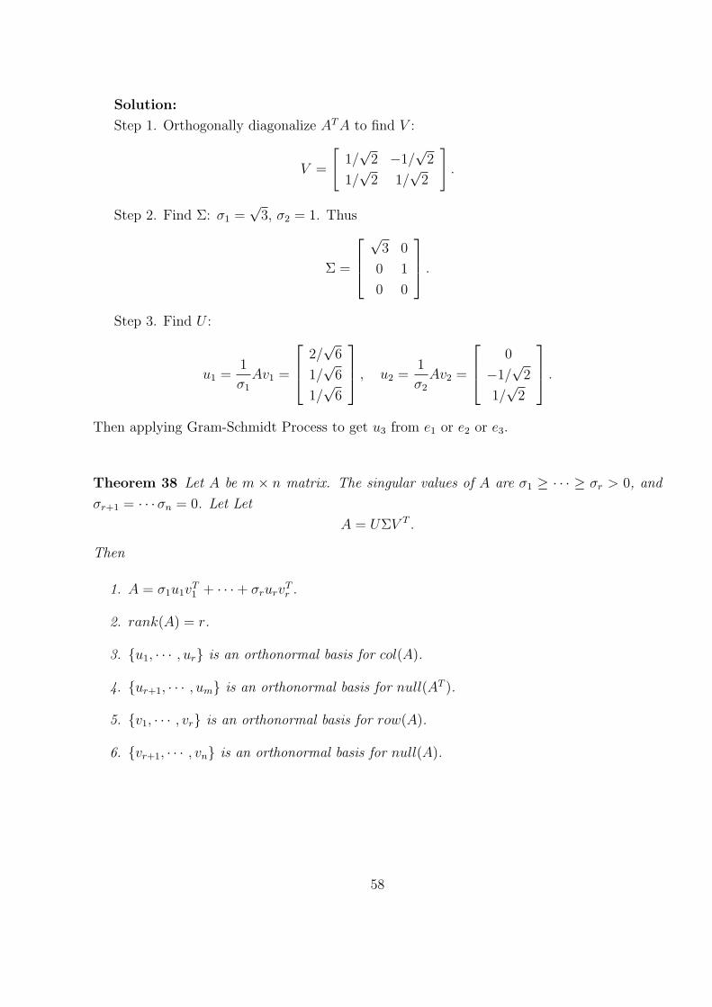
Solution:

Step 1. Orthogonally diagonalize ATA to find V :

V =

[1/√2 −1/

√2

1/√2 1/

√2

].

Step 2. Find Σ: σ1 =√3, σ2 = 1. Thus

Σ =

√3 0

0 1

0 0

.

Step 3. Find U :

u1 =1

σ1

Av1 =

2/√6

1/√6

1/√6

, u2 =1

σ2

Av2 =

0

−1/√2

1/√2

.

Then applying Gram-Schmidt Process to get u3 from e1 or e2 or e3.

Theorem 38 Let A be m × n matrix. The singular values of A are σ1 ≥ · · · ≥ σr > 0, and

σr+1 = · · · σn = 0. Let Let

A = UΣV T .

Then

1. A = σ1u1vT1 + · · ·+ σrurv

Tr .

2. rank(A) = r.

3. {u1, · · · , ur} is an orthonormal basis for col(A).

4. {ur+1, · · · , um} is an orthonormal basis for null(AT ).

5. {v1, · · · , vr} is an orthonormal basis for row(A).

6. {vr+1, · · · , vn} is an orthonormal basis for null(A).

58

Documents

Math2107 Notes