Forward.

These are step-by-verifiable-step notes designed to take students with a year of calculus based

physics who are about to enroll in ordinary differential equations all the way to doctoral foundations in

either mathematics and physics without mystery. Abstract algebra, topology (local and global) folds into

a useful, intuitive toolset for ordinary differential equations and partial differential equations, be they

linear or nonlinear. The algebraist, the topologist, the theoretical physicist, the applied mathematician

and experimental physicist are artificial distinctions at the core. There is unity.

Mathematician, you will see step-by-verifiable-step algebra, topology (local and global) in a

unified framework to treat differential equations, ordinary, partial, linear and nonlinear. You will then

see why the physicists created a great font of differential equations, the calculus of variations. You will

see why the physicists care about both discrete and continuous (topological) Lie groups and understand

what quantum mechanics is as a mathematical system from its various historical classical physical roots:

Lagrangian mechanics, Hamiltonian mechanics, Poisson brackets. You will have the tools to understand

the Standard Model of physics and some of our main paths forward to grand unified theories and

theories of everything. With these notes you should never again be able to practice abstraction for the

sake of abstraction. Physicist, you will not be held hostage to verbiage and symbology. You will see that

mathematics has deep, unavoidable limitations that underlie physics, itself suffering unavoidable

limitations. You will see unity, e.g., summing angular momentum in terms of tensor products and

directions sums, ladder operators, Young’s tableaux, root and weigh diagrams as different codifications

of the same thing. Neither of you have to take your required courses as exercises in botany and voodoo

as exemplified by ordinary differential equations. You will have context and operational skills. As

lagniappes you will have the calculus of variations, the fractional calculus, stochastic calculus and

stochastic differential equations.

i

Contents

Part I. (p. 1) Assuming only a mathematical background up to a sophomore level course in

ordinary differential equations, Part I treats the application of symmetry methods for differential

equations, be they linear, nonlinear, ordinary or partial. The upshot is the development of a naturally

arising, systematic abstract algebraic toolset for solving differential equations that simultaneously binds

abstract algebra to differential equations, giving them mutual context and unity. In terms of a semester

of study, this material would best follow a semester of ordinary differential equations. The algorithmics,

which will be developed step by step with plenty of good examples proceed along as follows: (1) learn to

use the linearized symmetry condition to determine the Lie point symmetries, (2) calculate the

commutators of the basis generators and hence the sequence of derived subalgebras, (3) find a

sufficiently large solvable subalgebra, choose a canonical basis, calculate the fundamental differential

invariants, and (4) rewrite the differential equation in terms of any differential invariants; then use each

generator in turn to carry out one integration. This sounds like a mouthful, but you will see that it is not.

The material is drawn from my notes derived from “Symmetry Methods for Differential Equations: A

Beginner’s Guide,” Peter E. Hydon, Cambridge University Press, 2000.

Part II. (p. 125) Part II which assumes no additional background, should be learned in parallel

with Part I. Part II builds up the calculus of variations by paralleling the buildup of undergraduate

elementary calculus. Present day physics including classical mechanics, electrodynamics, quantum

physics, quantum field theories, general relativity, string theories, and loop quantum gravity, for

example, are all expressed in terms of some variational principle extremizing some action. This

extremization process leads to, through the calculus of variations, sets of differential equations. These

differential equations have associated symmetries (Part I) that underlie our present understanding of

fundamental physics, the Standard Model. The same goes for many of the theoretical symmetries

ii

stretching beyond the Standard Model such as grand unified theories (GUTs) with or without

supersymmetry (SUSY), and theories of everything (TOEs) like string theories. We will buttress the use

of this variational toolset with history. Part II will thus provide us a deep, practical, intuitive source of

differential equations, while Part I places the investigation of these differential equations in a general,

practical, intuitive, algebraic framework readily accessible to the college sophomore. The variational

material is drawn from “Calculus of Variations (Dover Books on Mathematics),” Lev D. Elsgolc, Dover

Publications, 2007.

Beyond the sophomore level material contained in Parts I and II, a student pursuing deeper

studies in either physics or mathematics will have already been well served by these notes, forever

understanding that most abstract mathematics is likely clothed within a rich, intuitively unified, and

useful context, and that any voodoo mathematical prescriptions in physics can be deconstructed from a

relatively small collection of fundamental mathematical tools and physical principles. It would be

desirable, but not necessary for studying Parts I and II, to have had some junior level exposure to

classical mechanics motivating the calculus of variations. In lieu of this, I strongly recommend parallel

readings from “Variational Principles In Dynamics and Quantum Theory (Dover Books on Physics)”,

Wolfgang Yourgrau and Stanley Mandelstam, Dover Publications, 1979 to tie the calculus of variations to

mechanics, quantum mechanics and beyond through the historical development of this field from

Fermat to Feynman.

Part III. (p. 136) Part III culminates the unifying goal of Parts I and II at the junior level, intuitively

unifying algebra and topology together into algebraic topology with applications to differential

equations and physics. Whereas in Part I students learn to study the sub-algebraic structure of the

commutators of a differential equation to learn if a given differential equation may be more readily

solved in new coordinates and/or reduced in order, Part III begins to develop the topological linkage of

iii

commutators to quantum field theories and general relativity by intuitively developing the concepts

underlying parallel transport and the covariant derivative. This picture is developed step-by-step free of

hand waving. It is recommended that the material in Part III be studied in parallel with a traditional

junior level course in partial differential equations. If you are doing Part III solo, the parallel material for

partial differential equations can be found in, “Applied Partial Differential Equations with Fourier Series

and Boundary Value Problems,” 4th ed., Richard Haberman, Prentice Hall, 2003—a great text in any

edition. Having a junior level background in classical mechanics up to the Lagrangian and Hamiltonian

approaches would greatly add to the appreciation of Parts I, II, and III. In lieu of this background is a

reading of the previously cited Dover history book by Wolfgang Yourgrau and Stanley Mandelstam. The

material covering algebraic topology and differential equations is drawn from the first four chapters of

“Lie Groups, Lie Algebras, and Some of Their Applications (Dover Books on Mathematics)”, Robert

Gilmore, Dover Publications, 2006. Part III cleans up and fills in Gilmore’s Dover book. The nitty gritty

connections to quantum field theories and general relativity can be further elaborated from reading

chapter three of “Quantum Field Theory,” 2nd ed., Lewis H. Ryder, Cambridge University Press, 1996, and

from “A Short Course in General Relativity,” 3rd ed., James A. Foster and J. David Nightingale, Springer,

2005. The latter book provides a step by step construction of general relativity including the concept of

parallel transport and the covariant derivative from a geometric point of view.

Part IV. (p. 207) In Part IV machinery is built up to study the group theoretic structures

associated, not with differential equations this time, but with polynomials to prove the insolvability of

the quintic, now providing the student with two examples of the utility of abstract algebra and linear

algebra to problems in mathematics. As we develop this machinery, we will study the properties of the

irreducible representations of discrete groups with applications to crystallography, molecular vibrations,

and quantum physics. The toolset is then extended to continuous groups with applications to quantum

physics and particle physics. It will be shown how to use ladder algebras to solve quantum mechanical

iv

differential equations algebraically. No step will be left out to mystify students. The material dealing

with the insolvability of the quintic and discrete groups is pulled from two sources, Chapter 1 of “Lie

Groups, Physics, and Geometry: An Introduction for Physicists, Engineers and Chemists,” Robert

Gilmore, Cambridge University Press, 2008, and from the first four chapters of the first edition of

“Groups, Representations and Physics,” 2nd ed., H. F. Jones, Institute of Physics Publishing, 1998. The

latter, 2008 book by Robert Gilmore is too fast paced, and too filled with hand waving to serve other

than as a guide for what is important to learn after learning the material presented in this work. The

material dealing with continuous groups is derived from many sources which I put together into a set of

notes to better understand “An Exceptionally Simple Theory of Everything,” A. Garrett Lisi,

arXiv:0711.0770v1, 6 November 2007.

A note on freebies. It is assumed that the student will take a course in complex analysis at the

level of any late edition of “Complex Variables and Applications,” James W. Brown and Ruel V. Churchill,

McGraw-Hill Science/Engineering/Math, 8th ed., 2008. Strongly recommended are one or two good

courses in linear algebra. A physics student, typically at the graduate level, is usually required to take a

semester of mathematical physics covering a review of undergraduate mathematics and a treatment of

special functions and their associated, physics-based differential equations. Once again the student is

back to studying botany, and once again symmetry groups unify the botany. A free book treating this

can be downloaded from http://www.ima.umn.edu/~miller/lietheoryspecialfunctions.html (“Lie Theory

and Special Functions,” by Willard Miller, Academic Press, New York, 1968 (out of print)).

A note on step-by-step books. “Introduction to Electrodynamics,” 3rd ed., David J. Griffiths,

Benjamin Cummings, 1999, or equivalent level of junior level electrodynamics, “Quantum

Electrodynamics,” 3rd ed., Greiner and Reinhardt, Springer 2002, and “Quantum Field Theory,” 2nd ed.,

Lewis H. Ryder, Cambridge University Press, 1996 are each excellent, clearly written and self-contained.

v

Griffiths should be read from end to end. Greiner and Reinhardt should be read up to at least chapter

four, if not up to chapter five to gain hands-on experience with calculating cross sections and decay

rates the old fashioned way that led Richard Feynman to develop the Feynman diagram approach. The

introductory chapter of Ryder may be skipped. Chapters two and three are where the physics and the

mathematics lay that are relevant to much of the material presented in this work. The introductory

chapter on path integrals is also pertinent.

Part V. (p. 294) Part V treats a miscellany of topics. Principal among these topics is material

drawn from “The Fractional Calculus, Theory and Applications of Differentiation and Integration to

Arbitrary Order (Dover Books on Mathematics)” by Keith B. Oldham and Jerome Spanier, Dover

Publications, 2006. You will not only come to appreciate the gamma function better, you will be able to

ask if the √ th derivative has any meaning. Who said we can only take 1st, 2nd,…,nth order derivatives, or

integrate once, twice,…,or n times? Calculus is more general, more unified, more intuitive, and more

physical than calculus with only integer order differentiation or integration. The conversation will then

turn to stochastic processes (p. 301). In my studies, I found measure theoretic analysis to be another

source of meaningless, isolated, dry crap until I got into financial physics and needed to work with

stochastic differential equations. Finance and statistical physics, to a lesser extent as currently taught in

graduate physics courses, give context to measure theory. Material to show this is taken from “Options,

Futures, and Other Derivatives,” 5th (or higher) edition, John C. Hull, Prentice Hall, 2002, as well as from

personal notes.

Here is a final word to the physicists. Parts I and II of this work go to support graduate level

classical mechanics and its extensions to quantum physics and quantum field theory. You should

buttress your understanding of classical mechanics beyond the standard graduate course covering the

material in, say, “Classical Mechanics,” 3rd ed., Herbert Goldstein, Addison Wesley, 2001. Goldstein

vi

certainly provides a good treatment of classical mechanics, giving the reader the background underlying

the development of quantum physics, but he does not cover continuum mechanics. Continuum

mechanics is not just for the engineer. The development of tensors and dyadic tensors is far greater in

continuum mechanics than in typical, introductory general relativity. It is your loss not to acquire this

more general toolset. I recommend, “Continuum Mechanics (Dover Books on Physics),” A. J. M.

Spencer, Dover Publications, 2004. To complete one’s understanding of mechanics, one should also

study “Exploring Complexity,” G. Nicolis and I. Prigogine, W H Freeman, 1989. Moving from complexity

to statistical physics, my favorite statistical physics book is “A Modern Course in Statistical Physics,”

Linda E. Reichl, Wiley-VCH, 2009 (or its older edition). For experience solving practical problems, study

“Statistical Mechanics (North-Holland Personal Library)”, R. Kubo, H. Ichimura, T. Usui, and N.

Hashitsume, North Holland, 1990. Underlying statistical physics is thermodynamics. I recommend

“thermodynamics (Dover Books on Physics)” by Enrico Fermi, Dover Publications, 1956. “An

Introduction to equations of state: theory and applications” by S. Eliezer, A. G. Ghatak and H. Hora

(1986) gives a pretty good treatment of where our knowledge in thermodynamics and statistical physics

abuts our ignorance, as well as shows how quickly mathematical models and methods become complex,

difficult and approximate. This compact book has applications far outside of weapons work to work in

astrophysics and cosmology. Rounding out some of the deeper meaning behind statistical physics is

information theory, I recommend reading “The Mathematical Theory of Communication” by Claude E.

Shannon and Warren Weaver, University of Illinois Press, 1998, and “An Introduction to Information

Theory, Symbols, Signals and Noise” by John R. Pierce (also from Bell Labs), Dover Publications Inc.,

1980. The material covered in Part V on measure theory and stochastic differential equations fits well

with the study of statistical physics.

Parts I and II also go to the study of electrodynamics, undergraduate and graduate. At the

graduate level (“Classical Electrodynamics,” 3rd ed., John D. Jackson, Wiley, 1998) one is inundated with

vii

differential equations and their associated special functions. The online text by Willard Miller tying

special functions to Lie symmetries is very useful at this point. I also recommend an old, recently

reprinted book, “A Course of Modern Analysis,” E. T. Whittaker, Book Jungle, 2009. The historical

citations, spanning centuries, are exhaustive.

Parts I through V of this work underlie studies in general relativity, quantum mechanics,

quantum electrodynamics and other quantum field theories. With this background you will have better

luck reading books like, “A First Course in Loop Quantum Gravity,” R. Gambini and J. Pullin, Oxford

University Press, 2011, and “A First Course in String Theory,” Barton Zweibach, 2nd ed., Cambridge

University Press, 2009. Again, only together do mathematics and physics provide us with a general,

intuitive grammar and powerful, readily accessible tools to better understand and explore nature and

mathematics, and even to help us dream and leap beyond current physics and mathematics. Before you

get deep into particle physics, I recommend starting with “Introduction to Elementary Particles,” 2nd ed.,

David Griffiths, Wiley-VCH, 2008.

A. Alaniz

Apologies for typos in this first edition, December 2012. Teaching should be more than about how, but

also about why and what for. Read this stuff in parallel, in series, and check out other sources. Above

all, practice problems. The file “Syllabus” is a words based syllabus for the mathematician and physicist,

and a recounting of the origin of some of the main limitations of mathematics and physics.

1

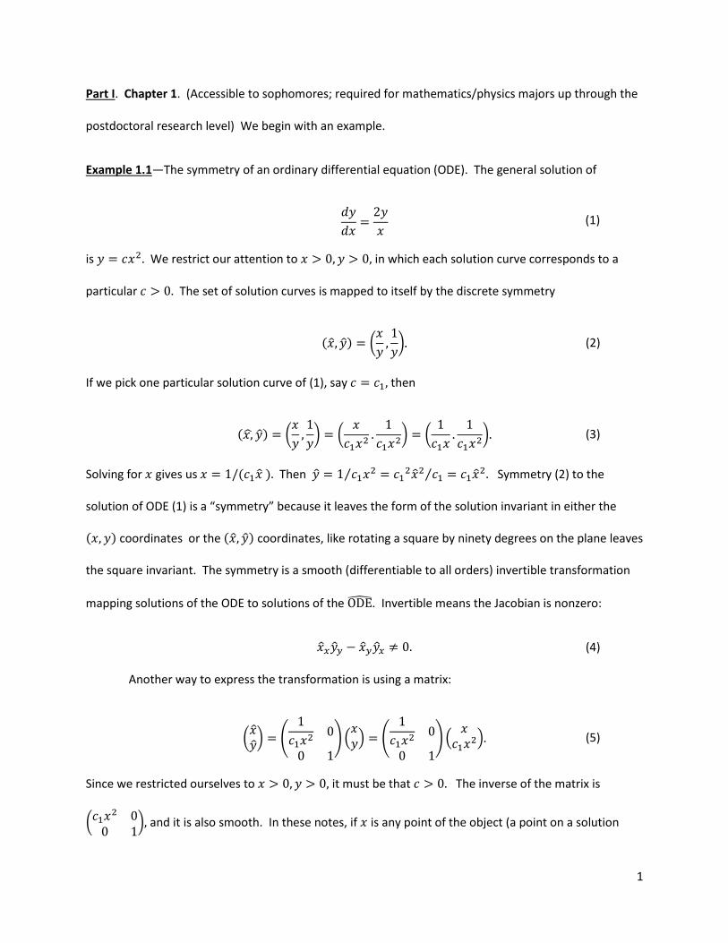
Part I. Chapter 1. (Accessible to sophomores; required for mathematics/physics majors up through the

postdoctoral research level) We begin with an example.

Example 1.1—The symmetry of an ordinary differential equation (ODE). The general solution of

(1)

is We restrict our attention to in which each solution curve corresponds to a

particular The set of solution curves is mapped to itself by the discrete symmetry

( ) (

) (2)

If we pick one particular solution curve of (1), say then

( ) (

) (

) (

) (3)

Solving for gives us ( ) Then ⁄

⁄ Symmetry (2) to the

solution of ODE (1) is a “symmetry” because it leaves the form of the solution invariant in either the

( ) coordinates or the ( ) coordinates, like rotating a square by ninety degrees on the plane leaves

the square invariant. The symmetry is a smooth (differentiable to all orders) invertible transformation

mapping solutions of the ODE to solutions of the . Invertible means the Jacobian is nonzero:

(4)

Another way to express the transformation is using a matrix:

( ) (

) ( ) (

) (

) (5)

Since we restricted ourselves to it must be that The inverse of the matrix is

(

) and it is also smooth. In these notes, if is any point of the object (a point on a solution

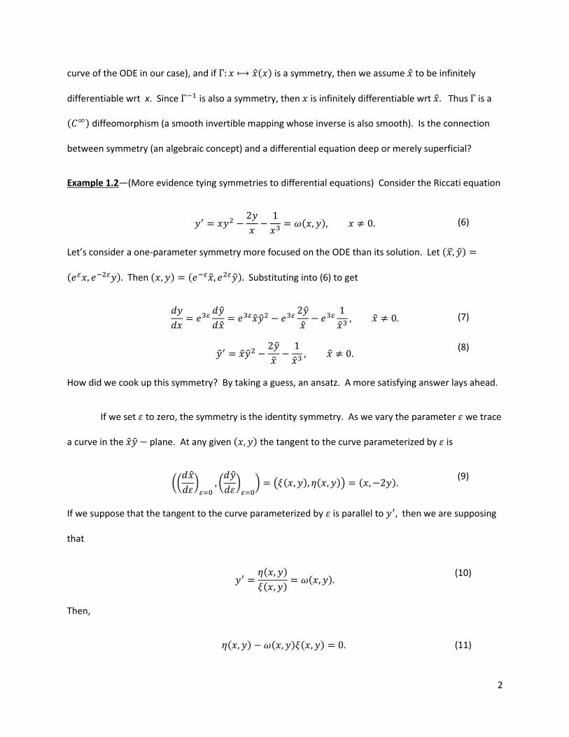
2

curve of the ODE in our case), and if ( ) is a symmetry, then we assume to be infinitely

differentiable wrt x. Since is also a symmetry, then is infinitely differentiable wrt Thus is a

( ) diffeomorphism (a smooth invertible mapping whose inverse is also smooth). Is the connection

between symmetry (an algebraic concept) and a differential equation deep or merely superficial?

Example 1.2—(More evidence tying symmetries to differential equations) Consider the Riccati equation

( ) (6)

Let’s consider a one-parameter symmetry more focused on the ODE than its solution. Let ( )

( ) Then ( ) ( ) Substituting into (6) to get

(7)

(8)

How did we cook up this symmetry? By taking a guess, an ansatz. A more satisfying answer lays ahead.

If we set to zero, the symmetry is the identity symmetry. As we vary the parameter we trace

a curve in the plane. At any given ( ) the tangent to the curve parameterized by is

((

)

(

)

) ( ( ) ( )) ( ) (9)

If we suppose that the tangent to the curve parameterized by is parallel to then we are supposing

that

( )

( ) ( )

(10)

Then,

( ) ( ) ( ) (11)

3

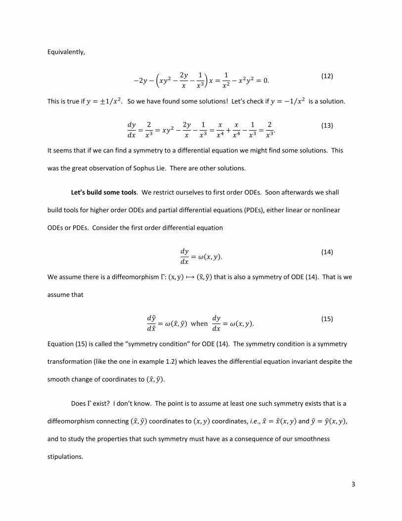
Equivalently,

(

)

(12)

This is true if ⁄ So we have found some solutions! Let’s check if ⁄ is a solution.

(13)

It seems that if we can find a symmetry to a differential equation we might find some solutions. This

was the great observation of Sophus Lie. There are other solutions.

Let’s build some tools. We restrict ourselves to first order ODEs. Soon afterwards we shall

build tools for higher order ODEs and partial differential equations (PDEs), either linear or nonlinear

ODEs or PDEs. Consider the first order differential equation

( )

(14)

We assume there is a diffeomorphism ( ) ( ) that is also a symmetry of ODE (14). That is we

assume that

( )

( )

(15)

Equation (15) is called the “symmetry condition” for ODE (14). The symmetry condition is a symmetry

transformation (like the one in example 1.2) which leaves the differential equation invariant despite the

smooth change of coordinates to ( ).

Does exist? I don’t know. The point is to assume at least one such symmetry exists that is a

diffeomorphism connecting ( ) coordinates to ( ) coordinates, i.e., ( ) and ( )

and to study the properties that such symmetry must have as a consequence of our smoothness

stipulations.

4

Relating ⁄ to the original coordinates ( ) is the total derivative

. In this notation, subscript Latin letters imply differentiation wrt that Latin letter, e.g.,

⁄ . Keeping only terms up to first order

(16)

The symmetry condition (15) for ODE (14) yields

( )

( )

(17)

Since ( ) in the original coordinates, and we may write

( )

( ) ( )

(18)

Equation (18) together with the requirement that is a diffeomorphism is equivalent to the symmetry

condition (15). Equations (17) or (18) tie (or “ligate”) the original coordinates ( ) to the new

coordinates ( ( ) ( )) This result is important because it may lead us to some if not all of the

symmetries of an ODE. Was the symmetry to the Riccati equation pulled from the ass of some genius,

or was there a method to the madness? (Notice the Riccati equation is nonlinear.)

Example 1.3—To better understand the hunt for symmetries, consider the simple ODE

(19)

Symmetry condition (17) implies that each symmetry of (19) satisfies the PDE

Since in the original ( )coordinates, equation (18) equivalently implies that

5

(20)

Rather than trying to find the general solution to this PDE, let us instead use (20) to inspire some simple

guesses at some possible symmetries to ODE (19). Say we try ( ) ( ( ) ) That is is only a

function of and not of i.e., Then and (20) reduces to

(21)

or,

(22)

For any symmetries which are diffeomorphisms, the Jacobian is nonzero. That is,

(23)

The simplest case of is . So the simplest one-parameter symmetry to ODE (19) is

( ) ( ) (24)

Let’s check by substituting this into the LHS and RHS of (17).

{

}

{ } (25)

The diffeomorphism ( ) ( ) is therefore a symmetry of ODE (19). We now have some hope

that producing the symmetry to the Riccati equation may have more to it than a genius’ guess. There

are more powerful, more systematic methods to come.

WARNING!!! Eleven double spaced pages with figures and examples follow before we treat the

Riccati equation with a more complete set of tools (feel free to peek at example 1.8). Most of the

material is fairly transparent on first reading, but some of it will require looking ahead to the fuller

Riccati example (example 1.8), going back and forth through these notes.

6

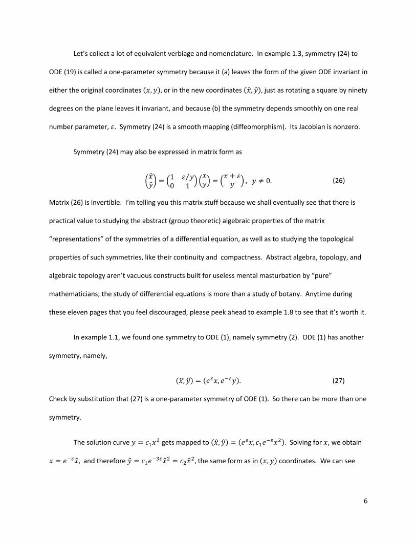
Let’s collect a lot of equivalent verbiage and nomenclature. In example 1.3, symmetry (24) to

ODE (19) is called a one-parameter symmetry because it (a) leaves the form of the given ODE invariant in

either the original coordinates ( ) or in the new coordinates ( ) just as rotating a square by ninety

degrees on the plane leaves it invariant, and because (b) the symmetry depends smoothly on one real

number parameter, . Symmetry (24) is a smooth mapping (diffeomorphism). Its Jacobian is nonzero.

Symmetry (24) may also be expressed in matrix form as

( ) (

⁄

)( ) (

) (26)

Matrix (26) is invertible. I’m telling you this matrix stuff because we shall eventually see that there is

practical value to studying the abstract (group theoretic) algebraic properties of the matrix

“representations” of the symmetries of a differential equation, as well as to studying the topological

properties of such symmetries, like their continuity and compactness. Abstract algebra, topology, and

algebraic topology aren’t vacuous constructs built for useless mental masturbation by “pure”

mathematicians; the study of differential equations is more than a study of botany. Anytime during

these eleven pages that you feel discouraged, please peek ahead to example 1.8 to see that it’s worth it.

In example 1.1, we found one symmetry to ODE (1), namely symmetry (2). ODE (1) has another

symmetry, namely,

( ) ( ) (27)

Check by substitution that (27) is a one-parameter symmetry of ODE (1). So there can be more than one

symmetry.

The solution curve gets mapped to ( ) (

). Solving for , we obtain

and therefore

the same form as in ( ) coordinates. We can see

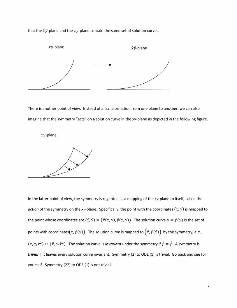
7

that the -plane and the -plane contain the same set of solution curves.

There is another point of view. Instead of a transformation from one plane to another, we can also

imagine that the symmetry “acts” on a solution curve in the xy-plane as depicted in the following figure.

In the latter point of view, the symmetry is regarded as a mapping of the xy-plane to itself, called the

action of the symmetry on the xy-plane. Specifically, the point with the coordinates ( ) is mapped to

the point whose coordinates are ( ) ( ( ) ( )) The solution curve ( ) is the set of

points with coordinates( ( )). The solution curve is mapped to ( ( )) by the symmetry, e.g.,

( ) (

). The solution curve is invariant under the symmetry if A symmetry is

trivial if it leaves every solution curve invariant. Symmetry (2) to ODE (1) is trivial. Go back and see for

yourself. Symmetry (27) to ODE (1) is not trivial.

𝑥𝑦-plane 𝑥��-plane

𝑥𝑦-plane

8

A one-parameter symmetry depends on only one-parameter, e.g., . A one-parameter

symmetry may look like ( ) ( ) or like ( ) ( ) A two-parameter

symmetry may look like ( ). We restrict ourselves to one-parameter symmetries until

further notice.

Group theory basics. It is time to note that our one-parameter symmetries are groups in the

sense of modern algebra. Why? To masturbate with nomenclature as you do in an abstract algebra

class? No. Because, as you will soon see, studying the group structure of a symmetry of a differential

equation will have direct relevance to reducing its order to lower order, and will have direct relevance to

finding some, possibly all of the solutions to the given differential equation—ordinary, partial, linear, or

nonlinear. So what is a group?

A group is a set G together with a binary operation * such that

(I) There is an element of , called the identity ( ), such that if the (Identity)

From ODE (1) with symmetry ( ) ( ) we see that ( ) ( ) ( ) when

The identity element doesn’t do jack. It has no action.

(II) For every ( ) there exists ( ) a such that ( ) (Inverse)

The inverse to the symmetry for ODE (1) ( ) ( ) is ( ). Actually, these two

symmetries are their own inverses. The first symmetry “moves” ( ) to ( ) Applying the

inverse moves you back to ( ) ( ) In the symmetry we are using, you could reverse

the order and get the same result, but this is not always the case. Not everything is commutative

(Abelian). Cross products of three dimensional Cartesian vectors, for example, are not commutative

(non Abelian). (Titillation: Noncommutativity underlies quantum physics. You will see

this before you finish this set of notes.)

9

(III) If then (Closure)

If denotes ( ) and denotes ( ) then denotes ( ) which

is a member of Note that since the group is a continuous group.

(IV) If then ( ) ( ) (Associativity)

Check this yourself as we checked property (III). Lastly note that since the parameters are continuous,

the groups are continuous groups. Lots of diverse mathematical structures are groups.

Example 1.4—The set of even integers together with addition being * is a discrete group. Check the

definition.

Example 1.5—The set of polynomials together with the rules of polynomial addition being * is a group.

Example 1.6—The set of matrices that are invertible (have inverses) form a group with matrix

multiplication being *. The identity is the matrix with ones in the diagonal and zeros otherwise.

That is, (

) (Hint: In linear algebra we learn about matrices that are commutative, and matrices

that are not commutative—this stuff underlies quantum physics.)

The symmetry (27) to ODE (1) is, moreover, an infinite one-parameter group because the

parameter is a real number on the real number line. In example 1.3, we met an infinite set of

continuously connected symmetries, namely, ( ) ( ). This symmetry smoothly maps the

plane to the plane Later on, with ODEs of higher than first order, we shall deal with symmetries

from to , from to , and so on from to . These symmetries are called “Lie” groups

after Sophus Lie, the dude who brought them to the fore to deal with differential equations. We deal

with two more chunks of additional structure before getting back to practical, step-by-step applications

to linear and nonlinear differential equations.

10

Theorem I. Let us suppose that the symmetries of

( ) include the Lie group of

translations ( ) ( ) for all in some neighborhood of zero. Then,

( ) ( )

therefore when so does

( ) ( )

and therefore

( ) ( )

( )

Thus the function only depends on Thus

( ) and ∫ ( ) The particular

solution corresponding to is mapped by the translation symmetry to ∫ ( )

∫ ( ) which is the solution corresponding to Note—A differential equation is

considered solved if it has been reduced to quadrature—all that remains, that is, is to evaluate an

integral. Also note that this theorem will be deeply tied to the use of canonical coordinates up ahead.

Action. It is useful to study the action of one-parameter symmetries on points of the plane. The

orbit of a one-parameter Lie group through ( ) is a set of points to which ( ) can be mapped by a

specific choice of

( ) ( ( ) ( )) (28)

with initial condition

( ( ) ( )) ( ) (29)

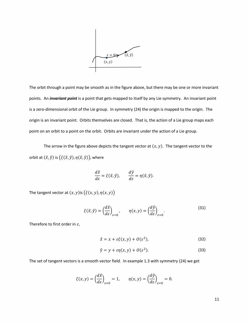
11

The orbit through a point may be smooth as in the figure above, but there may be one or more invariant

points. An invariant point is a point that gets mapped to itself by any Lie symmetry. An invariant point

is a zero-dimensional orbit of the Lie group. In symmetry (24) the origin is mapped to the origin. The

origin is an invariant point. Orbits themselves are closed. That is, the action of a Lie group maps each

point on an orbit to a point on the orbit. Orbits are invariant under the action of a Lie group.

The arrow in the figure above depicts the tangent vector at ( ). The tangent vector to the

orbit at ( ) is ( ( ) ( )) where

( )

( )

The tangent vector at ( )is ( ( ) ( ))

( ) (

)

( ) (

)

(31)

Therefore to first order in

( ) ( ) (32)

( ) ( ) (33)

The set of tangent vectors is a smooth vector field. In example 1.3 with symmetry (24) we get

( ) (

)

( ) (

)

(𝑥 𝑦)

(�� ��) 휀

12

Plugging the above into equations (32) and (33) we get and which is symmetry (24). I

was just checking that all of this stuff is consistent. Note that an invariant point is mapped to itself by

every Lie symmetry. Thus for an invariant point, we have ( ) ( ) from (32) and (33). It’s

alright if this stuff doesn’t yet mean much. It will soon allow us to find, if possible, a change of

coordinates that may allow a given differential equation to be reduced to a simpler form. The first

application will be to finding more solutions to the Riccati equation in “canonical” coordinates.

Characteristic equation. This next block of structure follows directly from example 1.2. See the

paragraph containing equations (9) through (12) in example 1.2. Any curve C is an invariant curve

( ) if and only if (iff) the tangent to C at each ( ) is parallel to the tangent vector

( ( ) ( )) This is expressed by the characteristic equation

( ) ( ) ( ) (34)

C is parallel to ( ) iff ( ) on C, or

( )

( )

(35)

This implies that

( )

(36)

can have its invariant solution characterized by

( ( )) ( ) ( ) (37)

Equation (37) is the reduced characteristic.

The new shorthand applied to the Riccati equation in example 1.2 updates that example to the

following. We were given

( ) The ansatz was ( )

( ) The tangent vector is ( ) ( ) The reduced characteristic is ( )

13

( ) ( ) (

)

( ) iff ( )

, the

“invariant solutions”. Most symmetry methods use the tangent vectors rather than the symmetries

themselves to seek out “better” coordinates to find solutions to differential equations.

Canonical coordinates. We use canonical coordinates when the ODE has Lie symmetries

equivalent to a translation. Symmetry (24) gives us an example of a symmetry to an ODE which is a

translation ( ) ( ) The ODE is greatly simplified under a change of coordinates to canonical

coordinates, e.g., the Riccati equation

( ) turns to

Given ( ) ( ) with tangent vector ( ( ) ( )) ( ) we seek coordinates

( ) ( ( ) ( )) such that ( ) ( ) Then the tangent vector is ((

)

(

)

) Using

( )

( ) and the chain rule

(38)

(39)

we get

( ) ( ) (40)

( ) ( ) (41)

By smoothness the Jacobian is not zero. That is,

(42)

Therefore a curve of constant and a curve of constant cross transversely. Any pair of functions

( ) ( ) satisfying (40) through (42) is called a pair of canonical coordinates. The curve of

constant corresponds (locally) with the orbit through the point ( ). The orbit is invariant under the

14

Lie group, so is the invariant canonical coordinate. Note that canonical coordinates cannot be defined

at an invariant point because the determining equation for , namely ( ) ( ) has no

solution if but it is always possible to normalize the tangent vectors (at least locally). Also

note that canonical coordinates defined by (40) and (41) are not unique. If ( ) satisfy (40) and (41) so

do ( ) ( ( ) ( )) (Thus, without proof there is a degeneracy condition which states

( ) but there is still plenty of freedom left.)

Canonical coordinates can be obtained from (40) and (41) through the method of

characteristics. In the theory of ODEs, the characteristic equation is

( )

( )

(43)

This is a system of ODEs. Here follows a definition. A first integral of a given first-order ODE

( )

(44)

is a nonconstant function ( ) whose value is constant on any solution ( ) of the ODE.

Therefore on any solution curve ( )

(45)

( )

(46)

The general solution is ( ) Suppose that ( ) in equation (40). Then let’s rearrange

equation (40) as

( )

( ) ( )

(47)

Comparing (46) with (40), we see that the is a first integral of

15

( )

( )

(48)

So ( ) is found by solving (48). It is an invariant canonical coordinate. Sometimes we can

determine a solution ( ) by inspection, else we can use ( ) to write as a function of and

The coordinate ( ) is obtained from (43) by quadrature:

( ) (∫

( ( ))) ( )

(49)

where is being treated as a constant.

If ( ) and ( ) then the canonical coordinates are

( ) (∫

( ))

(50)

Example 1.7—Every ODE of the form ( ⁄ ) admits the one-parameter Lie group of scalings

( ) ( ) Consider

as a very simple example (of course we know is the

solution). If the canonical coordinate is Then ( ) ∫

| |

Thus ( ) ( | |) At we need a “new coordinate patch”:

| | So

what? Finding canonical coordinates reduces ugly ODEs into simpler ODEs. We’re steps away from this.

Recall that Lie symmetries of an ODE are nontrivial iff

( ) ( ) ( ) (51)

If ODE (14),

( ) has nontrivial Lie symmetries equivalent to a translation, it can be reduced to

quadrature by rewriting it in terms of canonical coordinates as follows. Let

( )

( )

(52)

16

The right hand side of (52) can be written as a function of and using the symmetry. For a general

change of variables ( ) ( ) the transformed ODE (52) would be of the form

( )

(53)

for some function However, since we assume ( ) are canonical coordinates, the ODE is invariant

under the group of translations in the direction:

( ) ( ) (54)

Thus from theorem I we know that

( ) (55)

and therefore

( )

(56)

The ODE has been reduced to quadrature, and the general solution to ODE (56) is

( ) ∫ ( )

(57)

Therefore the general solution to ODE (14) is

( ) ∫ ( )

( )

(58)

This is great, but of course we must first determine the canonical coordinates by solving

( )

( )

(48)

Example 1.8—Let’s finally compute the Riccati equation with both barrels using our updated toolset.

( ) (6)

17

As we know, a symmetry of (6) is ( ) ( ) The corresponding tangent vector is

( ) ( ) The reduced characteristic ( ( )) ( ) ( ) ( ) is

( ( )) (

)

(59)

( ( )) iff

. We stopped here before. Now we use our symmetry’s tangent vector

to give us canonical coordinates to simplify the Riccati equation. Equation (48) becomes

( )

( )

(60)

The solution is

Thus and ( ) (∫

( ( ))) ( )

(∫

) ( )

| | Thus our canonical coordinates are

( ) ( | |) (61)

Of course and So

Plug into equation (52):

( )

( )

( )

(62)

The Riccati equation has been reduced to quadrature in the canonical coordinates. That is

( ) (∫

)

(63)

Converting back to the original coordinates we get

| |

|

| | | |√

| |√

|

(64)

(65)

18

(66)

( ) (67)

( )

(68)

We have solved the Riccati equation. We can get back the two solutions that were derived using the

reduced characteristic equation by taking limits:

and

Note for sticklers,

the “Riccati” equation is actually any ODE that is quadratic in the unknown function. It is nonlinear. We

can solve it! Our method is general. Screw botany. Another note: looking at patterns that are invariant

to symmetry ( ) ( ), I noticed that what we did would work for the Riccati equation with

the following extra terms:

and so on. For the latter equation with the two extra terms we get, for example,

Since and we get

( )

Linearized symmetry condition. So here is what we have so far. One method to find

symmetries of

( ) is to use the symmetry condition (constraint)

19

( )

( ) ( )

(18)

which is usually a complicated PDE in both and By definition, Lie symmetries are of the form

( ) ( ) (32)

( ) ( ) (33)

where ( ) and ( ) are smooth. Note that to first order in

So when we substitute (32) and (33) into LHS of (18) we get:

( ( )) ( )

( ( ))

( ( )) ( )

( ( ))

( )( )

( )

(68)

Recall that

when is small. Applying this binomial approximation to (68), we get

( ) ( ( ) ( ) )( ( ) )

( ) ( ) ( ) ( ) ( )

( ) ( )

and dropping terms higher than first order in as negligible we get

( ) ( ) ( ) ( )

Substituting (32) and (33) into the RHS)of (18) we get:

( ) ( ) ( ) ( ) ( )

Putting the LHS together with the RHS we get:

( ) ( ) ( ) ( ) ( ) ( ) ( )

20

Canceling things out and getting rid of we get:

( ) ( ) ( ) ( ) ( ) (69)

Finally rearranging, we get the linearized symmetry condition

( ) ( ) ( ) ( ) ( ) (70)

The linearized symmetry condition is a single PDE in two independent variables with infinitely many

solutions, but it is linear and simpler that the original, nonlinearized PDE.

Example 1.9—Let’s do it! Consider,

(71)

From experience with these symmetry techniques, beginning with simpler differential equations and

progressing onwards (much like Feynman did with his Feynman diagrams), our ansatz shall be:

( ) ( ) ( ) (72)

We plug our ansatz into the linearized symmetry condition to get

( ) ( ) (

) (

) ( ) (

) (73)

Let’s split (73) into a system of over determined equations by matching powers of On the LHS of (73)

there are no terms with . On the RHS there is a term ⁄ . Then So (73) reduces to:

( ) (

) (

) (

) (74)

Matching LHS terms with to RHS with leads to

( )

(75)

21

Finally, matching LHS terms to RHS terms with leads to ( ) so . Then the LHS of

(75) equals zero. Equation (75) reduces to

(76)

So

Solving the simple ODE leads to

This in turn tells us Thus, finally,

we have ( ) and ( )

We have our tangent vector. So far to me it does not

appear that this symmetry came from a translation symmetry, so I have not found canonical

coordinates. However the reduced characteristic does lead to solutions. Recall that ( ( ))

( ) ( ) ( ) Substituting ( ) ( ) ( ) we get

( ( ))

(

)

(

( ))

(77)

If we set to zero we get:

( )

(78)

This is so if

We check this by substituting the solution into both the RHS and LHS of (71) to get

Let’s write the reduced characteristic in terms of the linearized symmetry condition as follows:

(79)

Let

(80)

Now let’s take the appropriate partial derivatives of (79).

22

( ) ( ) (81)

(82)

(83)

Rearranging leads to the linearized symmetry condition:

( ) (70)

If satisfies (79), then ( ) ( ) is a tangent vector field of a one-parameter group. All Lie

symmetries correspond to the solution Nontrivial symmetries can be found from (80) using the

method of characteristics

( )

( )

The LHS is, uselessly, our original ODE. Lastly note that if ( ) is a nonzero solution to the linearized

symmetry condition, then so is ( ) This freedom corresponds to replacing by

which does not alter the orbits of the Lie group. So the same Lie symmetries are recovered, irrespective

of the value of . The freedom to rescale allows us to multiply by any nonzero constant without

altering the orbits.

On patterns—We may take derivatives by always applying the formal definition of a derivative,

e.g.,

( )

but if we take enough derivatives we begin to discover patterns

such as the power rule, the quotient rule, or the chain rule. The same applies to using symmetry

methods to extract solutions to differential equations. Some common symmetries, including

translations, scalings and rotations can be found with the ansatz

(84)

This ansatz is more restrictive than ansatz (72). Ansatz (84) works for

23

if Specialized computer algebra packages have been created to

assist with symmetry methods for differential equations. For first order ODEs the search for a nontrivial

symmetry may be fruitless even though the ODE might have infinitely many symmetries. Symmetries of

higher order ODEs and PDEs can usually be found systematically. The following link from MapleSoft is a

tool for finding symmetries for differential equations (July 2012:

http://www.maplesoft.com/support/help/Maple/view.aspx?path=DEtools/symgen

Please refer to chapter two of the Hydon textbook for many comparisons and relationships between

symmetry methods and standard methods.

Infinitesimal generator. Suppose a first order ODE has a one-parameter Lie group of

symmetries whose tangent vector at ( ) is ( ) Then the partial differential operator

( ) ( ) (85)

Is the infinitesimal generator of the Lie group. We have already encountered and used such infinitesimal

generators. Recall

( ) ( ) (40)

( ) ( ) (41)

We may rewrite them as

(86)

(87)

We shall soon see that the algebraic properties of the infinitesimal generators of a differential equation

(under commutation) will tell us if we can reduce the order of the differential equation by one or more.

24

In the following examples let’s suppose that we have a symmetry of some differential equation. From

this symmetry we compute the corresponding infinitesimal generator.

Example 1.10—For the Riccati equation, one symmetry is ( ) ( ) Then, ( )

(

)

( ) and ( ) (

)

( ) Therefore

The canonical coordinates were ( ) ( | |)

Example 1.11—The differential equation

has Lie symmetries of the form ( )

(

) The tangent vector is given by ( ) Therefore

Example 1.12—Given ( ) ( ) ( ) (

)

and ( ) (

)

Therefore

Optional—6 Page Double Spaced “BIG PICTURE” Motivational digression Example with Discussion

Example 1.13—Let’s peer ahead into the extreme importance of understanding the key algebraic

properties of the infinitesimal generators of a differential equation to mathematicians and physicists.

Don’t worry. We will build soon build the math in detail. Consider the following fourth order ODE

( )

(88)

By applying the linearized symmetry condition for nth order ODEs (see chapter 2) we get the following

set of infinitesimal generators associated with ODE (88):

The commutators of these infinitesimal generators are defined by:

[ ] (89)

If the commutator is zero. Some other commutators with are zero. Some are not zero, e.g.,

25

[ ] ( ) ( ) (90)

[ ] ( ) ( ) (91)

If you try all the remaining possible pairs of commutators, the only other nonzero commutators are

[ ] [ ] [ ] [ ]

ODE (88) has a five-dimensional Lie algebra { } Note that from all possible

commutators taken from the set { } we only get back the infinitesimal generators

{ } There is no [ ] where is nonzero. We say that the infinitesimal

generators { } form a derived subalgebra ( ) ( ) under the (binary)

operation of commutation. Now by taking all possible commutators from the set { } you

only get back two infinitesimal generators, namely, ( ) { }. Repeating this using all

possible commutators from { } you get ( ) { }

Let’s sum up. Beginning with { } we built a “solvable tower” down to

{ } down to { } and finally down to { } under commutation. When this

is possible, which isn’t always, the subalgebra is said to be solvable. This is important. An nth order ODE

with Lie point symmetries can be reduced in order by , becoming an algebraic equation if

If the ODE is of order with an -dimensional solvable Lie algebra, we can integrate the ODE in

terms of differential invariants stepwise times After taking tons of undergraduate and graduate

algebra I knew of no good reason as to why I should care about solvability. My experience was not

unique. Most PhD mathematicians have never learned the useful nature of solvability for differential

equations, including the algebraists among them. Whatever it is they do know, it is incomplete and

lacking defining context. A terrible consequence of this is that PhD physicists, who go through school

eating and breathing differential equations only learn to “ape” seemingly disparate algebraic methods,

coming out ignorant of very powerful and unifying symmetry methods, necessarily suffering the

26

consequences of having a confused, disconnected collection of magical mathematical prescriptions,

namely suffering a needless weakening of their fundamental understanding of physics. Most of us are

not keen to waste time with useless mental masturbation and dissipation. To the greatest extent

possible, people do not go into physics to practice witchcraft in terms of magical mathematical

prescriptions. Let mathematics be well taught. Let mystery come from nature. By the end of Part I you

will operate with the algebraic properties of infinitesimal generators and their commutation

relationships to treat differential equations the way you might sum sports figures.

Let’s now direct this digression to the physical importance of infinitesimal generators and their

commutation algebra. When you study quantum physics you learn rules for converting classical physics

equations into their quantum mechanical counterparts. We assign classical physics energy to a

differential operator:

Sticking to just one space dimension, we assign the classical physics

momentum to a differential operator:

. Position and time remain unaffected when

they are transformed to operators: . Quantum mechanical operators operate on wave

functions ( ) Let’s show this with a simple, one-dimensional, classical physics spring-mass system.

The total energy of a mass oscillating at the end of a spring with spring constant is

Converting this equation into a quantum mechanical equation leads to the

Schrödinger equation for the quantum mechanical oscillator

( ) [

(

)

] ( )

( )

( ) a crude model of an electron vibrating to and from a

molecular or atomic nucleus giving rise to vibrational spectra. The commutator algebra of the

differential operators we are using tells us what pairs of physical observables we can measure

simultaneously with infinite precision, at least in principle, and what pairs of physical observables we

cannot measure simultaneously with infinite precision no matter what we do.

27

Consider the commutator of the momentum and position operators, [

] ( ) Using

the chain rule, we have

[

] ( )

( ( )) (

) ( )

( ) ( )

( )

( )

Abusing notation, we write [

] This commutator is not zero. Position and momentum

do not commute. As a consequence of this, the uncertainty principle applies to position and

momentum. The uncertainty in position and the uncertainty in momentum obey

The more precisely we measure one of these observables, the more uncertainty shrouds the other

observable. On the other hand, if the commutator had been zero, we could simultaneously measure

position and momentum with infinite precession, at least in principle. This paragraph was never meant

to replace a course in quantum physics, but to demonstrate the potential physical meaning of the

derived commutator algebra of a physics-based differential equation.

Sometimes the algebraic structure of the infinitesimal generators of a differential equation

result in a discrete group under commutation. Such discrete groups can always be mimicked by

matrices. In linear algebra you study, among other important things, how to compute the eigenvalues

and eigenvectors of matrices. In physics, these eigenvalues can correspond to the particle spectra of the

Standard Model of our universe, or to the particle spectra of some theoretical extension of the Standard

Model, or even to the particle spectra of some hypothetical universe. In a nutshell, the process of

studying (theoretical) universes begins with deriving the differential equations of motion (via the

calculus of variations in terms of an “action principle” (Part II)). If the infinitesimal generators of a

differential equation result in a discrete group either directly or from a higher subalgebra, we learn

28

how far the differential equation may be reduced in order; we learn which observables are subject to

the uncertainty principle; there is, additionally, an associated matrix group that mimics the algebraic

structure of the commutator relationships of the discrete group of infinitesimal generators of the

differential equations. This group-theoretic matrix structure yields eigenvalues and eigenvectors that

may correspond to the particle spectra of some universe (Part IV).

Strangely, not everything is particle physics. If we’re talking about electrons orbiting nuclei,

eigenstates and eigenvectors are their energies and orbitals. Clearly what the eigenstates represent

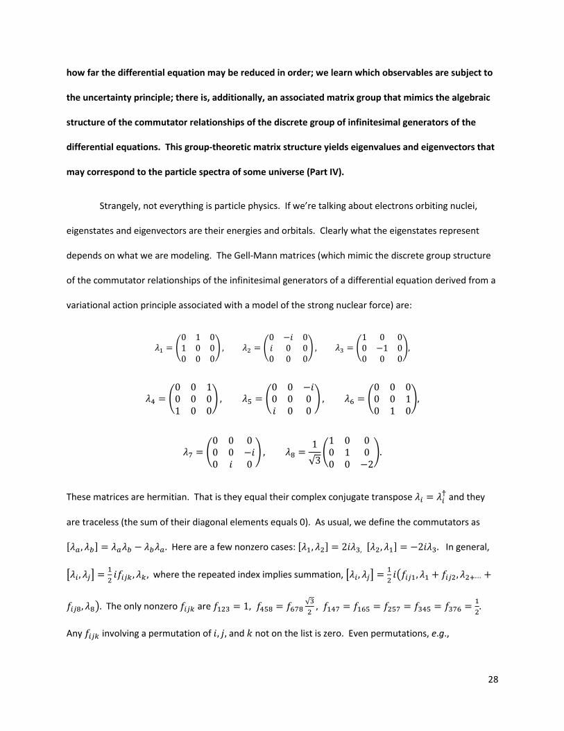
depends on what we are modeling. The Gell-Mann matrices (which mimic the discrete group structure

of the commutator relationships of the infinitesimal generators of a differential equation derived from a

variational action principle associated with a model of the strong nuclear force) are:

(

) (

) (

)

(

) (

) (

)

(

)

√ (

)

These matrices are hermitian. That is they equal their complex conjugate transpose and they

are traceless (the sum of their diagonal elements equals 0). As usual, we define the commutators as

[ ] Here are a few nonzero cases: [ ] [ ] In general,

[ ]

where the repeated index implies summation, [ ]

(

) The only nonzero are √

Any involving a permutation of and not on the list is zero. Even permutations, e.g.,

29

123312213 have the same value. The odd permutations, e.g., 123132 have opposite sign. That

is, while The symbol is said to be totally

antisymmetric in and For example, [ ]

√

(

) You may verify

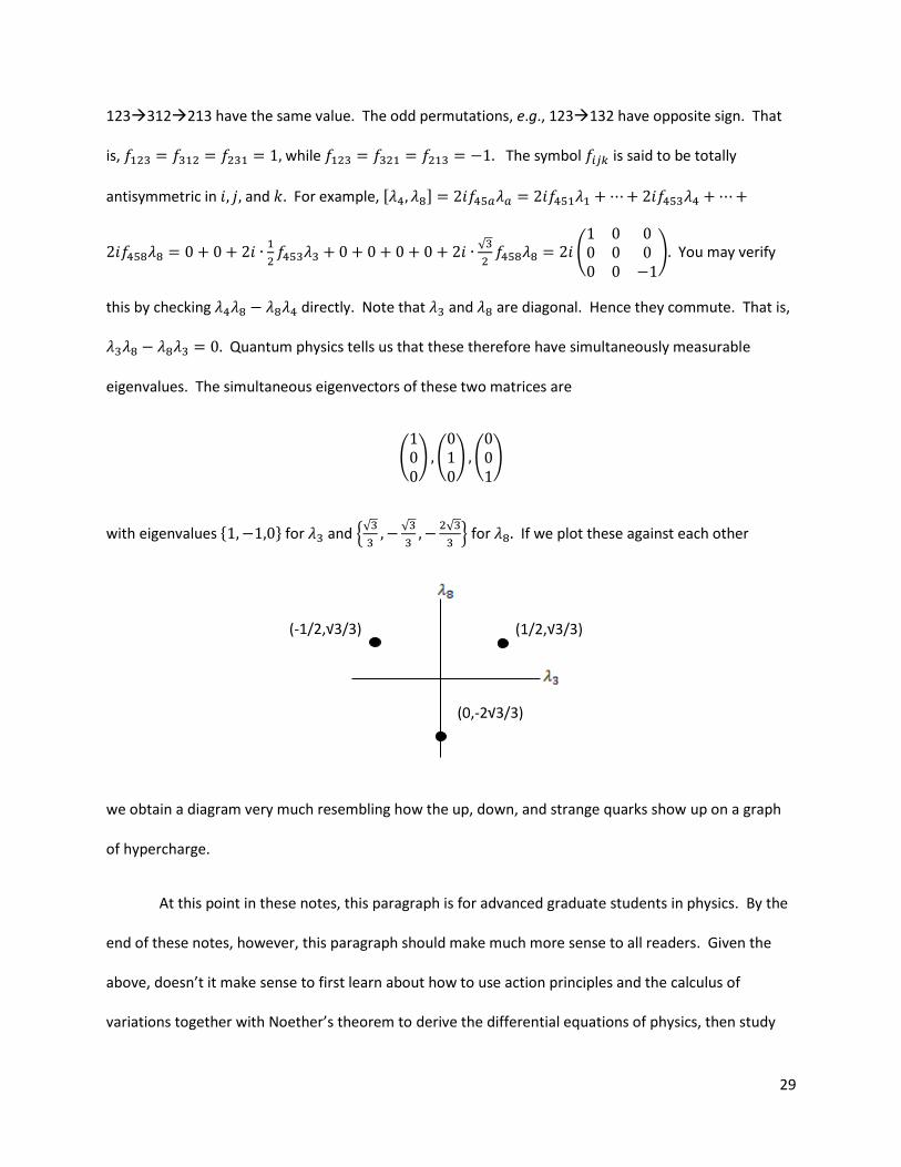
this by checking directly. Note that and are diagonal. Hence they commute. That is,

Quantum physics tells us that these therefore have simultaneously measurable

eigenvalues. The simultaneous eigenvectors of these two matrices are

( ) (

) (

)

with eigenvalues { } for and {√

√

√

} for If we plot these against each other

we obtain a diagram very much resembling how the up, down, and strange quarks show up on a graph

of hypercharge.

At this point in these notes, this paragraph is for advanced graduate students in physics. By the

end of these notes, however, this paragraph should make much more sense to all readers. Given the

above, doesn’t it make sense to first learn about how to use action principles and the calculus of

variations together with Noether’s theorem to derive the differential equations of physics, then study

(0,-2√3/3)

(1/2,√3/3) (-1/2,√3/3)

30

these differential equations using symmetry methods to find any Lie symmetries and the corresponding

discrete commutator algebra of their infinitesimal generator realizations if any? The derived subalgebra

may go down to { } under commutation as in example 1.13, or it may stop shy of { } forming

a discrete group (such as SU(2)) which can be copied by matrix representations with the same group

structure. We learn what is simultaneously measureable in terms of the eigenvalues and eigenvectors

of the representation matrices. Note that while the group may be discrete, the infinitesimal generators

themselves are continuous, the underlying Lie point symmetries being continuous groups. If the form

a linear vector space, then the local, continuous properties of these infinitesimal generators under

commutation, e.g., [ ] relate to the measure of the curvature of a space in general

relativity (in terms of the group of all coordinate transformations and connection coefficients), and

similarly to the gauge filed vector potentials in quantum field theories (in both cases in terms of the

commutators of the respective covariant derivatives). This unified overview should not take a decade to

master beyond earning a doctoral degree in physics, as it did with me. It’s physical underpinnings and

mathematical grammar should be learned by the undergraduate between the sophomore and senior

year, to be fully mastered during the first year and a half of graduate school where one should be

learning the details of advanced mechanics, electrodynamics, quantum physics, thermodynamics and

statistical physics, quantum electrodynamics, relativity, and possibly quantum fields with the power of a

unified mathematical grammar and physical overview of where shit fits together and why it fits

together. (Note—It doesn’t generally go backwards uniquely from postulating matrix representations

back to (infinitesimal generator) realizations, back to differential equations, but this is nevertheless also

a valid approach to investigate theoretical universes and extensions beyond the Standard Model.)

There is, of course, more mathematics and physics beyond the unified outline expounded on in

this work, but it ties back. For now, let’s get back to the ground. We still have to learn to crawl. After

finishing up symmetry methods for first order ODEs in chapter 1, we shall proceed to extend (or

31

“prolong”) these symmetry methods to higher order linear and nonlinear ODEs, and finally to linear and

nonlinear PDEs.

END Optional—6 Page Double Spaced “BIG PICTURE” Motivational digression Example with Discussion

Change of coordinates and the infinitesimal generator. How is the infinitesimal generator

affected by a change of coordinates? Suppose ( ) are new coordinates and let ( ) be an

arbitrary smooth function. By the chain rule

( ) ( ( ) ( )) ( ) ( )

[

] [

] [ ] [ ]

( ) ( ) ( ) ( )

Without loss of generality, since ( ) is arbitrary, in the new coordinates

( ) ( )

Thus represents the tangent vector field in all coordinate systems. If we regard { } as a basis for

the space of vector fields on the plane, is the tangent vector at ( ) The infinitesimal generator

provides a coordinate free way of characterizing the action of Lie symmetries on functions.

If ( ) ( ) are canonical coordinates, the tangent vector is ( ) and Let

( ( ) ( )) be a smooth function and ( ) ( ( ) ( )). At any invariant point

( ) the Lie symmetries map ( ) to ( ) ( ) ( ) Applying Taylor’s theorem

and given we get

( ) ∑

( )

∑

( )

32

Reverting back to ( ) coordinates, ( ) ∑

( )

If the series converges it is called the

Lie series of about ( ) We have assumed that ( ) is not an invariant point, but the expansion is

also valid at all invariant points. At an invariant point and only the term survives, which is

( ) We may express all of this in shorthand to ( ) ( ) ( )

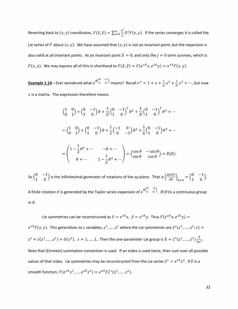
Example 1.14—Ever wondered what (

) means? Recall

, but now

is a matrix. The expression therefore means

(

) (

)

(

)

(

)

(

) (

)

(

)

(

)

(

) (

) ( )

So (

) is the infinitesimal generator of rotations of the xy-plane. That is ( ( )

)

(

)

A finite rotation is generated by the Taylor series expansion of (

). ( )is a continuous group

in

Lie symmetries can be reconstructed as Thus ( )

( ) This generalizes to L variables, where the Lie symmetries are ( )

( ) ( ) Then the one-parameter Lie group is ( )

Note that (Einstein) summation convention is used. If an index is used twice, then sum over all possible

values of that index. Lie symmetries may be reconstructed from the Lie series If is a

smooth function, ( ) ( )

33

Note that it is only sometimes easy to work from an infinitesimal generator back to a one-

parameter Lie group. Consider for example Then ( ) and ( ) Looking

at the definitions, (

)

and (

)

Thus by visual inspection and

work, and this is our Lie symmetry for our infinitesimal generator.

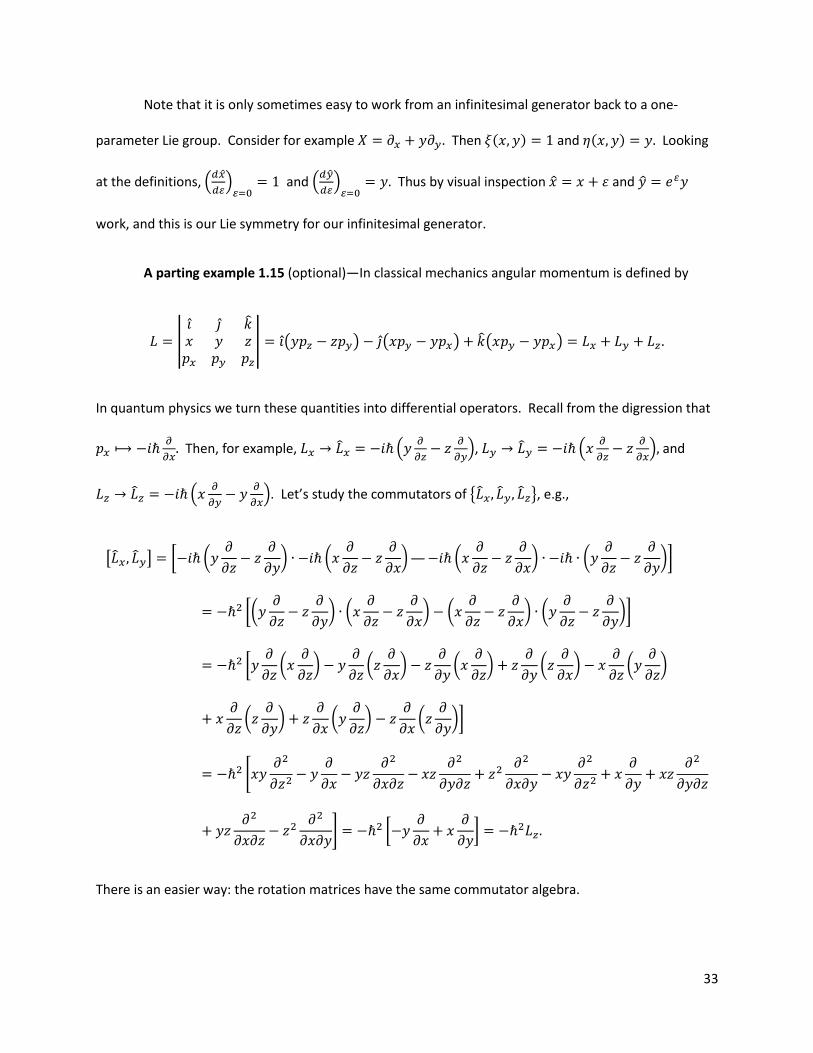
A parting example 1.15 (optional)—In classical mechanics angular momentum is defined by

|

| ( ) ( ) ( )

In quantum physics we turn these quantities into differential operators. Recall from the digression that

Then, for example, (

), (

) and

(

). Let’s study the commutators of { }, e.g.,

[ ] [ (

) (

) (

) (

)]

[(

) (

) (

) (

)]

[

(

)

(

)

(

)

(

)

(

)

(

)

(

)

(

)]

[

] [

]

There is an easier way: the rotation matrices have the same commutator algebra.

34

( ) [

] ( ) [

] ( ) [

]

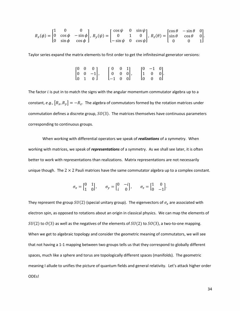
Taylor series expand the matrix elements to first order to get the infinitesimal generator versions:

[

] [

] [

]

The factor is put in to match the signs with the angular momentum commutator algebra up to a

constant, e.g., [ ] . The algebra of commutators formed by the rotation matrices under

commutation defines a discrete group, ( ). The matrices themselves have continuous parameters

corresponding to continuous groups.

When working with differential operators we speak of realizations of a symmetry. When

working with matrices, we speak of representations of a symmetry. As we shall see later, it is often

better to work with representations than realizations. Matrix representations are not necessarily

unique though. The Pauli matrices have the same commutator algebra up to a complex constant.

[

] [

] [

]

They represent the group ( ) (special unitary group). The eigenvectors of are associated with

electron spin, as opposed to rotations about an origin in classical physics. We can map the elements of

( ) to ( ) as well as the negatives of the elements of ( ) to ( ) a two-to-one mapping.

When we get to algebraic topology and consider the geometric meaning of commutators, we will see

that not having a 1-1 mapping between two groups tells us that they correspond to globally different

spaces, much like a sphere and torus are topologically different spaces (manifolds). The geometric

meaning I allude to unifies the picture of quantum fields and general relativity. Let’s attack higher order

ODEs!

35

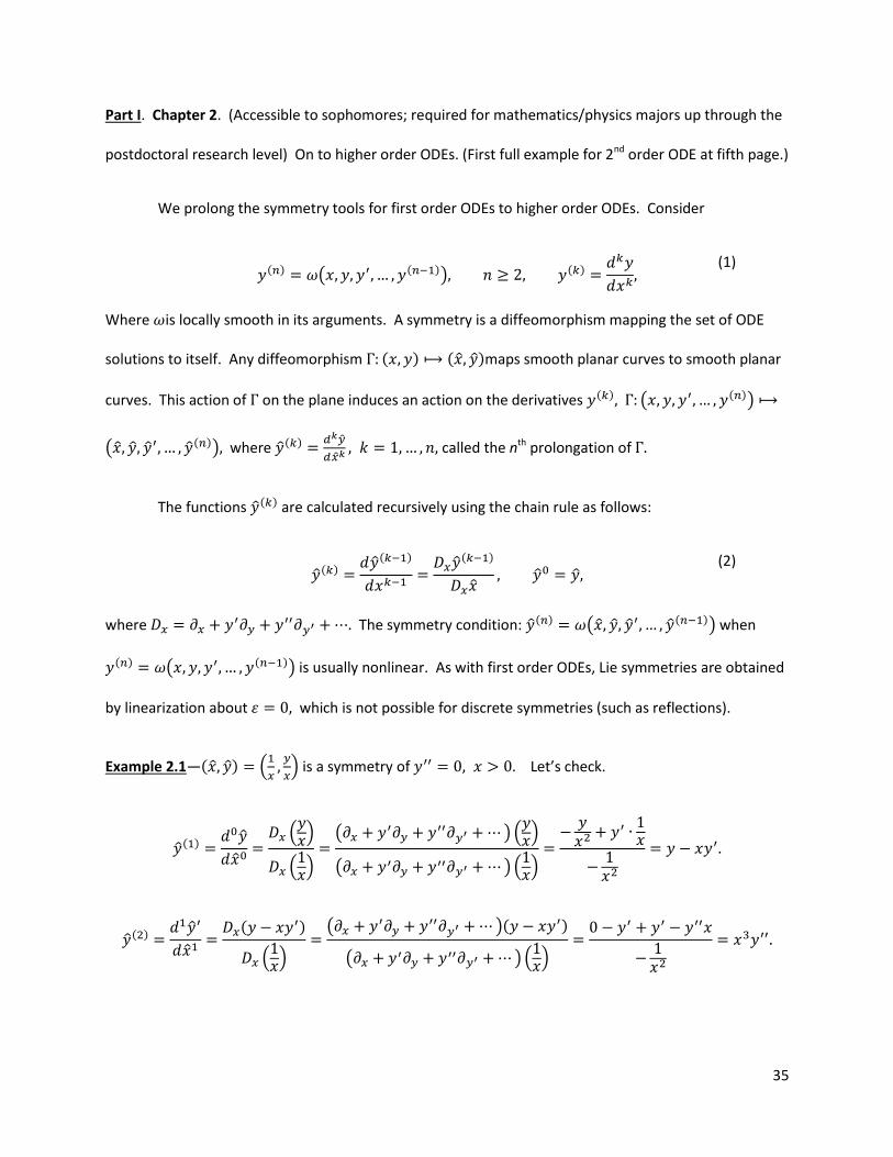
Part I. Chapter 2. (Accessible to sophomores; required for mathematics/physics majors up through the

postdoctoral research level) On to higher order ODEs. (First full example for 2nd order ODE at fifth page.)

We prolong the symmetry tools for first order ODEs to higher order ODEs. Consider

( ) ( ( )) ( )

(1)

Where is locally smooth in its arguments. A symmetry is a diffeomorphism mapping the set of ODE

solutions to itself. Any diffeomorphism ( ) ( )maps smooth planar curves to smooth planar

curves. This action of on the plane induces an action on the derivatives ( ) ( ( ))

( ( )) where ( )

called the nth prolongation of

The functions ( ) are calculated recursively using the chain rule as follows:

( )

( )

( )

(2)

where The symmetry condition: ( ) ( ( )) when

( ) ( ( )) is usually nonlinear. As with first order ODEs, Lie symmetries are obtained

by linearization about which is not possible for discrete symmetries (such as reflections).

Example 2.1—( ) (

) is a symmetry of Let’s check.

( )

( )

( )

( ) (

)

( )( )

( )

( )

( )

( )( )

( )( )

36

Therefore when The symmetry is its own inverse thus it belongs to a group of order 2.

The general solution, gets mapped to

If you have had a

little group theory you are probably familiar with the group containing { } with the binary operation

being sum modulo 1, ⟨ ⟩.

The linearized symmetry condition for Lie symmetries for higher order ODEs is derived by the

same method used for first order ODEs. Given an ansatz symmetry ( ) ( ) the trivial

symmetry corresponds to The prolonged Lie symmetries are of the form

( )

( ) (3)

( ) ( ) ( ) ( )

Where The superscript ( ) is merely an index. Substitute (2) into ( ) ( ( ))

( ( )) ( ( ) ( ) ( ) ( ) ( )

( ) ( )) [ ] [ ( ) ( ) ( )]

where the linearized symmetry condition for an nth order ODE is

( ) ( ) ( ) ( ) (4)

We find the ( ) recursively from (2). Recall

for small . Consider the case for

( )

( )

( )

( )

( )

( )

( ( ))

( )

( )

( ) ( )( ) ( )

( ) ( )

37

So,

( ) ( ) (5)

Then continuing on to the kth step, we have

( )

( ) ( ) ( )

( )

( ( ) ( ))(

( )) ( )

(6)

Thus,

( )( ) ( ( ) ( ) ) (7)

Mimicking the notation of chapter 1, we may write this in terms of the characteristic by

letting ( ) ( )

Recall that for first order ODEs the RHS of the linearized symmetry condition is

and the tangent vector to the orbit through ( ) is ( ) (

)

For nth order ODEs we

have

( ) ( ) ( ) ( ) (8)

defining the prolonged infinitesimal generator. Thus ( ) is associated with the tangent vector of the

space variables ( ( )) So far every symmetry we have met is a diffeomorphism of the form

( ) ( ( ) ( )) which we call a point transformation. Any point transformation that is a

symmetry is point symmetry. Let us stick with point symmetries until further notice. Then for point

symmetries we have ( ) and ( ) only. These components of the tangent vector do not

depend on . Assuming that we have our symmetry ( ) ( ( ) ( )) and the

corresponding tangent vector ( ) let’s make the first few cases of equation (7) explicit, say for

For

38

( )

( )

( )

( )

(9)

For

( ) ( )

( )( ( )

)

( )

( ) ( )

( )

(10)

For

( ) ( ) ( )

( )

( ( )

)

(

)

(11)

It gets increasingly monotonous. To keep things manageable and clear, let’s consider second-order

ODEs of the form ( ) The linearized symmetry condition is obtained by substituting ( )

into ( ) ( ) and then replacing by ( ) We get

( ) ( ) ( )

(

) ( )

( ) ( ( )

)

39

Though the equation looks complicated, it is often easy to solve. As both and are independent of

we may decompose the linearized symmetry condition into a system of partial differential equations

(PDEs), which are the determining equations for the Lie point symmetries.

Example 2.2—Consider Our goal is to find a Lie point symmetry. Yes we are going overboard

with a very simple 2nd order ODE, but what we learn will greatly simplify not-so-simple 2nd order (and

higher order) linear and nonlinear ODEs (see next example). Note

Thus ( ) simplifies to ( ) ( )

As both and are

independent of the linearized symmetry condition splits into the following system of determining

equations:

The general solution for is ( ) ( ) ( ) Take two partial derivatives wrt to to

verify that indeed Now consider the third equation Then

[ ( ) ( )]

( ) ( )

Integrating twice we get ( ) ( ) ( ) Then ( ) ( ) ( ) and

( ) ( ) ( ) (12)

What is ? First ( ) ( ) then ( ) ( ) Then the second equation tells

us ( ) ( ) On the LHS, ( ( ) ( )) So with LHS = RHS we get:

( ) ( ) ( ) (13)

If in (12), then ( ) and ( ) and ( ) Ditto if in (13) then ( )

and therefore ( ) ( ). Integrating ( ) gives us ( ) Integrating

( ) gives ( ) Therefore, ( ) ( ) Integrating ( ) once we get

40

( ) One more integration gets us: ( ) . Repeating for ( )

we get ( ) Thus our Lie point symmetry is

( ) ( ) ( )

( ) ( ) ( ) ( ) ( )

Let’s re-label the Greek indices with Arabic numerals: Then ( )

and ( ) Now

( ) ( ) ( ) ( )

( ) (

)

The most general infinitesimal generator is ∑ where

Example 2.3—Consider the nonlinear ODE

Recall the linearized symmetry condition

( ) ( ) ( )

(

) ( )

( ) ( ( )

)

The term ( ) is the RHS of our nonlinear ODE. The term is zero. The term is

The term is ⁄ Thus for our nonlinear ODE our linearized symmetry condition is

( ) ( )

{

} (

)

(

) ( ( )

) (

)

41

We proceed as before by matching powers. Matching powers of leads to the determining equations

(14)

(15)

(16)

( ) (17)

Abusing notation, let’s integrate the first of these equations

∫

∫

We get ( ) where ( ) is some arbitrary function of This can be rewritten as

| ( )| So, ( ( ) ) ⁄ Integrating again gives us ( ( )⁄ ) | | ( ) where

( ) is another arbitrary function of Let ( )⁄ ( ) Then

( ) | | ( ) (18)

You can check this by taking Integrating the second of the equations yields

( ) ( | |) ( ) | | ( ) (19)

where, as usual, the functions of are arbitrary. Substituting (18) and (19) into (16) results in

( ) | | ( ) ( ) ( ) (20)

If then

( ) ( ) ( ) (21)

Substituting (18) and (19) into (17) results in (remembering ( ) )

( ) | | ( ) ( ( ) ( ) ( ) ) ( )

42

which splits into the system

( ) ( ) ( ) ( )

Taking into account equations (21), we see that

( ) ( )

where the constants and are arbitrary. Hence the general solution of the generalized symmetry

condition is ( ) ( )

I’ll bet that when I said symmetry methods for solving differential equations are based on

making good guesses on symmetries, you thought that symmetry methods are just as full of crap as

anything else. Maybe only a genius could cook up a symmetry for the Riccati equation. Not so. In this

example we began with an ugly, nonlinear, 2nd order ODE and through the machinery of symmetry

methods produced the tangent vector ( ) to a symmetry of our ugly ODE. It may not be easy to work

from the tangent vector back to the symmetry, but the tangent vector hasn’t yet been fully exploited.

Recall that our goal is to find solutions to our ODE.

Let’s use our two infinitesimal generators to look directly for possible invariant solutions from

the characteristic equation for each generator. Recall from chapter 1 that every curve on the -

plane that is invariant under the group generated by a particular satisfies the characteristic equation:

( ) on Let’s try it for We know and thus for and

Thus for the characteristic equation is The solution to this characteristic

equation is where is an arbitrary constant. If you plug in this possible solution into the ugly ODE

it works. So is a confirmed solution. Now for our second characteristic equation for . Here

and hence we determine when The solution to this simple ODE is

⁄ where is an arbitrary constant. Is this solution a solution to our nonlinear ODE? Plug in

43

and check. First let’s compute the derivatives:

Plug these into

to get

This simplifies to or Thus ⁄ is a solution. Check it:

(

)

Not bad. Be careful. For linear ODEs the sum of solutions is a solution. This is not generally so for

nonlinear differential equations. We have found two distinct solutions: and ⁄

Get ready for some excitement—the useful union of abstract algebra to differential equations.

We will reduce our ODE down to an equivalent algebraic equation. Let’s first check if the algebra of the

infinitesimal generators of our ODE is solvable. That is, let’s check to see whether { } { }

or not under commutation. Well,

[ ] ( ) ( )

Since [ ] { } { } { }. To go from { } to { } requires two steps. Thus our

2nd order ODE can (at least in principle) be integrated twice via differential invariants/canonical

coordinates. [I owe you a proof of this, and you will get it.] One technique for reducing the order of a

differential equation is the reduction of order using canonical coordinates. We’ve used canonical

coordinates already for solving an example in chapter 1. Another technique involves computing

differential invariants (this approach will be presented after canonical coordinates). When the algebra is

solvable, we get the best of these approaches.

44

Since we have used canonical coordinates before, let’s use them to reduce the order of our 2nd

order ODE down to first order. Actually, you’ll see that we can reduce our particular 2nd order ODE to

two distinct 1st order ODEs depending on our choice of canonical coordinates. Recall that we can use

canonical coordinates when the ODE has Lie symmetries equivalent to a translation, e.g., ( )

( ) For we have and , so (chapter 1) ( ) (∫

( ( ))) ( )

∫

and

( )

( )

Thus So our canonical coordinates are

( ) ( ) Then

and

and so

⁄ ⁄

Let

With

and

we get

Dividing our ODE by and rearranging terms we get to

Combining the two result above gives us the following first order ODE:

On the other hand, if we let

then

and with

we get

I suppose which choice of is better is the one that produces the easier reduced ODE to work with.

Regardless, we have reduced a 2nd order ODE into one or another first order ODE, but according to the

45

fact that we have two Lie point symmetries, we can transform our 2nd order ODE down to an algebra

equation. Although we will need to build more machinery to more systematically reduce ODEs to lower

order you have enough background to peek ahead and see how to take our particular 2nd order ODE

down to an algebra equation. You’ll have to take one result on my word until we build up this math.

So far we have only used the first infinitesimal generator of our 2nd order ODE. Let’s

proceed to use the second infinitesimal generator To keep things clear we will use

subscripts. Corresponding to generator we have canonical coordinates ( ) ( ) Using the

subscript 2 for we have and , and equation (8) reduces to

( ) ( ) (22)

The method of characteristics tells us

( )

(23)

What is ( )? Equation 9 tells us that

( )

( )

This reduces to ( ) ( ) So equation (23) becomes

(24)

Let’s work with the last two terms. Integrating the last two terms gives

Thus

Until I cover the material for differential invariants you will have to take my word that:

(see example 2.7). Our canonical coordinates are ( ) Notice that if I rearrange the

original ODE to match

we get

and there you have it. A

46

second order ODE turned into an algebraic equation. Since we’re not interested in voodoo, here is

what I owe you: the theory of differential invariants to get to

I also owe you the connection

between the solvability of the Lie algebra, { } { } { } and the ability to integrate our

2nd order ODE stepwise by two integrations. We will get here soon. We will do so for our particular

example, taking it to completion, and we will do so in general for any ODE and its Lie algebra.

It’s remarkable how we’ve treated our 2nd order ODE by assuming that at least one Lie point

symmetry exists and using the linearize symmetry conditions to get tangent vectors to the Lie

symmetries, to get some invariant solutions, to get the infinitesimal generators and , to get

canonical coordinates, to reduce our ODE down to two different first order ODEs [no voodoo through

here], and finally reduce the 2nd order ODE down to a polynomial. Let’s do two more examples of

reduction of order using canonical coordinates before formalizing the examples into our grammar

afterwards.

Example 2.4—Consider the 2nd order ODE (

)

Since I did every step in using the linearized symmetry condition, I will forego all of that here and state

that one of the infinitesimal generators is So for this generator and Given this,

we may derive the canonical coordinates ( ) ( | |) We have seen these before. Then we get

We are clearly aiming to reduce the order of our ODE from two to one. When we “prolong” we get

47

So

If we divide our ODE by we get

(

)

Combining the two above equations gets us

(

)

Thus, again, we arrive at a first order equation (in this case a Riccati equation):

(

)

Wikipedia writes a general Riccati equation as ( ) ( ) ( )

Example 2.5—Being a little adventuresome. Consider

(

)

Again, exploiting the linearized symmetry condition, we can determine that one of the infinitesimal

generators is (These translations are the only Lie point symmetries of our ODE.) Since

and =0 we get canonical coordinates ( ) ( ) With

and

, let

⁄

⁄

With

and

we get

Then

48

(

)

(

)

This is a Bernoulli equation whose solution is given in the typical botany-based class in ODEs. What if

instead of choosing

we choose Then ⁄ and ⁄ Then

(

)

(

)

The result is a linear ODE, yet another of the ODEs studied in a regular, botany-based ODE class.

¿Botany? Ha! We don’t need no stinckin’ botany. Vamonos!

So far we have been able to reduce the order of our 2nd order ODEs by one because each of the

these 2nd order ODEs have had at least one Lie point symmetry, and therefore one corresponding

infinitesimal generator extracted from the linearized symmetry conditions. We don’t need the actual Lie

point symmetries because we extract what we need from the tangent vectors of these Lie point

symmetries which we get from the linearized symmetry condition. Some of our ODEs have actually had

two infinitesimal generators extracted from the linearized symmetry conditions, and in some cases

these pairs of generators have formed a solvable Lie algebra. For these 2nd order ODEs with solvable

algebras I have claimed that we can integrate them stepwise two times. We haven’t bothered to do this

for the prior two examples because the reduced 1st order ODEs we have arrived at are straightforward

1st order ODEs that we can readily solve. Let’s formalize this machinery of reducing the order of an ODE

by using canonical coordinates. Then we will go over an example reducing a 3rd order ODE down to a 1st

order ODE. Ultimately we will use stronger machinery to more fully treat example 2.3. What follows is

the formalization of the reduction of order technique we used in examples 2.4 and 2.5 using canonical

coordinates.

49

Reduction of order by using canonical coordinates: From now on we shall denote differentiation

by by a dot ( ). For example, denotes ⁄ Suppose that is an infinitesimal generator of a one-

parameter Lie group of symmetries of ODE

( ) ( ( )) (22)

Let ( ) be canonical coordinates for the group generated by so that If ODE (22) is written

in terms of canonical coordinates, it is of the form

( ) ( ( )) ( )

(23)

for some However, ODE (23) is invariant under the Lie group of translations in so the symmetry

condition gives Therefore

( ) ( ( )) ( )

(24)

By writing ODE (22) in terms of canonical coordinates, we have reduced it to an ODE of order for

This is just what I did in example 2.3 just south of equation (24). So with ,

( ) ( ( )) ( )

(25)

Suppose (assume) that the reduced ODE has general solution

( )

Then the general solution of ODE (22) is arrived at by integration,

( ) ∫ ( ) ( )

More generally, if is any function of { } so that ( ) then(24) reduces to form

50

( ) ( ( )) ( )

(26)

Once the solution of (26) is known, the relationship ( ) gives the general solution of (22):

( ) ∫ ( ( )

( )

(27)

In summary, once we find a one-parameter Lie group of symmetries using whatever means (say a good

guess) or the tangent vectors to any such one-parameter Lie group via the linearized symmetry

conditions), we can solve ODE (22) by solving a lower-order ODE, then integrating. This is what we have

done in examples 2.3 through 2.5.

On Differential Invariants and Reduction of Order: In just about as much theory of the previous

section we will have the differential invariants method to reduce the order of a differential equation.

We have seen that a single Lie point symmetry allows us to reduce the order of an ODE by one.

Sometimes a double reduction of order can happen if there are two Lie point symmetries. In fact one

can reduce an nth order ODE with Lie point symmetries to an ODE of order or to an

algebraic equation if

If generates Lie point symmetries of the ODE

( ) ( ( )) (28)

then, in terms of canonical coordinates ( ) the ODE reduces to

( ) ( ( )) (29)

Where ( ) is any function such that The reduced ODE consists entirely of functions that

are invariant under the (prolonged) action of the group generated by These functions are called

differential invariants. A nonconstant function ( ( )) is a kth order differential invariant of

the group generated by if

51

( ) (29)

In canonical coordinates, ( ) so that every kth order differential invariant is of the form

( ( )) or equivalently,

( ( )) (30)

for some function The invariant canonical coordinate ( )is the only differential invariant of order

zero (up to function dependence). All first-order differential invariants are functions of ( ) and

( ) Furthermore, all differential invariants of order two or greater are functions of and

derivatives of wrt Therefore, and are called fundamental differential invariants. We can usually

find a pair of fundamental differential invariants without first having to determine From equation

(29), every kth order differential invariant satisfies ( ) ( )

so (by the method of characteristics), I is a first integral of

( )

( )

(31)

In particular, is a first integral of

and is a first integral of

( ) Sometimes it is

necessary to use to obtain

Example 2.6—Find fundamental differential invariants of the group of rotations generated by

Thus and Then

Solving this simple ODE leads to

I let the constant be because the left hand side is the equation of a circle.

Then √ Note that ( )√ That is We already know

that is a first integral of

. Now on to . It is the first integral of

( ). Well

( ) ( )

So is a first integral of

52

To keep things simple we restrict attention to the region where

√ . Note that

∫

and ∫

∫

√

So

Then the first integrals are of the form (

) Since

is

constant so is (

)

by identity. Then it’s convenient to let

What is ? By definition,

( ) (∫

( ( ))) ( )

∫

∫

√

Let’s compute , or

.

(

)

( )

( )

⁄

√ ( )

( )

Notice that We can think of as angular velocity and as the tangential velocity.

An ODE that has more than one Lie point symmetry can be written in terms of the differential

invariants of each generator. Thus the generators themselves can be written in terms of functions that

are invariant under all of its symmetries. Let denote the set of all infinitesimal generators of one-

parameter Lie groups (the binary operation being commutation) of point symmetries of an ODE of order

The linearized symmetry condition is linear in and by construction, and so

53

Where { } is a basis for . The set of point symmetries generated by all forms an -

parameter (local) Lie group called the group generated by (The order of an ODE places restrictions on

For 2nd order ODEs, iff the ODE is linear, or is linearizable by a point

transformation. Every ODE of order has If this ODE is linear or linearizable, then

{ }. These results have been offered without proof.)

Because { } is a basis for , the fundamental differential invariants of the group

generated by are solutions of the system

[

( )

( )

( )

( )

( )

( )]

[

( )]

[

]

(32)

(A good example is coming up.) The system has two functionally independent solutions if the matrix on

the LHS has rank These solutions can be determined via Gaussian elimination and the methods of

characteristics. One solution is independent of ( ) and is denoted by We denote the other solution

which depends nontrivially on ( ) As

⁄ depends on ( ) and so on, ODE (22) reduces to

( )

( ( ))

( )

for some function Thus an - parameter symmetry group enables us to reduce the order of the ODE

by

Example 2.7—Consider ( )

( ) Is this ugly enough for you? As in example 2.3, you

would apply the linearized symmetry condition to find ( ) ( ) From these we would find the

infinitesimal generators. Recall example 2.3. There we got ( ) ( )

54

Thus there were two constants in that example, and (if you go back) we had two infinitesimal

generators, namely, and Doing this math for our 4th order ODE you get:

(33)

So , and for ( )

( )

( )

For ( )

( )

( ) The result for ( ) follows from substituting and into (9):

( )

( ) ( )

The result for ( )

results from substituting and ( )

into equation (10)

( )

( ) ( ) (

)

( ) ( ) ( )

The result for ( ) results from substituting

( ) into equation (11) to get (you do the math)

( ) For the third index and Repeating the use of equations (9), (10) and

(11) gives us ( )

( ) ( ) and ( ) Thus we get

[

( ) ]

[

]

[ ]

After Gaussian elimination we get

[

]

[

]

[ ]

(34)

55

So ( ) Now use each equation of (34) to determine the differential invariants. The

third equation is

Using the method of characteristics we get

Solving this leads to ∫ ∫ , or,

Since is constant, it is one of our differential invariants. So

( )

The second equation from (34) is

The method of characteristics gives us

Integrating the first and third terms

or ⁄ So is constant.

( ) ( )

We’ve eliminated The third equation is or via the method of characteristics ⁄ Then

Therefore ( ) So the fundamental differential invariants of the group

generated by our generators (33) are Higher order differential

invariants can now be computed, say ⁄

( ( ) )

( ( ) )

( )

( )

( )

56

Note that our ODE ( )

( ) when rearranged is

( )

(a differential

invariant). Solving

gives us

The ODE has been turned in the algebra equation equivalent to a 3rd order ODE, namely,

This 3rd order ODE is invariant under the three parameter Lie group generated by By the way, I have

now showed you the method by which I got

back in example 2.3.

Of course we can proceed backwards. A set of fundamental differential invariants can be used

to construct ODEs that have given Lie point symmetries. If ( ) are fundamental differential

invariants of an - dimensional Lie group then every ODE (28) of order that has as its

symmetry group can be written in the form

( )

( ( )) (35)

for some function . By expressing (35) in terms of ( ( )) one obtains a family of ODEs that

have the desired symmetries. Some of these ODEs may have extra symmetries. Let’s quickly see how

this “going backwards” idea works. After this we finally get to the solvability theory.

Example 2.8—Suppose that the fundamental differential invariants of the three-parameter group

generated by are ⁄ The most general third-

order ODE with these symmetries is ( ), which is equivalent to ( ). The most

general fourth-order ODE with these symmetries is equivalent to ( ) ⁄ First let’s

compute ⁄ We get ⁄ Now let’s compute ⁄ We get

57

( )

So then

( )

( )

(

)

Thus

( )

( )

As they say in today’s Air Force, the bottom line up front (BLUF) is: If an ODE has Lie

point symmetries, we can reduce its order from to If , and if the algebra is solvable

then (at least in principle if the manipulations are doable) we may, additionally, integrate the ODE

times to solve it. This is a theorem. It requires proof, which requires some more foundations. Please

skim the rest of this chapter at a minimum for now if you’ve just finished a sophomore course in ODEs

and you wish to keep going with applications to ODEs and PDEs in chapter 3. The rest of this material is

IMPORTANT if you are beginning graduate studies in physics so that you better understand the

mathematical engine underlying quantum physics, or if you’re either planning or are already doing work

in particles and fields, even as a post-doctoral research fellow. The material here on the classification of

symmetries is well developed via realizations versus the pedagogical half picture via matrix

representations. Of course I will include examples, and I will try to highlight the important stuff in bold.

DON’T let the upcoming theory derail you from the momentum you have in applying symmetry

methods for ODEs. DON’T worry about totally mastering the following theoretical material until you

have the practical methods down pat. Lie point symmetries ARE NOT the only symmetries we can

exploit regarding differential equations. We’ll meet some of these other symmetries in this chapter.

58

Proof Section to Theorem (Some grammar/theory first)—If , and if the algebra is

solvable then (at least in principle) we may integrate the ODE times to solve our ODE. Let’s suppose

that the Lie point symmetries of ODE

( ) ( ( )) (1)

are generated by which is -dimensional. We know (and we have seen from several examples) that

we may rewrite ODE (1) in terms of differential invariants ( ) to obtain an ODE reduced down to

order leaving us with an algebraic equation,

( )

which is equivalent to an ODE of order with the -parameter group of symmetries generated by

To answer our theorem we need to learn more about the structure of (stuff that is very important to

graduate students of physics).

Suppose that where

( ) ( ) (36)

The product is a second-order partial differential operator:

( )

( ) ( )

where the last two terms have come from the chain rule. The product has the same 2nd order

terms as , but first order terms (from the chain rule) of ( ) ( ) . So the commutator

[ ]

( ) ( )

(37)

The commutator has many useful properties. Here are a few. It is antisymmetric: [ ] [ ]

The commutator satisfies the Jacobi identity

59

[ [ ]] [ [ ]] [ [ ]]

The commutator is bilinear, i.e., linear in both arguments:

[ ] [ ] [ ]

[ ] [ ] [ ]

where the are arbitrary constants.

The Lie algebra is invariant under a change of variables. Let’s check this. Under a change of

coordinates from ( ) to ( ) each generator transforms according to the chain rule. Let’s find

out how this affects the commutator. Let [ ]; the new accent mark is being used for writing

the various in terms of the new coordinates ( ) That is in new coordinates ( ) we have

( ) ( )

Let ( ) be an arbitrary function. Then it must be that

[ ] {( ) ( ) } {( ) ( ) }

( ) ( ) ( ) ( ) ([ ] ) ([ ] )

( ) ( )

However, since is an arbitrary function (meaning the results don’t depend on ) we conclude that

[ ] ( ) ( )

The commutator is therefore independent of the coordinate system in which it is being computed. We

don’t have to distinguish between and

All of the commuter properties that we have discussed so far have been in terms of

commutators acting on the plane. The commutators of the prolonged generators

60

( )

( ) ( ) ( )

Is defined similarly: [ ( )

( )

] ( )

( )

( )

( )

Without loss of generality suppose, for example, that ( ) ( )

(Recall that our choice of coordinates does not affect the commutator.) Then

[ ] ( ( ) ( ) ) ( ( ) ( ) )

From the beginning of the chapter, ( ) ( ), the prolongation formula for ( )

is

( ) ( )

Plugging in to [ ( )

( )

] we get

[ ( )

( )] [ ( ) ] ( ( ) ) ( ( ) )

( )

( )

( )

(In a different approach we could have used the fact that and commute ( (

) ( ) ) Thus [ ] and [ ( )

( )]

( )

The result continues for all For note that ( ) ( ) (

( )

( ) ) ( )

, these relationships having been developed in earlier parts of this chapter. Thus

[ ( )

( )

] ( )

in any coordinate system.

Now we show that if then [ ] otherwise known as closure. With ( )

( )

( ) ( ) we have that ( )

( ) ( ) all other terms but the last

61

term being zero. Then ( )

( ( ) ) ( )

( ) when ( ) For the

prolongation formula implies that ( )is linear in the highest derivative, ( ) whereas and therefore

( )

are independent of the ( ). The linearized symmetry condition thus implies that ( )

( ( )

) ( ( ) ) where (

( ))

( )

( ) Let [ ] Now consider ( )( ( )

) [ ( )

( )

] ( ( ) ) ( )

( )

( ( ) ) ( )

( )

( ( ) ) ( )

( ( )

( ( )

)) ( )

( ( )

( ( ) )) ( )

( ( ) )

( ) (

( ) ) ( ( )

( )

) ( ( )

) Hence ( )( ( ) ) when ( ) and therefore generates Lie point symmetries.

The same holds for the case for , but it’s complicated by the fact that ( ) is quadratic in

Recall: ( ) ( )

So, if then [ ] (closure).

Important (physics) definitions. For the set is a finite-dimensional vector space. Once

we pick a basis { } for every generator of Lie point symmetries can be written as a linear

combination of the generators in the chosen basis: [ ] where the

are called the

structure constants. If [ ] the generators and are said to commute. Clearly, every

generator commutes with itself. Particle physicists deal with structure constants all the time, but they

deal primarily with matrix representations of a Lie algebra, not with realizations of the infinitesimal

generators as we’re doing. Now let’s get this out of the way. A vector space is defined to have certain

properties which you can readily look up. If a vector space also has a product (in this case our

commutator “product” [ ] , then this vector space is a Lie algebra. A Lie algebra is a vector

space that is closed under commutation where commutation is bilinear, antisymmetric, and satisfies the

Jacobi identity. Antisymmetric means [ ] [ ] which implies

Evidently so

we only compute the generators with The Jacobi identity [ [ ]] [ [ ]]

[ [ ]] . It is true iff

62

Example 2.9—The Lie algebra of Lie point symmetries of is two-dimensional, being spanned

by the basis

Then [ ] (

) (

)

Now [ ]=[ ] and [ ] Thus the

only nonzero structure constants for the basis are and

Example 2.10—In the last example of chapter 1 (Example 1.15) I introduced you to the three-

dimensional rotation matrices defining the group ( ), the rotation matrices providing the matrix

representation of the ( ). The three matrices form the basis of ( ). The realization of ( )

came from the basis of quantum mechanical angular momentum operators derived from converting

their classical mechanics versions to their quantum mechanical versions. The basis for a representation

or realization of ( ) are not unique. Here is another representation with basis

( ) ( ) ( )

such that The only nonzero structure constants are

(The structure constants are unchanged by a cyclic permutation of the indices (123).) The Lie algebra

with these structure constants is ( ). The Lie group generated by ( ) is ( ), the special

orthogonal group. An alternative realization in terms of generators of Lie point symmetries is

( )

( )

It follows from previous results that structure constants are unaffected by a change of variables

or prolongation. HOWEVER, structure constants depend on the choice of basis for Life is easier in a

basis with as few nonzero structure constants as possible. (This reminds me of Gram-Schmidt

orthonormalization process.) If all the basis vectors of the basis commute, the Lie algebra is abelian.

63

Example 2.11—(A practice problem) Consider the most general two-dimensional Lie algebra with basis

{ } The commutator of with is of the form [ ]

The Lie algebra is

abelian iff

This is also the condition for linear independence: are linearly

independent if is the only way to make . If the Lie algebra is not abelian we

can find another basis [ ] such that [ ] (We have shown that our algebra is

independent of our coordinate basis, so if [ ] then [ ] ) To compute this other

basis, note that the commutator of any two generators must be a multiple of

the most

general commutator by our construction for and . Let

Suppose then

[ ] [

] [ ]

[ ] [ ]

[ ]

which is off by a factor of To fix this, let

Similarly if

but the Lie algebra is non-

abelian, then letting

would satisfy our [ ] Let’s check.

[ ] [

]

[

]

[ ]

Vector spaces can be built from vector subspaces in various ways and Lie algebras may be built

from Lie subalgebras. How we join the Lie subalgebras determines the structure constants of our Lie

algebra. Let [ ] be the set of all commutators of generators in with generators ,

that is, [ ] {[ ] } A subspace is a subalgebra of a Lie algebra if it’s

closed under commutation, [ ] A subalgebra is an ideal if [ ] . The set { }

and are both, trivially, subalgebras and ideals. Any other ideal other than the trivial ideal is a proper

ideal. Facts: every one-dimensional subspace of is a subalgebra but not necessarily an ideal as each

commutator commutes with itself. Almost all Lie algebras of dimension have at least one two-

dimensional subalgebra; the one exception (important to physics) is the simple Lie algebra ( )

64

Example 2.12—(Another Lie algebra important for physics ( ) Given the three-dimensional Lie

algebra The nontrivial (nonzero) commutators of [ ] are

[ ] [ ] [ ]

This Lie algebra is the special linear group ( ) which generates ( ) The subalgebras are

Span( ) and Span( ), which are two-dimensional. Span( ) is not closed. Hence it’s not a

subalgebra. The group ( ) has only the trivial ideals. Note—In later work we use groups (with only

one binary operation) to study structure constants versus ideals (with two binary operations).

Important: Given any Lie algebra , one ideal that can always be constructed is the derived

subalgebra ( ) which is defined by ( ) [ ] Of course [ ( ) ] ( ), making ( ) an ideal of

If ( ) we may continue to find the derived subalgebra of ( ) via ( ) [ ( ) ( )], … ,

( ) [ ( ) ( )] until we obtain no new subalgebra. If for some we get ( ) { }, then is

said to be solvable. Given point symmetries of and ODE, an -dimensional Lie algebra is solvable if

there is a chain subalgebras such that { } where ( ) such that

is an ideal of for each Seen from several previous examples we now see any non-abelian

two-dimensional Lie algebra has a basis such that [ ] and hence is solvable. For each

there exit lie algebras that are not solvable, e.g., ( ).

Important: Given an -dimensional solvable Lie algebra, it’s best to choose a basis such that

Hence ( ) This basis is the canonical basis. Equivalently, a basis is canonical if

65

Example 1.13—Recall this example? Given ( )

the linearized symmetry condition leads to the

following set of infinitesimal generators: leading

to a five-dimensional Lie algebra { } From all possible commutators taken from the

set { } we only get back the infinitesimal generators { } There is no

[ ] where is nonzero. We say that the infinitesimal generators { } form a

derived subalgebra ( ) ( ) under the (binary) operation of commutation. Now by

taking all possible commutators from the set { } you only get back two infinitesimal

generators, namely, ( ) { }. Repeating this using all possible commutators from { }

you get ( ) { } We conclude that is solvable.

Finally we get to stepwise integration of ODEs (as to when this is possible at least in principle).

We know that given and ODE of order that has an -dimensional Lie algebra we may rewrite the

ODE in terms of differential invariants as

( )

for some function When can we solve the ODE by using each symmetry generator in turn? (As we

proceed, we assume that generators are sufficiently prolonged to describe the linearized group action

on all variables.)

Suppose that the generators form a subalgebra of . Let ( ) be the

fundamental differential invariants of this subalgebra. If the remaining generator acts on

( ) as a generator of point transformations, there exist canonical coordinates

( ) ( ( ) ( ))

66

as every noninvariant “point” in terms of which (We can find ( ) by methods we’ve done

in the examples.) The is a function of and ( ) for some function Hence we obtain

( ) ∫ ( ) ( )

which is invariant under the group generated by If this equation can be solved for

we get a problem of the form ( ) Provided we can iterate this procedure sufficiently many

times, we will obtain the general solution of the ODE. This is so iff is solvable.

Proof: Clearly acts on ( ) as a generator of point transformations if the

restriction of to the variables ( ) is of the form

( ) ( )

for some functions at least one of which is nonzero. Thus we require that

( ) ( )

The differential invariants satisfy

and hence

[ ] ( )

We may rewrite this as

leading to

( )

67

By a similar argument, [ ] leads to

( )

Therefore, since at least one is nonzero,

Span( ) is a subalgebra if

So acts as a generator of point transformations on ( ) iff

This condition enables us to reduce the order once. Similarly, a second reduction of order is possible if

Continuing in this way, each generator may be used to carry out one integration if

This is only satisfied (in any canonical basis iff is solvable. This also works for provided that

has an -dimensional solvable algebra (see Hydon text chapter 6 for examples).

IMPORTANT: The following material is on the classification of invariant solutions and the

classification of discrete symmetries. The latter material (which you should at least peruse if you’re

pressing on to working more PDEs with symmetry methods) is of foundational importance to students of

particles and fields, which is typically presented to students without any connection to differential

equations, and usually by uninformed lecturers and dismal, dry, confusing books. In this section you will

68

with study the classification of invariant solutions and the classification of discrete symmetries in terms

of realizations. Several chapters further on will carefully build up the parallel material in terms of matrix

representations with, naturally, plenty of step-by-step examples. I don’t think that one can be a

complete physicist, applied or theoretical, without this much broader picture of symmetry methods.

This stuff underlies many of the “invariants” that are just given to you in text books and by lecturers. It

also underlies the very mathematics that you will use during your one year studies in graduate quantum

physics, not to mention quantum field theories. The applications of these methods, in fact, go to all

physics.

On the Classification of Invariant Solutions. Two invariant solutions are equivalent if one can

be mapped to the other by a point symmetry of the PDE (the same methods we have developed for

ODEs are extended to PDEs in the next chapter which goes back to applications). The set of all invariant

solutions of a given differential equation belong to the same equivalence class. Classification of

invariant solutions greatly simplifies the search for invariant solutions.

In chapter 1 there was a section dedicated to the characteristic equation with an example

applied to the Riccati equation. I used the characteristic equation again in example 1.9. Let’s go

through one more ODE example, but this time with multiple generators to find invariant solutions. Then

let’s go through an example for a PDE so that we are fresh when we study the classification of invariant

solutions.

Many ODEs can’t be completely solved using their Lie point symmetries. We still may be able to

derive solutions that are invariant under the group generated by a particular generator Recall from

chapter 1 that every curve on the ( ) plane that is invariant under the group generated by

satisfies ( ) on The results that we derive from this equation need to be

substituted into the ODE to check if they are indeed solutions (invariant solutions).

69

Example 2.13—The Blasius equation is (so many ways to get invariant solutions—ouch.)

By application of the linearized symmetry conditions we get the translational symmetry and the

scaling symmetry We may use these symmetries to reduce the order of this ODE to a

first order ODE (whose solution is not known). Here we concentrate on finding the invariant solutions

using the characteristic equation. Beginning with with and , the characteristic

equation ( ) becomes ( ) The solution to this is

where is an arbitrary constant. Plugging in into the Blasius equation shows that is indeed

a solution (an invariant curve actually). Now using the other generator we have and .

So our characteristic equation is The solution to this equation is ⁄ (this

is the candidate invariant curve). Plugging in our candidate solution into the Blasius equation yields

Solving for gives us ⁄ This is a solution and invariant curve of

the Blasius equation. This was a good review, but we are not quite done. We haven’t fully considered

all of the possible one-parameter groups. Every remaining one-parameter Lie group is generated by

(a linear combination of where is a nonzero constant. In this case but

(We didn’t look at any potentially remaining Lie point symmetries in our examples in chapter

1 or 2 (go back and do so if you wish). So now our characteristic equation becomes ( )

( ) One solution is Another solution is

. I hope the use of

helps motivate why we cared so much about the vector space/Lie algebra of the Lie point symmetries of

an ODE in our recent sections. Here comes more intuitive meaning of infinitesimal generators which we

did cover in chapter 1, but you might have forgotten about. For we know the tangent vector

components are

( ) (

)

( ) (

)

70

By inspection we can readily see that and Hence the action of on ⁄ is to

produce ( )⁄ , which is invariant under ( ) ( ) (( )(

)) (( ) ) ( ) Let us know introduce a very useful

notation; if ( ) ( ) then let

( ) ( )

Notice then that ( )⁄ is invariant under . Dropping carets, ⁄ maps to

( ) ⁄ which is invariant under A similar calculation shows that is mapped to

itself under

The invariant canonical coordinate ( )satisfies so every

invariant solution on which is of the form ( ) There may also be invariant solutions

( ) such that ( ( )) ( ( ))

Generally speaking, these solutions are gotten by solving either ( ) or ( ) then

checking (by substitution) that the solutions indeed satisfy the ODE and ( ( )) ( ( ))

There is yet another way to find invariant solutions on which does not vanish which is useful if the

characteristic equation is hard to solve (recall the second example of chapter 1). For Lie point

symmetries and are functions of and only. Clearly then the characteristic equation holds if

( )

( )

on invariant curves for which is not zero. Higher derivatives are calculated by the prolongation

formula. (See example 4.7 Hydon text). Can you begin to see why classification of solutions in terms of

equivalence relations might be a good idea?

71

A note on symmetry methods for PDEs. The detailed material for symmetry methods for PDEs

lays ahead in a later chapter. Suffice it to say for now that every concept we have developed for ODEs

extends to PDEs. Namely, we search for Lie point symmetries via the linearized symmetry condition.

With the symmetries in hand we may, as we just did in the previous example, then look for invariant

solutions. We may, additionally, try to reduce the order of our PDE, rely on various ansätze, etcetera.

As for invariant solutions, we have the same proliferation issue as we do with ODEs.

Equivalence of Invariant Solutions (general discussion). Two invariant solutions are equivalent

if one can be mapped to the other by a point symmetry of the ODE or PDE. Equivalent solutions belong

to the same equivalence class. Classification of invariant solutions into equivalence classes greatly

simplifies the problem of determining all invariant solutions. To keep things simple, let’s restrict

ourselves to the problem of the equivalence of solutions that are invariant under a one-parameter Lie

group of point symmetries, and to avoid too much clutter, let and denote the independent and

dependent variables respectively, and let be the set of all variables, ( ) Let

(38)

be a symmetry that acts on a solution that is invariant under the one-parameter group generated by

where each is a constant, and the generators ( ) form a basis for the Lie

algebra. Let a carat over a function indicate that we have changed by Then, for example,

( ) is the same function as before, but with the new argument.

Having just worked example 2.13, we should be fresh on the procedure for generating invariant

solutions. Suppose ( ) is invariant under In terms of ( ) we have ( ). The symmetry

generator can also be written in terms of ( ) then we may remove the carats. In the transformed

coordinates, ( ) is invariant under the generator By our construction, and are equivalent

and and because a symmetry, maps one to the other respectively. To classify invariant solutions

72

we will classifying the associated symmetry generators. When this is done, one generator from each

equivalence class may be used to obtain the invariant solutions. A set containing exactly one generator

from each class is an optimal system of generators.

To classify generators we write in terms of Instead of asking you to recall from chapter 1

that (where is any smooth function and )

( ) ( ) ( )

I’ll just cut and paste the brief material here:

How is the infinitesimal generator affected by a change of coordinates? Suppose ( ) are new

coordinates and let ( ) be an arbitrary smooth function. By the chain rule

( ) ( ( ) ( )) ( ) ( )

[

] [

] [ ] [ ]

( ) ( ) ( ) ( )

Without loss of generality, since ( ) is arbitrary, in the new coordinates

( ) ( )

Thus represents the tangent vector field in all coordinate systems. If we regard { } as a basis for

the space of vector fields on the plane, is the tangent vector at ( ) The infinitesimal generator

provides a coordinate free way of characterizing the action of Lie symmetries on functions.

If ( ) ( ) are canonical coordinates, the tangent vector is ( ) and Let

( ( ) ( )) be a smooth function and ( ) ( ( ) ( )). At any invariant point

73

( ) the Lie symmetries map ( ) to ( ) ( ) ( ) Applying Taylor’s theorem

and given we get

( ) ∑

( )

∑

( )

Reverting back to ( ) coordinates, ( ) ∑

( )

If the series converges it is called the

Lie series of about ( ) We have assumed that ( ) is not an invariant point, but the expansion is

also valid at all invariant points. At an invariant point and only the term survives, which is

( ) We may express all of this in shorthand to ( ) ( ) ( )

If and is any smooth function, we rewrite in terms of

( ) ( ) ( )

More generally we define the action of any symmetry on any smooth function similarly

( ) ( ) ( ) (39)

This will allow us to deal with discrete symmetries as well as Lie point symmetries. Now let ( ) denote

the one-parameter Lie group of symmetries generated by where is the group parameter and

( ) If is an arbitrary smooth function, then from (39), ( ) ( ) so multiplying

both sides by produces ( ) ( ) but ( ) ( )

( ) ( ) ( )

By looking at the last term of the equation above us it seems that

(40)

( ) ( ) ( )

74

So what is ( ) ( )? (This math here is very present in quantum physics and field theories.)

( ) ( ( )) ( ) ( )

Continuing on and assuming convergence we can form the Lie series ( ) ( ) ( )

( ) ( ) ( ) Now since is arbitrary, it must be that is the generator of the

one-parameter Lie group of symmetries ( ) ( ) . We will use this result when we get to

classifying the discrete symmetries of a differential equation.

(Now for getting particular) In this section we ignore generators that depend on arbitrary

functions, such as the infinite dimensional subalgebras that occur in linear or linearizable PDEs. To study

the equivalence problem we restrict ourselves to Lie symmetries generated by a finite-dimensional Lie

algebra with basis { }. In this case it can be shown that the equivalence problem is solvable by

studying a finite sequence of one-dimensional problems. In each of these problems, we look at the

equivalence under the symmetries obtained from one of the generators in the basis,

(41)

From (40)

(42)

for any generator (Here, and in the rest of this section we don’t sum over the index as denotes a

specific generator.) In particular, (42) holds for , which commutes with ; thus

(43)

We can now write any generator in terms of by solving (42) for using (43) to obtain

(44)

75

The RHS of (44) generates a one-parameter symmetry group under which ( ) is invariant under

the group generated by

(45)

which is equivalent to (under this similarity transformation). This holds for all Lie point symmetry

generators Essentially, the classification problem for generators is solved by using equation (45) with

the various generators in turn, to reduce every such generator to its simplest form. How we do this is

what comes up next: theory followed by examples.

(More quantum physics and quantum field theory math) The equivalence relation (45) involves

symmetry generators, rather than any particular solutions of any particular differential equation. Once

we’ve classified the generators for a particular Lie algebra, the classification results apply to all

differential equations (ODEs or PDEs) with that Lie algebra. (Here is where a historical divorce happened

between Lie algebras and differential equations. You can study these two subjects apart, as we do

today, to your great detriment.) Identifying all possible Lie algebras has been solved for scalar ODEs, not

for PDEs or systems of ODEs. We usually need to do classification work on a case-by-case basis.

From (45), satisfies the initial value problem (just do it)

(

)

( )

[ ] ( )

(46)

Repeating the differentiation gives us

[

] ( ) [ [ ]]

and so on. Taylor’s theorem then leads to the following series solution (valid for all sufficiently near

zero):

76

[ ]

[ [ ]]

(47)

If and commute, then (47) reduces to

For abelian Lie algebras, all generators commute, so no two linearly independent generators are

equivalent. The optimal system of generators contains every generator. For non-abelian Lie algebras

that occur in quantum physics, the noncommuting generators are not linearly independent—being

“entangled”—the underlying time and space being relativistically “entangled”, in turn also “entangling”

internal symmetries in quantum field theories. ¿Is entanglement evidence of higher dimensions?

For non-abelian Lie algebras, we will use each basis generator to simplify by eliminating as

many of the constants as possible in Note that we have the freedom to multiply by a

nonzero constant (The group generated by is the same as the one generated by ) This

multiplication by , causing rescaling, will allow us to make simplifications.

Example 2.14—Consider the non-abelian two-dimensional Lie algebra with basis { } such that

[ ] This is the Lie algebra ( ) Each generator is of the form

Let’s find out which generators are equivalent to under the group generated by by plugging into

the Lie series (47).

[ ]

[ [ ]]

[ ]

[ [

]]

[ ]

[ [

]]

( )

77

The second order term and higher order terms are all zero. If our goal is to simplify (reduce the number

of constants by as much as possible), let’s suppose that Then if we choose ⁄ then

is equivalent to We may rescale to one WLOG. The remaining possibility is that

Then which reduces to after we rescale to one WLOG. So for our Lie algebra ( ),

the set { } is an optimal system of generators. That is, every solution that is invariant under a one-

parameter group generated by is equivalent to a solution that is invariant under the group generated

by one of the generators in the optimal system.

We began with by using to solve the equivalence problem. What if we had used ? Then,

[ ]

[ [ ]]

[ ]

[ [

]]

[ ]

[ [

]]

So acts on the group by rescaling the component. If , we rescale and set WLOG.

If also, let | |. With this rescaling work done the simplest we can make is

We can’t reach without using

Typically we use most if not all of the one-parameter groups to produce an optimal system

of generators. While the calculations are not bad for low dimensional problems, the complexity of the

calculations increases rapidly with increasing dimensionality. This is what motivates a move to matrix

methods (amenable to manipulation by linear algebra packages). In terms of components we have

(48)

78

(49)

Each of the can be written as linear combinations of the . This is efficiently expressed in matrix

form by

( ( ))

(50)

for some matrix ( ) Let ( ( ))

Then

(51)

Let us introduce the following row vectors

( )

( )

Then may be regarded as a mapping that acts on the constants as ( ) Since

we have

[ ]

( )

Then from equation (50)

( ( ))

( ( ))

( ( ))

(52)

Let’s rewrite the structure constants themselves in terms of a matrix

( ( ))

Then,

( )

( ) ( ) ( )

(53)

where is the identity matrix. The general solution of (53) is

79

( ) ( ) ∑ ( )

(54)

Sometimes you may solve (54) by hand, but sometimes you may need a computer algebra system.

As we know, the generators of abelian Lie algebras cannot be simplified at all because each

generator is invariant under the group generated by any other one [ ] Some non-abelian Lie

algebras may also have one or more invariants, ( ) where is the vector from such that

( ( ) ) ( ( ) ) ( ) (55)

¿Huh? In English please! If I place a meter stick in an orthogonal -coordinate system its length

In any other -coordinate system gotten to via some general matrix

transformation that preserves length, it better be that Clearly this places

restrictions on the matrices which transform ( ) to ( ). In this example we require our

transformation matrix to have determinant +1 for example.

Mathematically, these invariants ( ) act as constraints on the amount of simplification that is

possible, so it is important to be able to derive them systematically. To the physicist, these invariants

are loaded with physical meaning, e.g., eigenvalues to differential equations. Differentiating (55) wrt

at results in both the necessary and sufficient condition for ( ) to be invariant:

( ) ( ) (56)

where (the matrix PDE) is given by

( ) [ ( )

( )

] ( ) ( )

The invariance conditions (55) can be solved using the method of characteristics. Here comes a

little more linear algebra. We may rewrite (56) as

80

( ) ( ) (57)

where ( ) is the matrix whose jth row is ( ) The matrix PDE (57) can be simplified by

reducing ( ) to echelon form; the resulting equations sometimes being readily solvable by the method

of characteristics. If ( ( )) there are functionally independent invariants.

Example 2.15—Let’s use the matrix method to determine an optimal system of generators for the three-

dimensional Lie algebra ( ). Say we start off with the basis { } such that

[ ] [ ] [ ]

What is our goal? This example will have lots of algebraic manipulations. Let’s first look at our goal. If

you recall our examples, we’ve used the linearized symmetry condition on differential equations to

extract their infinitesimal generators { } which form a Lie algebra. With these generators we

proceeded to crank out invariant solutions. Unless { } is an optimal system of generators, some

invariant solutions may turn out to be invariant to a messy, as yet unknown combination of the We

have seen this in an example 2.13 with . To avoid this, our goal is to transform

{ } to an optimal system of generators { } so that every solution that is invariant under

a one-parameter group generated by is equivalent to precisely one of the of the optimal

system. In net then, all of the solutions fall into equivalence classes, one equivalence class for each

Having done this, one generator from each equivalence class [ ] is used to obtain the desired set of

invariant solutions. When the dust has settled, this example will be very enlightening to physicist and

mathematician alike.

Right now we sit with We are looking for the optimal version

where is a linear combination of the old basis generators with

the being as simple as possible. Let’s label the “old” structure constants by using [ ] In

81

the first case we have

Then we have

In the third case we have

For we have and

WARNING: Since is fixed, evidently

the elements of the matrix ( ( ))

depend not, as usual on but on Look at the first part of

equation (52), ( ( ))

( ( ))

to convince yourself. So plugging into ( ( ))

we get ( ( ))

and ( ( ))

( ) [

]

For we have and

We get ( ( ))

and ( ( ))

( ) [

]

For we have and

We get ( ( ))

and ( ( ))

( ) [

]

According to (54) ( ) ( ) ∑ ( )

Starting with what is ( )?

( ) [

]

[

]

[

]

[

]

[

]

[

]

[

]

[

]

The matrix Taylor series terms become the zero matrix for all terms cubic and higher. Thus

82

( ) [

]

Similarly,

( ) [

] ( ) [

]

Let’s look for row vectors ( ) to check for the existence of invariants. Let’ start with ( )

[ ] [

] [ ]

For

[ ] [

] [ ]

For

[ ] [

] [ ]

So any invariants satisfy

[

] [

( )

( )

( )] [

]

Note that , so there is only invariant. Recall from linear algebra the eigenvalue

problem is solved by finding the roots of the characteristic equation

[

]

83

This means finding the roots of [

] or ( ) So

our only invariant for ( ) is ( ) . (If you’re rusty, look this up in a sophomore linear

algebra text.) So what the hell is ( ) ? It is our invariant “meter stick” in our

“coordinate system” The only way we can affect is by rescaling which is equivalent to

multiplying by a nonzero constant. Since is quadratic in the components of , rescaling can only

multiply by a positive constant. Thus we must consider three distinct problems:

The vector is transformed by the matrices ( ) as follows:

[ ] [

] [ ] ( )

What the hell is [ ] It is a new, transformed coordinate system with

(A)

and in this new coordinate system ( ) and No way dudes. Let’s check it out.

( ) ( ) ( )

If you do the algebra, indeed a meter length in one coordinate system is a meter length in

another coordinate system. Let’s press to ( )

[ ] [

] [ ] ( )

This is another a new, transformed coordinate system with

(B)

and in this new coordinate system ( ) Very cool. Let’s press to ( )

84

[ ] [

] [ ] ( )

This is our third new, transformed coordinate system with

(C)

and in this new coordinate system ( ) Very cool yet again.

Now our task is to use the fact that in the original coordinate system, (A), (B), and (C) we have

( ) ( ) ( ) ( )

( ) ( )

to simply out an optimal systems of generators.

Now suppose The first and third components of vector (A) involve the parameter in

addition to the set { } We are looking to find the simplest form of vector (A) and we have the

freedom to play with Suppose and look at the first component of vector (A),

What does have to be so that the first component of vector (A) is zero. To ask this is to solve for in

the quadratic equation Rearranging leads to

The quadratic formula leads to

√(

)

√( )

√

Pick the positive root to let

√

85

So now with as selected, vector (A) is reduced to

If instead it happened that without saying anything about then let ⁄ This leaves us

vector (A) looking like if

We may rescale to get vector ( ) So from equation (50), ( ( ))

,

one of our optimal system of generators is We have two more to go.

Let us suppose In our original coordinate system this would mean that Let’s

study vector (A). Let ⁄ Then vector (A) reduces to

The term has been disappeared. Then in vector (B) let

Then vector (B) becomes

( )

( )

WLOG let Then vector (B) becomes ( ) So from equation (50), ( ( ))

,

one of our optimal system of generators is One more to go.

If then either all three components of the vector are zero, or and either of , are

zero. Now a property of the matrices which go with the invariant is that

[ ] ∏ ( )

86

retains the invariant where ∏ ( ) is any product of ( ) with any constant. Suppose

, Then vector (C) becomes

One of our optimal generators already includes the third component. Now

( ) ( ) ( ) ( ) [

] [

] ( ) [

]

( )

so we can replace the second and third components of any with zeros. We may rescale to get

( ). Thus our last optimal generator is

Our optimal set of generators are { } for ( ). The optimal set of generators

contains every generator. Each generator of the optimal set may now be used to obtain the desired set

of invariant solutions for any ODE or PDE with Lie algebra ( ). Don’t get the wrong impression from

the previous two examples where the number of generators coincides with the dimension of the Lie

algebra. Quite commonly the number of inequivalent generators exceeds

We have looked at building an optimal set of generators quite divorced from differential

equations. We can proceed to calculate the associated invariant solutions of an ODE or PDE with a given

optimal set of generators to derive an optimal system of invariant solutions, but we potentially face

two obstacles. First of all the generator in the optimal system might not yield any invariant solutions.

Example 2.16—Consider Application of the linearized symmetry condition would lead to the

following Lie point symmetries

87

If you repeat the work of example 2.15 you will find that these infinitesimal generators have the Lie

algebra ( ) The optimal system of generators is { } Alas no solution is invariant under

the group generated by From we see that and so ⁄ so where is

an arbitrary constant. We need to check if is a solution to our ODE. Nope. The 2nd derivative of a

constant is zero. The same applies to the group generated by In this case and

, so

⁄ ⁄ so √ We need to substitute this result into our ODE to see if it is a solution.

The only way to make this work if it happens to be that This means is not real. So there are

no real-valued solutions for For we have and

Then

So √ . Again, we check to see if this is a solution to our ODE by substituting it in. (Review

the Lie series (47) and example 2.13.) The action of the other two symmetries yields the general

solution of the ODE

√ ( ) ⁄

Recall that are representatives of the classes of generators with and respectively.

Might there be invariant solutions associated with other generators in these classes? No. None. Zilch.

The second obstacle we might face in calculating the associated invariant solutions to a Lie

algebra is that the reduced equation(s) determining one or more invariant solutions may be too difficult

to solve analytically. Even if we cannot obtain an optimal system of solutions, we may be able to find

some solutions. In the Hydon text there is an example to this case (example 10.4) dealing with a linear

88

PDE. I have not yet covered symmetry methods for PDEs. Please consult the Hydon book if you wish.

We will soon return to working problems dealing with both ODEs and PDEs. Only one more theory

section remains in Part I—yay!

Discrete symmetries. (Motivation—taken from Hydon’s text.)

One. (Physicist pay attention.) Many nonlinear boundary value problems (BVPs) have multiple

solutions, and it is necessary to identify when and how the physical system changes its behavior as any

parameters vary. It is important to identify all of the symmetries in a problem in order to understand its

behavior fully and correctly. I learned this big time in dealing with thermodynamical systems.

Two. Discrete point symmetries may be used to increase the efficiency of numerical methods. If a

BVP is symmetric and the solution is known to be unique (which is quite often the case in physics) then

computation can be carried out on a reduced domain. Look up spectral methods which may be used

with basis functions that are invariant under the symmetry.

Three. As with Lie symmetries, discrete symmetries may be used to generate new solutions from

known solutions. Discrete symmetries may also be used to simplify an optimal system of generators. If

two generators are related by a discrete symmetry, you need only one of them.

Four. (Physicist pay attention.) Discrete symmetries involving charge conjugation, parity change,

and time reversal (CPT symmetries) are central in quantum field theories. Of course there are many

more discrete symmetries underpinning general physics.

Five. (Wow!) We‘ve learned about Lie point symmetries and we’re about to learn about discrete

point symmetries, but there are many more in physics and in mathematics, such as Legendre contact

transformations (such transformations can occur as symmetries of differential equations, even if there

are no Lie contact symmetries). Noether's (first) theorem states that any differentiable symmetry of the

89

action of a physical system has a corresponding conservation law. Auto-Buckland transformations (what

are these?) are nonpoint discrete symmetries which enable us to construct hierarchies of solutions to

nonlinear integrable PDEs. For differential equations without Lie point symmetries, there are

symmetries. Symmetries are at the heart of phenomenological physics and fundamental physics.

Sometimes it is the lab (nature) that leads us to some new symmetry, but it can go the other way

around. I begin to feel small, like Isaac Newton at the beach picking up a shiny seashell before a massive

ocean of mystery. At times I feel more like a swimmer who has swum off too far and is now being

dragged out to open ocean as a tempest begins to brew. I don’t have enough of a lifetime to master all

the symmetries we know of. They are already far too numerous to keep from slipping through my

fingers. The meaning and magnitude of symmetries yet to be pulled from the depths boggle my mind. I

suppose this will be so for any being no matter how advanced its civilization, how big and powerful its

mind might be, infinity is bigger. Everything that is seems to be the result of fundamental symmetries

and subsequent emergent symmetries.

How to obtain discrete symmetries from Lie point symmetries. We begin as before, restricting

ourselves to the problem of the equivalence of solutions that are invariant under a one-parameter Lie

group of point symmetries. Let and denote the independent and dependent variables

respectively, and let be the set of all variables, ( ) Let

(38)

be a symmetry of a differential equation, the Lie algebra is -dimensional, and the generators

( ) (58)

form a basis where each is a constant. We showed that if then

(59)

90

generates a one-parameter Lie group of point symmetries of the differential equation, the Lie algebra

being the set of all generators of Lie point symmetries. Consequently In particular, each basis

generator

( ) (60)

is in The set of generators { } is also a basis for but with replacing Therefore each

may be written as a linear combination of the as follows:

(61)

the coefficients being constants determined by the symmetry and the basis { } If there is a

diffeomorphism between the coordinate system and the coordinate system, then the

are the

linear terms of this diffeomorphism. So if follows that the

It will help

simplify things to regard these coefficients as an matrix (

) Since the linear equations

(61) are a transformation between basis of , matrix is nonsingular. There are total

variables Multiply the RHS of equation (60) by to get

( ) Multiply this result on the LHS

by to get

( )

Since the term

( ) is a linear mapping of the ( ) to the

( ) . We may

thus write

( )

( )

(62)

This system of ( ) partial differential equations can be solved the method of characteristics,

which yields in terms of the unknown constants , and some arbitrary constants or functions of

integration. This (equation (62)) is so for every symmetry, discrete or continuous. Bear in mind that (62)

91

may have solutions which are not symmetries. How do we check if a solution is not a symmetry? Plug it

into (43) of course. As we already know the Lie point symmetries, we may factor them out (remove

them) at any convenient stage of the calculation. What results is the list of inequivalent discrete point

symmetries that can’t be mapped to one another by any Lie point symmetry.

Example 2.17—Consider the ODE We see that With ( ) in this example. From the

linearized symmetry condition, the Lie generators are Given this, we see from

equation (58), ( ) that

( )

( )

Then ( ) and

( ) From the second generator we see that

( )

( )

So then ( ) and

( ) From equation (61), we have

So equation (62) becomes

[

] [

] [

]

So we have

So the most general solution to these are

( )

( )

Let’s pause and take stock. Here, where we are interested in discovering the discrete

symmetries. Our emphasis has shifted to the actual relationship between the coordinates in the primed

and unprimed systems. When were interested finding invariant solutions, we were interested in finding

the invariant coordinates beginning with For the first generator, in this example we have

92

( ) (

)

and ( ) (

)

We didn’t care about finding the actual symmetry

connecting ( ) to ( ) so long as we had the tangent vector ( ) but it’s simple enough to see

from inspection that Repeating all of this for we see that ( ) (

)

and

( ) (

)

By inspection is the simplest solution for ( ) So we have

where which might as well be This is certainly not the most general mapping from ( ) to ( ).

This is what equation (63) gives us. As you can see from the generators

generate a constant shift from ( ) to ( ) namely the shift. Noting this allows us to “factor out” the

Lie symmetries so that we’re down to

( )

( )

(63)

The remaining symmetries may be generated from the above by using the Lie symmetries. For our

problem every discrete symmetry is of the form (63) for some matrix up to equivalence under

translations. Let’s substitute (63) into the symmetry condition

Using the prolongation formula ( )

( )

( )

( )

we get

( )

With

( )

( )

(

)

(

)

( (

)

(

)(

)

)

(

)

(

)

( )

(

)

93

Let ( ) Then

( )

(

)

(

)

(64)

Therefore the symmetry condition is:

(

) ( ) (

)

If we differentiate the above equation wrt (noting that

) we get

( )

(

)

(

) (

(

)

(

)

(

) )( (

))

Cleaning up the RHS we get

( )

(

)

(

)

(

) ( (

))

Let’s clean up this result to

(

) ( ) (

) ( (

))

Putting the trigonometric terms on the left hand side and the rest on the right hand side we get:

(

) ((

) (

) )

(

) ( (

))

If Then we have an algebraic equation for in terms of This can’t be as the tangent is a

transcendental function (it has no finite polynomial representation). This forces us to conclude that

94

(

(

) )

( )

The problem persists unless Then

(

)

Finally (

) if { } and

Then (64) reduces to

( )

Therefore, finally, recalling that we started with ( )

( )

the

inequivalent discrete symmetries are:

( ) ( ) { }

If is abelian and computer algebra should be used as the number of unknown

coefficients increases rapidly with If non-abelian it is possible to factor out Lie symmetries

before solving (62). (Often this reduces the number of nonzero coefficients in from to Then it is

possible to find the discrete symmetries of a differential equation even if is not small simplifying

matrix using essentially the same method used to classify the generators of one-parameter symmetry

groups.

Classification of discrete symmetries. Particle and field theorists usually classify symmetries

using matrix representations of Lie algebras. If is non-abelian then at least some of the commutators

[ ] are nonzero. Therefore the generators belong to nonempty equivalence classes. We

may use these equivalence classes to simplify Recall ( ( ))

under the Lie symmetries

generated by We can write equation (61), as

95

(65)

where ( ( ))

We see that equation (65) is equivalent to equation (61)

(66)

Then it must be that the solutions of (65) are related to the solutions of

( )

( )

(67)

by symmetries in the one-parameter group generated by That is, ( ) the tilde denoting

equivalence in the sense of matrices. To “factor our” the Lie symmetries generated b solve (67) for

just one (simple) matrix in this family.

Continuing with the above motif, the generator ( ( ))

under the Lie symmetries

generated by Therefore—using the same argument as above— is equivalent to ( ) An

equivalence transformation describes the replacement of with ( ) or ( )

For abelian Lie algebras the elements of are unrelated, but this is not so for non-abelian Lie

algebras. (Remember that we are finding equivalences between generators that do not commute.)

These relationships together with the equivalence transformations usually enable us to reduce to a

greatly simplified form. (Recall that the structure constants (as the name implies) remain unaltered by a

change of basis. Then if the generators satisfy [ ] they satisfy

[ ] (68)

Substitute into [ ]

to get

[ ]

Then (68) leads to the identities

96

(69)

These identities are loaded with physics meaning showing you how quantum operators relate to each

other. The equations are nonlinear constraints on The constraints with are essentially the same

as those for The constraints are not affected by an equivalence transformation by the matrices

( ) The order in which the matrices ( ) are used does not affect the classification of the

matrices Any ordering gives the same final form provided that the parameters are chosen

appropriately.

Example 2.18—Assume that we have applied the linearized symmetry condition to some ODE or PDE to

get a Lie algebra of infinitesimal generators such that [ ] The only nonzero structure

constants are

The constraints (68) (with )) are

( ) ( )

( ) ( )

and therefore (recalling that is nonsingular)

[

]

As we did in example 2.15, we need to compute the ( ) ( ) We begin with ( )

( ) [

]

( ) [

]

[

]

[

]

[

]

( ) [

]

[

]

[

]

[

]

97

Multiplying on the RHS by ( ) leading to: ( ) [

] Let reducing ( )

to ( ) [

] Now do ( ) to get ( ) [

] Let | | This is the

same as letting or

Let’s check this. Let Then

|

|

|

|

Let

Then So

|

| |

|

|

|

We

cannot simplify any more. Thus [

] { }

Example 2.19—A physics rich example (see ( ) http://en.wikipedia.org/wiki/SL2%28R%29 .

Consider ( ) There are many ODEs and PDEs whose Lie algebra (extracted from the linearized

symmetry condition) is ( ) It’s structure constants are

Go back to example 2.15 for all of the details.

( ) [

] ( ) [

] ( ) [

]

The constraints (68),

are highly coupled because ( ) is a simple Lie algebra (its only

ideals are itself and the set { }). For example take Then

(70)

(71)

(72)

(It’s maddening to read this stuff in a physics text or paper and have no real context like we have.) If

multiply on the LHS by (

⁄ ), which is equivalent to setting

Then (70) gives

and so (72) is satisfied. As a consequence (71) yields

. Our simplified matrix looks like

98

[

]

Multiply this on the RHS by (

)⁄ to set the (1,2) matrix element to zero. Then the

remaining constraints (68),

can be satisfied only if

and

⁄

Lastly, multiply by ( | | to get two inequivalent matrices:

[

] { }

The last possibility is that Working out the details leads to

[

] { }

For ( ) there are four distinct matrices that are inequivalent under Lie symmetries.

Example 2.20—(See Hydon text). The Chazy equation is ( ) If you

work out the details there are only two real-valued discrete point symmetries (up to equivalence):

( ) {( ) ( )}

Here is what I got on the Chazy equation from the internet: a deep connection to mathematical physics.

The general solution to the Chazy equation can be expressed as the ratio of two solutions to a

hypergeometric equation. The reduction method leads to an alternative formula in terms of solutions to

the Lamé equation, resulting in a surprising transformation between the Lamé and hypergeometric

equations.

Example 2.21— (See Hydon text) In mathematics, and in particular in the theory of solitons, the Dym

equation (HD) is the third-order partial differential equation

99

From the application of the linearized symmetry to the HD, we discover that it has a five-dimensional Lie

algebra. The basis are

The Dym equation represents a system in which dispersion and nonlinearity are coupled together. HD is

a completely integrable nonlinear evolution equation that may be solved by means of the inverse

scattering transform. It is interesting because it obeys an infinite number of conservation laws (Wow!); it

does not possess the Painlevé property. A friend of mine thinks particle and field theorists pay too

much attention to theories that can be linearized and treated by (Feynman) perturbation methods. I

have a feeling it would take me a long time, months perhaps, to get any kind of real understanding of all

that is going on with HD equation. There are eight inequivalent real discrete symmetries:

( ) {( ) (

)} { }

I am exhausted. When I was a PhD student at the University of Houston Department of Physics, there

was a Professor Golubitsky who offered classes in areas I am only now just getting enough foundations

in. He is an expert in bifurcation theory, which describes the way in which nonlinear systems change

their behavior as parameters are varied. For systems with symmetries, equivalent bifurcation theory is

needed to deal with degeneracies that are associate with the symmetries (see Golubitsky, Stewart, and

Schaeffer (1988)).

100

Part I. Chapter 3. (Accessible to sophomores; required for mathematics/physics majors up through the

postdoctoral research level) On to higher order ODEs.

The last practical example from chapter two was example 2.8. If you’re the sophomore who’s

just finished a first course in ODEs, it’s fine to skip from that example to this chapter without any loss of

continuity for we continue with solving ODEs. You cannot, however, be a master of differential

equations or a true physicist without learning the classification of continuous and discrete symmetries

covered in the latter parts of chapter two, and I’m not just talking about stuff important to foundation

physics like particles and fields. I’m talking about having a clue as to how systems change behavior

across discrete symmetries (Golubitsky, Stewart, and Schaeffer (1988)). If you’ve plowed through

chapter two, a quick review of the first part of chapter two up through example 2.8 is good advice. We

are going back to example 2.3 and reducing the second order ODE to an algebra equation; we had

reduced it into two different first order ODEs.

Chapters 1 and 2 have deeply supplemented and rendered Hydon chapters 1-5, 10 and 11 highly

transparent and self-contained. Here are the remaining Hydon text goals.

1-Review the remaining material on ODE symmetry methods in chapters 6 and 7 of Hydon’s text. The

step-by-step notes from chapter 1 through example 2.8 have given you every single tool necessary to

deal with this material. Thus I will only outline this material.

2-Show how symmetry methods for ODEs extend to PDEs (Hydon chapters 8 and 9).

3-Wrap up a few miscellaneous Hydon sections, most importantly dealing with variational symmetries

(important to physicists).

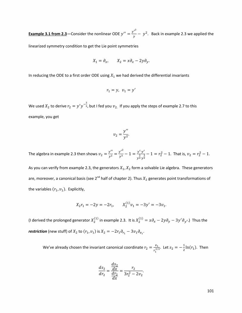
101

Example 3.1 from 2.3—Consider the nonlinear ODE

Back in example 2.3 we applied the

linearized symmetry condition to get the Lie point symmetries

In reducing the ODE to a first order ODE using we had derived the differential invariants

We used to derive

but I fed you If you apply the steps of example 2.7 to this

example, you get

The algebra in example 2.3 then shows

That is,

.

As you can verify from example 2.3, the generators form a solvable Lie algebra. These generators

are, moreover, a canonical basis (see 2nd half of chapter 2). Thus generates point transformations of

the variables ( ) Explicitly,

( )

(I derived the prolonged generator ( ) in example 2.3. It is

( ) ) Thus the

restriction (new stuff) of to ( ) is

We’ve already chosen the invariant canonical coordinate

⁄ . Let

( ). Then

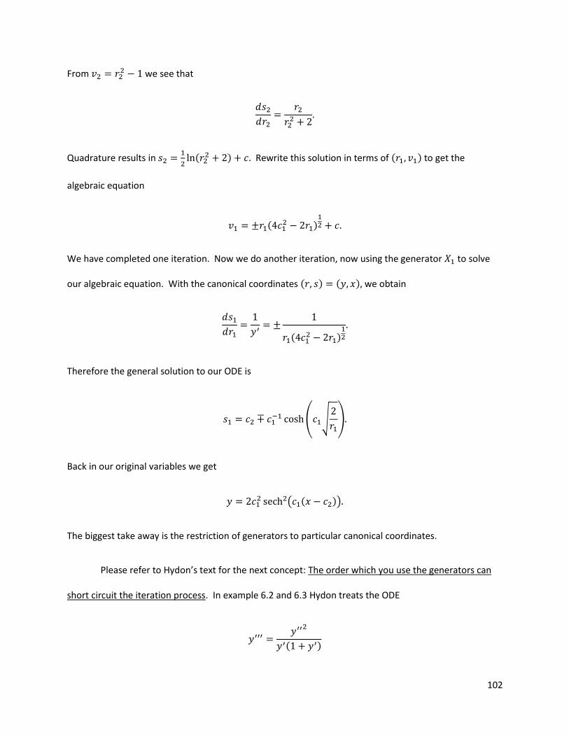
102

From we see that

Quadrature results in

(

) Rewrite this solution in terms of ( ) to get the

algebraic equation

( )

We have completed one iteration. Now we do another iteration, now using the generator to solve

our algebraic equation. With the canonical coordinates ( ) ( ) we obtain

( )

Therefore the general solution to our ODE is

( √

)

Back in our original variables we get

( ( ))

The biggest take away is the restriction of generators to particular canonical coordinates.

Please refer to Hydon’s text for the next concept: The order which you use the generators can

short circuit the iteration process. In example 6.2 and 6.3 Hydon treats the ODE

( )

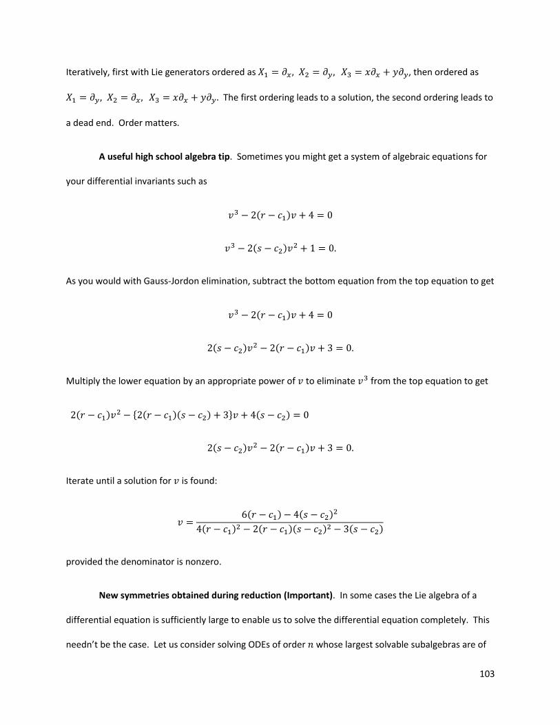
103

Iteratively, first with Lie generators ordered as , then ordered as

The first ordering leads to a solution, the second ordering leads to

a dead end. Order matters.

A useful high school algebra tip. Sometimes you might get a system of algebraic equations for

your differential invariants such as

( )

( )

As you would with Gauss-Jordon elimination, subtract the bottom equation from the top equation to get

( )

( ) ( )

Multiply the lower equation by an appropriate power of to eliminate from the top equation to get

( ) { ( )( ) } ( )

( ) ( )

Iterate until a solution for is found:

( ) ( )

( ) ( )( )

( )

provided the denominator is nonzero.

New symmetries obtained during reduction (Important). In some cases the Lie algebra of a

differential equation is sufficiently large to enable us to solve the differential equation completely. This

needn’t be the case. Let us consider solving ODEs of order whose largest solvable subalgebras are of

104

order or less. Let { } be a canonical basis for such a subalgebra. As we’ve learned in

chapter 2 in terms of the fundamental differential invariants ( ) of this subalgebra, the ODE is

equivalent to an ODE of order The general solution of the reduced ODE is an algebraic equation

( ) (1)

If we can get to this solution we are done because (1) is equivalent to an ODE of order that admits the

symmetries generated by { } If we can’t solve (1) we might have options. Each subalgebra

( ) in the solvable chain can be used to reduce the order of the ODE to an equivalent

ODE of order in the fundamental differential invariants ( ). So there is a sequence of

intermediate reduced ODEs, and it may be that one of the intermediate ODEs has NEW point

symmetries, as well as those inherited from the original ODE. With a sufficient number of new

symmetries, we might obtain the general solution of an intermediate equation in the form

( ) Then the symmetries in may be used to complete the solution of the original ODE.

Example 3.2—Consider

The linearized symmetry condition leads us to the two-

dimensional Lie algebra generated by The fundamental differential invariants are

( )

( )

Choosing the second pair of canonical coordinates and cranking the tools we’ve learned (and no new

stuff), we would find out that our ODE is equivalent to

( ) It’s symmetries are not

obvious. However, in terms of the first pair of canonical coordinates, our ODE is also equivalent to the

2nd order ODE

(

)

(

) which has an eight-dimensional Lie algebra (this is the

BIG point). The symmetries generated from are inherited form the original ODE, but the remaining

105

(larger set) of symmetries are new. These new symmetries (see Hydon example 6.5) lead us to the

solution of our ODE. (These notes give you all the step-by-step tools to work out this problem for

yourselves.)

Section 6.3 of Hydon is dedicated to a potentially deep example—the integration of third-order

ODEs with the Lie algebra ( ) Hydon present nothing new in this example, but it is interesting

because shows that the reduced ODE is our famous Riccati equation which can be transformed into the

Schrödinger equation. Is there something deep to this connection between Riccati and Schrödinger?

Hydon’s chapter seven is lengthy, connecting two of our ideas into a new toolset for ODEs, the

Lie generators we compute for an ODE via the linearized symmetry condition to the method of

characteristics to find first integrals. It’s useful for ODEs whose Lie algebra is not solvable. The method

covered in Hydon section 7.1 is limited by the need for at least generators. Section 7.2 introduces

contact symmetries and dynamical symmetries. They are defined as follows. A diffeomorphism

( ) ( ( ) ( ( )) ( ))

is a contact transformation if

( )

You can supplement material on contact transformations by looking them up in Herbert Goldstein’s

graduate text on classical mechanics. Any generator whose characteristic satisfies the linearized

symmetry condition generates dynamical symmetries (or internal symmetries (does this mean the

same as internal symmetries in quantum field theories?)). Finally Hydon section 7.3 relates integrating

factors (studied in regular botany-based ODEs) to the material in section 7.1 Why the rush?

106

How to obtain Lie point symmetries of PDEs. (A junior level course in PDEs is helpful.) There

are no new big ideas when extending from symmetry methods for ODEs to PDEs. We only deal with

more indices. Let’s begin with scalar PDEs with one dependent variable and two independent

variables and . We express an nth order ODE by

( )

We restrict ourselves for now for PDEs of the form

( )

where is one of the nth order derivatives of and is independent of It could be that is of

order provided is independent of or any derivatives of A point transformation is a

diffeomorphism

( ) ( ( ) ( ( )) ( ))

It maps the surface ( ) to the surface

( ( ))

( ( ))

( ( ))

Our goal, namely the symmetry condition for PDEs, is that we want

( )

when

( )

107

If this is so, then is a point symmetry of ( ) To see when this goal is attainable

we have to know under what conditions we may invert the equations for and (at least locally) to give

and in terms of and and similarly for all of the partial derivatives of and their counterparts

What binds the two coordinate systems together is the total derivative, one for each

independent variable. In our restricted case the total derivatives are

As you can see, total derivatives treat the dependent variable and its derivatives as functions of the

independent variables.

If the Jacobian

|

|

(2)

when ( ) then we may invert the equations for and (at least locally) to give and in terms

of and If the Jacobian we may rewrite

( ) (3)

Applying the chain rule to (3) leads us to

[

] [

] [

]

By Cramer’s rule, then

|

|

|

|

108

Higher order prolongations to higher order partial derivatives are obtained recursively by repeating the

above argument. If we let be any derivative of wrt and then

|

|

|

|

For example, the transformation is prolonged to second derivatives as follows:

|

|

|

|

|

|

|

|

Given all of this, the point transformation is a point symmetry of our PDE if

( )

when

( )

This symmetry is typically extremely complicated so we will linearize it just as we did for ODEs. Before

we do this linearization, it is worth working an easy example.

Example 3.3—I claim that

( ) (

( ))

is a point symmetry of Burger’s equation The Jacobian of the point transformation is

|

|

109

Thus

| ( )

( )

| ( )

|

( )

( )

| ( )

|

( )

|

Then ( ) . Indeed then our point transformation satisfies the

symmetry condition of when

We cannot in general pull point symmetries to PDEs out of our arses. As with ODEs, we need

tools to seek out one-parameter Lie groups of point symmetries. By seeking symmetries of the form

( ) ( )

( ) ( )

( ) ( )

(4)

we impose a set of constraints which we can exploit to tease out point symmetries. Just as for Lie point

transformations for ODEs (transformations on the plane), each one-parameter, local Lie group of point

transformations is obtained by exponentiating its infinitesimal generator

Equivalently, we can obtain ( ) by solving

( )

( )

( )

110

subject to the initial conditions ( ) ( )

A surface ( )is mapped to itself by the group of transformations generated by if

( ( )) (5)

when ( ) This condition may be expressed using the characteristic of the group,

From (5), the surface ( ) is invariant provided that when ( ) The equation for

is called the invariant surface condition, a central equation to some of the main techniques for finding

exact solutions to PDEs. Note: Equation (5) seems stupid. However, looking back at the introduction of

for ODEs, the equation for makes sense for PDEs by analogy to ODEs.

The prolongation of the point transformation (4) to first derivatives is

( ) ( )

( ) ( )

(6)

We need explicit formulae for and Let’s derive the formula for in full detail. To get plug in

the three equations of (4) up to first order into |

|, and into

|

| Recall:

|

| |

( ( )) ( ( ))

( ( )) ( ( ))| |

|

( )( ) ( )( )

Dropping all terms with of order or higher we get ( ) Now

111

| ( ( )) ( ( ))

( ( )) ( ( ))|

|

|

( )

So,

( )

Recall

for small . Thus

( ( ))( ( ))

( ) ( ) ( )

( )

Since to first order ( ) we see that

( )

If you repeat all of this work using the Jacobian and

|

| you will arrive at:

( )

We use recursion to prolong the transformation to higher order derivatives. Suppose that

( )

for some integers Then (just as for and ) with

112

|

|

|

|

We get

( )

( )

where

Alternatively, we can express the functions in terms of the characteristic, e.g.,

The higher order terms are obtained by induction on

where

.

The infinitesimal generator is prolonged to derivatives by adding all terms of the form up

to the desired order. For example,

( )

( ) ( )

113

For simplicity, we adopt the notation that the generator is understood to be prolonged as much as

necessary to describe the group’s action on all of the variables. To find Lie point symmetries, we need

explicit expressions for and Here are some (you know how to derive them). The first one is a

cut and paste and slight rearrangement from the detailed derivation of :

( )

( )

( ) ( )

( )

( ) ( ) ( )

( )

( ) ( )

( )

Lie point symmetries are obtained by differentiating the symmetry condition ( )

when ( ) wrt at We obtain the linearized symmetry condition

The restriction ( ) lets us eliminate from The we split the

remaining terms according to their dependence on derivatives of to obtain a linear system of

determining equations for and The vector space of all Lie point symmetry generators of a

given PDE is a Lie algebra, although it may not be finite dimensional.

114

Example 3.4—Consider The linearized symmetry condition is

when

Using to eliminate let’s write the linearized symmetry condition explicitly

( )

( ( ) ( )

)

After equating the terms that are multiplied by each power of we are left with the system of

determining equations:

(7)

(8)

(9)

(10)

(11)

(These equations are ordered with terms first, followed by the

terms and so forth. Solving (7) we

get

( )

where is an arbitrary function for the moment. Given this result, it follows that (8) has solution

( )

so (9) yields

( ) ( )

for some arbitrary functions and When we substitute our results into (10) and (11) we get

( )

( )

115

Since the functions and are independent of the above two equations can be decomposed by

equating powers of as follows:

Using each of the first three of these equations, we get

( ) ( ) ( ) ( ) ( ) ( )

where are functions of solely that are determined by substituting and into

and Equating equal powers of and solving the resulting ODEs. We get

(

)

Because there are ten arbitrary constants, the Lie algebra is ten dimensional.

Hydon’s text outlines a few more examples of this symmetry approach to PDEs in his chapter 8.

The method generalizes to PDEs with dependent variables ( ) and independent

variables ( ) Finally Hydon describes and cites the use of computer algebra tools.

116

Methods for obtaining exact solutions to PDEs. Just as with ODEs, the symmetry toolset we

have acquired for PDEs yields the generators of the PDE. For ODEs, we used these generators, then, to

extract invariant solutions. The same applies to PDEs.

In a typical first PDE course one learns to solve PDEs by various methods including: similarity

solutions, travelling waves, separation of variables, and so forth involving ansätze. Though not

advertised, many of these methods involve nothing more than looking for solutions that are invariant

under a particular group of symmetries. For example, PDEs for ( ) (like wave equations) whose

symmetries include and generally have traveling wave solutions of the form

( ) These solutions are invariant under the group generated by

because both and are invariants. In the same way PDEs with scaling symmetries admit

similarity solutions, which are constructed from the invariants of the group.

Let us generalize the idea to any Lie group of symmetries of a given PDE For now we

restrict ourselves to scalar PDEs with two independent variables. Recall that a solution ( ) is

invariant under the group generated by

iff the characteristic vanishes on the solution. That is, every invariant solution satisfies the

invariant surface condition

(12)

(Review the parallel theory and examples for ODEs.) Usually (12) is very much easier

to solve than the original PDE, as we have seen for ODEs. Don’t forget that we have to check

117

the solutions we get by plugging them back into the original PDE. For example, the group

generated by has the characteristic

The travelling wave ansatz ( )is the general solution of the invariant surface condition

Suppose for now that and are not both zero. Then the invariant surface condition is a first-

order quasilinear PDE that can be solved by the method of characteristics. The characteristic equations

are

If ( ) and ( ) are two functionally independent first integrals of the characteristic equation,

every invariant of the group is a function of and Often it is convenient to let one invariant play the

role of a dependent variable. Suppose WLOG that Then the general solution of the invariant

surface condition is ( ) The solution is now substituted into the PDE to determine the

function

If both and both depend on it is necessary to find out whether the PDE has any solutions

of the form These are the only solutions of the invariant surface condition that are not (locally) of

the form ( ) If is a function of the independent variables and only, then cannot yield

a solution ( ).

Example 3.5—Consider the heat equation The steps you will see below are highly reminiscent

of the kinds of PDEs you will struggle with in graduate electrodynamics (think Jackson’s text). It has

many symmetries. Consider the two-parameter Lie group of scalings generated by

118

Every generator of a one-parameter Lie group of scalings is of the form (see 2nd half of chapter 2)

for some constants and Remember that if is any nonzero constant, and generate the same

one parameter group (see chapter 2). (The group parameter is changed, but this does not affect the

group.) Therefore if we may assume that WLOG; if set

Suppose that so that

The invariant surface condition is

which is solved by integrating the characteristic equation

Carrying out the integrations yields

and

. Because in this case is independent of

every invariant solution is of the form ( ) This is equivalent to

(

) Then

( ) (

( )

( ))

( ) ( )

Therefore

(

) is a solution to the PDE if

119

The general solution of this ODE is

( ) (

) (

)

where ( ) and ( ) are parabolic cylinder functions. If is an integer, these functions can be

expressed in terms of elementary functions and their integrals. For example, if then

( ) (

)

where

( )

√ ∫

is the error function. If, on the other hand,

⁄

⁄ ∫

⁄

Substituting these results into

(

)

results in a large family of solutions which includes the fundamental solution

⁄

⁄

the error function solution

(

√ )

120

and many other well-known solutions. Get more out of Jackson’s “Classical Electrodynamics”.

Hydon’s chapter nine covers a more PDE examples, including how to get new solutions from

known solutions, and the use of nonclassical symmetries. Except for chapter seven, I’ve rendered

Hydon’s eleven chapter text more transparent to sophomore students and above. Get it. Do it.

121

Lagniappe

Once you know the simplest solution to some differential equations, you may employ very

clever algebra to extract the rest of the solutions. Enjoy the next two pages and a half. Consider a

spring-mass system with spring constant and mass It’s total energy is

where the frequency is

is the potential energy,

is the kinetic

energy, and the total energy. Let’s simplify things with

( is used in quantum mechanics instead of , ditto instead of ) Then

( )

We turn this (Hamiltonian ) H (total energy) into a Schrödinger (differential) equation by letting

√

√

Now we have (a simple quantum model of an electron oscillating from its equilibrium radius.)

( )

Let us study the commutator of and

[ ] ( ) (

√

(√ ) √

√

)

122

So [ ] As with electrons orbiting nuclei in discrete orbits with discrete energy levels, the

electrons in this model only oscillate at discrete frequencies corresponding to discrete energy levels—

the mathematics will bear this out in a page. For each integer there corresponds an energy (an

eigenvalue) and a wave function (eigenfunction) which satisfies the differential equation

Ladder algebras. For the classical equation ( ) ( )( ) For the quantum

mechanical equation this is so. We instead get

( )( ) ( ) ( )

because obviously don’t commute (thus being subject to the Heisenberg uncertainty principle).

Here is the identity operator (doesn’t do anything; it’s the one, the unit.)

Now consider

( )( ) ( )

So

( )( )

Lastly consider

( )

( )( )

( )( )( )

( )

( )( )

( ) ( )

( )

( )

( )

123

Thus

( ) (

) ( )

So the energy levels of the (harmonic oscillator) electron are equally spaced by

Let denote the lowest energy level corresponding to wave function the so-called ground

state. Then, since we can’t get to a lower energy state than the lowest energy state,

( )

Now,

( )

implies that

[( )( ) ]

but ( ) so

Therefore

must be the lowest possible energy state (the ground state). is also called

the zero point energy (energy can never be zero since

).

For shorthand, let ( ) ( ) Then (iterating times)

( ) Try plugging in. is a raising operator (or creation operator), while is a lowering (or

annihilation) operator. In quantum physics we have ladder operators for the energy of the harmonic

oscillator, angular moment, and so forth, and in particle physics (requiring relativistic quantum

124

mechanics) we have ladder operators to create or destroy particles, e.g., an electron and positron

annihilate each other to create a photon. Cool stuff.

If we can find we can find purely by our ladder algebra. Let’s find that zeroeth

eigenfunction.

( ) (

)

The solution to this simple ODE is

(

) ( )

(

) ( )

where is an arbitrary constant and ( ) are the Hermite polynomials. Then

(

) (

) ( ) (

)

(

)

(

)

(

)

(

) (

)

(

)

(

)

(

)

Indeed . We are generating the Hermite polynomials.

You have now seen that linear algebra, modern (abstract) algebra and differential equations are

not disjointed. They are bound together by the unifying methods of symmetry methods in great part

because our nature is bound by symmetries. There is more of this unifying still to go. Along the way we

will pick up topology and algebraic topology and some differential geometry. You now have at your

fingertips powerful tools to treat linear and nonlinear ordinary and partial differential equations and you

have deep insights into classical and quantum physics and the problems of mathematical physics.

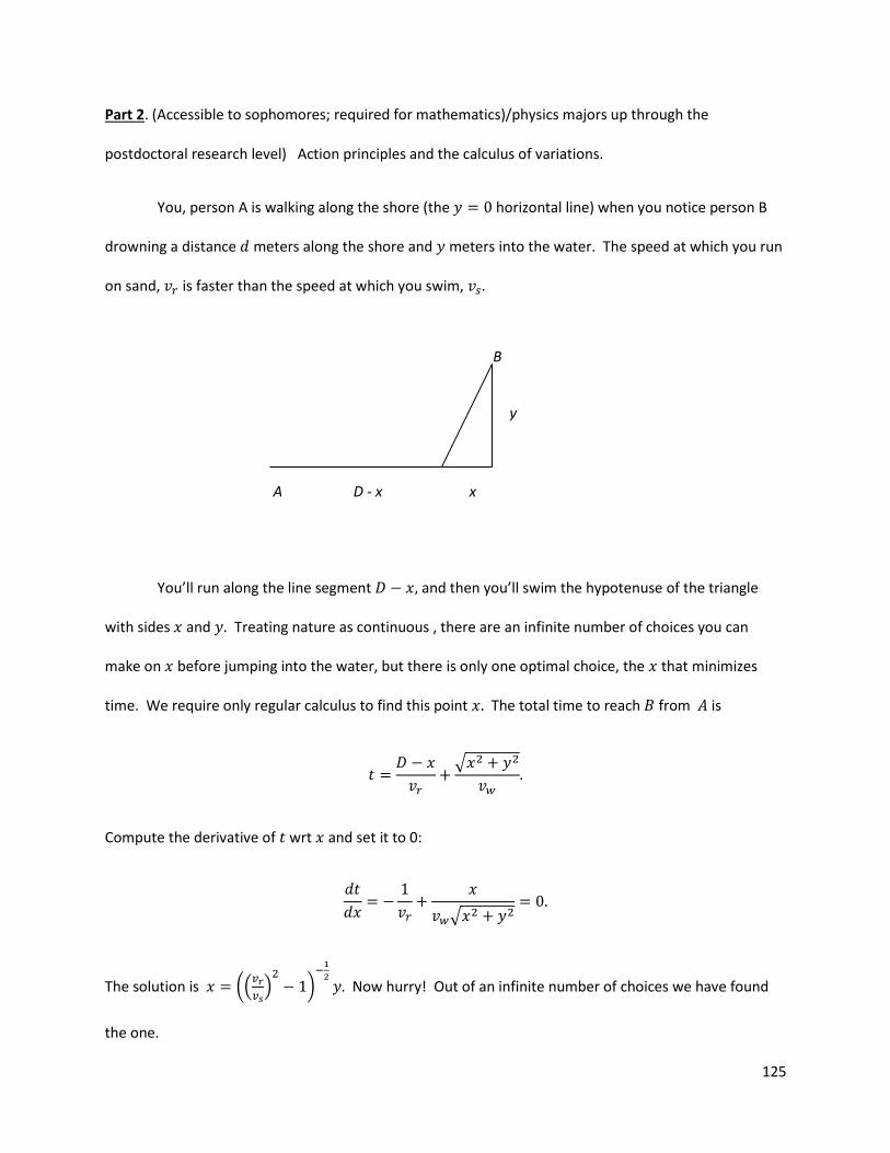
125

Part 2. (Accessible to sophomores; required for mathematics)/physics majors up through the

postdoctoral research level) Action principles and the calculus of variations.

You, person A is walking along the shore (the horizontal line) when you notice person B

drowning a distance meters along the shore and meters into the water. The speed at which you run

on sand, is faster than the speed at which you swim,

You’ll run along the line segment and then you’ll swim the hypotenuse of the triangle

with sides and Treating nature as continuous , there are an infinite number of choices you can

make on before jumping into the water, but there is only one optimal choice, the that minimizes

time. We require only regular calculus to find this point The total time to reach from is

√

Compute the derivative of wrt and set it to 0:

√

The solution is ((

) )

Now hurry! Out of an infinite number of choices we have found

the one.

B

D - x x

y

A

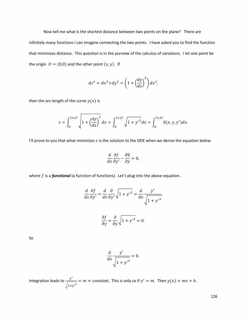
126

Now tell me what is the shortest distance between two points on the plane? There are

infinitely many functions I can imagine connecting the two points. I have asked you to find the function

that minimizes distance. This question is in the purview of the calculus of variations. I let one point be

the origin ( ) and the other point ( ). If

( (

)

)

then the arc-length of the curve ( ) is

∫ √ (

)

( )

∫ √ ( )

∫ ( ) ( )

I’ll prove to you that what minimizes is the solution to the ODE when we derive the equation below

where is a functional (a function of functions). Let’s plug into the above equation.

√

√

√

So

√

Integration leads to

√ This is only so if . Then ( ) .

127

Action principles are principles that extremize functionals, which are functions of functions,

producing either minimal or maximal functions. The fundamental laws of our universe can be expressed

in terms of action principles, as well as many emergent laws, like raindrop splashes crowning into

symmetric beads and snowflakes forming into six sided shapes. Action principles produce differential

equations that are rife with symmetries. This has happened often in particle physics, but one could

argue for the reverse case. Nature is rife with symmetries that lead us to differential equations that may

be seen as generators of solution curves which extremize some action. We shift our focus a little bit

from this “reverse” point of view if we prefer to think of symmetries as measures of invariance, a

triangle on a plane being invariant to a handful of rotations and reflections about the plane, spacetime

being invariant to continuous Lorentz transformations. This was the path to both special and general

relativity. As we have seen for differential equations, invariances can be continuous or discrete. We

have an interesting chicken-egg problem. A third point of view is that symmetries thought about in

terms of commutators and the concepts of Lie algebras is that symmetries measure interaction. (Anti-)

commutators and annihilation and creation operators of particles, be these electrons or strong nuclear

force gauge bosons, or theoretical particles such as supersymmetric particles, express interacting

particles and fields. A fourth flavor that I see is that commutators measure “entanglement” of variables,

space-time being “entangled” in special relativity by Lorentz transformations which in turn “entangle”

particles, like the electrons and positrons of the Dirac equation being forced by local relativistic

invariance to interact with (gauge boson) photon fields described in terms of vector potentials/covariant

derivatives. The mathematicians have now come to see gauge fields as essentially a measure of the

curvature of a connection on some fiber bundle, requiring a background in geometry and local and

global algebraic topology. At the end of these notes I have an essay/syllabus of good books and ideas

that render this paragraph meaningful if it isn’t yet so. These notes are themselves a skeleton of the

ideas in this paragraph. In any case, action principles are formulated using the calculus of variations.

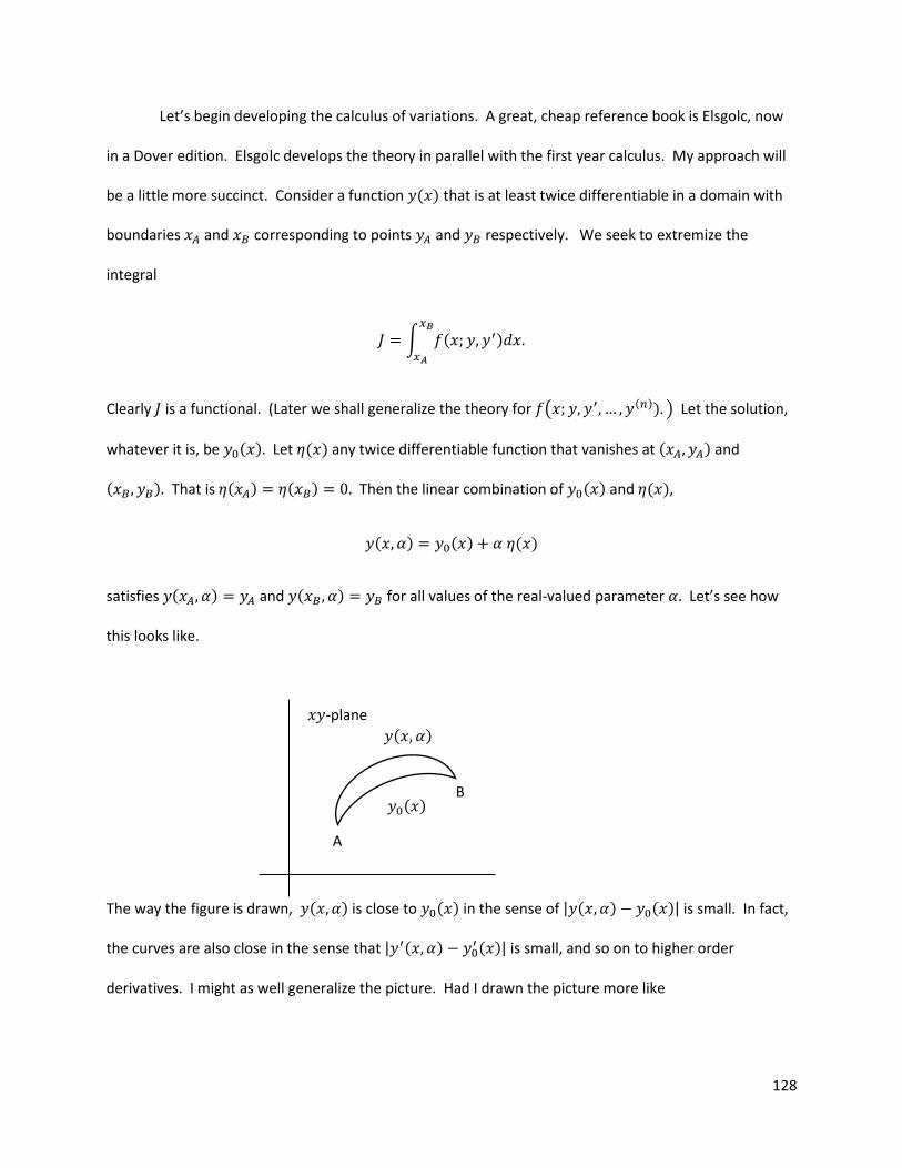
128

Let’s begin developing the calculus of variations. A great, cheap reference book is Elsgolc, now

in a Dover edition. Elsgolc develops the theory in parallel with the first year calculus. My approach will

be a little more succinct. Consider a function ( ) that is at least twice differentiable in a domain with

boundaries and corresponding to points and respectively. We seek to extremize the

integral

∫ ( )

Clearly is a functional. (Later we shall generalize the theory for ( ( )) ) Let the solution,

whatever it is, be ( ) Let ( ) any twice differentiable function that vanishes at ( ) and

( ) That is ( ) ( ) Then the linear combination of ( ) and ( ),

( ) ( ) ( )

satisfies ( ) and ( ) for all values of the real-valued parameter Let’s see how

this looks like.

The way the figure is drawn, ( ) is close to ( ) in the sense of | ( ) ( )| is small. In fact,

the curves are also close in the sense that | ( ) ( )| is small, and so on to higher order

derivatives. I might as well generalize the picture. Had I drawn the picture more like

𝑦(𝑥 𝛼)

𝑦 (𝑥) B

A

𝑥𝑦-plane

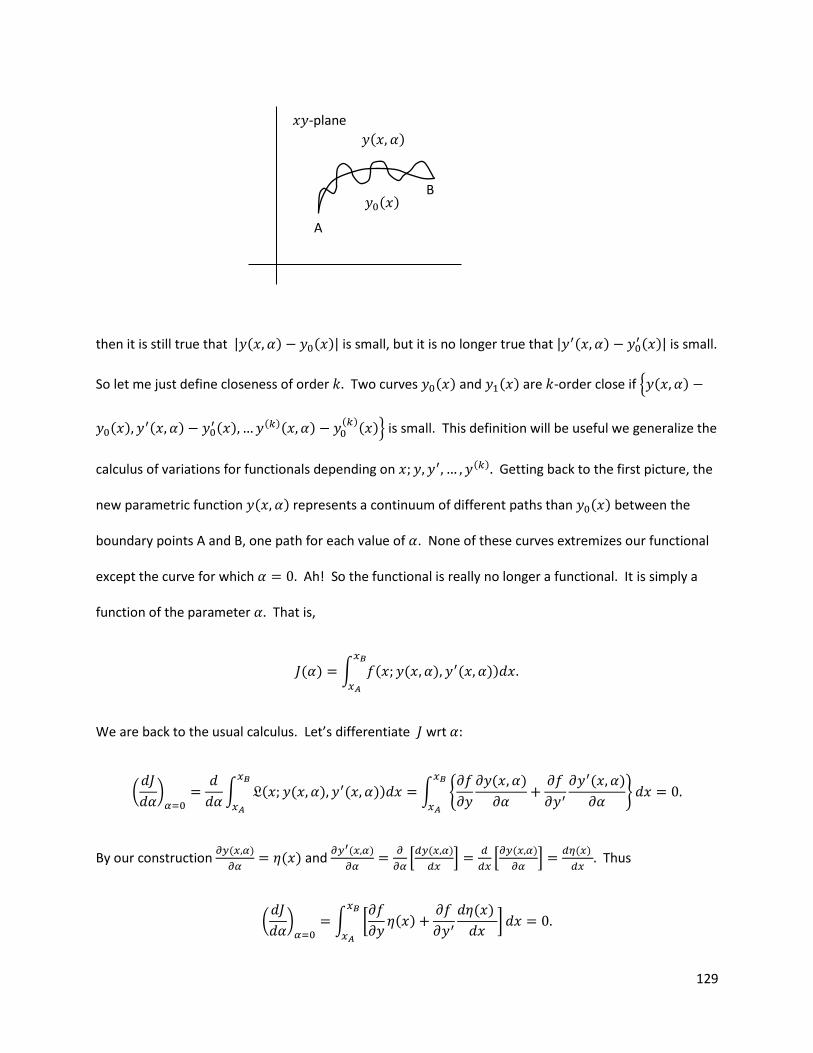
129

then it is still true that | ( ) ( )| is small, but it is no longer true that | ( ) ( )| is small.

So let me just define closeness of order Two curves ( ) and ( ) are -order close if { ( )

( ) ( )

( ) ( )( ) ( )( )} is small. This definition will be useful we generalize the

calculus of variations for functionals depending on ( ) Getting back to the first picture, the

new parametric function ( ) represents a continuum of different paths than ( ) between the

boundary points A and B, one path for each value of . None of these curves extremizes our functional

except the curve for which Ah! So the functional is really no longer a functional. It is simply a

function of the parameter That is,

( ) ∫ ( ( ) ( ))

We are back to the usual calculus. Let’s differentiate wrt

(

)

∫ ( ( ) ( )) ∫ {

( )

( )

}

By our construction ( )

( ) and

( )

[ ( )

]

[ ( )

]

( )

Thus

(

)

∫ [

( )

( )

]

𝑦(𝑥 𝛼)

𝑦 (𝑥) B

A

𝑥𝑦-plane

130

Let’s do each integral apart and evaluate the second integral using integration by parts to get

∫

( )

∫

( )

( )|

∫ ( )

(

)

The first term is zero at the boundary points. Put the remaining part above with the first term:

∫ [

(

)] ( )

This is a necessary (not sufficient) condition to have a minimum at Since ( ) is arbitrary,

(

)

Voila! We have the Euler-Lagrange differential equation. We have found a condition for finding a path

that extremizes , the Euler-Lagrange differential equation. Physicists normally write instead of

calling the Lagrangian, which is the difference of the kinetic energy and potential energy, .

In physics, action is an attribute of the dynamics of a physical system. It is a mathematical functional

which takes the trajectory, also called path or history, of the system as its argument and has a real

number as its result. Generally, the action takes different values for different paths. The Euler-Lagrange

differential equations extremize the action:

Example 1.1—Consider a spring mass system with mass and spring constant . The kinetic energy is

and the potential energy is

Thus

The Euler-Lagrange

differential equation is

There is your differential equation of motion. We’ve seen its quantum mechanical counterpart.

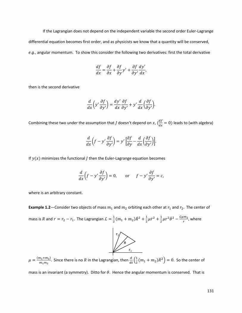
131

If the Lagrangian does not depend on the independent variable the second order Euler-Lagrange

differential equation becomes first order, and as physicists we know that a quantity will be conserved,

e.g., angular momentum. To show this consider the following two derivatives: first the total derivative

then is the second derivative

(

)

(

)

Combining these two under the assumption that doesn’t depend on (

) leads to (with algebra)

(

) [

(

)]

If ( ) minimizes the functional then the Euler-Lagrange equation becomes

(

)

where is an arbitrary constant.

Example 1.2—Consider two objects of mass and orbiting each other at and The center of

mass is and The Lagrangian

( )

where

( )

Since there is no in the Lagrangian, then

(

( )

) So the center of

mass is an invariant (a symmetry). Ditto for . Hence the angular momentum is conserved. That is

r1

B

r1

B R

132

(

) so

Here is the angular momentum of the system. This

property of conservation of some quantity was generalized by Emmy Noether (generalizing the work of

Sophus Lie). Noether's (first) theorem states that any differentiable symmetry of the action of a physical

system has a corresponding conservation law. By the way, in this example I snuck in a Lagrangian with

more than one independent variable. Can the resulting Euler-Lagrange differential equations for

multiple independent variables be coupled? Why yes they can.

Example 1.3—Using two wires of length go to your ceiling and suspend to massive bowling balls of

mass from it separated by, say, half a meter. Then couple these bowling balls by attaching a weak

spring between them. Let the spring constant be Give one ball a nudge towards the other ball, small

enough to get the ball swinging but so much as to make it run into the other ball. Eventually, thanks to

the spring between the balls, the other ball will begin to swing. Let measure the angle of the first ball

with respect to its resting position (hanging straight down), and let measure the angle of the second

ball from its resting position. Then the kinetic energy is

(

)

The potential energy is

( ) ( )

( )

If these angles are sufficiently small then

( ) ( )

( )

The last term is the source of the coupling. If you change the weak spring into a super long string, then

and the coupling is killed. So The Euler-Lagrange differential equations lead to

133

( )

( )

This folks is a coupled system of differential equations. The sum of the two equations is

( ) ( )

The difference of the top equation minus the second equation is

( ) ( ) ( )

For kicks, let ( ) and ( ) Then

Simplifying leads to

(

)

Let √

, a frequency, and let √

√

(

) √

(

) if For

solutions try

( )

( )

134

We specify initial conditions, say, ( ) . Thus For specify ( ) Then Let’s

say at the instant you nudge ball 1, it has instantaneous angular speed ( ) Then

( ) So ⁄ Note if ( ) then ( ) ( ) Then ( ) and

so ⁄ Finally,

( ) (

)

( ) (

)

The motion of one ball affects the motion of the other ball because they are coupled by a weak spring.

Example 1.4—Show and tell. The following is the Einstein-Hilbert action

∫ √

It leads to the Einstein field equations

These really are nothing more than Newton’s , but in a curved four-dimensional curved space-

time where the matter/energy fields couple to the space-time curvature (and vice-versa). The key

invariance (symmetry) that Einstein found was the indistinguishability of gravitational mass from inertial

mass. The Standard Model has its Lagrangian formalism.

If the physical system has constraints, the Euler-Lagrange differential equations need to account

for the constraints. (Imaging threading a bead onto a long wire, which we bend into a circle. Suspend

the wire circle from the ceiling and spin it. The bead might slide up and down, but always stuck to the

wire.) Without proof, if the constraints are specified by ∑ then the Euler-Lagrange

135

equations become

∑

There is a way to extend this formulism for problems involving velocity dependent potentials. Finally, if

you recall,

the theory extends to

∫ ( ( ))

The Euler-Lagrange differential equations become,

( )

( )

The calculus of variations spits out differential equations. Symmetry methods for differential equations,

though not fully general, help us unify our treatment of differential equations. Do you feel like you’re

beginning to get the keys to a large class of universes?

𝑦(𝑥 𝛼)

𝑦 (𝑥) B

A

𝑥𝑦-plane

136

Part 3. (Accessible to possibly juniors, definitely seniors; required for mathematics/physics majors up

through the postdoctoral research level) To our differential equations and abstract algebra we know

add in topology. (8.5 pages of structure to first unifying example; you’ll see the theory is nothing deep.)

Most of the topology we’ll see will be point set topology. As with abstract algebra,

mathematicians have done a fine job in rendering topology a disjointed witch’s brew of meaningless, dry

abstraction. Algebraic topology is useful you’ll see. These notes are from Gilmore’s Dover book.

The origin of point set topology is the real number line. The properties of the real number line

have been extended to higher dimensional manifolds, e.g. the -plane, the surface of the sphere, and

even abstracted to build new kinds of “weird” manifolds. Physicist pretty much stick to continuous

manifolds. Let’s review the properties of the real number line which we will use (an activity you would

do in a third or fourth year undergraduate course in real analysis). We will quickly return to Lie groups,

Lie algebras and differential equations. Our goal will be to understand Lie’s three theorems. The payoff

will be deep insight into the nature of quantum fields and general relativity.

Though not necessary, it would be good to review to at least at the level of first year calculus the

following concepts: limits, limits of functions, continuous functions, continuity, uniform continuity,

sequences, possibly limit infimum and limit supremum, Cauchy sequences, sequences of functions,

uniform convergence, and series. A very good and compact source of all of this stuff is chapter 1 (9.5

pages) of “Real Variables,” Murray R. Spiegel, Schaum’s Outline Series. The 9.5 pages of theory is

followed by nearly twenty pages of easy, step-by-step examples. Schaum’s Outline Series books are

cheap, and many of them are damned fine. Here follows the nitty gritty.

A neighborhood of a point is the set of all points such that the distance ( ) where

is any given positive number. For the real number line, the distance is defined as | | If you’re

on the place we’d have ( ) √( ) ( )

. If you’re on the surface of a sphere you’d

137

have the formula for distance on a sphere, etc. (This concept of distance, norm, or metric, is not stuck

to formulas based on the Pythagorean distance. Physicists use norms in quantum physics.)

A deleted neighborhood of a point is the set of all points whose distance from is less than ,

but excluding the point itself. On the real line this would be | |

A point is an interior point of if there exists a neighborhood of all of whose points

belong to e.g., 1 is an interior point of (0,3).

A set is open if each of its points is an interior point, e.g., (0,3).

If there exists a neighborhood of all of whose points belong to (the complement of ) then

is called an exterior point, e.g., {( ] [ )} is the complement of (0,3). Any point in the

complement of (0,3) is an exterior point.

If every neighborhood of contains at least one point of and at least one point belonging to

then is a boundary point. For (0,3) the boundary points are 0 and 3. Every neighborhood of 0

“penetrates” the interior and exterior of (0,3). Ditto 3.

The set of exterior points of is called the exterior of and the set of boundary points of is

called the boundary of

A point is an accumulation point or limit point of if every deleted deleted

neighborhood of contains points of Let {

}. Every deleted neighborhood of 0 contains

points of so 0 is a limit point of the only limit point in fact.

A set is closed if it contains all of its limit points, e.g., [0,3] is a closed. The limit points are 0 ,3.

Now we can get to two big theorems we will use.

138

Theorem 1. The union of any number (possibly infinite) of open sets is open and the

intersection of a finite number of open sets is open.

Theorem 2. The union of a finite number of closed sets is closed and the intersection of any

number of closed sets is closed.

The proofs of these theorems are easy to find; it’s well worth your time. The take away is what

these theorems forbid. For the first theorem, you can’t have an intersection of an infinite number of

open sets result in an open set. For the second theorem, you can’t have an intersection of an infinite

number of closed sets resulting in a closed set. We have a few more definitions left.

The set consisting of together with its limit points is the closure of , denoted .

A set of open sets (open intervals) is an open covering of a set if every point of belongs to

some member of If is an open covering of then is an open subcovering of

(Big one here.) A set is compact if every open covering of has a finite subcovering. For the

real line this is equivalent to being closed and bounded, e.g., [0,3]. Ditto for Getting ahead of

ourselves, the continuous group of rotations of the circle is compact on the interval

[ ], but the group of translations is noncompact.

We now need to define a topological space and a differentiable manifold, before finally starting

to connect to the continuous Lie groups we learned about in Part I. This crap will be pinned down with

concrete, accessible examples.

If is a nonempty set, a class of subset of is a topology of iff satisfies the following

three axioms:

Axiom 1: and belong to

139

Axiom 2: The union of any number (possibly infinite) of set of belongs to

Axiom 3: The intersection of any two sets of belongs to

The members of are then called -open sets (or simply open sets), and ( ) is a topological

space. Can you see how this definition of a topology has been ripped off from the real number line?

Yes. The real number line is a topology. But so are weird things like { } with

{ { } { } { } { }} satisfies all of the three axioms, hence is a topology on

Now consider { { } { } { } { }} is not a topology on because { }

{ } { { } { } { } { }} is not a topology on because { }

{ }

In this terminology then, an open set containing is called a neighborhood of . Symbolically

we write

A Hausdorff space, separated space or T2 space is a topological space in which distinct points

have disjoint neighborhood’s. This is a concept of separation. The real line is a Hausdorff space. Any

Euclidean space is a Hausdorff space. For any two distinct point on the real line I can always find tiny

enough neighborhoods for each point such that these tiny neighborhoods don’t touch each other, e.g., if

my two points are 0.000001 and 0.0000011, I can “wrap” 0.000001 in the neighborhood

(0.00009,0.00000105) and I can “wrap” 0.0000011 into the neighborhood (0.00000107,42), which are a

pair of disjointed neighborhoods.

(Updated, alternative definition of compact space): A space is compact if every infinite

sequence of points contains a subsequence of points that converges to a point in (This

involves the Axiom of Choice; mathematics is screwed because of the Axiom of Choice (see

“Mathematics, the loss of certainty,” by M. Kline.))

140

A differentiable manifold is 1. Hausdorff ( ) and 2. A collection of mappings (our Lie

symmetry transformations) (such that)

is a 1-1 mapping of an open set ( ) into an open set in

If ( ) is an open set in and ( ) is an open set in

( ) ( )

(Maximality)

and

The big idea here is to be able to work with the neighborhoods of some potentially ugly or weird

space (say the surface of a torus, the surface of a Mobius strip or Klein bottle, ( ) of our example

with the sets being letters, etc.) and map it smoothly onto small neighborhoods in Euclidean space

which is much easier to work with. In our case the spaces which we will be mapping to are the

spaces made up from -dimensional continuous Lie groups, e.g., the symmetry group ( ) (for some

ODE or PDE) being mapped (locally) to Don’t forget this mental picture. To remind ourselves of the

tie to differential equations, let me cut and paste from the Hydon text the following definition of a

continuous local Lie group.

Suppose that an object occupying a subset of , say a solution to an th order ODE, has an

infinite set of symmetries ( ), where is a real-valued parameter,

and that the following conditions are satisfied:

(L1) is the trivial symmetry, so that when (Identity)

(L2) is a symmetry in some neighborhood of zero (a point arbitrarily near zero).

141

(L3) ) sufficiently close to zero. (Closure) (Here the binary operation means

adding the parameters .) (We usually think of these parameters being small, near zero.)

(L4) Each may be represented by a Taylor series in (in some neighborhood of ), and therefore

( ) ( ) ( )

Then the set of symmetries is a one-parameter, continuous local Lie group. The term “local” refers to

the fact that the conditions need only apply in a neighborhood of The term group is used

because satisfies the definition of a group.

In slightly more jazzed up language, an -parameter topological group (or continuous group)

consists of 1-An underlying -dimensional manifold 2-An operation mapping each pair of points

( ) in the manifold into another point in the manifold. 3-In terms of a coordinate system around

we write

( )

where

In this definition we are concerned about mapping a pair of elements of a continuous Lie group into a

third element of that continuous Lie group by the group operation.

Stop and think about this mental picture. We know from Part I that there are ODEs and PDEs

whose Lie symmetries (extracted by the linearized symmetry condition) happen to be the continuous Lie

group ( ):

( )

( ) The

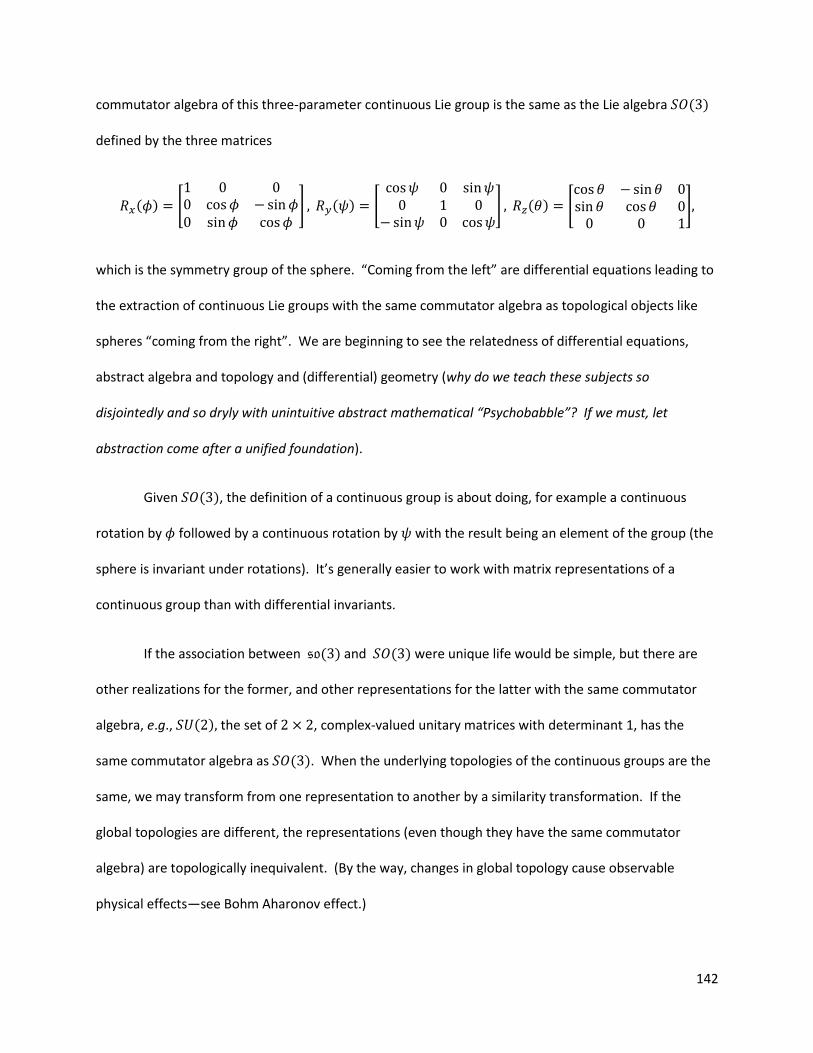
142

commutator algebra of this three-parameter continuous Lie group is the same as the Lie algebra ( )

defined by the three matrices

( ) [

] ( ) [

] ( ) [

]

which is the symmetry group of the sphere. “Coming from the left” are differential equations leading to

the extraction of continuous Lie groups with the same commutator algebra as topological objects like

spheres “coming from the right”. We are beginning to see the relatedness of differential equations,

abstract algebra and topology and (differential) geometry (why do we teach these subjects so

disjointedly and so dryly with unintuitive abstract mathematical “Psychobabble”? If we must, let

abstraction come after a unified foundation).

Given ( ), the definition of a continuous group is about doing, for example a continuous

rotation by followed by a continuous rotation by with the result being an element of the group (the

sphere is invariant under rotations). It’s generally easier to work with matrix representations of a

continuous group than with differential invariants.

If the association between ( ) and ( ) were unique life would be simple, but there are

other realizations for the former, and other representations for the latter with the same commutator

algebra, e.g., ( ) the set of , complex-valued unitary matrices with determinant 1, has the

same commutator algebra as ( ). When the underlying topologies of the continuous groups are the

same, we may transform from one representation to another by a similarity transformation. If the

global topologies are different, the representations (even though they have the same commutator

algebra) are topologically inequivalent. (By the way, changes in global topology cause observable

physical effects—see Bohm Aharonov effect.)

143

Let me give you a flavor of the difference between local and global topology. A topological

object with ( ) symmetry is as different as the sphere with ( ) as the surface of the sphere is

different than the plane generated by translations , , an issue of global topology. Walk straight

along the equator of a sphere and you will return to your initial starting position. Clearly this does not

happen if you’re on an infinite two-dimensional plane. Up to point set topology, LOCALLY a small patch

of the surface of a two-dimensional sphere looks like a little patch of the plane, an issue of. The

mathematics of Sophus Lie is local in this sense. The trigonometric functions are linearized in Taylor

series: and when A little more structure and we’ll get to an example that will

feel like an example from Part I.

In a topological (continuous) group, we have:

( ) ( )

( ( )) ( ( )) ( )

( ) ( ) ( )

( ) ( ) ( )

Part I taught us about continuous groups of Lie transformations. Continuous groups of Lie

transformations are special cases of continuous groups of transformations. A continuous group of

transformations is (a) An underlying topological space which is an -dimensional manifold together

with a binary mapping (b) A geometric space which is an -dimensional manifold,

and a mapping which obey postulate (a’): namely that obey the postulates of a

topological group, and postulate (b’): The function ( ) is continuous with the

following additional properties:

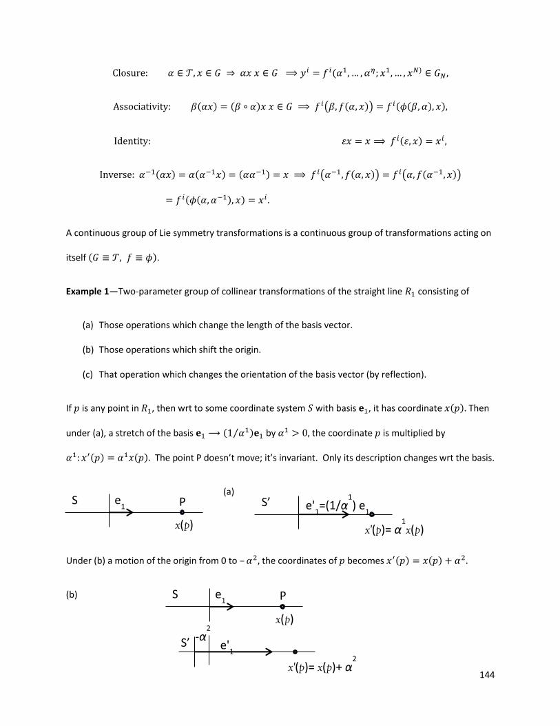
144

( )

( ) ( ) ( ( )) ( ( ) )

( )

( ) ( ) ( ) ( ( )) ( ( ))

( ( ) )

A continuous group of Lie symmetry transformations is a continuous group of transformations acting on

itself ( ).

Example 1—Two-parameter group of collinear transformations of the straight line consisting of

(a) Those operations which change the length of the basis vector.

(b) Those operations which shift the origin.

(c) That operation which changes the orientation of the basis vector (by reflection).

If is any point in , then wrt to some coordinate system with basis , it has coordinate ( ) Then

under (a), a stretch of the basis ( ⁄ ) by the coordinate is multiplied by

( ) ( ) The point P doesn’t move; it’s invariant. Only its description changes wrt the basis.

(a)

Under (b) a motion of the origin from 0 to – the coordinates of becomes ( ) ( )

(b)

e1

x(p)

S P e'1=(1/α

1) e

1

x'(p)= α1x(p)

S’

e1

x(p)

S P

e'1

x'(p)= x(p)+ α2

S’ -α2

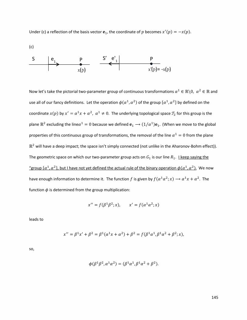
145

Under (c) a reflection of the basis vector the coordinate of becomes ( ) ( )

(c)

Now let’s take the pictorial two-parameter group of continuous transformations and

use all of our fancy definitions. Let the operation ( ) of the group { } by defined on the

coordinate ( ) by The underlying topological space for this group is the

plane excluding the line because we defined ( ⁄ ) (When we move to the global

properties of this continuous group of transformations, the removal of the line from the plane

will have a deep impact; the space isn’t simply connected (not unlike in the Aharonov-Bohm effect)).

The geometric space on which our two-parameter group acts on is our line . I keep saying the

“group { }, but I have not yet defined the actual rule of the binary operation ( ) We now

have enough information to determine it. The function is given by ( ) The

function is determined from the group multiplication:

( ) ( )

leads to

( ) ( )

so,

( ) ( )

e1

x(p)

S P e'1

x'(p)= -x(p)

S’ P

146

Now let’s check all of the conditions of our fancy definitions for a continuous group. For our example,

is a manifold since each half-plane (the half-plane to the left of and the half-plane to the right)

can be mapped 1-1 onto a part of From ( ) ( ) we identify the

coordinates of

( )

Both and are continuous. Let’s check:

Closure: ( ) and . We did this last check because,

recall, excludes the line with first coordinate zero.

Associativity: ( ( )) ( ) ( )

( ) ( ( ) )

Inverse: (

) ( ) (

).

We have to similarly check the postulates for a continuous group of transformations. Clearly

(our line) is a manifold and ( ) is continuous in all of its arguments, and

obeys

Closure: ( )

Associativity: ( ( ) ) ( ) (

) ( ( ))

Identity: ( )

147

Inverse: (

)

We may rewrite all of this structure into matrix representation form with the 1-1 mapping of

into 2 nonsingular matrices

( ) (

)

Then

(

) (

)(

) (

)

(

) (

) (

) (

)

We’ll see that matrices will have their advantages. Back in the algebraic form,

What happens if we do this twice (square it that is): ( ) ( ) ( ) ( )

In general,

( ) ( ) ∑( )

( ) ( )

If is a positive integer, the homogeneous polynomials ( ) can be used as basis

for an ( ) ( ) matrix representations of this projective group. These matrix representations

are all faithful (1-1). If N were real, the representations are dimensional, e.g., here is a faithful

representation (please refer to Gilmore’s Dover text chapter 3).

( ) (

( ) ( ) ( ) ( )

( ) ( )

)

148

Quick linear algebra review—This two page review goes well with our picture example. (Think

first year physics and/or calculus III.) A linear algebra is a collection of vectors , and a

collection , a field together with ( ) vector addition, +, ( ) scalar multiplication, ( ) vector

multiplication postulates

[A] (closure under vector addition)

( ) ( ) (associativity)

(additive identity, )

( ) ( ) (additive inverse)

[B] (closure under scalar multiplication)

( ) ( ) (associativity of scalar multiplication)

(scalar multiplicative identity)

( ) ; { } (bilinearity)

STOP HERE and we have the definition of a linear vector space, but let’s keep going to [C].

[C]

( ) ; ( ) (bilinearity)

STOP HERE and we have a linear algebra.

We can add additional postulates “[D]” but this will lead to different types of algebras. We can

add the postulate that or the postulate that Clearly these are

mutually inconsistent choices. But what would motivate adding one of the above choices over another?

149

In vector calculus, if we let we know the vector cross product: , hence we

might chose and be done with it, BUT there are other types of important linear

algebras. The set of real-valued, matrices is a linear algebra under matrix addition and scalar

multiplication by real numbers; that is, it satisfies postulates [A], [B] and [C]. If we adjoin the usual

definition of matrix multiplication by letting be defined by ( ) ∑ the space

becomes an associative algebra, the identity element being ( ) We’re about to run into

problems. If we restrict ourselves to the set of real symmetric matrices obeying ( ) =

where the stands for matrix transpose, then we can’t use normal matrix multiplication because

the product of two symmetric matrices is not generally symmetric. That is, if matrices are

real symmetric matrices, then generally ( ) ∑ real symmetric matrix. If we define

by anticommutation, { } we get a linear algebra, and . So for

these objects we have to choose postulate . For objects that are real

antisymmetric matrices , the operation must be defined by [ ]

[ ], our old friend the commutator. If we add [ ] [ ] [ ] we have a

(matrix) Lie algebra! It obeys the (matrix) Jacobi identity [ [ ]] [ [ ]] [ [ ]] So

the nature of the object determines our choices for the additional postulates [D].

In example 1.4 we looked at a change of basis. In general terms we have a vector ∑ in

coordinate system Changing coordinate systems to we have

∑

We may drop the summation symbol, the addition being implicit. Notice the matrix is on the left of

the basis vectors. We say basis vectors transform in an covariant way. On the other hand

( )

150

where I only added the parenthesis for visual effect. We see that the matrix is to the right of the

vector components Thus we say that vectors transform in a contravariant way. Summing up

We have, effectively, two bases, a “dual basis” in linear algebra, and it helps us define the dot product.

Basis vectors with low indices, transform covariantly, while basis vectors transform

contravariantly. This structure is essential for special and general relativity:

( )(

)(

)

where the matrix is the metric of special relativity (the Minkowski metric). We bury this structure

of the dot product in ordinary, 1st year calculus based physics because the metric tensor is the identity

matrix.

There are five more definitions to go in this chapter, but they will have context thanks to our

example 1. (Gilmore’s Dover text gets into how to discover most of the global properties of a

continuous group from its properties near the origin).

A local continuous group is a manifold together with a binary operation which is defined

on certain points (in particular, in a neighborhood of the identity) with the properties

1- ( ) when ( ) is defined, and is continuous where defined.

2- is continuous when defined.

3-When ( ) and ( ) are defined, [ ( ) ] [ ( )] if defined.

4-There is an identity element ( ) ( )

151

5-If is defined, then ( ) ( )

These are the properties of a neighborhood of the identity of a continuous group. Warning: Since

multiplication and inversion may correspond to points outside the neighborhood of then

multiplication and inversion are not defined in such a neighborhood. It is not always true that a local

continuous group can be embedded in a global topological group.

Two local continuous groups ( ) and ( ) are locally isomorphic if (1) there is a 1-1

mapping , (2) If and If , then and are defined iff are

defined. In addition, the manifold isomorphism must preserve the group operation ( )

As I pointed out in a previous discussion, local continuous groups and local Lie groups arise

when we linearized the group structure, e.g., the trigonometric terms in the rotation group ( ) being

linearized, We are investigating the properties of the group only near its identity.

We will have occasional use for local compactness. A space is locally compact if, around and

point a neighborhood can be found whose closure (the neighborhood with its boundary, all its limit

points) lies within the set. Our example is locally compact.

Lie groups. Let be the identity and let be some other point in the connected

component of a continuous group (the part of the group where any two points can be joined by a line).

Then and can be joined by a line lying entirely within the connected component. Choose points

on the line with the following properties:

1- lie within a common neighborhood.

152

2- lies inside some neighborhood of the identity of the identity for each value of This

can always be done with a countable number of group operations Then the group operation can be

written

( ) (

)( )

Plainly, is a product of group operations near the identity. We are interested in studying the function

( ) (

)

with small think Taylor series expansion. Then we must demand that be differentiable.

A Lie group is the connected component of a continuous group in which the composition

function is analytic on its domain of definition. (Hilbert’s fifth problem showed that the requirement

of analyticity is unnecessarily stringent.) Lie groups of transformations and local Lie groups are similarly

defined.

We are now going to start moving fast towards tying Lie’s three theorems with the symmetry

methods for differential equations we learned about in Part I. The divorce between differential

equations and algebraic topology (of which we’ve only done local algebraic topology) could happen

because Lie groups and Lie algebras have a mathematics of their own. Lie’s three theorems provide a

mechanism for constructing the Lie algebra of any Lie group, instead of us sloppily manhandling all of

the possible commutators of all of the symmetry generators. The theorems also characterize the

properties of a Lie algebra. More than that, I will show you that this mathematics underlies our general

relativity (and other theories of gravity) and quantum fields (the ones we know of and the ones we

invent). We will be working with and developing a practical example very quickly this time.

153

Let ( ) be any function defined on all points Once we choose a coordinate system in ,

we can assign each point an -tuple of coordinates:

( ) ( ) ( ) ( )

The function ( ) can then be written in terms of the parameters ( ) in coordinate system S:

( ) [ ( ) ( ) ( )]

In some other coordinate system the coordinates of will change. Therefore the structural form of

the function must change to preserve the fixed value at point

( ) [ ( ) ( ) ( )]

How do we determine if we know ? The two coordinate systems and in are related by an

element of the Lie group of transformations

( ) [ ( )]

We already know in terms of ( ). To know in terms of ( ) we must solve ( ) in terms of

( )

( ) [ ( )]

Then the complete solution to our problem is

[ ( ) ( ) ( )]

[ ( ( )) ( ( )) ( ( ))]

(1)

This solution is not very useful. Great simplification happens if we stay near the identity. For a Lie group

operation near the identity 0, the inverse given by ( ) We can then write the

coordinates ( ) as follows

154

( ) [( ) ( )] [ ( )] [ ( )] [ ( )]

|

( )

( ) [ ( )]

|

When this solution for ( ) in terms of ( ) is used in (1) we get

[ ( )] [ ( )

[ ( )]

|

]

[ ( )] [ ( )]

|

[ ( )]

To lowest order the change in the structural form of is

[ ( )] [ ( )] {

[ ( )]

|

} [ ( )]

[ ( )]

where

( )

[ ]

|

are the infinitesimal (Lie) generators of infinitesimal displacements of coordinate systems by or

simply generators. Finite displacements are obtained by repeated applications of the generators.

Whoa! In Part I we applied the (prolonged) linearized symmetry condition to differential

equations leading to (tangent vector) Lie symmetries from which we then constructed the notion of Lie

generators, but even in Part I we noticed the tendency of divorce between differential equations and Lie

groups and Lie algebras. We found an ODE and a PDE with symmetry group ( ) The present

approach to Lie generators (which I learned first) seems more fundamental: change coordinates,

linearize, get Lie generators/tangent vectors versus get arbitrary differential equations, apply linearized

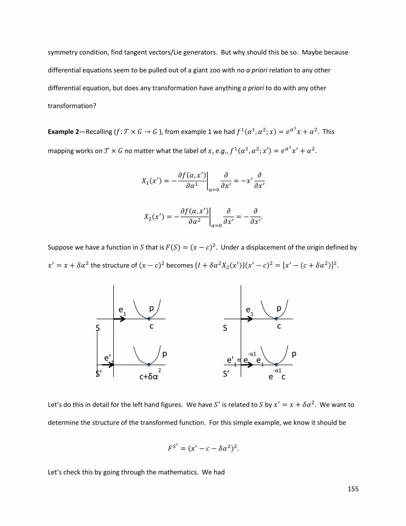
155

symmetry condition, find tangent vectors/Lie generators. But why should this be so. Maybe because

differential equations seem to be pulled out of a giant zoo with no a priori relation to any other

differential equation, but does any transformation have anything a priori to do with any other

transformation?

Example 2—Recalling ( ), from example 1 we had ( ) This

mapping works on no matter what the label of , e.g., ( )

( )

( )

|

( )

( )

|

Suppose we have a function in that is ( ) ( ) Under a displacement of the origin defined by

the structure of ( ) becomes { ( )}( ) [ ( )]

Let’s do this in detail for the left hand figures. We have is related to by We want to

determine the structure of the transformed function. For this simple example, we know it should be

( )

Let’s check this by going through the mathematics. We had

S

p

c

e1

S’

p

c+δα2

e'1

S

p

c

e1

S’

p

e-α1

c

e'1= e

-α1e1

156

[ ( )] { {

[ ( )]

|

} [ ( )]} { }

[ ( )]

Working with the right equation (remembering that we drop powers of ( ) or higher since is

small)

( ) { ( )}( ) {

} ( ) ( ) ( )

( ) ( ) ( )

( ) ( )

( ) ( ) ( ( ))

Let’s now run this work for the right hand figures. We have

( ) { ( )}( ) {

} ( ) ( ) ( )

( ) ( )

( )

Is this a stretch? To first order, Then (

) ( )

( ) Then, going back to the penultimate result, we have

( ) { ( )}( ) ( ) ( ) (

)

.

I really can justify this “cheating”. Let me show you.

In the first case I got ( ) ( ( )) with If we’re interested in

finite displacements , we merely have to exponentiate:

157

( )

{

(

)}

( )

∑

( (

)) ( ) ( )( )

( )

(

) ( ) ( ) ( )

( ) ( ) ( )

( ) ( )

( ) ( ) ( ) (( ) )

( ( ))

Now for the second case, ( ) ( )

Let’s get the finite displacement.

( )

{

(

)}

( )

∑

( (

)) ( ) ( )( )

( )

( )

(

( )

)( )

( )

( ( ) ) ( ) ( ) ( )

[( ) ] [ ]

I can’t do better. This liberty with the Taylor series of the exponential function pervades Lie theory. I’m

not 100% comfortable with it. The source author wrote

( ) [ ]

158

Infinitesimal generators for a Lie group. A Lie group of transformations acts on itself. With the

identification: geometric space topological space we identify:

( ( )) ( ( ))

[ ( )] [ ( )]

It follows that the infinitesimal generators are

(

) [ ]

|

(

)

( )

|

(2)

Since a Lie group acting on itself is a nonsingular change of basis,

‖ ( ( ))

|

‖

Example 3—Recall from example 1 that we can replace our group operation with matrix multiplication

given the following mapping,

( ) (

)

Any other matrix with the same algebra works. In material that I have yet to present, I have a reason to

switch the above matrix for

( ) (

)

This matrix works better for this example. With this new matrix representation we get

159

( ) ( ) ( ) (

) (

) (

)

Then

( )

( )

(Please go back to example 1 if all of this notation is confusing; it checks. Also keep in mind where

you’re at—in the continuous Lie group of transformations. Then

(

)

(

)

So, dropping primes, ( )

( )

|

, together with the matrix above yields

(

)

(

)

( ( )

( ))

Hence,

( )

( )

These are the generators of the continuous Lie group of transformations ( ) from the left because

are on the left in

( ) ( ) ( ) (

) (

) (

)

160

How about from the right? ( are on the right of ( ).) In other words interchange the

roles of with in equation (2) resulting in:

( )

( )

|

Then,

(

)

(

)

Thus from the right (with the as functions of the vector { ),

( ( )

( )) (

)

(

)

(

)

“On the left” we have the as functions of the vector { } whereas on the right, we have

the as functions of the vector { }. Order matters! Especially in physics! Thus there is a

“relativistic” thing happening here. The group operation may be interpreted in two different ways.

Either (A) the coordinates ( ) in coordinates system are then given in which is related back to by

( ) ( ( )) OR (2), the coordinates ( ) in coordinate system are given in which is related

back to by ( ) ( ( ) ) In (A) we have the left translation by . In (B) we have the right

translation by

Back in example 2 (with ) we derived the generators in the geometric space ( ):

( )

( )

There was no left or right in

161

( )

[ ]

|

The , while the In , where the Lie group of transformations acts on itself, and we

mapped

( )

[ ]

|

(

) ( )

|

both the and belong to Hence in we have a left and right translation. Differential equations

live in manifolds Lie symmetries (topological groups) live in . Here is the marriage:

( )

[ ]

|

Here is the divorce:

( )

[ ]

|

(

) ( )

|

Ain’t it a shame.

Infinitesimal generators for matrix groups. Way back in Part I, I titillated you with

exponentiating a matrix. The generators for matrix groups are defined analogously to how we’ve

defined generators above. If ( ) is an element of matrices, we define the

infinitesimal generators by

( )

( ) ( )

The generators constructed this way are bases for linear vector spaces since ( ) is also an

infinitesimal generator:

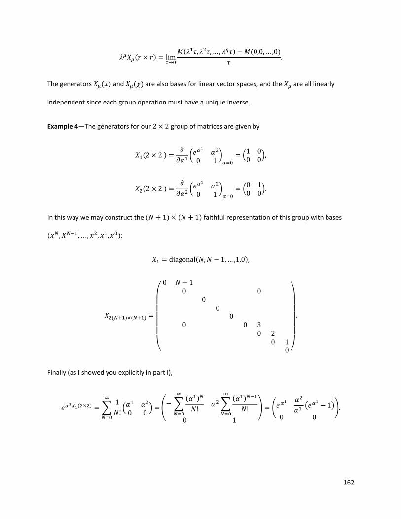
162

( )

( ) ( )

The generators ( ) and ( ) are also bases for linear vector spaces, and the are all linearly

independent since each group operation must have a unique inverse.

Example 4—The generators for our group of matrices are given by

( )

(

)

(

)

( )

(

)

(

)

In this way we may construct the ( ) ( ) faithful representation of this group with bases

( ):

( )

( ) ( )

(

)

Finally (as I showed you explicitly in part I),

( ) ∑

(

)

( ∑( )

∑( )

) (

(

)

)

163

Yet again we have another parameterization. This one is analytically isomorphic to (

) because

there is an analytic mapping between them (no proof; see Baker-Campbell-Hausdorff formulas). This

leads to another study of Lie groups: how can we classify different Lie groups if even the same group

may have more than one analytic structures describing the group multiplication? (Both and must

have the same local properties. Check them off from the definition and you show equivalence or

inequivalence.)

Commutation relations. In this section we peer into the deep underpinnings of general relativity

and quantum fields. Recall the commutator: [ ] [ ] my old friend, the end.

Recalling example 2, observe that

[ ( ) ( )] [

]

( )

and “from the left” from example 3,

[ ( ) ( )] [

]

( )

and from our matrix group,

[ ( ) ( )] ( )

ALL realizations AND representations have isomorphic commutator relations. There must be a

fundamental property of Lie algebras. What is the significance of the commutation relations? I’ve

shown lots of physics cases. Here is the mathematics. If and are elements in a commutative

(abelian) groups, then

164

If the group is not abelian, measures the amount by which differs from

where is a group element because

( )

The LHS is called the commutator of elements in a group. WOW!!! In mathematics,

noncommutativity forces us into the commutator (and the Bianchi identity) and so on). In physics, it

distinguishes between classical and quantum physics. The commutator measures the degree of physical

“entanglement”; the act of observing one of a pair of noncommuting observables leads to uncertainty in

this other observable, e.g., position, momentum and energy, time.

Now enters Sophus Lie. If and are near the identity we can expand them in terms of

infinitesimal generators (both physics and mathematics):

Now forming the product (keeping things only to first order in and ,

( )( ) (

) (

)((

)(

))

Recall that in linearized regime ( )( )

…. After lots of algebra which you

know by now how to do,

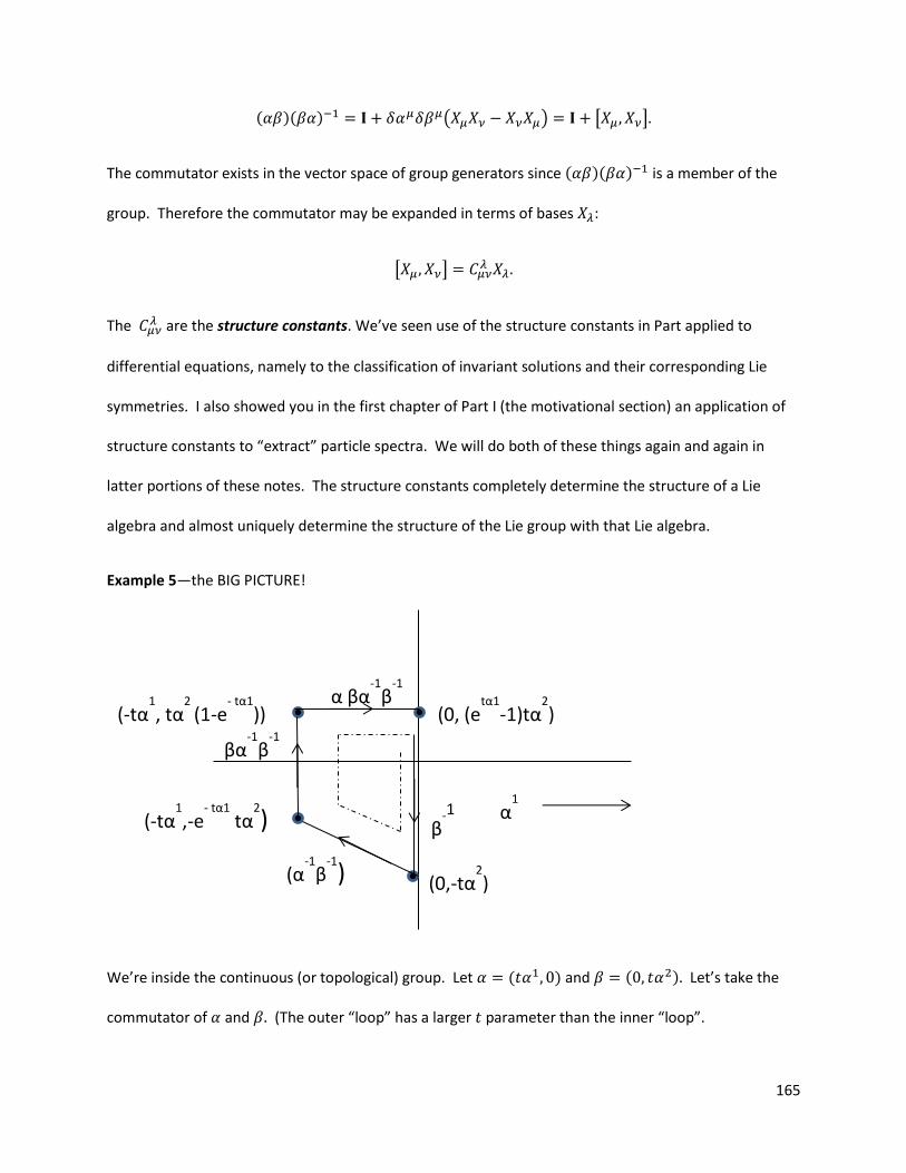
165

( )( ) ( ) [ ]

The commutator exists in the vector space of group generators since ( )( ) is a member of the

group. Therefore the commutator may be expanded in terms of bases :

[ ]

The are the structure constants. We’ve seen use of the structure constants in Part applied to

differential equations, namely to the classification of invariant solutions and their corresponding Lie

symmetries. I also showed you in the first chapter of Part I (the motivational section) an application of

structure constants to “extract” particle spectra. We will do both of these things again and again in

latter portions of these notes. The structure constants completely determine the structure of a Lie

algebra and almost uniquely determine the structure of the Lie group with that Lie algebra.

Example 5—the BIG PICTURE!

We’re inside the continuous (or topological) group. Let ( ) and ( ) Let’s take the

commutator of and (The outer “loop” has a larger parameter than the inner “loop”.

α1

(0,-tα2) (α

-1β

-1)

β-1

βα-1β

-1

α βα-1β

-1

(-tα1,-e

- tα1 tα

2)

(-tα1, tα

2 (1-e

- tα1)) (0, (e

tα1-1)tα

2)

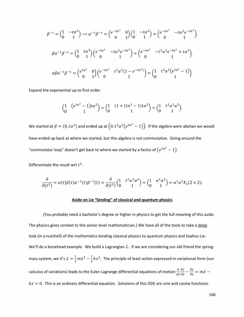
166

(

) (

) (

) (

)

(

)(

) (

)

(

) (

( )

) ( (

)

)

Expand the exponential up to first order.

( ( )

) (

( ( )

) (

)

We started at ( ) and ended up at ( ( )). If the algebra were abelian we would

have ended up back at where we started, but this algebra is not commutative. Going around the

“commutator loop” doesn’t get back to where we started by a factor of ( )

Differentiate the result wrt

( ) ( ) ( ) ( ) ( )

( )(

) (

) ( )

Aside on Lie “binding” of classical and quantum physics

(You probably need a bachelor’s degree or higher in physics to get the full meaning of this aside.

The physics gives context to the senior level mathematician.) We have all of the tools to take a deep

look (in a nutshell) of the mathematics binding classical physics to quantum physics and Sophus Lie.

We’ll do a bonehead example. We build a Lagrangian . If we are considering our old friend the spring-

mass system, we it’s

The principle of least action expressed in variational form (our

calculus of variations) leads to the Euler-Lagrange differential equations of motion

This is an ordinary differential equation. Solutions of this ODE are sine and cosine functions.

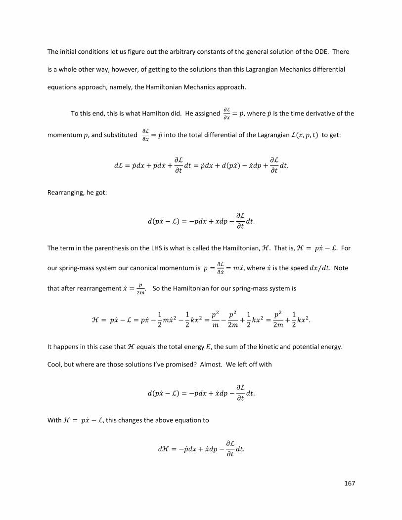
167

The initial conditions let us figure out the arbitrary constants of the general solution of the ODE. There

is a whole other way, however, of getting to the solutions than this Lagrangian Mechanics differential

equations approach, namely, the Hamiltonian Mechanics approach.

To this end, this is what Hamilton did. He assigned

, where is the time derivative of the

momentum , and substituted

into the total differential of the Lagrangian ( ) to get:

( )

Rearranging, he got:

( )

The term in the parenthesis on the LHS is what is called the Hamiltonian, That is, For

our spring-mass system our canonical momentum is

where is the speed ⁄ Note

that after rearrangement

So the Hamiltonian for our spring-mass system is

It happens in this case that equals the total energy the sum of the kinetic and potential energy.

Cool, but where are those solutions I’ve promised? Almost. We left off with

( )

With this changes the above equation to

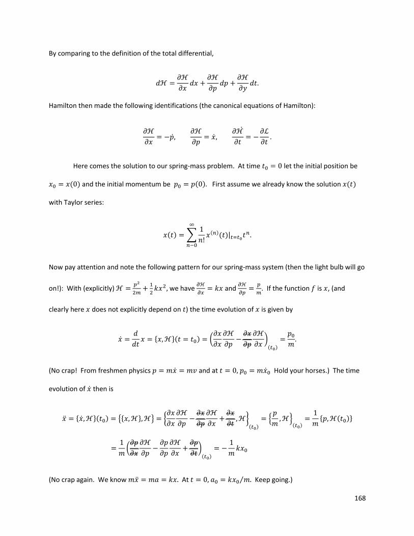
168

By comparing to the definition of the total differential,

Hamilton then made the following identifications (the canonical equations of Hamilton):

Here comes the solution to our spring-mass problem. At time let the initial position be

( ) and the initial momentum be ( ) First assume we already know the solution ( )

with Taylor series:

( ) ∑

( )( )|

Now pay attention and note the following pattern for our spring-mass system (then the light bulb will go

on!): With (explicitly)

we have

and

. If the function is , (and

clearly here does not explicitly depend on ) the time evolution of is given by

{ }( ) (

)( )

(No crap! From freshmen physics and at Hold your horses.) The time

evolution of then is

{ }( ) {{ } } {

}

( )

{

}

( )

{ ( )}

(

)( )

(No crap again. We know At ⁄ Keep going.)

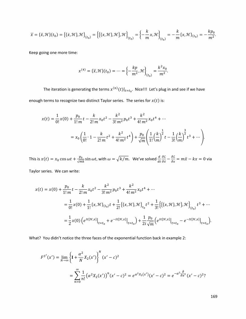
169

{ }( ) {{ } }( )

{{{ } } }( )

{

}

( )

{ }( )

Keep going one more time:

( ) { }( ) {

}

( )

The iteration is generating the terms ( )( )| Nice!!! Let’s plug in and see if we have

enough terms to recognize two distinct Taylor series. The series for ( ) is:

( )

( )

(

)

√ (

(

)

(

)

)

This is ( )

√ with √ ⁄ We’ve solved

via

Taylor series. We can write:

( ) ( )

( )

{ }( )

{{ } }

{{{ } } }

( )

( ) ( [ ]|

[ ]|

)

√ ( [ ]|

[ ]|

)

What? You didn’t notice the three faces of the exponential function back in example 2:

( )

{

(

)}

( )

∑

( (

)) ( ) (

)( )

( )

170

In general for some , what is

[ ]

(

[ ])

(

∑

({ } ) )

(∑ [ ]

( [ ])

)

([ ] ∑

( )

( [ ])

)

Let Then

∑

( )

( [ ])

∑

( [ ]) [ ]

Thus, alas,

(

[ ])

[ ]( ) [ ]|

This is the classical physics version of the Schrödinger equation.

Turning physics to mathematics, if is any function of , namely ( ) then

( )

{ }

where { } is the Poisson bracket. If is any function of and but does not explicitly depend on

time, then

and thus

{ } { } (This was the case for the spring-mass problem,

and thus the function didn’t explicitly depend on . Yet we generated ( ) via

“exponentiation” ) As we did with the physics example, let’s pretend we know ( ) Its Taylor series is

( ) ∑ ( )

( )

171

As with our physics example, now you can check that:

( ) ( )( ) { }( )

( ) ( ) { ( ) } {{ } }( )

( ) ( ) { ( ) } {{{ } } } ( )

and so on, giving us ( ) ( )∑

{ {{ } } }

( )

(

) ( ){ } The exponential notation merely represents the series. We have generated ( )

explicitly in . It follows as before that

( )

|

( ){ }|

({ } ( ){ })

Now to quantum physics and Lie’s work. One historical approach from classical physics to

quantum physics was found by assigning classical quantities to differential operators thusly,

The hats denote differential operators. The Poisson brackets become Lie commutators.

The classical Hamiltonian of our spring-mass system is

Classical physics has been transformed to the quantum physics Schrödinger equation

( ) [

(

)

] ( )

( )

( )

172

As with our classical example, we can do quantum physics via another approach other than

solving Schrödinger’s equation. To this point in the aside I’ve been fairly rigorous with the mathematics.

I now proceed merely to outline the connection between quantum physics and Lie generators. (To do

quantum mechanics you have to be up to speed on the linear algebra of unitary and hermitian matrices

and operators.) Given that the Hamiltonian is the infinitesimal (Lie) generator of time translations there

is a time evolution operator defined in quantum physics (developed by analogy to classical physics):

( )

Then in textbooks it is shown that

( ) ( ) ( )

Together these two equations lead to

( ) ( ) ( ) (

) ( )

Algebra leads to

( ) ( )

( )

In the limit of small we get Schrodinger’s equation

( ) ( )

One then goes on in quantum physics considering Hamiltonians which do or do not depend on time.

Did you note that

for our classical (and hence quantum) Hamiltonian? In the spring-

mass system the energy is a constant. It never changes. It is invariant under transformations of time

173

(the passage of time forward, or run backwards in a movie). The Hamiltonian is the infinitesimal (Lie)

generator of time translations. Abstract mathematics, meet physical context.

Historically, three different pictures, all equivalent, of quantum mechanics arose from three

different points of view. In the Schrödinger picture the state vectors (wave functions) carry time

dependence while the operators stay fixed in time, in the Heisenberg picture is the opposite. In the

interaction picture, both state vectors and operators share time dependence. We have seen how this

can happen in the study of Lie groups and algebras. Are we dealing with the algebra here

or here So some people developed quantum mechanics via Lagrangian mechanics, Hamiltonian

mechanics, Hamilton-Jacobi action angle mechanics, Poisson Brackets. Richard Feynman used the

Lagrangian in his (the fourth approach) path over histories formulation of quantum physics:

( ) ∑ ∫

Lastly, in quantum physics we see the smooth evolution of a smoothly spread wave function

pertaining to, say, an electron orbiting an atomic nucleus. The iterated (or “exponentiated” Taylor

series) approaches is more reminiscent to particle physics where particles can be created or annihilated

(recall the ladder algebra we reviewed in the lagniappe). Each term in the series iterated by a small

can be seen as particles interacting among each other: an electron being annihilated by a positron, a

photon thus being created, or the other way around, the photon splitting into an electron-positron pair.

In quantum field theories, we speak of 2nd quantization. With these notes, up to this point, you already

have good unified, symmetry-based foundations in the underlying mathematics and physics. Shall we

get back to business? End Aside.

174

Brief aside for the advanced graduate student/postdoc in particles and fields.

Recall the figure of example 5, of taking a round trip in the Lie group space in terms of the

commutator, and recall that if the group is nonabelian, the commutator measures the amount by

which differs from

By taking a round trip in this context by parallel transport, and requiring local gauge invariance, Ryder’s

text (section 3.6) shows how the covariant derivative arises such that the commutator of the covariant

derivative operators leads to gauge fields: (the are (vector) guage potentials)

[ ] [ ] { [ ]}

Then he shows how this mathematics parallels the mathematics of general relativity, the quantity being

analogous to the field tensor , the Riemann-Christoffel curvature tensor

I love step-by-step books. “Quantum Field Theory,” 2nd ed., L. H. Ryder, Cambridge, 1996 is a step-by-

step introduction to QFT. I hope that these notes enrich your understanding of quantum fields and

general relativity. Later, after I’ve covered algebraic topology dealing with global properties of

symmetry groups, I’ll have an aside on how mathematicians have generalized the concept of vector

potential/covariant derivative with differential forms and connections on principle fiber bundles.

Lie’s first theorem. (Review examples 1 -3. Keep and in mind; the Greek

letters are elements of the continuous group ( -dimensional) they are the Lie symmetries for us. The

coordinates ( ) are for the points in the continuous geometric group ( -dimensional). The

coordinates system is relative to frame S.

175

If

( ) [ ( )]

is analytic (smooth; expandable in a Laurent (or Taylor) series) then

[ ]

∑

( ) ( )

where ( ) is analytic.

Proof. If we transform from coordinate system

the coordinates of any point will

change successively from ( ) to ( ) to ( ). Suppose is an operation near the identity,

Then ( ) will be close to ( ) and the difference

( ) ( ) ( )

can be computed in two different ways:

( ) ( ) [ ]

( ) ( ) [ ]

The middle terms are differential translations in The right hand terms are group actions from

In terms of , and in terms of the linearized Taylor translations, the equation for ( )

leads to

[ ]

|

( )

Clearly we’ve identified the ( ) with the

[ ]

|

. Back in ,

176

( ) ( )

( )

|

( )

where ( ) is a nonsingular matrix identified with

( )

|

The inverse of ( ) is ( )

( ) ( ) ( )

( )

Therefore,

( )

( ) ( )

This simplifies to

( )

In terms of the displacement near induced by infinitesimal displacements at the identity, the

displacement at ( ) is given by. (The result for is substituted into the equation for )

( )

( ) ( )

Differentiating wrt to results in:

∑

( ) ( )

Since ( ) and ( ) are analytic,

( )

[ ]

|

177

( )

( )

|

are also analytic.

Example 6—(The theorem made concrete.) Sticking with examples 1-4, if ( ) is a transformation,

and ( ) is near the identity, then

( )

Since is near the , we write ( ) ( ). Recall from our previous

examples that and So

( )

( ) ( )

In matrix form,

(

) (

) (

)

Inverting and solving for we get:

(

) (

)

(

) (

)(

)

178

Then which is in (Recall: ) and the results of our solution for

which live in as do leads to

( )

Then

The formal expression

∑

( ) ( )

can also be used to determine these differential equations:

( )

( )

|

(

)

(

)

( )

[ ]

|

(

)

(

)

Thus we have

(

) (

) (

) (

)

179

Sophus Lie decomposed partial differential equations into the product of two matrices, one depending

on the transformation parameters and the other depends on the initial conditions ( ) This is a

generalization of the problem of finding solutions for systems of simultaneous linear partial differential

equations with constant coefficients

( )

which can be treated by standard algebraic (Part I) techniques.

Lie’s second theorem. The structure constants are constants. If are generators of a Lie

group, then the coefficients given by the commutators [ ]

are constants. Before

proceeding to the proof, note this critical fact: The differential equations

∑

( ) ( )

do not always have a solution. The equations

have not solutions for

Note also that the necessary and sufficient conditions for the existence of a unique solution with

initial conditions

[ ]|

is that all mixed derivatives be equal

180

These are called the integrability conditions.

Proof. We apply the integrability conditions to the equation proven in Lie’s first theorem

[ ]

∑

( ) ( )

{ ( )

( )}

{ ( )

( )}

This leads to

( )

( )

( )

( )

( )

( )

( )

( )

Rearrange this result to

( )

( )

( )

( )

( )

( )

( )

( )

Replace the terms

appearing on the left by

( )

( )

( )

( ) ( )

( )

( )

( )

( )

( ) ( )

( )

The rearranged equation becomes

( )

( ) ( )

( )

( ) ( )

( )

( )

( )

( )

( )

( )

181

Changing to on the LHS, and to on the RHS (which is okay since we didn’t lose any terms with the

new labels

( )

( ) { ( )

( )

( )

( )

} {

( )

( )

} ( )

The terms ( ) on the LHS can be moved to the RHS by multiplying both sides of the equation by the

inverses of the ( ) namely the ( ) This renders the LHS only a function of . The LHS “lives” in the

differentiable manifold On the RHS is almost only a function of The RHS is almost an animal living

in The term ( ) is a function of and cannot be moved to the LHS since it is an matrix.

We can circumnavigate this problem if we observe that these arguments hold for a Lie group of

transformations. Isomorphic arguments hold for a Lie group. That is we can make the following

identifications

( ) ( )

( )

( )

The shit happening in is happening isomorphically in (Go back to the example for Lie’s first

theorem and checkout the parallelism for yourself.) Then our almost separated example becomes

( )

( ) { ( )

( )

( )

( )

} {

( )

( )

} ( )

Let’s multiply the equation by the inverses of ( )

( ), and the inverse of ( )

( ) {

( )

( )

( )

( )

}

( ) ( ) {

( )

( )

}

Since and are arbitrary elements of we have a “classic” separation of variables situation. Both

sides must equal a constant, namely the equation We have separation of variables:

182

( )

( )

( )

( )

( )

So back in the isomorphic differentiable manifold we now have nirvana.

( )

( )

( )

( )

( )

1. For a Lie group of transformations (in the geometric manifold ) with infinitesimal generators given by

( ) ( )

|

( )

the commutator relations are

[ ( ) ( )] [ ( )

( )

] (

( )

)

( )

2. For a Lie group with generators (in )

( ) ( )

|

( )

the commutation relations are obtained in an isomorphic way:

[ ( ) ( )] [ ( )

( )

] [ ( )

( )

( )

( )

]

(

( )

)

( )

We have now shown that the structure constants are constant for a Lie group, a Lie group of

transformations, and for any of their analytic realizations or matrix representations. Quod Erat

Demonstrandum dudes.

Example 7—The PDE from example 6

183

(

) (

)(

) (

)

for x in terms of are

( )

( )

Therefore, we do not violate the integrability condition that all mixed derivatives be equal

so we can find a unique solution to these PDEs with unique initial value ( )

The structure constants can be found from the group composition function Since they are

constant, they can be evaluated at any element. At the identity element ( ) ( ) with

so that ( )

( ) (but because it is a translation away from ) our old equation

( )

( )

( )

( )

( )

Collapses to

( )

( )

( )

( )

|

For our continuing example with ( ) ( ) we readily compute

( )

( )

184

Lie’s third theorem. The structure constants obey

Proof. From

( )

( )

|

we have

( )

( )

|

The last equation is trivial, a trivial consequence of the Jacobi identity

[[ ] ] [[ ] ] [[ ] ]

The Jacobi identity follows from the associativity of the group multiplication. The Jacobi identity bears a

strong resemblance to

( ( ) ( ))

( )

( )

( ) ( )

This is why the Lie bracket [ ] is sometimes called a derivative.

Example 8—Four of the eight structure constants for our elementary Lie group are necessarily zero by

the antisymmetry requirement:

The only remaining four structure constants are independent and must be computed explicitly:

185

(Important to physicists). The structure constants for a Lie algebra provide a matrix

representation for the algebra. Generally, this representation is unfaithful. The representation is

obtained by associating with ( ) and matrix ( ) whose matrix elements are

given by ( )

Theorem. ( )

is a representation for the Lie algebra of the commutators

Proof. Let’s show that and have isomorphic commutator algebra.

([ ]) ( )

( )

( )

( )

The Jacobi identity tells us

(

)

Then [ ]

( )

Since matrix multiplication is well defined, these matrices trivially satisfy

the Jacobi identity; they also form a basis for a linear vector space. Since and have is isomorphic

commutation relations, the provide a representation of the

Example 9—From our above structure constants, we construct a matrix representation for our

two-dimensional Lie group:

(

) (

)

Have we seen these before? Physicists this representation is sometimes called the adjoint or regular

representation, and it is used extensively in the study of the properties of Lie algebras, in particular

when we seek to classify the various types of Lie algebras.

186

Converses of Lie’s three theorems. Lie’s three theorems show that for each Lie group there is a

corresponding Lie algebra. These three theorems characterize the Lie algebra by its structure constants.

The Lie algebra is uniquely determined, up to a change of basis, by the Lie group. Now we ask, given a

Lie algebra, can we find an associated Lie group? No. There is generally not a 1-1 correspondence

between Lie groups and algebras. Many Lie groups may have the same Lie algebra (recall Part I ODEs

and PDEs with the same Lie group symmetries (as analytic realizations), but among all of the groups with

the same Lie algebra there is only one that is simply connected. This simply connected group is the

universal covering group. I have yet to build up the little bit of algebraic topology required to deal with

the converses of Lie’s three theorems. The essence of the converses of Lie’s three theorems is finding

restricted cases for when one may uniquely associate a Lie algebra to a Lie group. The theorems are

stated and proved in “An Introduction to the Lie Theory of One-Parameter Groups,” Cohen, P. M., New

York: Stechert, 1931. The converses of Lie’s three theorems establish that there is a 1-1 correspondence

between simply connected Lie groups and Lie algebras, but these converse theorems do not provide a

method of constructing the analytic group multiplication ( ) from the Lie algebra. Taylor’s

theorem goes to doing this construction in a canonical way. Physicists, Taylor’s theorem lies at the

heart of why we were able to find the time evolution of physical systems via iteration (exponentiation).

It’s extension underpins time ordering operators in path integral applications to quantum physics.

Example 10—Let’s motivate the theorem with an example first. It helps. We keep with the chain of

examples we have been using since example 1. For our two-dimensional group, this is a straight line:

( ) (Recall: ( ) ( ) but we have so ( )

( ) ( is the name for the straight line; the RHS is the operational description of the line.) This

is a straight line in the Lie group. Let

( ) ( ) (

)

187

Then it follows that

( ) (

)

Now let’s repeat this for the straight line ( )

( ) ( ) (

)

Thus

( ) (

)

Lastly, consider the straight line ( ) Then ( ) (

) So

( ) (

) (

) ( )

( )

I hate shenanigans. The source author didn’t show the intermediate steps.

(

)

( ). (This has a smell of bogusness.) But now ( ) above compares well with ( )

( (

(

)

). Now let’s see about Taylor’s theorem for Lie groups.

Taylor’s theorem for Lie groups. There exists an analytic mapping ( ) in which

every straight line through the origin is a one-dimensional abelian subgroup. The Lie group operation

corresponding to the Lie algebra element is

Proof. Since ( ) ( )

(see Lie’s 2nd theorem) we may write

( ) as

( ) ( )

188

(Clever, since ( )

leaves only

( ).) When we look at the straight line ( )

through the origin of the Lie algebra, the are functions of the single parameter

( )

[ ] ( ) ( )

Note that

. Since the coordinates of the fixed point [[ ( )] are now reduced to being

functions of a single parameter we can write

( ) ( ) ( )

Then our differential equation ( )

reduces to

( ) ( ) [ ] [ ( )]

( ) ( )

Since the ( ) are arbitrary, we have the following matrix equation

( ) [ ] [ ( )]

( )

which is a first-order total differential equation for the matrix ( ) with initial conditions ( )

Thus,

( )| [ ] [ ( )]

( ) [ ( )]

(I went back to Lie’s first theorem to see that [ ] because its inverse ( ) is the identity.) The

total differential equation has solution

( ) ∑

[ [ ( )]

]

( )

( )

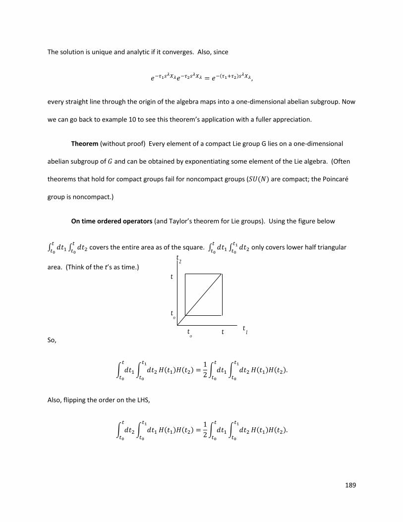
189

The solution is unique and analytic if it converges. Also, since

( )

every straight line through the origin of the algebra maps into a one-dimensional abelian subgroup. Now

we can go back to example 10 to see this theorem’s application with a fuller appreciation.

Theorem (without proof) Every element of a compact Lie group G lies on a one-dimensional

abelian subgroup of and can be obtained by exponentiating some element of the Lie algebra. (Often

theorems that hold for compact groups fail for noncompact groups ( ( ) are compact; the Poincaré

group is noncompact.)

On time ordered operators (and Taylor’s theorem for Lie groups). Using the figure below

∫

∫

covers the entire area as of the square. ∫

∫

only covers lower half triangular

area. (Think of the t’s as time.)

So,

∫

∫

( ) ( )

∫

∫

( ) ( )

Also, flipping the order on the LHS,

∫

∫

( ) ( )

∫

∫

( ) ( )

to t

1

to

t2

t

t

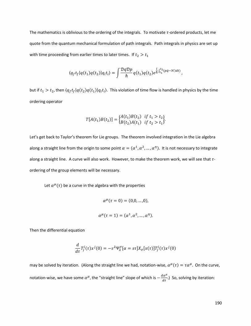
190

The mathematics is oblivious to the ordering of the integrals. To motivate -ordered products, let me

quote from the quantum mechanical formulation of path integrals. Path integrals in physics are set up

with time proceeding from earlier times to later times. If

⟨ | ( ) ( )| ⟩ ∫

( ) ( )

∫ ( ) )

but if then ⟨ | ( ) ( )| ⟩. This violation of time flow is handled in physics by the time

ordering operator

[ ( ) ( )] { ( ) ( ) ( ) ( )

}

Let’s get back to Taylor’s theorem for Lie groups. The theorem involved integration in the Lie algebra

along a straight line from the origin to some point ( ) It is not necessary to integrate

along a straight line. A curve will also work. However, to make the theorem work, we will see that -

ordering of the group elements will be necessary.

Let ( ) be a curve in the algebra with the properties

( ) ( )

( ) ( )

Then the differential equation

( ) ( ) [ ] [ ( )]

( ) ( )

may be solved by iteration. (Along the straight line we had, notation-wise, ( ) On the curve,

notation-wise, we have some the “straight line” slope of which is

) So, solving by iteration:

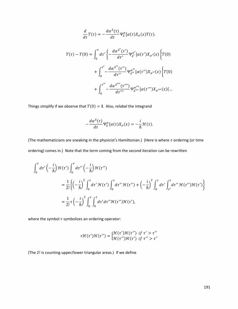
191

( )

( )

[ ( ) ( ) ( )

( ) ( ) ∫ {

( )

[ ( ) ( ) { ( )

∫

( )

[ ( ) ( ) { ( )

∫

( )

[ ( ) ( ){

Things simplify if we observe that ( ) Also, relabel the integrand

( )

[ ( ) ( )

( )

(The mathematicians are sneaking in the physicist’s Hamiltonian.) (Here is where -ordering (or time

ordering) comes in.) Note that the term coming from the second iteration can be rewritten

∫ (

)

( )∫ (

)

( )

{(

)

∫

( )∫

( ) (

)

∫ ∫

( ) ( )}

(

)

∫ ∫ ( ) ( )

where the symbol symbolizes an ordering operator:

( ) ( ) { ( ) ( )

( ) ( )

(The 2! Is counting upper/lower triangular areas.) If we define

192

( ) ∫ ( )

{

then we can write

( ) ( ) ( ) ( ) ( )[ ( ) ( )]

Clearly the -ordered product is not equal to the usual product unless the commutator vanishes. Third

and higher order iterations can be treated analogously. The iterative solution is then

( ) (

∫ ( )

)

This result collapses to the straight line solution over a straight line (see Gilmore’s Dover text.) I

personally understand every section in the notes well except for this section. The physicist’s version of

all of this for path integrals is far more sensible to me—apologies.

Topological concepts. Recall that a space is connected if any two points in the space can be

joined by a line (in the sense of “line” we used to prove Taylor’s theorem for Lie groups), and all points

of the line lie in the space.

Example 11—Still keeping with our running example, the topological space (I’ve been lazily writing )

is not connected because any line joining, say (1,0) and (-1,0) must contain a point ( ) which is

not in If you go back to example 1, you’ll recall we had ( ) ( ) Thus

( ) The axis splits

If is any point, we can look at the set of points connected to e.g., all points in the left half-

plane are connected to (-1,0); all points in the right half-plane are connected to (1,0). A connected

component of a continuous group (called a sheet) cannot itself be a group unless it contains the

identity—duh.

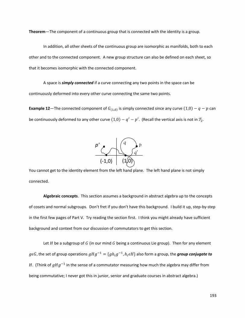
193

Theorem—The component of a continuous group that is connected with the identity is a group.

In addition, all other sheets of the continuous group are isomorphic as manifolds, both to each

other and to the connected component. A new group structure can also be defined on each sheet, so

that it becomes isomorphic with the connected component.

A space is simply connected if a curve connecting any two points in the space can be

continuously deformed into every other curve connecting the same two points.

Example 12—The connected component of ( ) is simply connected since any curve ( ) can

be continuously deformed to any other curve ( ) (Recall the vertical axis is not in

You cannot get to the identity element from the left hand plane. The left hand plane is not simply

connected.

Algebraic concepts. This section assumes a background in abstract algebra up to the concepts

of cosets and normal subgroups. Don’t fret if you don’t have this background. I build it up, step-by-step

in the first few pages of Part V. Try reading the section first. I think you might already have sufficient

background and context from our discussion of commutators to get this section.

Let be a subgroup of (in our mind being a continuous Lie group). Then for any element

the set of group operations { } also form a group, the group conjugate to

. (Think of in the sense of a commutator measuring how much the algebra may differ from

being commutative; I never got this in junior, senior and graduate courses in abstract algebra.)

(1,0)

p

q'

q

(-1,0)

p'

194

Example 13—The one-dimensional subgroup of ( ) (the right hand half-plane of example 1) given by

( ) gives rise to the series of conjugate groups

( )( )( ) ( )( ) ( ) (

)

( ) ( ( ))

You can check the group axioms to confirm that the subset of group elements ( ( ))

generated by conjugation is indeed a subgroup of corresponding to ( ) The subgroup conjugate to

the abelian group ( ) is

( )( )( ) ( )

Every element in this conjugate subgroup is in the original subgroup. We signify this by writing

Subgroups that are self-conjugate for all elements of are called invariant

subgroups or normal subgroups. The subgroup ( ) is an abelian invariant subgroup

Theorem—The connected component of a continuous group is an invariant subgroup of

(Welcome to some algebraic topology.)

Example 14—The right hand half-plane ( )

If is a subgroup of ( ), the structure are called cosets. A right coset is the set of

group operations ( reads such that)

where no element is contained in more than once in the sum above as if The

right (and left) cosets are disjoint. In another way of saying it, every element can be written

uniquely (!)

195

Analogously, left cosets involve a ! decomposition

Notation: A subgroup of is denoted by If it is a proper subgroup denoted by

Example 15—Let ( ) ( ) ( ) (Geometrically, is the

line ( ) lying on the axis; is a vertical line from to situated at )

( ) ( ) (

)

We can read this equation in two ways: ( ) since ( ) and (

) or

( ) since ( ) and (

) Draw pictures to better see this! It also

never hurts to check things. Let’s check

( )( )( ) ( )( ) (

) ( ) (

)

( ) ( )

Theorem—Left and right cosets of a continuous group by a closed subgroup of are manifolds

of dimension (Wow).

I offer no proof here, but I do provide an example. We have

( )

( )

196

Theorem—If is an invariant (normal) subgroup of then the coset elements can be chosen

in such a way that they are closed under multiplication and form a group called the factor group

Note that is not an invariant subgroup of yet is a group. Accidents like this can happen. On

the other hand and the theorem above guarantees that is a group, a factor group.

Example 16—The connected component of ( ( )) is an invariant (normal) subgroup. Every element

of can be written, for example, as either

(

) (

)

( ) (

) (

)

The coset representatives consist of one element from each sheet. This is not the most clever

choice (an art) for coset representations. A better choice would be ( ) and ( ) This

forms a closed group (⟨ ⟩) since ( ) ( ) ( ) ( ) ( )( ) ( )

( )( ) Generally, a good choice for coset representatives for the factor group

would be the element in each sheet that becomes the identity under the mapping that turns that sheet

into a group isomorphic ( ) with the connected component. Let’s illustrate this. A many sheeted

continuous group can be written as the sum of group operations of the form

⋃

where the and is the connected component. Each sheet is topologically equivalent as a

manifold. Only can be made isomorphic with the subgroup by acting with on the left.

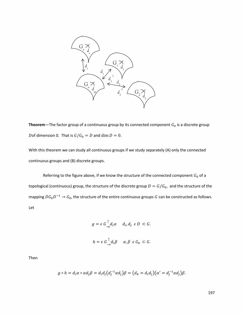
197

Theorem—The factor group of a continuous group by its connected component is a discrete group

of dimension 0. That is and

With this theorem we can study all continuous groups if we study separately (A) only the connected

continuous groups and (B) discrete groups.

Referring to the figure above, if we know the structure of the connected component of a

topological (continuous) group, the structure of the discrete group , and the structure of the

mapping the structure of the entire continuous groups can be constructed as follows.

Let

Then

( ) ( )(

)

d1

-1

Go d

o

G1 d

1

G2 d

2

Go d

o

do

d1

d2

-1

d2

198

Since has a group structure, the product Since is an invariant (normal) subgroup ,

Therefore, the group multiplication properties in the discrete factor group and in the

connected continuous component , together with the mapping uniquely determine

the group multiplication properties of the entire group

Let the elements of the discrete group be and let be the

sheet containing Then the sheet containing the identity is the connected component The

mapping that converts any sheet (which cannot be a group unless ) into a group isomorphic with

is given by

See the figure above for this process.

The invariant integral. The study of functions defined on the group manifold require the use

of an integral function defined over the group elements. The rearrangement property. The operation of

multiplication by a group element may be interpreted either as a mapping of the entire topological

group onto itself, or as a change of basis within the topological space. If ( ) is any scalar-valued

function defined on the group (or equivalently on the topological space ) then a reasonable

requirement for a group integral is

∫ ( ) ( ) ∫ ( ) ( ) ∫ ( ) ( )

This is reasonable because if the sum over involves each exactly once, the sum over involves

each group operation also exactly once (in a scrambled order). Since is an arbitrary function, we

demand of the measure defined on the group that it obey

( ) ( )

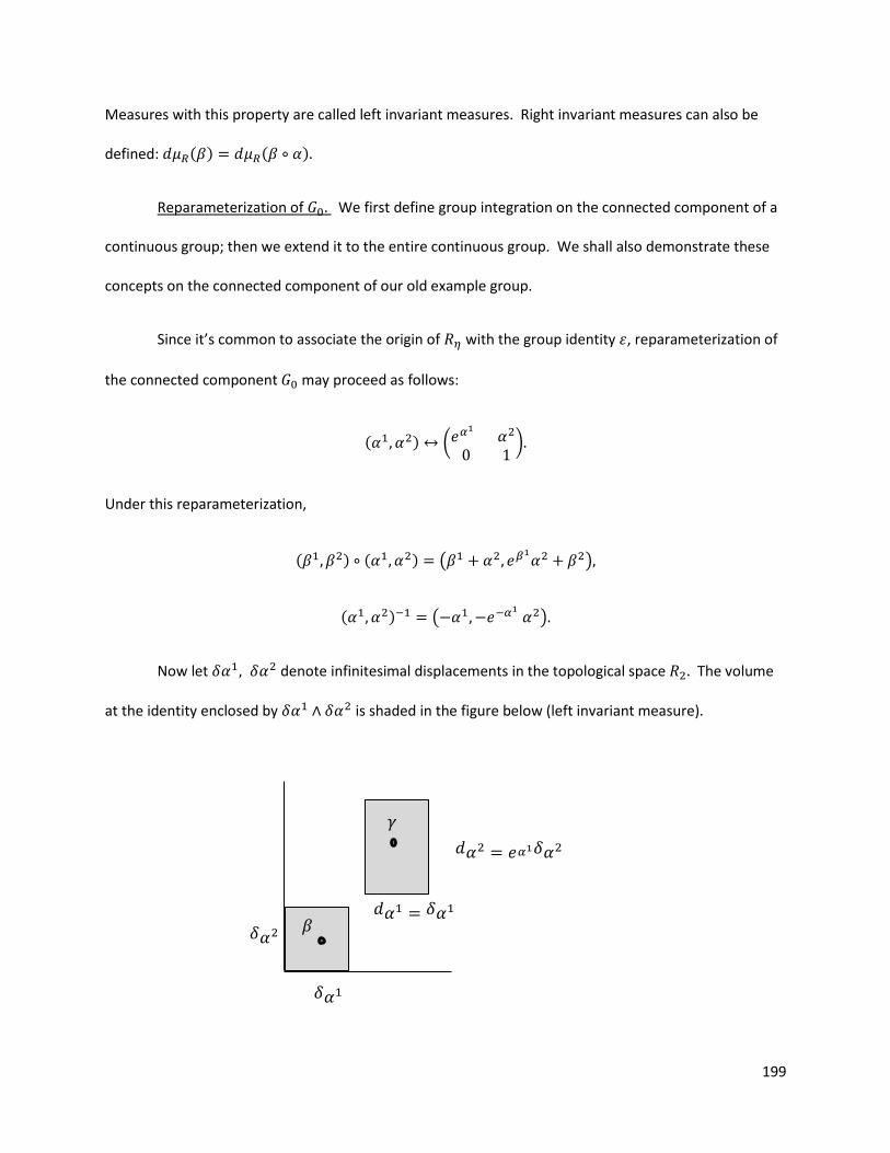
199

Measures with this property are called left invariant measures. Right invariant measures can also be

defined: ( ) ( )

Reparameterization of We first define group integration on the connected component of a

continuous group; then we extend it to the entire continuous group. We shall also demonstrate these

concepts on the connected component of our old example group.

Since it’s common to associate the origin of with the group identity , reparameterization of

the connected component may proceed as follows:

( ) (

)

Under this reparameterization,

( ) ( ) ( )

( ) ( )

Now let denote infinitesimal displacements in the topological space The volume

at the identity enclosed by is shaded in the figure below (left invariant measure).

𝛿𝛼

𝛿𝛼

𝛾

𝑑𝛼 𝛿𝛼

𝑑𝛼 𝑒𝛼 𝛿𝛼

𝛽

200

Let’s fill in the details for the left invariant measure.

( ) ( ) ( ) ( )

( ) ( ) ( ) ( )

Since then There is no change of scale alone the axis. On the other

hand,

( ) ( ) ( )

So The transformed rectangle is stretched along the axis. Then the volume element

( )

What about the right invariant measure?

( ) ( ) ( ) ( )

( ) ( ) ( ) (

)

So again and Now,

( ) ( ) ( ) ( )

So This seems right, but it is not what the source author concluded. (Shenanigans are

afoot.) Here is what probably makes the most sense for extracting these deltas the right way. Do it all in

one shot. (Doing it in pieces might get you lucky—the right results.)

( ) ( ) ( )

We get . Expand the exponential to first order, and So

Fixing crap like this over spans of years and books is wasted time.

201

Let be any point infinitesimally near to the identity and within the volume element as we

have shown in the figure for left invariant measure (and our imaginary picture for right invariant

measure). Under translation by ( ) the volume element ( ) around expands as it is moved

to a volume element ( ) around The coordinates of any point ( ) may be expanded

as

( ) ( ) ( ) ( )

⌉

The Euclidean volume element ( ) expands as it is moved around by the factor

( ) ( ) ( ) ( ) ( )

(For the reader who has notice the operator I’m pretty sure the source author is thinking in terms of

differential forms. We’re okay thinking of it as a simple product in this work). Therefore we should

weigh the Euclidean volume element in the vicinity of by a factor to preserve volume invariance

over the entire topological space:

For the right translation by we have, analogously,

( ) ( ) ( ) ( ) ( )

We dropped because this is a 2nd order term. Evidently then, the right invariant integral is

defined by a uniform density, whereas the left invariant density is nonuniform, defined by

General right and left invariant densities. We now turn to the general case. Let

be infinitesimal displacement n the independent directions of at the identity

element 0. The volume they enclose is give by

202

( ) ( )

Move this volume element to an arbitrary element ( ) to an arbitrary group element by

left translation, and demand of the density function that

( ) ( ) ( )

Here ( ) is the Euclidean volume element ( ) after it has been moved from the vicinity of (0) to

the vicinity of ( ) by left translation with It is easy to compute

( )

( ) ( ) ( ) ( )

|

Then we have

( ) ( )

|

( )

|

‖

( )

‖

( )

The density for left translations must thus satisfy ( ( ) )

( ) ‖ ( )

‖

Doing all of the above for the right leads to

( ) ‖ ( )

‖

These invariant densities are Haar measures.

203

Equality of left and right measures. The left and right measures computed in our previous

figure were not equal. Furthermore, the integrals

∫ ( ) ( ) ∫ ( ) ( )

for our example do not converge (though any integral ∫ ( ) ( ) ( )

which did converge would be invariant. Where are the left and right measures equal? And we do they

converge?

Theorem—The density functions ( ) and ( ) giving the left and right invariant measures of

compact group are equal.

Proof. Begin with an element of volume ( ) at the identity of the group operation. Move this

element to an invariant volume at by left translation. The result is

( ) ( ) ( )

If we now move this invariant volume back to the identity using right translation by , the result is a

volume element at the identity, but with a possibly different size and shape. The left translation

mapped a rectangle to a rectangle with the same orientation, but the right translation, had I drawn it,

results in mapping a rectangle to a rotated parallelogram. Mathematically we have:

[ ( ) ( ) ( ) ( ) ( )

( ) [ ( ) ( )] ( )

( ) ( ) ( )

Then define recursively

204

( ) ( ) ( ) ( ) ( )

( ) ( ) ( ) ( ) ( )

Since the group is compact (and every sequence has a convergent subsequence) the limit as

exists and is well defined: ( ) and

( )

( )( )

[ ( )] ( ) ( ) ( )

If ( ) then

[ ( )] is infinity for the > case and 0 for the < case. But since is an element of

the group, ( ) can be neither 0 nor infinity, for then the operation ( ) would be singular.

We are forced to conclude that ( ) , thus ( ) ( ) and ( ) ( ) The left and

right measures on a compact group are equal.

Note from source author: The left and right measures equal on the following kinds of groups:

1. Finite groups.

2. Discrete groups.

3. (Locally compact) abelian groups.

4. Compact groups.

5. Simple groups.

6. Semisimple groups.

7. Real connected algebraic groups with determinant +1.

8. Connected nilpotent Lie groups.

9. Semidirect product groups such as ( ) or ( ) Poincaré groups ( ) or

ISO(3,1).

10. Constructions of semisimple groups by maximal subgroups: ( ) ( ) ( )

11. Lie groups for which ( ) is unimodular.

205

Extension to continuous groups. The invariant integrals have so far been built for the connected

components of a continuous group. To extend to the other sheets we need to observe two things.

1. Every element can be written as where a discrete factor group, and

the connected component. 2. Each sheet is topologically equivalent to every other sheet.

The required extension is then

∫ ( ) ( ) ( )

∑ ∫ ( ) ( ) ( )

If it happens that the connected component is of dimension zero, it contains only one point, the identity

and the invariant integral reduces to (with ( ) ) to the form familiar for discrete groups:

∫ ( ) ( ) ( ) ∑ ( )

Done on this.

Part III were my notes from Gilmore’s text, specifically from chapters 3 and 4, interspersed with

filled in steps and underlying physical motivations. The first two chapters are worth a read, especially

the stuff dealing with metrics. Three more blocks of ideas remain regarding symmetry methods.

Chapters 1-4 of Jones’ text develop the mathematics of discrete groups (our focus has been primarily on

continuous groups, but not exclusively). We learn how to create characteristic tables for discrete

groups. You connect these practical results with the first chapter of Gilmore’s 2008 text and you have a

proof of Galois’ work on the insolvability of the quintic by radicals. I never got it from crappy formal

training overloaded with blinding abstraction. These cover the first two of the remaining blocks.

206

Is the quintic really unsolvable? Yes. By radical extensions. Galois showed us this. But

mathematicians have built a mathematical technology, if you will, to get around the limitations of

solvability by radicals. They have built on the theory of elliptic functions and elliptic integrals to deal

with questions of solvability. I only know one elliptic integral well. It arises from the study of the

pendulum for larger angles, where one can’t use the Taylor approximation Find impossibility.

Find workaround. Be water my friend. Can’t trisect an angle, double the cube, square the circle? Get

the hell out of here! Go pick up something more than a straightedge and compass. C’mon. There are

pathologies with vector (or gauge) potentials. Workaround. Connections over principle bundles. The

best step-by-step book treating connections on bundles is “Geometry, Topology and Physics,” M.

Nakahara, Institute of Physics Publishing, 1990. The relevant material is in chapters 9 and 10, which I

found I could jump into without reading prior chapters. The early chapters, however, are worth a read,

especially on homology and homotopy. I understand there is a second edition. The book, “Topology,

Geometry and Gauge Fields,” by G. L. Naber, Springer 1997, I found impenetrable. Yet Naber does do a

good job of connecting the mathematics to the physics at the word level, feeding my understanding.

This material is drier—apologies.

Assuming that you have a junior level background in quantum mechanical addition of angular

momentum, the final block on algebra is COMPLETELY SELF CONTAINED In FULL DETAIL. You will study

Addition of Angular Momentum in terms of tensor products and direct products matrix methods, ladder

operators and Young’s tableaux. We will cover SU(2) for electron spin and Isospin and SU(3) for the

quarks u, d and s. As a useful aside yielding selection rules, we will present in FULL DETAIL the

application of the Wigner-Eckart theorem applied to scalars and vectors, and then extend the results to

tensors. You may skip this if you’re more interested in particle physics such as the Standard Model and

its extensions to Grand Unified Theories (GUTs) and Theories of Everything (TOEs). What you will learn

for SU(2) and SU(3) will be generalized in terms of the Cartan subalgebra with attendant ladder

207

operators, root and weight diagrams and Dynkin diagrams so that the 2nd half of Jones is becomes much

more readable, and so that you might have some chance of working through trash like Georgi’s book on

Lie algebras and particle physics.

Part IV. (The first six pages quickly review sophomore algebra.) We’ve just finished seeing the

algebraic topology of continuous groups in terms of cosets and invariant (or normal) subgroups. Here

are their discrete versions. Consider the symmetries of an equilateral triangle on the plane.

We may rotate by , the identity operation We may rotate to the left by We may rotate

left by We may reflect the left diagonal We may reflect about the right diagonal We

may reflect about the vertical diagonal These operations lead to finite, discrete group with table:

208

The element is a (proper) subgroup of as are the elements { } There are no other

proper subgroups. We write where is the dihedral group of the triangle, is the

cyclic group of the triangle, and is the trivial subgroup. (A cyclic group is any group generated by a

single element; for the triangle we could pick to be the generator as )

The subgroup has the following one-dimensional representation

( ) ( ) ( )

These are dimensional unitary matrices. Each of these matrices is irreducible (so, peeking ahead,

( ) ( ) ( ); note that ; this will have meaning).

Conjugacy. are conjugate if there exists ( ) We call the

conjugating element (fun) and we write . (Back in continuous groups this is the commutator, a

measuring device indicating how much the group deviates from being commutative (abelian).)

Conjugacy classes. [ ] { | } This reads, the conjugacy class of is the set of all that

are equivalent to (It’s tacit that The tilde denotes equivalence relation.

For each element is a conjugacy class, as is the case for all abelian groups;

for some For we have three conjugacy classes: [ ] [ ] [ ]

Certainly Check all the cases, i.e., and so on.

In terms of matrices, the group elements are represented by

(

)

( √

√ )

( √

√ )

( √

√ )

( √

√ ) (

)

209

The subgroup is represented by the first three of these six matrices. The dimension of a

representation is the dimension of the space on which it acts. We have seen both a one-dimensional

representation of and a two-dimensional representation. When we define the regular

representation, we will see that it is three-dimensional for , with a concomitant geometric picture,

and that for the regular representation is six-dimensional. The dimensionality of the regular

representation will be the size of the group. (Note: This is sophomore/junior level modern algebra. The

pace will be fast through these basics.)

Left (right) cosets. Given a subgroup the left cosets are { } (or { } for right cosets).

Lagrange’s Theorem—If is a subset of ( ), then [ ]|[ ] (read the order of divides

the order of (The proof is sophomore modern algebra.)

Example 1—[ ]|{ ] | Three divides six equaling two. Another notation is

Normal subgroup. If we say is a normal (invariant) subgroup of ( ) if

Example 2— Let’s check. I’ll be abusive with notation to cut the work down. Pick any element

from each of the three sets and will get { } { } { }

{ } This is also

true for { }{ }{ } { }

There are two additional groups you should be aware of, the permutation group and the

alternating group Depending on the author, you will find the multiplication rule of these groups

reversed—it’s confusing. Here is an element of the permutation group on three symbols:

(

)

The symbols 2 and 3 have been exchanged. An example multiplication of two members of is

210

(

) (

) (

) ( )

The (1 2) notation is called cycle notation. I started on the right parenthesis, noting that 3 goes to 2,

then in the left parenthesis, 2 goes to 3; so 3 remains unaffected. Then we go back to the right

parenthesis to see that 2 goes to 1, then over to the left parenthesis to see that 1 goes to 1. So,

effectively 2 goes to 1. Then lastly, from the right parenthesis I see that 1 goes to 3, over to the left

parenthesis to see that 2 goes to 2. Thus 1 goes to 2. The shorthand cycle notation captures this group

multiplication succinctly with (1 2); 1 goes to 2; 2 goes to 1; 3 remains unchanged. Given three symbols

{1,2,3}, we know there are 3!=6 permutations, thus is a group of order 3. The alternating group on n

symbols, is the group of even permutations of has

elements. Example of an odd

permutation

(

) ( )( )( )

We cannot express the group element on the left by an even number of 2-cycles, e.g., (1 5). Had the

group element been expressible by an even number of 2-cylces it would have been an even

permutation, and a member of We trouble about these because of the following theorem.

Cayley’s Theorem—Every finite group is isomorphic to a subgroup of That is

∏( ) (

)

There is a sophomore level proof I’ll level to an introductory book.

Quotient group (Factor group). Let me first give you an example using Let

{ } and let { }. Observe that and form a group:

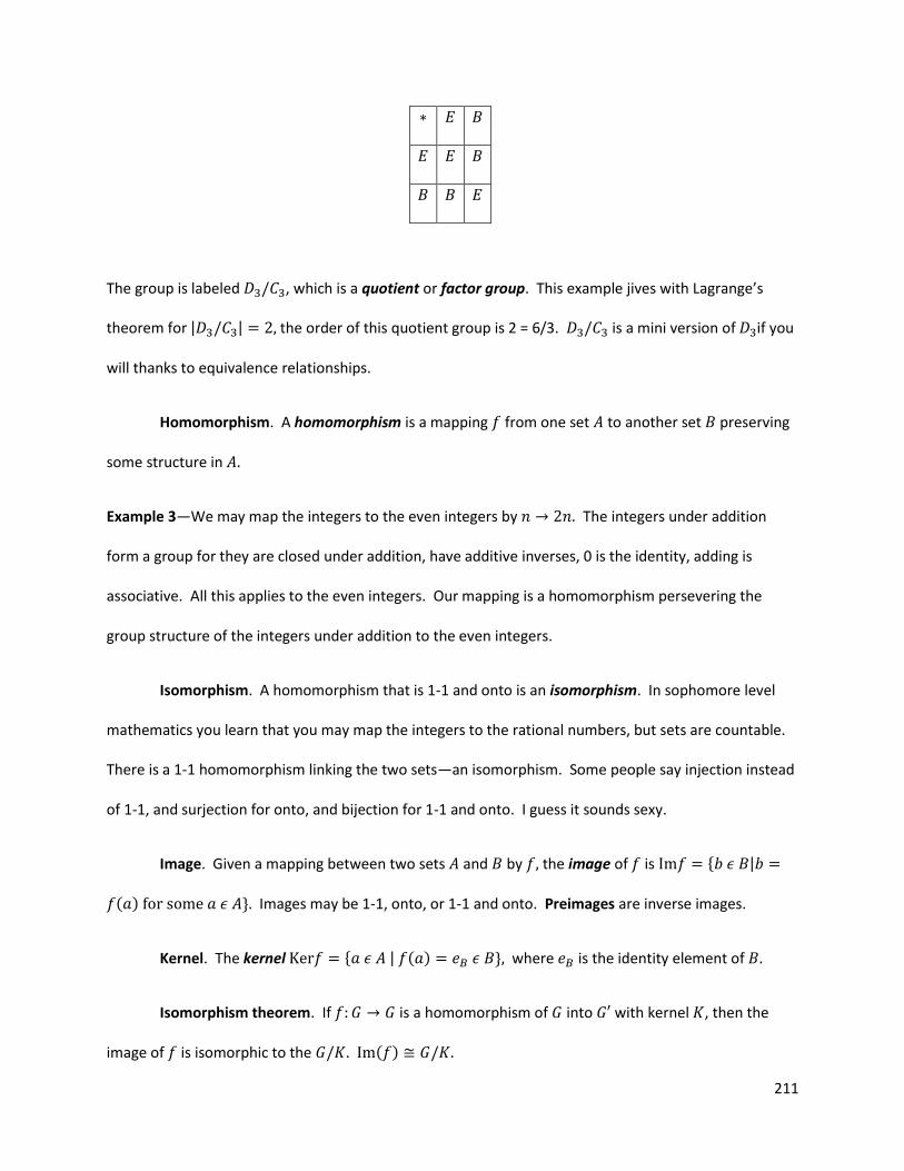
211

The group is labeled , which is a quotient or factor group. This example jives with Lagrange’s

theorem for | | the order of this quotient group is 2 = 6/3. is a mini version of if you

will thanks to equivalence relationships.

Homomorphism. A homomorphism is a mapping from one set to another set preserving

some structure in

Example 3—We may map the integers to the even integers by The integers under addition

form a group for they are closed under addition, have additive inverses, 0 is the identity, adding is

associative. All this applies to the even integers. Our mapping is a homomorphism persevering the

group structure of the integers under addition to the even integers.

Isomorphism. A homomorphism that is 1-1 and onto is an isomorphism. In sophomore level

mathematics you learn that you may map the integers to the rational numbers, but sets are countable.

There is a 1-1 homomorphism linking the two sets—an isomorphism. Some people say injection instead

of 1-1, and surjection for onto, and bijection for 1-1 and onto. I guess it sounds sexy.

Image. Given a mapping between two sets and by the image of is { |

( ) } Images may be 1-1, onto, or 1-1 and onto. Preimages are inverse images.

Kernel. The kernel { | ( ) } where is the identity element of

Isomorphism theorem. If is a homomorphism of into with kernel , then the

image of is isomorphic to the ( )

212

Think about this, if the kernel , the identity element, the order of { } is one, and by

Lagrange’s theorem, | | | | | | So the mapping is 1-1. and are the same size and have the

same algebra. They are different only in as much their symbology is different, e.g., matrix

representations versus analytic realizations.

Up to this point, we have the minimum algebra we need to proceed. If these definitions and

theorems become fuzzy, review the triangle group or whip out the square and work out its group

structure, then check the theorems with concrete examples. We begin the Jones notes. Think of group

representations in terms of matrix representations.

A representation of dimension of a group is defined by

( ) where are an

nonsingular complex matrices. IMPORTANT. Two [ ] representations ( ) ( ) of a group are

equivalent (~) if ( )( ) ( )( ) This is a similarity

transformation

( )( ) ( )( ) ( )( )

Thus

( )( ) ( ) ( )( ) ( )( ) ( )( ) ( ( ) )( ( )( ) )

( )( ) ( )( ) ( )( )

Example 4—In quantum mechanics one often seeks to diagonalize a matrix (change its basis to a

diagonal basis) by similarity transformation. Consider

(

)

The trace of the matrix is 2. The determinant is 0. This gives us two constraints on the eigenvalues.

213

Here is something that fits the constraints: We could have proceeded with

more traditional matrix algebra:

|

| ( )( ( ) )

The resulting polynomial is ( ) The roots are { } For each root, we then

find the eigenvalues as follows. Pick eigenvalue 2.

(

)(

) (

)

Working this out means

(

) (

)

This can only be so if and Keeping it simple, let Then indeed

(

)( ) (

)

The eigenvector is an eigenstates of the physical system. In quantum mechanics eigenstates are

normalized to 1 because of its probabilistic interpretation. The dot product (or length) of the

eigenstates is

( ) ( )

So let the normalized eigenvector be

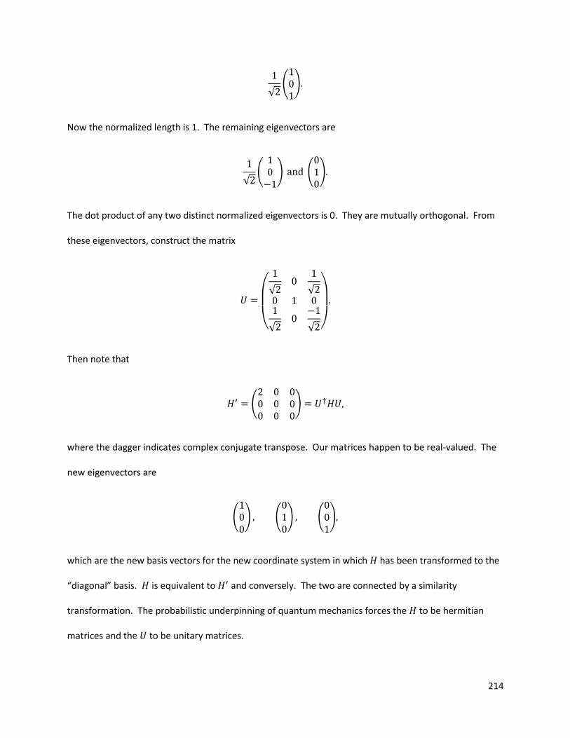
214

√ ( )

Now the normalized length is 1. The remaining eigenvectors are

√ (

) ( )

The dot product of any two distinct normalized eigenvectors is 0. They are mutually orthogonal. From

these eigenvectors, construct the matrix

(

√

√

√

√ )

Then note that

(

)

where the dagger indicates complex conjugate transpose. Our matrices happen to be real-valued. The

new eigenvectors are

( ) (

) (

)

which are the new basis vectors for the new coordinate system in which has been transformed to the

“diagonal” basis. is equivalent to and conversely. The two are connected by a similarity

transformation. The probabilistic underpinning of quantum mechanics forces the to be hermitian

matrices and the to be unitary matrices.

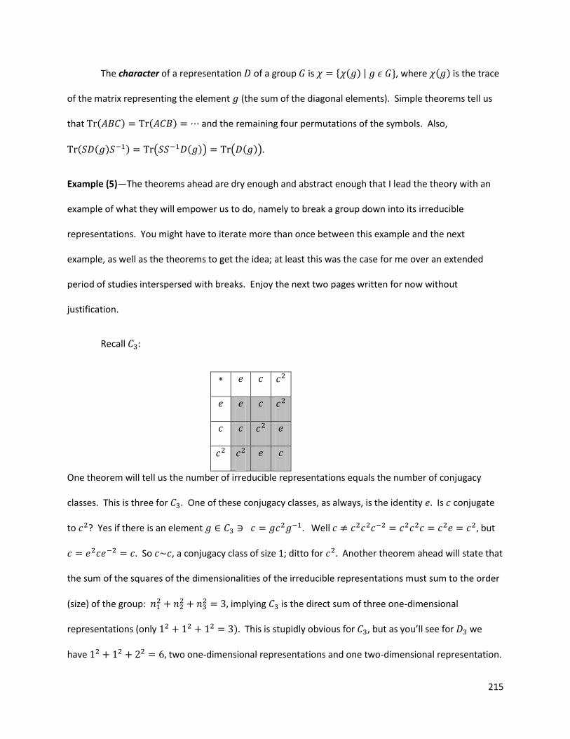
215

The character of a representation of a group is { ( ) | }, where ( ) is the trace

of the matrix representing the element (the sum of the diagonal elements). Simple theorems tell us

that ( ) ( ) and the remaining four permutations of the symbols. Also,

( ( ) ) ( ( )) ( ( ))

Example (5)—The theorems ahead are dry enough and abstract enough that I lead the theory with an

example of what they will empower us to do, namely to break a group down into its irreducible

representations. You might have to iterate more than once between this example and the next

example, as well as the theorems to get the idea; at least this was the case for me over an extended

period of studies interspersed with breaks. Enjoy the next two pages written for now without

justification.

Recall

One theorem will tell us the number of irreducible representations equals the number of conjugacy

classes. This is three for . One of these conjugacy classes, as always, is the identity Is conjugate

to ? Yes if there is an element Well but

So , a conjugacy class of size 1; ditto for Another theorem ahead will state that

the sum of the squares of the dimensionalities of the irreducible representations must sum to the order

(size) of the group:

implying is the direct sum of three one-dimensional

representations (only ) This is stupidly obvious for , but as you’ll see for we

have two one-dimensional representations and one two-dimensional representation.

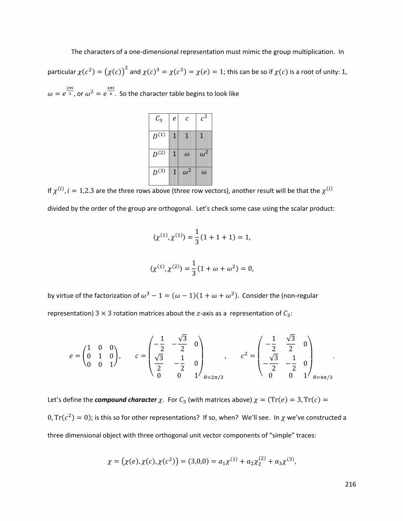
216

The characters of a one-dimensional representation must mimic the group multiplication. In

particular ( ) ( ( ))

and ( ) ( ) ( ) ; this can be so if ( ) is a root of unity: 1,

or

So the character table begins to look like

( ) 1 1 1

( ) 1

( )

If ( ) are the three rows above (three row vectors), another result will be that the ( )

divided by the order of the group are orthogonal. Let’s check some case using the scalar product:

⟨ ( ) ( )⟩

( )

⟨ ( ) ( )⟩

( )

by virtue of the factorization of ( )( ) Consider the (non-regular

representation) rotation matrices about the -axis as a representation of :

(

)

(

√

√

)

(

√

√

)

Let’s define the compound character . For (with matrices above) ( ( ) ( )

( ) ); is this so for other representations? If so, when? We’ll see. In we’ve constructed a

three dimensional object with three orthogonal unit vector components of “simple” traces:

( ( ) ( ) ( )) ( ) ( )

( ) ( )

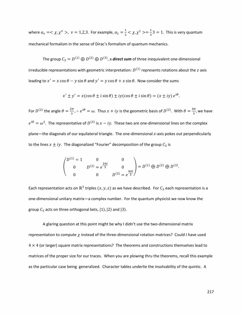
217

where For example,

This is very quantum

mechanical formalism in the sense of Dirac’s formalism of quantum mechanics.

The group ( ) ( ) ( ) a direct sum of three inequivalent one-dimensional

irreducible representations with geometric interpretation: ( ) represents rotations about the axis

leading to and Now consider the sums

( ) ( ) ( )

For ( ) the angle

Thus is the geometric basis of ( ) With

we have

The representative of ( ) is These two are one-dimensional lines on the complex

plane—the diagonals of our equilateral triangle. The one-dimensional -axis pokes out perpendicularly

to the lines . The diagonalized “Fourier” decomposition of the group is

(

( )

( )

( )

) ( ) ( ) ( )

Each representation acts on triples ( ) as we have described. For each representation is a

one-dimensional unitary matrix—a complex number. For the quantum physicist we now know the

group acts on three orthogonal kets, | ⟩ | ⟩ and | ⟩.

A glaring question at this point might be why I didn’t use the two-dimensional matrix

representation to compute instead of the three-dimensional rotation matrices? Could I have used

(or larger) square matrix representations? The theorems and constructions themselves lead to

matrices of the proper size for our traces. When you are plowing thru the theorems, recall this example

as the particular case being generalized. Character tables underlie the insolvability of the quintic. A

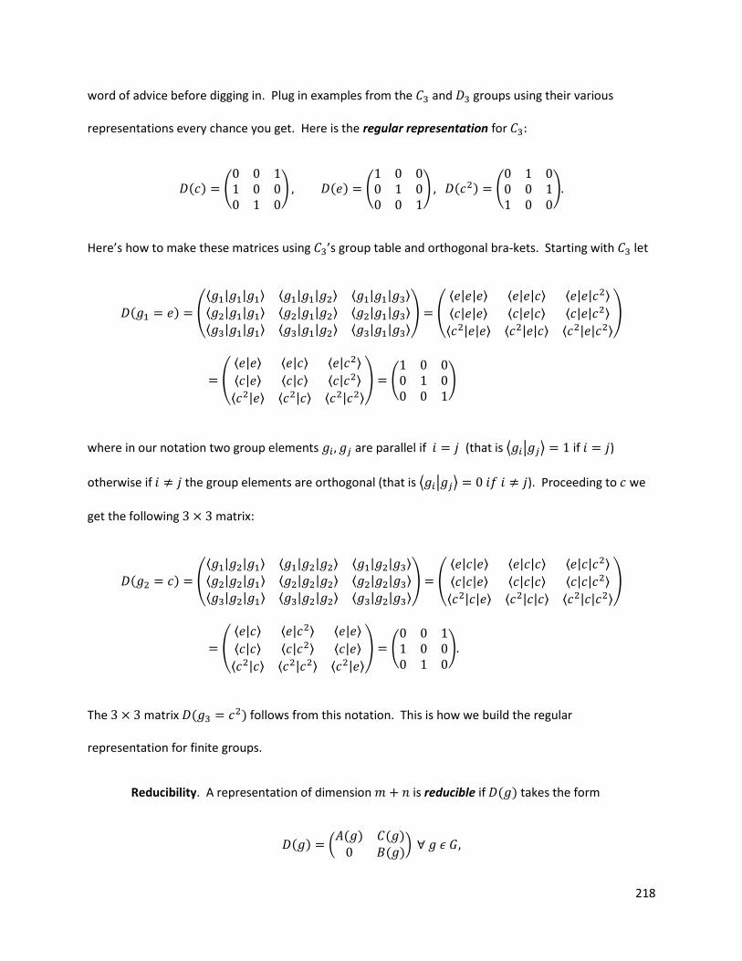
218

word of advice before digging in. Plug in examples from the and groups using their various

representations every chance you get. Here is the regular representation for

( ) (

) ( ) (

) ( ) (

)

Here’s how to make these matrices using ’s group table and orthogonal bra-kets. Starting with let

( ) (

⟨ | | ⟩ ⟨ | | ⟩ ⟨ | | ⟩

⟨ | | ⟩ ⟨ | | ⟩ ⟨ | | ⟩

⟨ | | ⟩ ⟨ | | ⟩ ⟨ | | ⟩) (

⟨ | | ⟩ ⟨ | | ⟩ ⟨ | | ⟩

⟨ | | ⟩ ⟨ | | ⟩ ⟨ | | ⟩

⟨ | | ⟩ ⟨ | | ⟩ ⟨ | | ⟩

)

(

⟨ | ⟩ ⟨ | ⟩ ⟨ | ⟩

⟨ | ⟩ ⟨ | ⟩ ⟨ | ⟩

⟨ | ⟩ ⟨ | ⟩ ⟨ | ⟩

) (

)

where in our notation two group elements are parallel if (that is ⟨ | ⟩ if )

otherwise if the group elements are orthogonal (that is ⟨ | ⟩ ). Proceeding to we

get the following matrix:

( ) (

⟨ | | ⟩ ⟨ | | ⟩ ⟨ | | ⟩

⟨ | | ⟩ ⟨ | | ⟩ ⟨ | | ⟩

⟨ | | ⟩ ⟨ | | ⟩ ⟨ | | ⟩) (

⟨ | | ⟩ ⟨ | | ⟩ ⟨ | | ⟩

⟨ | | ⟩ ⟨ | | ⟩ ⟨ | | ⟩

⟨ | | ⟩ ⟨ | | ⟩ ⟨ | | ⟩

)

(

⟨ | ⟩ ⟨ | ⟩ ⟨ | ⟩

⟨ | ⟩ ⟨ | ⟩ ⟨ | ⟩

⟨ | ⟩ ⟨ | ⟩ ⟨ | ⟩

) (

)

The matrix ( ) follows from this notation. This is how we build the regular

representation for finite groups.

Reducibility. A representation of dimension is reducible if ( ) takes the form

( ) ( ( ) ( ) ( )

)

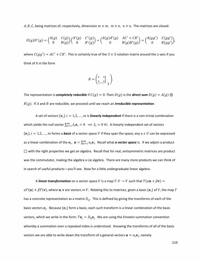
219

being matrices of, respectively, dimension The matrices are closed:

( ) ( ) ( ( ) ( ) ( )

) ( ( ) ( )

( )) (

( ) ( )

( ) ( )) (

( ) ( )

( ))

where ( ) This is certainly true of the rotation matrix around the -axis if you

think of it in the form

(

|

)

The representation is completely reducible if ( ) Then ( ) is the direct sum ( ) ( )

( ) If and are reducible, we proceed until we reach an irreducible representation.

A set of vectors { } is linearly independent if there is a non-trivial combination

which yields the null vector ∑ A linearly independent set of vectors

{ } forms a basis of a vector space if they span the space; any can be expressed

as a linear combination of the , ∑ Recall what a vector space is. If we adjoin a product

with the right properties we get an algebra. Recall that for real, antisymmetric matrices are product

was the commutator, making the algebra a Lie algebra. There are many more products we can think of

in search of useful products—you’ll see. Now for a little undergraduate linear algebra.

A linear transformation on a vector space is a map such that ( )

( ) ( ) where are vectors in Relating this to matrices, given a basis { } of the map

has a concrete representation as a matrix This is defined by giving the transforms of each of the

basis vectors . Because { } form a basis, each such transform is a linear combination of the basis

vectors, which we write in the form: We are using the Einstein summation convention

whereby a summation over a repeated index is understood. Knowing the transforms of all of the basis

vectors we are able to write down the transform of a general vectors namely

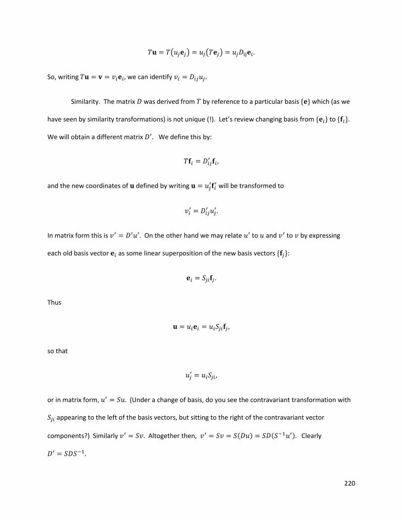
220

( ) ( )

So, writing we can identify

Similarity. The matrix was derived from by reference to a particular basis { } which (as we

have seen by similarity transformations) is not unique (!). Let’s review changing basis from { } to { }.

We will obtain a different matrix We define this by:

and the new coordinates of defined by writing

will be transformed to

In matrix form this is On the other hand we may relate to and to by expressing

each old basis vector as some linear superposition of the new basis vectors { }:

Thus

so that

or in matrix form, (Under a change of basis, do you see the contravariant transformation with

appearing to the left of the basis vectors, but sitting to the right of the contravariant vector

components?) Similarly Altogether then, ( ) ( ) Clearly

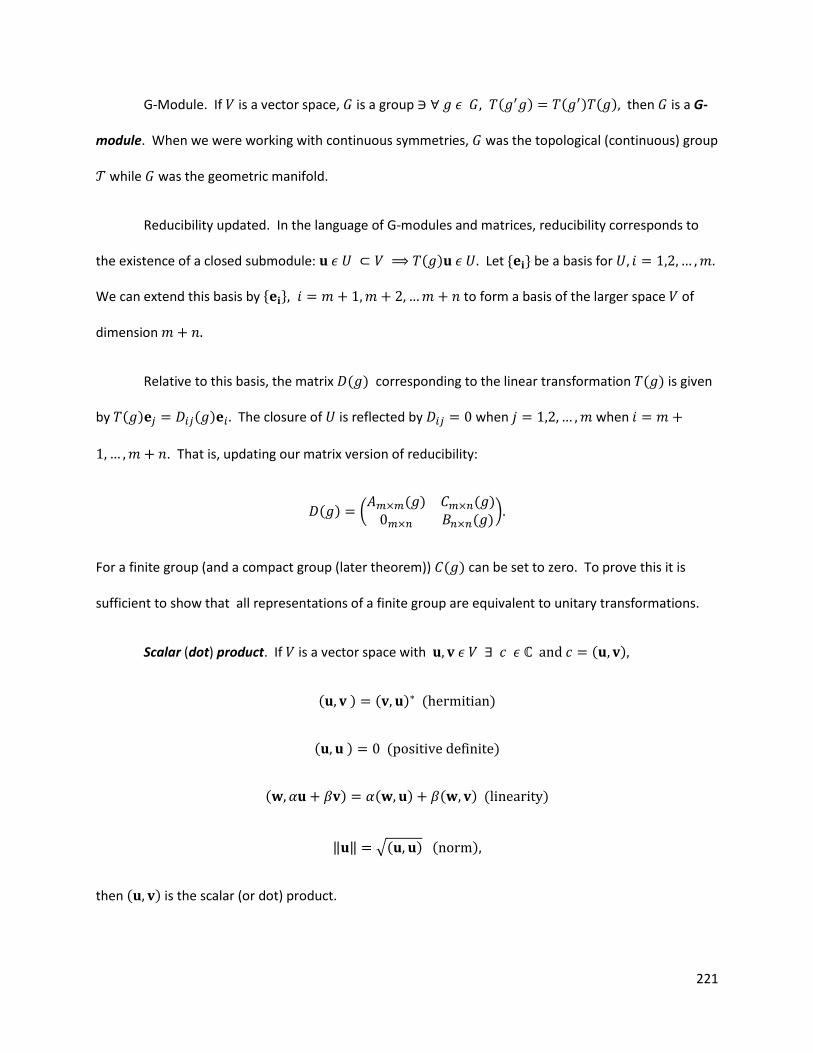
221

G-Module. If is a vector space, is a group ( ) ( ) ( ) then is a G-

module. When we were working with continuous symmetries, was the topological (continuous) group

while was the geometric manifold.

Reducibility updated. In the language of G-modules and matrices, reducibility corresponds to

the existence of a closed submodule: ( ) Let { } be a basis for

We can extend this basis by { } to form a basis of the larger space of

dimension

Relative to this basis, the matrix ( ) corresponding to the linear transformation ( ) is given

by ( ) ( ) The closure of is reflected by when when

. That is, updating our matrix version of reducibility:

( ) ( ( ) ( )

( ))

For a finite group (and a compact group (later theorem)) ( ) can be set to zero. To prove this it is

sufficient to show that all representations of a finite group are equivalent to unitary transformations.

Scalar (dot) product. If is a vector space with ( )

( ) ( ) ( )

( ) ( )

( ) ( ) ( ) ( )

‖ ‖ √( ) ( )

then ( ) is the scalar (or dot) product.

222

Orthonormal basis (ONB). Given any basis { } of a vector space it is possible to construct an

ONB { } ( ) The procedure is known as Gram-Schmidt orthogonalization:

‖ ‖

‖ ‖

‖ ‖

‖ ‖

Unitary transformations. A linear transformation acting in is unitary if ( )

( ) The ( ) are necessarily invertible if the transformation is unitary. Equivalently, we

can write

( ) ( )

and equivalently given relative to some ONB { }, we necessarily have ( ) For unitary

matrices ( ) the complex, conjugate equals the inverse. For a hermitian matrix,

Complete reducibility in terms of an ONB. Now that we have a scalar product, we may choose

the basis of to be an ONB. Any vector in the space spanned by the additional vectors { }

is orthogonal to any in

{ | ( ) }

In a coordinate-free language, complete reducibility corresponds to the closure of the subspaces and

under scalar product. This is always true if the ( ) are unitary transformations wrt to the scalar

product, for then

223

( ( ) ) ( ( ) )

The closure of then guarantees that ( ) ( ) Hence ( ( ) ) ( )

Cleary then ( )

Maschke’s Theorem. All reducible representations of a finite group are completely reducible—

decomposable into a direct sum of irreducible representations. (Hint: Use (cleverly create) a scalar

product which always gives us a unitary representation.)

Proof. Define the group invariant scalar product by building up from the original scalar

product, but now sum over all group elements:

{ }

[ ]∑( ( ) ( ) )

The { } are generic members of Consider { ( ) ( ) } The group invariant

scalar product becomes:

{ ( ) ( ) }

[ ]∑( ( ) ( ) ( ) ( ) )

[ ]∑( ( ) ( ) )

[ ]∑( ( ) ( ) )

Just as was true for group invariant left (right) measures for continuous groups, ∑ ∑ for discrete

groups. Thus we have

{ ( ) ( ) } { }

Evidently, the ( ) are unitary wrt to the group invariant scalar product which was cleverly created to

do exactly this. In terms of matrices, the ( ) will be realized as a reducible unitary matrix ( ) if we

224

choose a basis { } orthonormal wrt the group invariant scalar product, whose first members span

The ( ) will be related by the similarity transformation ( ) ( ) where is the matrix

effecting the change of basis from { } to { } (The representation is equivalent to the reducible

unitary representation which is completely reducible.) In pictures:

( |

| )

What does this group invariant scalar product look like for, say, ? Let ( ) and

( ) be vectors in The usual scalar product is

( ) ( ) ( ) (

)

With our three-dimensional rotation matrix representation, the group invariant scalar product looks like

[ ]∑( ( ) ( ) )

(

) [(

) ]

(

√

√

)

[

(

√

√

)

]

(

√

√

)

[

(

√

√

)

]

Schur’s first lemma. Any matrix which commutes with all the matrices of an irreducible

representation is a multiple of the identity,

( ) ( )

225

(Think in terms of the three matrices above.) In terms of linear operators,

( ) ( )

where is the linear operator version of and is the identity map

Proof. Let’s work with the linear operator version. Let be an eigenvector of with

eigenvalue : Then

( ( ) ) ( ) ( ) ( ( ))

Then ( ) is an eigenvector of with the same eigenvalue The space of all such eigenvectors is a

vector space which is a subset of the space It’s a -module, being closed under the linear operators

{ ( )}

By irreducibility, the only submodules are the space or the identity Since every linear

operator has at least one proper eigenvector, is not mapping vectors to the identity. In the complex

numbers, ( ) has at least one root corresponding to an eigenvector Thus the space of

eigenvectors of with eigenvalue is the whole space. So and as claimed.

Schur’s second lemma. Consider two inequivalent representations and In matrix form,

Schur’s second lemma states

( ) ( )

The corresponding linear operator will be a map between two vector spaces, each with two

different representations. In coordinate-free language, the equation above is

( ) ( )

226

where is the linear operator mapping every vector in onto the null vector in (

)

Before we get to the proof, what is this lemma telling us? We have two-dimensional

representations of (and ) and we have three-dimensional representations of these groups.

They are inequivalent representations. The only matrix that makes commute with matrices

is the operator above. This remains true for two inequivalent representations even if they have the

same dimensionality. Recall the one-dimensional irreducible representations of namely

( ) ( ) ( ). There is no nonzero (one-dimensional) matrix so that, say

Proof. Case (1). Suppose Consider the action of ( ) on an

arbitrary vector of From the above equation

( ) ( )

Since is a G-module, ( ) Thus,

( )( )

which means that is a submodule of But is, by supposition, irreducible. So must

be either the whole space or the null vector We can exclude the first case because we assumed

from the start that As the image of the dimension of of can’t exceed that of So

We’re left with

Case (2). If then the kernel of the mapping is

{ | }

227

The kernel is a submodule of since ( ( )) ) ( ) By the irreducibility of is either

the whole space or it is the null vector must be nontrivial because the images of of the

vectors of a basis of cannot all be linearly independent since the mapping is reducing the

dimensionality from to the smaller number Thus every vector must satisfy

Case (3). Let Again the kernel is a submodule of but it can’t be the null vector

because and are inequivalent. Recall what I said about the situation when the kernel is the identity

element, namely this means that the mapping is 1-1. We just assumed that and are inequivalent.

We conclude that

Physicist’s aside—at this point Georgi connects Schur’s lemmas with quantum physics.

Georgi’s version of Maschke’s theorem is that every representation of a finite group is completely

reducible. His proof involves the use of a projector operator such that ( ) ( )

(This is the condition that be an invariant subspace.) Georgi presses to a combined version of Schur’s

lemma: if ( ) ( ) where and are inequivalent irreducible representations,

then Then Georgi shows that Schur’s lemmas have strong consequences for the matrix elements

of any quantum mechanical operator that corresponds to an observable that is invariant under the

symmetry transformations. This is because the matrix elements ⟨ | | ⟩ behave like the in

Schur’s lemma. The details of this connection are shown from the middle of page 14 to the middle of

page 17 (2nd ed.). The rest of Georgi’s chapter 1 is in parallel with the Jones-based notes presented here

on finite groups, but using Dirac bra-ket notation and projection operators. End physicist’s aside.

Fundamental orthogonality theorem—with examples. Let and be two -modules

carrying inequivalent irreducible representations of some given group . (The indices may be

continuous for compact groups, but let’s let them be integers.) Pick an arbitrary linear mapping from

to and construct (yes we construct) the following operator

228

∑ ( )( ) ( )( )

This involves the same (scalar product) sum that was constructed to make ( )( ) unitary (under this

constructed scalar product). (For compact groups we replace the sum with ∫ ( ) review Part III.)

Let be any member of and consider

( )( ) ∑ ( )( ) ( )( ) ( )( )

Notice that this involves the same sum over group elements used in Maschke’s theorem. Thus,

( )( ) ∑ ( ) ( ) ( )( )

from the group property of the ( ). Let be Then the argument of ( ) becomes

and we know the sum over is the same as the scrambled sum over Thus

( )( ) ∑ ( )( ) ( )( ) ∑ ( )( ) ( )( )

from the group property of the ( ) Notice the first three factors, summed over give again. Thus

( )( ) ( )( )

Evidently satisfies the conditions of Schur’s second lemma; thus unless In the latter

case the two representatives are the same. Well then Schur’s first lemma applies, yielding

This can be expressed in matrix form as

∑ ( )( ) ( )( )

( )

229

The constant depends both on the label of the irreducible representation and on the choice of matrix

which remains unspecified. Let’s make life easy by specifying all elements of to be zero except for

So now write ( )

as Then the matrix element of the sum above reads

∑ ( )

( ) ( )( )

The ( )

can be found by setting and tracing (contracting with summation that is). This gives

∑( ( )( ) ( )( ))

( )

where is the dimensionality of ( ) The matrix ( )( ) ( )( ) is just the unit matrix with

matrix elements Thus [ ] ( )

Substituting for ( )

in ∑ ( )( ) ( )( )

( )

we obtain the fundamental orthogonality relation for the matrices of irreducible representations as the

equation below:

∑ ( )

( ) ( )( )

[ ]

What does ∑ ( )

( ) ( )( )

[ ]

look like? Is the result independent of the

matrix representation? Consider for example the two-dimensional representations of the

dihedral group

(

)

( √

√ )

( √

√ )

( √

√ )

( √

√ ) (

)

Explicitly (with so tha the LHS of the sum is

230

∑ ( )

( ) ( )( )

( )( )

( )( )

( )

( ) ( )

( ) ( )

( ) ( )

( )

( )

( ) ( )

( ) ( )

( ) ( )

( )

( )( )

( ) )

Let, say, Then

∑ ( )

( ) ( )( )

( )( )

( )( )

( )

( ) ( )

( ) ( )

( ) ( )

( )

( )

( ) ( )

( ) ( )

( ) ( )

( )

( )( )

( ) )

[ ]

What about ? Then

∑ ( )

( ) ( )( )

( )( )

( )( )

( )

( ) ( )

( ) ( )

( ) ( )

( )

( )

( ) ( )

( ) ( )

( ) ( )

( )

( )( )

( ) )

√

(

) (

√

)

√

(

√

)

[ ]

We’d get similar results using a three-dimensional matrix representation for

(

) (

) (

) (

)

(

) (

)

Let, say, Then

231

∑ ( )

( ) ( )( )

( )( )

( )( )

( )

( ) ( )

( ) ( )

( ) ( )

( )

( )

( ) ( )

( ) ( )

( ) ( )

( )

( )( )

( ) )

[ ]

What about ? Then

∑ ( )

( ) ( )( )

( )( )

( )( )

( )

( ) ( )

( ) ( )

( ) ( )

( )

( )

( ) ( )

( ) ( )

( ) ( )

( )

( )( )

( ) )

[ ]

What about ? Then

∑ ( )

( ) ( )( )

( )( )

( )( )

( )

( ) ( )

( ) ( )

( ) ( )

( )

( )

( ) ( )

( ) ( )

( ) ( )

( )

( )( )

( ) )

[ ]

Without explicitly plugging in, I get a headache with the abstract linear algebra.

Restriction on the number of irreducible representations. With what we have just learned

there is no loss in generality if we let the representations of ( ) and ( ) be unitary (because we can

always make a unitary scalar product.) Then our result above becomes

∑ ( )

( ) ( ) ( )

[ ]

232

Don’t let your eyes not see the star up there thanks to Maschke’s theorem.

Fix your attention on ( ) and set For fixed and the set of objects { ( )

( ) ( )

( [ ])}

can be considered a [ ]-dimensional column vector. Then the LHS of the sum represents the complex

scalar product of two vectors in this space, labeled by the pairs of indices ( ) and ( ) respectively.

Each of these indices takes values from 1 to the dimensionality of ( ) There are of these

vectors, and by the sum (scalar product) above, they are all orthogonal. The same applies for any other

value of say , and moreover, the vectors formed by the ( ) will be orthogonal to those formed by

the ( ). Accounting for all possible values of we can form a total of ∑

mutually orthogonal

vectors. The number of such vectors cannot exceed the dimensionality of the space, this being [ ] We

have therefore proved that ∑ [ ] (Later this will be shown to be an equality.) Since each

must be at least 1, the number of irreducible representations of a finite group is strictly limited. Want to

understand this? Plug in our example.

Orthogonality of characters. Recall that the character of a representation is the set { ( )}

where ( ) is the trace of the matrix ( ) From linear algebra, the traces also have the properties:

is the same for equivalent representations connected by a similarity ( ) ( )

1- is the same for conjugate elements (of the same conjugacy class) since

2- ( ) ( ) ( )( ( ))

3-If is unitary ( ) then ( ) (( ( ))

) ( ( ) ) ( ) (This result is

always true for finite or compact groups since any representation is equivalent to a unitary

representation.)

233

The orthogonality relation for characters is obtained by taking suitable traces of the

fundamental orthogonality theorem—the orthogonality results for the matrices pass through to their

traces, and further constrain our algebra. Tracing over and (multiplying by gives

∑ ( )( ) ( )( ) [ ]

Here The summation convention is always operative as the indices range from 1 to

the dimension of the irreducible representation. Thus,

[ ]∑ ( )( ) ( )( )

By virtue of the third property we listed for the traces of this sum can be recast in the alternative form

[ ]∑ ( )( ) ( ) ( )

Thus up to a factor of [ ] the LHS of the equation is the usual complex scalar product of the two [ ]-

dimensional column vectors ( ( ) ( ) ( [ ])) So it’s both convenient and illuminating to

define the scalar product of two characters by

⟨ ⟩

[ ]∑ ( ) ( ) ⟨ ⟩

In this language

[ ]∑ ( )( ) ( )( )

states that the characters of inequivalent irreducible

representations are orthonormal: ⟨ ( ) ( )⟩

Given that the characters of conjugate elements are equal, all elements of a conjugacy class have the

same character, so the distinct characters may be labeled as These correspond to ht

234

conjugacy classes Let be the number of elements in the conjugacy class Then the sum over

in

[ ]∑ ( )( ) ( ) ( )

can be rewritten as a sum over

[ ]∑

( ) ( )

( )

But this can now be interpreted as orthogonality of the vectors √ ( )

(no summation) in -

dimensional space. And since there are no more than such vectors, we have another inequality on the

number of different irreducible representations: (This turns into an equality (See “Group

Theory and its Applications to Physical Problems,” M Hamermesh, Addison-Wesley, out of print.)) The

characters can be shown to be orthogonal wrt the index as well as in the sense that

[ ]∑

( ) ( )

This gives the inequality in the opposite direction, thus leading us to the inescapable conclusion that

Decomposition of Reducible Representation. For a finite or compact group, any reducible

representation is reducible into the direct sum of irreducible representations, meaning that the

representation matrices can be put in block diagonal form, the nonzero diagonal blocks being the

matrices of the irreducible representations. A given representation may appear more than once, e.g., a

5-dimensional representation could decompose into a trivial representation and two copies of the same

2-dimensional representation. Generally we may write

∑ ( )

235

where the non-negative integers denote the number of times a particular irreducible representation

of ( ) appears in the decomposition. Let’s go find these We will do so by using the orthogonality

properties of the characters ( ) Taking the trace of both sides of the sum above for an arbitrary group

element we can see that the characters ( ) of decomposes as an ordinary sum of the characters

( )

( ) ∑ ( )

Let’s dub a compound character, and the ( ) simple characters. Multiply the sum above by

( )( ) and sum over to get

∑ ( )( ) ( )

∑ ∑ ( ) ( )( )

Using

[ ]∑ ( )( ) ( )( ) the RHS is just ∑ [ ]

[ ] Thus

[ ]∑ ( ) ( )( )

All of this amounts to writing

∑ ( )

and taking the scalar product ⟨ ( ) ⟩ to obtain

⟨ (( ) ⟩

which is the shorthand version of the sum for

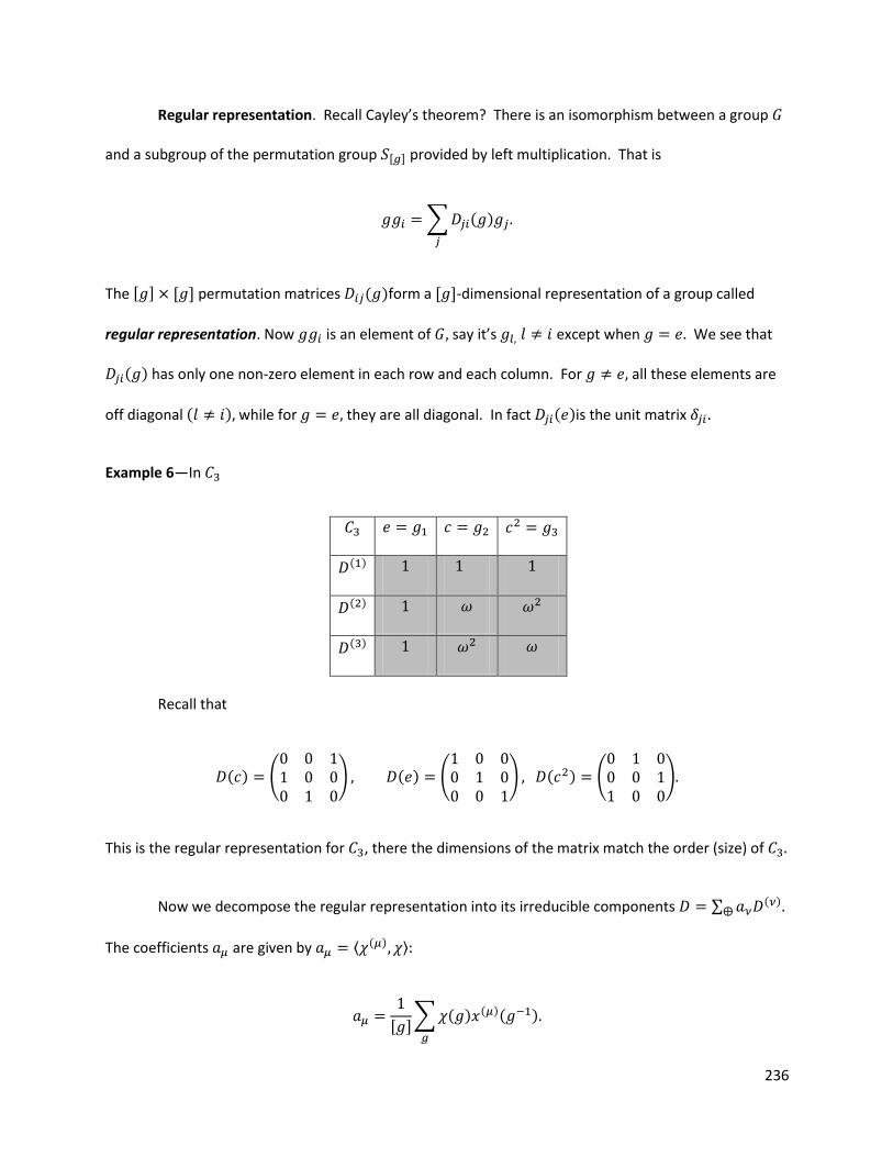
236

Regular representation. Recall Cayley’s theorem? There is an isomorphism between a group

and a subgroup of the permutation group [ ] provided by left multiplication. That is

∑ ( )

The [ ] [ ] permutation matrices ( )form a [ ]-dimensional representation of a group called

regular representation. Now is an element of say it’s except when We see that

( ) has only one non-zero element in each row and each column. For all these elements are

off diagonal ( ) while for they are all diagonal. In fact ( )is the unit matrix

Example 6—In

( )

( )

( )

Recall that

( ) (

) ( ) (

) ( ) (

)

This is the regular representation for , there the dimensions of the matrix match the order (size) of

Now we decompose the regular representation into its irreducible components ∑ ( )

The coefficients are given by ⟨ ( ) ⟩

[ ]∑ ( ) ( )( )

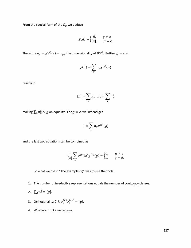
237

From the special form of the we deduce

( ) {

[ ]

Therefore ( )( ) the dimensionality of ( ) Putting in

( ) ∑ ( )( )

results in

[ ] ∑ ∑

making ∑ an equality. For we instead get

∑ ( )( )

and the last two equations can be combined as

[ ]∑ ( )( ) ( )( ) {

So what we did in “The example (5)” was to use the tools:

1. The number of irreducible representations equals the number of conjugacy classes.

2. ∑ [ ]

3. Orthogonality: ∑ ( )

( ) [ ]

4. Whatever tricks we can use.

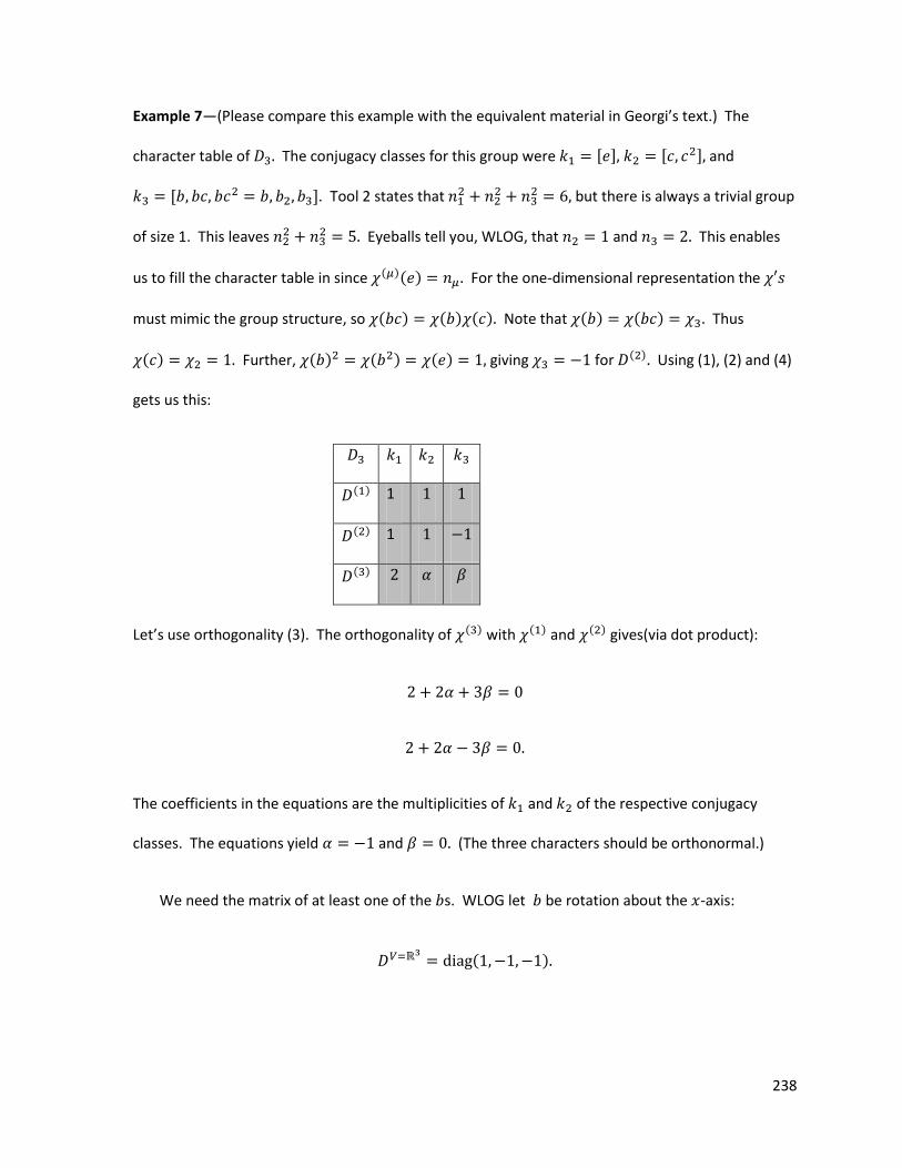
238

Example 7—(Please compare this example with the equivalent material in Georgi’s text.) The

character table of The conjugacy classes for this group were [ ] [ ] and

[ ]. Tool 2 states that

but there is always a trivial group

of size 1. This leaves

Eyeballs tell you, WLOG, that and This enables

us to fill the character table in since ( )( ) For the one-dimensional representation the

must mimic the group structure, so ( ) ( ) ( ) Note that ( ) ( ) Thus

( ) Further, ( ) ( ) ( ) giving for ( ) Using (1), (2) and (4)

gets us this:

( ) 1

( ) 1

( )

Let’s use orthogonality (3). The orthogonality of ( ) with ( ) and ( ) gives(via dot product):

The coefficients in the equations are the multiplicities of and of the respective conjugacy

classes. The equations yield and (The three characters should be orthonormal.)

We need the matrix of at least one of the s. WLOG let be rotation about the -axis:

( )

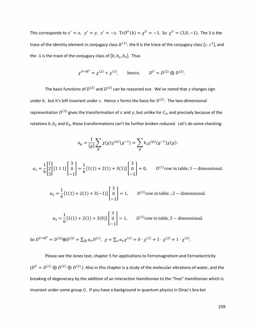
239

This corresponds to ( ) So ( ) The 3 is the

trace of the identity element in conjugacy class ( ), the 0 is the trace of the conjugacy class [ ] and

the -1 is the trace of the conjugacy class of [ ] Thus

( ) ( ) ( ) ( )

The basis functions of ( ) and ( ) can be reasoned out. We’ve noted that changes sign

under but it’s left invariant under Hence forms the basis for ( ) The two-dimensional

representation ( ) gives the transformation of and but unlike for and precisely because of the

rotations and , these transformations can’t be further broken reduced. Let’s do some checking:

[ ]∑ ( ) ( )( )

∑ ( )( ) ( )

[ ] [ ] [

]

[ ( ) ( ) ( )] [

] ( )

[ ( ) ( ) ( )] [

] ( )

[ ( ) ( ) ( )] [

] ( )

So ( ) ( ) ∑

( ) ∑ ( ) ( ) ( ) ( )

Please see the Jones text, chapter 5 for applications to Ferromagnetism and Ferroelectricity

( ( ) ( ) ( ) ) Also in this chapter is a study of the molecular vibrations of water, and the

breaking of degeneracy by the addition of an interaction Hamiltonian to the “free” Hamiltonian which is

invariant under some group If you have a background in quantum physics in Dirac’s bra-ket

240

formalism (there is a quick review in the appendix of Jones) you have sufficient background to

understand the first chapter of Georgi’s text, which contains the identical material BUT in Dirac’s bra-ket

notation, and the definition of projection operators together with a great physical example of the power

of these methods for discrete groups. The remainder of Georgi then tackles continuous (Lie) groups,

this material being paralleled with Jones from chapter 6 to its end. This latter material is what you need

to grasp not only the Standard Model of physics, but its generalizations starting with SU(5) grand

unification theory (the SU(5) GUT). I strongly recommend you read the group theoretic material (in the

appendix as well) of Michio Kaku’s text, “Quantum Field Theory, A Modern Introduction,” Oxford, 1993.

Review and make sure you understand the quantum mechanics of spin and angular momenta, spinors

and tensors at the level of “Quantum Mechanics,” Vols. I and II by C. Cohen-Tannoudji, B. Diu, and F.

Laloë, A Wiley-Interscience Publication, 1977.

Thankfully, only two more algebraic blocks remain in these notes. The first chapter of Gilmore’s

2008 text tying what we’ve just studied to Galois theory follows next. This is proceeded by a few notes I

wrote to make “Lie Algebras in Particle Physics,” by H. Georgi more readable starting with his chapter 2.

I consolidated his sloppy book with the appropriate chapters from the treatment of continuous groups

in Jones (chapter 6-end), and may one day write up these latter notes. For now we turn to Galois

theory. The coverage of this material will be fast paced. Then it’s on to the last notes on group theory

covering the adjoint representation of the Gell-Mann matrices.

Galois theory.

Galois’ theorem: A polynomial over the complex field can be solved iff its Galois group

contains a chain (tower) of subgroups and is abelian.

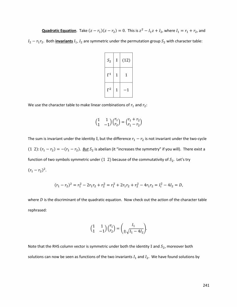
241

Quadratic Equation. Take ( )( ) This is where and

Both invariants , are symmetric under the permutation group with character table:

( )

We use the character table to make linear combinations of and

(

)( ) (

)

The sum is invariant under the identity but the difference is not invariant under the two-cycle

( ) ( ) ( ) But is abelian (it “increases the symmetry” if you will). There exist a

function of two symbols symmetric under ( ) because of the commutativity of Let’s try

( )

( )

where is the discriminant of the quadratic equation. Now check out the action of the character table

rephrased:

(

) ( ) (

√ )

Note that the RHS column vector is symmetric under both the identity and , moreover both

solutions can now be seen as functions of the two invariants and We have found solutions by

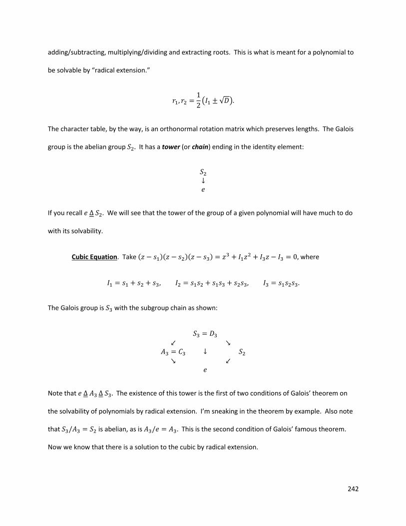
242

adding/subtracting, multiplying/dividing and extracting roots. This is what is meant for a polynomial to

be solvable by “radical extension.”

( √ )

The character table, by the way, is an orthonormal rotation matrix which preserves lengths. The Galois

group is the abelian group It has a tower (or chain) ending in the identity element:

If you recall We will see that the tower of the group of a given polynomial will have much to do

with its solvability.

Cubic Equation. Take ( )( )( ) where

The Galois group is with the subgroup chain as shown:

Note that The existence of this tower is the first of two conditions of Galois’ theorem on

the solvability of polynomials by radical extension. I’m sneaking in the theorem by example. Also note

that is abelian, as is This is the second condition of Galois’ famous theorem.

Now we know that there is a solution to the cubic by radical extension.

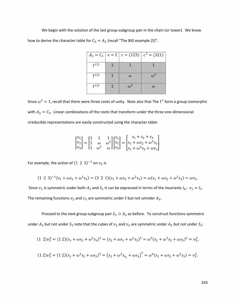
243

We begin with the solution of the last group-subgroup pair in the chain (or tower). We know

how to derive the character table for (recall “The BIG example (5)”:

( ) ( )

( )

( )

( )

Since recall that there were three roots of unity. Note also that The form a group isomorphic

with Linear combinations of the roots that transform under the three one-dimensional

irreducible representations are easily constructed using the character table:

[

] [

] [

] [

]

For example, the action of ( ) on is

( ) ( ) ( )( ) ( )

Since is symmetric under both and it can be expressed in terms of the invariants

The remaining functions and are symmetric under but not umnder

Proceed to the next group-subgroup pair as before. To construct functions symmetric

under but not under note that the cubes of and are symmetric under but not under

( ) ( )( )

( ) ( )

( ) ( )( )

( ) ( )

244

Since permutes the functions and

it is the Galois group of the resolvent quadratic

equation whose two roots are and

This equation has the form:

( )(

)

(We know how to solve quadratic equations.) Take note that and are symmetric under They

can then be expressed in terms of the invariants and of the original cubic equation as follows:

∑

∑

This sum can be greatly simplified by letting To do this, shift the origin with

Then the auxiliary cubic equation has structure

The two invariants

can then be expressed in terms of the invariants

as follows:

245

The resolvent quadratic equation whose solution provides

is ( ) (

)

The two solutions to this resolvent equation are

[(

) ]

The roots

and are obtained by taking the cube roots of and

{

[(

) ]

}

Finally the roots and are linearly related to and by:

[

] [

] [

] [

]

Quartic equation. The general quartic has form

( )( )( )( )

For later convenience we will construct the auxiliary quartic by shifting the origin of coordinates by

(Tschirnhaus transformation). The

( )( )(

)( )

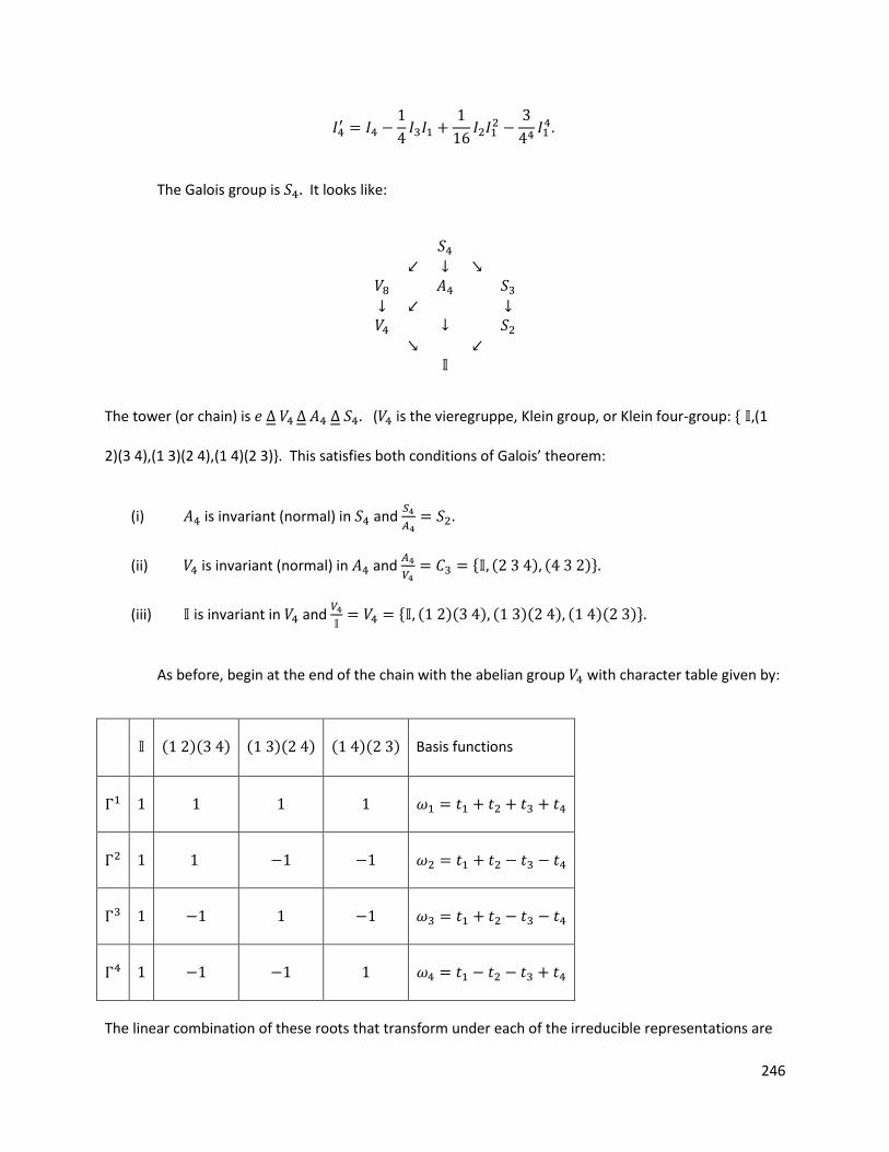
246

The Galois group is It looks like:

The tower (or chain) is ( is the vieregruppe, Klein group, or Klein four-group: { (1

2)(3 4),(1 3)(2 4),(1 4)(2 3)}. This satisfies both conditions of Galois’ theorem:

(i) is invariant (normal) in and

(ii) is invariant (normal) in and

{ ( ) ( )}

(iii) is invariant in and

{ ( )( ) ( )( ) ( )( )}

As before, begin at the end of the chain with the abelian group with character table given by:

( )( ) ( )( ) ( )( ) Basis functions

The linear combination of these roots that transform under each of the irreducible representations are

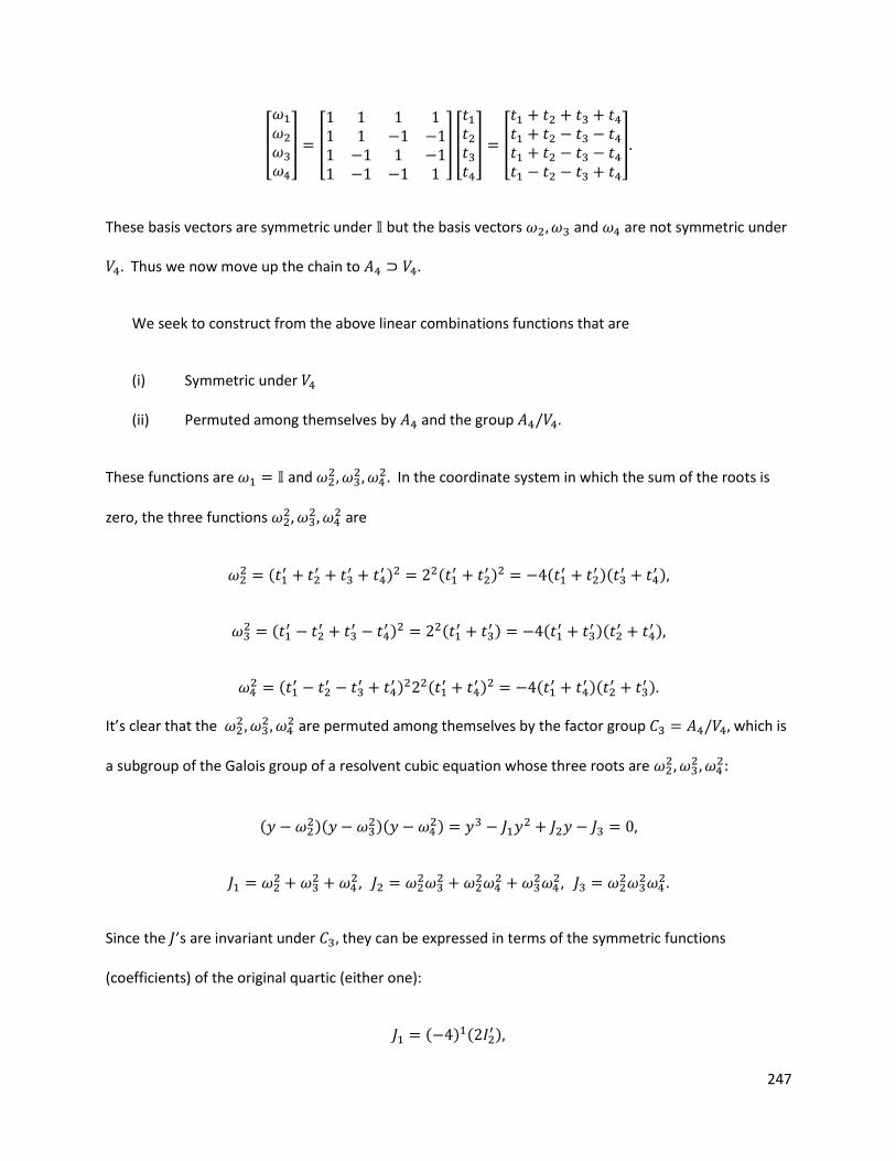
247

[

] [

] [

] [

]

These basis vectors are symmetric under but the basis vectors and are not symmetric under

Thus we now move up the chain to

We seek to construct from the above linear combinations functions that are

(i) Symmetric under

(ii) Permuted among themselves by and the group

These functions are and

In the coordinate system in which the sum of the roots is

zero, the three functions

are

(

) (

) (

)(

)

(

) (

) (

)(

)

(

) (

) (

)(

)

It’s clear that the

are permuted among themselves by the factor group which is

a subgroup of the Galois group of a resolvent cubic equation whose three roots are

( )(

)( )

Since the ’s are invariant under they can be expressed in terms of the symmetric functions

(coefficients) of the original quartic (either one):

( ) ( )

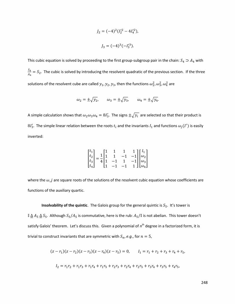
248

( ) (

)

( ) ( )

This cubic equation is solved by proceeding to the first group-subgroup pair in the chain: with

The cubic is solved by introducing the resolvent quadratic of the previous section. If the three

solutions of the resolvent cube are called then the functions

are

√ √ √

A simple calculation shows that The signs √ are selected so that their product is

The simple linear relation between the roots and the invariants and functions (

) is easily

inverted:

[

]

[

] [

]

where the are square roots of the solutions of the resolvent cubic equation whose coefficients are

functions of the auxiliary quartic.

Insolvability of the quintic. The Galois group for the general quintic is It’s tower is

Although is commutative, here is the rub: is not abelian. This tower doesn’t

satisfy Galois’ theorem. Let’s discuss this. Given a polynomial of nth degree in a factorized form, it is

trivial to construct invariants that are symmetric with e.g., for

( )( )( )( )( )

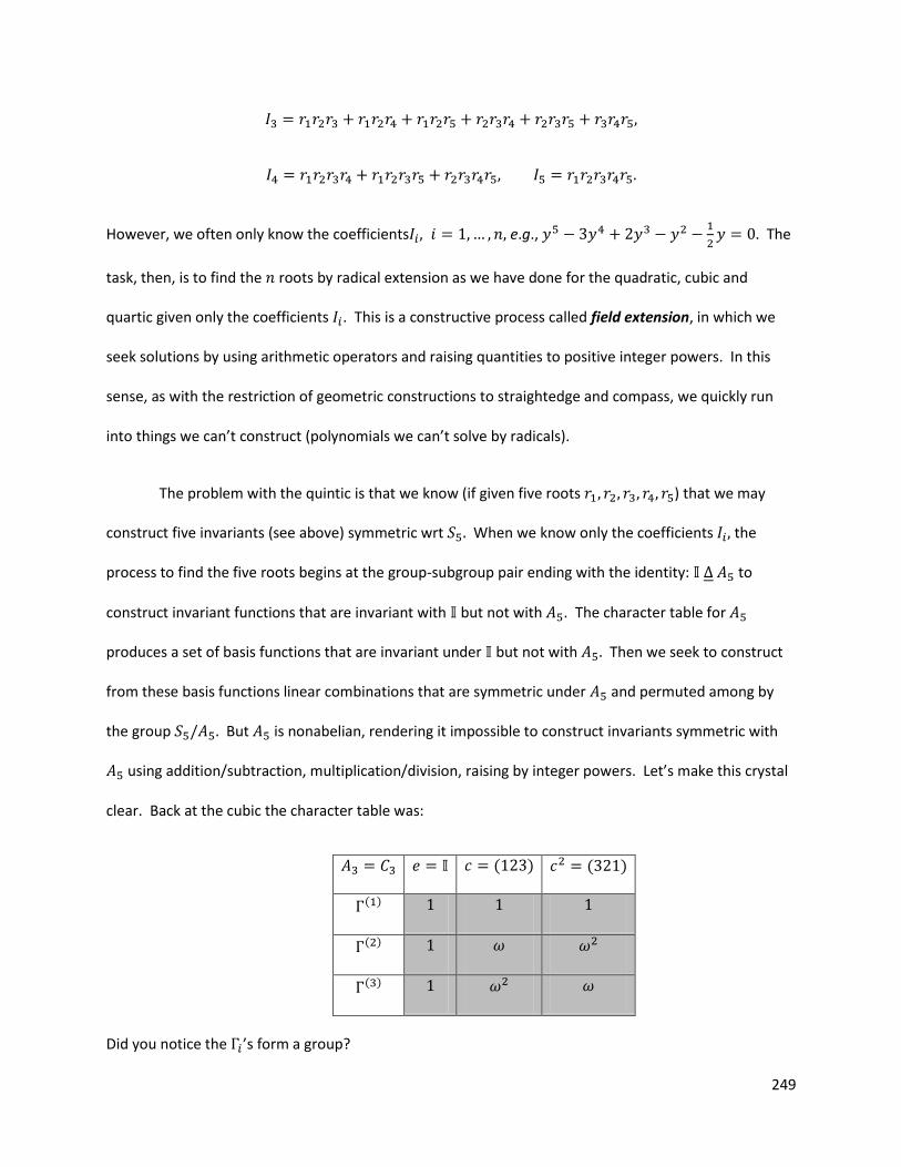
249

However, we often only know the coefficients e.g.,

The

task, then, is to find the roots by radical extension as we have done for the quadratic, cubic and

quartic given only the coefficients . This is a constructive process called field extension, in which we

seek solutions by using arithmetic operators and raising quantities to positive integer powers. In this

sense, as with the restriction of geometric constructions to straightedge and compass, we quickly run

into things we can’t construct (polynomials we can’t solve by radicals).

The problem with the quintic is that we know (if given five roots ) that we may

construct five invariants (see above) symmetric wrt When we know only the coefficients the

process to find the five roots begins at the group-subgroup pair ending with the identity: to

construct invariant functions that are invariant with but not with . The character table for

produces a set of basis functions that are invariant under but not with Then we seek to construct

from these basis functions linear combinations that are symmetric under and permuted among by

the group But is nonabelian, rendering it impossible to construct invariants symmetric with

using addition/subtraction, multiplication/division, raising by integer powers. Let’s make this crystal

clear. Back at the cubic the character table was:

( ) ( )

( )

( )

( )

Did you notice the ’s form a group?

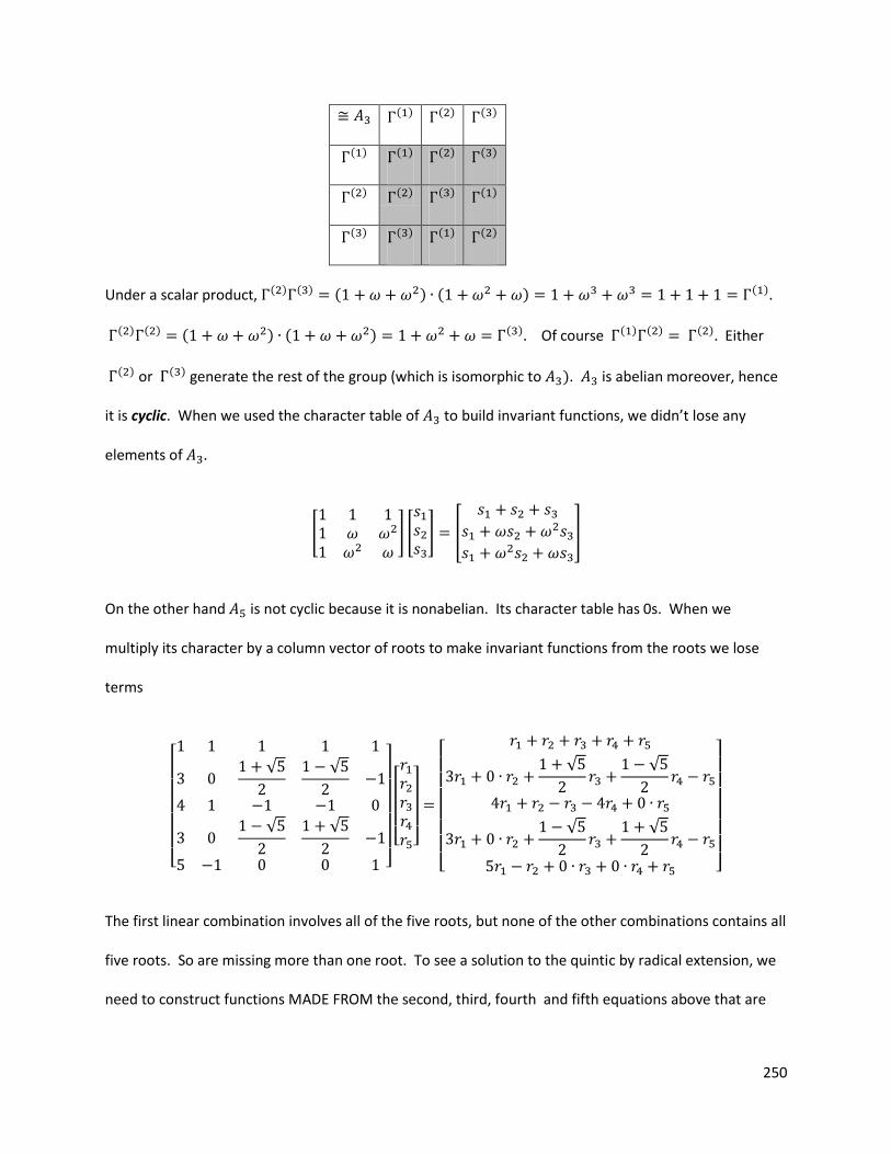
250

( ) ( ) ( )

( ) ( ) ( ) ( )

( ) ( ) ( ) ( )

( ) ( ) ( ) ( )

Under a scalar product, ( ) ( ) ( ) ( ) ( )

( ) ( ) ( ) ( ) ( ) Of course ( ) ( ) ( ) Either

( ) or ( ) generate the rest of the group (which is isomorphic to ). is abelian moreover, hence

it is cyclic. When we used the character table of to build invariant functions, we didn’t lose any

elements of

[

] [

] [

]

On the other hand is not cyclic because it is nonabelian. Its character table has 0s. When we

multiply its character by a column vector of roots to make invariant functions from the roots we lose

terms

[

√

√

√

√

]

[ ]

[

√

√

√

√

]

The first linear combination involves all of the five roots, but none of the other combinations contains all

five roots. So are missing more than one root. To see a solution to the quintic by radical extension, we

need to construct functions MADE FROM the second, third, fourth and fifth equations above that are

251

invariant under the interchange of symbols. Impossible. Hence the quintic is unsolvable by radical

extension.

Be water my friend. “One step beyond the solvable equation,” Sander Bessels, PhD dissertation

2006, uses Galois theory, Klein’s icosahedron and elliptic curves to solve the general quintic. To the

symmetries of the Standard Model, physicists have added supersymmetry (SUSY). Many infinites have

died. Let’s proceed to the last of the algebraic blocks. After dealing with discrete groups, Jones

proceeds to continuous groups. These notes provide several step-by-step examples that detail the

theory developed in Jones and, supposedly, in H. Georgi’s book on Lie algebras in particle physics from

Isospin to unified theories.

Self-contained algebra prerequisites for the Standard Model, GUTs and TOEs. We will study

SU(2) and SU(3) in detail via tensor product and direct sum matrix mathematics, ladder operators and

Young’s tableaux. This is where your background in junior or senior level exposure to quantum

mechanical addition of angular momentum will come in handy. It is your option whether you read the

material on the Wigner-Eckart theorem, which is useful for computing selection rules. What we learn

from SU(2) and SU(3) will then be generalized to study the Cartan subalgebra, the attendant ladder

operators, the Killing form, root and weight diagrams and Dynkin diagrams. These are the tools to

“play” group theory with theories beyond the Standard Model, e.g., SU(5) or Lissi’s TOE.

Basics [Highly augmented with my notes the following material is excerpted from “Spin and the

addition of angular momentum using tensor notation,” Joel C. Corbo, 2007]. The aim of this section is to

see the explicit connection between the coupled and uncoupled basis (between tensor products and

direct sums that is). The spin operators and have commutation relations given by

[ ] [ ] [ ]

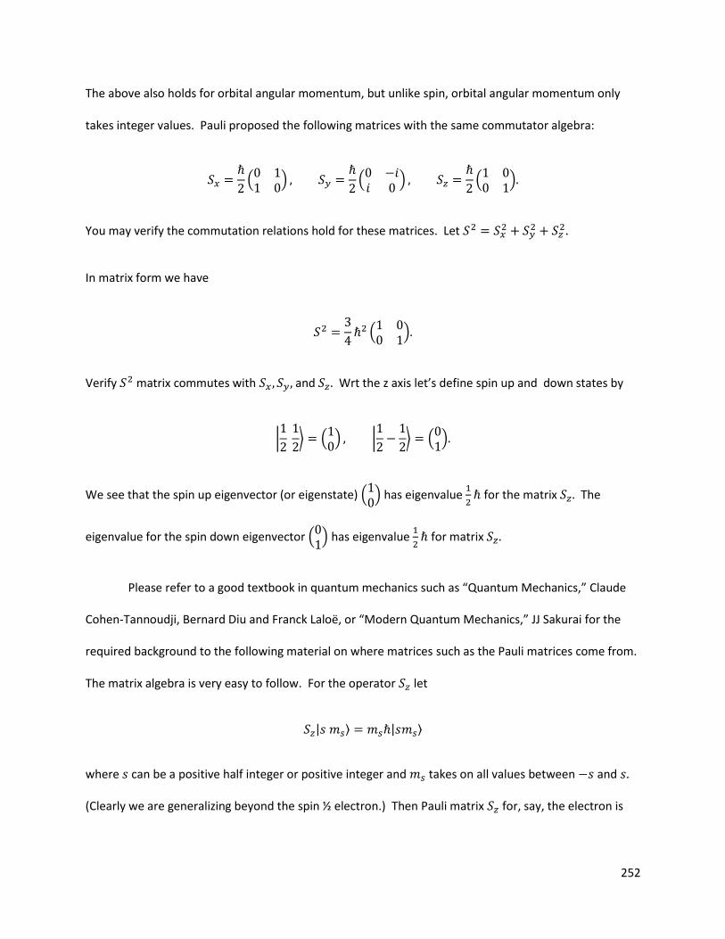
252

The above also holds for orbital angular momentum, but unlike spin, orbital angular momentum only

takes integer values. Pauli proposed the following matrices with the same commutator algebra:

(

)

(

)

(

)

You may verify the commutation relations hold for these matrices. Let

In matrix form we have

(

)

Verify matrix commutes with and Wrt the z axis let’s define spin up and down states by

|

⟩ (

) |

⟩ (

)

We see that the spin up eigenvector (or eigenstate) ( ) has eigenvalue

for the matrix The

eigenvalue for the spin down eigenvector ( ) has eigenvalue

for matrix

Please refer to a good textbook in quantum mechanics such as “Quantum Mechanics,” Claude

Cohen-Tannoudji, Bernard Diu and Franck Laloë, or “Modern Quantum Mechanics,” JJ Sakurai for the

required background to the following material on where matrices such as the Pauli matrices come from.

The matrix algebra is very easy to follow. For the operator let

| ⟩ | ⟩

where can be a positive half integer or positive integer and takes on all values between and

(Clearly we are generalizing beyond the spin ½ electron.) Then Pauli matrix for, say, the electron is

253

(⟨

| |

⟩ ⟨

| |

⟩

⟨

| |

⟩ ⟨

| |

⟩

) (

⟨

|

⟩

⟨

|

⟩

⟨

|

⟩

⟨

|

⟩

)

(

)

If it happened that the particle in question was a spin one particle, then the matrix would be

(

⟨ | | ⟩ ⟨ | | ⟩ ⟨ | | ⟩

⟨ | | ⟩ ⟨ | | ⟩ ⟨ | | ⟩

⟨ | | ⟩ ⟨ | | ⟩ ⟨ | | ⟩)

(

)

Let me introduce two new operators and corresponding matrices built from linear combinations of

and . Let By inversion,

( ) and

( ) Check it out. Add

to to get

For we have

| ⟩ √ ( ) ( )| ⟩

For an electron let’s compute the matrix for

(⟨

| |

⟩ ⟨

| |

⟩

⟨

| |

⟩ ⟨

| |

⟩

) (

)

This jives with summing the matrices for and . Lastly for we have

| ⟩ ( )| ⟩

Let’s proceed to describing systems with more than one particle. First let’s restrict ourselves to

two particles, one with spin and another with spin It turns out, as you shall see, that there are two

bases for describing the possible spin states these two particles can be in. Let’s consider the so-called

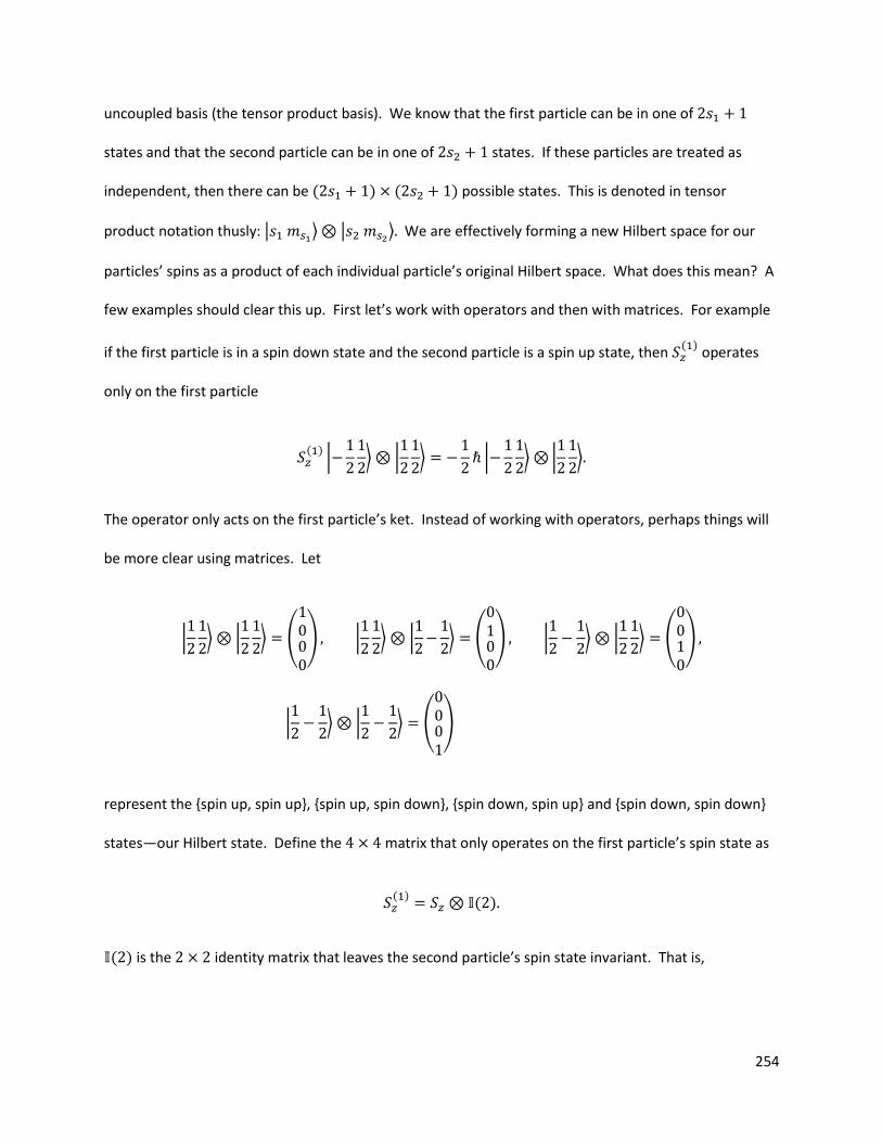
254

uncoupled basis (the tensor product basis). We know that the first particle can be in one of

states and that the second particle can be in one of states. If these particles are treated as

independent, then there can be ( ) ( ) possible states. This is denoted in tensor

product notation thusly: | ⟩ | ⟩ We are effectively forming a new Hilbert space for our

particles’ spins as a product of each individual particle’s original Hilbert space. What does this mean? A

few examples should clear this up. First let’s work with operators and then with matrices. For example

if the first particle is in a spin down state and the second particle is a spin up state, then ( )

operates

only on the first particle

( )

|

⟩ |

⟩

|

⟩ |

⟩

The operator only acts on the first particle’s ket. Instead of working with operators, perhaps things will

be more clear using matrices. Let

|

⟩ |

⟩ (

) |

⟩ |

⟩ (

) |

⟩ |

⟩ (

)

|

⟩ |

⟩ (

)

represent the {spin up, spin up}, {spin up, spin down}, {spin down, spin up} and {spin down, spin down}

states—our Hilbert state. Define the matrix that only operates on the first particle’s spin state as

( ) ( )

( ) is the identity matrix that leaves the second particle’s spin state invariant. That is,

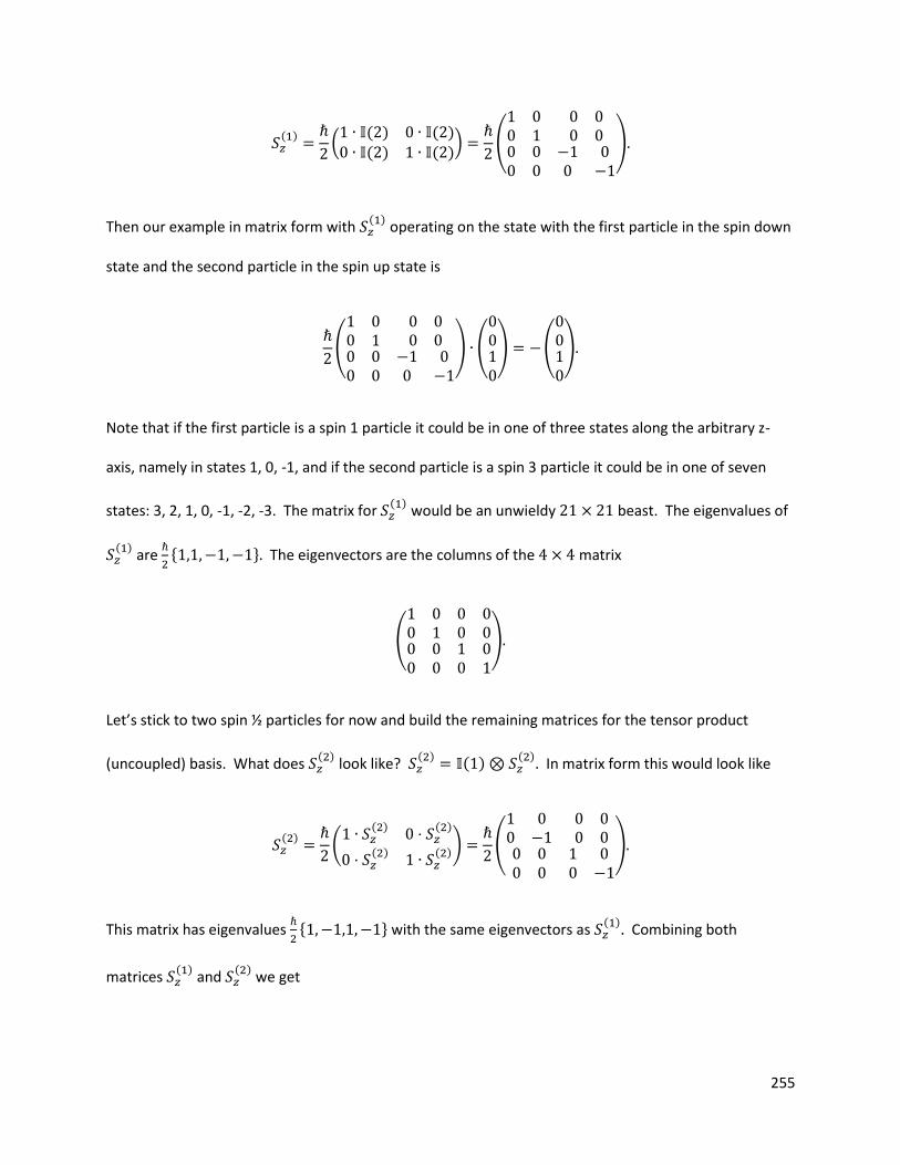
255

( )

( ( ) ( ) ( ) ( )

)

(

)

Then our example in matrix form with ( )

operating on the state with the first particle in the spin down

state and the second particle in the spin up state is

(

) (

) (

)

Note that if the first particle is a spin 1 particle it could be in one of three states along the arbitrary z-

axis, namely in states 1, 0, -1, and if the second particle is a spin 3 particle it could be in one of seven

states: 3, 2, 1, 0, -1, -2, -3. The matrix for ( ) would be an unwieldy beast. The eigenvalues of

( ) are

{ } The eigenvectors are the columns of the matrix

(

)

Let’s stick to two spin ½ particles for now and build the remaining matrices for the tensor product

(uncoupled) basis. What does ( ) look like?

( ) ( ) ( ) In matrix form this would look like

( )

(

( ) ( )

( )

( ))

(

)

This matrix has eigenvalues

{ } with the same eigenvectors as

( ) Combining both

matrices ( ) and

( ) we get

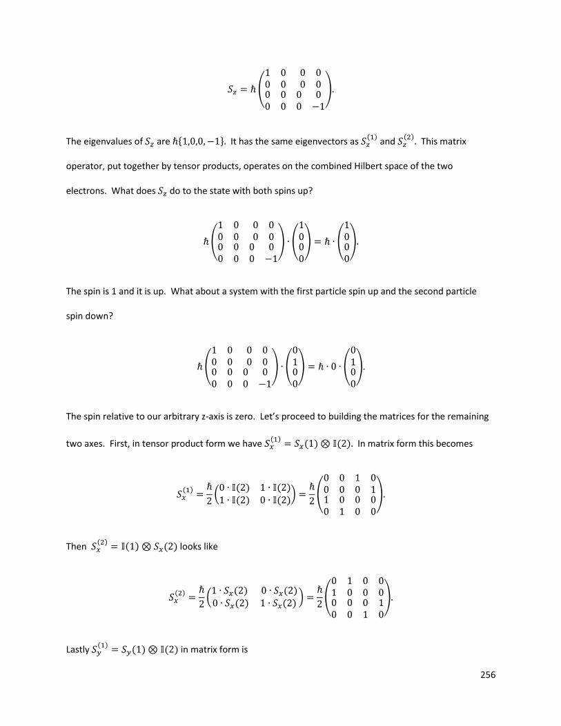
256

(

)

The eigenvalues of are { } It has the same eigenvectors as ( )

and ( )

This matrix

operator, put together by tensor products, operates on the combined Hilbert space of the two

electrons. What does do to the state with both spins up?

(

) (

) (

)

The spin is 1 and it is up. What about a system with the first particle spin up and the second particle

spin down?

(

) (

) (

)

The spin relative to our arbitrary z-axis is zero. Let’s proceed to building the matrices for the remaining

two axes. First, in tensor product form we have ( )

( ) ( ) In matrix form this becomes

( )

( ( ) ( ) ( ) ( )

)

(

)

Then ( ) ( ) ( ) looks like

( )

( ( ) ( ) ( ) ( )

)

(

)

Lastly ( ) ( ) ( ) in matrix form is

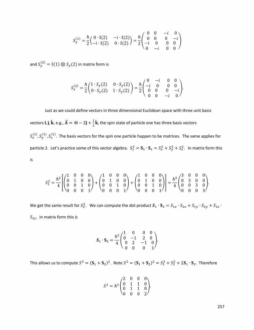
257

( )

( ( ) ( ) ( ) ( )

)

(

)

and ( )

( ) ( ) in matrix form is

( )

( ( ) ( )

( ) ( ) )

(

)

Just as we could define vectors in three dimensional Euclidean space with three unit basis

vectors , e.g.,

the spin state of particle one has three basis vectors

( )

( )

( )

The basis vectors for the spin one particle happen to be matrices. The same applies for

particle 2. Let’s practice some of this vector algebra.

In matrix form this

is

[(

) (

) (

)]

(

)

We get the same result for We can compute the dot product

. In matrix form this is

(

)

This allows us to compute ( ) . Note ( )

Therefore

(

)

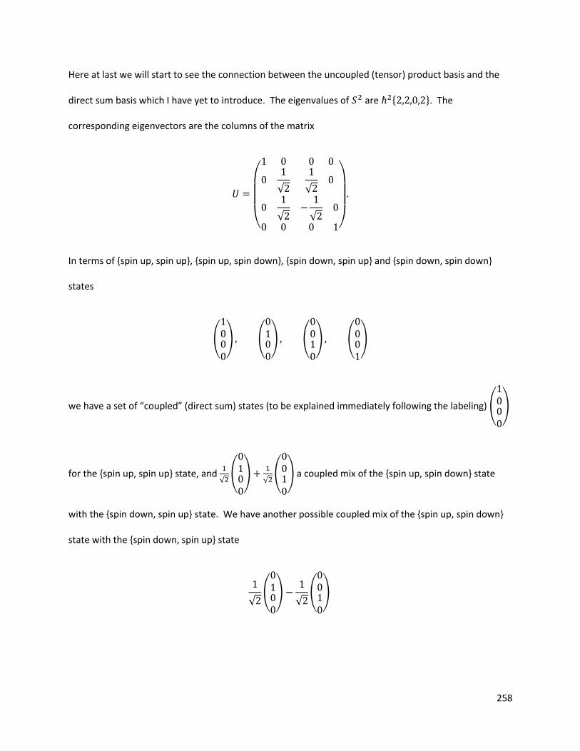
258

Here at last we will start to see the connection between the uncoupled (tensor) product basis and the

direct sum basis which I have yet to introduce. The eigenvalues of are { }. The

corresponding eigenvectors are the columns of the matrix

(

√

√

√

√

)

In terms of {spin up, spin up}, {spin up, spin down}, {spin down, spin up} and {spin down, spin down}

states

(

) (

) (

) (

)

we have a set of “coupled” (direct sum) states (to be explained immediately following the labeling) (

)

for the {spin up, spin up} state, and

√ (

)

√ (

) a coupled mix of the {spin up, spin down} state

with the {spin down, spin up} state. We have another possible coupled mix of the {spin up, spin down}

state with the {spin down, spin up} state

√ (

)

√ (

)

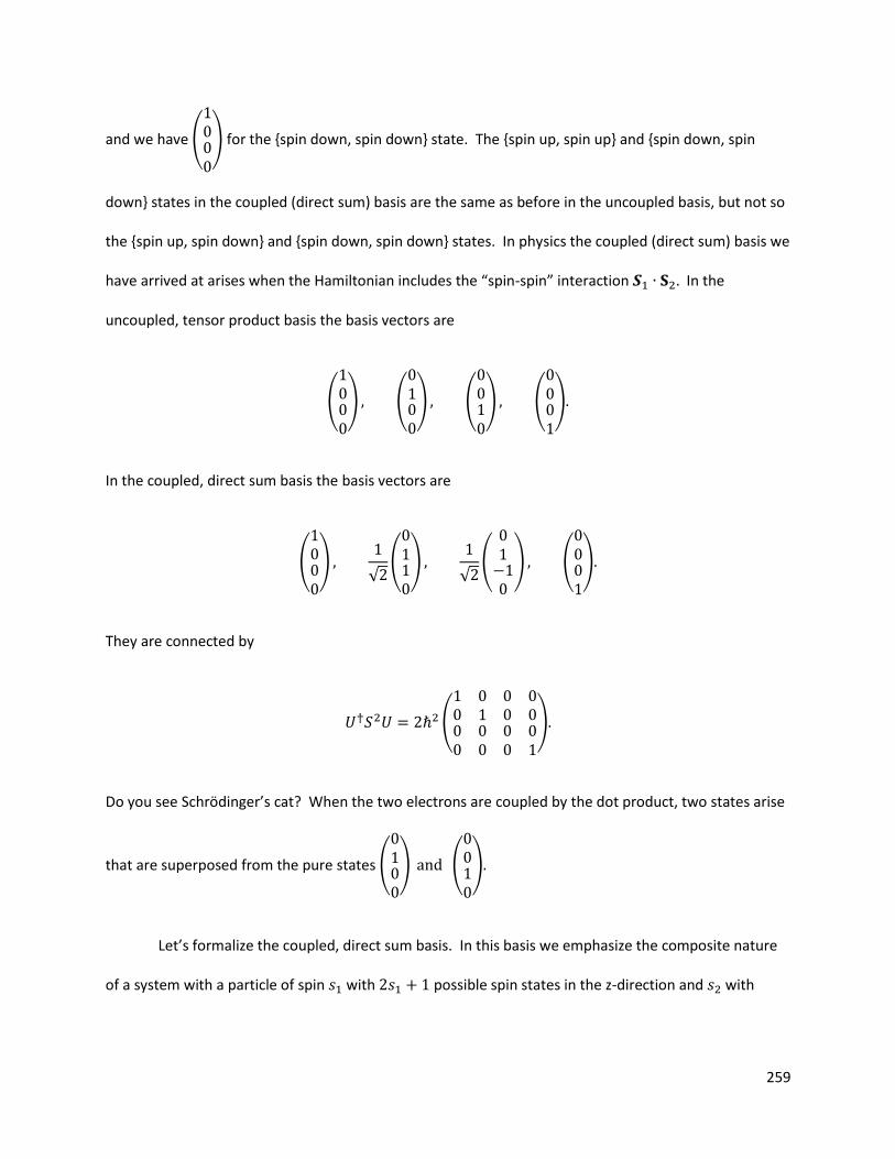
259

and we have (

) for the {spin down, spin down} state. The {spin up, spin up} and {spin down, spin

down} states in the coupled (direct sum) basis are the same as before in the uncoupled basis, but not so

the {spin up, spin down} and {spin down, spin down} states. In physics the coupled (direct sum) basis we

have arrived at arises when the Hamiltonian includes the “spin-spin” interaction In the

uncoupled, tensor product basis the basis vectors are

(

) (

) (

) (

)

In the coupled, direct sum basis the basis vectors are

(

)

√ (

)

√ (

) (

)

They are connected by

(

)

Do you see Schrödinger’s cat? When the two electrons are coupled by the dot product, two states arise

that are superposed from the pure states (

) (

)

Let’s formalize the coupled, direct sum basis. In this basis we emphasize the composite nature

of a system with a particle of spin with possible spin states in the z-direction and with

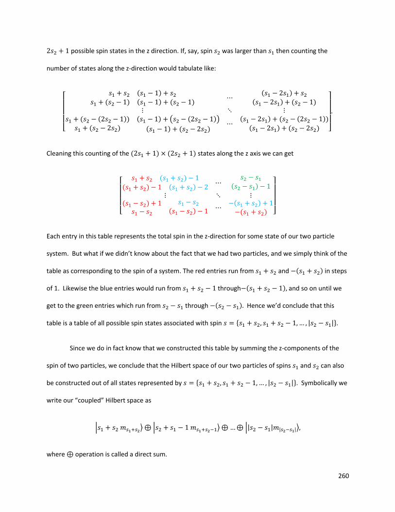
260

possible spin states in the z direction. If, say, spin was larger than then counting the

number of states along the z-direction would tabulate like:

[

( ) ( ) ( ) ( )

( )

( ) ( )

( ( )) ( )

( ) ( ( ))

( ) ( )

( ) ( ( ))( ) ( ) ]

Cleaning this counting of the ( ) ( ) states along the z axis we can get

[

( )

( ) ( )

( )

( )

( )

( ) ( ) ]

Each entry in this table represents the total spin in the z-direction for some state of our two particle

system. But what if we didn’t know about the fact that we had two particles, and we simply think of the

table as corresponding to the spin of a system. The red entries run from and ( ) in steps

of 1. Likewise the blue entries would run from through ( ) and so on until we

get to the green entries which run from through ( ) Hence we’d conclude that this

table is a table of all possible spin states associated with spin { | |}.

Since we do in fact know that we constructed this table by summing the z-components of the

spin of two particles, we conclude that the Hilbert space of our two particles of spins and can also

be constructed out of all states represented by { | |}. Symbolically we

write our “coupled” Hilbert space as

| ⟩ | ⟩ || | | |⟩

where operation is called a direct sum.

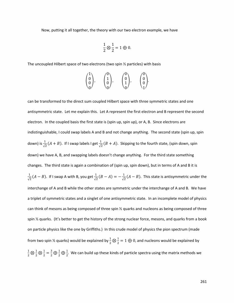
261

Now, putting it all together, the theory with our two electron example, we have

The uncoupled Hilbert space of two electrons (two spin ½ particles) with basis

(

) (

) (

) (

)

can be transformed to the direct sum coupled Hilbert space with three symmetric states and one

antisymmetric state. Let me explain this. Let A represent the first electron and B represent the second

electron. In the coupled basis the first state is (spin up, spin up), or A, B. Since electrons are

indistinguishable, I could swap labels A and B and not change anything. The second state (spin up, spin

down) is

√ ( ) If I swap labels I get

√ ( ). Skipping to the fourth state, (spin down, spin

down) we have A, B, and swapping labels doesn’t change anything. For the third state something

changes. The third state is again a combination of (spin up, spin down), but in terms of A and B it is

√ ( ) If I swap A with B, you get

√ ( )

√ ( ) This state is antisymmetric under the

interchange of A and B while the other states are symmetric under the interchange of A and B. We have

a triplet of symmetric states and a singlet of one antisymmetric state. In an incomplete model of physics

can think of mesons as being composed of three spin ½ quarks and nucleons as being composed of three

spin ½ quarks. (It’s better to get the history of the strong nuclear force, mesons, and quarks from a book

on particle physics like the one by Griffiths.) In this crude model of physics the pion spectrum (made

from two spin ½ quarks) would be explained by

and nucleons would be explained by

We can build up these kinds of particle spectra using the matrix methods we

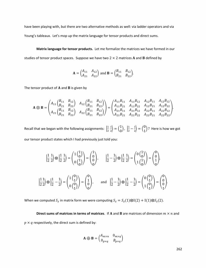
262

have been playing with, but there are two alternative methods as well: via ladder operators and via

Young’s tableaux. Let’s mop up the matrix language for tensor products and direct sums.

Matrix language for tensor products. Let me formalize the matrices we have formed in our

studies of tensor product spaces. Suppose we have two matrices and defined by

(

) (

)

The tensor product of and is given by

( (

) (

)

(

) (

)) (

)

Recall that we began with the following assignments: |

⟩ (

) |

⟩ (

) Here is how we got

our tensor product states which I had previously just told you:

|

⟩ |

⟩ (

( )

( )) (

) |

⟩ |

⟩ (

( )

( )) (

)

|

⟩ |

⟩ (

( )

( )) (

) |

⟩ |

⟩ (

( )

( )) (

)

When we computed in matrix form we were computing ( ) ( ) ( ) ( ).

Direct sums of matrices in terms of matrices. If and are matrices of dimension and

respectively, the direct sum is defined by:

(

)

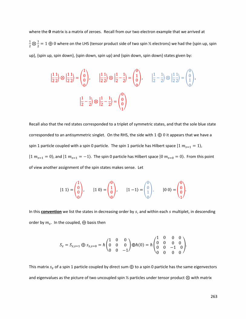
263

where the matrix is a matrix of zeroes. Recall from our two electron example that we arrived at

where on the LHS (tensor product side of two spin ½ electrons) we had the {spin up, spin

up}, {spin up, spin down}, {spin down, spin up} and {spin down, spin down} states given by:

|

⟩ |

⟩ (

) |

⟩ |

⟩ (

) |

⟩ |

⟩ (

)

|

⟩ |

⟩ (

)

Recall also that the red states corresponded to a triplet of symmetric states, and that the sole blue state

corresponded to an antisymmetric singlet. On the RHS, the side with it appears that we have a

spin 1 particle coupled with a spin 0 particle. The spin 1 particle has Hilbert space | ⟩

| ⟩ and | ⟩ The spin 0 particle has Hilbert space | ⟩ From this point

of view another assignment of the spin states makes sense. Let

| ⟩ (

) | ⟩ (

) | ⟩ (

) | ⟩ (

)

In this convention we list the states in decreasing order by , and within each multiplet, in descending

order by . In the coupled, basis then

(

) ( ) (

)

This matrix of a spin 1 particle coupled by direct sum to a spin 0 particle has the same eigenvectors

and eigenvalues as the picture of two uncoupled spin ½ particles under tensor product with matrix

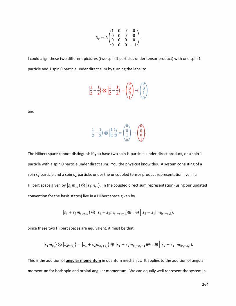
264

(

)

I could align these two different pictures (two spin ½ particles under tensor product) with one spin 1

particle and 1 spin 0 particle under direct sum by turning the label to

|

⟩ |

⟩ (

) (

)

and

|

⟩ |

⟩ (

) (

)

The Hilbert space cannot distinguish if you have two spin ½ particles under direct product, or a spin 1

particle with a spin 0 particle under direct sum. You the physicist know this. A system consisting of a

spin particle and a spin particle, under the uncoupled tensor product representation live in a

Hilbert space given by | ⟩ | ⟩. In the coupled direct sum representation (using our updated

convention for the basis states) live in a Hilbert space given by

| ⟩ | ⟩ || | | |⟩

Since these two Hilbert spaces are equivalent, it must be that

| ⟩ | ⟩ | ⟩ | ⟩ || | | |⟩

This is the addition of angular momentum in quantum mechanics. It applies to the addition of angular

momentum for both spin and orbital angular momentum. We can equally well represent the system in

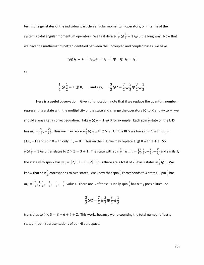
265

terms of eigenstates of the individual particle’s angular momentum operators, or in terms of the

system’s total angular momentum operators. We first derived

the long way. Now that

we have the mathematics better identified between the uncoupled and coupled bases, we have

| |

so

Here is a useful observation. Given this notation, note that if we replace the quantum number

representing a state with the multiplicity of the state and change the operators to and to , we

should always get a correct equation. Take

for example. Each spin

state on the LHS

has {

} Thus we may replace

with . On the RHS we have spin 1 with

{ } and spin 0 with only Thus on the RHS we may replace with So

translates to The state with spin

has {

} and similarly

the state with spin 2 has { }. Thus there are a total of 20 basis states in

. We

know that spin

corresponds to two states. We know that spin

corresponds to 4 states. Spin

has

{

} values. There are 6 of these. Finally spin

has 8 possibilities. So

translates to This works because we’re counting the total number of basis

states in both representations of our Hilbert space.

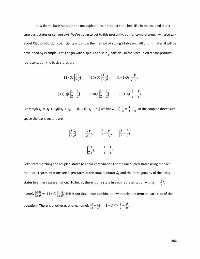
266

How do the basis states in the uncoupled tensor product state look like in the coupled direct

sum basis states or conversely? We’re going to get to this presently, but for completeness I will also talk

about Clebsch-Gordon coefficients and show the method of Young’s tableaux. All of this material will be

developed by example. Let’s begin with a spin 1 and spin

particle. In the uncoupled tensor product

representation the basis states are

| ⟩ |

⟩ | ⟩ |

⟩ | ⟩ |

⟩

| ⟩ |

⟩ | ⟩ |

⟩ | ⟩ |

⟩

From | | we know

. In the coupled direct sum

space the basis vectors are

|

⟩ |

⟩ |

⟩ |

⟩

|

⟩ |

⟩

Let’s start matching the coupled states to linear combinations of the uncoupled states using the fact

that both representations are eigenstates of the total operator and the orthogonality of the basis

states in either representation. To begin, there is one state in each representation with

,

namely |

⟩ | ⟩ |

⟩ This is our first linear combination with only one term on each side of the

equation. There is another easy one, namely |

⟩ | ⟩ |

⟩

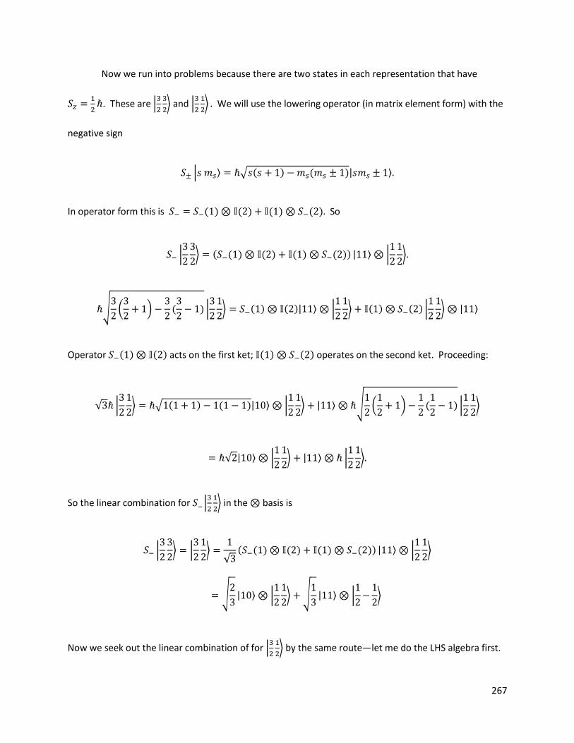
267

Now we run into problems because there are two states in each representation that have

. These are |

⟩ and |

⟩ We will use the lowering operator (in matrix element form) with the

negative sign

| ⟩ √ ( ) ( )| ⟩

In operator form this is ( ) ( ) ( ) ( ) So

|

⟩ ( ( ) ( ) ( ) ( )) | ⟩ |

⟩

√

(

)

(

) |

⟩ ( ) ( )| ⟩ |

⟩ ( ) ( ) |

⟩ | ⟩

Operator ( ) ( ) acts on the first ket; ( ) ( ) operates on the second ket. Proceeding:

√ |

⟩ √ ( ) ( )| ⟩ |

⟩ | ⟩ √

(

)

(

) |

⟩

√ | ⟩ |

⟩ | ⟩ |

⟩

So the linear combination for |

⟩ in the basis is

|

⟩ |

⟩

√ ( ( ) ( ) ( ) ( )) | ⟩ |

⟩

√

| ⟩ |

⟩ √

| ⟩ |

⟩

Now we seek out the linear combination of for |

⟩ by the same route—let me do the LHS algebra first.

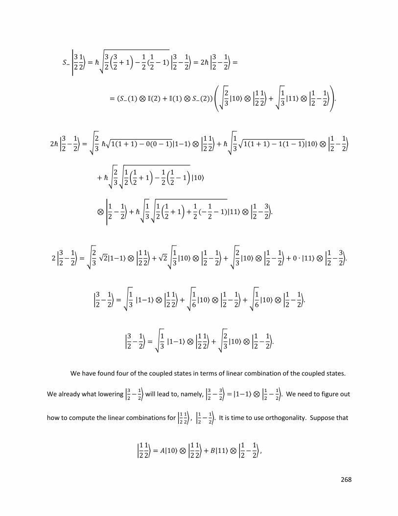
268

|

⟩ √

(

)

(

) |

⟩ |

⟩

( ( ) ( ) ( ) ( ))(√

| ⟩ |

⟩ √

| ⟩ |

⟩)

|

⟩ √

√ ( ) ( )| ⟩ |

⟩ √

√ ( ) ( )| ⟩ |

⟩

√

√

(

)

(

) | ⟩

|

⟩ √

√

(

)

(

)| ⟩ |

⟩

|

⟩ √

√ | ⟩ |

⟩ √ √

| ⟩ |

⟩ √

| ⟩ |

⟩ | ⟩ |

⟩

|

⟩ √

| ⟩ |

⟩ √

| ⟩ |

⟩ √

| ⟩ |

⟩

|

⟩ √

| ⟩ |

⟩ √

| ⟩ |

⟩

We have found four of the coupled states in terms of linear combination of the coupled states.

We already what lowering |

⟩ will lead to, namely, |

⟩ | ⟩ |

⟩ We need to figure out

how to compute the linear combinations for |

⟩ |

⟩ It is time to use orthogonality. Suppose that

|

⟩ | ⟩ |

⟩ | ⟩ |

⟩

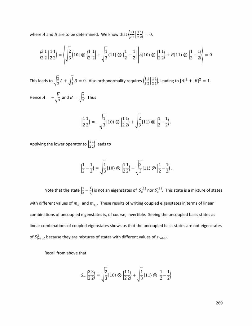
269

where and are to be determined. We know that ⟨

|

⟩

⟨

|

⟩ ⟨√

⟨ | ⟨

| √

⟨ | ⟨

| | | ⟩ |

⟩ | ⟩ |

⟩⟩

This leads to √

√

Also orthonormality requires ⟨

|

⟩, leading to | | | |

Hence √

and √

. Thus

|

⟩ √

| ⟩ |

⟩ √

| ⟩ |

⟩

Applying the lower operator to |

⟩ leads to

|

⟩ √

| ⟩ |

⟩ √

| ⟩ |

⟩

Note that the state |

⟩ is not an eigenstates of

( ) nor

( ). This state is a mixture of states

with different values of and . These results of writing coupled eigenstates in terms of linear

combinations of uncoupled eigenstates is, of course, invertible. Seeing the uncoupled basis states as

linear combinations of coupled eigenstates shows us that the uncoupled basis states are not eigenstates

of because they are mixtures of states with different values of

Recall from above that

|

⟩ √

| ⟩ |

⟩ √

| ⟩ |

⟩

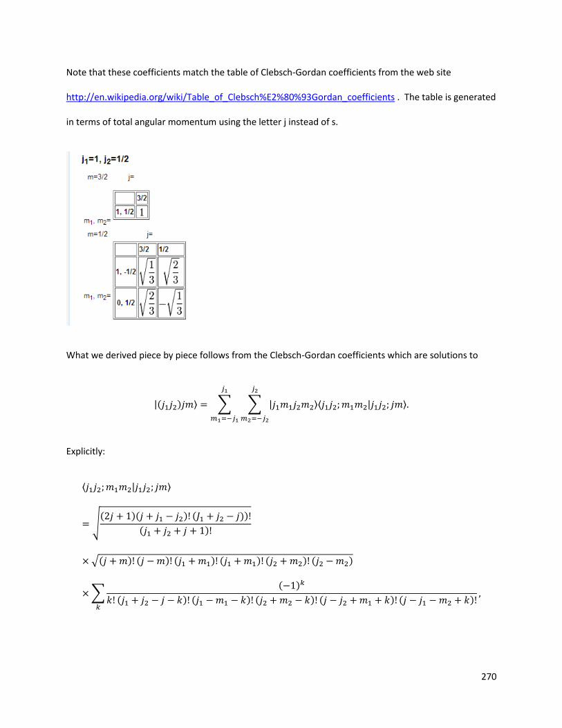
270

Note that these coefficients match the table of Clebsch-Gordan coefficients from the web site

http://en.wikipedia.org/wiki/Table_of_Clebsch%E2%80%93Gordan_coefficients . The table is generated

in terms of total angular momentum using the letter j instead of s.

What we derived piece by piece follows from the Clebsch-Gordan coefficients which are solutions to

|( ) ⟩ ∑ ∑ | ⟩⟨ | ⟩

Explicitly:

⟨ | ⟩

√( )( ) ( ))

( )

√( ) ( ) ( ) ( ) ( ) ( )

∑( )

( ) ( ) ( ) ( ) ( )

271

where the summation is extended over all integer for which the argument above every factorial is

nonnegative. For brevity, solutions with and are omitted. They may be calculated using

the relations

⟨ | ⟩ ( ) ⟨ | ⟩

⟨ | ⟩ ( ) ⟨ | ⟩

Let’s pause to reflect a little about what we have been doing in terms of atoms with many

electrons and in terms of quarks being constituent particles. The mathematics we have been enjoying

so far have dealt with two spin ½ particles. We have learned that there is a triplet state of symmetric

wave functions and a singlet state of antisymmetric wave functions. In historical nuclear physics the

first two quarks were the up and down quark, and their antiparticles. The pions could then be described

as members of an Isospin triplet: the as follows

| ⟩ |

⟩ |

⟩

| ⟩

√ (|

⟩ |

⟩ |

⟩ |

⟩ )

| ⟩ |

⟩ |

⟩

For the details in terms of quarks and antiquarks, please refer to chapter 12 by Melih Sener and Klaus

Schulten in the PDF file at http://www.ks.uiuc.edu/Services/Class/PHYS480/qm_PDF/chp12.pdf .

Systems of more than two particles. Suppose we wanted to determine the “spectrum” of states

one can conjure up with three spin ½ electrons or three quarks, the up, down and strange quarks for

example. We would get

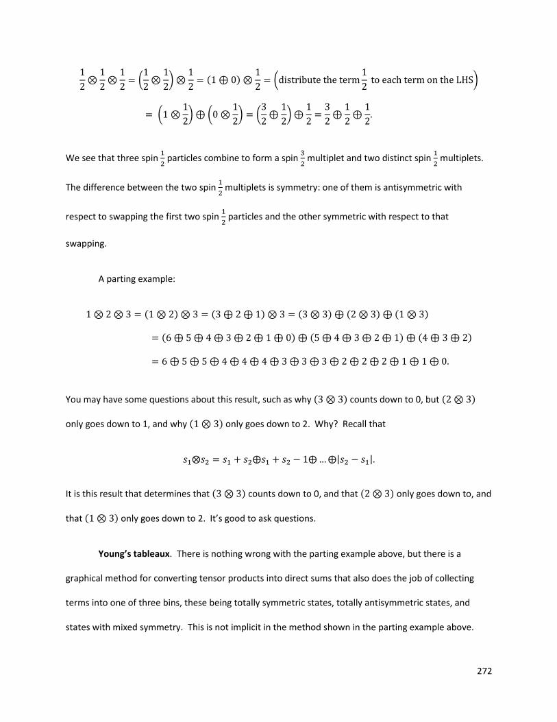
272

(

)

( )

(

)

(

) (

) (

)

We see that three spin

particles combine to form a spin

multiplet and two distinct spin

multiplets.

The difference between the two spin

multiplets is symmetry: one of them is antisymmetric with

respect to swapping the first two spin

particles and the other symmetric with respect to that

swapping.

A parting example:

( ) ( ) ( ) ( ) ( )

( ) ( ) ( )

You may have some questions about this result, such as why ( ) counts down to 0, but ( )

only goes down to 1, and why ( ) only goes down to 2. Why? Recall that

| |

It is this result that determines that ( ) counts down to 0, and that ( ) only goes down to, and

that ( ) only goes down to 2. It’s good to ask questions.

Young’s tableaux. There is nothing wrong with the parting example above, but there is a

graphical method for converting tensor products into direct sums that also does the job of collecting

terms into one of three bins, these being totally symmetric states, totally antisymmetric states, and

states with mixed symmetry. This is not implicit in the method shown in the parting example above.

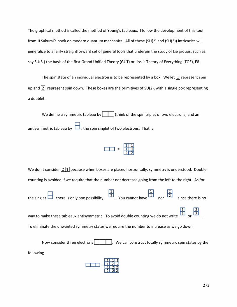
273

The graphical method is called the method of Young’s tableaux. I follow the development of this tool

from JJ Sakurai’s book on modern quantum mechanics. All of these (SU(2) and (SU(3)) intricacies will

generalize to a fairly straightforward set of general tools that underpin the study of Lie groups, such as,

say SU(5,) the basis of the first Grand Unified Theory (GUT) or Lissi’s Theory of Everything (TOE), E8.

The spin state of an individual electron is to be represented by a box. We let represent spin

up and represent spin down. These boxes are the primitives of SU(2), with a single box representing

a doublet.

We define a symmetric tableau by (think of the spin triplet of two electrons) and an

antisymmetric tableau by , the spin singlet of two electrons. That is

We don’t consider because when boxes are placed horizontally, symmetry is understood. Double

counting is avoided if we require that the number not decrease going from the left to the right. As for

the singlet there is only one possibility: . You cannot have nor since there is no

way to make these tableaux antisymmetric. To avoid double counting we do not write or

To eliminate the unwanted symmetry states we require the number to increase as we go down.

Now consider three electrons We can construct totally symmetric spin states by the

following

1 2

1 1

2 2

1 1

2 2

1 1 1 2 1 1

1 2

2 2 2 2 2

=

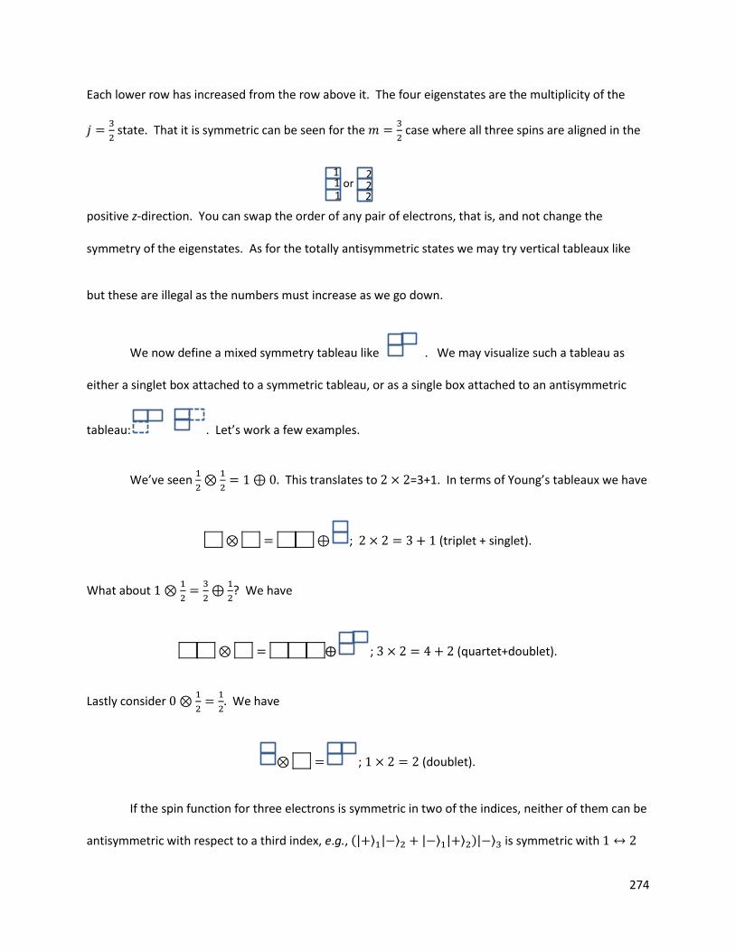
274

Each lower row has increased from the row above it. The four eigenstates are the multiplicity of the

state. That it is symmetric can be seen for the

case where all three spins are aligned in the

positive z-direction. You can swap the order of any pair of electrons, that is, and not change the

symmetry of the eigenstates. As for the totally antisymmetric states we may try vertical tableaux like

but these are illegal as the numbers must increase as we go down.

We now define a mixed symmetry tableau like . We may visualize such a tableau as

either a singlet box attached to a symmetric tableau, or as a single box attached to an antisymmetric

tableau: . Let’s work a few examples.

We’ve seen

This translates to =3+1. In terms of Young’s tableaux we have

; (triplet + singlet).

What about

? We have

; (quartet+doublet).

Lastly consider

We have

; (doublet).

If the spin function for three electrons is symmetric in two of the indices, neither of them can be

antisymmetric with respect to a third index, e.g., (| ⟩ | ⟩ | ⟩ | ⟩ )| ⟩ is symmetric with

1 1 1

2

2 2

or

275

but is neither symmetric wrt or If the number cannot decrease in the horizontal direction

and must increase in the vertical direction, the only possibilities are . The tableau

therefore corresponds to a doublet. Notice that in this scheme we do not consider .

When we were studying the relationship of two spin-

objects between the coupled and

uncoupled representations with ladder operators or Young’s tableaux above, we were really studying

the group SU(2). The two particles could have been the -direction spin labels of two electrons, or they

could have been the labels up and down for the u and d quarks. We now extend our Young’s tableaux

considerations to three primitive spin-

objects—think SU(3). The labels 1, 2 and 3 may stand for the

magnetic quantum numbers of -orbitals in atomic physics or charge states of the pion , or

the , and quarks in the SU(3) classification of elementary particles. A box can assume three

possibilities:

The dimensionality of is 3. Here is some the SU(3) Young’s tableaux algebra if you will:

Antisymmetry:

: : dimensionality 3. Note that in SU(3) we use to distinguish from

: : dimensionality 1 (This state is totally antisymmetrical.)

Symmetry:

1 1 2

1 2

2

1 2

1 3

2 3

1 2

3

276

dimensionality 6.

:

dimensionality 10.

Mixed symmetry:

: : dimensionality 8.

Sakurai develops a general tableaux for representations of SU(3) along with a formula for the

dimensionality of a given tableaux which is not necessary to these notes. Let’s practice with a few

problems.

; (6 symmetric, 3 antisymmetric).

Using the methods we had before Young’s tableaux we would have written

or, changing this to ordinary products and sums: The advantage of Young’s tableaux

is the sum 9 is broken into symmetric, mixed symmetric and antisymmetric bins—there were no mixed

symmetry states in this example. Now let’s check out:

; (8 mixed symmetry, 1 totally antisymmetric). Our old

methods would have

1 1 2

1 2 2

1 3 2

1 1 3

1 2 3

1 3 3

2 2 3

2 3 3

277

It’s the same result as before ( ) but Young’s tableaux tells us more: 8 mixed

symmetry states this time with 1 totally antisymmetric state. Let’s do two more examples.

; (6 symmetric, 8 mixed symmetry). Lastly,

We can refine , , in terms of angular momentum states. We have,

(dimension 7) once (totally symmetric),

(dimension 5) twice (both mixed symmetry),

(dimension 3) three times (one totally symmetric, two mixed symmetry),

(dimension 1) (totally antisymmetric state).

The state is unique, corresponding to the fact that the only product of vectors invariant

under rotation is ( ), which is necessarily antisymmetric. (You should read Sakurai’s fascinating

material connecting the symbol to an antisymmetric state behaving like the ordinary vector

cross product He also discusses how breaks down, noting that it must contain

, but that this is not the only symmetric state; ( ) ( ) ( ) is totally symmetric,

having the transformation properties of Evidently contains both the (seven

states) and (three states).

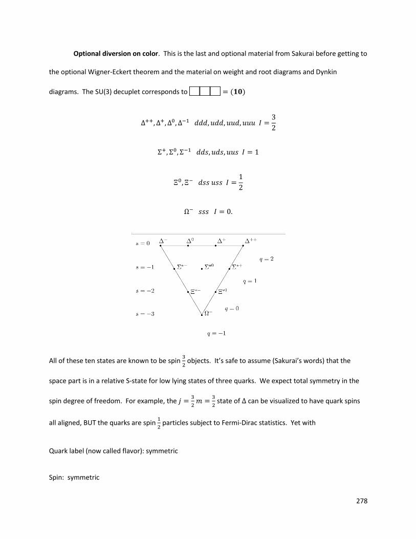
278

Optional diversion on color. This is the last and optional material from Sakurai before getting to

the optional Wigner-Eckert theorem and the material on weight and root diagrams and Dynkin

diagrams. The SU(3) decuplet corresponds to ( )

All of these ten states are known to be spin

objects. It’s safe to assume (Sakurai’s words) that the

space part is in a relative S-state for low lying states of three quarks. We expect total symmetry in the

spin degree of freedom. For example, the

state of can be visualized to have quark spins

all aligned, BUT the quarks are spin

particles subject to Fermi-Dirac statistics. Yet with

Quark label (now called flavor): symmetric

Spin: symmetric

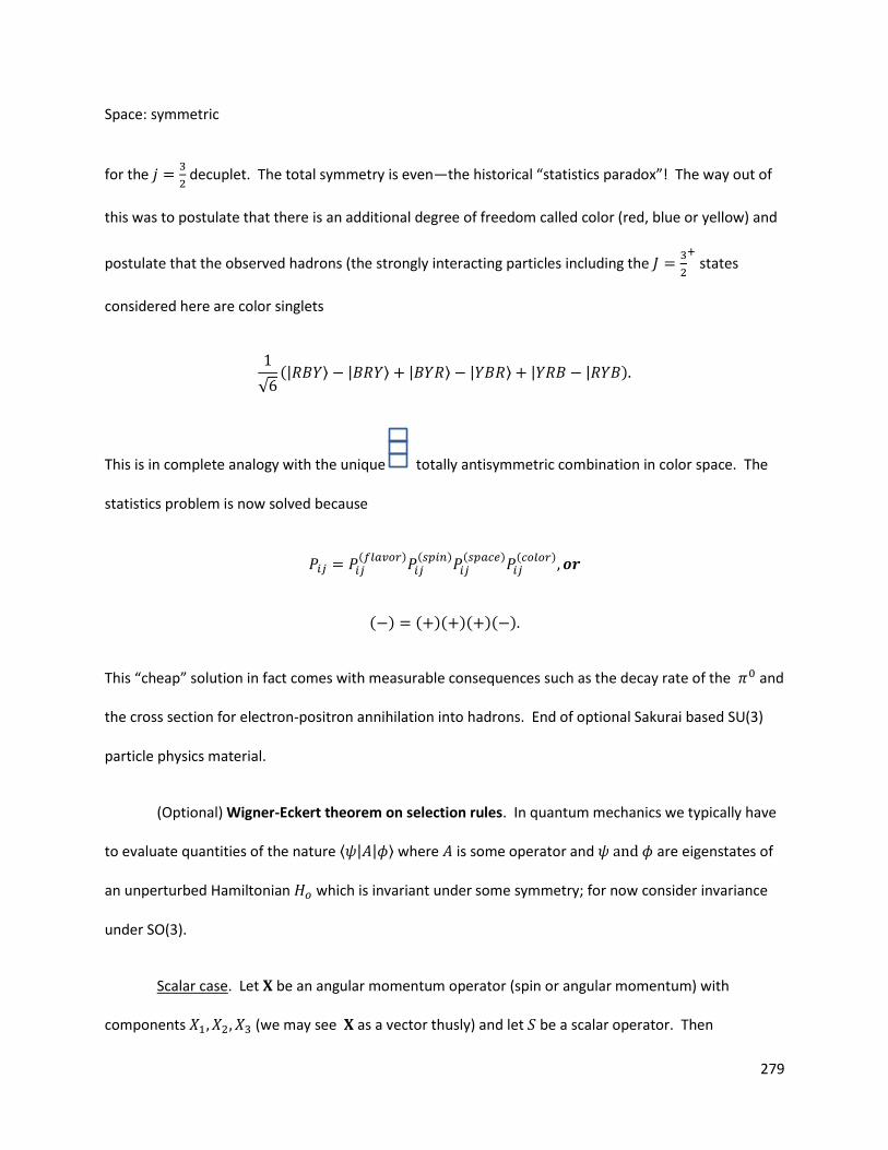
279

Space: symmetric

for the

decuplet. The total symmetry is even—the historical “statistics paradox”! The way out of

this was to postulate that there is an additional degree of freedom called color (red, blue or yellow) and

postulate that the observed hadrons (the strongly interacting particles including the

states

considered here are color singlets

√ (| ⟩ | ⟩ | ⟩ | ⟩ | | )

This is in complete analogy with the unique totally antisymmetric combination in color space. The

statistics problem is now solved because

( )

( )

( )

( )

( ) ( )( )( )( )

This “cheap” solution in fact comes with measurable consequences such as the decay rate of the and

the cross section for electron-positron annihilation into hadrons. End of optional Sakurai based SU(3)

particle physics material.

(Optional) Wigner-Eckert theorem on selection rules. In quantum mechanics we typically have

to evaluate quantities of the nature ⟨ | | ⟩ where is some operator and are eigenstates of

an unperturbed Hamiltonian which is invariant under some symmetry; for now consider invariance

under SO(3).

Scalar case. Let be an angular momentum operator (spin or angular momentum) with

components (we may see as a vector thusly) and let be a scalar operator. Then

280

[ ] , or equivalently wrt SO(3) rotations ( ), ( ) ( ) (Weight and length, for

example, are invariant under rotations.) From the commutator we may extract selection rules that

Unless and , ⟨ | | ⟩ Moreover, this matrix element is independent of , so

that ⟨ | | ⟩ (no summation). Let’s show these conclusion more explicitly.

The condition is a consequence of the vanishing of the commutator [ ] Let me

explain. Consider

⟨ | | ⟩ ( )⟨ | | ⟩

But since is just a scalar (a number), . So

⟨ | | ⟩ ( )⟨ | | ⟩

It must also be that ⟨ | | ⟩ ⟨ | | ⟩ so

( )⟨ | | ⟩ ( )⟨ | | ⟩

Equivalently

( )( )⟨ | | ⟩

Certainly ( ) is positive. So either or ⟨ | | ⟩ is zero. Now for showing that

This follows from [ ] That is, ( ) ( ) Lastly, ⟨ | | ⟩ depends

only on and not on . This is a consequence of the vanishing of [ ] Consider

⟨ | | ⟩ ⟨ | | ⟩ ⟨ | | ⟩

Then

√( )( )⟨ | | ⟩ ⟨ | | ⟩

281

and, recalling that ( ) ,

⟨ | | ⟩ ⟨ | | ⟩ √( )( )⟨ | | ⟩

This is the Wigner-Eckert theorem for scalars. QED.

Vector case. Before getting to the theorem, let’s build up our understanding of vector

operators. Suppose there is an observable that is a vector. That is, its three components in

an orthonormal frame satisfy

[ ] [ ] [ ] ( )

as well as those obtained by cyclic permutations of the indexes and . See complement of

“Quantum Mechanics, Volume Two”, Claude Cohen-Tannoudji, Bernard Diu and Franck Lalöe. (The

material of the vector case is from complement .) To give an idea of what these above commutators

mean, let’s study some examples of vector operators.

The angular momentum is itself a vector. If we let be the above commutators become the

usual angular momentum commutation relations, e.g., [ ] . On the other hand, if we let be

(orbital angular momentum) and be a radius vector, then the relations (A) become

[ ] [ ]

[ ] [ ] [ ]

[ ] [ ] [ ]

For a particle of spin , is given by . In this case the operators are vectors. If we

take into account the fact that all the spin operators (which act only on the spin state space) commute

282

with the orbital operators (which act only in the { } state space), the proof of the commutator

relations (A) follows from our first two examples. On the other hand, operators of the type ( ),

etc., are not vectors, but scalars. Other vector operators could, however, be constructed from these

scalars, e.g., and ( ) etc.

Consider the system (1) + (2) formed by the union of two systems: (1), of state space . And

(2), of spates space . If ( ) is an operator which acts only in , and if this vector (that is, satisfies

(A) with angular momentum vector , of the first system), then the extension of ( ) into state space

is also a vector. (This tensor product stuff is what we have been doing.) For example, for a

two-electron system, the operators , etc. are vectors.

Wigner-Eckert theorem for vectors. We introduce the operators defined by

Using relations (A) we can show that:

[ ]

Let’s check this.

[ ] [ ] [ ] [ ]

Similarly,

[ ]

[ ]

283

Once we have verified the above commutation relations, we can show

[ ]

[ ]

[ ]

[ ]

This kind of algebra, by the way, is the kind of algebra that underlies root and weight diagrams and

Dynkin diagrams that underlie the Standard Model and extensions beyond it using larger Lie groups,

e.g., SU(5) GUT and Lissi E8, which are defunct, but very instructive.

Let’s show that ⟨ | | ⟩ whenever To show this it suffices to note that

and commute (you can prove this to yourself). Therefore the matrix elements of between two

vectors | ⟩ corresponding to two different eigenvalues of of are zero.

For the matrix elements ⟨ | | ⟩ of we shall show that they are different from zero only if

. The equation [ ] indicates that:

Applying both sides of this relation to the ket | ⟩ we obtain

( )| ⟩ |

⟩ | ⟩ ( ) |

⟩

Evidently | ⟩ is an eigenvector of with eigenvalues ( ) . Since two eigenvectors of a the

Hermitian operator associated with different eigenvalues are orthogonal, it follows that the scalar

284

product ⟨ | | ⟩ is zero if Summing up, the selection rules obtained for the matrix

elements of are as follows:

QED. The matrix associated with is diagonal and those associated with have matrix elements only

just above and just below the principal diagonal.

A similar procedure can be adopted to find the selection rules for a tensor operator, .

However the procedure rapidly becomes cumbersome and a more powerful method is required, namely

the Wigner-Eckert theorem (see H F Jones, “Groups, Representation and Physics,” 2nd. Ed. An

irreducible tensor operator is an operator that transforms under rotations according to

( ) ( )

( )| ⟩

(Tensor operators may have more indices .) Stating the result, the Wigner-Eckert theorem states that

⟨ | | ⟩ ( )⟨ || || ⟩

The ( ) are our Clebsch-Gordan coefficients.

Root and Weight diagrams and Dynkin diagrams. Before the theory, let’s begin with an

example that will make the theory transparent. In quantum physics we seek to discover the largest

possible set of commuting hermitian generators because we want to diagonalize as much as

possible. Such a largest possible subset is called the Cartan subalgebra.

285

Example 1—Consider the eight Gell-Mann matrices from Part I, the defining representation of SU(3).

(

) (

) (

)

(

) (

) (

)

(

)

√ (

)

These matrices are hermitian ( ) and traceless. For the Gell-Mann matrices, the Cartan subalgebra is

easy to pick out: and are the only diagonal matrices, and hence they commute: [ ] Therefore we

would say in quantum physics that have simultaneously measurable eigenvalues. The dimension of the

Cartan subalgebra (being 2) is called the rank of SU(3).

Let’s consider the commutator algebra [ ] Find the commutator of the first two matrices:

[ ] (

)(

) (

)(

) (

)

You can check for yourself that [ ] In general, [ ]

where the repeated index implies

summation from and the are the structure constants. For the Gell-Mann matrices, (dividing the

matrices by √ ) we have

√

Any involving an permutation not on this list is zero. Even permutations, e.g., have

the same value. The odd permutations ( ) have the opposite sign. So and

The symbol is said to be totally antisymmetric in

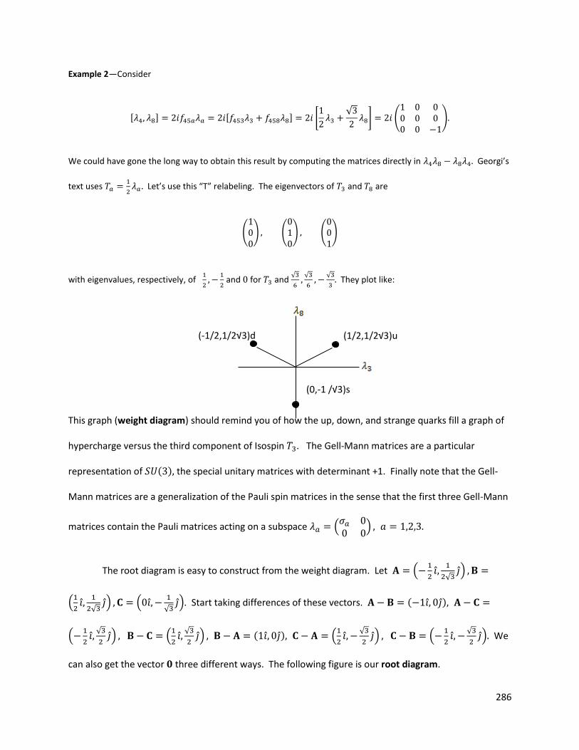
286

Example 2—Consider

[ ] [ ] [

√

] (

)

We could have gone the long way to obtain this result by computing the matrices directly in Georgi’s

text uses

Let’s use this “T” relabeling. The eigenvectors of and are

( ) (

) (

)

with eigenvalues, respectively, of

and for and

√

√

√

They plot like:

This graph (weight diagram) should remind you of how the up, down, and strange quarks fill a graph of

hypercharge versus the third component of Isospin . The Gell-Mann matrices are a particular

representation of ( ) the special unitary matrices with determinant +1. Finally note that the Gell-

Mann matrices are a generalization of the Pauli spin matrices in the sense that the first three Gell-Mann

matrices contain the Pauli matrices acting on a subspace (

)

The root diagram is easy to construct from the weight diagram. Let (

√ )

(

√ ) (

√ ). Start taking differences of these vectors. ( )

(

√

) (

√

) ( ) (

√

) (

√

) We

can also get the vector three different ways. The following figure is our root diagram.

(0,-1 /√3)s

(1/2,1/2√3)u (-1/2,1/2√3)d

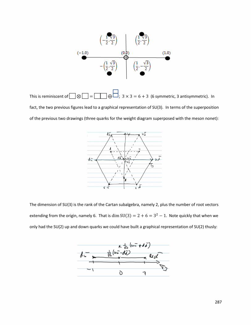
287

This is reminiscent of ; (6 symmetric, 3 antisymmetric). In

fact, the two previous figures lead to a graphical representation of SU(3). In terms of the superposition

of the previous two drawings (three quarks for the weight diagram superposed with the meson nonet):

The dimension of SU(3) is the rank of the Cartan subalgebra, namely 2, plus the number of root vectors

extending from the origin, namely 6. That is ( ) Note quickly that when we

only had the SU(2) up and down quarks we could have built a graphical representation of SU(2) thusly:

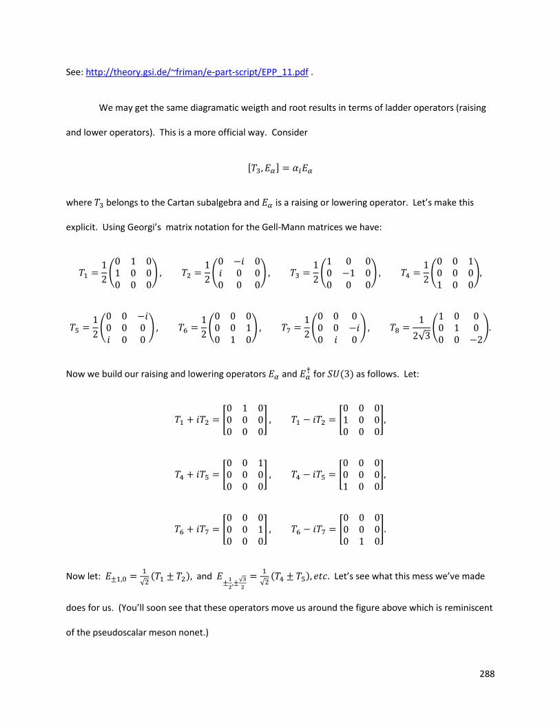
288

See: http://theory.gsi.de/~friman/e-part-script/EPP_11.pdf .

We may get the same diagramatic weigth and root results in terms of ladder operators (raising

and lower operators). This is a more official way. Consider

[ ]

where belongs to the Cartan subalgebra and is a raising or lowering operator. Let’s make this

explicit. Using Georgi’s matrix notation for the Gell-Mann matrices we have:

(

)

(

)

(

)

(

)

(

)

(

)

(

)

√ (

)

Now we build our raising and lowering operators and for ( ) as follows. Let:

[

] [

]

[

] [

]

[

] [

]

Now let:

√ ( ) and

√

√ ( ) Let’s see what this mess we’ve made

does for us. (You’ll soon see that these operators move us around the figure above which is reminiscent

of the pseudoscalar meson nonet.)

289

[ ] [ ] [ ]

[

]

So the eigenvalue is Consider [ ] [ ] ( )

for this case. So we get the point ( ) of our meson nonet. Let’s try a few more.

[ ] ( ) [ ] ( )

Now we have the point ( ) of our nonet. Let’s proceed to:

[ ] ( )

[ ]

√

( )

√

and finally,

[ ] [ ] [ ]

the three points at the origin. Doing all the cases gives us our complete nonet root diagram. Let me just

say that the Killing form is used to transform the Cartan subalgebra into an orthonormal basis. We’ll get

to that in a moment, but first let me show you yet one other way to build our nonet via the adjoint

representation of SU(3).

The adjoint representation of ( ) The structure constants themselves generate a

representation of the algebra called the adjoint representation. That is, we may define a set of

matrices [ ] [ ] just as the Gell-Mann matrices do.

Example 3—Let’s see.

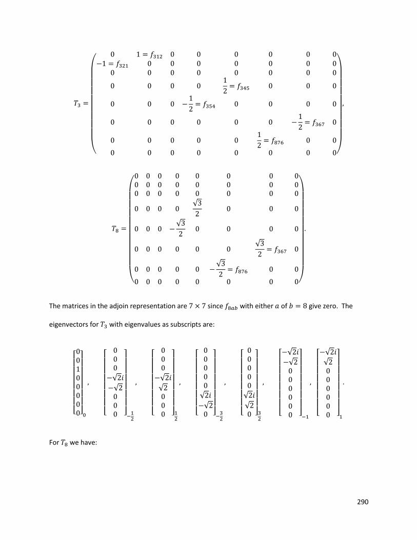
290

(

)

(

√

√

√

√

)

The matrices in the adjoin representation are since with either of give zero. The

eigenvectors for with eigenvalues as subscripts are:

[ ]

[

√

√ ]

[

√

√ ]

[

√

√ ]

[

√

√ ]

[ √

√ ]

[ √

√ ]

For we have:

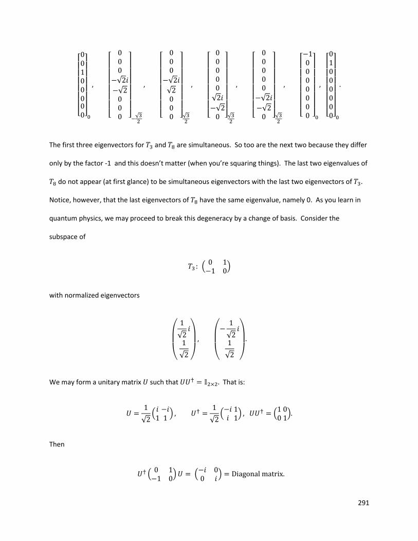
291

[ ]

[

√

√ ]

√

[

√

√ ]

√

[

√

√ ]

√

[

√

√ ]

√

[ ]

[ ]

The first three eigenvectors for and are simultaneous. So too are the next two because they differ

only by the factor -1 and this doesn’t matter (when you’re squaring things). The last two eigenvalues of

do not appear (at first glance) to be simultaneous eigenvectors with the last two eigenvectors of

Notice, however, that the last eigenvectors of have the same eigenvalue, namely 0. As you learn in

quantum physics, we may proceed to break this degeneracy by a change of basis. Consider the

subspace of

(

)

with normalized eigenvectors

(

√

√ )

(

√

√ )

We may form a unitary matrix such that That is:

√ ( )

√ ( ) (

)

Then

(

) (

)

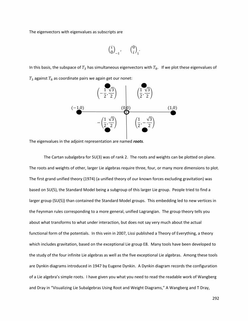
292

The eigenvectors with eigenvalues as subscripts are

( )

( )

In this basis, the subspace of has simultaneous eigenvectors with If we plot these eigenvalues of

against as coordinate pairs we again get our nonet:

(

√

) (

√

)

( ) ( ) ( )

(

√

) (

√

)

The eigenvalues in the adjoint representation are named roots.

The Cartan subalgebra for SU(3) was of rank 2. The roots and weights can be plotted on plane.

The roots and weights of other, larger Lie algebras require three, four, or many more dimensions to plot.

The first grand unified theory (1974) (a unified theory of our known forces excluding gravitation) was

based on SU(5), the Standard Model being a subgroup of this larger Lie group. People tried to find a

larger group (SU(5)) than contained the Standard Model groups. This embedding led to new vertices in

the Feynman rules corresponding to a more general, unified Lagrangian. The group theory tells you

about what transforms to what under interaction, but does not say very much about the actual

functional form of the potentials. In this vein in 2007, Lissi published a Theory of Everything, a theory

which includes gravitation, based on the exceptional Lie group E8. Many tools have been developed to

the study of the four infinite Lie algebras as well as the five exceptional Lie algebras. Among these tools

are Dynkin diagrams introduced in 1947 by Eugene Dynkin. A Dynkin diagram records the configuration

of a Lie algebra’s simple roots. I have given you what you need to read the readable work of Wangberg

and Dray in “Visualizing Lie Subalgebras Using Root and Weight Diagrams,” A Wangberg and T Dray,

293

Department of Mathematics, Oregon State University, Corvallis, Oregon 97331, 15 March 2008. You

may find this brief but explicit article at:

http://www.math.oregonstate.edu/~tevian/JOMA/joma_paper_softlinks.pdf . This material is brought

to life by the authors at http://www.math.oregonstate.edu/~tevian/JOMA/joma_paper_three.html .

You can see the plotting being done by JAVA script. These authors show you how to build Dynkin

diagrams, and how to use them to help you study subalgebras. I have pitched my copy of Georgi in the

trash, something I should have done years ago. H F Jones is now far more readable. This concludes the

“Lie” program tying differential equations (ordinary and partial, linear and nonlinear) with algebra and

global and local topology with physics.

294

Part V.I Fractional calculus. Differentiation and integration can be generalized beyond

integrating and differentiating in integer steps, e.g., 1st derivative, 2nd derivative, and so on. I

recommend “The Fractional Calculus, Theory and Applications of Differentiation and Integration to

Arbitrary Order,” K. B. Oldham and J. Spanier, Dover, 1974. It is far more general and applied and full of

centuries of history than a website I found on this subject. Nevertheless, the notes I made from the

website provide a good beginning to Oldham and Spanier.

Consider ( ) If you take derivatives you get:

( ) (We’ll soon see

that if is a negative integer, this leads to integrations.) So why don’t we replace with where is

not necessarily a positive integer? Then,

In fact any function that is expressible as a linear

combination of exponential functions can be differentiated likewise:

[

]

( ) ( )

Since ( )

(

)

The differential operator shifted the phase of the cosine function (ditto the sine function).

Now consider that a very large class of functions have Fourier representations:

( )

√ ∫ ( )

( )

√ ∫ ( )

Here and are Fourier transforms of each other. Then differentiating ( ) by results in

295

( )

√ ∫ ( )( )

Evidently the Fourier transform of the generalized th of ( ) is ( ) ( ) This approach to the

fractional calculus has pathologies. With this approach, how do we determine the half-derivative of

( ) There is no Fourier representation for this open-ended function. We could chose a finite

interval, but which one? Let’s turn back to the definition of differentiation.

( )

( ) ( )

Repeat once to get:

( ) ( )

( ( ) ( )

)

( ) ( ) ( )

Repeat again to get:

( ) ( ) ( ) ( ) ( ) ( )

( ) ( ) ( ) ( )

Repeating times yields

( )

∑( ) (

) ( )

(1)

Indeed if ( ) (dropping all powers of or higher):

[ ( ) ( ) ]

[ ]

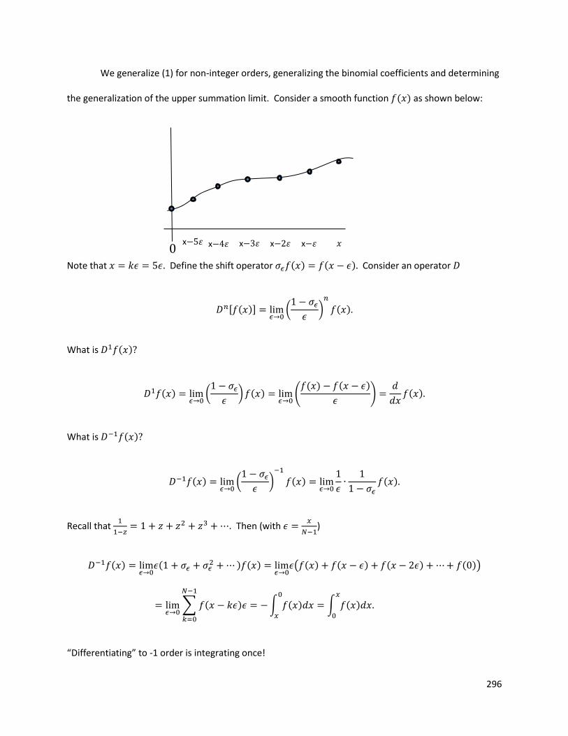
296

We generalize (1) for non-integer orders, generalizing the binomial coefficients and determining

the generalization of the upper summation limit. Consider a smooth function ( ) as shown below:

Note that Define the shift operator ( ) ( ) Consider an operator

[ ( )]

(

)

( )

What is ( )

( )

(

) ( )

( ( ) ( )

)

( )

What is ( )

( )

(

)

( )

( )

Recall that

. Then (with

)

( )

( ) ( )

( ( ) ( ) ( ) ( ))

∑ ( )

∫ ( )

∫ ( )

“Differentiating” to -1 order is integrating once!

x 휀 x 휀 x 휀 x 휀 x 휀 𝑥

297

Regarding equation (1), if is a positive integer, all of the binomial coefficients after the first

are zero ( ( ) For negative or fractional values of the binomial coefficients

are non-terminating. We must sum over the specified range. The upper limit should be

yielding:

( )

∑ ( ) (

) ( )

|( )

|

(1a)

What do we do about ( )

( ) when is not an integer? Enter the gamma function. For integers

( ) ( )

It is a consequence of the general gamma function for complex-valued arguments, which is

( ) ∫

Most special functions of applied mathematics arise as solutions to differential equations. Not so the

gamma function—at least not yet (Hölder’s theorem). From the following integral

∫ ( )

( ) ( )

√

( )

∫ ( )

Thanks to the ( ) argument, we have generalized the definition of the factorial to negative and/or

positive half-integers, e.g., (

) √ But we have actually done better than this. Now that the

factorial of all half-integers is defined, we can compute the factorial of quarter-integers, sixteenth

integers,…,so that, using the binary representation of real numbers, and using the identity the

( ) ( ) we actually have a well-defined factorial function for any real number, otherwise

known as the gamma function: ( ) ( ) The recurrence relationship is ( )

298

( ) The reflection relation is ( ) ( ) ( ) One could write volumes on the gamma

function. Now we can generalize (1a) to

( )

∑ ( )

( )

( ) ( )

|( )

|

(2)

Ordinary differentiation is local, integration is not local, nor is our generalized definition of

differentiation/integration (2) (See Oldham and Spanier). If is integer-valued, the binomial coefficients

for all vanish past and in the limit as goes to zero the values of ( ) with nonzero

coefficients converge on keeping the generalized operator local. In general, however, the binomial

expansion has infinitely many non-zero coefficients, so the result depends on the value of all the way

down to (Look up Huygens’ Principle and the sharp propagation of light in three dimensions.)

Choosing equation (2) becomes

( )

∑( )

( )

( ) ( )

| |

(3)

Let’s go for a test drive with ( ) and

√ [

( )

( )

(

)

( )

( ) (

)

( )

( ) (

[

]

)( ) (

[

]

)( )]

√ [

]

299

where the factorials are in terms of the gamma function. Recall that we used (

) With

(

)

√ √

√ (

)

Then really have:

√ √

√

√ ( )

√

√

√

That is,

√

(4)

If we play around a bit with regular calculus we observe the pattern

( ) In our

generalized framework we have

( )

(5)

Then, paradoxically, using equation (5), the half derivative of a constant is:

( )

√

√

300

We have to be careful and think about local versus nonlocal behavior. Equation (5) gives no hint on non-

locality, as opposed to equation (3) which depends on what is doing locally. This issue is cleared up by

considering the half derivative of the exponential function Using equation (5) we get

(

)

√ (

)

Wouldn’t we have expected this derivative of the exponential function to equal itself? A plot of the

above series versus shows that the two graphs converge asymptotically at large However near the

origin, the series blows up whereas passes smoothly through Consider the integrals

∫

∫

The left hand integral shows that when we say is the derivative of

we are implicitly assuming

This is consistent with our derivation of (3). HOWEVER, when we say that is the derivative of

we are saying that so that Thus for each of the two above integrals/derivatives we

have tacitly assumed different ranges. The fix is to go back to equation (2) and replace with

Now we’re cooking:

( )

∑( )

( )

( ) ( )

One point of this section is to out the glaring omission of calculus with other than integer order

differentiation and integration, it can be real-value-ordered, even complex-value-ordered. There are

also strong applications of fractional calculus to the problems of transport and diffusion processes such

as neutron migration and flow through porous materials. Talking about diffusion processes…

301

Part V.II Stochastic differential equations (SDEs), random walks and the Itô calculus. My goal

here is to prove a theorem concerning quadratic variation. Why? For practical ends I assure you. How

does one integrate a function in which some of the terms are stochastic? In difference form consider

( ) ( )

where ( ) the normal distribution with mean 0 and standard deviation 1. We start at

and head to ending up at some unknown value of What would be our

“expectation” of (What is the mean of What is the standard deviation of The physicists

answered this question employing Monte Carlo methods requiring computers. With a computer we

throw a dart, so-to-speak and pick a number between 0 and 1 according to ( ) (or some other

distribution). We advance and repeat, generating a path until we arrive at The we start the

process from scratch, repeating it many times over so that we obtain a numerical estimate of the mean

and standard deviation of The mathematicians did things nice and proper in a measure-theoretic

framework. Is there a middle ground? Yes. The material presented below. Along the way we will see

applications to diffusion and high finance.

On quadratic variation (this first portion excerpted from the Feynman lectures). Let be the

net distance traveled in steps (each with time and speed ) of a drunken sailor in one-dimension.

Then, (with expectations, or means in brackets),

⟨ ⟩

If the sailor steps to the right, then we have

( ) ( )

( )

If the sailor steps to the left (with equal probability) then we have

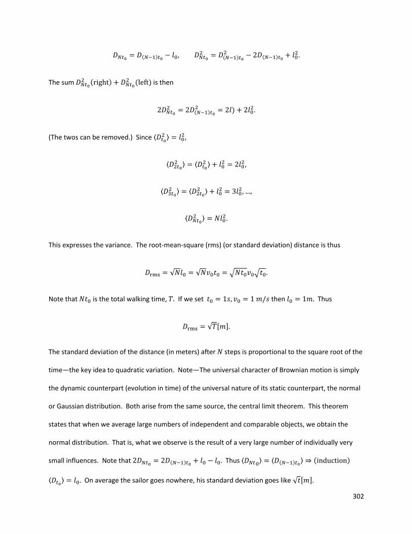
302

( ) ( )

( )

The sum ( )

( ) is then

( )

)

(The twos can be removed.) Since ⟨ ⟩

⟨ ⟩ ⟨

⟩

⟨ ⟩ ⟨

⟩

⟨ ⟩

This expresses the variance. The root-mean-square (rms) (or standard deviation) distance is thus

√ √ √ √

Note that is the total walking time, If we set then Thus

√ [ ]

The standard deviation of the distance (in meters) after steps is proportional to the square root of the

time—the key idea to quadratic variation. Note—The universal character of Brownian motion is simply

the dynamic counterpart (evolution in time) of the universal nature of its static counterpart, the normal

or Gaussian distribution. Both arise from the same source, the central limit theorem. This theorem

states that when we average large numbers of independent and comparable objects, we obtain the

normal distribution. That is, what we observe is the result of a very large number of individually very

small influences. Note that ( ) Thus ⟨ ⟩ ⟨ ( )

⟩ ( )

⟨ ⟩ On average the sailor goes nowhere, his standard deviation goes like √ [ ]

303

Necessary review of probability theory. Let’s start by reviewing moments. If ( ) is a

probability density function (density or distribution) the first moment about the origin (the center of

mass) is

[ ] ∫ ( )

The first moment about is [ ( )] The second moment (the VARIANCE) about the mean is

[( ) ] [ ] [ ] [ ] [ ( [ ]) ] The th

moment about the mean is defined by

[( ) ] ∫ ( ) ( )

Naturally, the th the moment about the origin is [ ] In general [ ] [ ( [ ]) ]

The Moment Generating Function (MGF). Let be a random variable. The MGF of is

( ) [ ] at all values of for which the expected value exists. In integral form,

( ) ∫ ( )

Example 1—Let our density be

( ) {

( ) ∫

Theorem (no proof)—The th derivative of the MGF obeys ( )( ) ∫ ( ) [ ]

NOTE:

the expectation [ ] are taken with in ( )

304

Example2—For example 1: ( )( )

( ) so ( )( ) [ ] This gives our mean and

variance. The mean is [ ] ( )( ) The variance is ( ) ( )

( )( )

Now we will denote the MGF by:

( ) [ ] ∫ ( )

Note that if and are independent random variables, ( ) ( ) Think convolution.

( ) [ ] [ ]

[ ] ( )

where ( ) denotes the round off error. As before ( )( ) [ ] for the kth derivative. Consider

( ) ( )

√

(A) a normal density with mean 0 and standard deviation 1. Let

then we have ( ) being defined by

( )

√

(

)

(Drop the primes.) Getting back to the MGF for ( )

( ) ∫ ( )

√ ∫

Completing the square:

( )

so (B)

( )

√ ∫

√ ∫

( )

√

305

The last integral is so because with we get ∫

. Thus for

( ) ( ) ∫ ( )

√

[ ]

Combining (A) with (B) we get:

[ ( )] [ ] ( ) [ ( )]

but now for the normal density ( ) We will see this result when we deal with a simple stochastic

differential equation (SDE) for Brownian motion (or stocks). Let

( )

(

)

( )

( )

∑ ( )

So the variance of x with this density is [ ] ( ) and [ ] …, and so on by

reading off the successive terms (the statistical moments about the mean) from the MGF series. Thus

the variance of is [ ] ( ) [ ] ( [ ]) Let’s put all of this crap together

for once and all.

A Brownian motion (drunken sailor). For each the random variable ( ) ( )

( ) is the (drunken) increment in time [ ] where the increments are Gaussian increments with

mean zero, variance and with density

( )

√

( )

( )

√

√

That is, ( ) ( ) ( √ ) (What does this? Drunken sailors walking in one or

more dimensions, neutrons diffusing in a star, and approximately stock prices. Physicists extract the

mean (first moment about the origin) and variance (second moment about the mean) by Monte Carlo.

306

By definition we have set [ ( )] By definition we have set ( ) √ Then plugging

into the definition of variance of ( ), we have ( ( )) [ ( ) ( [ ( )]) ] [ ( )]

( ) Plugging into the definition of variance for ( ( )) we have ( ( )) [ ( )

( [ ( )]) ] [ ( ) ] [ ] I got the term by translating the result for

[ ] ( ) [ ] ( [ ]) above. (Remember that in a Brownian process

(Feynman’s drunken sailor So )

Thus for and ( ( )) ( ( )) [ ( )] With a

fine enough partition of of a time interval [ ] we see what is called the quadratic variation of

Brownian motion.

∑[ ( )] ∑

Theorem—∑ [ ( )] ∑

in probability | | (Proof see

above—screw measure theory in the absence of context).

This result is used in a key theorem of the Itô calculus and in measure theoretic integration theory. Let’s

get to Itô’s lemma. (A Weiner process/Brownian motion are the same thing.)

Itô’s lemma. Given a Weiner process ( )√ , let ( ) ( ) Then

[ ] since ( ) [ ] and ( ) . Thus √ ( ) √ . Say

( ) with no stochastic attribute for now. Then

( )

For small

Now suppose ( ) ( ) ( )√ Then

307

( ) ( ) ( )

With

, ( ) Thus [ ] ( ) Also ( )

[ ( ) ( [ ( )) ) ] (we’ve just derived this above, but now the time

interval is included). As a result of this (and for small ) we may treat as non-

stochastic with mean as (We dropped the variance term of thanks to the quadratic

variation of the random walk we are working with.) With ( ) taking limits as

we get (KEEPING ONLY FIRST POWERS OF DIFFERENTIALS, e.g., but dropping )

Cool result. With we get:

( )

(

)

So what? Itô’s lemma allows us to deduce the moments of an arbitrary function ( ) where is

following a stochastic Brownian motion! This is powerful. Stock prices can be approximated by

Brownian motion. Derivative instruments are financial instruments defined as functions of time and

the stochastic (Brownian process) price . The drift rate of ( ) is

(and looking at the coefficient for ) the variance rate is

308

This is one of the theoretical bases for pricing derivatives (sensible derivatives based on some stochastic

process which doesn’t have to be Brownian, a Langevin process say. Derivatives based on BS are

dangerous.) Other ways to extract moments are Monte Carlo simulation (you must have good random

number generators), binary trees, and trinary trees (equivalent to finite difference methods for PDEs).

There is a beautiful mapping of the heat equation to the Black-Scholes equation for call and put options.

Example 3—A variation of an Orhstein-Uhlenbeck (father of the H-bomb) mean reverting process. Let

( ) ( ) √ ( )

Find the mean, variance and probability density function of the process analytically—no computers!

⟨ ⟩ ⟨ ⟩

since ⟨ ⟩

∫ ⟨ ⟩

⟨ ⟩ ∫

⟨ ⟩

⟨ ⟩

Thus, ⟨ ( )⟩ ⟨ ⟩ the mean is ⟨ ⟩ ⟨ ⟩

The variance is [ ] ⟨ ⟩ ⟨ ⟩ Recall

Itô’s lemma. With ( ) ( ( ) ) ( ( ) )

[ ( ) ] (

)

Comparing the equation for ( ) at the top with the equation just above this line, we see that

√

If [ ( ) ] say, (with ) then

309

(

) ( )

Plugging our results for and into the equation above leads to

( ) √

So,

⟨ ⟩ ⟨ ⟩ √ ⟨ ⟩

⟨ ⟩ ⟨ ⟩

Then

⟨ ⟩

⟨ ⟩

Thus with integrating factor: ∫

we have

⟨ ⟩

⟨ ⟩

So

[⟨ ⟩ ] Integrating we get:

∫ ⟨ ⟩ ∫

[

( )]

So ⟨ ⟩ ( ) where is a constant. Now the initial condition ⟨ ( )⟩ ⟨ ⟩

So, [ ] ⟨ ⟩ ( ) ⟨ ⟩ Therefore [ ] [ ] ( [ ])

( ⟨ ⟩ ) ⟨ ⟩

(⟨ ⟩ ⟨ ⟩

) So [ ] [

] We seek the density associated with the corresponding Fokker-Planck equation.

310

Some (optional) Background on Fokker-Planck equation. (“A modern course in statistical

physics,” L. E. Reichl, University of Texas Press, 1980.) (Graduate school level statistical physics.) The

Master equation is

∫{ ( ) ( ( ) ( ) ( )}

where is the density for a Brownian particle and accounts for the conditional, or transmitted

density per unit time. This process is stationary if ( ) ( ) (no time dependence). If the

transitions are small we get the Fokker-Planck equation

[ ( ) ( )

[ ( ) ( )]]

Where is the th order jump moment. If particle collisions are restricted to being binary, we get the

restricted Boltzmann (Vlasov) equation:

∫ ∫ | | [ ](

)

Detailed balance means This leads to the H-theorem (which leads to the approach to

equilibrium). A Hamiltonian may supply the transition matrix, e.g., BBGKY. END.

The Fokker-Planck equation (FPE) governs the transport of the probability density for a given

stochastic process. For a general diffusion process,

This process maps to the FPE as

( )

( )

311

For our Orhstein-Uhlenbeck process √ we have

√ and

( )

( )

We shall solve this PDE by the Fourier transform method.

[

] [

( )]

[

( )]

[

] ( )

where

( ). Note that [

] ( ) ( )[ ( )] ( ) [

], where [ ( )]

∫ ( ) ( )

So our equation becomes

a first-order ODE. The method of characteristics is appropriate. Let be constant along the

characteristics

( )

( )

Then,

312

Along the characteristics we require the reparameterization

This implies that

or

along the characteristic. Check: Plug

into the equations for

and

Now if constant along the characteristic, we see that our pair of equations above

becomes

Recovering the original equation. Therefore along these characteristics a general solution exits as

( ) We get

Thus Also

313

Thus . So ( )

and

WLOG let Let

then since ( ) and ( ) set

( )

( )

The general solution can be written as ( ) where ( ) is an arbitrary function. We have

( )

( ) With initial condition (I.C.) ( | ) ( ) we get

( )

( )

This implies that ( )

Finally, ( | )

( )

). Invert this

( | ) ∫ ( )

∫ ∫

( ) ( )

[ ( ) ( )]

∫ [ ( )] [ ( )]

By convolution. FINALLY

( | )

√ ( ) ( ( )

( )

(Abstraction for the sake of efficient exploration is fine if it has good foundations). Thanks. A. Alaniz.

314

Some final thoughts. We humans have compiled a pretty good smallish set of engineering

manuals that span from the minutia of particles and fields all the way to the observable cosmos and all

things in between that we can engineer and/or model from space stations to play stations and DNA logic

gates, stars and nuclear devices, weather patterns and stock markets. For me these notes mark my

attempt to understand as much of observational phenomenology as possible with the least amount of

mathematical machinery that maximizes the unity of ideas while minimizing prescriptive, voodoo

mathematics. Without, however, having a background covering the gamut of nuclear weapons design

physics from high explosive physics to radiation transport and the numerical methods techniques

inherent in simulating these kinds of weapons, my experience at DARHT, in molecular dynamics and

financial physics ranging from natural gas derivatives to climatology, and much other sundry experience,

these notes would be no more to me than a meatless skeleton devoid of any intuition that comes from

painstaking struggle and eventual hands on familiarity. At a minimum, core graduate physics courses

supply sufficient foundations.

The extremes of our knowledge small and large apply far beyond the everyday engineering

world. We don’t need to know about quarks to make refrigerators or lunar bases or to design genetic

corrections. Isn’t a smallish codification of observation what many physicists have dreamt of? In this

sense there is a great measure of completeness for me in these notes bounding what we know, but I

also know that the extremes of our knowledge are vanishingly small. The Lie groups that we use to

codify known particles and fields can be embedded in far larger, far richer Lie groups allowing us to

theorize about possible extensions of our universe, or other possible universes. The border separating

what we know, moreover, from what might be possible is our empirical knowledge, and it’s getting ever

harder to generate fundamental data. The LHC is a monster in terms of international cost. Progress will

be made, but is it asymptotically bound to practical limits from cost to technology? Indeed progress

315

might also be bound by physics itself, if, say, we build a big enough machine to start making little,

rapidly evaporating black holes.

Beyond the semi-intuitive theoretical extensions of our Standard Model to larger, higher-

dimensional Lie groups, (beyond this set of “core” notes) there are other relatively intuitive extensions

to consider. There is the text by M. Nakahara, “Geometry, Topology, and Physics”, 2nd ed. It reaches out

“linearly” to generalizations of the covariant derivative for example, but it also tickles the edge of chaos

where theoretical physics and pure mathematics merge into the wild, wild west. “The Knot Book, An

Elementary Introduction to the Mathematical Theory of Knots,” C. C. Adams, treating mostly two-

dimensional knots in our usual three-dimensional space seems to me to be somewhat like genetics.

How many different genera has nature concocted from a set of merely four letters? How far will we

humans and our descendants be able to take this four letter alphabet beyond cats who glow with the

genes of bioluminescent sea life? How many different classification schemes will lead to light in knot

theory? By surfaces, by simplexes, by crossing numbers, by Conway’s notation, by polynomials,

etcetera, etcetera, etcetera? How much of this is mathematics? How much of this stuff at and beyond

three dimensions is actually taken advantage of by physics? Read up on, “The Jones polynomial and

quantum field theory,” by E. Witten, Communications in mathematical physics, 121, 351-399 (1989).

How many ways can string theorists fold higher dimensional manifolds? The degrees of freedom of

mathematics seem to greatly exceed the explanatory needs of physics running up as it is against brick

walls in costs and potential deserts of no new physics beyond the Standard Model up to some unknown

energy threshold.