Embed Size (px)
Citation preview
MATH 245 NOTES: SYZYGIES
AARON LANDESMAN
CONTENTS
1. Introduction 32. 4/3/17 42.1. Introducing notation 42.2. Enter Brill-Noether theory 63. 4/10/17 83.1. Constructing the Eagon-Northcott complex 84. 4/12/17 124.1. Fitting ideals 124.2. The Buchsbaum Eisenbud criterion 135. 4/14/17 175.1. Rational normal curves 176. 4/19/17 196.1. Picard group of Mg 227. 4/21/17 237.1. Grothendieck Riemann Roch 237.2. Hurwitz Divisor 268. 4/24/17 289. 4/26/17 329.1. Graded Tor 329.2. The Koszul complex, revisited 329.3. Kernel Bundles 3310. 4/28/17 3510.1. Hirschowitz-Ramanan 3911. 5/8/17 4012. 5/10/17 4312.1. Computing the second class 4412.2. Computing the first class 4512.3. The factor of k− 1 4613. 5/12/17 4713.1. K3 Surfaces 4914. 5/15/17 5014.1. Interlude on the Picard group of a K3 surface 50
1
2 AARON LANDESMAN
14.2. Stability of Lazarsfeld-Mukai bundles 5315. 5/17/17 5415.1. Hirzebruch-Riemann-Roch for K3 surfaces 5415.2. Recollection of Brill-Noether theory 5515.3. Brill Noether on K3 surfaces 5715.4. Deformation theory of Hilbert schemes 5816. 5/22/17 5917. 5/24/17 6217.1. The construction ofWr
d(C) 6218. 5/26/17 6618.1. Wrapping up the Petri map 6618.2. Return to syzygies 6719. 5/31/17 7020. 6/2/17 7321. 6/5/17 7522. 6/7/17 7822.1. An alternate construction of F 79
MATH 245 NOTES: SYZYGIES 3
1. INTRODUCTION
Michael Kemeny taught a course (Math 245) on Syzygies at Stan-ford in Spring 2017.
These are my “live-TEXed“ notes from the course. Conventionsare as follows: Each lecture gets its own “chapter,” and appears inthe table of contents with the date.
Of course, these notes are not a faithful representation of the course,either in the mathematics itself or in the quotes, jokes, and philo-sophical musings; in particular, the errors are my fault. By the sametoken, any virtues in the notes are to be credited to the lecturer andnot the scribe. 1 Please email suggestions to aaronlandesman@gmail.
com.
1This introduction has been adapted from Akhil Matthew’s introduction to hisnotes, with his permission.
4 AARON LANDESMAN
2. 4/3/17
Today, we’ll discuss why people care about syzygies. Syzygies goback to mid-19th century geometric invariant theory.
A syzygy is simply a relation among the equations of a projectivevariety. This goes by to Sylvester in 1850.
Example 2.1 (Syzygies of the twisted cubic). Consider the map
ν : P1 → P3
[u; v] 7→ [u3,u2v,uv2, v3
].
The twisted cubic X := ν(P1), the 3-Veronese embedding of P1 in P3.We can note also that X is the scheme theoretic intersection of
f := yw− z2
g := yz− xw
h := xz− y2
There are two syzygies:
xf+ yg+ zh = 0
yf+ zg+wh = 0.
2.1. Introducing notation. For the remainder of the course, we fixthe following notation. Consider S := C [x0, . . . , xn], a graded ring inn+ 1 variables. Let Sd denote the homogeneous polynomials in S ofdegree d. Let M be a finitely generated graded module over S. ForC a curve, we will let g denote the genus.
Example 2.2. Let the twisted module S(−n) be the S-module de-fined so that S(−n)d := Sd−n. Note that as a module (without agrading) this is isomorphic to S.
Definition 2.3. A graded S module M is free if one can write M =⊕nS(−n)⊕bn .
Definition 2.4. A resolution F• →M is minimal if each δi : Fi → Fi−1takes a basis of Fi to a minimal set of generators of im (δi).
Theorem 2.5 (Hilbert syzygy theorem, 1890). Let M be a finitely gen-erated graded module over S := C[x0, . . . , xn]. Then there exists a uniqueminimal free resolution(2.1)0 M F0 F1 · · · Fn+1 0
δ1 δ2 δn+1
of length at most n+ 1.
MATH 245 NOTES: SYZYGIES 5
We’ll prove this on Friday.
Definition 2.6. If M is a finitely generated graded S module, thenthe Hilbert function is the map
fm : Z→ Z
d 7→ dimCMd.
Remark 2.7. One can verify that the Hilbert function is eventuallypolynomial, and one defines the Hilbert polynomial to be this poly-nomial.
Definition 2.8. Let F• be the minimal free resolution ofM. Then, say
Fi = ⊕jS (−i− j)bij .
These bij are the Betti numbers associated to f.Define
∆j :=∑i≤j
(−1)j bj−i,i,
to be the alternating sum of the diagonal elements of the Betti table,which is the table containing bij in position (i, j).
Lemma 2.9. We have
fm(d) =∑j
(−1)j+1∆j
(n+ d− j
n
).
In this formula, we have(an
)= 0 if a < n.
Proof. Omitted.
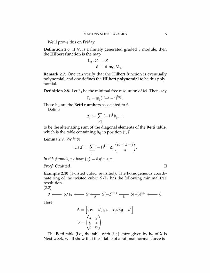
Example 2.10 (Twisted cubic, revisited). The homogeneous coordi-nate ring of the twisted cubic, S/IX has the following minimal freeresolution.(2.2)
0 S/IX S S(−2)⊕3 S(−3)⊕2 0.A B
Here,
A =[yw− z2,yz− xy, xy− z2
]B =
x yy zz w
.
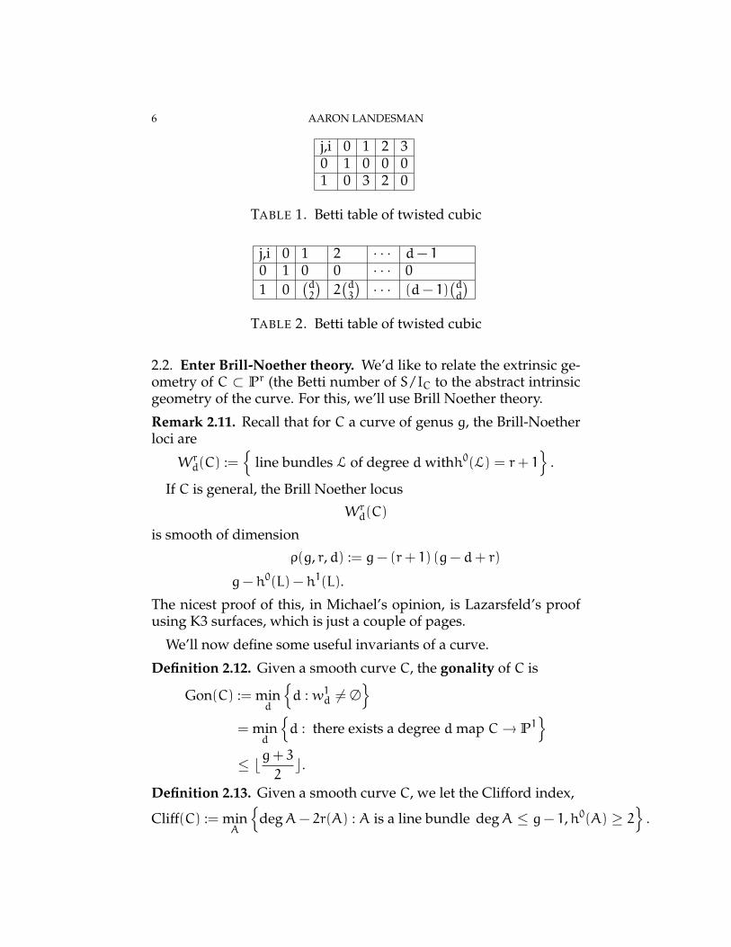
The Betti table (i.e., the table with (i, j) entry given by bij of X isNext week, we’ll show that the 4 table of a rational normal curve is
6 AARON LANDESMAN
j,i 0 1 2 30 1 0 0 01 0 3 2 0
TABLE 1. Betti table of twisted cubic
j,i 0 1 2 · · · d− 10 1 0 0 · · · 01 0
(d2
)2(d3
)· · · (d− 1)
(dd
)TABLE 2. Betti table of twisted cubic
2.2. Enter Brill-Noether theory. We’d like to relate the extrinsic ge-ometry of C ⊂ Pr (the Betti number of S/IC to the abstract intrinsicgeometry of the curve. For this, we’ll use Brill Noether theory.
Remark 2.11. Recall that for C a curve of genus g, the Brill-Noetherloci are
Wrd(C) :=
line bundles L of degree dwithh0(L) = r+ 1
.
If C is general, the Brill Noether locus
Wrd(C)
is smooth of dimension
ρ(g, r,d) := g− (r+ 1) (g− d+ r)
g− h0(L) − h1(L).
The nicest proof of this, in Michael’s opinion, is Lazarsfeld’s proofusing K3 surfaces, which is just a couple of pages.
We’ll now define some useful invariants of a curve.
Definition 2.12. Given a smooth curve C, the gonality of C is
Gon(C) := mind
d : w1d 6= ∅
= min
d
d : there exists a degree dmap C→ P1
≤ bg+ 3
2c.
Definition 2.13. Given a smooth curve C, we let the Clifford index,
Cliff(C) := minA
degA− 2r(A) : A is a line bundle degA ≤ g− 1,h0(A) ≥ 2
.
MATH 245 NOTES: SYZYGIES 7
Remark 2.14. For a generic curve, CliffC = GonC− 1.
We now introduce some more notation.
Definition 2.15. Let C be a curve and L a line bundle. Then,
ΓC(L) = ⊕nH0(C,nL)
is a graded S := SymH0(L) module.We let
bp,q := bp,q (ΓC(L)) =: bp,q(C,L).
ForM a second, line bundle, let
ΓC(L;M) := ⊕H0(C,nL+M)
be the graded H0(L) module. Then,
bp,q(C;M,L) := bp,q(ΓC(L;M).
Goal 2.16. The goal for the first part of this course is to relate bp,q(C,L)to Brill-Noether theory.
Theorem 2.17 (Castelnuovo-Mumford). For L a line bundle with
degL ≥ 2g+ 1then
φL : C→ Pr
defines an embedding and ΓC(L) coincides with S/IC (meaning φL is pro-jectively normal) which is equivalent to b0,j = 0 for j ≥ 2.
Proof. Omitted.
Theorem 2.18 (Green, 1984). If degL ≥ 2g+ 1+ p, then
bi,j = 0 for i ≤ p, j ≥ 2.
Lemma 2.19 (Noether). IfC is not hyperelliptic, or equivalently if CliffC ≥1, then φωC : C→ Pg−1 is projectively normal. This means
H0(Pn−1,O(n))→ H0(C,ωnC)
is surjective, or equivalently
b0,j = 0 for j ≥ 2
Proof.
Exercise 2.20. Prove this!
8 AARON LANDESMAN
Theorem 2.21 (Enriques, Petri, Babbage). Consider φωC : C → Pg−1.If Cliff(C) ≥ 2 then IC is generated by quadrics. In the language of syzy-gies, this says
bi,j = 0 for j ≥ 2.
Conjecture 2.22 (Green’s conjecture, 1984, proved by Voisin in 2002,2005 in suitably generic cases). If p < CliffC then bp,j = 0 for j ≥ 2.
The main focus of this course will be to prove Green’s conjectureand the secant conjecture.
3. 4/10/17
Today, we’ll discuss the Eagon-Northcott complex.
3.1. Constructing the Eagon-Northcott complex. Let R be a ring andf : Rr → Rs for r ≥ s.
Consider the graded ring
S = R[x1, . . . , xs].
Let F = Sr(−1) be a graded S-module. Then, f defines a morphism
g : F→ S
of graded S-modules. We identify S1 ' Rs in the canonical way.Explicitly, if e1, . . . , er is a basis for Rr, then
g (ei ⊗ 1) 7→ f(ei) ∈ Rs ' S1.By construction, this is indeed a homogeneous map of degree 0.
Consider the Koszul complex associated to g. That is, the complexassociated to f (ei) .
The Koszul complex K•(g) looks like(3.1)
0 S F ∧2F ∧3F · · · ∧rF 0
is a graded free complex. Now, take the degree d part. Note that thedegree d part of the ith component is(
∧iF)d=(∧iS (R
r ⊗R S(−1)))d
'(∧iRR
r ⊗ S(−i))d
.
Therefore, K•(g)d is(3.2)
0 Sd Sd−1 ⊗R Rr Sd−2 ⊗R ∧2Rr · · · Sd−r ⊗∧rRr 0δ δ δ
MATH 245 NOTES: SYZYGIES 9
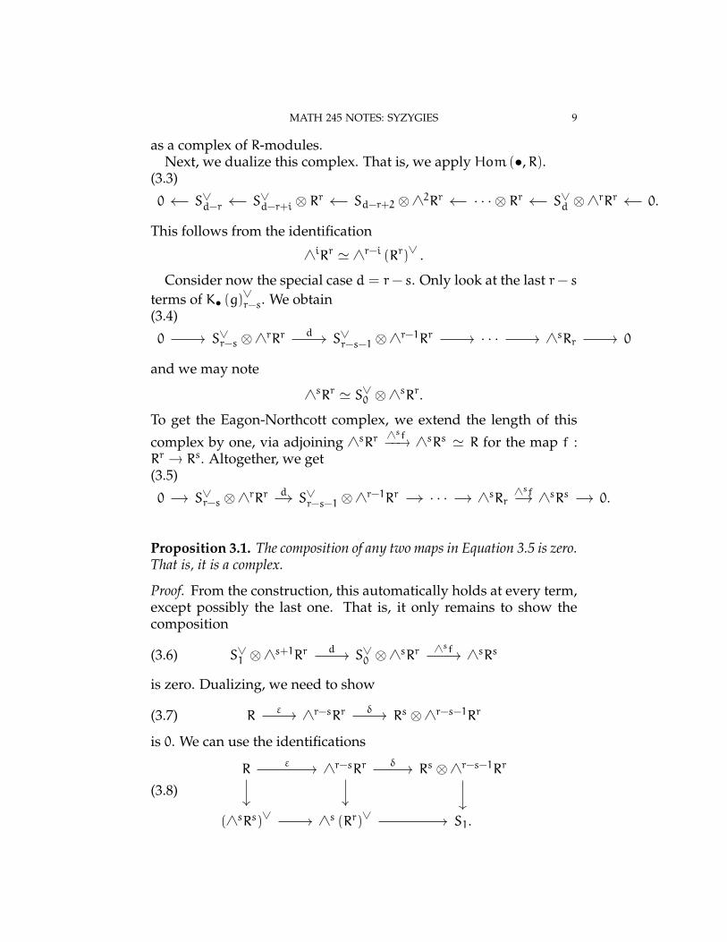
as a complex of R-modules.Next, we dualize this complex. That is, we apply Hom (•,R).
(3.3)
0 S∨d−r S∨d−r+i ⊗ Rr Sd−r+2 ⊗∧2Rr · · · ⊗ Rr S∨d ⊗∧rRr 0.
This follows from the identification
∧iRr ' ∧r−i (Rr)∨ .
Consider now the special case d = r− s. Only look at the last r− sterms of K• (g)∨r−s. We obtain(3.4)
0 S∨r−s ⊗∧rRr S∨r−s−1 ⊗∧r−1Rr · · · ∧sRr 0d
and we may note
∧sRr ' S∨0 ⊗∧sRr.
To get the Eagon-Northcott complex, we extend the length of this
complex by one, via adjoining ∧sRr∧sf−−→ ∧sRs ' R for the map f :
Rr → Rs. Altogether, we get(3.5)
0 S∨r−s ⊗∧rRr S∨r−s−1 ⊗∧r−1Rr · · · ∧sRr ∧sRs 0.d ∧sf
Proposition 3.1. The composition of any two maps in Equation 3.5 is zero.That is, it is a complex.
Proof. From the construction, this automatically holds at every term,except possibly the last one. That is, it only remains to show thecomposition
(3.6) S∨1 ⊗∧s+1Rr S∨0 ⊗∧sRr ∧sRsd ∧sf
is zero. Dualizing, we need to show
(3.7) R ∧r−sRr Rs ⊗∧r−s−1Rrε δ
is 0. We can use the identifications
(3.8)R ∧r−sRr Rs ⊗∧r−s−1Rr
(∧sRs)∨ ∧s (Rr)∨ S1.
ε δ
10 AARON LANDESMAN
This composition corresponds to an element of Hom(∧s+1Rr,Rs
).
Let e1, . . . , er be a basis for Rr. We have
δ ε(1)(ei1 ∧ · · ·∧ eis+1
)=∑
(−1)p+1 ε(1)(ei1 ∧ · · ·∧ eip ∧ · · ·∧ eis+1
)f(eip)
This is some element of Rs since∑(−1)p+1 ε(1)
(ei1 ∧ · · ·∧ eip ∧ · · ·∧ eis+1
)is an element of R. This follows from the definition. Then,
ε(1) ∈ Hom (∧sRr,R) ,
so
δ ε(1)(ei1 ∧ · · ·∧ eis+1
)=∑
(−1)p+1 ε(1)(ei1 ∧ · · ·∧ eip ∧ · · ·∧ eis+1
)f(eip)
=∑
(−1)p+1(f(ei1)∧ · · ·∧ f(eip)∧ · · ·∧ f
(eis+1
))· f(eip)
.
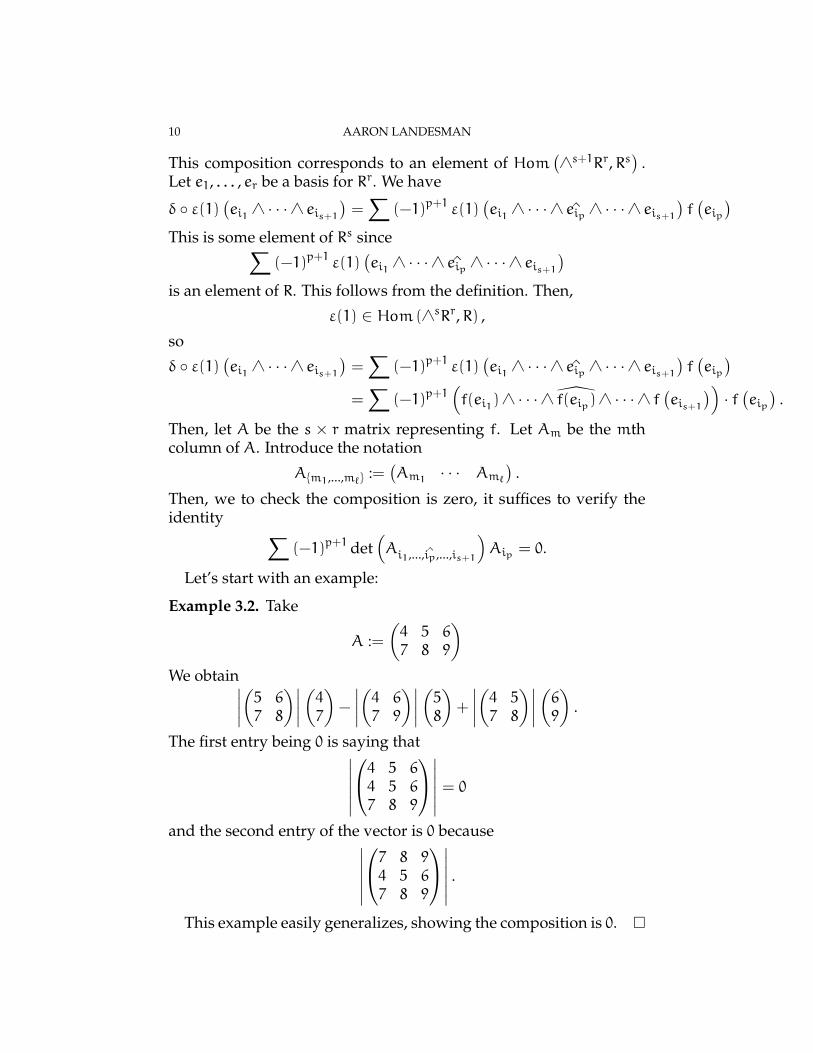
Then, let A be the s× r matrix representing f. Let Am be the mthcolumn of A. Introduce the notation
Am1,...,m` :=(Am1 · · · Am`
).
Then, we to check the composition is zero, it suffices to verify theidentity ∑
(−1)p+1 det(Ai1,...,ip,...,is+1
)Aip = 0.
Let’s start with an example:
Example 3.2. Take
A :=
(4 5 67 8 9
)We obtain∣∣∣∣(5 6
7 8
)∣∣∣∣ (47)−
∣∣∣∣(4 67 9
)∣∣∣∣ (58)+
∣∣∣∣(4 57 8
)∣∣∣∣ (69)
.
The first entry being 0 is saying that∣∣∣∣∣∣4 5 64 5 67 8 9
∣∣∣∣∣∣ = 0and the second entry of the vector is 0 because∣∣∣∣∣∣
7 8 94 5 67 8 9
∣∣∣∣∣∣ .
This example easily generalizes, showing the composition is 0.
MATH 245 NOTES: SYZYGIES 11
To recap, here is our definition:
Definition 3.3. Let f : Rr → Rs. The Eagon-Northcott complex is thecomplex(3.9)
0 R ∧sRr S∨1 ⊗∧s+1Rr · · · S∨r−s ⊗∧rRr 0∧sf d
and S = R [x1, . . . , xn] .
Remark 3.4. Next time we will find a criterion for the Eagon North-cott complex to be exact. The key to proving exactness will be theBuchsbaum-Eisenbud criterion for exactness.
Definition 3.5. Let ψ : Rr → Rs be a map of free R-modules. Wedefine
Ij(φ) ⊂ Rto be the ideal generated by the j× jminors.
Intrinsically, Ij(ψ) is the ideal given by the image of the map
∧jRr ⊗∧j(Rs)∨ → R.
This can be thought of as an element of
Hom(∧jRs,∧jRs
)given by ∧jφ. The rank of φ, notated rk(φ) is the greatest integer jso that Ij(φ) 6= 0. Then,
I (φ) := Irk(φ)(φ).
Proposition 3.6 (Proposition 20.8, Eisenbud’s commutative algebrabook). If φ : Rr → Rs is a morphism, then cokerφ is projective if and onlyif I(φ) = R. In this case, cokerφ has rank s− rkφ.
Proof. Omitted.
Next time, we’ll apply following criterion for exactness of a com-plex to the Eagon-Northcott complex.
Theorem 3.7 (Buchsbaum-Eisenbud). Let
(3.10) F0 F1 F2 · · · Fn 0f1 f2 fn
be a complex. Assume(1)
rk (Fk) = rk fk + rk fk+1and
12 AARON LANDESMAN
(2)
depth I(fk) ≥ k
for k = 1, . . . ,n.then F• is exact.
Proof. Omitted.
Definition 3.8. Recall that the depth of an ideal I is the maximallength of a regular sequence xi ∈ Rwith each xi ∈ I.
4. 4/12/17
Today’s goal is the Buchsbaum Eisenbud criterion for exactness.There are two main ingredients:
(1) Fitting ideals(2) The Peskine-Szpiro lemma
4.1. Fitting ideals. We’ll just state their definition and propertieswithout proof. Given a matrix
φ : Rr → Rs,
let the ideal Ijφ ⊂ R be the ideal generated by the j× jminors of φ.
Definition 4.1 (Fitting ideal). LetM be a finitely generated R-modulefor R noetherian (in the future we will assume R noetherian withoutcomment). Choose a presentation
(4.1) Ra Rb M 0.φ
Then,
Fitti(M) := Ib−i(φ).
Proposition 4.2. LetM be a finitely generated R-module. Then,(1) Fitti(M) is well defined (i.e., independent of choice of resolution)(2) Fitting ideals are functorial, meaning that for a maps of rings f :
R→ S, we have
Fittj (M⊗R S) = f(Fittj(M)) ⊂ S.
(3) As a consequence of the previous point, fitting ideals commute withlocalization.
Proof. Omitted.
MATH 245 NOTES: SYZYGIES 13
Remark 4.3. Recall that rkφ : F→ G is by definition
rkφ := maxi
j : Ij(φ) 6= 0
.
and
I(φ) := Irkφ(φ).
If M is a finitely generated R-module with presentation φ, we haveI(M) := I(φ).
Warning 4.4. I(φ) need not commute with localization because itmay be that rkφp < rkφ.
Remark 4.5. If we assume that I(φ) contains a nonzero divisor then
I(φ)p 6= 0for all p ∈ Spec R. This implies that rk(φp) ≥ rk(φ), which impliesrkφp = rkφ and so by Proposition 4.2
I(φ)p = I(φp).
Lemma 4.6. LetM be a finitely generated R-module. Then,M is projectiveof constant rank if and only if I(M) = R. In this case,
rk(M) = b− rkφ
for
φ : Ra → Rb
a presentation ofM.
Proof. See Eisenbud’s commutative algebra book.
4.2. The Buchsbaum Eisenbud criterion. Here is the setup for theBuchsbaum Eisenbud criterion for exactness.
We first recall some definitions:
Definition 4.7. Let M be a finitely generated R-module. A sequencef1, . . . , fr in R isM-regular if fi is a nonzero divisor onM forM/ (f1, . . . , fi−1)Mfor i = 1, . . . , r andM/ (f1, . . . , fr)M 6= 0.
Definition 4.8. Let I ⊂ R be an ideal. Then,
depthI(M) :=
maximal length of anM-regular sequence in I if IM 6=M∞ if IM =M.
If R is local then
depth(M) := depthm(M).
14 AARON LANDESMAN
Lemma 4.9. Let (R,m) be a local ring. Suppose
(4.2) 0 A B C 0
is a short exact sequence of finitely generated R-modules. Then,
(1)
depth(B) ≥ min (depthA, depthC) .
(2)
depth(C) ≥ min (depthB, depthA− 1)
(3)
depthA ≥ min (depthB, depthC+ 1) .
Proof. This follows from the characterization of depth in terms of Ext.(Recall depth(M) = mini Exti(k,M) 6= 0.)
Lemma 4.10 (Peskine-Szpiro). Let R be a local ring and let
(4.3) 0 Fn Fn−1 · · · F1 F0fn f1
be a complex with Fi a finitely generated R-module. Suppose
(1) depth(Fi) ≥ i and(2) depthHjF = 0 for j > 0.
Then, F• is exact.
Proof. Suppose F• is not exact. Let i > 0 be the largest i so that HiFis nonzero. If i = n, then
HnF ⊂ Fn.
But, depth(Fn) ≥ n > 0 by Lemma 4.9 applied to A = Hn(F),B =Fn,C = im fn.
So, we may assume i < n. Let i < n. As the complex is exact tothe left of Fi by induction. We then have a short exact sequence
(4.4) 0 im fj+1 Fj im fj 0
MATH 245 NOTES: SYZYGIES 15
using that for i < j ≤ n. From Lemma 4.9, we have
depth im Fj ≥ min(j, depth im fj+1 − 1
)≥ min
(j, depth im fj+2 − 2
)≥ min (j, depth (im fn) − (n− j)) .≥ min (j, depth (Fn) − (n− j)) .≥ min (j,n− (n− j)) .≥ j.
But, we also have the exact sequence
(4.5) 0 im fi+1 ker fi HiF 0.
By assumption, depthHiF = 0 but HiF 6= 0. Therefore,
depthHiF = 0
≥ min (depth ker fi, i)
This can only happen if depth ker fi = 0. Note that we have i > 0here. This contradicts that
ker fi ⊂ Fi
so
depth ker fi ≥ 1.
since depthFi ≥ i.
We now come to a useful criterion for the exactness of a complex.
Theorem 4.11 (Buchsbaum-Eisenbud). Let
(4.6) 0 Fn Fn−1 · · · F1 F0fn f1
be a complex of free finite R-modules. Suppose(1)
rkFi = rk fi + rk fi+1
(2) if I(fi) 6= R, then depth I(fi) ≥ i. for i ≥ 1.Then, F• is exact.
Remark 4.12. In fact, this is an if and only if statement, but we onlyneed one direction, so we only state and prove that direction.
16 AARON LANDESMAN
Proof. The second assumption guarantees I(fi) has a nonzero divisor.So, by Remark 4.5, we know the assumptions are preserved underlocalization. Therefore, we may assume R is local.
Let’s deal with exactness at Fi. That is, we want to show
(4.7) Fi+1 Fi Fi−1fi+1 fi
is exact.We first consider the case i > d := depthR, we have
I(fi+1) = I(fi) = R,
by the second assumption.By Lemma 4.6, we have cokerFi is free of rank
rk cokerFi = rkFi − rk fi+1.
Construct
(4.8) Fi cokerFi Fi−1.fi
To proving exactness at Fi, it suffices to show fi is injective. We seethat
rk fi = rk fi= rkFi − rk fi+1= rk cokerFi
We hence have
I(fi) = I(fi) = R.
Then, dualizing the sequence
I(f∨i
)= R.
By Lemma 4.6 we have cokerfi∨
is free of rank
rk cokerFi − rk fi∨= rk fi= 0.
This implies fi∨
is surjective so fi is injective.To conclude, we only need prove the case that i ≤ d. In this case,
we will apply Lemma 4.10. By truncating F•, and replacing Fd withcokerfd+1, we may assume that F• has length at most d. That is, wemay assume n ≤ d.
Without generality, we have that R is local.
MATH 245 NOTES: SYZYGIES 17
Lemma 4.13. Suppose F• satisfies the following condition: (F•)p is exactfor every p 6= m in the local ring (R,m).
Proof. By this hypothesis, we have
Supp (HiF•) ⊂ m .
Therefore, there is some ` for which m`HiF• = 0. That is,
depthHiF = 0.
Note that each Fi is free, so depthFi = d ≥ i. Therefore, by Lemma 4.10,we know F• is exact.
To complete the proof, it suffices to reduce to the case that (F•)p isexact for every p 6= m.
In the general case, we induct on dimR. If dimR = 0, then weare done as there are no primes other than m. If dimR = n+ 1 thendimRp < dimR. Therefore, by the induction hypothesis for the ringRp, which is of lower dimension, we know that (F•)p has vanishingcohomology, and therefore the same follows for F• by Lemma 4.13.
5. 4/14/17
We’ll now discuss some applications of the Buchsbaum-Eisenbudcriterion for exactness of a complex in a geometric setting. In par-ticular, we’ll examine the relation to the Eagon-Northcott complex.Let f : Rr → Rs for r ≥ s. Recall we constructed an Eagon-Northcottcomplex associated to f Eagon-Northcott(f) from the complex(5.1)
0 R ∧sRr S∨ ⊗∧s+1Rr S∨2 ⊗∧s+2Rr · · · S∨r−s ∧r Rr 0
∧sf d
where we are using that R ' ∧sRs and S = R[x1, . . . , xs].We state the following theorem without proof, though we will
come back to it in Corollary 6.3.
Theorem 5.1 (Eagon-Northcott). Assume depth Is(f) ≥ r+1− s. Then,Eagon-Northcott(f) is exact.
5.1. Rational normal curves. Recall a rational normal curve C ⊂ Pd
is the embedding from P1φL−−→ Pd for L = OP1(d). Recall that C is
smooth, rational, degree d, nondegenerate, The ideal of C is gen-erated by the equations xixj − xi−1xj+1. It’s clear that the rationalnormal curves lies in the intersection of these equations, and you
18 AARON LANDESMAN
can check it actually is the vanishing of these equations by comput-ing the Hilbert polynomial (in fact, these equations already form aGrobner basis, so you can just use the leading terms).
Let
A =
(x0 · · · xd−1x1 · · · xd
)be a 2× dmatrix of linear form. Let IC be the ideal generated by the2× 2 minors of A. Let R = C [x0, . . . , xd] (be the graded ring). ViewA as a map f : Rd(−1) → R2. Let IC = I2(f) as C has codimensiond− 1.
As C has codimension d− 1, we have depth I2(f) = d− 1. There-fore, by Theorem 5.1, Eagon-Northcott(f) is exact.
Let S = R[y1,y2]. Recall that Eagon-Northcott(f) is the complex(5.2)
R ∧2Rd(−2)(R2)∨ ⊗∧3Rd(−3)
(Sym2 R2)∨ ⊗∧4Rd(−4) · · · (Symd−2 R
2)∨ ⊗∧dRd(−d) 0
∧2f
using that S∨1 ' R2 by identifying y1,y2 with the basis of R2 andidentifying S2 ' Sym2 R
2. Note that we have an exact complex
(5.3) 0 R/IC Eagon-Northcott(f)
Let S = k [x0, . . . , xn]. Recall that a graded free exact S-complex(F•,d•) is minimal if each di takes a basis of Fi to a minimal set ofgenerators of im di.
Proposition 5.2. Let F• be a graded free exact complex. Then F• is minimalif and only if im di is contained in (x0, . . . , xn) Fi−1.
Proof. The proof uses the graded Nakayama lemma. We recall itnow:
Lemma 5.3 (Graded Nakayama lemma). Suppose M is a finitely gen-erated graded S-module. Let m = (x0, . . . , xn). If a1, . . . ,ar generateM/mM. Then a1, . . . ,ar ∈ m generateM.
Proof. The idea is to look for elements of least degree inM/ (a1, . . . ,ar).
Exercise 5.4. Flush this idea out to give a proof.
MATH 245 NOTES: SYZYGIES 19
By the graded Nakayama lemma, we know that F• is minimal, ifand only if
Fi/mFidi−→ im di/mim di.
is an isomorphism. Note that we have an exact sequence
(5.4) Fi+1 Fi im di 0
The statement that di above defines an isomorphism is equivalent tothe map di+1
Fi+1/mFi+1di+1−−−→ Fi/mFi
is 0. That is, im di+1 ⊂ (x0, . . . , xd) Fi.
If Sa(c) f−→ Sb(c+ 1) is a morphism then f is represented by a ma-trix of linear forms.
Corollary 5.5. We have that Eagon-Northcott(f) is minimal.
Proof. This is just because at each step we are multiplying by linearforms, so the result follows from Proposition 5.2.
6. 4/19/17
We want to find the syzygies of a k gonal curve, meaning a curveC with a map f : C → P1. Let A := f∗OP1(1). We have a scroll XAwith C ⊂ XA ⊂ Pg−1 and a map
H0(A)⊗H0(ωC ⊗A∨)→ H0(ωC).
We also have a map PEf(−2)→ P1. We have an exact sequence
(6.1) Ef f∗ωf O1P.
Let H be a hyperplane class and let R be the ruling in the scroll. Wehave
h0(C,A) ' h0 (P (Ef(−2)) ,R)
and
H0(C,ωC ⊗A∨
)' H0 (P (Ef (−2)) ,H− R) .
20 AARON LANDESMAN
We also have a map
(6.2)C P (Ef (−2))
Pg−1.
We have that
j (P (Ef (−2))) ⊂ XA.
Recall that H0(C,A2
)= 3, meaning j is an embedding.
Proposition 6.1. We have P (Ef (−2)) ' XA.
Proof. Recall that XA was defined so that u, v is a basis of H0(C,A)and t1, . . . , t` are a basis of H0(ωC −A), with ` = g+ 1− k.
We have that IXA is generated by the 2× 2minors of
M :=
(ψut1 · · · ψut`ψrt1 · · · ψrt`
)with ψuti ∈ H0(Pg−1,O(1)) ' H0(C,ωC). It suffices to show XA isirreducible of dimension b− 1 = dim P (Ef (−2)).
Let
V := im(H0(A)⊗H0(ωC −A)→ H0(C,ωC)
).
We have PV∨ ⊂ Pg−1 with H0(PV∨,O(1)) ' V . Then, XA is a coneover the projective variety PV∨ ' Pr defined by the 2× 2minors ofMPV∨ .
To prove XA is irreducible of codimension g− k = `− 1, we mayassume the multiplication map
V ' H0(Pg−1,O(1)),since a cone over a variety is irreducible of codimension d if and onlyif the variety is irreducible of codimension d.
Then,M defines a morphism of projective bundles
ψ : Og+1−k(−1)→ O2,
and XA is the degeneracy locus of ψ. That is, XA is the locus whereψ does not have full rank. Restricting
ψ|XA : Og+1−k(−1)→ O2
has rank at most 1. Since the multiplication map
H0(A)⊗H0(ωC −A)→ H0(C,ωC)
MATH 245 NOTES: SYZYGIES 21
is surjective, so V ' H0(Pg−1,O(1)), it is not possible for all entriesofM to vanish.
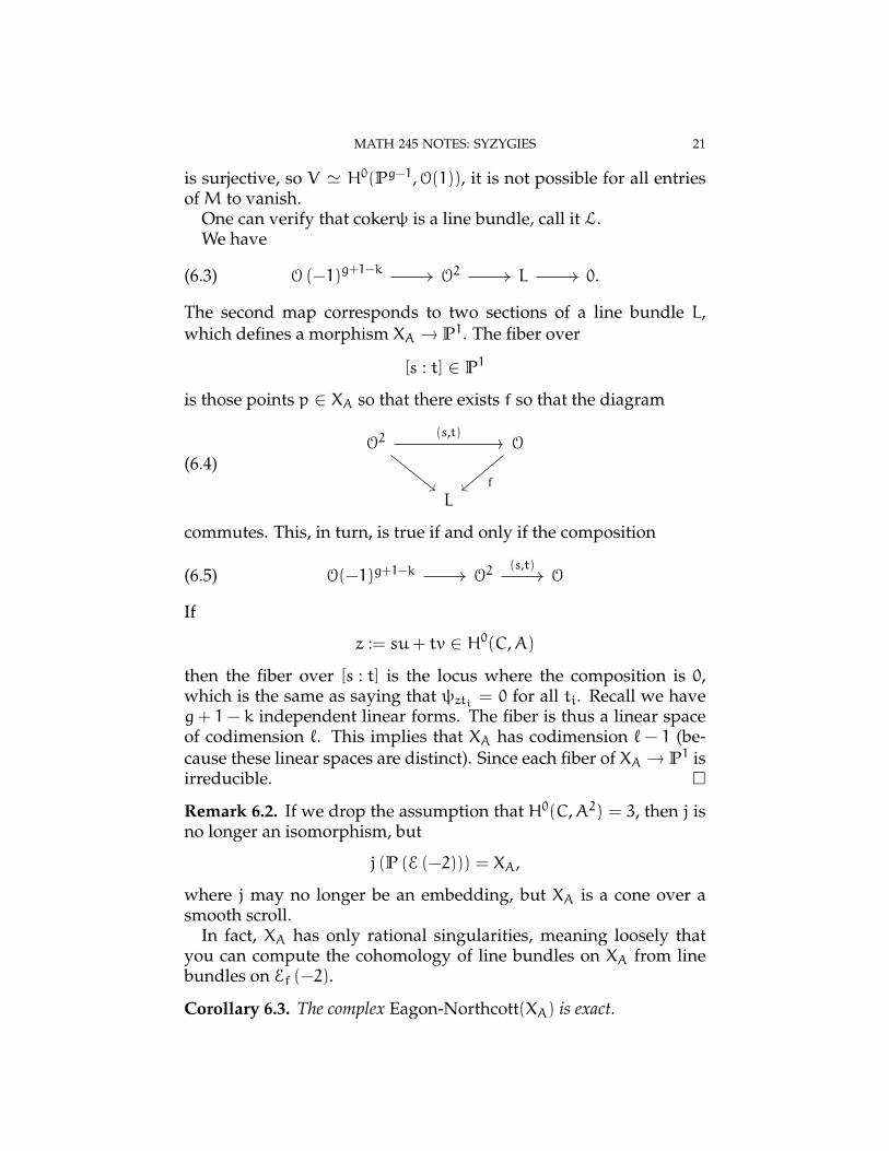
One can verify that cokerψ is a line bundle, call it L.We have
(6.3) O (−1)g+1−k O2 L 0.
The second map corresponds to two sections of a line bundle L,which defines a morphism XA → P1. The fiber over
[s : t] ∈ P1
is those points p ∈ XA so that there exists f so that the diagram
(6.4)O2 O
L
(s,t)
f
commutes. This, in turn, is true if and only if the composition
(6.5) O(−1)g+1−k O2 O(s,t)
If
z := su+ tv ∈ H0(C,A)
then the fiber over [s : t] is the locus where the composition is 0,which is the same as saying that ψzti = 0 for all ti. Recall we haveg+ 1− k independent linear forms. The fiber is thus a linear spaceof codimension `. This implies that XA has codimension ` − 1 (be-cause these linear spaces are distinct). Since each fiber of XA → P1 isirreducible.
Remark 6.2. If we drop the assumption that H0(C,A2) = 3, then j isno longer an isomorphism, but
j (P (E (−2))) = XA,
where j may no longer be an embedding, but XA is a cone over asmooth scroll.
In fact, XA has only rational singularities, meaning loosely thatyou can compute the cohomology of line bundles on XA from linebundles on Ef (−2).
Corollary 6.3. The complex Eagon-Northcott(XA) is exact.
22 AARON LANDESMAN
We have
bi,j(OXA
)=
1 if i = j = 0i ·(g+1−ki+1
)if j = 1, i > 0
0 else
For a projective variety Z, define
`(Z) := minm : bp,1(OZ) = 0,p > m
.
called the length of the 2-linear strand. For brevity, we will just callthis the length of the linear strand.
Conjecture 6.4 (Green). Suppose C has gonality k and Cliff(C) =k− 2. Then,
φωC : C→ Pg−1
for A ∈W1k. Then,
` (ΓC(ωC)) = `(OXA
)= g− k.
There is a refinement of this due to Schreyer.
Conjecture 6.5 (Schreyer). If W1k is a reduced point A and A is the
unique line bundle line bundle of degree at most k− 1with CliffC =k− 2, then
bg−k,1 (C,ωC) = bg−k,1 (XA,O(1)) = g− k.
6.1. Picard group of Mg.
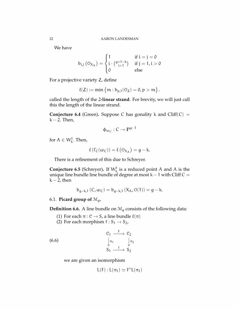
Definition 6.6. A line bundle on Mg consists of the following data:
(1) For each π : C→ S, a line bundle `(π)(2) For each morphism f : S1 → S2,
(6.6)C1 C2
S1 S2
π1
F
π2
f
we are given an isomorphism
L(F) : L(π1) ' F∗L(π1)
MATH 245 NOTES: SYZYGIES 23
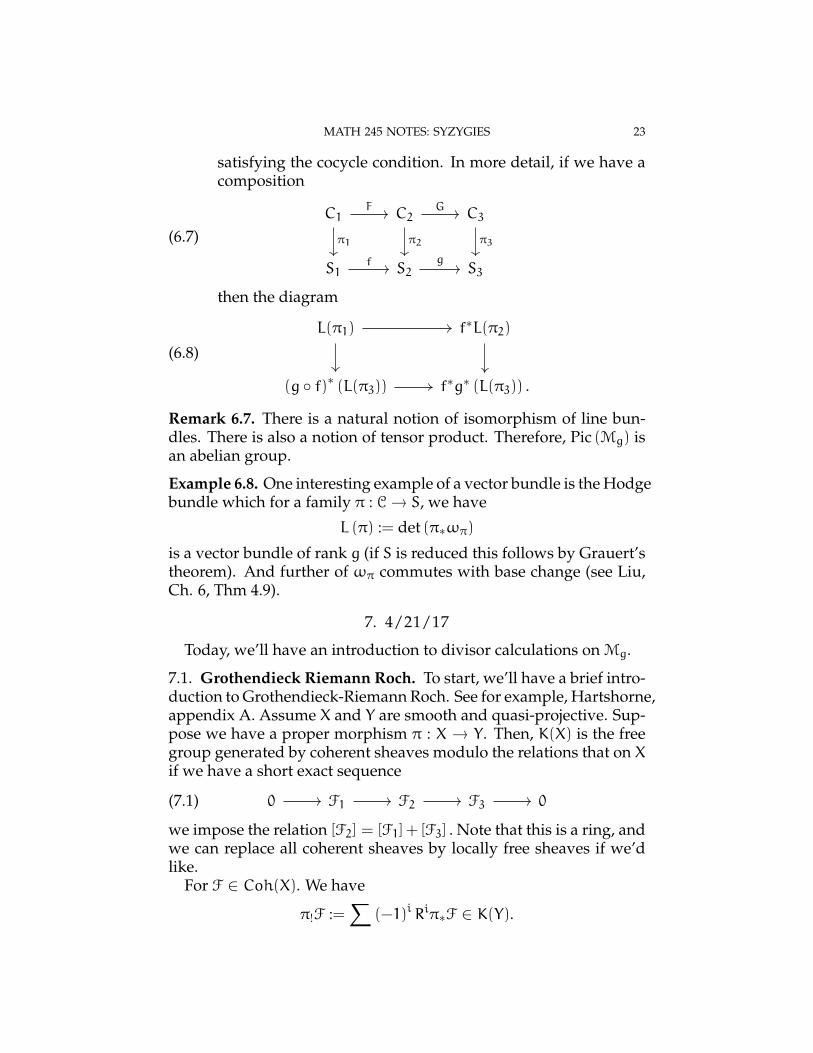
satisfying the cocycle condition. In more detail, if we have acomposition
(6.7)C1 C2 C3
S1 S2 S3
F
π1
G
π2 π3
f g
then the diagram
(6.8)
L(π1) f∗L(π2)
(g f)∗ (L(π3)) f∗g∗ (L(π3)) .
Remark 6.7. There is a natural notion of isomorphism of line bun-dles. There is also a notion of tensor product. Therefore, Pic (Mg) isan abelian group.
Example 6.8. One interesting example of a vector bundle is the Hodgebundle which for a family π : C→ S, we have
L (π) := det (π∗ωπ)
is a vector bundle of rank g (if S is reduced this follows by Grauert’stheorem). And further of ωπ commutes with base change (see Liu,Ch. 6, Thm 4.9).
7. 4/21/17
Today, we’ll have an introduction to divisor calculations on Mg.
7.1. Grothendieck Riemann Roch. To start, we’ll have a brief intro-duction to Grothendieck-Riemann Roch. See for example, Hartshorne,appendix A. Assume X and Y are smooth and quasi-projective. Sup-pose we have a proper morphism π : X → Y. Then, K(X) is the freegroup generated by coherent sheaves modulo the relations that on Xif we have a short exact sequence
(7.1) 0 F1 F2 F3 0
we impose the relation [F2] = [F1] + [F3] . Note that this is a ring, andwe can replace all coherent sheaves by locally free sheaves if we’dlike.
For F ∈ Coh(X). We have
π!F :=∑
(−1)i Riπ∗F ∈ K(Y).
24 AARON LANDESMAN
Definition 7.1. For E a vector bundle, we define the total Chern class
ct(E) :=∑i
ci (E) ti
with
ci(E) ∈ A∗ (X, Q) .
the Chern class.
Remark 7.2. By the splitting principle, we can write
ct(E) :=∑i
ci (E) ti
=∏i
(1+αit) .
Definition 7.3. If E is a vector bundle with ct(E) =∏
(1+αit), thenthe Chern character
Ch (E) =∑i
eαi
Example 7.4. Viewing Ch (E) as an element of the graded ring Chi(E)is the ith graded piece of Ch (E). We have
Ch0 (E) = rkECh1(E) = c1(E).
We have
Ch2 (E) =c21−2 c22
.
Lemma 7.5. The Chern class defines a ring homomorphism
K(X)→ A∗(X)
F 7→ Ch(F).
Proof.
Exercise 7.6. Verify this.
Definition 7.7. Let E be a vector bundle with ct(E) =∏i (1+αit).
We define the Todd class
Td (E) :=∏i
αi1− e−αi
.
MATH 245 NOTES: SYZYGIES 25
Remark 7.8. The Todd class is multiplicative, so that if we have
(7.2) 0 F1 F2 F3 0
then
Td (F2) = Td (F1)Td (F3)
Theorem 7.9 (Grothendieck Riemann Roch). Suppose π : X → Y isproper. Then,
Chπ!F = π∗ (cF Td(Tπ))
Let F ∈ K(X). where Tπ = TX − π∗TY .
Theorem 7.10 (Mumford’s formula). Let π : C → Mg be the universalcurve. Let
λ := c1 (π∗ωπ)
be the hodge class and
κ := π∗ (c1ωπ · c1ωπ)be the kappa class. Then,
κ = 12λ.
Proof. We have
π!ωπ = π∗ωπ − R1π∗ωπ
= π∗ωπ − (π∗OC)∨
= π∗ωπ −O∨Mg
= π∗ωπ +OMg
This implies
Ch (π!ωπ) = Ch (π∗ωπ) + Ch(OMg
)= Ch (π∗ωπ) + 1
= g+ 1+ c1(π∗ωπ) +1
2
(c21 (π∗ωπ) − c2 (π∗ωπ)
)+ · · ·
Using that Tπ = −ωπ, we have
π∗ (Ch (ωπ)Td Tπ)
= π∗
(1+ c1 (ωπ) +
1
2
(c21 − c2
)+ · · ·
)(1−
1
2c1 (ωπ) +
1
12c1 (ωπ)
2 + · · ·)
.
26 AARON LANDESMAN
We then have
λ = [Ch (π!ωπ)]1 ,
so
π∗ (Ch (ωπ)Td (−ωπ)) = π∗
(1+
1
2c1(ωπ) +
1
2c21 −
1
2c21 +
1
12c21
).
We obtain
[π∗ (Ch (ωπ)Td (−ωπ))]1 =1
12κ.
7.2. Hurwitz Divisor.
Definition 7.11. Assume that g = 2k− 1 is odd. Define the Hurwitzdivisor Hur ⊂Mg to be
C : ∃f : C→ P1 of degree at most k
.
Remark 7.12. We can also define Hur ⊂ Mg determinantally. Con-sider π : C→Mg. Define
Cn := C×Mg · · · ×Mg C
as an n-fold fiber product. Let pi : Cn → C be the ith projection.Consider πn : Cn →Mg. Consider
Z =
(p1, . . . ,pk) ∈ Ck : h0
(C,∑i
pi
)≥ 2
.
Then, π(Z) is Hur.
Remark 7.13. Note that π is not finite onZ, since the fibers are at least1 dimensional as the divisor moves by the assumption h0(C,
∑i pi) >
1.
Warning 7.14. Therefore, π|Z has fibers of dimension at least 1, mean-ing π∗ (Z) = 0. Here is a fix to the issue that π is not generically finite,so the pushforward would be 0 by definition.
We can fix this by demanding that the first point p1 lies in somefixed canonical divisor. That is, we define
Ki ∈ Pic(Ck):= p∗1 (ωπ) .
Then, we can define
Hur :=1
(2g− 2) (k− 1) !· (πk)∗ ([K1] · [Z]) .
MATH 245 NOTES: SYZYGIES 27
We are almost ready to define [Z] determinantally.
Definition 7.15. Define the diagonal
∆i,j ⊂ Cn
to be the (i, j)th diagonal, i.e., the image of Cn−1 → Cn under the mapsending p1, . . . ,pn−1 to p1, . . . ,pi,pi+1, . . . ,pj−1,pi,pj+1, . . . ,pn−1.
Given the short exact sequence(7.3)
0 OCk+1 OCk+1
(∑j∆j,k+1
)O∑
i ∆j,k+10
and let
p : Ck+1 → Ck
be the projection away from the last factor.
Remark 7.16. Note that
p∗
OCk+1
k∑j=1
∆j,k+1)
' OCk+1 .
If (p1, . . . ,pk) ∈ Ck are general, then h0(C,∑i pi) = 1.
This is the same as saying the map
H0(C,OC) ' H0(OC
(∑i
pi
))for p1, . . . ,pk general on C. We have a natural map
p∗ (OCk+1)→ p∗(OCk+1
(∑∆j,k+1
)).
The above computation implies that for any sufficiently small openU, the map
p∗OCk+1(U)→ p∗
OCk+1
∑j
∆j,k+1
(U) .
Taking derived pushforwards of the exact sequence(7.4)
0 OCk+1 OCk+1
(∑j∆j,k+1
)O∑
i ∆j,k+10
28 AARON LANDESMAN
on 0th degree, we get
p∗OCk+1 ' p∗OCk+1
∑j
∆j,k+1
and continuing we get
(7.5)
0 p∗O∑i ∆j,k+1
R1p∗OCk+1 R1p∗OCk+1
(∑j∆j,k+1
)0
α
Note that the first term p∗O∑i ∆j,k+1
is locally free of rank 1, and thenZ is the locus where the map α is not injective.
8. 4/24/17
Last time, we were discussing the divisor Hur ⊂ Mg for g = 2k−1. We were discussing the construction of the Hurwitz divisor asπk : Ck →Mg, with
Hur :=1
(2g− 2) (k− 1) !πk∗ ([Z]K1)
where K1 is the pullback of the canonical divisor of C → Mg alongthe first projection Ck → C. Let’s review how this went. We can view
[Z] =(p1, . . . ,pk) : h0(C,
∑pi) ≥ 2
.
We have an exact sequence(8.1)
0 OCk+1 O (∑∆i,k+1) O∑
∆i,k+10
Pushing this forward along p : Ck+1 → Ck, which is projection ontothe first k factors, we get an isomorphism between the pushforwardof the first two sheaves, we get a short exact sequence(8.2)
0 p∗O∑∆i,k+1
R1p∗OCk+1 R1p∗ (O∑∆i,k+1) 0
α
The fibers αq (for q corresponding to a curve) are given by(8.3)
0 H0(OC) H0(OC (∑pi)) H0
(O∑
i pi
)H1(OC)
αq
and αq fails to be injective if and only if h0 (OC (∑pi)) ≥ 2. We will
define Z as the locus of points qwith αq not injective.
MATH 245 NOTES: SYZYGIES 29
Theorem 8.1 (Porteous). Suppose X is a smooth scheme over C and φ :E→ F is a map of vector bundles with E of rank n and F a vector bundle ofrankm. Let
Xk(φ) := p ∈ X : φp has rank at most k .
Assume Xk(φ) has the expected dimension (m− k) (n− k). Then,
[Xk (φ)] = ∆m−k,n−k (c+(F)/ ct(E)) .,
where ∆(•) is defined as follows. If
a(t) =∑k
aktk
is a formal power series, we have
∆p,q(a(t)) := det
qp · · · ap+q−1...
. . ....
ap−q+1 · · · ap.
To apply Porteous’ theorem, we must know that Z ⊂ Ck has codi-
mension g− (k− 1) = k. For this, we need the following:Clebsch The Hurwitz stack
Hd,g :=C→ P1 : degd,C smooth of genus g
/ Aut
(P1)
.
has dimension 2g− 5− 2d.Segre The map Hd,g → Mg is generically finite for (with some as-
sumption on g and d that Michael wasn’t exactly sure about,he thought it was g ≥ 7).
Exercise 8.2. Show that the above results mean we can apply Porte-ous’ theorem to show Hur is indeed a divisor.
Theorem 8.3 (Harris-Mumford, Harer, Kempf). We have(1)
[Hur] = cλ
(2) In fact,
c =(2k− 4) !
k! (k− 2) !.
Remark 8.4. Harris-Mumford used test curves, explicit curves in Mg
that they understood well for which they could compute things ex-plicitly.
30 AARON LANDESMAN
Proof. We have
[Z] = ∆g−k+1,1
(ct
(R1p∗
(OC
(∑∆j,k+1
))))= cg−k+1
(R1p∗
(OC
(∑∆j,k+1
)))= 1− p!
(OC
(∑∆j,k+1
)).
The Chern classes are expressible as polynomials in Chd. That is, [Z]is polynomial in
Ch(p!
(OC
(∑∆j,k+1
)))= p∗
(Ch(OC
(∑∆i,k+1
)Td (ωp)
)),
using, Grothendieck Riemann-Roch. Therefore, [Z] is a polynomialin
p∗([∆j,k+1
])
and
p∗ [ωp] = p∗(Kk+1).
where Ki = p∗iωC/Mg with pi the ith projection Cn → C. To simplifythis, we can use the push-pull formula. We have
p∗([∆j,k+1 · p∗ (ζ)
])= p∗
([∆j,k+1
])· ζ
= ζ
Note here p∗ζ ∈ A∗(Ck). We want to express as much of the above
as possible as the pullback of cycles on Ck. We have
[∆i,k+1] · · ·[∆j,k+1
]= [∆i,k+1] · p∗
[∆i,j]
.
Loosely this is saying that if p1, . . . ,pk+1 with pi = pk+1 and pj =pj+1 this is equivalent to saying pi = pk+1 and pi = pj. We also havethe relation [
∆j,k+1]· Kk+1 = [∆i,k+1] · p∗Kj.
The above relations let us deal with any monomial in which norepeated
[∆j,k+1
]appears. For example,
p∗ (∆1,k+1 ·∆2,k+1 ·∆3,k+1 · Kk+1) = p∗ (∆1,k+1p∗∆1,2p∗∆1,3p∗K1)= ∆1,2 ·∆1,3 · · ·K1.
Next, we have to deal with powers of these diagonals. For this, weuse the self intersection formula (see Hartshorne, p. 431).
Lemma 8.5 (Self Intersection Formula). Suppose we have a closed im-mersion of schemes (or stacks) i : Y → X with both smooth of codimensionr. We have Y · Y = i∗ (cr (NY/X)).
MATH 245 NOTES: SYZYGIES 31
Using this self intersection formula, and letting q : Ck+1 → Ck beprojection away from the jth factor, we get[
∆j,k+1]2
= i∗(
c1(N∆j,k+1/Ck+1
))= −i∗ c1 (Ωq)
= −[∆j,k+1
]p∗(Kj)
.
We then conclude that [Z] can be written as a polynomial in thecycles ∆i,j and Ki. We also may include p∗
(K`k+1
)for some positive
integer e. To simplify this, we use flat pullback of cycles
Lemma 8.6 (Flat pullback, Fulton proposition 1.7). Suppose we have aCartesian square
(8.4)A B
C D
f
i g
h
with f flat and g proper, we have
c∗f∗α = h∗g∗α
for α ∈ A∗(B).
In our situation, we can apply this to the diagram
(8.5)Ck+1 C
Ck Mg
pk+1
p π
πk
we obtain
p∗(K`k+1
)= π∗kπ∗
(K`)
Therefore, Hur is a polynomial in πk,∗ times polynomials in ∆k,j,Kj’s and π∗kπ∗
(K`). To conclude, one can factor πk as a composition
Ck → Ck−1 → · · ·→ C.
Repeating the above, things remain polynomials in the analogousclasses, except that certain ∆i,j classes become 1. When one factorsthis, one obtains that [Hur] is a polynomial in π∗
(K`). Note that Hur
32 AARON LANDESMAN
is a divisor, and the only divisor in π∗(K`) is π∗(K2) (meaning ` = 1).This implies by dimension reasons that
Hur = cπ∗(K2)= κ,
so Hur = c ′λ, which is Mumford’s formula.
9. 4/26/17
9.1. Graded Tor. Today, we’ll discuss graded tor. Let R be a gradedk-algebra. LetM andN be two graded R-modules. Note thatM⊗kNis graded. We have
(M⊗RN)d =
∑i
mi ⊗ ni : deg(mi) + deg(ni) = d
.
Note that TorR(M,N) is a bigraded module gotten by taking a pro-jective resolution
(9.1) 0 M P0 P1 · · ·f0 f1
Then, tensoring up, we obtain a complex of graded R-modules P•⊗RN. Then,
Torpk(M,N)q
is the pth homology of (P• ⊗RN)q. Then,
TorpR(M,N) = ⊕q≥0Torp(M,N)q.
We have
Torp(M,N)q ' Torp(N,M)q.
9.2. The Koszul complex, revisited. Let S = k [x0, . . . , xn] andM bea finitely generated S-module. We have a minimal free resolution
(9.2) 0 M F0 · · · Fn+1
We know that for a minimal free resolution, if we tensor by k :=S/ (x0, . . . , xn), all differentials are 0, and therefore, all differentialsare 0 by Nakayama’s lemma. That is, if we have Fi = ⊕jS(−i− j)bi,j .Therefore,
Fi ×S k = ⊕jk(−i− j)bi,j(9.3)
as a graded k-module. We then have
dim(ToriR(M,k)i+j
)= bi,j(M).
MATH 245 NOTES: SYZYGIES 33
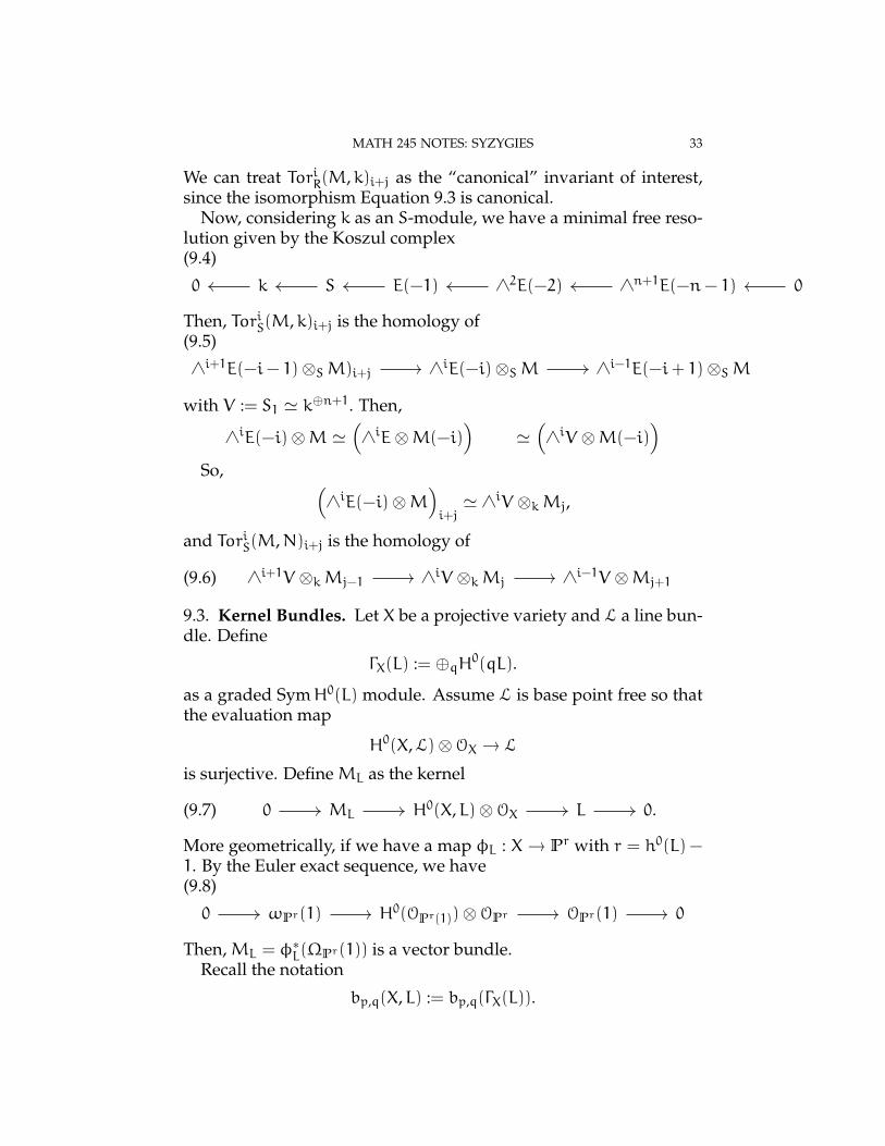
We can treat ToriR(M,k)i+j as the “canonical” invariant of interest,since the isomorphism Equation 9.3 is canonical.
Now, considering k as an S-module, we have a minimal free reso-lution given by the Koszul complex(9.4)
0 k S E(−1) ∧2E(−2) ∧n+1E(−n− 1) 0
Then, ToriS(M,k)i+j is the homology of(9.5)
∧i+1E(−i− 1)⊗SM)i+j ∧iE(−i)⊗SM ∧i−1E(−i+ 1)⊗SM
with V := S1 ' k⊕n+1. Then,
∧iE(−i)⊗M '(∧iE⊗M(−i)
)'(∧iV ⊗M(−i)
)So, (
∧iE(−i)⊗M)i+j' ∧iV ⊗kMj,
and ToriS(M,N)i+j is the homology of
(9.6) ∧i+1V ⊗kMj−1 ∧iV ⊗kMj ∧i−1V ⊗Mj+1
9.3. Kernel Bundles. Let X be a projective variety and L a line bun-dle. Define
ΓX(L) := ⊕qH0(qL).
as a graded SymH0(L) module. Assume L is base point free so thatthe evaluation map
H0(X,L)⊗OX → L
is surjective. DefineML as the kernel
(9.7) 0 ML H0(X,L)⊗OX L 0.
More geometrically, if we have a map φL : X → Pr with r = h0(L) −1. By the Euler exact sequence, we have(9.8)
0 ωPr(1) H0(OPr(1))⊗OPr OPr(1) 0
Then,ML = φ∗L(ΩPr(1)) is a vector bundle.
Recall the notation
bp,q(X,L) := bp,q(ΓX(L)).
34 AARON LANDESMAN
We have a short exact sequence(9.9)
0 ∧p+1ML ⊗ (q− 1)L ∧p+1H0(L)⊗ (q− 1)L ∧pML ⊗ qL 0
(see Hartshorne, II-5).Taking global sections, we get a map
∧p+1H0(L)⊗H0 ((q− 1)L) α−→ H0 (∧pML ⊗ qL) .
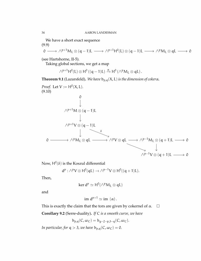
Theorem 9.1 (Lazarsfeld). We have bp,q(X,L) is the dimension of cokerα.
Proof. Let V := H0(X,L).(9.10)
0
∧p+1M⊗ (q− 1)L
∧p+1V ⊗ (q− 1)L
0 ∧pML ⊗ qL ∧pV ⊗ qL ∧p−1ML ⊗ (q+ 1)L 0
∧p−1V ⊗ (q+ 1)L 0
δ
Now, H0(δ) is the Koszul differential
dp : ∧pV ⊗H0(qL)→ ∧p−1V ⊗H0((q+ 1)L).
Then,
kerdp ' H0(∧pML ⊗ qL)
and
im dp+1 ' im (α) .
This is exactly the claim that the tors are given by cokernel of α.
Corollary 9.2 (Serre-duality). If C is a smooth curve, we have
bp,q(C,ωC) = bg−2−p,3−q(C,ωC).
In particular, for q > 3, we have bp,q(C,ωC) = 0.
MATH 245 NOTES: SYZYGIES 35
Proof. Consider
∧p+1V ⊗H0((q− 1)L) α−→ H0(∧pML ⊗ qL).We get an exact sequence(9.11)
0 ∧p+1ML ⊗ (q− 1)L ∧p+1V ⊗ (q− 1)L ∧pML ⊗ qL 0.
Observe ∧pV∨ ' ∧r−pV ⊗ detV∨. Then,
∧p+1V ⊗H0((q− 1)ωC)∨ ' ∧g−p−1V ⊗H1 ((2− q)ωC) .
We also have
H0(∧pML ⊗ qωC)∨ ' H1(∧pM∨L ⊗ (1− q)ωC).
We have rkML = k − 1, so detML ' L, as comes from the exactsequence. Therefore,
H0(∧pML ⊗ qωC)∨ ' H1(∧pM∨L ⊗ (1− q)ωC)
' H1(∧g−1−pMωC ⊗ (2− q)ωC).
Then,
cokerα∨ = ker(H1(∧g−1−pMωC ⊗ (2− q)ωC
)→ ∧g−p−1V ⊗H1 ((2− q)ωC))
.
Using the long exact sequence Equation 9.11, we have
cokerα∨ = ker(H1(∧g−1−pMωC ⊗ (2− q)ωC
)→ ∧g−p−1V ⊗H1 ((2− q)ωC))
.
' coker(∧g−1−pH0(ωC)⊗H0 ((2− q)ωC)→ H0
(∧g−2−pM∧C ⊗ (3− q)ωC
)).
The first term has dimension bg−2−p,3−q(C,ωC). This finishes theproof by Theorem 9.1.
10. 4/28/17
Let S = k [x1, . . . , xn]. Given an exact sequence of graded S-modules
(10.1) 0 M1 M2 M3 0
we get a long exact sequence on tor(10.2)
· · · Tori+1S (M3,k) ToriS(M1,k) Tori(M2,k) · · ·
Taking the i+ jth strand of this complex, we get(10.3)
· · · Tori+1S (M3,k)i+j ToriS(M1,k)i+j Tori(M2,k)i+j · · ·
36 AARON LANDESMAN
We define
Ki,j(M) := ToriS(M,k)i+jso
bi,j(M) = dimk Ki,j(M).
Definition 10.1. The long exact sequence of Koszul cohomology isthe exact sequence obtained above, which can be rewritten as(10.4)· · · Ki+1,j−1(M3) Ki,j(M1) Ki,j(M2)
Ki,j(M3) Ki−1,j+1(M3) · · ·
Lemma 10.2 (Semicontinuity). Suppose π : X→ S is a flat map of finitetype schemes over Spec C (where S is not a polynomial ring). Suppose S isintegral and L ∈ Pic(X). Assume
h0(Xs,Ls),h0(Xs, (q− 1)Ls),h0(Xs,qLs),h0(Xs, (q+ 1)Ls)
are all constant for closed points s of S. Then, the function
ψ : S→ Z
s 7→ bp,q(Xs,Ls) = bp,q(ΓLs(X))
is upper semicontinuous.
Proof. Without loss of generality, we can take S = Spec R to be affine.Let
E := π∗L
F1 := π∗Lq−1
F2 := π∗Lq
F3 := π∗Lq+1.
There is a morphism
π∗L⊗ π∗Lq → π∗Lq+1.
This is the same as given an element of
Hom(π∗L⊗ π∗Lq,π∗Lq+1
)= Hom
(π∗π∗L⊗ π∗π∗Lq,π ∗ π∗Lq+1
)
MATH 245 NOTES: SYZYGIES 37
So, we have adjunction maps
π∗π∗L→ L
π∗π∗Lq → Lq
We then obtain
(10.5) ∧p+1E⊗R F1 ∧pE⊗ F2 ∧p−1E⊗ F3δ
with δ given by
(s1 ∧ · · ·∧ sp ⊗ t) 7→∑j
(−1)j s1 ∧ · · ·∧ sj ∧ · · ·∧ sp ⊗ sjt.
For all closed points s in Spec R,(10.6)
∧p+1E⊗R F1 ⊗ κ(s) ∧pE⊗ F2 ⊗ κ(s) ∧p−1E⊗ F3 ⊗ κ(s)δ1⊗κ(s) δ2⊗κ(s)
The middle cohomology is
Kp,q(Xs,Ls)
and
bp,q(Xs,Ls) = dim ker (δ2 ⊗ κ(s)) − dim im (δ1 ⊗ κ(p))= rk (∧pE⊗ F2) − dim im (δ2 ⊗ κ(s)) − dim im (δ1 ⊗ κ(s)) .
Note that we are assume rk (∧pE⊗ F2) is constant. Therefore, as wecan work locally, we have reduced to verifying that for ψ : A → B amorphism of finitely generated free Rmodules, we have
s 7→ rk (ψ⊗ κ(s))is lower semicontinuous. But, for any r ∈N,
p ∈ Spec R : rk (ψ⊗ κ(s)) < ris closed with ideal given by entries of ∧rψ.
Let X be a projective variety L and line bundle and F a coherentsheaf on X. We have
ΓX(F,L) = ⊕qH0(qL⊗ F)
is a graded SymH0(L) module.
Definition 10.3. Define
Kp,q(X, F;L) = Kp,q(ΓX(F,L))
and
bp,q (X, F;L) = dimKp,q (X, F;L) .
38 AARON LANDESMAN
We now want another way for computing Kp,1.
Proposition 10.4. Let X be a projective variety and L be a line bundle onX. Assume L is very ample and the embedding
φL : X→ Pr,
for r = h0(L) − 1 is projectively normal, meaning
H0(Pr,O(n))→ H0(X,nL)
is surjective for n ≥ 1.Then,
Kp,1(X,L) = H0(
Pr, (∧p−1ΩPr)(p+ 1)⊗ IX
).
Proof. We have a short exact sequence of sheaves defining X givenby
(10.7) 0 IX OPr OX 0
we get an exact sequence of graded SymH0(Pr,O(1)) ' SymH0(X,L)modules(10.8)
0 ⊕q≥0H0(Pr, IX(q)) ⊕qH0(Pr,O(q)) ⊕qH0(X,qL) 0
We get a short exact sequence(10.9)· · · Kp,1 (P
r,O(1)) Kp,1 (X,L) Kp−1,2 (Pr, IX;O(1)) Kp−1,2(P
r,O(1))
By the same proof as last time,
Kp−1,2 (Pr, IX;O(1))
' coker(∧pH0(Pr,O(1))⊗H0(IX ⊗O(1))→ H0
(∧p−1Ω(1)⊗ IX ⊗O(2)
))' H0
(∧p−1(Ω(1))⊗ IX ⊗O(2)
)using that X is linearly normal to say H0(X, IX ⊗ O(1)) = 0. So, itsuffices to show
Kp,q (Pr,O(1)) = 0
if (p,q) 6= (0, 0).
Lemma 10.5. We have
Kp,q(Pr,O(1)) = 0
for all (p,q) 6= (0, 0).
MATH 245 NOTES: SYZYGIES 39
Proof. Take V := H0(Pr,O(1)) which is an r+ 1 dimensional vectorspace. Then, we get(10.10)
∧p+1V ⊗H0 (O(q− 1)) ∧pV ⊗H0(O(q)) ∧p−1V ⊗H0 (O(q+ 1)) ,
which we want to show is exact. We know that the Koszul complex(10.11)
0 k S V ⊗ S(−1) ∧2V ⊗ S(−2)
with S = SymV . Taking the p+ q graded part, we get(10.12)
0 k Sp+q V ⊗ Sp+q−1 ∧2V ⊗ Sp+q−2
The complex we want to show is exact, is precisely this complex atstep p.
Recall now Green’s conjecture:
Conjecture 10.6. We have bp,2(C,ωC) = 0 if and only if p < CliffCor p ≥ g.
Remark 10.7. This can be equivalently rephrased as bp,1(C,ωC) = 0if and only if p > g− 2− Cliff(C).
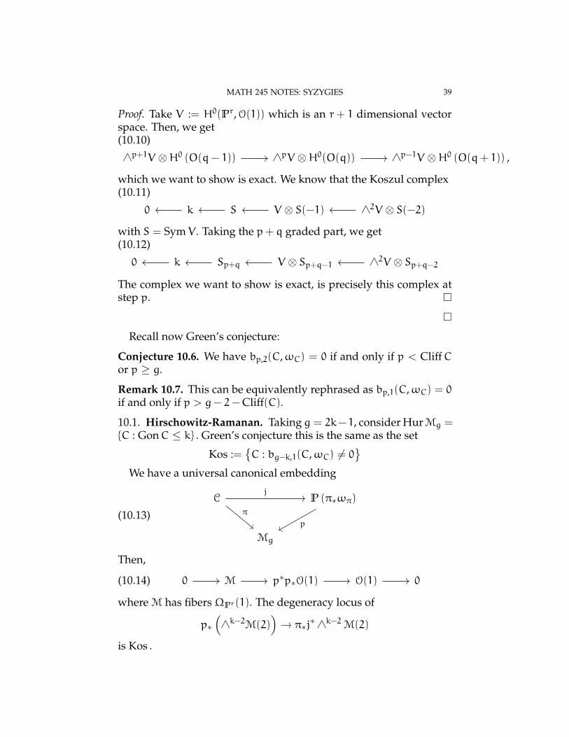
10.1. Hirschowitz-Ramanan. Taking g = 2k−1, consider HurMg =C : GonC ≤ k . Green’s conjecture this is the same as the set
Kos :=C : bg−k,1(C,ωC) 6= 0
We have a universal canonical embedding
(10.13)
C P (π∗ωπ)
Mg
j
π
p
Then,
(10.14) 0 M p∗p∗O(1) O(1) 0
where M has fibersΩPr(1). The degeneracy locus of
p∗(∧k−2M(2)
)→ π∗j∗ ∧k−2M(2)
is Kos .
40 AARON LANDESMAN
11. 5/8/17
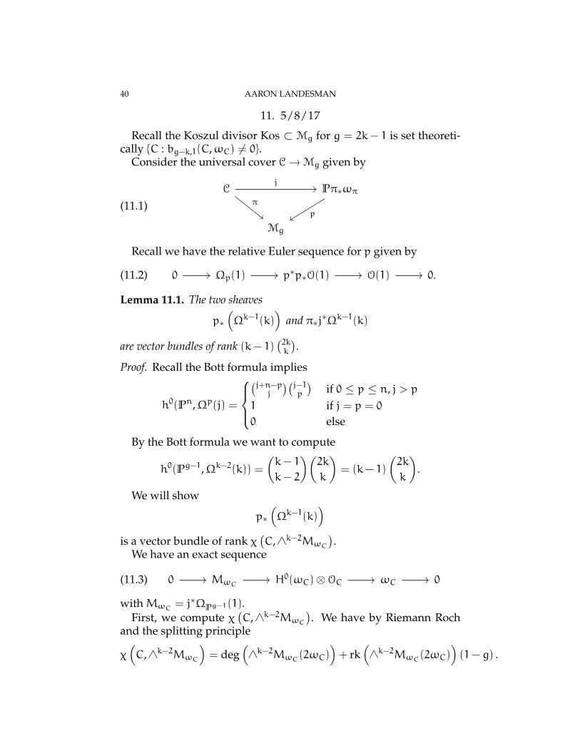
Recall the Koszul divisor Kos ⊂ Mg for g = 2k− 1 is set theoreti-cally C : bg−k,1(C,ωC) 6= 0.
Consider the universal cover C→Mg given by
(11.1)C Pπ∗ωπ
Mg
j
π
p
Recall we have the relative Euler sequence for p given by
(11.2) 0 Ωp(1) p∗p∗O(1) O(1) 0.
Lemma 11.1. The two sheaves
p∗(Ωk−1(k)
)and π∗j∗Ωk−1(k)
are vector bundles of rank (k− 1)(2kk
).
Proof. Recall the Bott formula implies
h0(Pn,Ωp(j) =
(j+n−pj
)(j−1p
)if 0 ≤ p ≤ n, j > p
1 if j = p = 0
0 else
By the Bott formula we want to compute
h0(Pg−1,Ωk−2(k)) =(k− 1
k− 2
)(2k
k
)= (k− 1)
(2k
k
).
We will show
p∗(Ωk−1(k)
)is a vector bundle of rank χ
(C,∧k−2MωC
).
We have an exact sequence
(11.3) 0 MωC H0(ωC)⊗OC ωC 0
withMωC = j∗ΩPg−1(1).First, we compute χ
(C,∧k−2MωC
). We have by Riemann Roch
and the splitting principle
χ(C,∧k−2MωC
)= deg
(∧k−2MωC(2ωC)
)+ rk
(∧k−2MωC(2ωC)
)(1− g) .
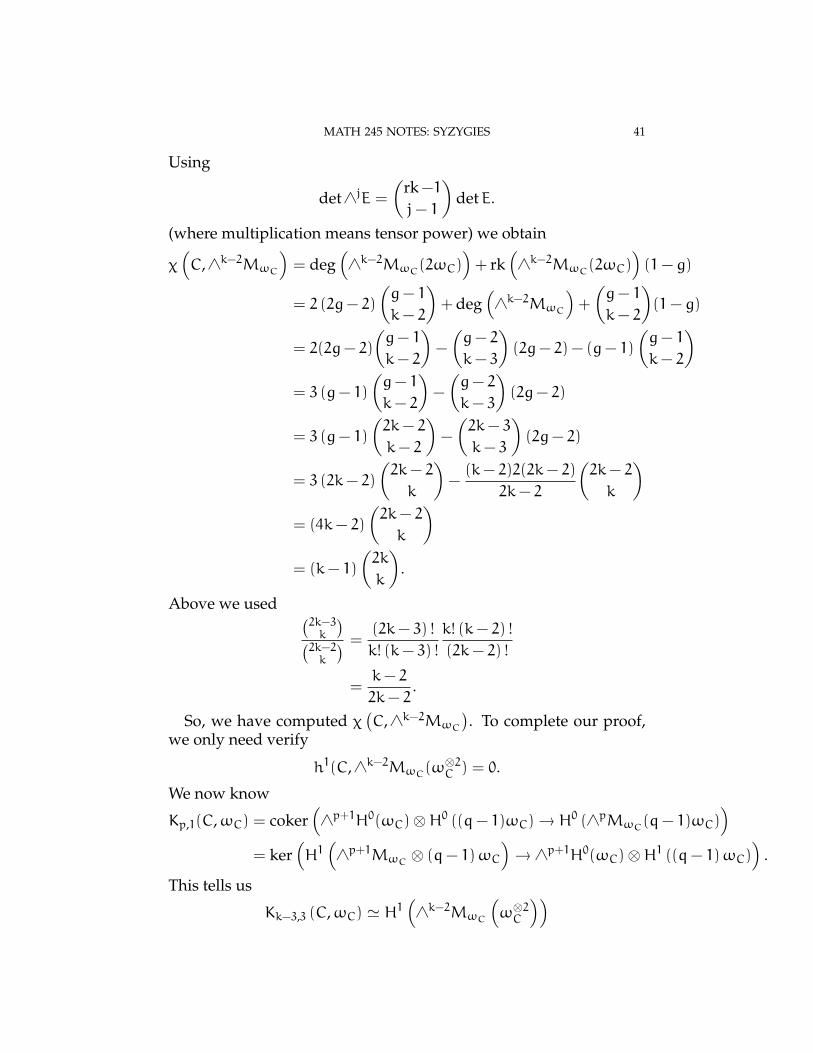
MATH 245 NOTES: SYZYGIES 41
Using
det∧jE =
(rk−1
j− 1
)detE.
(where multiplication means tensor power) we obtain
χ(C,∧k−2MωC
)= deg
(∧k−2MωC(2ωC)
)+ rk
(∧k−2MωC(2ωC)
)(1− g)
= 2 (2g− 2)
(g− 1
k− 2
)+ deg
(∧k−2MωC
)+
(g− 1
k− 2
)(1− g)
= 2(2g− 2)
(g− 1
k− 2
)−
(g− 2
k− 3
)(2g− 2) − (g− 1)
(g− 1
k− 2
)= 3 (g− 1)
(g− 1
k− 2
)−
(g− 2
k− 3
)(2g− 2)
= 3 (g− 1)
(2k− 2
k− 2
)−
(2k− 3
k− 3
)(2g− 2)
= 3 (2k− 2)
(2k− 2
k
)−
(k− 2)2(2k− 2)
2k− 2
(2k− 2
k
)= (4k− 2)
(2k− 2
k
)= (k− 1)
(2k
k
).
Above we used (2k−3k
)(2k−2k
) =(2k− 3) !
k! (k− 3) !
k! (k− 2) !
(2k− 2) !
=k− 2
2k− 2.
So, we have computed χ(C,∧k−2MωC
). To complete our proof,
we only need verify
h1(C,∧k−2MωC(ω⊗2C ) = 0.
We now know
Kp,1(C,ωC) = coker(∧p+1H0(ωC)⊗H0 ((q− 1)ωC)→ H0 (∧pMωC(q− 1)ωC)
)= ker
(H1(∧p+1MωC ⊗ (q− 1)ωC
)→ ∧p+1H0(ωC)⊗H1 ((q− 1)ωC))
.
This tells us
Kk−3,3 (C,ωC) ' H1(∧k−2MωC
(ω⊗2C
))
42 AARON LANDESMAN
as H1(ω⊗2C
)= 0. Serre duality tells us that
bk−3,3(C,ωC) = bk,0(C,ωC)
It suffices to show the following:
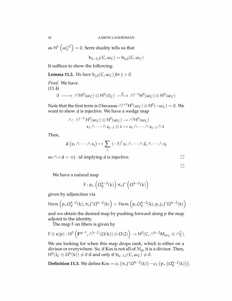
Lemma 11.2. We have bj,0(C,ωC) for j > 0.
Proof. We have(11.4)
0 ∧jH0(ωC)⊗H0(OC) ∧j−1H0(ωC)⊗H0(ωC)d
Note that the first term is 0 because ∧j+1H0(ωC)⊗H0(−ωC) = 0. Wewant to show d is injective. We have a wedge map
∧ : ∧j−1 H0(ωC)⊗H0(ωC)→ ∧jH0(ωC)
s1 ∧ · · ·∧ sj−1 ⊗ t 7→ s1 ∧ · · ·∧ sj−1 ∧ t
Then,
d(s1 ∧ · · ·∧ sj
)7→∑
j
(−1)i s1 ∧ · · ·∧ si ∧ · · ·∧ sj
so ∧ d = ±j · id implying d is injective.
We have a natural map
F : p∗(Ωk−2p (k)
)π∗j∗(Ωk−2(k)
)given by adjunction via
Hom(p∗Ω
k−2p (k),π∗j∗Ωk−2(k)
)= Hom
(p∗Ω
k−2p (k),p∗j∗j∗Ωk−2(k)
)and we obtain the desired map by pushing forward along p the mapadjoint to the identity.
The map F on fibers is given by
F⊗ κ(p) : H0(
Pg−1,∧k−2 (Ω(k))⊗O(2))→ H0(C,∧k−2MωC ⊗∧2C).
We are looking for when this map drops rank, which is either on adivisor or everywhere. So, if Kos is not all of Mg, it is a divisor. Then,H0(IC ⊗Ωk(k)) 6= 0 if and only if bk−1,1(C,ωC) 6= 0.
Definition 11.3. We define Kos = c1(π∗j∗Ωk−2(k)
)−c1
(p∗(Ωk−2p (k)
)).
MATH 245 NOTES: SYZYGIES 43
We now introduce some notation. Define
M := Ωp(1)
and define
Ga,b := p∗ ∧aM(b).
We have an Euler sequence
(11.5) 0 M p∗p∗O(1) O(1) 0.
This yields an exact sequence(11.6)
0 ∧wM ∧wp∗p∗O(1) ∧w−1M⊗O(1) 0
we obtain
R1p∗ ∧wM(q) = 0
for w ≥ 0,q > 0 as bw−1,q+1(Pg−1,O(1)
)= 0. Pushing forward the
above sequence via p yields(11.7)
0 p∗ (∧wM(q)) ∧wp∗O(1)⊗ p∗O(q) p∗(∧w−1M (q− 1)
)0
using the projection formula. We can rewrite this as(11.8)
0 Ga,b ∧aG0,1 ⊗G0,b Ga−1,b−1 0
Using this we can determine Chern classes by induction on a.
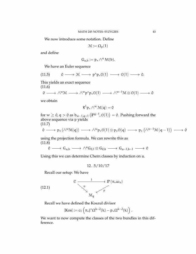
12. 5/10/17
Recall our setup: We have
(12.1)
C P (π∗ωπ)
Mg
j
π
p
Recall we have defined the Koszul divisor
[Kos] := c1(π∗j∗Ωk−2(k) − p∗Ω
k−2(k))
.
We want to now compute the classes of the two bundles in this dif-ference.
44 AARON LANDESMAN
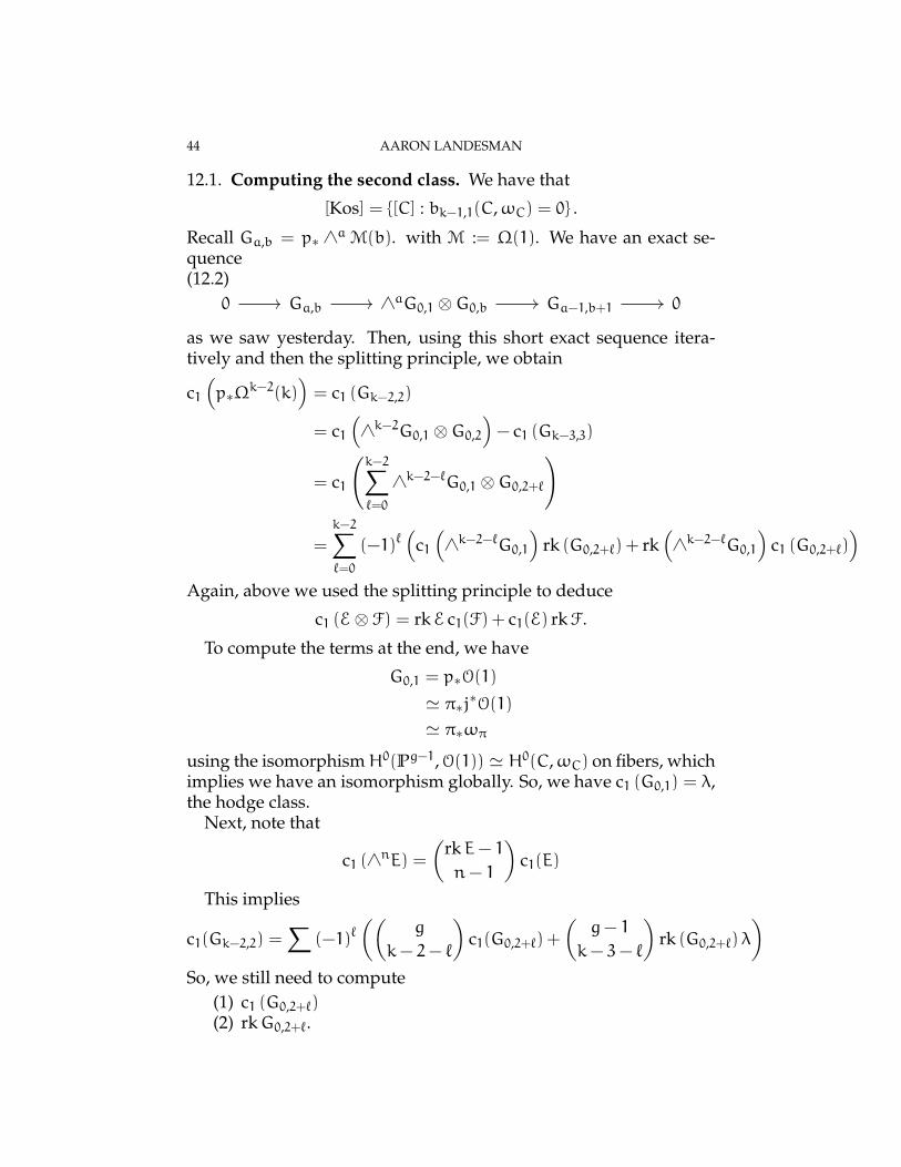
12.1. Computing the second class. We have that
[Kos] = [C] : bk−1,1(C,ωC) = 0 .
Recall Ga,b = p∗ ∧a M(b). with M := Ω(1). We have an exact se-quence(12.2)
0 Ga,b ∧aG0,1 ⊗G0,b Ga−1,b+1 0
as we saw yesterday. Then, using this short exact sequence itera-tively and then the splitting principle, we obtain
c1(p∗Ω
k−2(k))= c1 (Gk−2,2)
= c1(∧k−2G0,1 ⊗G0,2
)− c1 (Gk−3,3)
= c1
(k−2∑`=0
∧k−2−`G0,1 ⊗G0,2+`
)
=
k−2∑`=0
(−1)`(
c1(∧k−2−`G0,1
)rk (G0,2+`) + rk
(∧k−2−`G0,1
)c1 (G0,2+`)
)Again, above we used the splitting principle to deduce
c1 (E⊗ F) = rkE c1(F) + c1(E) rkF.
To compute the terms at the end, we have
G0,1 = p∗O(1)
' π∗j∗O(1)' π∗ωπ
using the isomorphismH0(Pg−1,O(1)) ' H0(C,ωC) on fibers, whichimplies we have an isomorphism globally. So, we have c1 (G0,1) = λ,the hodge class.
Next, note that
c1 (∧nE) =(
rkE− 1n− 1
)c1(E)
This implies
c1(Gk−2,2) =∑
(−1)`((
g
k− 2− `
)c1(G0,2+`) +
(g− 1
k− 3− `
)rk (G0,2+`) λ
)So, we still need to compute
(1) c1 (G0,2+`)(2) rkG0,2+`.
MATH 245 NOTES: SYZYGIES 45
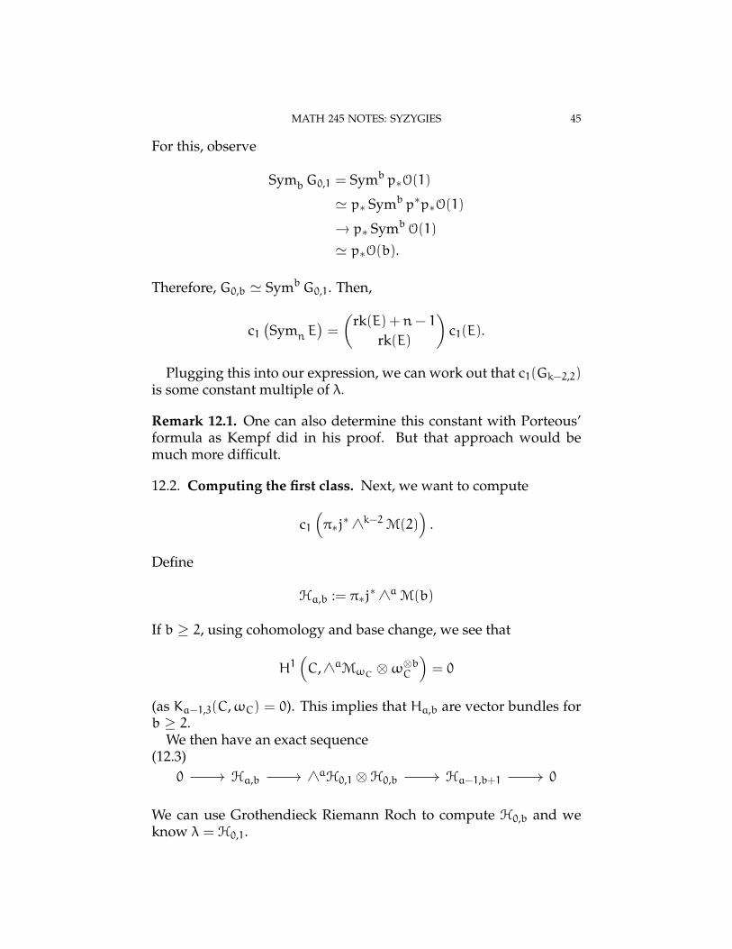
For this, observe
SymbG0,1 = Symb p∗O(1)
' p∗ Symb p∗p∗O(1)→ p∗ SymbO(1)
' p∗O(b).
Therefore, G0,b ' SymbG0,1. Then,
c1(Symn E
)=
(rk(E) +n− 1
rk(E)
)c1(E).
Plugging this into our expression, we can work out that c1(Gk−2,2)is some constant multiple of λ.
Remark 12.1. One can also determine this constant with Porteous’formula as Kempf did in his proof. But that approach would bemuch more difficult.
12.2. Computing the first class. Next, we want to compute
c1(π∗j∗ ∧k−2M(2)
).
Define
Ha,b := π∗j∗ ∧aM(b)
If b ≥ 2, using cohomology and base change, we see that
H1(C,∧aMωC ⊗ω⊗bC
)= 0
(as Ka−1,3(C,ωC) = 0). This implies that Ha,b are vector bundles forb ≥ 2.
We then have an exact sequence(12.3)
0 Ha,b ∧aH0,1 ⊗H0,b Ha−1,b+1 0
We can use Grothendieck Riemann Roch to compute H0,b and weknow λ = H0,1.
46 AARON LANDESMAN
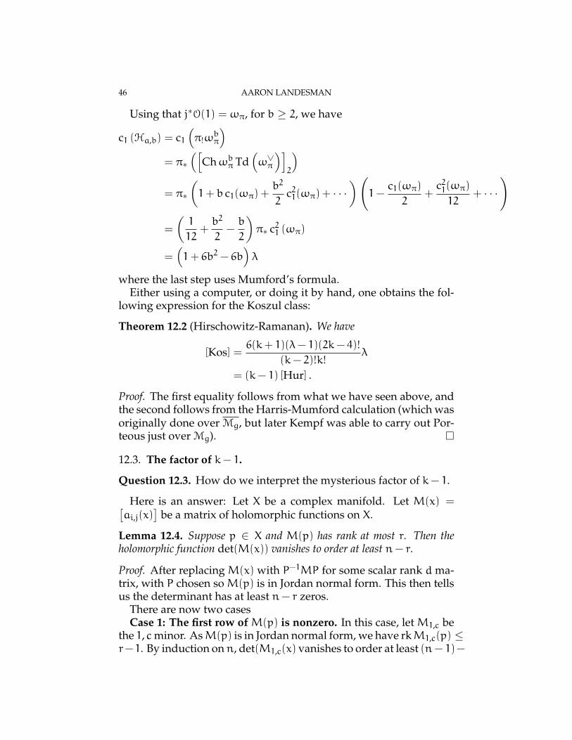
Using that j∗O(1) = ωπ, for b ≥ 2, we have
c1 (Ha,b) = c1(π!ω
bπ
)= π∗
([Chωbπ Td
(ω∨π
)]2
)= π∗
(1+ b c1(ωπ) +
b2
2c21(ωπ) + · · ·
)(1−
c1(ωπ)2
+c21(ωπ)12
+ · · ·)
=
(1
12+b2
2−b
2
)π∗ c21 (ωπ)
=(1+ 6b2 − 6b
)λ
where the last step uses Mumford’s formula.Either using a computer, or doing it by hand, one obtains the fol-
lowing expression for the Koszul class:
Theorem 12.2 (Hirschowitz-Ramanan). We have
[Kos] =6(k+ 1)(λ− 1)(2k− 4)!
(k− 2)!k!λ
= (k− 1) [Hur] .
Proof. The first equality follows from what we have seen above, andthe second follows from the Harris-Mumford calculation (which wasoriginally done over Mg, but later Kempf was able to carry out Por-teous just over Mg).
12.3. The factor of k− 1.
Question 12.3. How do we interpret the mysterious factor of k− 1.
Here is an answer: Let X be a complex manifold. Let M(x) =[ai,j(x)
]be a matrix of holomorphic functions on X.
Lemma 12.4. Suppose p ∈ X and M(p) has rank at most r. Then theholomorphic function det(M(x)) vanishes to order at least n− r.
Proof. After replacing M(x) with P−1MP for some scalar rank d ma-trix, with P chosen soM(p) is in Jordan normal form. This then tellsus the determinant has at least n− r zeros.
There are now two casesCase 1: The first row of M(p) is nonzero. In this case, let M1,c be
the 1, cminor. AsM(p) is in Jordan normal form, we have rkM1,c(p) ≤r−1. By induction onn, det(M1,c(x) vanishes to order at least (n− 1)−
MATH 245 NOTES: SYZYGIES 47
(r− 1) = n − r. This implies det (M(x)) vanishes to order at leastn− r.
Case 2: The first row of M(p) is 0. In this case, the result isstraightforward. Here we have det (M1,c(p)) vanishes to order atleast n− r− 1, the whole determinant vanishes to order at least n−r.
Proposition 12.5 (Hirschowitz-Ramanan). Let [C] ∈ Mg be a smoothpoint of the Hurwitz divisor. Then, bk−1,1(C,ωC) ≤ k− 1.Remark 12.6. In fact, the reverse inequality follows easily from theeagon northcott complex. That is, we have
bk−1,1(C,ωC) ≥ k− 1.
13. 5/12/17
We’ll start with explaining why scrolls come up. We’ll describe therelation between syzygies of curves and syzygies of scrolls.
Last time, we saw the Hirschowitz Ramanan computation impliesthat for a curve C ∈ Hur which is a smooth point of Hur, thenbk−1,1(C,ωC) ≤ k − 1 [Kos]
[Hur] . In fact, the reverse inequality holds aswell.
We will show that for any [C] ∈ Hur we also have the reverseinequality.
Lemma 13.1. For every curve C ∈ Hur, we have bk−1,1(C,ωC) ≥ k− 1.Proof. This follows by using the scroll in which the curve lies. Byupper semicontinuity, it suffices to show that for a general curveC ∈ Hur we have bk−1,1(C,ωC) ≥ k − 1. Let f : C → P1 be abase point free pencil of degree k. Let X be the associated scroll withC ⊂ X ⊂ Pg−1 so that the rulings of the scroll cut out the basepointfree pencil on the curve. Thanks to the eagon Northcott complex,we know ΓX(H) has a minimal free resolution of length k− 1, withH = OX(1), and bk−1,1(X,H) = k− 1. The claim then follows imme-diately from the following proposition.
Proposition 13.2. The restriction OX → OC induces an inclusion bp,1(X,H)→bp,1(C,ωC).
Remark 13.3. This says, geometrically, that some of the syzygies ofthe curve come from syzygies of the scroll.
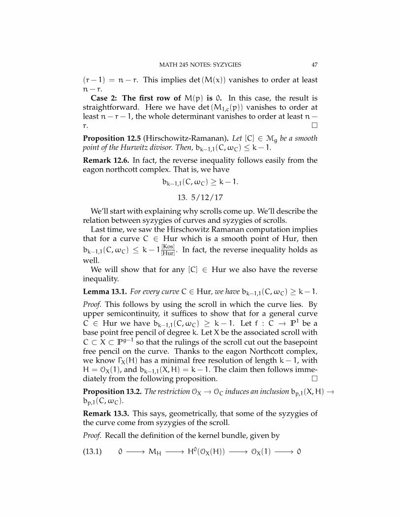
Proof. Recall the definition of the kernel bundle, given by
(13.1) 0 MH H0(OX(H)) OX(1) 0
48 AARON LANDESMAN
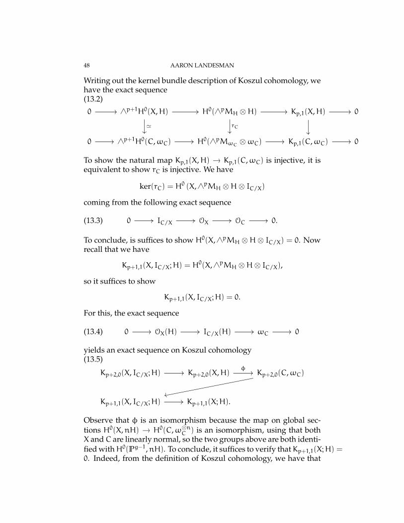
Writing out the kernel bundle description of Koszul cohomology, wehave the exact sequence(13.2)
0 ∧p+1H0(X,H) H0(∧pMH ⊗H) Kp,1(X,H) 0
0 ∧p+1H0(C,ωC) H0(∧pMωC ⊗ωC) Kp,1(C,ωC) 0
' rC
To show the natural map Kp,1(X,H) → Kp,1(C,ωC) is injective, it isequivalent to show rC is injective. We have
ker(rC) = H0 (X,∧pMH ⊗H⊗ IC/X)
coming from the following exact sequence
(13.3) 0 IC/X OX OC 0.
To conclude, is suffices to show H0(X,∧pMH ⊗H⊗ IC/X) = 0. Nowrecall that we have
Kp+1,1(X, IC/X;H) = H0(X,∧pMH ⊗H⊗ IC/X),
so it suffices to show
Kp+1,1(X, IC/X;H) = 0.
For this, the exact sequence
(13.4) 0 OX(H) IC/X(H) ωC 0
yields an exact sequence on Koszul cohomology(13.5)
Kp+2,0(X, IC/X;H) Kp+2,0(X,H) Kp+2,0(C,ωC)
Kp+1,1(X, IC/X;H) Kp+1,1(X;H).
φ
Observe that φ is an isomorphism because the map on global sec-tions H0(X,nH) → H0(C,ω⊗nC ) is an isomorphism, using that bothX andC are linearly normal, so the two groups above are both identi-fied withH0(Pg−1,nH). To conclude, it suffices to verify thatKp+1,1(X;H) =0. Indeed, from the definition of Koszul cohomology, we have that
MATH 245 NOTES: SYZYGIES 49
this is the middle cohomology of the complex
(13.6)
∧p+2H0(X,H)⊗H0(X, IC/X)
∧p+1H0(X,H)⊗H0(X,H⊗ IC/X)
∧pH0(X,H)⊗H0(X, 2H⊗ IC/X).
So, it suffices to show
∧p+1H0(X,H)⊗H0(X,H⊗ IC/X) = 0.
In turn, it suffices to verify
H0(X,H⊗ IC/X) = 0,
which holds by the crucial assumption that C is linearly normal.
13.1. K3 Surfaces.
Definition 13.4. A K3 surface is a smooth projective surface X withKX ' OX and H1(OX) = 0.
Lazarsfeld and Voisin studied Brill Noether theory and syzygiesusing K3 surfaces. Let C ⊂ X be a smooth curve. We want to relateL, a line bundle on a curve C to the study of vector bundles on a K3surface. The basic construction is due to Mukai:
Construction 13.5. Let L be a line bundle on a curve C ⊂ X andsuppose L is base point free. We have an evaluation map
ev : H0(C,L)⊗OC → L.
We studied MC = ker ev. We next construct a related line bundle onX.
Let i : C → X be a closed immersion. We define the Lazarsfeld-Mukai bundle FL as the kernel
(13.7) 0 FL H0(C,L)⊗OX i∗L 0
Proposition 13.6. The Lazarsfeld-Mukai bundle FL constructed in Con-struction 13.5 is locally free.
Proof. The claim is local, so we may assume L is trivial. Then, wehave an exact sequence
(13.8) 0 FL H0(C,L)⊗OX i∗OC 0
50 AARON LANDESMAN
Remark 13.7. Recall that the homological dimension of an R-moduleM is the minimal length of a projective resolution. By Auslander-Buchsbaum formula relates the homological dimension to depth. Thatis,
dh(M) + depth(M) = dimR.
For E a coherent sheaf, we have
dh(E) = max Ex : x ∈ X .
As follows from the Auslander-Buchsbaum formula and inequalitieson depth, if we have a short exact sequence of coherent sheaves
(13.9) 0 E F G 0
for F free, we have
dh(E) = max 0, dh(G) − 1 .
Using the above, it is equivalent to show that dh(OC) = 1. Butindeed this follows because homological dimension is the minimallength of a projective resolution, and we have a length 1 resolution
(13.10) 0 OX(−C) OX OC 0
so dh(OC) = 1.
14. 5/15/17
Today, we’ll discuss using K3 surfaces to understand curves.
14.1. Interlude on the Picard group of a K3 surface.
Definition 14.1. Let X be a smooth projective variety. A cycle ofcodimension r is an element Z of the free abelian group over Z,Zr(X), generated by closed irreducible subschemes of codimensionr.
We have the following three notions of equivalence for cycles:
Definition 14.2. Two cycles Z1,Z2 ∈ Zr(X) are rationally equivalentdenoted Z1 ∼rat Z2 if there exists a closed subscheme V ⊂ X× P1,flat over P1 so that
V ∩ X× 0 = Z1
V ∩ X× ∞ = Z2
MATH 245 NOTES: SYZYGIES 51
We define the Chow group
Ar(X) := Zr(X)/ ∼rat
Further, Pic(X) = A1(X).
Definition 14.3. Two cycles Z1,Z2 ∈ Zr(X) are algebraically equiv-alent denoted Z1 ∼alg Z2 if there exists smooth curve C and a closedsubscheme V ⊂ X×C, flat over Cwith two points p,q ∈ C so that
V ∩ X× p = Z1
V ∩ X× q = Z2
The Neron-Severi group is
NS(X) := Z1(X)/ ∼alg
Remark 14.4. It turns out the Neron-Severi group is the set of con-nected components of the Picard group.
Theorem 14.5 (Neron-Severi). NS(X) is a finitely generated abelian group.
Definition 14.6. Let X be a surface. Two invertible sheaves L1,L2 arenumerically equivalent, denoted L1 ∼num L2 if for all M ∈ Pic(X)we have
(L1 ·M) = (L2 ·M)
Remark 14.7. Note that L1 ∼alg L2 implies L1 ∼num L2. We furtherdefine num(X) = Pic(X)/ ∼num.
Remark 14.8. num(X) is a quotient of NS(X), hence num(X) is finitelygenerated. Further, num(X) turns out to be free.
This is because if Ln = OX, we obtain L ∼num OX because 0 =Ln ·M = nL ·M, which implies L ·M = 0.
Proposition 14.9. Let X be a K3 surface over the complex numbers. Thenthe natural maps
Pic(X)→ NS(X)→ num(X)
are all isomorphisms. In particular, Pic(X) ' Zr(X) for some integer r(x).
Proof. Assume L is numerically trivial. Then, for any ample line bun-dle H with L · H = 0. Assume L 6= OX. This implies that neitherL nor L∨ are effective, since the intersection of an ample with anycurve is positive (as we can take a high enough power of L whichis very ample and moves in a pencil, and then has positive intersec-tion).
52 AARON LANDESMAN
We then have by Serre duality that
h0(L) = 0 = h2(L) = h0(L∨).
Then,
−h1(L) = χ(L) =1
2(L · L+ωX) + χ(OX) =
1
2L2 + 2
Therefore,1
2(L)2 + 2 ≤ 0
and so
L2 < 0
which contradicts numerical triviality of L.
Definition 14.10. Let X be a K3 surface and fix an ample line bundleH. For a coherent sheaf F ∈ coh(X), define the rank of F to be its rankas a sheaf over the generic point (i.e., the rank of the correspondingmodule over K(X)).
Define the slope of F to be
µ(F) :=degH F
rk(F).
Definition 14.11. Let F be. Then F is said to be H-stable if for allsubsheaves 0 ( E ( Fwith 0 < rkE < rk F, we have
µ(E) < µ(F).
Example 14.12. The sheaf H⊕OX is not stable. To see why, note thatc1(H+OX) = H. Therefore, µ(H⊕OX) = H
2/2 > 0. But,
µ(H) = H2 > H2/2 = µ(H⊕OX)
Remark 14.13. Slope stability is a useful condition for controllingthe automorphisms groups. This yields an analogy between stablevector bundles and stable curves. We now explain this further.
Proposition 14.14. Let F be H-stable. Then, any nonzero endomorphismφ : F → F is an isomorphism.
Proof. Suppose ψwere not an isomorphism. Then, we claim kerψ 6=0. To see this, if ψwere injective, we would have
(14.1) 0 F F G 0
which implies that ci(G) = 0 for all i and the rank is 0 (by additivityof rank in short exact sequences). This implies that in fact G = 0.
MATH 245 NOTES: SYZYGIES 53
Therefore, ψ is not injective. Hence, we have some kernel
(14.2) 0 G F F
Thus, G ⊂ F is some nonzero subbundle. Note that G is also torsionfree because it is a subsheaf of F, which is torsion free by assumption.Hence, rk(F) > rk(G) ≥ 1. Which implies rk im φ < rkF. We nowapply stability to im φ ( F.
Using stability, we have
µ (im φ) < µF.
We have a short exact sequence
(14.3) 0 kerφ F im φ 0
Since degree and rank are additive, we have
degF = deg kerφ+ deg im φ rkF = rk kerφ+ rk im φ
We then obtain
µ(F) − µ(kerφ) =rk im φ
rk kerφ(µ(im φ) − µF) .
We know the right hand side is negative. But, by stability of F, theleft hand side is positive, a contradiction.
14.2. Stability of Lazarsfeld-Mukai bundles. Recall the setup fromlast time. Let i : C ⊂ X be a curve and let A ∈ PicC be a basepointfree line bundle. Then, we construct FA as the kernel
(14.4) 0 FA H0(A)⊗OX i∗A 0.
Proposition 14.15. Assume the Picard rank ρ(X) = 1 and PicX = Z [C]and H := OX(C). Then, FA is stable.
Proof. For any vector bundle which is a subsheaf of a free sheaf V ⊂O⊕aX and any 1 ≤ s ≤ rk(V), consider ∧sV∨ as a vector bundle. Letb =
(as
). We then have ∧sV ⊂ O⊕bX . Therefore,
EndOX(∧sV) ' ∧sV ⊗∧sV∨ ⊂
(∧sV∨
)⊕b.
It follows
0 6= id ∈ H0 (End (∧sV))
Therefore, H0(∧sV∨
)≥ 1.
54 AARON LANDESMAN
Now, let E ⊂ FA be a subsheaf with rkE < rk FA. By the above,taking s = rkE, and noting that E ⊂ FA ⊂ OX ⊗H0(A), we see
h0(detE∨) ≥ 1h0(∧e−1E∨) ≥ 1.
Then, since detE has a section, we conclude detE = kH∨ for k ≥ 0.Lemma 14.16. We have detE 6= 0. That is, k 6= 0 above.
Proof. Note that
E ' ∧e−1E∨ ⊗ detE.
Since k = 0, we have E ' ∧e−1E∨, and so E would then have asection. Taking cohomology for the exact sequence, we get
(14.5) FA H0(A)⊗OX i∗A,
we see
(14.6) 0 H0(FA) H0(A) H0(A)'
which implies H0(FA) = 0 and so H0(E) = 0.
So, we know k > 0. Then,
det FA = − c1(im A) = − c1(OC).
This implies i∗A ' OC outside of codimension 2. Hence, from theshort exact sequence
(14.7) 0 OX(−C) OX OC 0
we obtain c1(OC) = c1(OX(C)) It follows that det FA = − [C] = −H.Since these degrees are negative, and the rank of E is less than thatof A, we obtain rk(E) < rk(F), using that k > 0.
15. 5/17/17
15.1. Hirzebruch-Riemann-Roch for K3 surfaces. Let us start byrecalling Hirzebruch-Riemann-Roch: For E a vector bundle and Xsmooth and projective then
χ(E) =
∫X
c(E) · Td(X)
where integration means taking the top degree piece. Here, Td(X) =Td(TX).
Lemma 15.1. For X a K3 surface, we have deg c2(TX) = 24.
MATH 245 NOTES: SYZYGIES 55
Proof. If X is a K3 surface, then c1(TX) = 0. Therefore,
2 = χ(OX)
= deg[1+
c12+1
12(c2+ c2)
]2
This implies 12 · 2 = deg c2 (TX). Hence, deg c2(TX) = 24.
Recall that
Ch(E) = rkE+ c1(E) +1
2
(c21(E) − 2 c2(E)
).
Corollary 15.2. For X a K3 surface and E any vector bundle, we have
χ(E) = deg (Ch2(E) + 2 rk(E)) .
Proof. This follows by plugging in the result of the previous lemmato Hirzebruch-Riemann-Roch.
15.2. Recollection of Brill-Noether theory. Let C be a curve andA ∈ Pic(C). Recall the Brill-Noether number
ρ(A) := g− h0(A)h1(A).
This is the “expected dimension” of the locus of line bundles of de-
gree degA and h0(A) sections. We letWh0(A)−1degA denote this locus.
We’ll give a simple argument due to Lazarsfeld for that a generalcurve the dimension ofWr
d is the expected dimension.Assume C ⊂ X is a K3 surface. Let A be basepoint free. Recall
(15.1) 0 FA H0(C,A)⊗OX i∗A 0
Proposition 15.3. ForA a basepoint free invertible sheaf on a curveCwithC ⊂ X for X a K3 surface, we have
χ(FA ⊗ F∨A
)= 2− 2ρ(A).
Proof. Ch gives a ring homomorphism from the K group to the chowring. That is,
Ch(FA ⊗ F∨) = Ch(FA) ·Ch(F∨A).
56 AARON LANDESMAN
Exercise 15.4. Let
ct(E) = 1+ c1(E)t+ c2(E)t2 + · · ·= (1+ a1(E)t) · · · (1+ as(E)t)
and comparing ct(E) to
ct(E∨) = 1+ c1(E∨)t+ c2(E∨)t2 + · · ·= (1− a1(E)t) · · · (1− as(E)t) .
Show using the above and the splitting principle that
ci(E∨) = (−1)i ci(E).
By the above, we have
Ch(FA) = rk(FA) + c1(FA) +1
2
(c21(FA) − 2 c2(FA)
)Ch(F∨A) = rk(FA) − c1(FA) +
1
2
(c21(FA) − 2 c2(FA)
).
Letting e = h0(C,A) and L = [C], we have
rk FA = e
c1 FA = −L
We using the exact sequence
(15.2) 0 FA H0(C,A)⊗OX i∗A 0
and the facts that χi∗A = χ(C,A) (we saw this last time, but essen-tially it follows because the two agree outside a codimension 2 set)and χ(OX) = 2, we have
2e = χ(FA) + χ(C,A)= χ(FA) + (d+ 1− g).
Hence, using Hirzebruch Riemann Roch as above, we get χ(FA) =Ch2(FA) + 2 rk(FA), and so
2e+ Ch2(FA) + d+ 1− g = 2e
It follows1
2L2 − c2(FA) = g− 1− d.(15.3)
We have an exact sequence
(15.4) 0 OX L OC(C) 0
MATH 245 NOTES: SYZYGIES 57
Note that OC(C) = ωC by adjunction because KX = OX. Therefore,
χ(L) − 2 = g− 1.
Using this and Riemann-Roch (on surfaces) which says χ(L) = 12L ·
(L+KX) + 2, we obtain1
2L2 = g− 1.
We then obtain, by plugging in the previous line to Equation 15.3
c2(FA) = d,
Collating this, and using Hirzebruch-Riemann-Roch, we have
χ(FA ⊗ F∨A
)=[2 rk
(FA ⊗ F∨A
)+ Ch2
(FA ⊗ F∨A
)]= 2e2 + Ch2(FA)
Therefore,
χ(FA ⊗ F∨A
)= 2e2 + e (2g− 2− 2d) − (2g− 2) .
Therefore, since
ρ(A) = g− e (e+ g− d− 1) ,
with e+ g− d− 1 = h1(A). It follows that
χ(FA ⊗ F∨A
)= 2− 2ρ(A).
15.3. Brill Noether on K3 surfaces.
Definition 15.5. Let k be a field with ch k = 0, X a variety over kand E a vector bundle on X. We say a vector bundle E is simple ifHom(E,E) = k.
Lemma 15.6. Assume PicX = Z [C] and FA as above the Lazarsfeld-Mukai bundle associated to A on C ⊂ X. Then, FA is simple.
Proof. We know FA is stable, so any nonzero morphism φ : FA → FAis an isomorphism. We claim φ is constant. Assume otherwise. Pickany x ∈ X. Then, φ⊗ k(x) is a matrix. Pick any eigenvalue λ. Thenφ− λidis not an isomorphism and is nonzero, a contradiction.
We deduce the following result in Brill-Noether theory.
Proposition 15.7. Let C ⊂ X be a smooth curve and Pic(X) ' Z [C].Then, for any A ∈ Pic(C) we have ρ(A) ≥ 0.
58 AARON LANDESMAN
Proof. Assume A is basepoint free. Then,
χ(FA ⊗ F∨A
)=(FA ⊗ F∨A
)− h1
(FA ⊗ F∨A
)+ h2(FA ⊗ F∨A)
= 2− h1(FA ⊗ F∨A.
).
Therefore,
2− 2ρ(A) = 2g− h1(FA ⊗ F∨A),which implies ρ(A) ≥ 0.
If A is not basepoint free, let Z be the base locus. Then, A(−Z) isbasepoint free. Then,
deg(A(−Z)) < deg(A)
h0(A(−Z)) = h0(A)
This implies
0 < ρ (A(−Z)) < ρ(A)
15.4. Deformation theory of Hilbert schemes. One reference for thissection is Sernesi’s book on deformation theory. We now state themain results on properties of the Hilbert scheme.
Let X ⊂ Pr be a projective variety and fix a polynomial p(t) ∈Q [t]. The Hilbert functor HY
p(t) assigns to any scheme locally noe-therian S-scheme all flat morphisms
(15.5)X X× S
S
so that each fiber has Hilbert polynomial p(t).
Theorem 15.8. The functor HYp(t) is representable by a schemeH. Further,
there is a universal family Z ⊂ Y × H, flat over H which is universal,meaning that for any S and X ⊂ Y × S in HY
p(t)(S) so that there is a fibersquare
(15.6)X Z
S H
We have the following result on deformation theory:
MATH 245 NOTES: SYZYGIES 59
Theorem 15.9. Assume Y is smooth and let [X ⊂ Y] ∈ H(Spec k) whereX is smooth. Then,
(1) TX(H) ' H0(X,NX/Y)
(2) If H1(X,NX/Y) = 0 then H is smooth at [X].
16. 5/22/17
Today’s objective is to prove Lazarsfeld’s Brill Noether theorem.We’ve already seen that on a K3 surface of Picard rank 1, the corre-spondingWr
d is empty. Lazarsfeld’s theorem says that when ρ(g, r,d) >0, allWr
d’s are smooth of the expected dimension ρ.
Definition 16.1. Fix r,d > 0 and let X be a K3 surface with PicX 'ZL. Fix an isomorphism V ' Cr+1. Define Prd to be the schemeparameterizing tuples (C,A, λ) so that
(1) C ∈ |L| is smooth and irreducible(2) A ∈Wr
d(C) is base point free(3) λ is a surjection
V ⊗OX i∗A
so that
H0(λ) : V ' H0(C,A).
modulo the equivalence relation that
(C,A, λ) ∼ (C,A,aλ)
with a ∈ C − 0.
Lemma 16.2. The functor Prd is a open subscheme of the Hilbert schemeH(X×P(V)), contained in a single component of the Hilbert scheme (i.e.,there is a single Hilbert polynomial associated to the Hilbert scheme inwhich Prd lies.
Proof. The triple (C,A, λ) determines
λ|C : V ⊗OC → A
which yields a morphism C→ P(V). Since we started with a closedimmersion C → X we hence have a closed immersion C ⊂ X×PV .Conversely, given such a closed embedding, we obtain (C,A, λ), andthese two constructions are clearly mutually inverse. We are justusing that λ|C being a surjection is an open condition.
60 AARON LANDESMAN
There is a morphism
π : Prd → P|L|
(C,A, λ) 7→ C ∈ |L|
where |L| := PH0(L). We want to study the differential of π. A triple(C,A, λ) ∈ Prd corresponds to C ⊂ X×P(V). We obtain g : C→ PV .Here g = φA. We then have a short exact sequence
(16.1) 0 g∗TPV NC/X×P(V) NC/X 0α
Hence,
T(C,A,λ)Prd = H0(C,NC/X×PV).
We have
TC,λ|L| = H0(C,NC/X)
= H0(C,OC(C))
= H0(C,ωC).
We can identify dπ at (C,A, λ) with H0(α).
Theorem 16.3 (Lazarsfeld). Assume PicX ' ZL. Then, dπ(C,A,λ) issurjective if and only if Petri’s multiplication map
µ : H0(C,A)⊗H0(C,ωC −A)→ H0(C,ωC)
is injective.
Proof. To start, recall the short exact sequence
(16.2) 0 g∗TPV NC/X×PV NC/X 0α
We have the following claim:
Lemma 16.4. The map H1(α) is an isomorphism.
Proof. We know H2(C,g∗TPV) = 0 so H1(α) is surjective. Second, weknow h1(NC/X) = h
1(ωC) = 1. So, it suffices to show h1(NC/X×PV) =1. For this, let us describe the embedding C ⊂ X×PV with projec-tions pr1 : X× PV → X, pr2 : X× PV → PV . We can canonicallyidentify
V ' H0 (PV ,O(1)) .
We have an exact sequence
(16.3) 0 FA V ⊗OλX i∗A 0φ
MATH 245 NOTES: SYZYGIES 61
Then φ induces a morphism
pr∗1(FA)⊗ pr∗2 O(−1)→ OX×PV .
This map sends S⊗ T 7→ T (φ(S)). We obtain a global section z of
pr∗1(F∨A
)⊗ pr∗2 O(1).
We can check from the exact sequence (16.3) Z(z) = C ⊂ X×PV . Itfollows that
NC/X×PV ' F∨A|C ⊗A|C
We need h1(X, F∨ ⊗ i∗A
)= 1. This is the same as the restriction to
C because i∗A is supported on C.Tensoring our definition of FA by F∨A we get
(16.4) 0 FA ⊗ F∨A V ⊗ F∨A A⊗ F∨A 0.
Since FA is simple, using Serre duality, we have
h0(FA ⊗ F∨A) = h2(FA ⊗ F∨A) = 1.
Then,
h2(V ⊗ F∨A
)= dimV · h2(F∨A) = dimV · h0(FA) = 0,
as follows from the sequence
(16.5) 0 FA V ⊗OX i∗A 0η
and the fact that H0(η) is an isomorphism. To show the map
H1(A⊗ F∨)→ H2(FA ⊗ F∨A) ' C
is an isomorphism, which would complete the proof, it only remainsto check H1(V ⊗ F∨A).
Indeed, this follows becauseH1(OX) = 0 and so from the sequence
(16.6)
0 h0(FA) V H0(i∗A
h1(FA) 0
H0(λ)
This implies H1(FA) = 0 since H0(λ) is an isomorphism. Hence,H1(F∨A) = 0, as we wanted to show.
62 AARON LANDESMAN
So, we have seen H1(α) is an isomorphism. We want to show thepetri map is injective if and only if dπ is surjective.
We have an exact sequence(16.7)
0 H0(C,g∗TPV) H0(NC/X×PV) H0(NC/X)
H1(g∗TPV) 0
dπ
Then, dπ is surjective if and only if H1(g∗TPV) = 0.To complete the proof, it suffices to check H1(C,g∗TPV) = 0 if and
only if the Petri map is injective.Here, g = φA : C → PV , up to a choice of basis. Then, the result
follows from Petri’s theorem, which we’ll talk about next time.That is, Petri’s theorem says:
Theorem 16.5 (Petri).
H1(C,g∗TPV)∨ = ker
(µ : H0(ωC −A)⊗H0(A)→ H0(ωC)
).
This tells us dπ is surjective if and only if µ is injective.
17. 5/24/17
Today, we’ll discuss the Petri map.
Definition 17.1. Given a curve C and a line bundle L on C, the petrimap is
µ : H0(L)⊗H0(ωC − L)→ H0(∧C).
Late time, we studied the map p : Prd → |L|. sending (C,A, λ) 7→C. We saw that generic smoothness of the map p implies that thedifferential is surjective, which means µA is injective.
Today’s goal will be to relate this to Brill-Noether theory.
17.1. The construction ofWrd(C). Let L be a Poincare bundle onC×
Picd(C), meaning that L|C×[M] = M on C. These are determined upto pullback of a bundle from Picd(C). Let q : C× Picd(C)→ Picd(C)be the projection.
Fix a divisor E on C of degree 2g− d− 1. Here, g = g(C). Let
F := E× Picd(C) ⊂ C× Picd(C).
MATH 245 NOTES: SYZYGIES 63
We get an exact sequence
(17.1) 0 L(−F) L L|F 0
and twisting by Fwe get
(17.2) 0 L L(F) L|F(F) 0
For any L ∈ Picd(C) we have that degL(E) ≥ 2g− 1 so
h1(C,L(E)) = 0.
From Grauert’s formula,
R1q∗L (F) = 0.
Pushing forward the exact sequence above by q, we get the exactsequence(17.3)
0 q∗L q∗L(F) q∗ (L|F(F)) R1q∗L 0f
Let
A := q∗L(F)
B := q∗L|F(F).
Both A and B are vector bundles by Grauert’s theorem. Further,pushforward commute with base change, so we obtain
f⊗ k(p) : H0(C,L(E))→ H0(C,L|E(E)).
Choose [L] = P ∈ Picd(C). Pick H0(C,L) ≥ r+ 1. Then the rank off⊗ κ(p) is at most 2g− d− 1+m− (r+ 1). We define Wr
d(C) as thelocus of points p so that f : A→ B has rank at most 2g− d− 1+m−(r+ 1).
We saw long ago how to construct such loci in a functorial way viafitting ideals:
Set
OWrd(C):= OPicd(C)/Ij(f),
where Ij(f) is the fitting ideal. Recall the definition: We have a map
∧jf : ∧jA→ ∧jB ∈ Hom(∧jA,∧jB)
' ∧jA∨ ⊗∧jB
' Hom(∧jA⊗∧jB∨,OPicd(C)
).
64 AARON LANDESMAN
Under this correspondence, we define Ij(f) as the image of ∧jf inOPicd(C). The key property that we talked about in lecture 6 or so isthat Ij(f) is functorial. That is, it commutes with base change. Thatis, Ij (f⊗ Spec B) = Ij(f)⊗ Spec B. Loosely speaking “fitting idealsare independent of presentation.”
Let’s try to understand
T[L]Wrd(C) ⊂ T[L] Picd(C) ' H1(C,OC) ' H0(ωC)∨.
We wish to describe those L ′ ∈ Picd (C× Spec k [ε]) reducing to L
which come from elements of T[L]Wrd(C). That is we want to charac-
terize first order deformations of L so that the sections s1, . . . , sr+1 ofH0(C,L) also deform.
We can describe a line bundle L via transition functions. That is, Lis the same as the data Uα together with transition functions
gαβ ∈ O×(Uα ∩Uβ
).
Let
Uα := Uα × Spec k [ε] ,gαβ
be the transition data for L ′. As L ′ reduces to L, we have
gαβ = gαβ(1+ εhαβ).
Then,
hαβ ∈ O×(Uα ∩Uβ
).
Then, these gαβ satisfy the cocycle relation, which means
gαβgβγ = gαγ.
We obtain
gαβ(1+ εhαβ
)gβγ
(1+ εhβγ
)= gαγ (1+ εhαγ)
so
gαβgβγ(1+ ε
(hαβ + hβγ
)). = gαγ (1+ εhαγ) .
Comparing the ε coefficient, we obtain
gαγ(hαβ + hβγ
)= gαγ(hαγ).
It follows that
hαβ + hβγ = hαγ.
We want to understand when a section s ∈ H0(C,L) lifts to a sec-tion of L ′.
MATH 245 NOTES: SYZYGIES 65
In terms of transition data, a section is a collection
sα , sα ∈ Γ(OUα) such that sα = gαβsβ.
Then, an extension s of s to a global section of L ′ is
sα , sα ∈ Γ(OUα
)satisfying the two conditions that
(1)
sα = sα + εs′α
(2)
sα = gαβsβ
Expanding the second equation, we get
sα + εs′α = sα
= gαβ · sβ= gαβ
(1+ εhαβ
) (sβ + εs
′β
).
Expanding this and comparing coefficients of ε, we see
s ′α = gαβs′β + gαβhαβsβ
This can be simplified slightly to
hαβsα = s ′α − gαβs′β.
By the property that
hαβ + hβγ = hαγ,
we have that h is a 1-cocycle in C1 (Uα , OUα) . That is, it deter-mines an element z ∈ H1(C,OC). In other words, the tangent spaceto the Picard group is H1(C,OC) = T[L] Picd(C). Here, z correspondsto L ′. Further, z⊗ s = hαβsα ∈ H1(C,L). The condition for s toextend is saying z⊗ s = 0 because
hαβsα = s ′α − gαβs′β = δ
(s ′α)∈ C0 (Uα , Lα) .
Theorem 17.2. So, assume that L ∈Wrd(C) has r+ 1 sections. Then,
T[L]Wrd(C) =
z ∈ H1 (OC) : z⊗H0 (C,L) = 0
∈ H1(C,L).
Equivalently, using Serre duality,
T[L]Wrd(C) = (im µ)⊥
For µ the petri map.
66 AARON LANDESMAN
18. 5/26/17
18.1. Wrapping up the Petri map. Assume L ∈Wrd(C) with h0(C) =
r+ 1. We saw
v ∈ H1(C,OC) ' Picd(C)
lies in
T[L]Wrd(C)
if and only if
v⊗H0(C,L)→ H1(C,L)s 7→ s⊗ v
is the zero map.
Lemma 18.1. The above is equivalent to saying
T[L]Wrd(C) = (im µ)⊥
with
µ : H0(C,L)⊗H0(C,ωC − L)→ H0(C,ωC).
Proof. Indeed, for s ∈ H0(C,L) and v ∈ H1(C,OC) ' H0(ωC)∨ we
have
s⊗ v = 0 ∈ H1(C,L) ' H0(ωC − L)∨
if and only if
(s⊗ v, t) = 0 for all t ∈ H0(ωC − L).
In turn, this is equivalent to
(v,µ(st)) = 0 for all t ∈ H0(ωC − L).
Above, v ∈ H0(C,ωC)∨,µ(st) ∈ H0(C,ωC). This is the condition wewanted. Namely, if the above holds for all s and t as above, then
v ∈ (im µ)⊥ .
Corollary 18.2. If the Petri map µ is injective, then
dim T[L]Wrd(C) = ρ = g− h0(L)h1(L).
Theorem 18.3 (Brill-Noether theorem). We have dimWrd(C) ≥ ρ at
each point. Further, if µ is injective thenWrd(C) is smooth of dimension ρ.
MATH 245 NOTES: SYZYGIES 67
18.2. Return to syzygies. Suppose we have a smooth curve in a K3surface, C ⊂ X, with PicX ' Z [C].
Then, provided C is general in its linear system |C|, then µ is injec-tive, so C is Brill-Noether general.
We suspect there is a close relation between syzygies and BrillNoether theory. Therefore, it makes sense to study syzygies of curveson a K3 surface, since they behave like Brill Noether general curves.
The reason K3 surfaces are so useful is because of the Lefschetztheorem. One definition of a K3 surface is that it is a surface X ⊂ Pg
so that each hyperplane section of X is a canonical curve of genus gin Pg−1.
On a K3 surface, let H be the hyperplane section. Then, we havean exact sequence
(18.1) 0 OX(−H) OX OD 0
for D ∈ |H|. Then, twisting up by H, we get
(18.2) 0 OX OX(H) ωD 0
We then obtain a surjection on cohomology
H0 (OX(H))→ H0(ωD),
using H1(X,OX) = 0. We further obtain
h0(ωD) + 1 = h0(OX(H)).
This means the curve is embedded by a complete linear system, so itis a canonical embedding.
Choosing a non-canonical splitting, we obtain an isomorphism
H0(OX(H)) ' H0(D,ωD)⊕C s
corresponding to choosing an embedding ofH0(D,ωD)→ H0(X,OX).Now, recall some notation. Let L and H ∈ Pic(X) be two line bun-
dles on a K3 surface X. Recall
Kp,q(X,−L;H)
was defined as the (p,q)th syzygy space of the SymH0(X,H) mod-ule ⊕q∈ZH
0(X,qH− L). Let us also assume that the graded pieces ofH0(X,qH− L) are 0 for q 0. Recall Kp,q(X,−L;H) was the coho-mology of
∧p+1H0(X,H)⊗H0 ((q− 1)H− L)→ ∧pH0(H)⊗H0(qH− L)→ ∧p−1H0(H)⊗H0 ((q+ 1)H− L) .
68 AARON LANDESMAN
The following lemma explains the power of K3 surfaces for study-ing syzygies.
Lemma 18.4 (Lefschetz theorem). Suppose X is a K3 surface with linebundles L and H ∈ Pic(X). Suppose H is base point free and let D ∈ |H|be a smooth curve. Assume either
(1) L ' OX and H1(X,qH) = 0 for q ≥ 0 (this may hold often byKodaira vanishing, if H is ample)
(2) (H · L) > 0 and H1(X,qH− L) = 0 for q ≥ 0.Then,
Kp,q(X,−L;H) ' Kp,q(D,−L|D,ωD).
Proof. By the assumption we have the following short exact sequenceof SymH0(X,H) modules:(18.3)
0 ⊕q∈ZH0(X, (q− 1)H− L) ⊕q∈ZH
0(X,qH− L)
⊕q∈ZH0(D,qωD − L) 0
s
using that H1 of the first term is 0. Rename the third term above by
B := ⊕q∈ZH0(D,qωD − L)
thought of as a SymH0(X,H) module.Take the long exact sequence of Koszul cohomology of Equation 18.3.
We obtain(18.4)
Kp,q−1(X,−L;H) Kp,q(X,−L;H) Kp,q(B,H0(X,H)) Kp−1,q(X,−L;H)
We now require the following lemma due to green:
Lemma 18.5 (Green). Let M be a graded Sym(V) module and s ∈ V .Then,
Kp,q(M,V) ⊗s−→ Kp,q+1(M,V)
is zero.
Proof. The Koszul cohomologyKp,q+1(M,V) is associated to the com-plex
→ ∧pV ⊗Mqd−→ · · · .
MATH 245 NOTES: SYZYGIES 69
Take t1 ∧ · · ·∧ tp ⊗m a representative of kerd. Now, consider
t1 ∧ · · ·∧ tp ⊗ sm ∈ Kp,q+1(M,V).
We want to show this is 0. To do this, we need to construct an ele-ment w ∈ ∧p+1V ⊗Mq with d(w) = t1 ∧ · · ·∧ tp ⊗ sm.
For this, consider
s∧ t1 ∧ · · ·∧ tp ⊗m ∈ ∧p+1V ⊗Mq.
Then,
d (s∧ t1 ∧ · · ·∧ tp ⊗m) = t1 ∧ · · ·∧ tp ⊗ sm− s∧ d (t1 ∧ · · ·∧ tp ⊗m)
= t1 ∧ · · ·∧ tp ⊗ sm.
Hence, t1 ∧ · · ·∧ tp ⊗ sm = 0.
Coming back to the proof of the Lefschetz hyperplane theorem,observe that we have(18.5)
Kp,q−1(X,−L;H) Kp,q(X,−L;H) Kp,q(B,H0(X,H)) Kp−1,q(X,−L;H)⊗s
Since the ⊗smap is 0, we obtain
Kp,q(B,H0(X < H)) ' Kp,q(X,−L;H)⊕ Kp−1,q(X− L,H).
Recall that B = ⊕qH0(qωD − L). It only remains to relate syzygiesof B with respect to SymH0(X,H) to syzygies when viewed as anSymH0(D,ωD) module. Due to the surjective map
H0(X,H)→ H0(D,ωD)
we can consider B as a SymH0(D,ωD) module. We want to comparethe resulting Kp,q groups. Indeed, we obtain
∧pH0(X,H) ' ∧pH0(D,ωD)⊕∧p−1H0(D,ωD).
using the non-canonical identification
H0(X,H) ' H0(D,ωD)⊕C〈s〉.
Exercise 18.6. Using the fact that s|D = 0, show that the isomorphism
∧pH0(X,H) ' ∧pH0(D,ωD)⊕∧p−1H0(D,ωD).
is compatible with the differentials of the Koszul complex associatedto B.
70 AARON LANDESMAN
From this, we obtain
Kp,q(B,H0(X,H))
is computed by the direct sum of the two complexes(18.6)
∧pH0(KD)⊗H0((q− 1)KD − L)⊕∧p+1H0(KD)⊗H0((q− 1)KD − L)
∧pH0(KD)⊗H0(qKD − L)⊕∧pH0(KD)⊗H0(qKD − L)
...
Therefore,
Kp,q(B,H0(X,H)) ' Kp,q(D,−LD,ωD)⊕ Kp−1,q(D,−LD,ωD)' Kp,q(X,−L;H)⊕ Kp−1,q(X,−L;H).
So, for p = 0, we get
K0,q(D,−L,ωD) ' K0,q(X,−L;H)
and by induction, we get
Kp,q(D,−L,ωD) ' Kp,q(X,−L;H)
19. 5/31/17
Hilbert scheme of points. Voisin rephrases the Koszul cohomologyof a line bundle on a surface in terms of the Hilbert scheme of points.
There’s a lot of techniques using chow theory and hodge theory toattack Koszul cohomology.
So, today, we’ll prove some things about Hilbert schemes of points.Let X be a surface and L be a very ample line bundle. ConsiderφL : X → Pg. If X is a K3, then L2 = 2g− 2, as follows from Rie-mann Roch for surfaces.
Let Z ⊂ X be a zero dimensional subscheme of a surface. Letn := h0(OZ). Then, p(t) = pZ(t) = n.
We have
HnX := Z ⊂ X : pZ(t) = n .
MATH 245 NOTES: SYZYGIES 71
Then,
T[Z]Hn ' H0(Z,NZ/X)
' H0(Z,HomOZ(IZ/I2Z,OZ).
Let’s try and work out this normal bundle. We can assume Z is sup-ported at one point by analyzing the support at just one of the points.Further, we can assume X = Spec A is affine, where A is local, andregular of dimension 2.
Then, IZ ⊂ A. The condition that Z has length n means A/IZ haslength n as an A-module. We have
HomA/I
(I/I2,A/I
)' HomA(I,A/I).
Proposition 19.1. LetA be a regular local ring of dimension 2. Let I be anideal withA/I of length n. Then,HomA(I,A/I) is anAmodule of lengthat most 2n.
Proof. Note that depth I ≥ 1. By Auslander Buchsbaum,
depth(I) + Projdim(I) = dimA = 2.
Since the projective dimension of I is nonzero. Since it is also notfree, it must have depth 1.
Localizing away from the maximal ideal, we see I is free of rank 1.Let
(19.1) 0 P1 P0 I 0
be a resolution of I. We obtain P0 = Ak+1,P1 = Ak. Applying thefunctor
Hom(•,A/I),
we get(19.2)
0 HomA(I,A/I) HomA(Ak+1,A/I) HomA(A
k,A/I) Ext1(I,A/I) 0.
Then,
`A(HomA(Ak,A/I)) = k (HomA(A,A/I))
= k`A(A/I)= kn.
So,
`A(I,A/I) − (k+ 1)`A(A/I) + k`A(A/I) − `(Ext( I,A/I)) = 0.
72 AARON LANDESMAN
To conclude, we only have to show
`A(Ext1(I,A/I)) ≥ n.
We only need
`A(Ext1(I,A/I)) ≤ n.
We then use
(19.3) 0 I A A/I 0
and apply Hom(•,A/I). We obtain(19.4)
0 = Ext1(A,A/I) Ext1(I,A/I) Ext2(A/I,A/I) 0 = Ext2(A,A/I).
It then suffices to show
`A
(Ext2 (A/I,A/I)
)≤ n.
Then, we apply Hom(A/I, •). We similarly get that it suffices toshow
`A(Ext1(A/I,A)) ≤ n
using that Ext3(•, •) = 0. Since A is Gorenstein, we have
ExtiA/m(A/mA,A) = 0
and
Ext2A(A/mA,A) ' A/mA.
We then have, for I ⊂ mA,
(19.5) 0 N A/I A/mA 0
with I ⊂ mA. Then, `A(N) = n − 1. Then, by induction, we getExt2(A/I,A) = n.
Exercise 19.2. Show that the depth of (x,y) ⊂ k [x,y] is one.
Corollary 19.3. IfX is a smooth surface, X[n] = HnX is smooth of dimension
2n.
Proof. It suffices to show that X has dimension n. Then you use con-nectedness of the Hilbert scheme.
MATH 245 NOTES: SYZYGIES 73
20. 6/2/17
Today, we’ll discuss Voisin’s description of syzygies. Let X be asmooth projective surface. Last time, we proved Fogarty’s theorem,that X[n] := Hn
X is smooth of dimension 2n.Recall that the trick to proving this was to show dim TpX
[n] ≤ 2nand then appealing to Hartshorne’s theorem on connectedness of theHilbert schemes.
We have the universal subscheme
(20.1)Z X× X[n]
X[n].
(p,q)
q
Definition 20.1. Let L ∈ PicX. Define the tautological bundle L[n]by
L[n] := q∗p∗L.
Remark 20.2. The fiber over [z], for z ⊂ X a 0 dimensional subschemeis isomorphic toH0(L⊗OZ), which is n dimensional. Therefore, L[n]has rank n.
Remark 20.3. The tautological bundle is useful in Gromov Wittentheorem, various invariants. If you’re interested in learning more,look at Ellingsrudd-Gottsche-Lehn.
Proposition 20.4 (Ellingsrudd-Gottsche-Lehn). We have
H0(X[n], detL[n]
)= ∧nH0(X,L).
Proof. Here is a sketch of the proof. Consider the evaluation map
H0(X,L)⊗OX[n] → L[n]
which over [z] ∈ X[n] sends H0(X,L)→ H0(X,L⊗Oz).Take the nth wedge of the above evaluation map and taking global
sections, we obtain a map
∧nH0(X,L)→ H0(detLn).
We will prove this is an isomorphism by constructing an inverse.Recall that if X is any factorial variety and U ⊂ X is any set whose
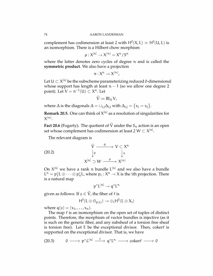
74 AARON LANDESMAN
complement has codimension at least 2 with H0(X,L) ' H0(U,L) isan isomorphism. There is a Hilbert chow morphism
ρ : X[n] → X(n) = Xn/Sn
where the latter denotes zero cycles of degree n and is called thesymmetric product. We also have a projection
π : Xn → X(n),
LetU ⊂ X[n] be the subscheme parameterizing reduced 0-dimensionalwhose support has length at least n− 1 (so we allow one degree 2point). Let V = π−1(U) ⊂ Xn. Let
V := Bl∆ V ,
where ∆ is the diagonals ∆ = ∪i,j∆i,j with ∆i,j =xi = xj
.
Remark 20.5. One can think of X[n] as a resolution of singularities forX(n).
Fact 20.6 (Fogarty). The quotient of V under the Sn action is an openset whose complement has codimension at least 2 W ⊂ X[n].
The relevant diagram is
(20.2)V V ⊂ Xn
X[n] ⊃W X(n)
q
p π
ρ
On X[n] we have a rank n bundle L[n] and we also have a bundleLn = p∗1L⊕ · · · ⊕ p∗nL, where pi : Xn → X is the ith projection. Thereis a natural map
p∗L[n] → q∗Ln
given as follows: If z ∈ V , the fiber of f is
H0(L⊗Op(z))→ ⊕iH0(L⊗ Xi)where q(z) = (x1, . . . , xn).
The map f is an isomorphism on the open set of tuples of distinctpoints. Therefore, the morphism of vector bundles is injective (as itis such on the generic fiber, and any subsheaf of a torsion free sheafis torsion free). Let E be the exceptional divisor. Then, cokerf issupported on the exceptional divisor. That is, we have
(20.3) 0 p∗L[n] q∗Ln cokerf 0f
MATH 245 NOTES: SYZYGIES 75
It turns out that cokerf has rank 0 and is supported on E, and it turnsout that det cokerf ' OX(E). Therefore,
detp∗L[n] ' Ln(−E).
We have
H0(X[n], detL[n]) ' H0(W, detL[n])
' H0(V ,p∗ detL[n])Sn
' H0(q∗Ln(−E))Sn
⊂ H0(q∗Ln)Sn
' H0(V ,L[n])Sn
' H0(Xn,L[n])Sn
Summarizing, we have a map
H0(X[n], detL[n])→ H0(Xn,Ln)Sn .
For σ ∈ Sn and ti ∈ H0(X,L), we define
σ (p∗1t1 ⊗ p∗2t2 ⊗ · · · ⊗ p∗ntn) := sgn(σ)(p∗1tσ(1) ⊗ · · · p∗ntσ(n)
).
That is, Sn acts by permuting factors and taking determinants. There-fore,
H0(Xn,Ln)Sn ' ∧nH0(X,L).
Exercise 20.7. Verify that this construction is inverse to the map inthe other direction, yielding an isomorphism.
21. 6/5/17
Today, we’ll start by discussing Curvilinear schemes.
Definition 21.1. We say [Z] ⊂ X[n] is called curvilinear if
OZ,p ' C[t]/(t`).
The value of this concept of curvilinear schemes is that if we fixx ∈ Supp(Z), we can then define the residual of x for any curvilinearscheme.
76 AARON LANDESMAN
Definition 21.2. For Z a curvilinear scheme and x ∈ Supp(Z), theresidual τx is
τx(z) :=
Zy if y 6= xSpec C[t]/(t` − 1) if y = x
Exercise 21.3 (Easy exercise). Let X be a surface. The set of curvilin-ear schemes X[n]
curv ⊂ X[n] is open and its complement has codimen-sion 2.
Let
Zn ⊂ X[n]curv × X
be the universal subscheme. We have the residual morphism
τ : Zn → X[n−1]curv × X
([Z], x) 7→ (τx[Z], x)
The point of this is that it gives you inductive arguments.
Theorem 21.4 (Voisin). Let
(21.1)Zn X
[n]curv
X.
q
p
Let L be a line bundle on X. There is an isomorphism
Kn−1,1(X,L) ' H0(Zn,q∗ detL[n]
)/q∗H0
(X[n]curv, detL[n]
).
Proof. Recall last class we showed H0(detL[n]) = ∧nH0(X,L). Wehave
(21.2)X[n]curv × X X
X[n]curv
p2
p1
There is a morphism
φ : q∗L[n] → τ∗(p∗1L
[n−1] ⊕ p∗2L)
.
This map sends [Z] ∈ Zn for
τ(Z) =(Z ′, x
)
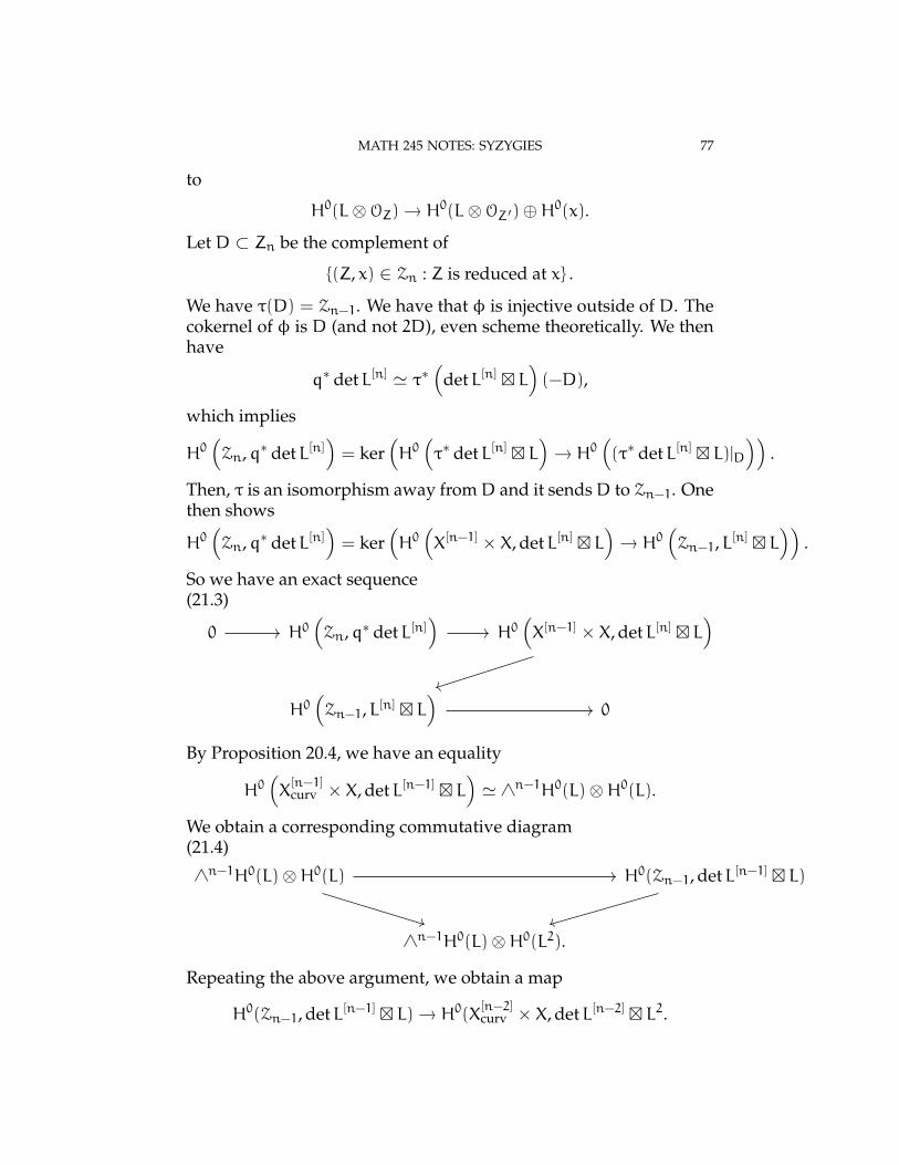
MATH 245 NOTES: SYZYGIES 77
to
H0(L⊗OZ)→ H0(L⊗OZ ′)⊕H0(x).
Let D ⊂ Zn be the complement of
(Z, x) ∈ Zn : Z is reduced at x .
We have τ(D) = Zn−1. We have that φ is injective outside of D. Thecokernel of φ is D (and not 2D), even scheme theoretically. We thenhave
q∗ detL[n] ' τ∗(
detL[n] L)(−D),
which implies
H0(Zn,q∗ detL[n]
)= ker
(H0(τ∗ detL[n] L
)→ H0((τ∗ detL[n] L)|D
)).
Then, τ is an isomorphism away fromD and it sendsD to Zn−1. Onethen shows
H0(Zn,q∗ detL[n]
)= ker
(H0(X[n−1] × X, detL[n] L
)→ H0(Zn−1,L[n] L
)).
So we have an exact sequence(21.3)
0 H0(Zn,q∗ detL[n]
)H0(X[n−1] × X, detL[n] L
)
H0(Zn−1,L[n] L
)0
By Proposition 20.4, we have an equality
H0(X[n−1]curv × X, detL[n−1] L
)' ∧n−1H0(L)⊗H0(L).
We obtain a corresponding commutative diagram(21.4)
∧n−1H0(L)⊗H0(L) H0(Zn−1, detL[n−1] L)
∧n−1H0(L)⊗H0(L2).
Repeating the above argument, we obtain a map
H0(Zn−1, detL[n−1] L)→ H0(X[n−2]curv × X, detL[n−2] L2.
78 AARON LANDESMAN
We similarly obtain
(21.5)
∧n−2H0(L)
H0(Zn,q∗ detL[n]) ∧n−1H0(L)⊗H0(L)
H0(Zn−1, detL[n−1] L)
∧n−2H0(L)⊗H0(L2)
δ
δ
We can identify
ker(∧n−1H0(X,L)⊗H0(L) δ−→ ∧n−2H0(L)⊗H0(L2)
)with
H0(Zn,q∗ detL[n]).
and im δn−2 ' q∗H0(X[n]curv × X, detL[n]).
Theorem 21.5 (Voisin). Let X be a K3 surface and L and ample line bun-dle. Suppose PicX ' ZL. We have L2 = 2g− 2, and assume g = 2− k.Then, Kk−1,1(C,ωC) = Kk−1,1(X,L) = 0 for C ∈ |L|.
By Lazarsfeld’s result, if C ∈ |L| is general, then it is Brill Noethergeneral for Gon(C) = k+ 1.
22. 6/7/17
Theorem 22.1 (Voisin). LetX be a K3 surface, L a line bundle and PicX 'ZL. We have L2 = 2g− 2 and g = 2k. Then, Kk,1(X,L) ' Kk,1(C,ωC) =0.
Remark 22.2. If C ∈ |L| is general then Lazarsfeld’s result says C isBrill-Noether-Petri general. We have
ρ(g, 1,k+ 1) = g− 2h1 = 2k− 2k = 0,
since 2− h1 = (k+ 1) + 1− 2k, so h1 = k. So, C has gonality k+ 1,by the Brill-Noether theorem.
MATH 245 NOTES: SYZYGIES 79
So, C carries a base point free D ∈ W1k+1. We have the Lazarsfeld-
Mukai bundle
(22.1) 0 F H0(C,D⊗OX i∗D 0.
We have that F has rank 2.
Lemma 22.3. If G is a vector bundle with the same Chern character of F,we have F ' G.
Proof. We showed previously
χ(F⊗ F∨) = 2− 2ρ(D) = 2.
Suppose G is any vector bundle with Ch(G) = Ch(F). Then,
χ(F⊗G∨) = 2,
since the Euler characteristic only depends on the Chern charac-ter, by Hirzebruch Riemann Roch. Then, either H0(F⊗ G∨) > 0 orH0(F∨ ⊗G) ' H2(F⊗G∨) > 0. Therefore, either there is a nonzeroG → F or F → G. But since F and F∨ are stable, and µ1(F) = µ1(G)and F is stable, we have seen F ' G.
22.1. An alternate construction of F. Using Lemma 22.3, we cannow give an alternate construction. The following construction iseither due to Serre or Griffiths-Harris.
Let D ∈W1k+1(C). We have
χ (OC(D)) = k+ 1+ 1− 2k = 2− k.
We know
h0 (OC(D)) = 2,
so
h0(ωC −D) = h1 (O(D)) = k.
We have an exact sequence
(22.2) 0 O(−D) OC OD 0
which we twist to
(22.3) 0 ωC −D ωC ωC|D 0
Note thatωC|D ' OD. We obtain
h0(ωC) = 2k,h0 (ωC|C) = k+ 1.
80 AARON LANDESMAN
Chasing the exact sequences and using Riemann Roch, we deduce
H0(C,ωC)→ H0(D,ωC|D)
has 1-dimensional cokernel.On a K3 surface, we have the sequence
(22.4) 0 OX L L|C 0
where L|C ' ωC. We have h1(OX) = 0. Therefore
(22.5)
H0(X,L) H0(C,ωC)
H0(D,ωC|D)
f
Note that f has corank 1 if and only ifD ∈Wk+1 withD ∈ Pick+1(C).Look at the ideal sheaf of D as a codimension 2 subscheme of X. Wehave the sequence
(22.6) 0 ID OX OD 0
We have the following facts:
Fact 22.4. (1) Ext1(OD,L∨) = 0(2) Ext2(OD,L∨) ' H0(L∨⊗OD), thinking of the latter as a vector
space.
To prove the above facts, use the local to global Ext sequence.We now apply the functorHom
(•,L∨
)to the prior exact sequences.
We obtain(22.7)
0 Ext1(OX,L∨) Ext1(ID,L∨) H0(L∨ ⊗OD) Ext2(O,L∨).
Using the facts, we obtain(22.8)
0 H1(L∨) Ext1(ID,L∨) H0(L∨ ⊗OD) H0(L)∨,
where we used
Ext2(O,L∨) = H2(L∨) = H0(L)∨.
Dualizing the above sequence, we obtain(22.9)
H0(L) H0(L⊗OD) Ext1(ID,L∨)∨ H1(L) 0.resD
MATH 245 NOTES: SYZYGIES 81
We have shown resD is not surjective with corank 1 if and only ifD ∈W1
k+1. If D ∈W1k+1, we get
0 6= e ∈ Ext1(ID,L∨)∨
' Ext1(ID ⊗ L,ωX)∨
Therefore,
e∨ ∈ Ext1(ID ⊗ L,OX)
This element corresponds to an extension
(22.10) 0 OX V ID ⊗ L 0.
Let E := F∨. Via a local computation, one obtains that V is a vectorbundle with ChV = Ch(F∨) = Ch(E). So, V ' E ' F∨, usingLemma 22.3.
Note that our construction in this case yields
(22.11) 0 OX E ID ⊗ L 0.s
We then obtain a global section s of E vanishing on D ∈ W1k+1. It
follows that the map E → ID ⊗ L can be written as ∧s (sending t 7→t∧ s). So the exact sequence above is
(22.12) 0 OX E ID ⊗ L 0.s ∧s
For any t ∈ H0(E), we can see that V(t) is some W1k+1(C
′) for someC ′.
Motivated by the above description, Voisin studies
φ : P(H0(E)
)→ X[k+1]
s 7→ V(s).
One can verify φ is a closed immersion. Let’s use this an Voisin’sdescription of syzygies via the Hilbert scheme.
Define
P(H0(E)
)curv
:= P(H0(E)
)∩ X[k+1]
curv .
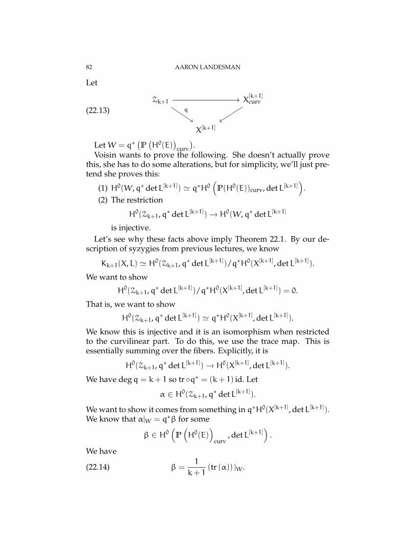
82 AARON LANDESMAN
Let
(22.13)Zk+1 X
[k+1]curv
X[k+1]
q
LetW = q∗(P(H0(E)
)curv
).
Voisin wants to prove the following. She doesn’t actually provethis, she has to do some alterations, but for simplicity, we’ll just pre-tend she proves this:
(1) H0(W,q∗ detL[k+1]) ' q∗H0(
P(H0(E))curv, detL[k+1])
.(2) The restriction
H0(Zk+1,q∗ detL[k+1])→ H0(W,q∗ detL[k+1]
is injective.Let’s see why these facts above imply Theorem 22.1. By our de-
scription of syzygies from previous lectures, we know
Kk+1(X,L) ' H0(Zk+1,q∗ detL[k+1])/q∗H0(X[k+1], detL[k+1]).
We want to show
H0(Zk+1,q∗ detL[k+1])/q∗H0(X[k+1], detL[k+1]) = 0.
That is, we want to show
H0(Zk+1,q∗ detL[k+1]) ' q∗H0(X[k+1], detL[k+1]).
We know this is injective and it is an isomorphism when restrictedto the curvilinear part. To do this, we use the trace map. This isessentially summing over the fibers. Explicitly, it is
H0(Zk+1,q∗ detL[k+1])→ H0(X[k+1], detL[k+1]).
We have degq = k+ 1 so tr q∗ = (k+ 1) id. Let
α ∈ H0(Zk+1,q∗ detL[k+1]).
We want to show it comes from something in q∗H0(X[k+1], detL[k+1]).We know that α|W = q∗β for some
β ∈ H0(
P(H0(E)
)curv
, detL[k+1])
.
We have
(22.14) β =1
k+ 1(tr (α)) |W .
MATH 245 NOTES: SYZYGIES 83
If α ′ = α− q∗(1k+1 tr(α)
). We have by (22.14), that α ′|W = 0. The
second property (saying that the restriction to W is injective). Weobtain α ′ = 0 so α ∈ im q∗ as we wanted, completing the proof.


![[David Eisenbud] the Geometry of Syzygies(BookFi.org)](https://img.pdfslide.us/doc/110x75/55cf9ce3550346d033ab69fe/david-eisenbud-the-geometry-of-syzygiesbookfiorg.jpg)
