Embed Size (px)
DESCRIPTION
Math 144. Confidence Interval. In addition to the estimated value of the estimator, some statisticians suggest that we should also consider the variance of the estimator. - PowerPoint PPT Presentation
Citation preview
Math 144
Confidence Interval
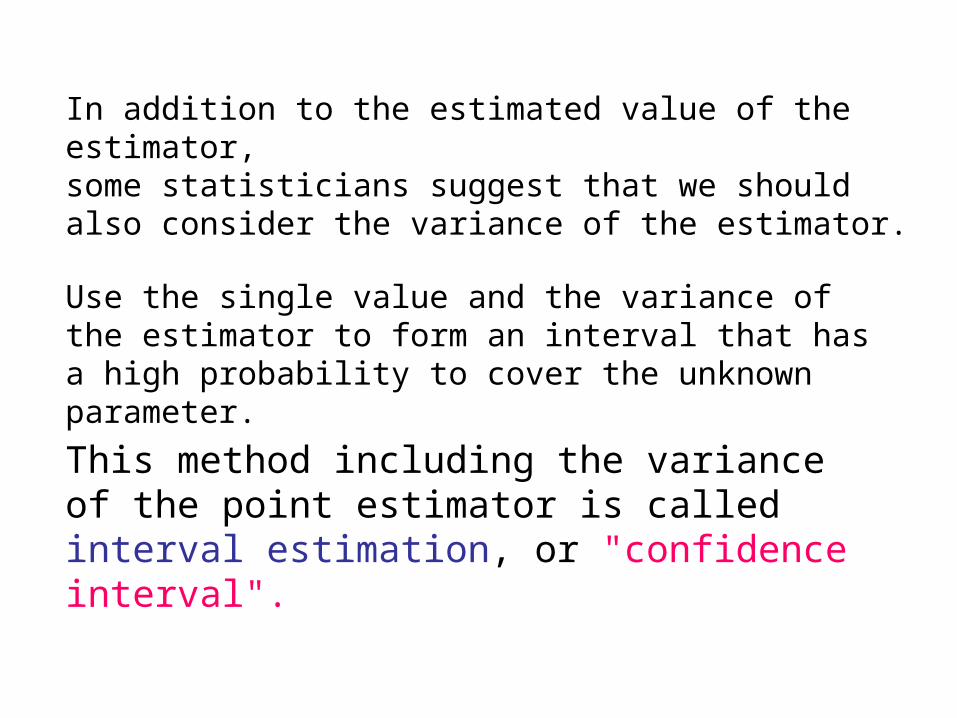
In addition to the estimated value of the estimator, some statisticians suggest that we should also consider the variance of the estimator.
Use the single value and the variance of the estimator to form an interval that has a high probability to cover the unknown parameter.
This method including the variance of the point estimator is called interval estimation, or "confidence interval".
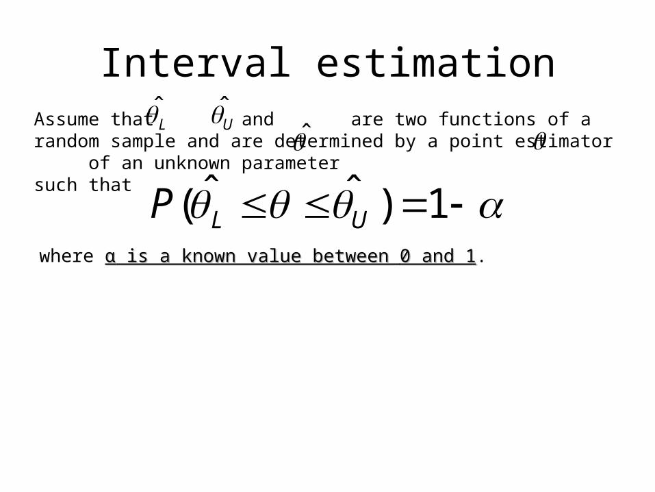
Interval estimationAssume that and are two functions of a random sample and are determined by a point estimator of an unknown parameter such that
L U
where αα is a known value between is a known value between 0 and 10 and 1.
1)ˆˆ( ULP
Interval estimation
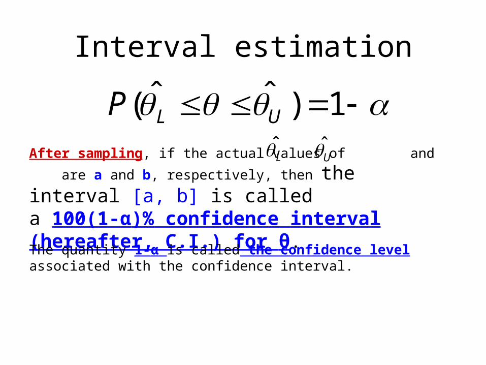
After sampling, if the actual values of and are a and b,
respectively, then the interval [a, b] is called a 100(1-α)% confidence interval (hereafter, C.I.) for θ.
L U
The quantity 1-α is called the confidence level associated with the confidence interval.
1)ˆˆ( ULP
Caution:
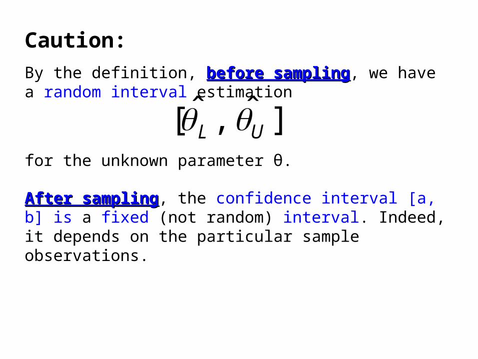
After samplingAfter sampling, the confidence interval [a, b] is a fixed (not random) interval. Indeed, it depends on the particular sample observations.
By the definition, before samplingbefore sampling, we have a random interval estimation
]ˆ,ˆ[ UL for the unknown parameter θ.
Caution:
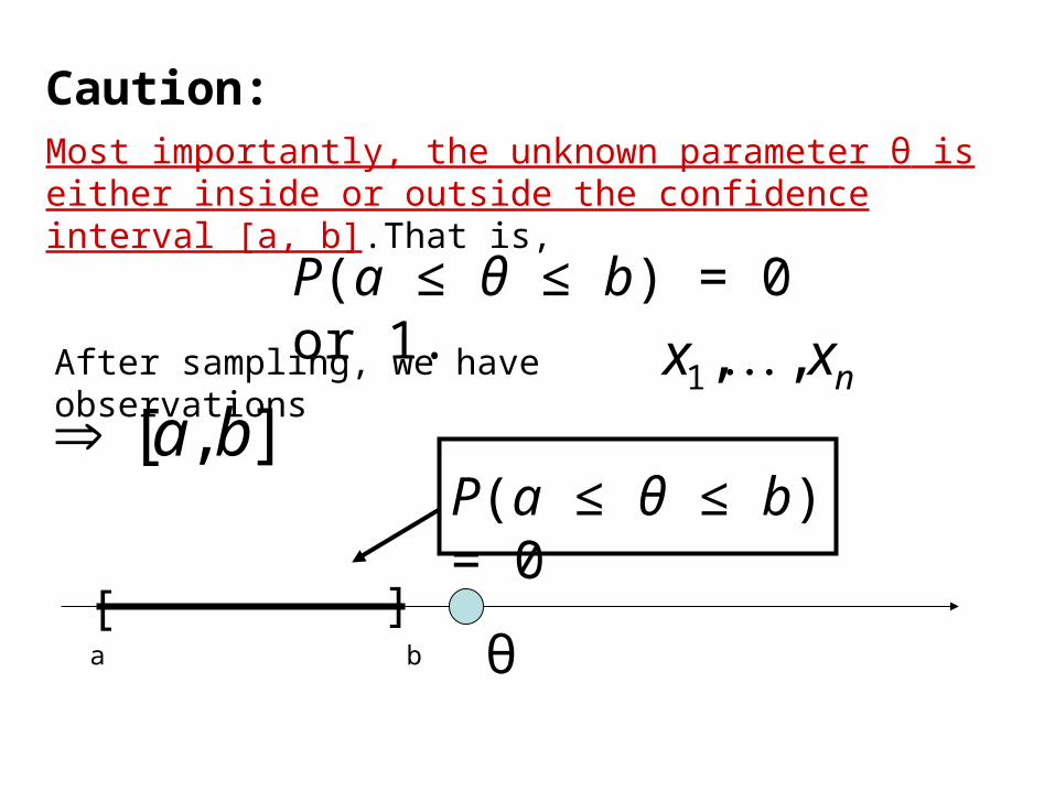
Most importantly, the unknown parameter θ is either inside or outside the confidence interval [a, b].That is,
P(a ≤ θ ≤ b) = 0 or 1.
θ
After sampling, we have observations nxx ,,1 ],[ ba
[
[
a b
P(a ≤ θ ≤ b) = 0
Caution:
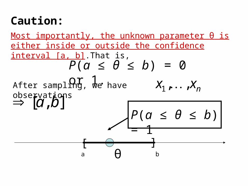
Most importantly, the unknown parameter θ is either inside or outside the confidence interval [a, b].That is,
P(a ≤ θ ≤ b) = 0 or 1.
θ
After sampling, we have observations nxx ,,1 ],[ ba
[
[
a b
P(a ≤ θ ≤ b) = 1
Caution:
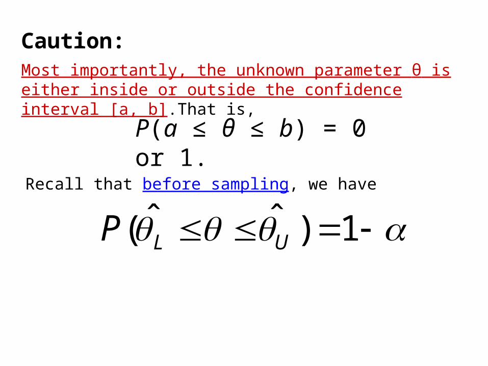
Most importantly, the unknown parameter θ is either inside or outside the confidence interval [a, b].That is,
P(a ≤ θ ≤ b) = 0 or 1.
Recall that before sampling, we have
1)ˆˆ( ULP
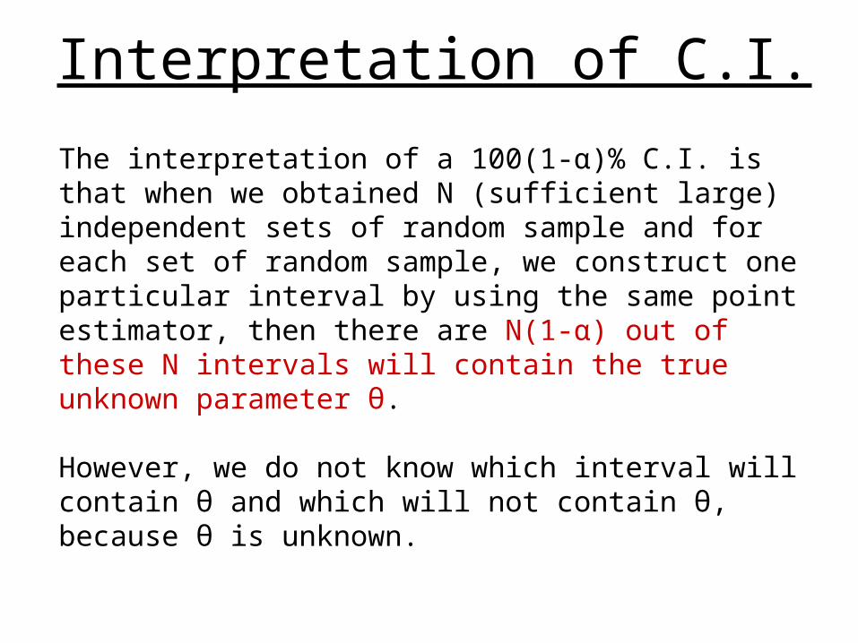
The interpretation of a 100(1-α)% C.I. is that when we obtained N (sufficient large) independent sets of random sample and for each set of random sample, we construct one particular interval by using the same point estimator, then there are N(1-α) out of these N intervals will contain the true unknown parameter θ.
However, we do not know which interval will contain θ and which will not contain θ, because θ is unknown.
Interpretation of C.I.
Interpretation of C.I.
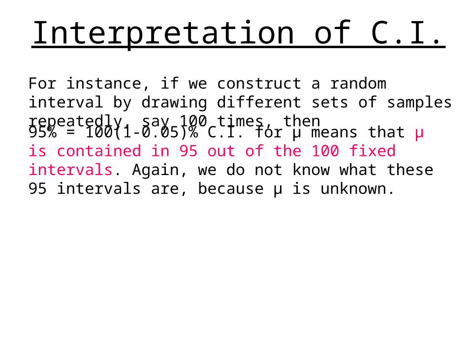
For instance, if we construct a random interval by drawing different sets of samples repeatedly, say 100 times, then
95% = 100(1-0.05)% C.I. for μ means that μ is contained in 95 out of the 100 fixed intervals. Again, we do not know what these 95 intervals are, because µ is unknown.
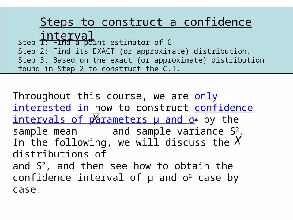
Throughout this course, we are only interested in how to construct confidence intervals of parameters µ and σ2 by the sample mean and sample variance S2. X
In the following, we will discuss the distributions ofand S2, and then see how to obtain the confidence interval of µ and σ2 case by case.
X
Step 1: Find a point estimator of θStep 2: Find its EXACT (or approximate) distribution. Step 3: Based on the exact (or approximate) distribution found in Step 2 to construct the C.I.
Steps to construct a confidence interval
One sample
Confidence Interval for µ with NORMAL population
(known variance)
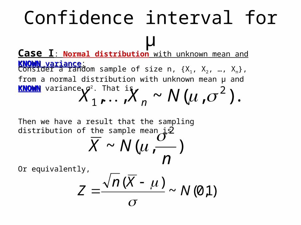
Confidence interval for µCase I: Normal distribution with unknown mean and KNOWNKNOWN variance variance:
Consider a random sample of size n, {X1, X2, …, Xn}, from a normal distribution with unknown mean µ and KNOWNKNOWN variance σ2. That is,
.),(~,, 21 NXX n
Then we have a result that the sampling distribution of the sample mean is
),(~2
nNX
)1,0(~)(N
XnZ
Or equivalently,
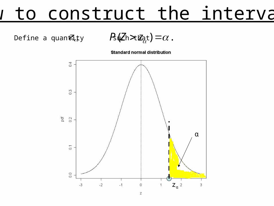
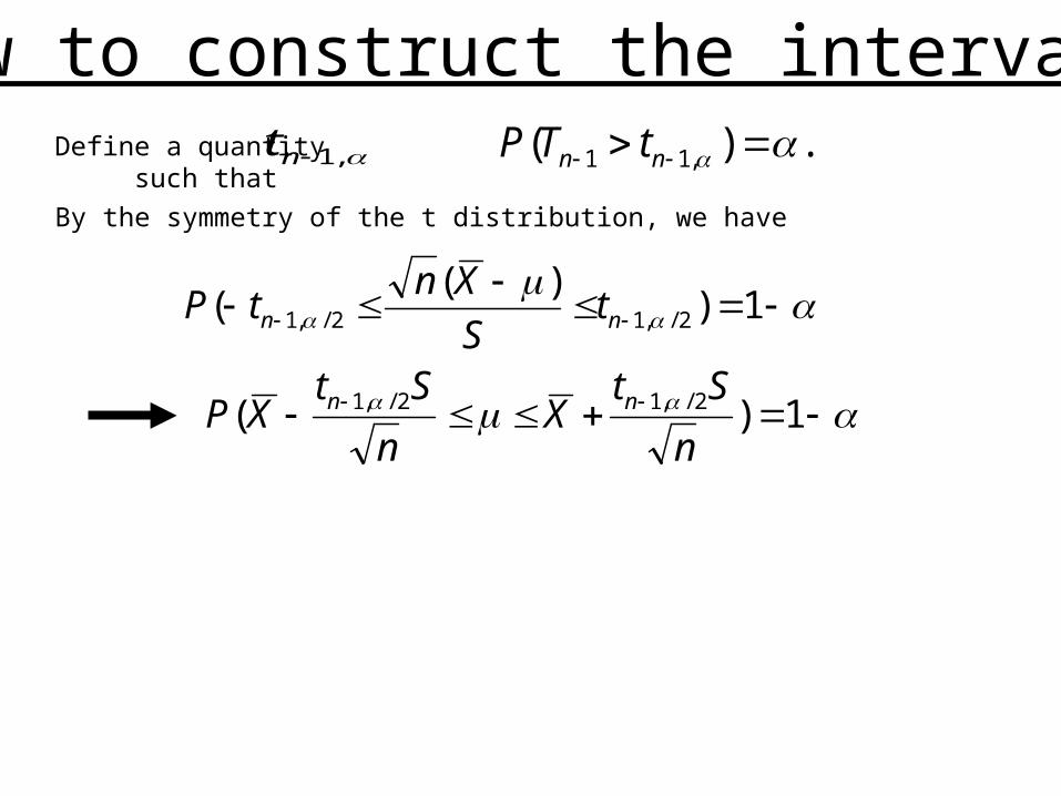
How to construct the interval?zDefine a quantity such that .)( zZP
zα
α
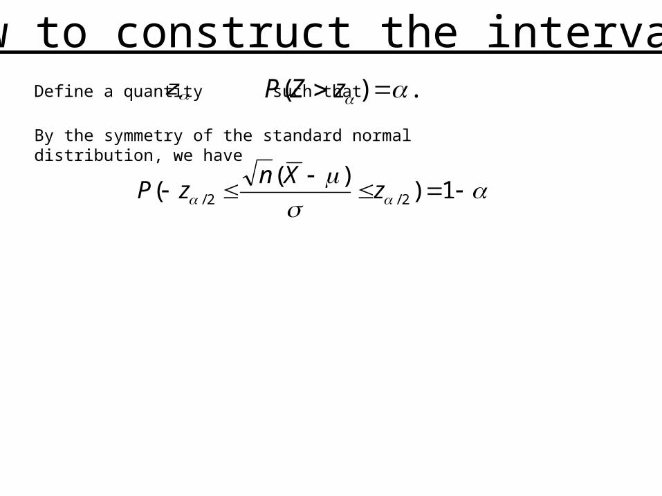
How to construct the interval?zDefine a quantity such that .)( zZP
1)
)(( 2/2/ z
XnzP
By the symmetry of the standard normal distribution, we have
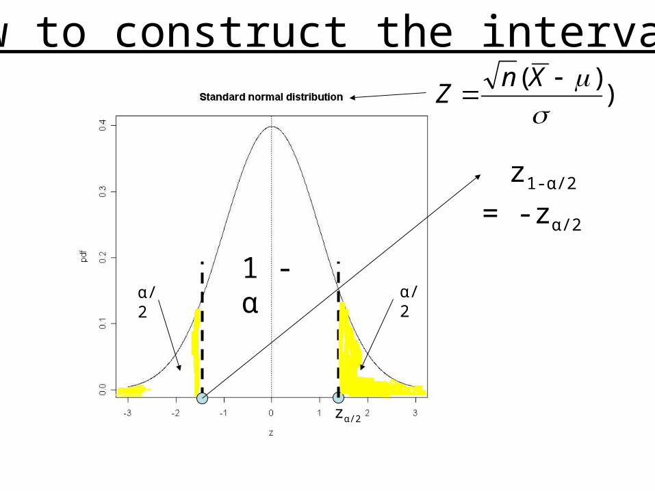
How to construct the interval?
zα/2
α/2
z1-α/2
α/2
))(
Xn
Z
1 - α
= -zα/2
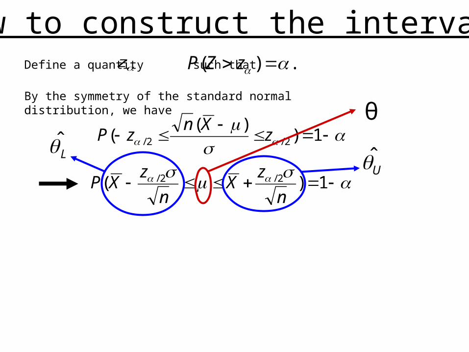
How to construct the interval?zDefine a quantity such that .)( zZP
1)
)(( 2/2/ z
XnzP
By the symmetry of the standard normal distribution, we have
1)( 2/2/
n
zX
n
zXP
θ
LU
How to construct the interval?
n
zx
n
zx
2/2/ ,
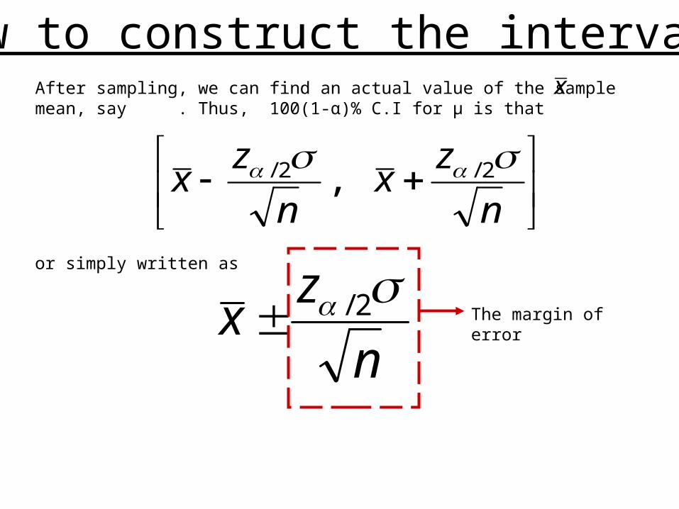
xAfter sampling, we can find an actual value of the sample mean, say . Thus, 100(1-α)% C.I for μ is that
or simply written as
n
zx
2/ The margin of error
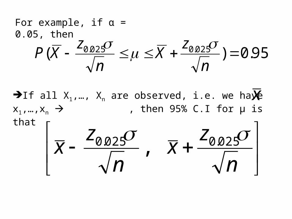
xIf all X1,…, Xn are observed, i.e. we have x1,…,xn , then 95% C.I for μ is that
n
zx
n
zx
025.0025.0 ,
95.0)( 025.0025.0 n
zX
n
zXP
For example, if α = 0.05, then
10)( 025.0025.0 orn
zx
n
zxP
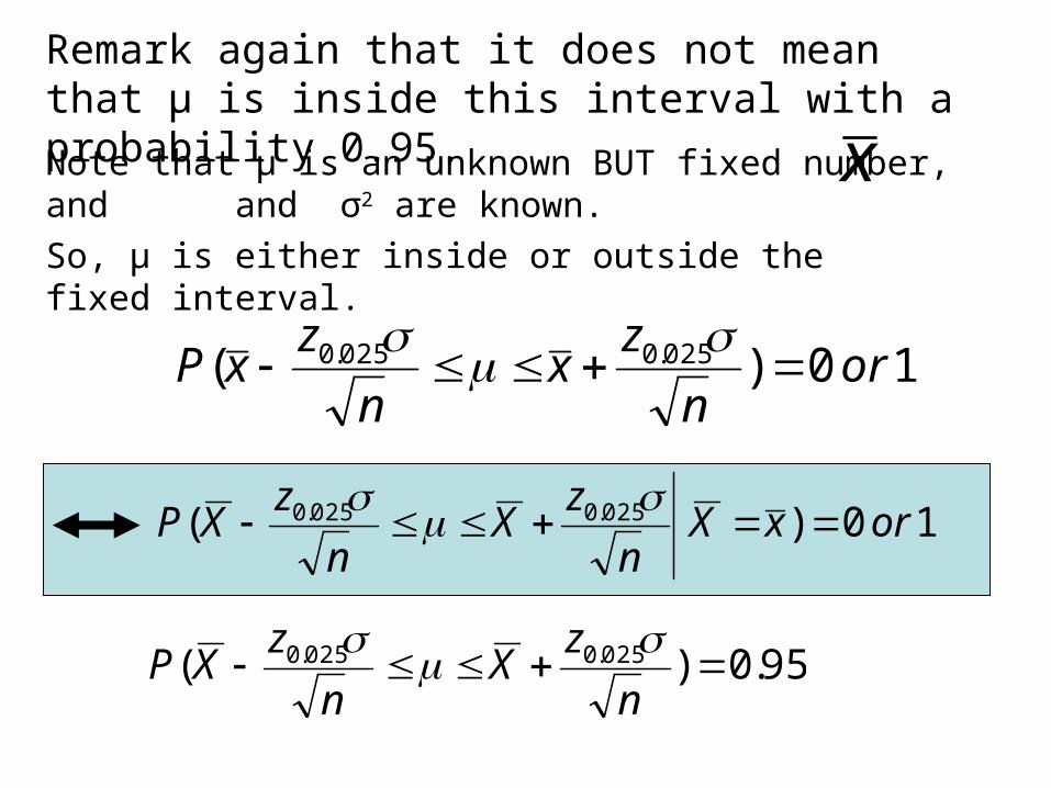
Remark again that it does not mean that μ is inside this interval with a probability 0.95.
So, μ is either inside or outside the fixed interval.
Note that μ is an unknown BUT fixed number, and and σ2 are known.
x
10)( 025.0025.0 orxXn
zX
n
zXP
95.0)( 025.0025.0 n
zX
n
zXP
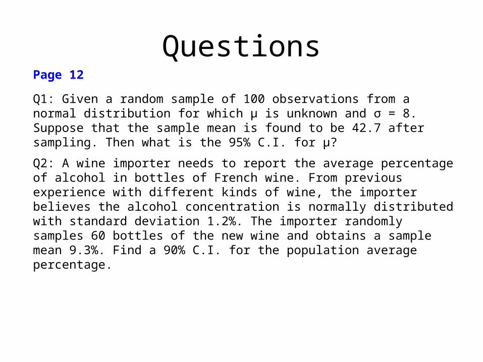
Questions
Q1: Given a random sample of 100 observations from a normal distribution for which µ is unknown and σ = 8. Suppose that the sample mean is found to be 42.7 after sampling. Then what is the 95% C.I. for µ?
Page 12
Q2: A wine importer needs to report the average percentage of alcohol in bottles of French wine. From previous experience with different kinds of wine, the importer believes the alcohol concentration is normally distributed with standard deviation 1.2%. The importer randomly samples 60 bottles of the new wine and obtains a sample mean 9.3%. Find a 90% C.I. for the population average percentage.

One sample
Confidence Interval for µ with NORMAL population
(unknown variance)
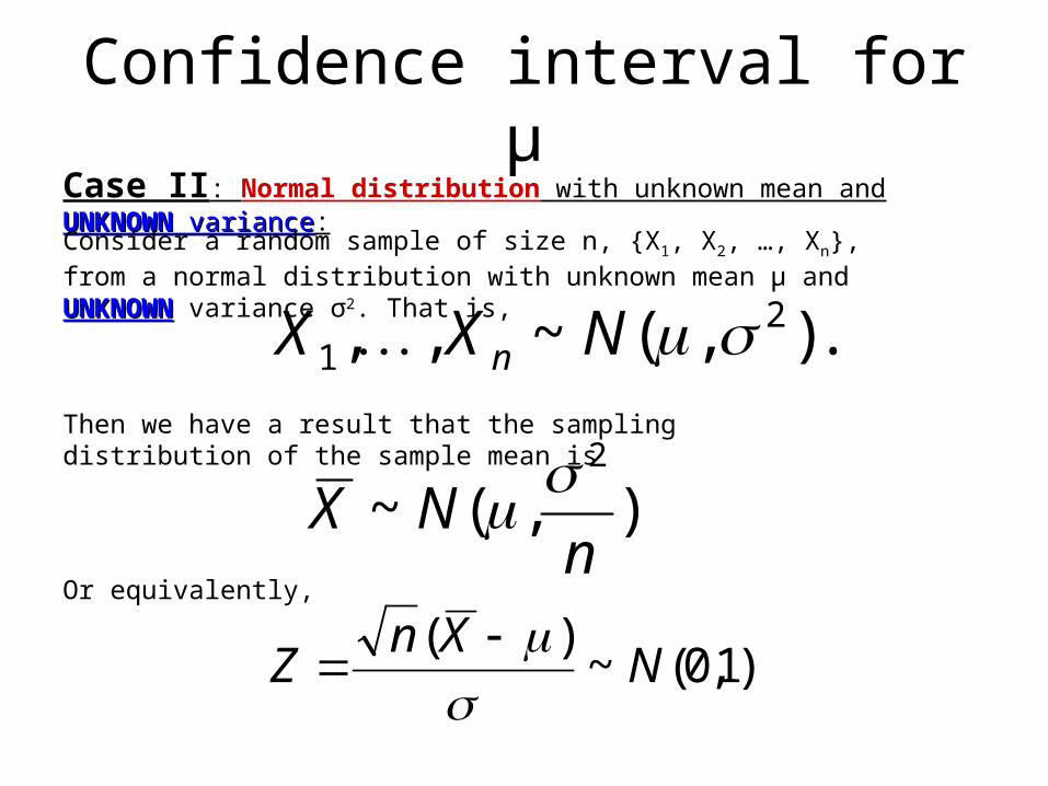
Confidence interval for µCase II: Normal distribution with unknown mean and UNKNOWNUNKNOWN variance variance:
Consider a random sample of size n, {X1, X2, …, Xn}, from a normal distribution with unknown mean µ and UNKNOWNUNKNOWN variance σ2. That is,
.),(~,, 21 NXX n
Then we have a result that the sampling distribution of the sample mean is
),(~2
nNX
)1,0(~)(N
XnZ
Or equivalently,
n
zx
n
zx
2/2/ ,
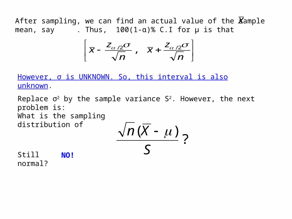
xAfter sampling, we can find an actual value of the sample mean, say . Thus, 100(1-α)% C.I for μ is that
However, σ is UNKNOWN. So, this interval is also unknown.
Replace σ2 by the sample variance S2. However, the next problem is:
?)(
S
Xn What is the sampling distribution of
Still normal? NO!
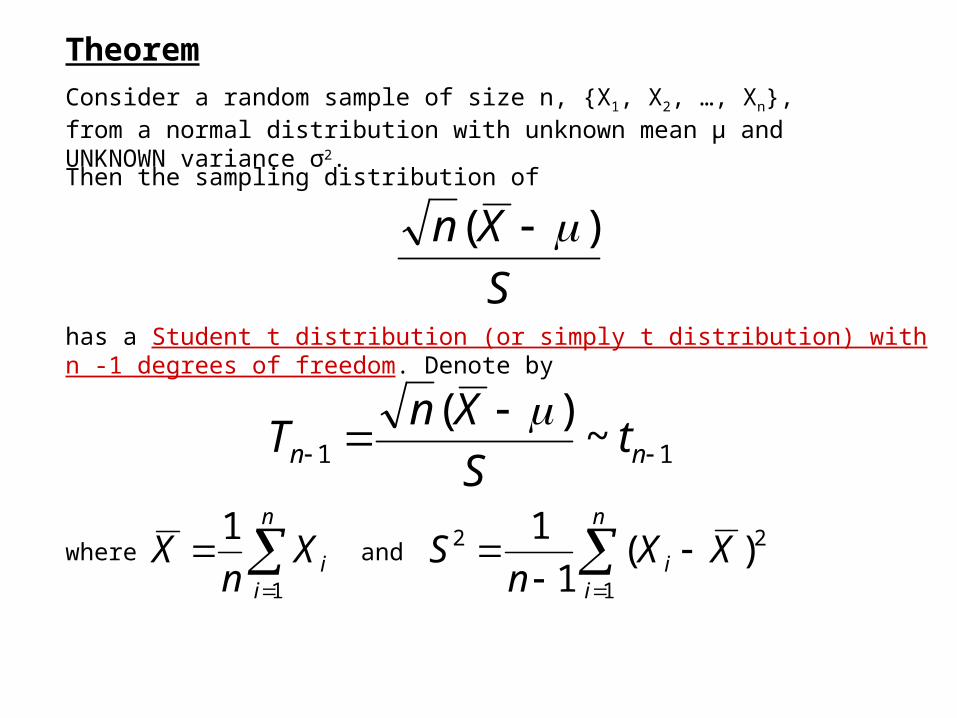
Consider a random sample of size n, {X1, X2, …, Xn}, from a normal distribution with unknown mean µ and UNKNOWN variance σ2.
Then the sampling distribution of
S
Xn )(
has a Student t distribution (or simply t distribution) with n -1 degrees of freedom. Denote by
11 ~)(
nn tS
XnT
n
iiXn
X1
1
n
ii XX
nS
1
22 )(1
1where and
Theorem
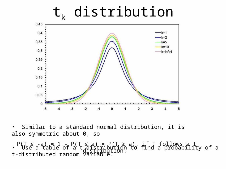
tk distribution
• Similar to a standard normal distribution, it is also symmetric about 0, so
P(T ≤ -a) = 1 - P(T ≤ a) = P(T ≥ a), if T follows a t distribution.
• Use a table of a t distribution to find a probability of a t-distributed random variable.
How to construct the interval?
1)
)(( 2/,12/,1 nn t
S
XntP
By the symmetry of the t distribution, we have
1)( 2/,12/,1
n
StX
n
StXP nn
,1nt .)( ,11 nn tTPDefine a quantity such that
How to construct the interval?
n
stx
n
stx nn 2/,12/,1 ,
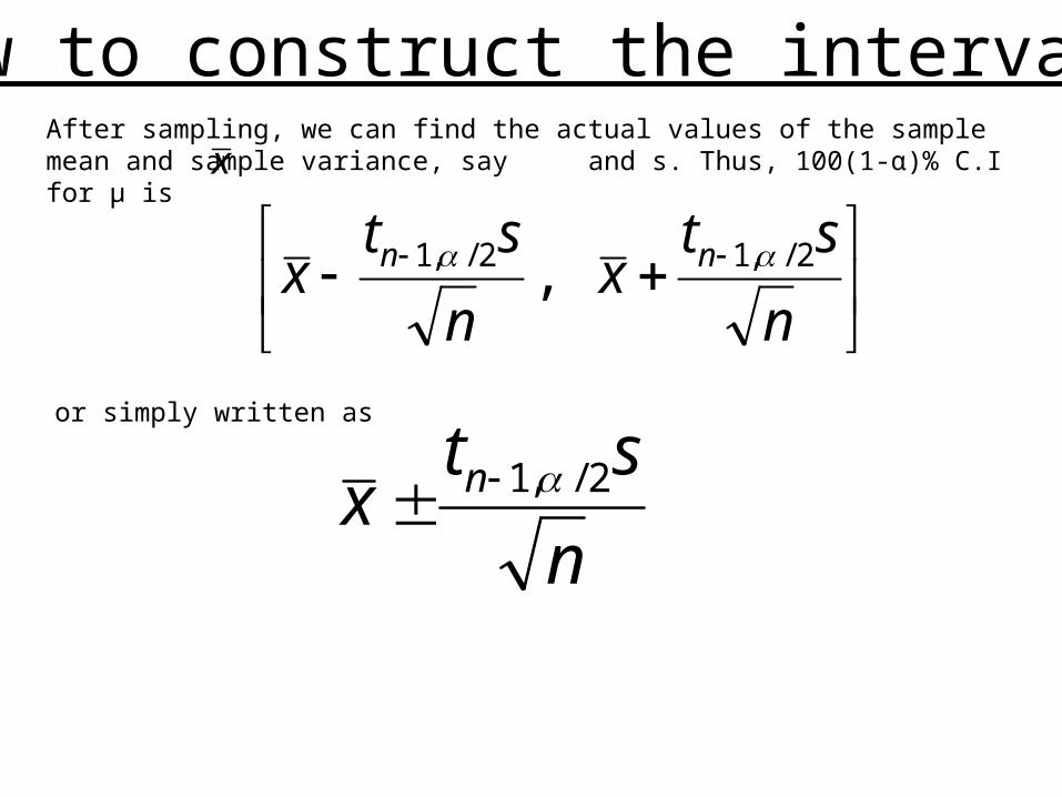
xAfter sampling, we can find the actual values of the sample mean and sample variance, say and s. Thus, 100(1-α)% C.I for μ is
or simply written as
n
stx n 2/,1
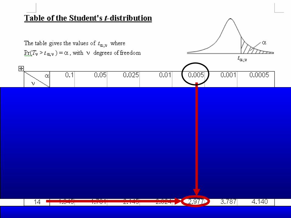
How to use the table of t distribution
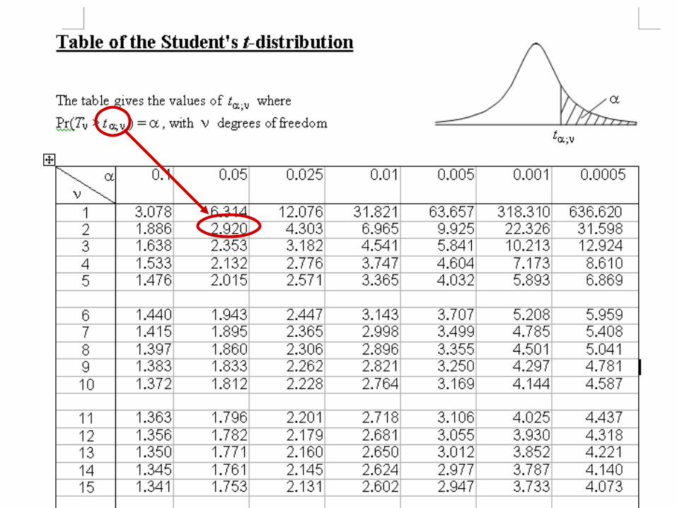
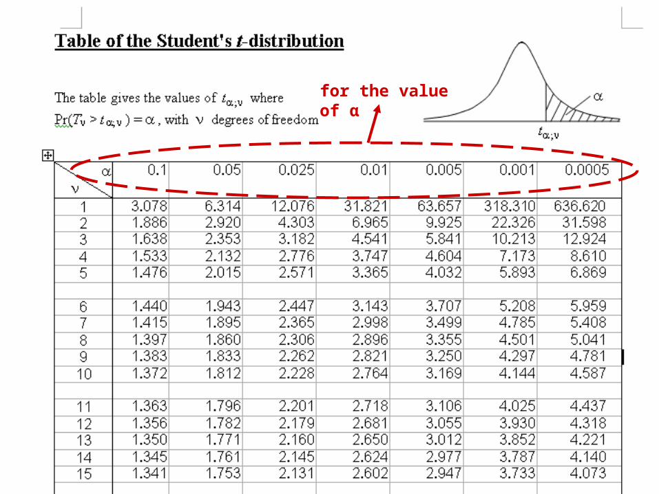
for the value of α
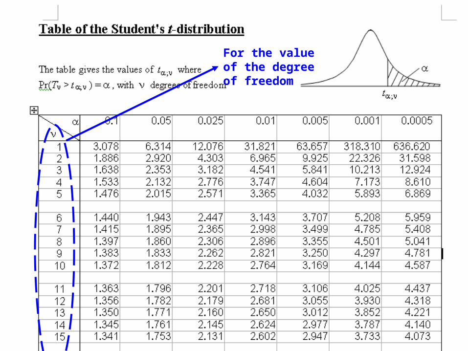
For the value of the degree of freedom
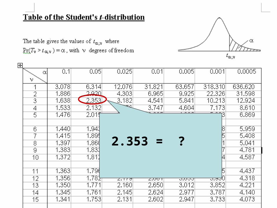
2.353 = ?
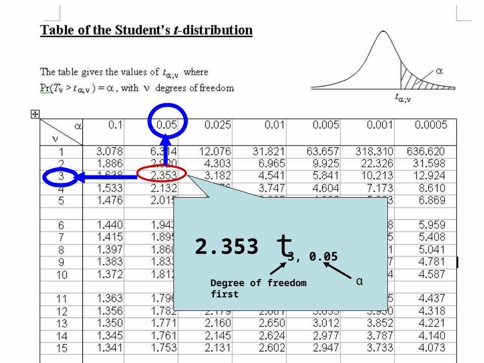
2.353 = ?t 3, 0.05
Degree of freedom first α
QuestionsPage 14 Q3
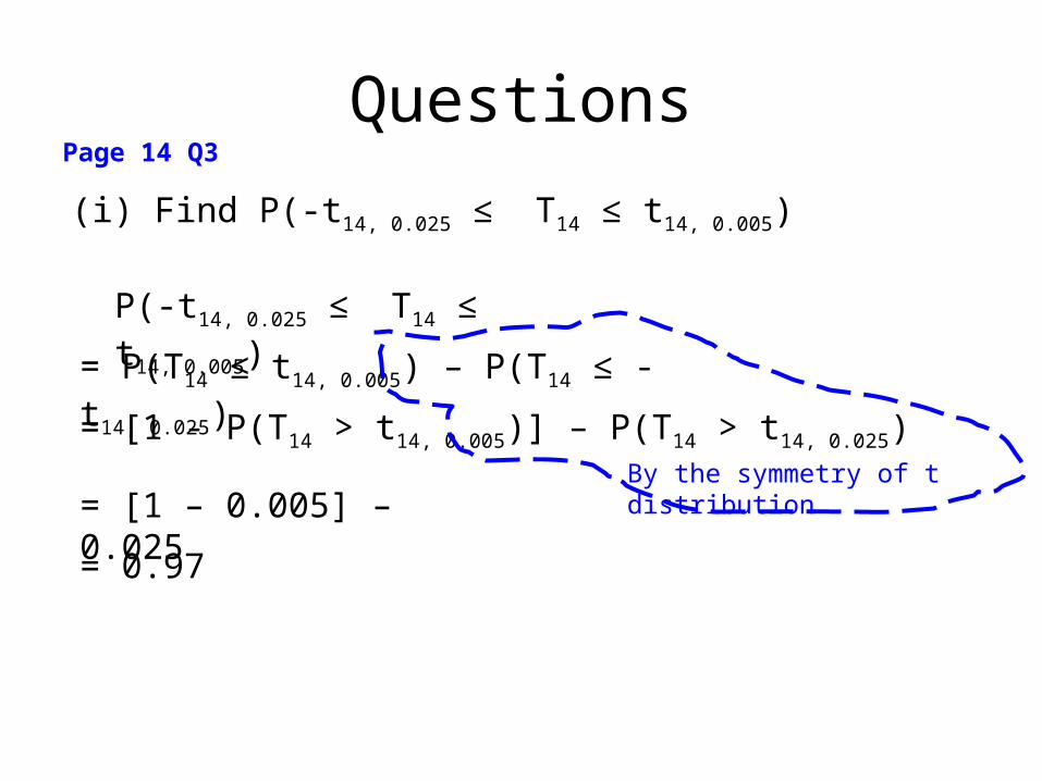
(i) Find P(-t14, 0.025 ≤ T14 ≤ t14, 0.005)
P(-t14, 0.025 ≤ T14 ≤ t14, 0.005)
= P(T14 ≤ t14, 0.005) – P(T14 ≤ -t14, 0.025)
= [1 - P(T14 > t14, 0.005)] – P(T14 > t14, 0.025)
= [1 – 0.005] – 0.025By the symmetry of t distribution
= 0.97
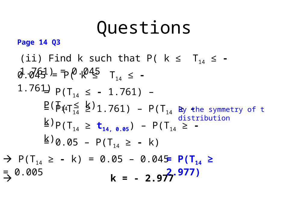
QuestionsPage 14 Q3
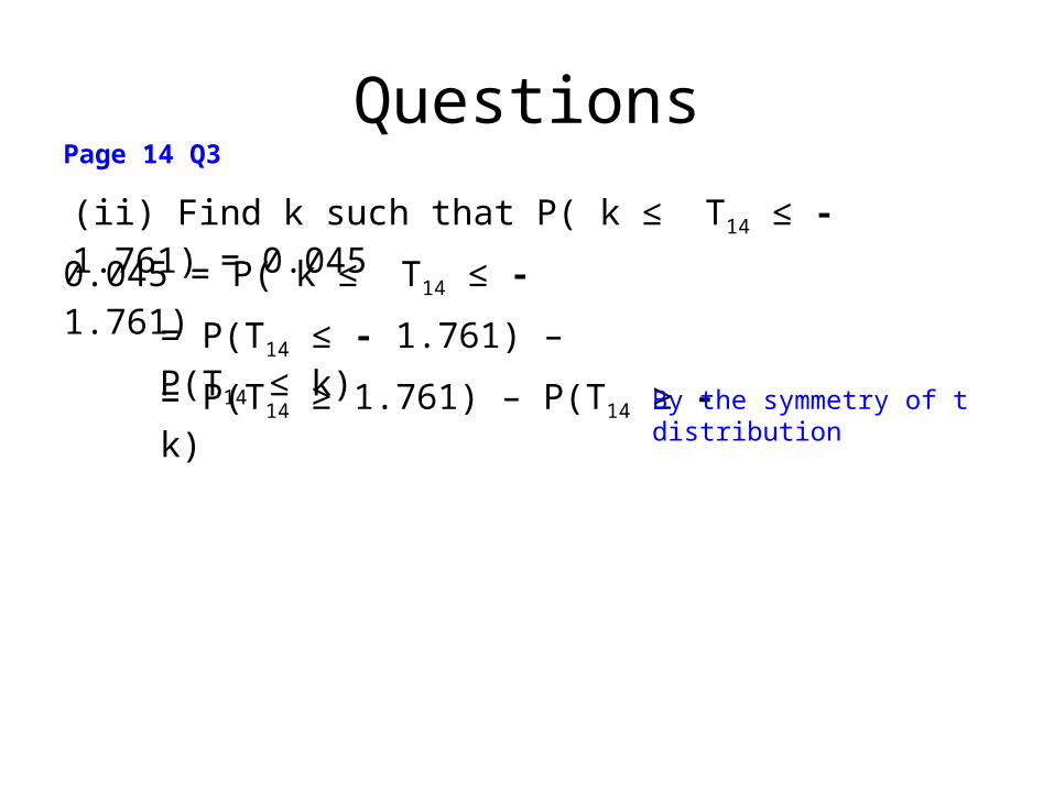
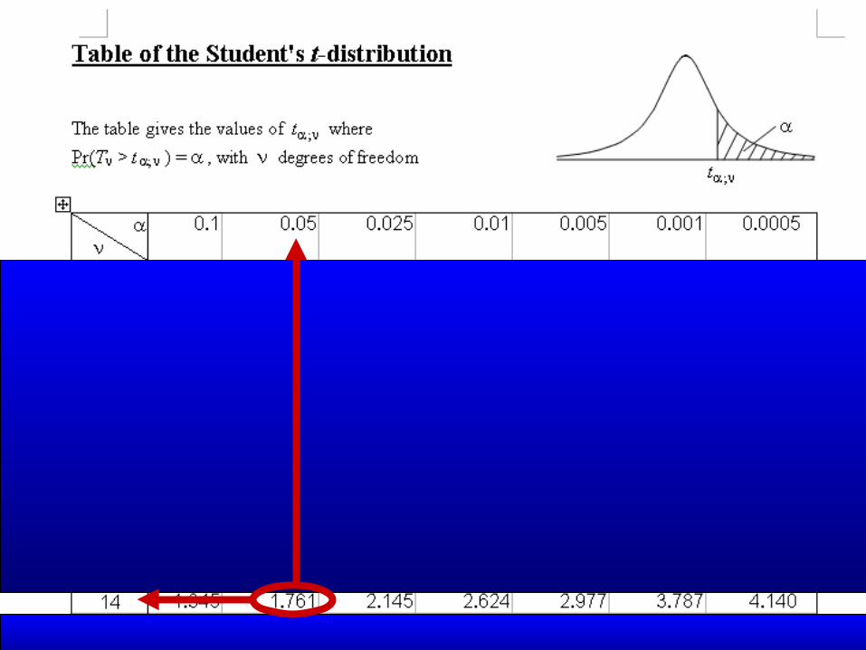
(ii) Find k such that P( k ≤ T14 ≤ - 1.761) = 0.045
0.045 = P( k ≤ T14 ≤ - 1.761)
= P(T14 ≤ - 1.761) – P(T14 ≤ k)
= P(T14 ≥ 1.761) – P(T14 ≥ - k) By the symmetry of t distribution
QuestionsPage 14 Q3
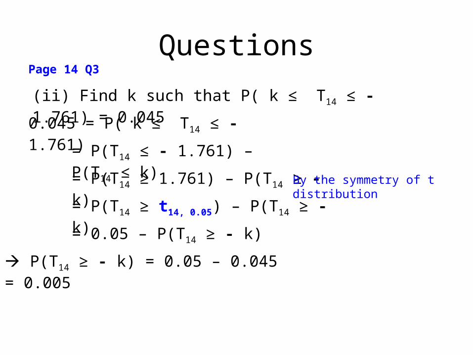
(ii) Find k such that P( k ≤ T14 ≤ - 1.761) = 0.045
0.045 = P( k ≤ T14 ≤ - 1.761)
= P(T14 ≤ - 1.761) – P(T14 ≤ k)
= P(T14 ≥ 1.761) – P(T14 ≥ - k) By the symmetry of t distribution
= P(T14 ≥ t14, 0.05) – P(T14 ≥ - k)
= 0.05 – P(T14 ≥ - k)
P(T14 ≥ - k) = 0.05 – 0.045 = 0.005
QuestionsPage 14 Q3
(ii) Find k such that P( k ≤ T14 ≤ - 1.761) = 0.045
0.045 = P( k ≤ T14 ≤ - 1.761)
= P(T14 ≤ - 1.761) – P(T14 ≤ k)
= P(T14 ≥ 1.761) – P(T14 ≥ - k) By the symmetry of t distribution
= P(T14 ≥ t14, 0.05) – P(T14 ≥ - k)
= 0.05 – P(T14 ≥ - k)
P(T14 ≥ - k) = 0.05 – 0.045 = 0.005 = P(T14 ≥ 2.977)
k = - 2.977
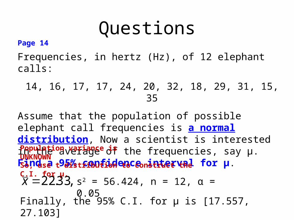
QuestionsPage 14
Frequencies, in hertz (Hz), of 12 elephant calls:
14, 16, 17, 17, 24, 20, 32, 18, 29, 31, 15, 35
Assume that the population of possible elephant call frequencies is a normal distribution, Now a scientist is interested in the average of the frequencies, say µ. Find a 95% confidence interval for µ.
Population variance is UNKNOWN
So, use t distribution to construct the C.I. for µ.
,33.22x s2 = 56.424, n = 12, α = 0.05
Finally, the 95% C.I. for µ is [17.557, 27.103]
Remark:
When n > 30, the difference of a t distribution with n -1 degrees of freedom and the standard normal distribution is small. So, we have
.2/2/,1 ztn
Therefore, we can use
n
szx
n
szx 2/2/ ,
to approximate the 100(1-α)% C.I for μ with unknown variance, as n > 30.
Two samples
Confidence Interval for µX - µY with NORMAL populations
(known variances)
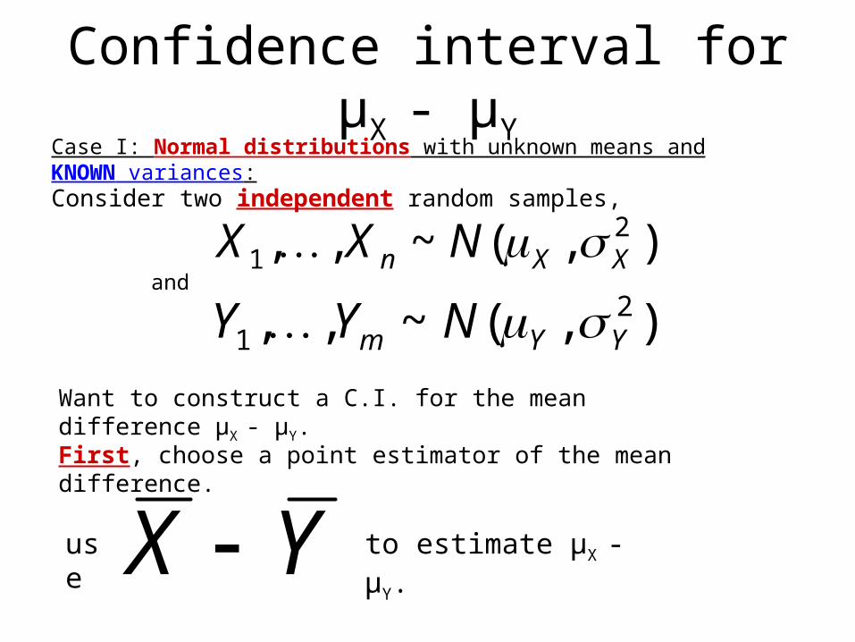
Confidence interval for µX - µY
Case I: Normal distributions with unknown means and KNOWN variances:
Consider two independent random samples,
),(~,, 21 XXn NXX
),(~,, 21 YYm NYY
and
Want to construct a C.I. for the mean difference µX - µY.
First, choose a point estimator of the mean difference.
YX use to estimate µX - µY.
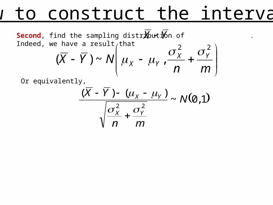
How to construct the interval?Second, find the sampling distribution of . Indeed, we have a result that YX
mn
NYX YXYX
22
,~)(
Or equivalently,
1,0~)()(
22N
mn
YX
YX
YX
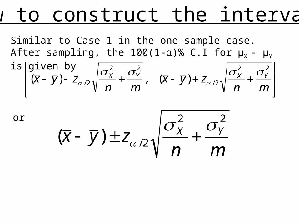
How to construct the interval?
mn
zyxmn
zyx YXYX22
2/
22
2/ )(,)(
Similar to Case 1 in the one-sample case. After sampling, the 100(1-α)% C.I for μX - μY is given by
mnzyx YX
22
2/)(
or
mn
zyxmn
zyx11
)(,11
)( 2/2/
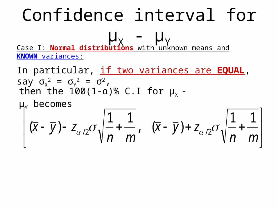
then the 100(1-α)% C.I for μX - μY becomes
Confidence interval for µX - µY
Case I: Normal distributions with unknown means and KNOWN variances:
In particular, if two variances are EQUAL, say σX2 = σY
2 = σ2,
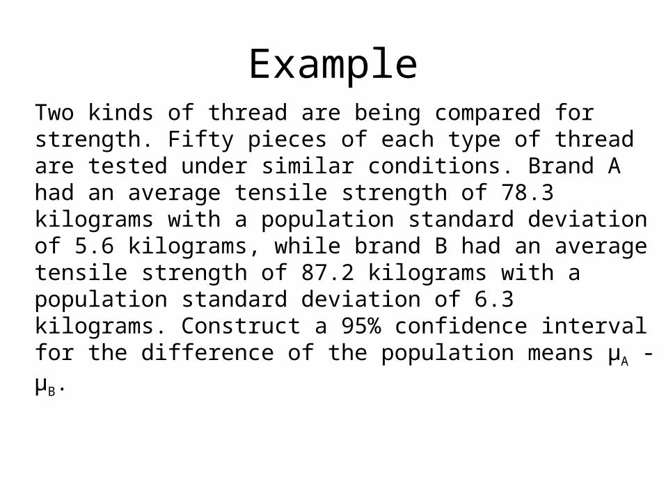
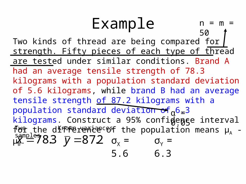
ExampleTwo kinds of thread are being compared for strength. Fifty pieces of each type of thread are tested under similar conditions. Brand A had an average tensile strength of 78.3 kilograms with a population standard deviation of 5.6 kilograms, while brand B had an average tensile strength of 87.2 kilograms with a population standard deviation of 6.3 kilograms. Construct a 95% confidence interval for the difference of the population means µA - µB.
ExampleTwo kinds of thread are being compared for strength. Fifty pieces of each type of thread are tested under similar conditions. Brand A had an average tensile strength of 78.3 kilograms with a population standard deviation of 5.6 kilograms, while brand B had an average tensile strength of 87.2 kilograms with a population standard deviation of 6.3 kilograms. Construct a 95% confidence interval for the difference of the population means µA - µB.
Two samples Known variances
3.78x 2.87y σX = 5.6 σY = 6.3
n = m = 50
α = 0.05
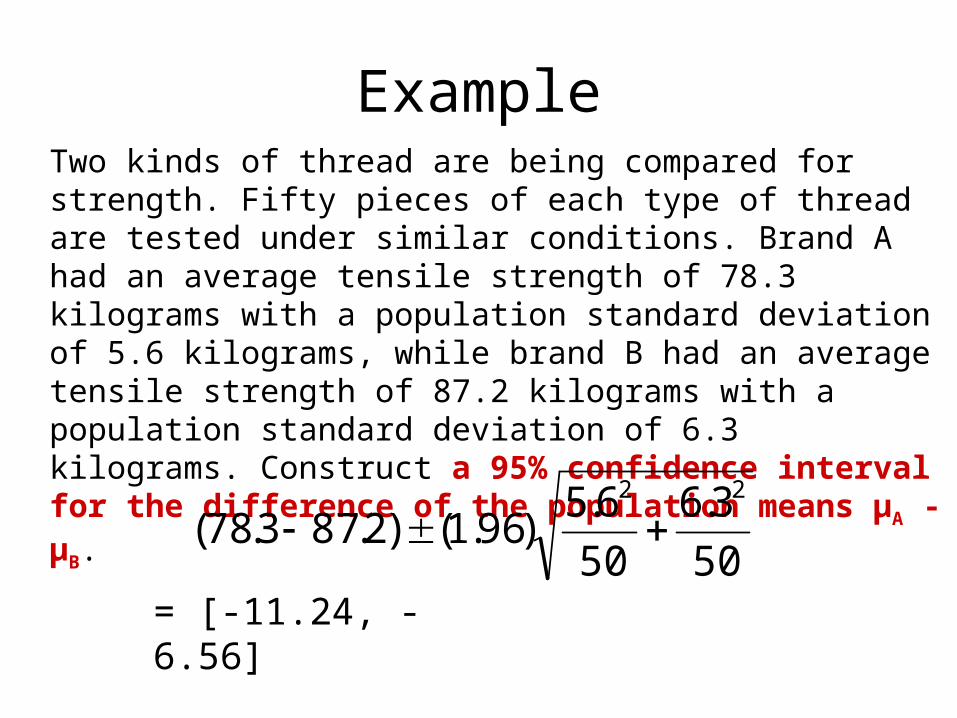
ExampleTwo kinds of thread are being compared for strength. Fifty pieces of each type of thread are tested under similar conditions. Brand A had an average tensile strength of 78.3 kilograms with a population standard deviation of 5.6 kilograms, while brand B had an average tensile strength of 87.2 kilograms with a population standard deviation of 6.3 kilograms. Construct a 95% confidence interval for the difference of the population means µA - µB.
50
3.6
50
6.5)96.1()2.873.78(
22
= [-11.24, -6.56]
Two samples
Confidence Interval for µX - µY with NORMAL populations
(unknown variances)
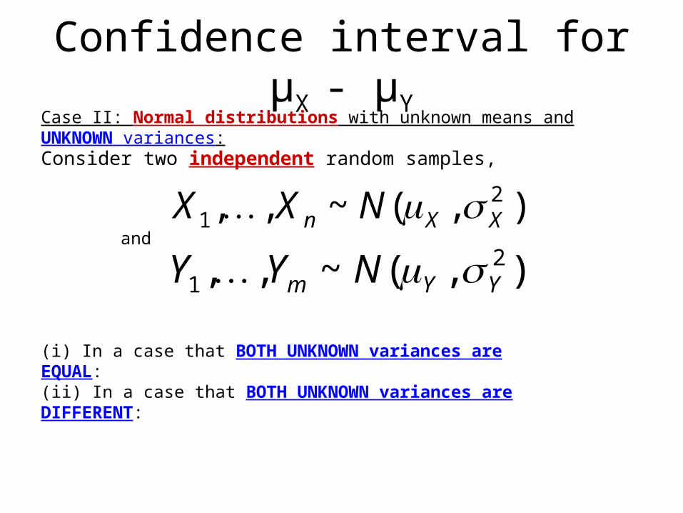
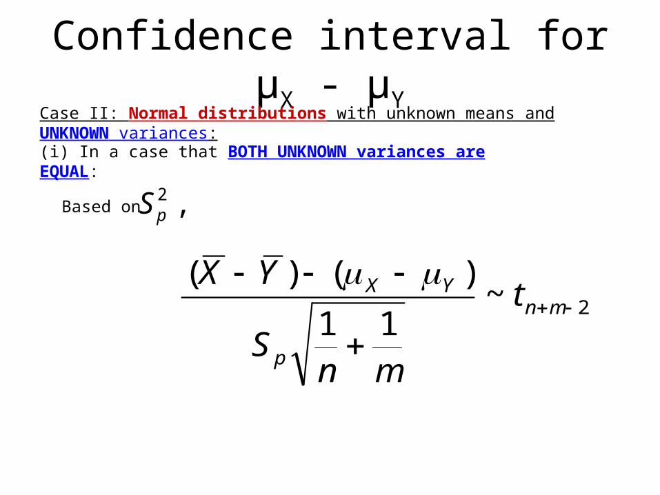
Confidence interval for µX - µY
Case II: Normal distributions with unknown means and UNKNOWN variances:
Consider two independent random samples,
),(~,, 21 XXn NXX
),(~,, 21 YYm NYY
and
(i) In a case that BOTH UNKNOWN variances are EQUAL:
(ii) In a case that BOTH UNKNOWN variances are DIFFERENT:
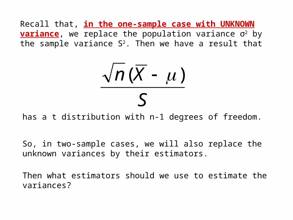
Recall that, in the one-sample case with UNKNOWN variance, we replace the population variance σ2 by the sample variance S2. Then we have a result that
S
Xn )(
has a t distribution with n-1 degrees of freedom.
So, in two-sample cases, we will also replace the unknown variances by their estimators.
Then what estimators should we use to estimate the variances?
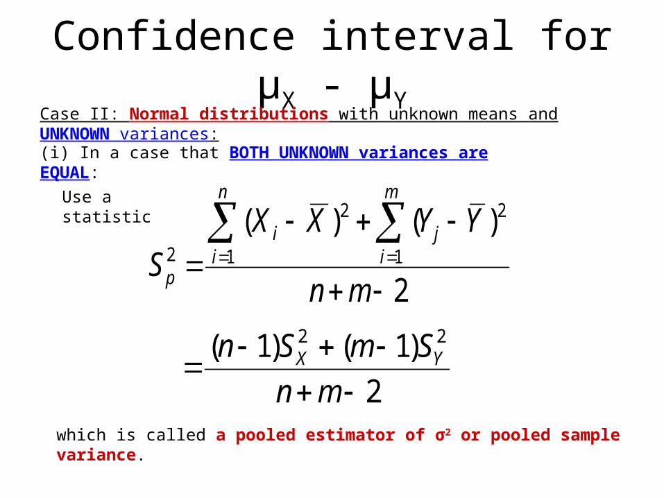
(i) In a case that BOTH UNKNOWN variances are EQUAL:
Confidence interval for µX - µY
Case II: Normal distributions with unknown means and UNKNOWN variances:
Use a statistic
which is called a pooled estimator of σ2 or pooled sample variance.
2
)()(1 1
22
2
mn
YYXXS
n
i
m
iji
p
2
)1()1( 22
mn
SmSn YX
(i) In a case that BOTH UNKNOWN variances are EQUAL:
Confidence interval for µX - µY
Case II: Normal distributions with unknown means and UNKNOWN variances:
Based on ,2pS
2~11
)()(
mn
p
YX t
mnS
YX
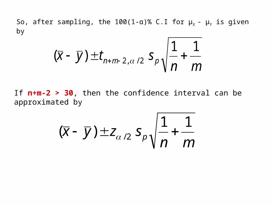
If n+m-2 > 30, then the confidence interval can be approximated by
mnszyx p
11)( 2/
So, after sampling, the 100(1-α)% C.I for μX - μY is given by
mnstyx pmn
11)( 2/,2
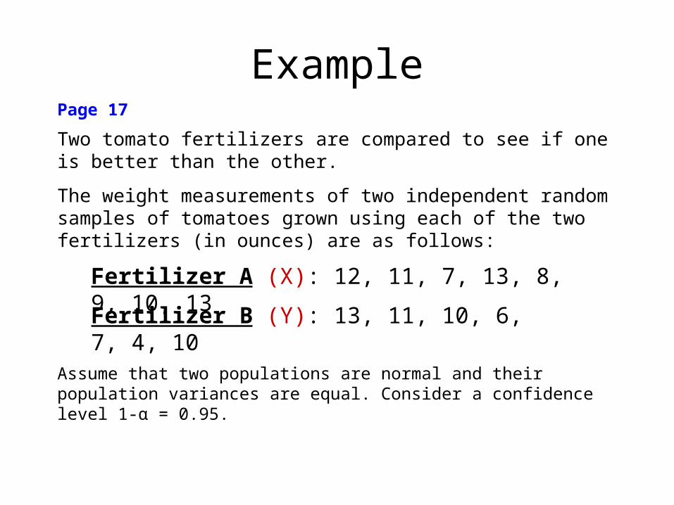
ExamplePage 17
Two tomato fertilizers are compared to see if one is better than the other.
The weight measurements of two independent random samples of tomatoes grown using each of the two fertilizers (in ounces) are as follows:
Fertilizer A (X): 12, 11, 7, 13, 8, 9, 10, 13
Fertilizer B (Y): 13, 11, 10, 6, 7, 4, 10
Assume that two populations are normal and their population variances are equal. Consider a confidence level 1-α = 0.95.
Fertilizer A (X): 12, 11, 7, 13, 8, 9, 10, 13
Fertilizer B (Y): 13, 11, 10, 6, 7, 4, 10
Assume that two populations are normal and their population variances are equal. Consider a confidence level 1-α = 0.95.
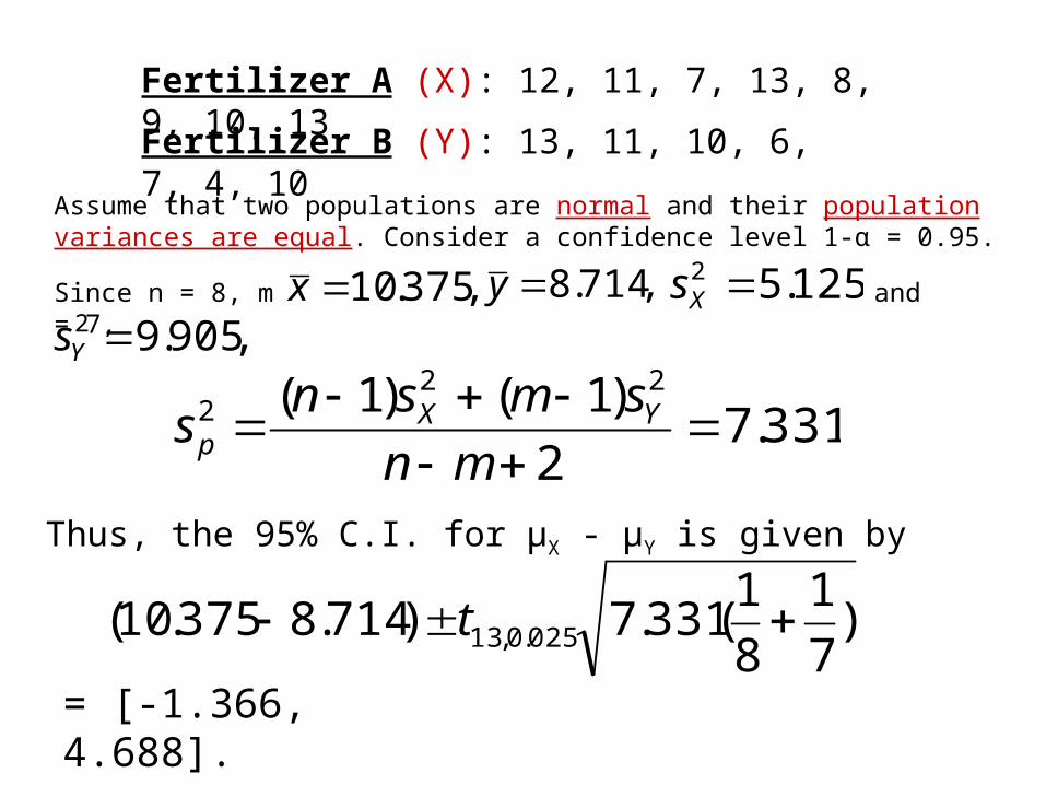
Since n = 8, m = 7,
,375.10x ,714.8y 125.52 Xs,905.92 Ys
and
331.72
)1()1( 222
mn
smsns YXp
Thus, the 95% C.I. for µX - µY is given by
)7
1
8
1(331.7)714.8375.10( 025.0,13 t
= [-1.366, 4.688].
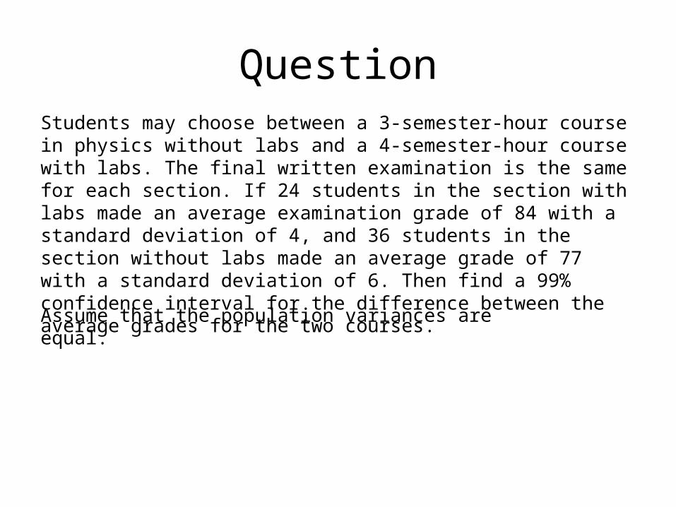
QuestionStudents may choose between a 3-semester-hour course in physics without labs and a 4-semester-hour course with labs. The final written examination is the same for each section. If 24 students in the section with labs made an average examination grade of 84 with a standard deviation of 4, and 36 students in the section without labs made an average grade of 77 with a standard deviation of 6. Then find a 99% confidence interval for the difference between the average grades for the two courses.
Assume that the population variances are equal.
Confidence interval for µX- µY
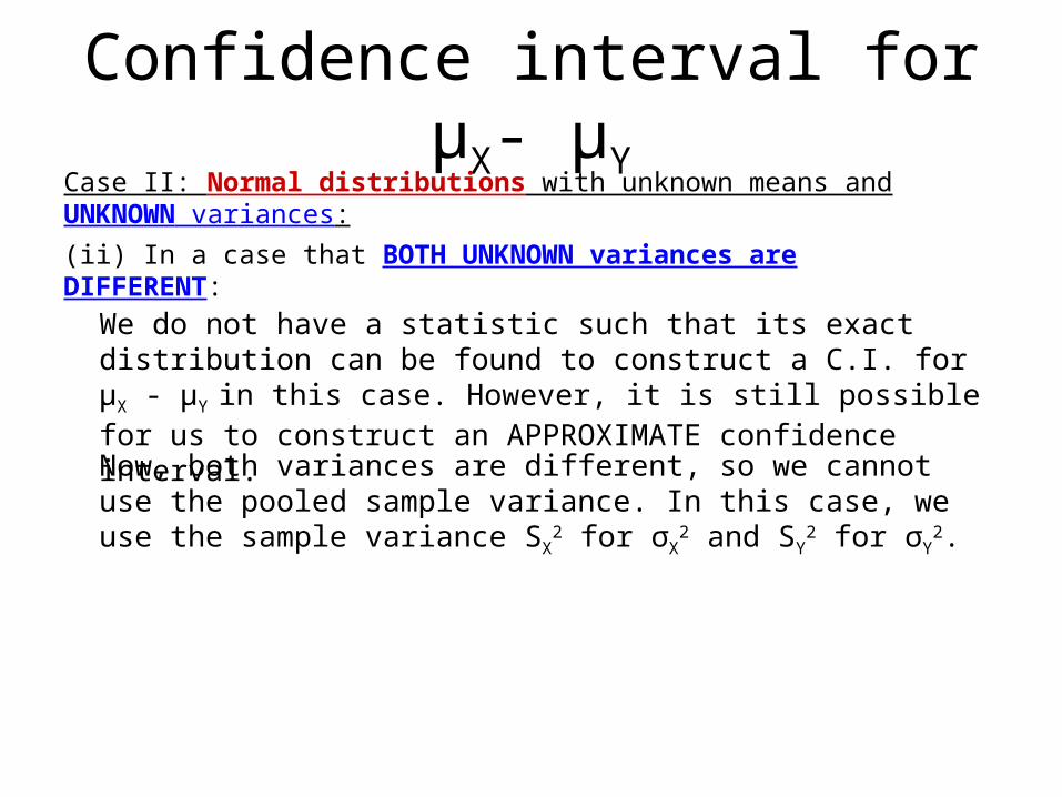
Case II: Normal distributions with unknown means and UNKNOWN variances:
(ii) In a case that BOTH UNKNOWN variances are DIFFERENT:
We do not have a statistic such that its exact distribution can be found to construct a C.I. for µX - µY in this case. However, it is still possible for us to construct an APPROXIMATE confidence interval.
Now, both variances are different, so we cannot use the pooled sample variance. In this case, we use the sample variance SX
2 for σX
2 and SY2 for σY
2.
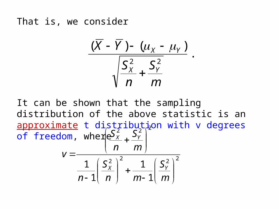
That is, we consider
.)()(
22
mS
nS
YX
YX
YX
It can be shown that the sampling distribution of the above statistic is an approximate t distribution with v degrees of freedom, where
2222
222
11
11
mS
mnS
n
mS
nS
vYX
YX
2222
222
11
11
mS
mnS
n
mS
nS
vYX
YX
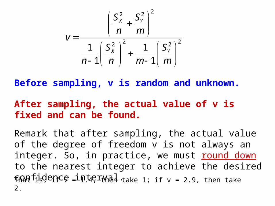
Before sampling, v is random and unknown.
After sampling, the actual value of v is fixed and can be found.
Remark that after sampling, the actual value of the degree of freedom v is not always an integer. So, in practice, we must round down to the nearest integer to achieve the desired confidence interval.
That is, if v = 1.4, then take 1; if v = 2.9, then take 2.
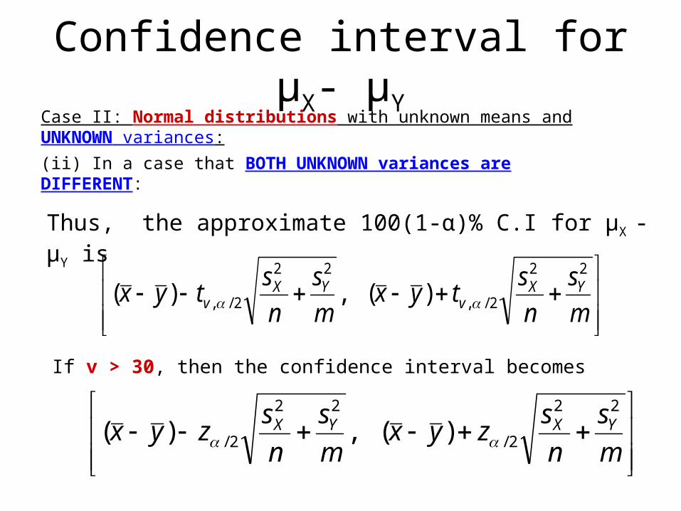
Confidence interval for µX- µY
Case II: Normal distributions with unknown means and UNKNOWN variances:
(ii) In a case that BOTH UNKNOWN variances are DIFFERENT:
m
s
n
styx
m
s
n
styx YX
vYX
v
22
2/,
22
2/, )(,)(
Thus, the approximate 100(1-α)% C.I for μX - μY is
If v > 30, then the confidence interval becomes
m
s
n
szyx
m
s
n
szyx YXYX
22
2/
22
2/ )(,)(
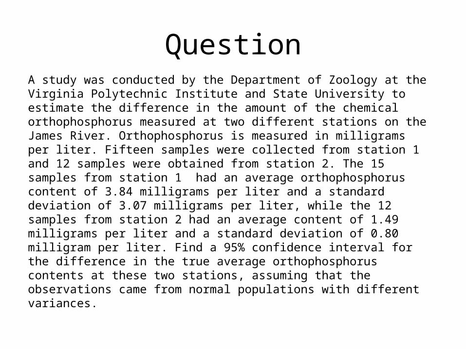
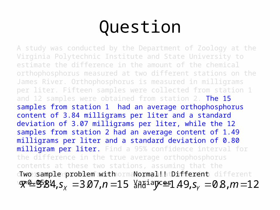
QuestionA study was conducted by the Department of Zoology at the Virginia Polytechnic Institute and State University to estimate the difference in the amount of the chemical orthophosphorus measured at two different stations on the James River. Orthophosphorus is measured in milligrams per liter. Fifteen samples were collected from station 1 and 12 samples were obtained from station 2. The 15 samples from station 1 had an average orthophosphorus content of 3.84 milligrams per liter and a standard deviation of 3.07 milligrams per liter, while the 12 samples from station 2 had an average content of 1.49 milligrams per liter and a standard deviation of 0.80 milligram per liter. Find a 95% confidence interval for the difference in the true average orthophosphorus contents at these two stations, assuming that the observations came from normal populations with different variances.
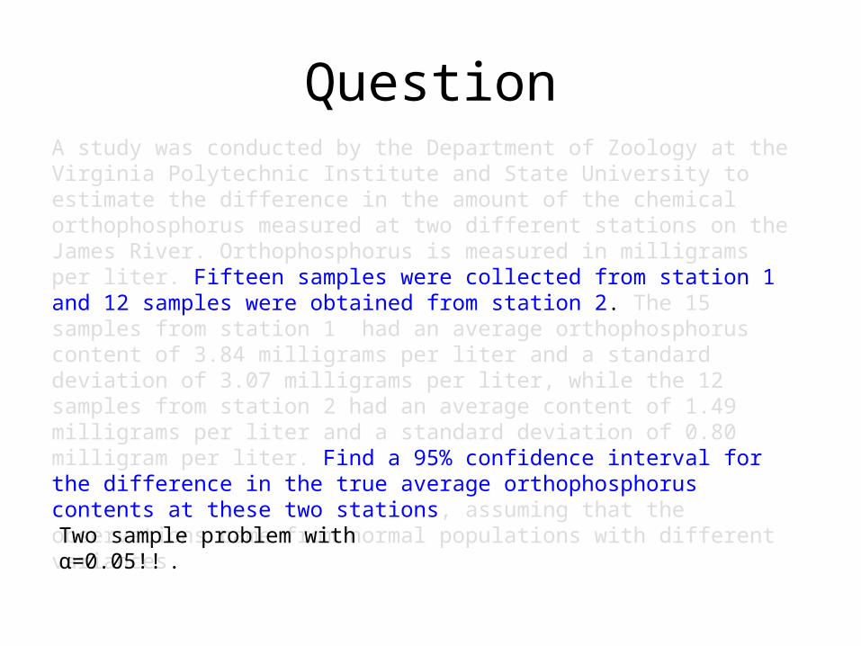
QuestionA study was conducted by the Department of Zoology at the Virginia Polytechnic Institute and State University to estimate the difference in the amount of the chemical orthophosphorus measured at two different stations on the James River. Orthophosphorus is measured in milligrams per liter. Fifteen samples were collected from station 1 and 12 samples were obtained from station 2. The 15 samples from station 1 had an average orthophosphorus content of 3.84 milligrams per liter and a standard deviation of 3.07 milligrams per liter, while the 12 samples from station 2 had an average content of 1.49 milligrams per liter and a standard deviation of 0.80 milligram per liter. Find a 95% confidence interval for the difference in the true average orthophosphorus contents at these two stations, assuming that the observations came from normal populations with different variances.
Two sample problem with α=0.05!!
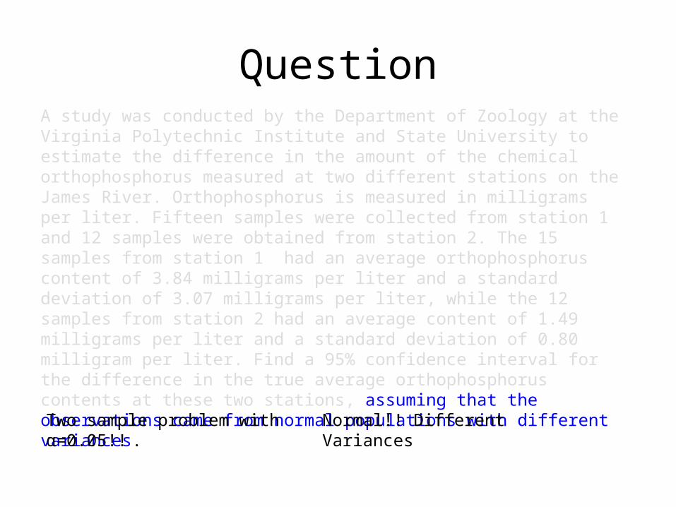
QuestionA study was conducted by the Department of Zoology at the Virginia Polytechnic Institute and State University to estimate the difference in the amount of the chemical orthophosphorus measured at two different stations on the James River. Orthophosphorus is measured in milligrams per liter. Fifteen samples were collected from station 1 and 12 samples were obtained from station 2. The 15 samples from station 1 had an average orthophosphorus content of 3.84 milligrams per liter and a standard deviation of 3.07 milligrams per liter, while the 12 samples from station 2 had an average content of 1.49 milligrams per liter and a standard deviation of 0.80 milligram per liter. Find a 95% confidence interval for the difference in the true average orthophosphorus contents at these two stations, assuming that the observations came from normal populations with different variances.
Normal!! Different VariancesTwo sample problem with α=0.05!!
15,07.3,84.3 nsx X 12,8.0,49.1 msy Yand
QuestionNormal!! Different VariancesTwo sample problem with α=0.05!!
15,07.3,84.3 nsx X 12,8.0,49.1 msy Yand
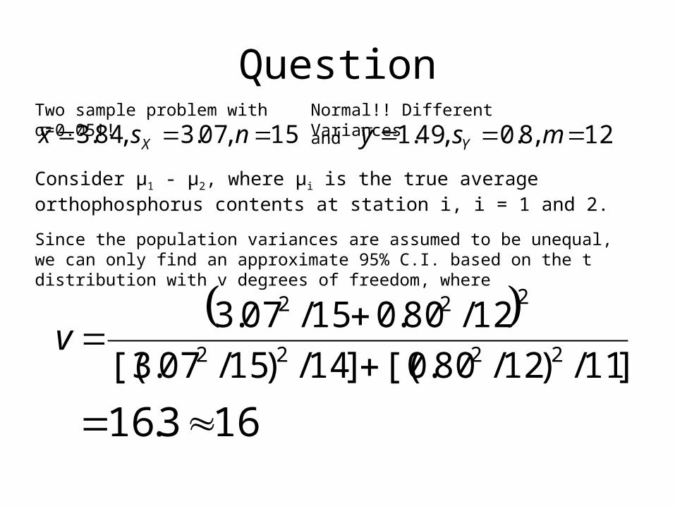
Consider µ1 - µ2, where µi is the true average orthophosphorus contents at station i, i = 1 and 2.
Since the population variances are assumed to be unequal, we can only find an approximate 95% C.I. based on the t distribution with v degrees of freedom, where
]11/)12/80.0[(]14/)15/07.3[(
12/80.015/07.32222
222
v
163.16
QuestionNormal!! Different VariancesTwo sample problem with α=0.05!!
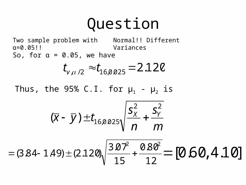
So, for α = 0.05, we have
120.2025.0,162/, ttv
m
s
n
styx YX
22
025.0,16)(
Thus, the 95% C.I. for µ1 - µ2 is
].10.4,60.0[12
80.0
15
07.3)120.2()49.184.3(
22
Question
m
s
n
styx YX
22
025.0,16)(
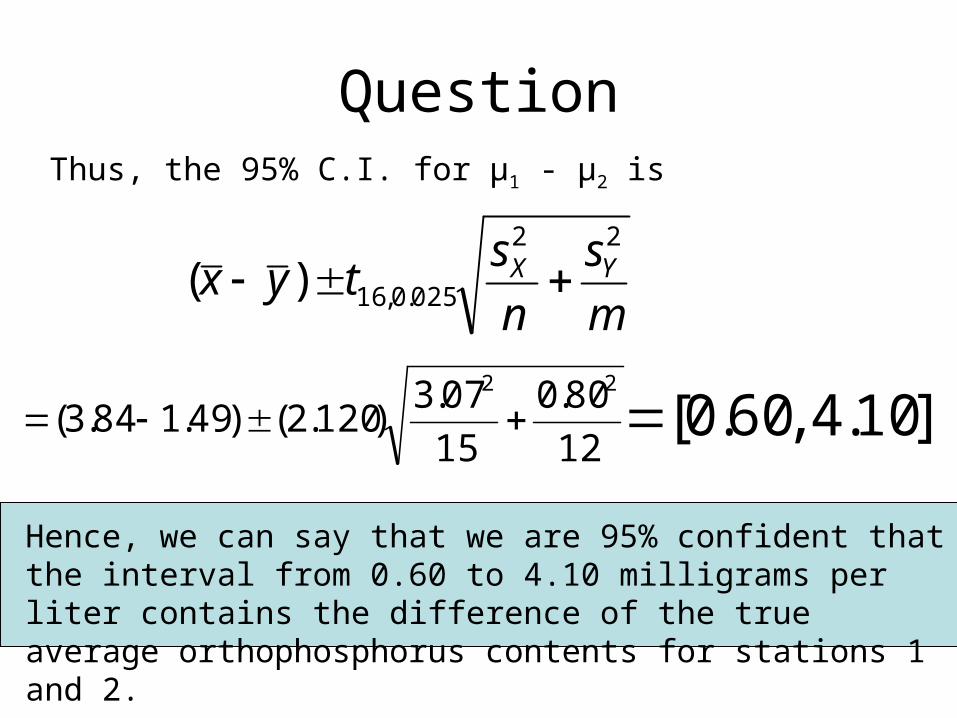
Thus, the 95% C.I. for µ1 - µ2 is
].10.4,60.0[12
80.0
15
07.3)120.2()49.184.3(
22
Hence, we can say that we are 95% confident that the interval from 0.60 to 4.10 milligrams per liter contains the difference of the true average orthophosphorus contents for stations 1 and 2.
One- (or Two-) sample(s)
Confidence Interval for µX (or µX - µY) with NON-NORMAL population(s)
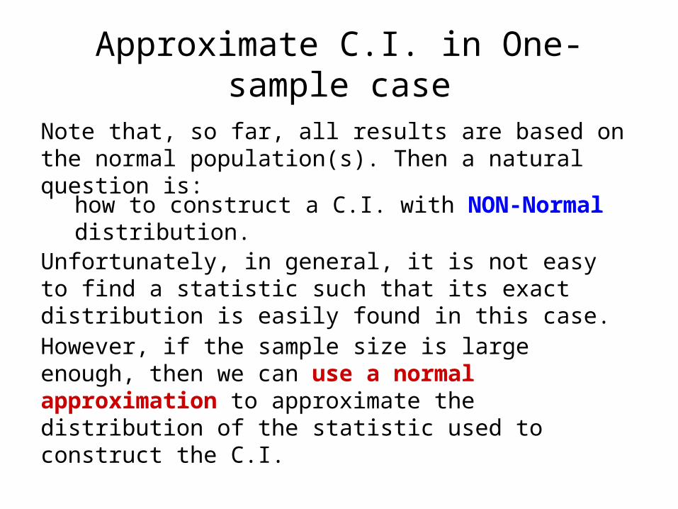
Approximate C.I. in One-sample case
Note that, so far, all results are based on the normal population(s). Then a natural question is:
how to construct a C.I. with NON-Normal distribution.
Unfortunately, in general, it is not easy to find a statistic such that its exact distribution is easily found in this case.
However, if the sample size is large enough, then we can use a normal approximation to approximate the distribution of the statistic used to construct the C.I.
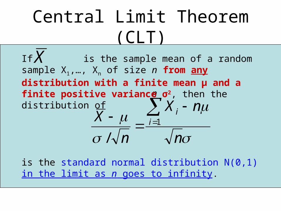
Central Limit Theorem (CLT)
n
nX
n
X
n
ii
1
/
If is the sample mean of a random sample X1,…, Xn of size n from any distribution with a finite mean µ and a finite positive variance σ2, then the distribution of
X
is the standard normal distribution N(0,1) in the limit as n goes to infinity.
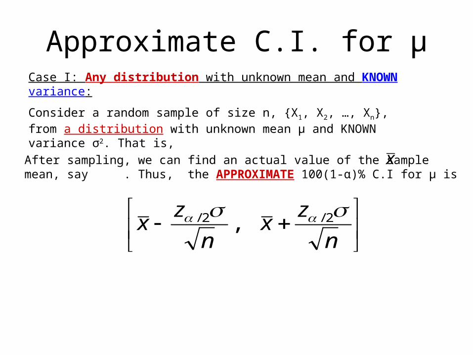
Approximate C.I. for µCase I: Any distribution with unknown mean and KNOWN variance:
Consider a random sample of size n, {X1, X2, …, Xn}, from a distribution with unknown mean µ and KNOWN variance σ2. That is,
n
zx
n
zx
2/2/ ,
xAfter sampling, we can find an actual value of the sample mean, say . Thus, the APPROXIMATE 100(1-α)% C.I for μ is
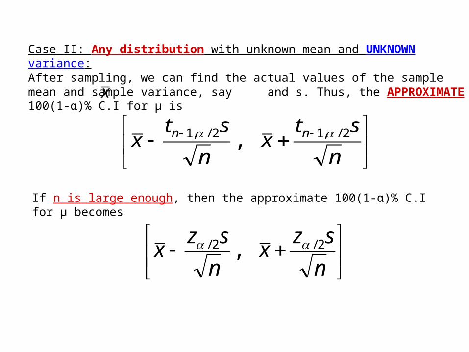
Case II: Any distribution with unknown mean and UNKNOWN variance:
n
stx
n
stx nn 2/,12/,1 ,
xAfter sampling, we can find the actual values of the sample mean and sample variance, say and s. Thus, the APPROXIMATE 100(1-α)% C.I for μ is
If n is large enough, then the approximate 100(1-α)% C.I for μ becomes
n
szx
n
szx 2/2/ ,
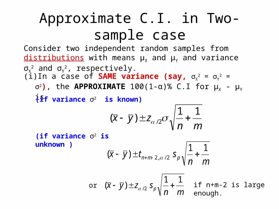
Approximate C.I. in Two-sample case
Consider two independent random samples from distributions with means µX and µY and variance σX
2 and σY2, respectively.
(i) In a case of SAME variance (say, σX2 = σY
2 = σ2), the APPROXIMATE 100(1-α)% C.I for µX - µY is
(if variance σ2 is known)
mnzyx
11)( 2/
(if variance σ2 is unknown )
mnstyx pmn
11)( 2/,2
mnszyx p
11)( 2/ or if n+m-2 is large enough.
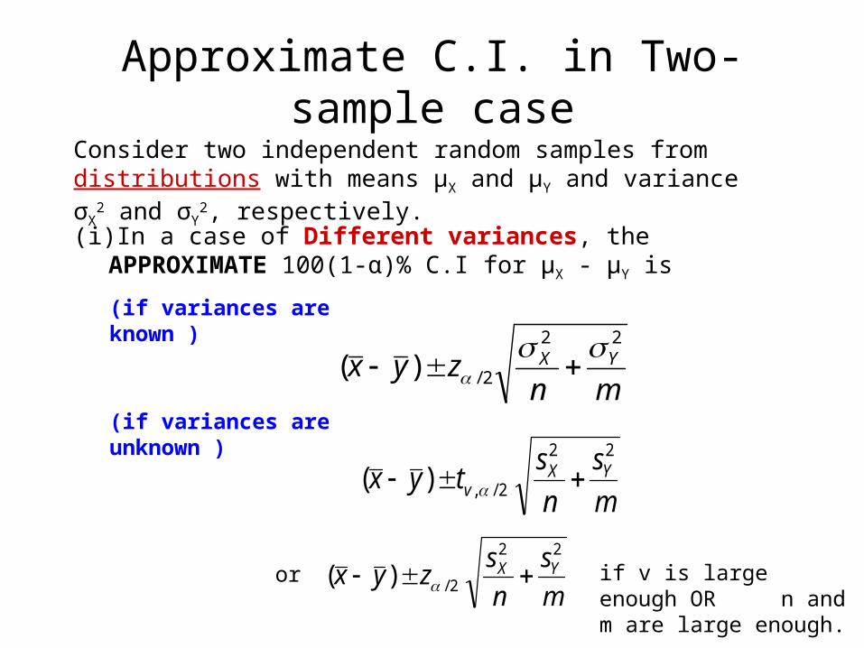
Approximate C.I. in Two-sample case
Consider two independent random samples from distributions with means µX and µY and variance σX
2 and σY2, respectively.
(i) In a case of Different variances, the APPROXIMATE 100(1-α)% C.I for µX - µY is
(if variances are known )
mnzyx YX
22
2/)(
(if variances are unknown )
m
s
n
styx YXv
22
2/,)(
m
s
n
szyx YX
22
2/)( or if v is large enough OR n and m are large enough.
Confidence Interval for σ2
with NORMAL population
Confidence interval for σ2
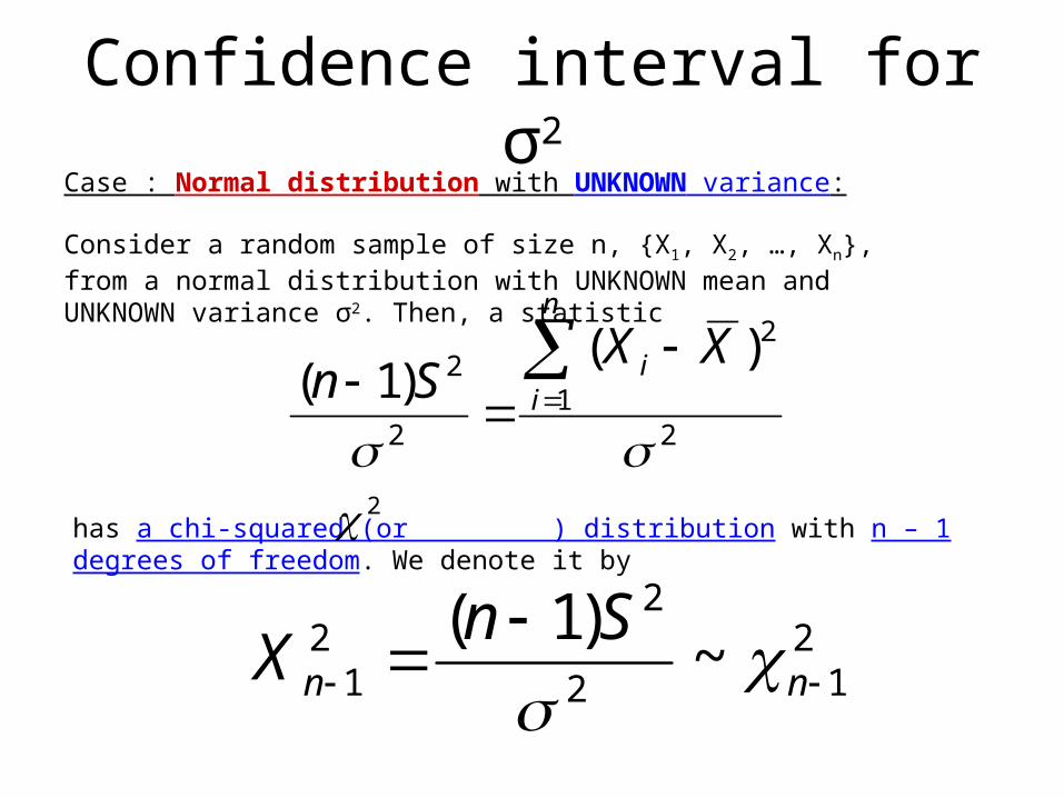
Case : Normal distribution with UNKNOWN variance:
Consider a random sample of size n, {X1, X2, …, Xn}, from a normal distribution with UNKNOWN mean and UNKNOWN variance σ2. Then, a statistic
21
2
2
2 )()1(
n
ii XX
Sn
has a chi-squared (or ) distribution with n – 1 degrees of freedom. We denote it by
2
212
221 ~
)1(
nn
SnX
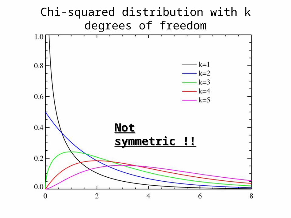
Chi-squared distribution with k degrees of freedom
Not symmetric !!Not symmetric !!
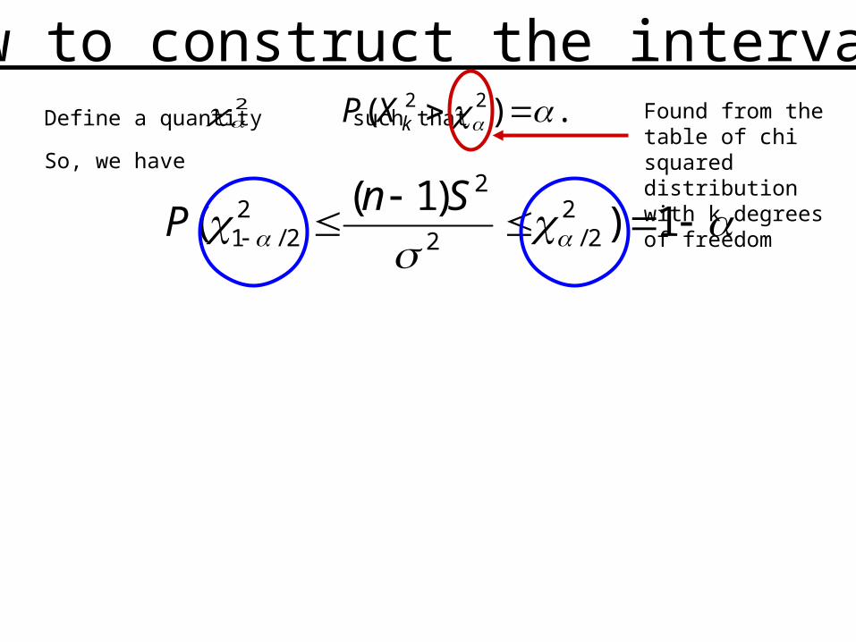
How to construct the interval?
1))1(
( 22/2
22
2/1
SnP
So, we have
2 .)( 22 kXPDefine a quantity such that Found from the table
of chi squared distribution with k degrees of freedom
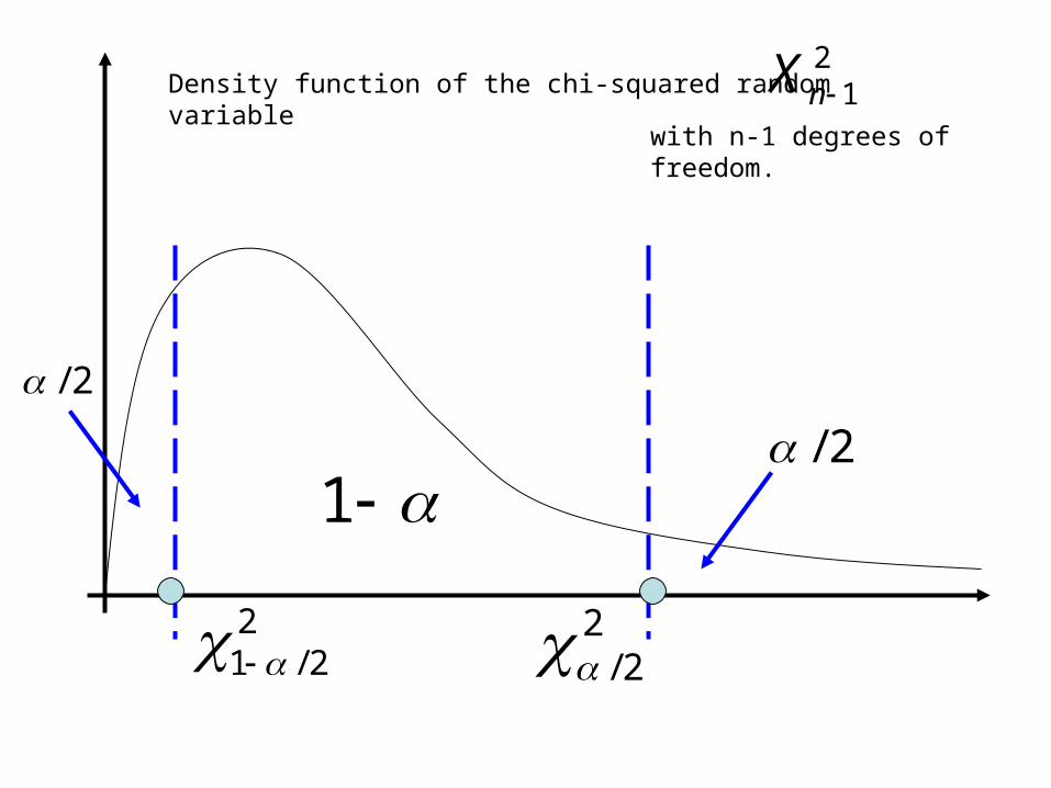
Density function of the chi-squared random variable21nX
with n-1 degrees of freedom.
2/2/
1
22/
22/1
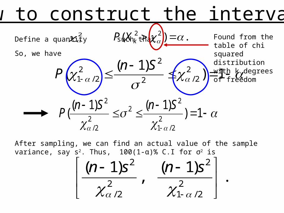
How to construct the interval?
.)1(
,)1(
22/1
2
22/
2
snsn
1))1(
( 22/2
22
2/1
SnP
So, we have
1))1()1(
(2
2/1
22
22/
2 SnSnP
2 .)( 22 kXPDefine a quantity such that
After sampling, we can find an actual value of the sample variance, say s2. Thus, 100(1-α)% C.I for σ2 is
Found from the table of chi squared distribution with k degrees of freedom
How to use the table of chi-squared distribution
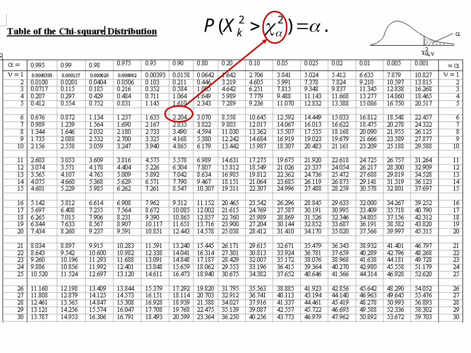
.)( 22 kXP
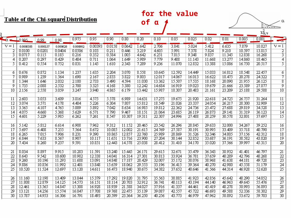
for the value of α
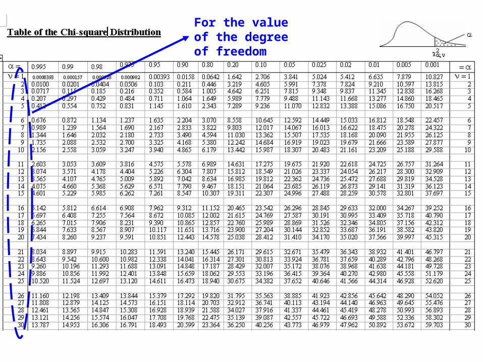
For the value of the degree of freedom
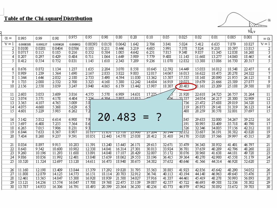
20.483 = ?
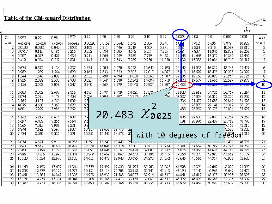
20.483 = ?2025.0
With 10 degrees of freedom
QuestionsPage 21
For a chi-squared distribution with v degrees of freedom,
a) If v = 5, then
2005.0
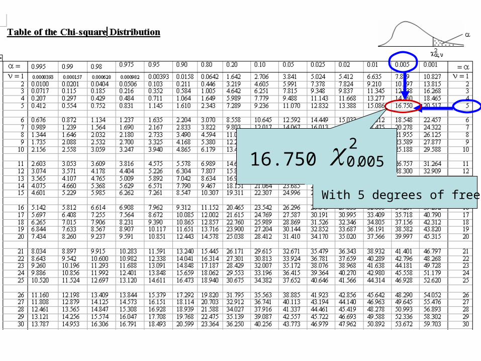
16.750 = 2005.0
With 5 degrees of freedom
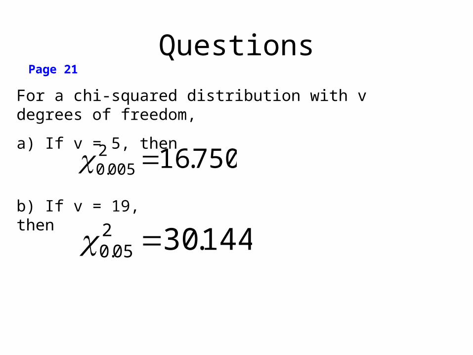
QuestionsPage 21
For a chi-squared distribution with v degrees of freedom,
a) If v = 5, then
b) If v = 19, then
750.162005.0
144.30205.0
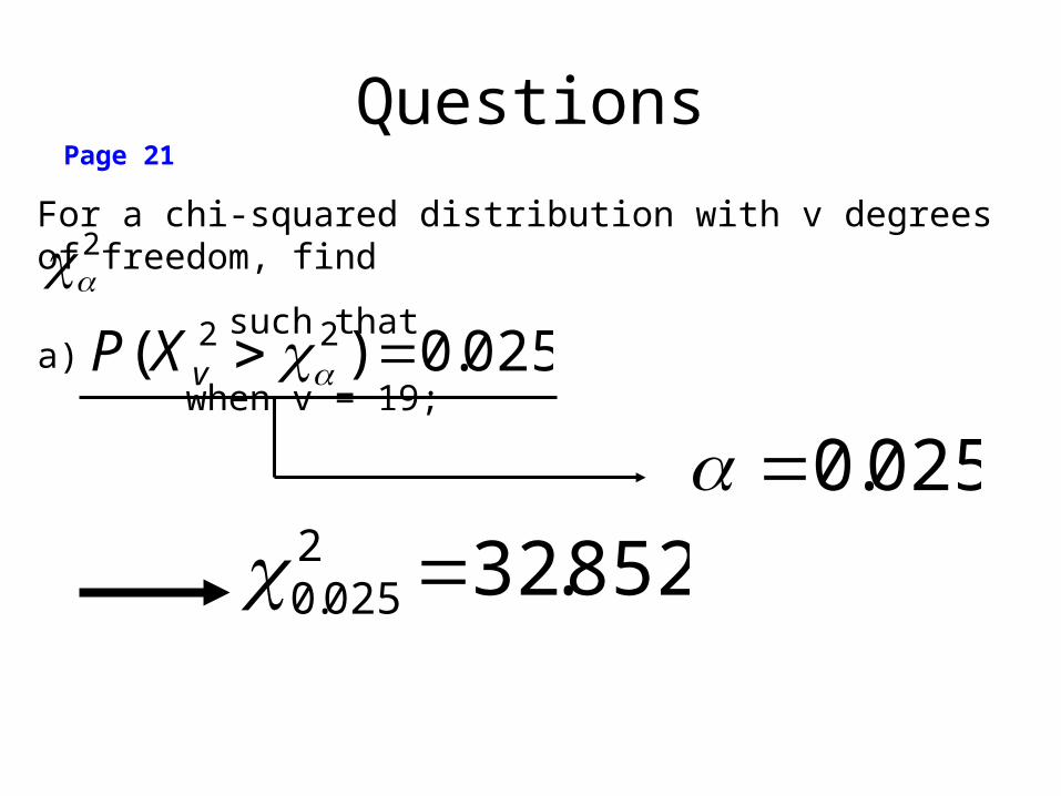
QuestionsPage 21
For a chi-squared distribution with v degrees of freedom, find
such that2
025.0)( 22 vXPa) when v = 19;
025.0852.322
025.0
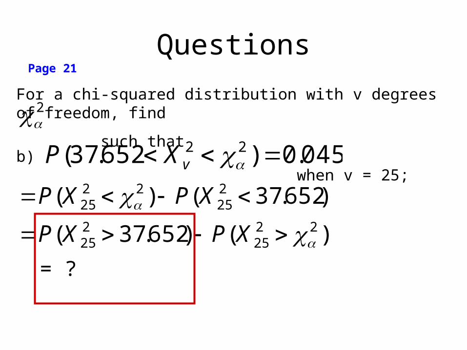
QuestionsPage 21
For a chi-squared distribution with v degrees of freedom, find
such that2
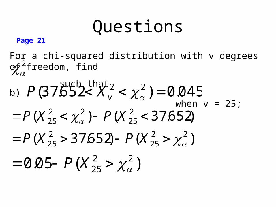
045.0)652.37( 22 vXPb) when v = 25;
)()652.37(
)652.37()(22
25225
225
2225
XPXP
XPXP
= ?
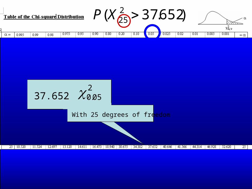
)652.37( 225 XP
37.652 = 205.0
With 25 degrees of freedom
QuestionsPage 21
For a chi-squared distribution with v degrees of freedom, find
such that2
045.0)652.37( 22 vXPb) when v = 25;
)()652.37(
)652.37()(22
25225
225
2225
XPXP
XPXP
)(05.0 2225 XP
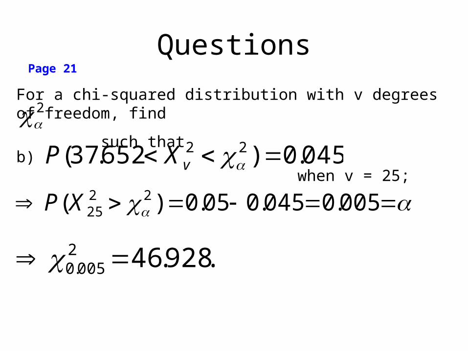
QuestionsPage 21
For a chi-squared distribution with v degrees of freedom, find
such that2
045.0)652.37( 22 vXPb) when v = 25;
005.0045.005.0)( 2225XP
.928.462005.0
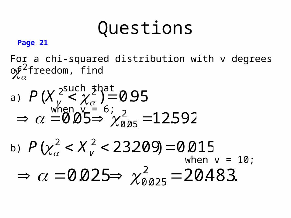
QuestionsPage 21
For a chi-squared distribution with v degrees of freedom, find
such that2
.483.20025.0 2025.0
95.0)( 22 vXPa) when v = 6;
592.1205.0 205.0
015.0)209.23( 22 vXP b) when v = 10;
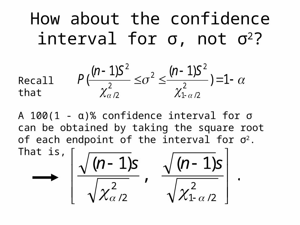
How about the confidence interval for σ, not σ2?
A 100(1 - α)% confidence interval for σ can be obtained by taking the square root of each endpoint of the interval for σ2. That is,
.)1(
,)1(
22/1
22/
snsn
1))1()1(
(2
2/1
22
22/
2 SnSnPRecall that
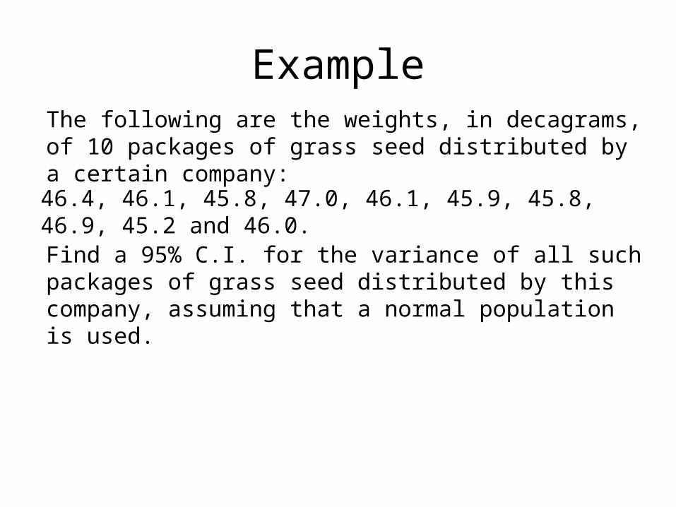
ExampleThe following are the weights, in decagrams, of 10 packages of grass seed distributed by a certain company:
46.4, 46.1, 45.8, 47.0, 46.1, 45.9, 45.8, 46.9, 45.2 and 46.0.
Find a 95% C.I. for the variance of all such packages of grass seed distributed by this company, assuming that a normal population is used.
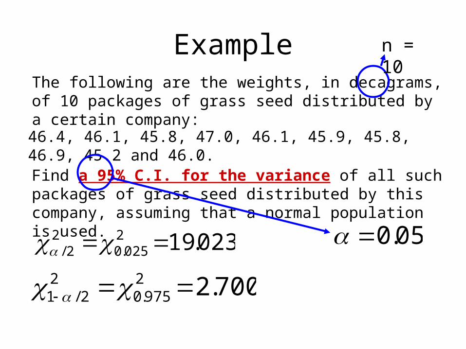
700.22975.0
22/1
05.0
n = 10
023.192025.0
22/
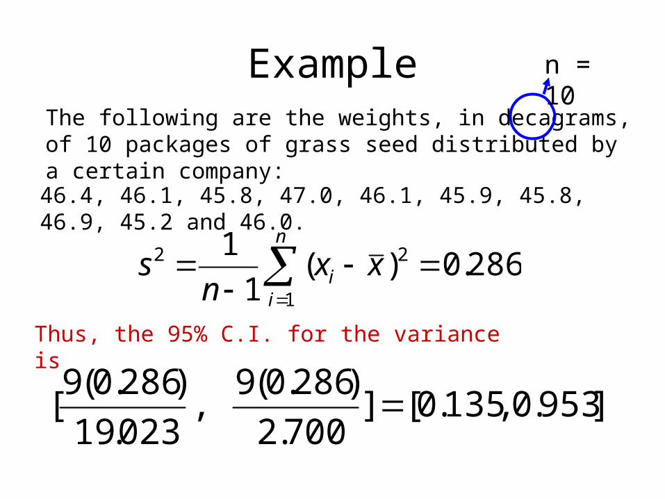
ExampleThe following are the weights, in decagrams, of 10 packages of grass seed distributed by a certain company:
46.4, 46.1, 45.8, 47.0, 46.1, 45.9, 45.8, 46.9, 45.2 and 46.0.
n
ii xx
ns
1
22 286.0)(1
1
n = 10
Thus, the 95% C.I. for the variance is
].953.0,135.0[]700.2
)286.0(9,
023.19
)286.0(9[
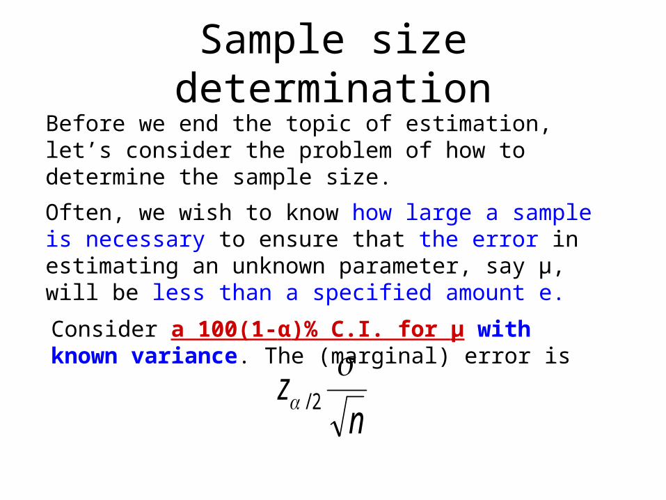
Sample size determinationBefore we end the topic of estimation, let’s consider the problem of how to determine the sample size.
Often, we wish to know how large a sample is necessary to ensure that the error in estimating an unknown parameter, say µ, will be less than a specified amount e.
Consider a 100(1-α)% C.I. for µ with known variance. The (marginal) error is
nz
2/
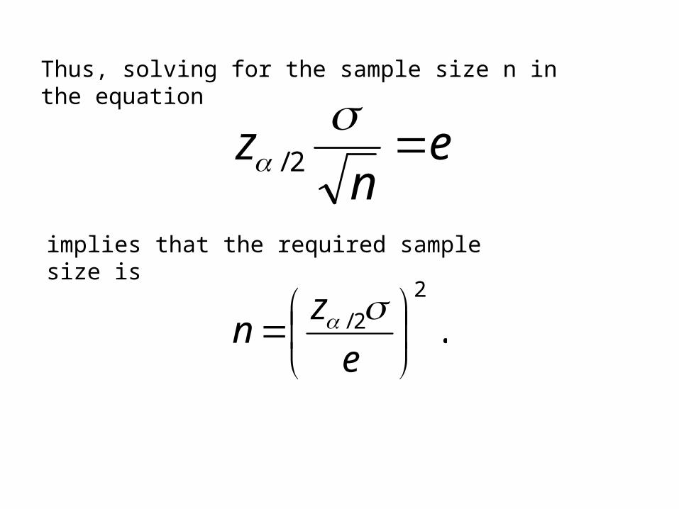
Thus, solving for the sample size n in the equation
en
z
2/
implies that the required sample size is
.2
2/
e
zn
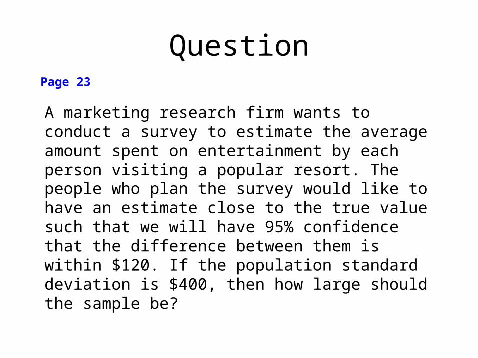
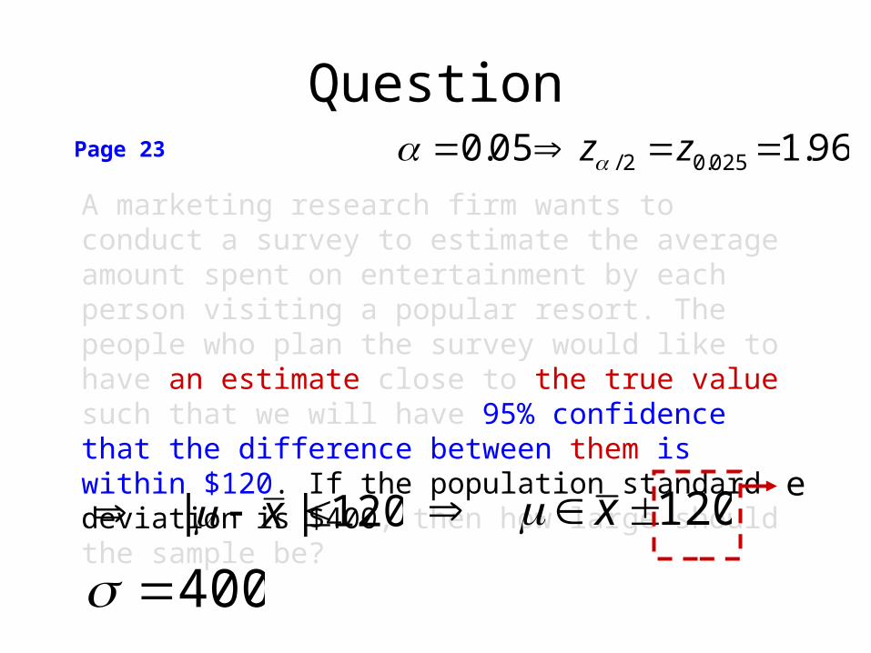
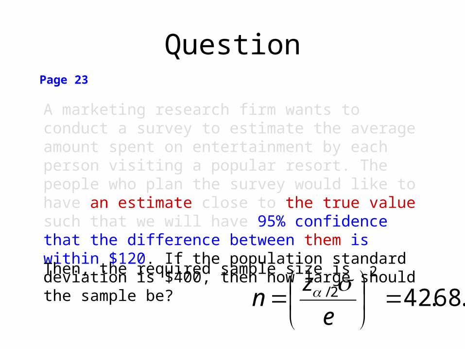
QuestionPage 23
A marketing research firm wants to conduct a survey to estimate the average amount spent on entertainment by each person visiting a popular resort. The people who plan the survey would like to have an estimate close to the true value such that we will have 95% confidence that the difference between them is within $120. If the population standard deviation is $400, then how large should the sample be?
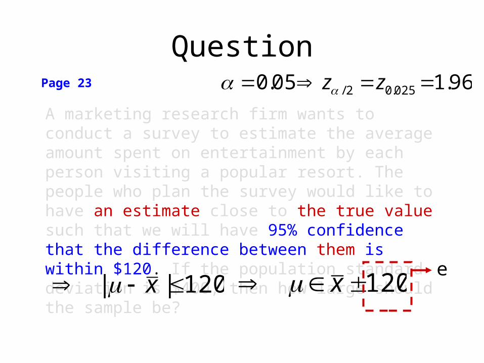
120|| x 120 x e
96.105.0 025.02/ zz
400
QuestionPage 23
A marketing research firm wants to conduct a survey to estimate the average amount spent on entertainment by each person visiting a popular resort. The people who plan the survey would like to have an estimate close to the true value such that we will have 95% confidence that the difference between them is within $120. If the population standard deviation is $400, then how large should the sample be?
Then, the required sample size is
.68.422
2/
e
zn


![Opus 144, Six Fairy Tales for Flute Solo [Opus 144]](https://img.pdfslide.us/doc/110x75/61e4550386b9437ad2408547/opus-144-six-fairy-tales-for-flute-solo-opus-144.jpg)