1

Math 140 Final Exam Fall 2016 Name: SOLUTIONS

VERSION 3 Instructor:

Days and Time of Class:

INSTRUCTIONS

• SHOW ALL WORK, including calculator commands that you use.

• Write your final answer in the ANSWER box, if one is provided.

• Please write in pencil and erase anything that you don’t want graded.

• Graphing calculators are allowed only if nothing has been stored in them. Books and notes are NOT allowed.

• Please return the formula sheet with your exam.

• Please raise your hand when finished and pack up after your exam has been collected.

• No cell phones may be turned on or in sight at any time during the exam. If your phone is visible during the exam, your papers will be collected and you will receive an F on the exam.

Problem Possible Points Points Scored

1 4

2 6

3 6

4 8

5 9

6 9

7 13

8 15

9 14

10 6

11 10

TOTAL 100

2

1. The number of long-term unemployed (those jobless for 27 weeks or more) was 1.9 million in November 2016. The long-term unemployed accounted for 24.8 percent of the all unemployed people. What was the total number of unemployed?

!.!!

= .248 x = 7.661290323 million ≈ 7.66 million

OR !,!"",!!!

! = .248 x ≈ 7,661,290

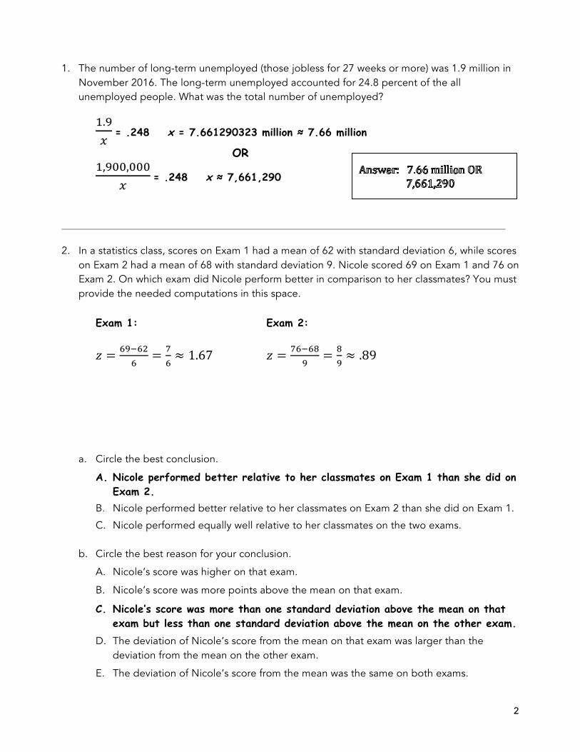
2. In a statistics class, scores on Exam 1 had a mean of 62 with standard deviation 6, while scores on Exam 2 had a mean of 68 with standard deviation 9. Nicole scored 69 on Exam 1 and 76 on Exam 2. On which exam did Nicole perform better in comparison to her classmates? You must provide the needed computations in this space.

Exam 1: Exam 2:

𝑧 = !"!!"!

= !!≈ 1.67 𝑧 = !"!!"

!= !

!≈ .89

a. Circle the best conclusion.

A. Nicole performed better relative to her classmates on Exam 1 than she did on Exam 2.

B. Nicole performed better relative to her classmates on Exam 2 than she did on Exam 1.

C. Nicole performed equally well relative to her classmates on the two exams.

b. Circle the best reason for your conclusion.

A. Nicole’s score was higher on that exam.

B. Nicole’s score was more points above the mean on that exam.

C. Nicole’s score was more than one standard deviation above the mean on that exam but less than one standard deviation above the mean on the other exam.

D. The deviation of Nicole’s score from the mean on that exam was larger than the deviation from the mean on the other exam.

E. The deviation of Nicole’s score from the mean was the same on both exams.

3

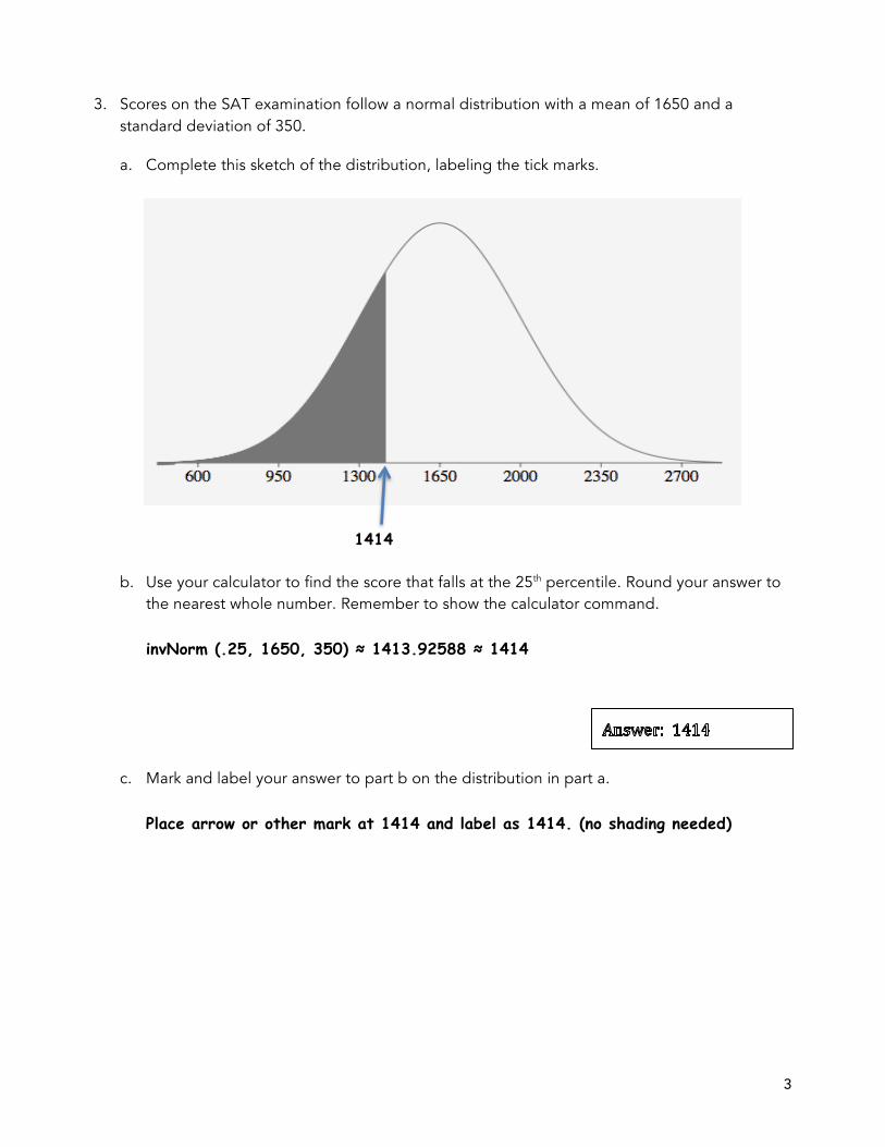
3. Scores on the SAT examination follow a normal distribution with a mean of 1650 and a standard deviation of 350.

a. Complete this sketch of the distribution, labeling the tick marks.

1414

b. Use your calculator to find the score that falls at the 25th percentile. Round your answer to the nearest whole number. Remember to show the calculator command.

invNorm (.25, 1650, 350) ≈ 1413.92588 ≈ 1414 c. Mark and label your answer to part b on the distribution in part a.

Place arrow or other mark at 1414 and label as 1414. (no shading needed)

4

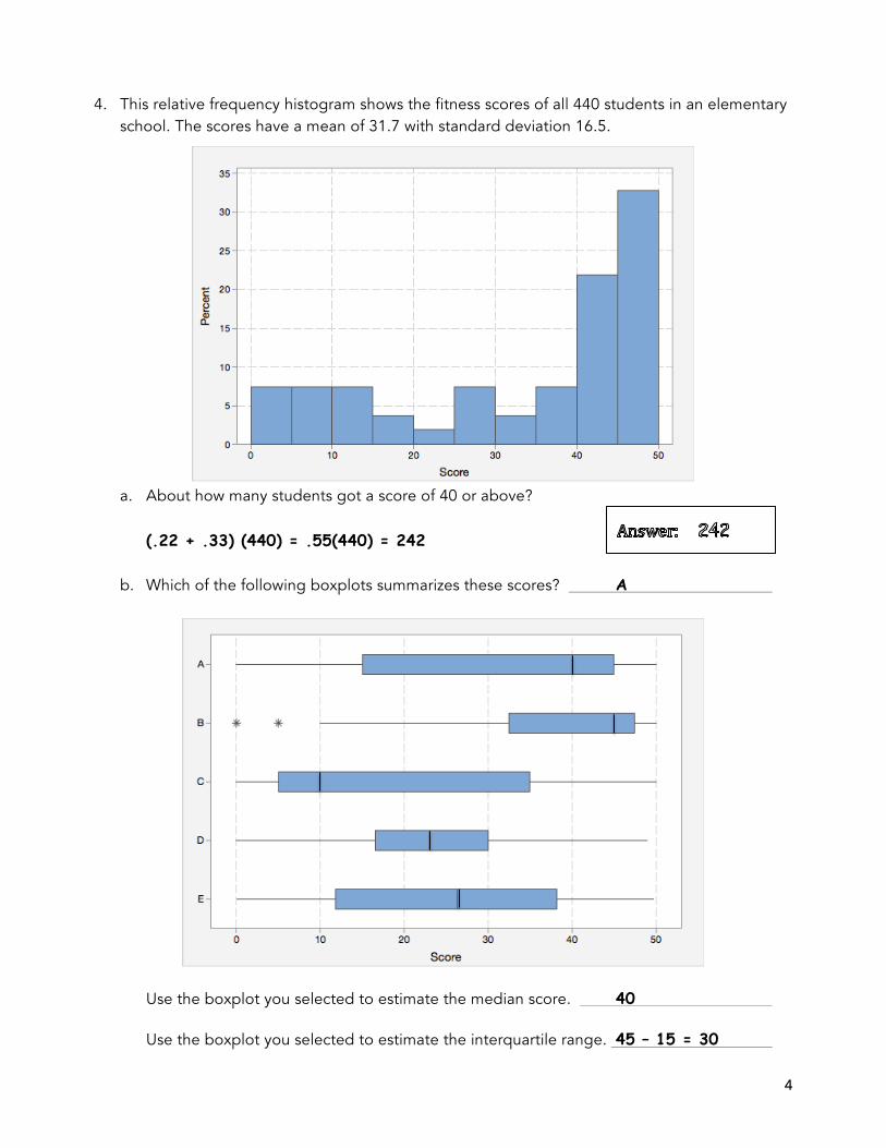
4. This relative frequency histogram shows the fitness scores of all 440 students in an elementary school. The scores have a mean of 31.7 with standard deviation 16.5.

a. About how many students got a score of 40 or above? (.22 + .33) (440) = .55(440) = 242 b. Which of the following boxplots summarizes these scores? A

Use the boxplot you selected to estimate the median score. 40

Use the boxplot you selected to estimate the interquartile range. 45 – 15 = 30

5

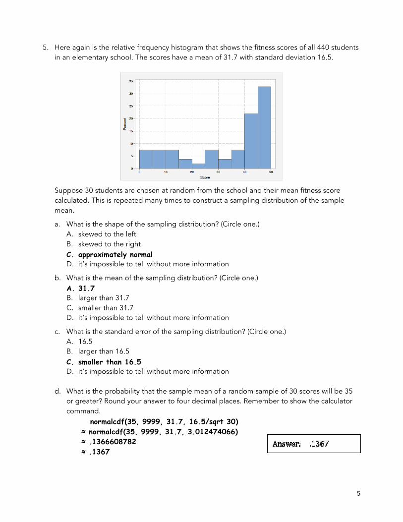
5. Here again is the relative frequency histogram that shows the fitness scores of all 440 students in an elementary school. The scores have a mean of 31.7 with standard deviation 16.5.

Suppose 30 students are chosen at random from the school and their mean fitness score calculated. This is repeated many times to construct a sampling distribution of the sample mean.

a. What is the shape of the sampling distribution? (Circle one.) A. skewed to the left B. skewed to the right C. approximately normal D. it’s impossible to tell without more information

b. What is the mean of the sampling distribution? (Circle one.) A. 31.7 B. larger than 31.7 C. smaller than 31.7 D. it’s impossible to tell without more information

c. What is the standard error of the sampling distribution? (Circle one.) A. 16.5 B. larger than 16.5 C. smaller than 16.5 D. it’s impossible to tell without more information

d. What is the probability that the sample mean of a random sample of 30 scores will be 35

or greater? Round your answer to four decimal places. Remember to show the calculator command.

normalcdf(35, 9999, 31.7, 16.5/sqrt 30) ≈ normalcdf(35, 9999, 31.7, 3.012474066) ≈ .1366608782 ≈ .1367

6

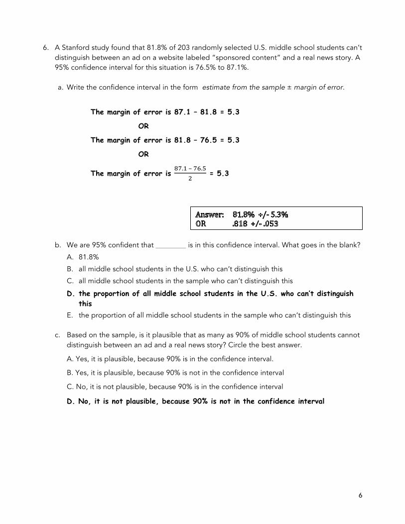
6. A Stanford study found that 81.8% of 203 randomly selected U.S. middle school students can’t distinguish between an ad on a website labeled “sponsored content” and a real news story. A 95% confidence interval for this situation is 76.5% to 87.1%.

a. Write the confidence interval in the form estimate from the sample ± margin of error.

The margin of error is 87.1 – 81.8 = 5.3

OR

The margin of error is 81.8 – 76.5 = 5.3

OR

The margin of error is !".! – !".!

! = 5.3

b. We are 95% confident that is in this confidence interval. What goes in the blank?

A. 81.8%

B. all middle school students in the U.S. who can’t distinguish this

C. all middle school students in the sample who can’t distinguish this

D. the proportion of all middle school students in the U.S. who can’t distinguish this

E. the proportion of all middle school students in the sample who can’t distinguish this

c. Based on the sample, is it plausible that as many as 90% of middle school students cannot distinguish between an ad and a real news story? Circle the best answer.

A. Yes, it is plausible, because 90% is in the confidence interval.

B. Yes, it is plausible, because 90% is not in the confidence interval

C. No, it is not plausible, because 90% is in the confidence interval

D. No, it is not plausible, because 90% is not in the confidence interval

.

7

7. In a recent survey of Americans by Pew Research, 151 (43%) out of 351 high-income individuals (defined as those earning over $75,000 a year) said that the growing number of immigrant workers in this county helps American workers. By contrast, 495 (38%) out of 1302 middle-income individuals (those earning between $30,000 and $75,000 a year) said that immigration helps American workers. Do a hypothesis test to determine if among all Americans there is a statistically significant difference in the proportions of high-income and middle-income Americans who would say that immigration helps American workers.

a. Write the hypotheses for this test. Let p1 represent the proportion of high-income Americans who would say that immigration helps Americans, and let p2 represent the proportion of middle-income Americans who would say this.

H0: p1 = p2 Ha: p1 ≠ p2

b. Compute the difference in the sample proportions: 𝑝! − 𝑝! =.43 – .38 = .05 .

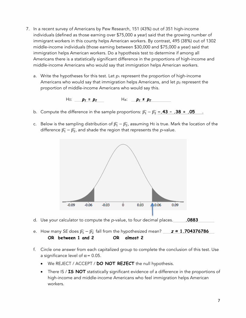
c. Below is the sampling distribution of 𝑝! − 𝑝!, assuming H0 is true. Mark the location of the difference 𝑝! − 𝑝!, and shade the region that represents the p-value.

d. Use your calculator to compute the p-value, to four decimal places. .0883

e. How many SE does 𝑝! − 𝑝! fall from the hypothesized mean? z ≈ 1.704376786 OR between 1 and 2 OR almost 2

f. Circle one answer from each capitalized group to complete the conclusion of this test. Use a significance level of α = 0.05.

• We REJECT / ACCEPT / DO NOT REJECT the null hypothesis.

• There IS / IS NOT statistically significant evidence of a difference in the proportions of high-income and middle-income Americans who feel immigration helps American workers.

8

8. The name Brittany was very popular a few years ago. In the U.S., the mean age of women with that name is 23.5 years. You think that Emilys are even younger, on average. You get a random sample of 15 Emilys and their average age is 20.2 years with a standard deviation of 6.2 years. Is this statistically significant evidence that you are correct?

a. Which of the numbers above is the sample mean? 20.2 b. The null hypothesis is H0: µ = 23.5. Write the alternative hypothesis Ha: µ < 23.5

What does µ represent? Circle the best answer.

A. 20.2

B. 23.5

C. the sample mean

D. the mean age of all Emilys in the U.S. E. the mean age of all Brittanys in the U.S.

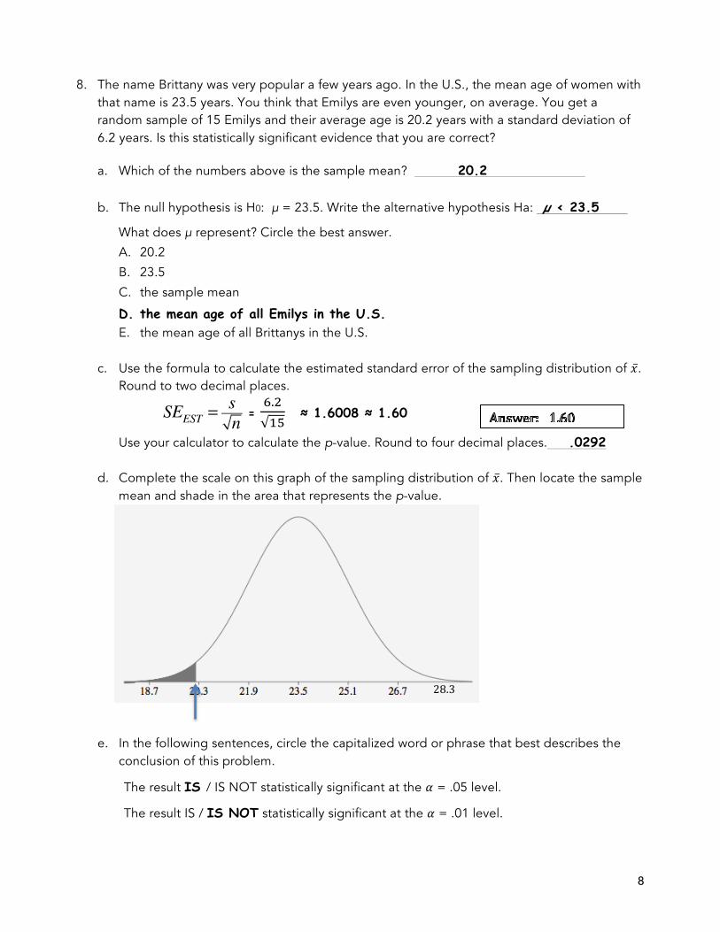
c. Use the formula to calculate the estimated standard error of the sampling distribution of 𝑥.

Round to two decimal places.

SEEST =sn =

!.!!"

≈ 1.6008 ≈ 1.60

Use your calculator to calculate the p-value. Round to four decimal places. .0292

d. Complete the scale on this graph of the sampling distribution of 𝑥. Then locate the sample mean and shade in the area that represents the p-value.

e. In the following sentences, circle the capitalized word or phrase that best describes the

conclusion of this problem.

The result IS / IS NOT statistically significant at the 𝛼 = .05 level.

The result IS / IS NOT statistically significant at the 𝛼 = .01 level.

28.3

9

9. Some people can roll their tongue and some can’t. This table shows the results from a random sample of children, who were tested along with their parents as to whether they can roll their tongues. Round all answers to two decimal places.

Child Can Child Can’t Total Both Parents Can 928 108 1036 One Parent Can 468 217 635 Neither Can 48 92 140 Total 1444 417 1861

a. What proportion of children in the sample can roll their tongue? 1444/1861 ≈ .775926921 ≈ .78 If both parents can roll their tongue, what proportion of their children can roll their

tongue? 928/1036 ≈ .8957528958 ≈ .90 If neither parent can roll their tongue, what proportion of

their children can roll their tongue?

48/140 ≈ .3428571429 ≈ .34 b. Write the hypotheses for a chi-square test, in context.

Ho: Whether a child can roll his or her tongue and whether their

parents can are independent variables. Ha: Whether a child can roll his or her tongue and whether their

parents can are associated (OR dependent OR not independent) variables.

c. The chi-square statistic is 270.4432. The p-value is < 0.00001. Circle the best words in

each capitalized group to complete a conclusion.

Using a significance level of α = 0.05, we REJECT / DO NOT REJECT / ACCEPT the null hypothesis.

We DO / DON’T have statistically significant evidence that whether a child can roll his or her tongue and whether the parents can are INDEPENDENT / ASSOCIATED.

That is, if both parents can roll their tongue, then their child is MORE / LESS / EQUALLY likely to be able to do so than are children whose parents can’t roll their tongues.

10

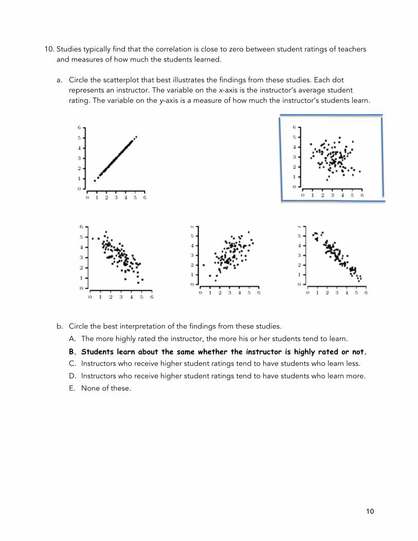
10. Studies typically find that the correlation is close to zero between student ratings of teachers and measures of how much the students learned.

a. Circle the scatterplot that best illustrates the findings from these studies. Each dot

represents an instructor. The variable on the x-axis is the instructor’s average student rating. The variable on the y-axis is a measure of how much the instructor’s students learn.

b. Circle the best interpretation of the findings from these studies.

A. The more highly rated the instructor, the more his or her students tend to learn.

B. Students learn about the same whether the instructor is highly rated or not. C. Instructors who receive higher student ratings tend to have students who learn less.

D. Instructors who receive higher student ratings tend to have students who learn more.

E. None of these.

11

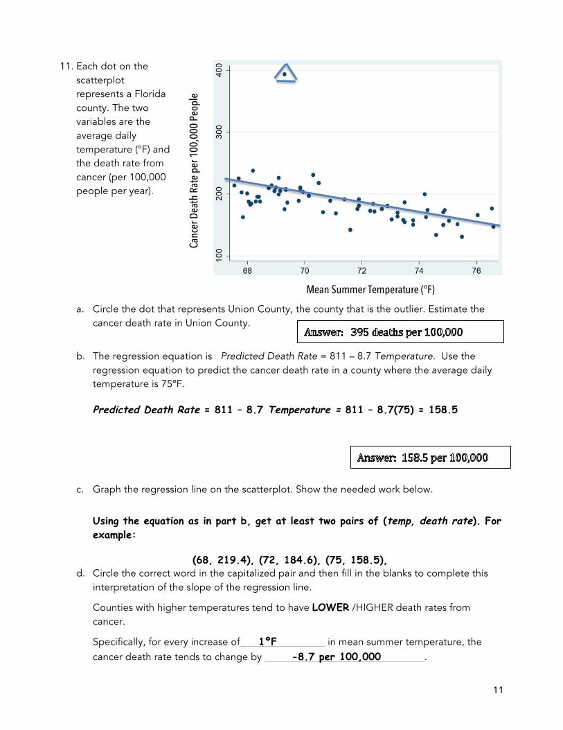
11. Each dot on the scatterplot represents a Florida county. The two variables are the average daily temperature (°F) and the death rate from cancer (per 100,000 people per year).

a. Circle the dot that represents Union County, the county that is the outlier. Estimate the cancer death rate in Union County.

b. The regression equation is Predicted Death Rate = 811 – 8.7 Temperature. Use the

regression equation to predict the cancer death rate in a county where the average daily temperature is 75ºF.

Predicted Death Rate = 811 – 8.7 Temperature = 811 – 8.7(75) = 158.5

c. Graph the regression line on the scatterplot. Show the needed work below.

Using the equation as in part b, get at least two pairs of (temp, death rate). For example:

(68, 219.4), (72, 184.6), (75, 158.5), d. Circle the correct word in the capitalized pair and then fill in the blanks to complete this

interpretation of the slope of the regression line.

Counties with higher temperatures tend to have LOWER /HIGHER death rates from cancer.

Specifically, for every increase of 1ºF in mean summer temperature, the cancer death rate tends to change by -8.7 per 100,000 .

Canc

er D

eath

Rat

e pe

r 100

,000

Peo

ple

per Y

ear

Mean Summer Temperature (°F)

12

Use this page for scratch paper—It won’t be graded.

13

Math 140 Formulas

sample mean: x =x∑

n

sample standard deviation: s =(x − x )2∑n −1

z-score: z = x − xs

interquartile range: IQR = Q3 – Q1

standard error of sampling distribution of p̂ : SE =p 1− p( )

n

standard error of sampling distribution of x : SE = σn

general confidence interval: observed value ± margin of error

confidence interval for p: p̂ ± m where m = z*⋅ p̂ 1− p̂( )

n

confidence interval for µ : x ± m where m = t * sn

general test statistic:

observed value− hypothesized valueSE

one-proportion z-test statistic: z = p̂ − p0

SE where SE =

p0 1− p0( )n

two proportion z-test statistic: z =p̂1 − p̂2( )− 0

SE

where SE = p̂ 1− p̂( ) 1n1

+ 1n2

⎛⎝⎜

⎞⎠⎟

and p̂ = number of successes in both samplesn1 + n2

14

t-test statistic for a mean: t = x − µSEEST

where SEEST =sn

two sample t-test statistic: t =x1 – x2( )− 0SEEST

where SEEST =s12

n1+s22

n2

chi-square statistic: χ 2 =O − E( )E

2

∑ where E =

row total( ) ⋅ column total( )grand total( )

correlation: r =1

n −1x − xsx

⎛⎝⎜

⎞⎠⎟

y − ysy

⎛

⎝⎜⎞

⎠⎟∑ =

1n −1

zx ⋅ zy∑

regression equation: predicted = a + bx

regression coefficients: b = r

sysy

a = y − bx

Calculator Commands

normalcdf(lower,upper,µ,σ )

invNorm(area,µ,σ )