Embed Size (px)
Citation preview
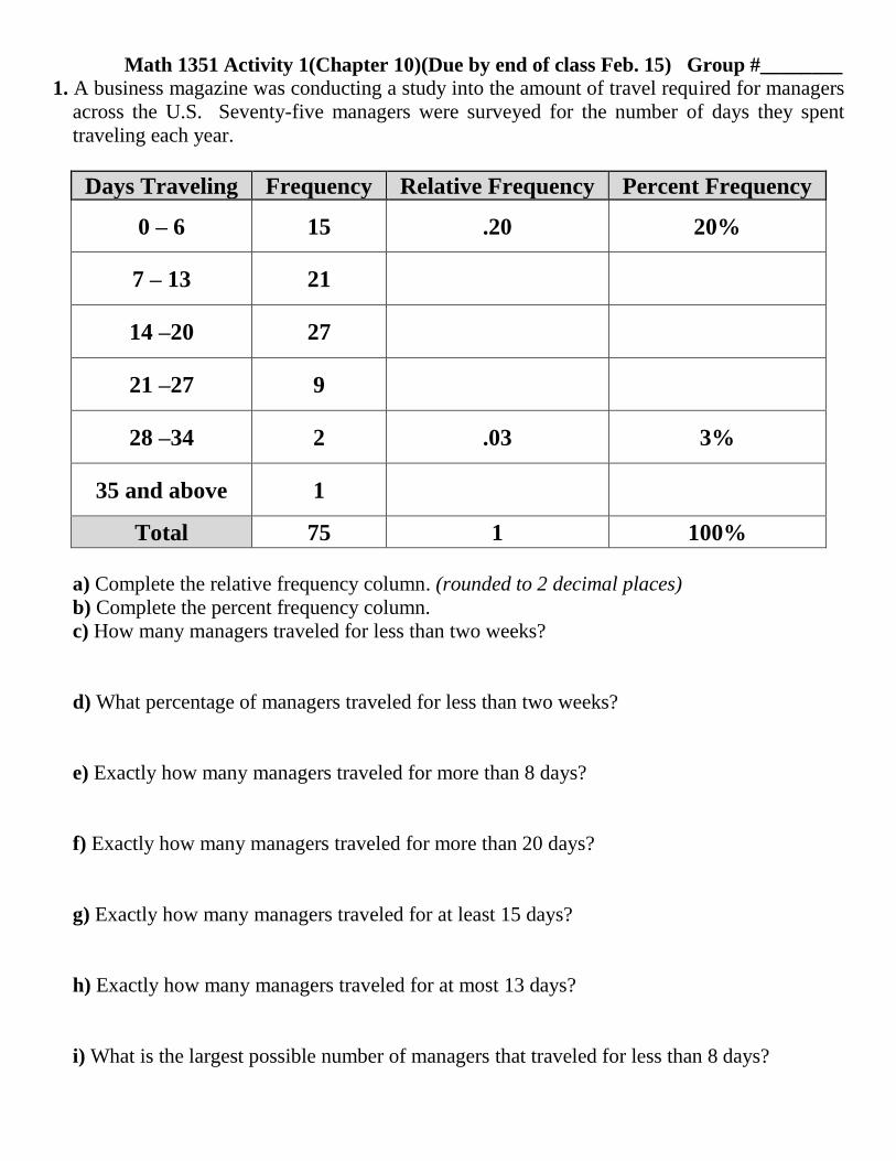
Math 1351 Activity 1(Chapter 10)(Due by end of class Feb. 15) Group #________
1. A business magazine was conducting a study into the amount of travel required for managers
across the U.S. Seventy-five managers were surveyed for the number of days they spent
traveling each year.
Days Traveling Frequency Relative Frequency Percent Frequency
0 – 6 15 .20 20%
7 – 13 21
14 –20 27
21 –27 9
28 –34 2 .03 3%
35 and above 1
Total 75 1 100%
a) Complete the relative frequency column. (rounded to 2 decimal places)
b) Complete the percent frequency column.
c) How many managers traveled for less than two weeks?
d) What percentage of managers traveled for less than two weeks?
e) Exactly how many managers traveled for more than 8 days?
f) Exactly how many managers traveled for more than 20 days?
g) Exactly how many managers traveled for at least 15 days?
h) Exactly how many managers traveled for at most 13 days?
i) What is the largest possible number of managers that traveled for less than 8 days?
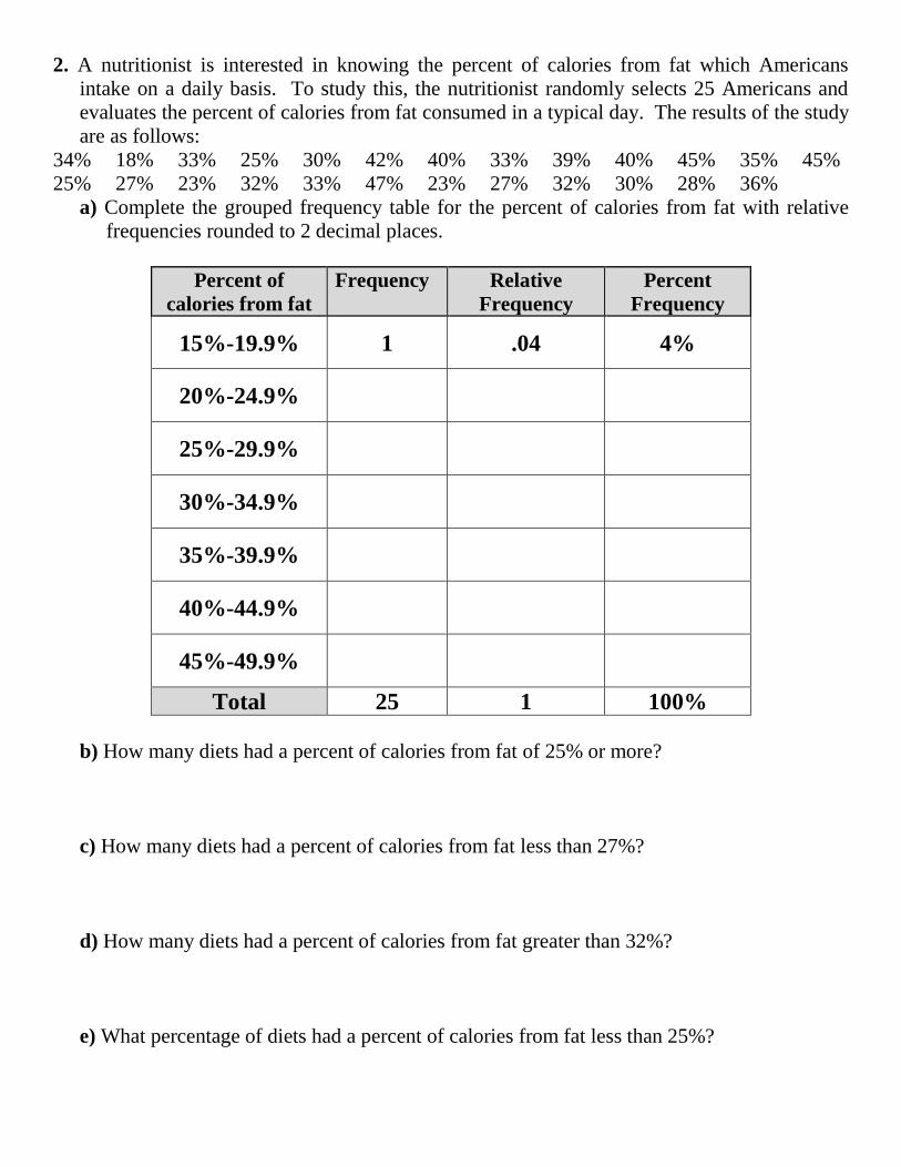
2. A nutritionist is interested in knowing the percent of calories from fat which Americans
intake on a daily basis. To study this, the nutritionist randomly selects 25 Americans and
evaluates the percent of calories from fat consumed in a typical day. The results of the study
are as follows:
34% 18% 33% 25% 30% 42% 40% 33% 39% 40% 45% 35% 45%
25% 27% 23% 32% 33% 47% 23% 27% 32% 30% 28% 36%
a) Complete the grouped frequency table for the percent of calories from fat with relative
frequencies rounded to 2 decimal places.
Percent of
calories from fat
Frequency Relative
Frequency
Percent
Frequency
15%-19.9% 1 .04 4%
20%-24.9%
25%-29.9%
30%-34.9%
35%-39.9%
40%-44.9%
45%-49.9%
Total 25 1 100%
b) How many diets had a percent of calories from fat of 25% or more?
c) How many diets had a percent of calories from fat less than 27%?
d) How many diets had a percent of calories from fat greater than 32%?
e) What percentage of diets had a percent of calories from fat less than 25%?
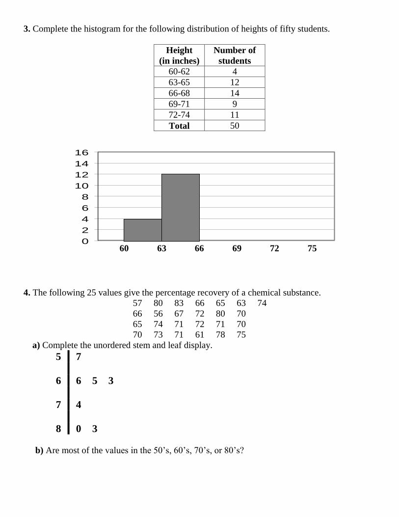
3. Complete the histogram for the following distribution of heights of fifty students.
Height
(in inches)
Number of
students
60-62 4
63-65 12
66-68 14
69-71 9
72-74 11
Total 50
4. The following 25 values give the percentage recovery of a chemical substance.
57 80 83 66 65 63 74
66 56 67 72 80 70
65 74 71 72 71 70
70 73 71 61 78 75
a) Complete the unordered stem and leaf display.
5 7
6 6 5 3
7 4
8 0 3
b) Are most of the values in the 50’s, 60’s, 70’s, or 80’s?
0
2
4
6
8
10
12
14
16
60 63 66 69 72 75
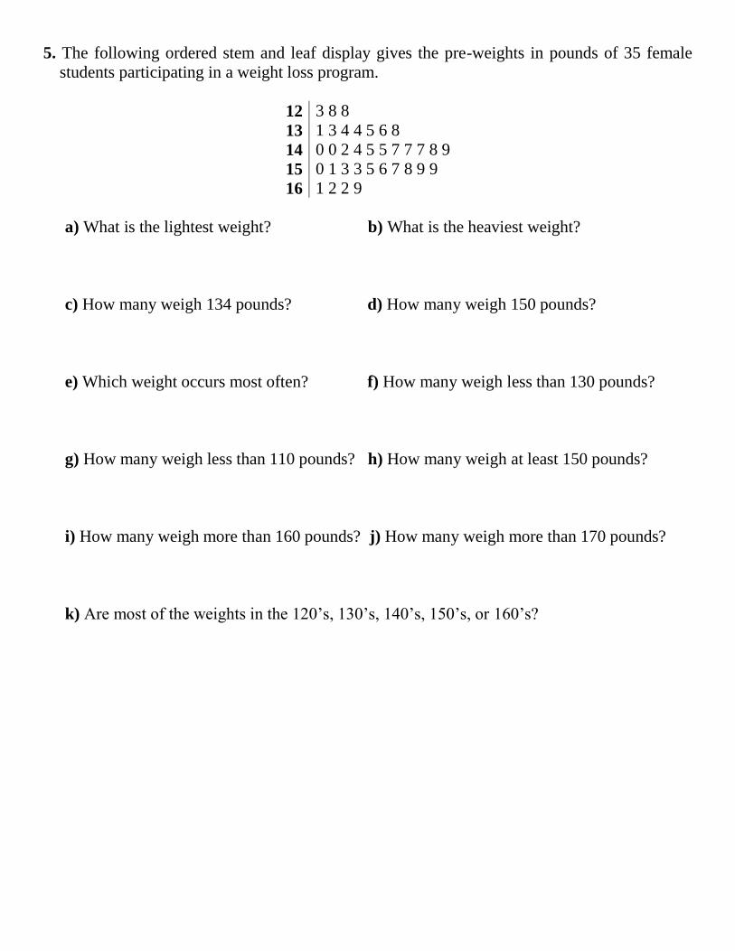
5. The following ordered stem and leaf display gives the pre-weights in pounds of 35 female
students participating in a weight loss program.
12 3 8 8
13 1 3 4 4 5 6 8
14 0 0 2 4 5 5 7 7 7 8 9
15 0 1 3 3 5 6 7 8 9 9
16 1 2 2 9
a) What is the lightest weight? b) What is the heaviest weight?
c) How many weigh 134 pounds? d) How many weigh 150 pounds?
e) Which weight occurs most often? f) How many weigh less than 130 pounds?
g) How many weigh less than 110 pounds? h) How many weigh at least 150 pounds?
i) How many weigh more than 160 pounds? j) How many weigh more than 170 pounds?
k) Are most of the weights in the 120’s, 130’s, 140’s, 150’s, or 160’s?

6. Stem-and-leaf plots can also be used to compare data sets. Here is a comparison of test
grades in an 8 AM math class and an 11 AM math class.
5 1 6 8 9
2
7 3 0 5 9
7 4 1 3 4 6 7 8 8
4 2 1 5 5 5 5 7 8 8
6 5 5 5 4 3 3 6 2 2 4 5 9
7 7 6 6 5 4 3 1 7 1 1 5
9 9 8 8 8 7 7 3 2 2 0 8 0 3
6 5 4 2 1 0 0 9
a) How many students scored in the 90’s in the 8 AM class?
b) How many students scored in the 90’s in the 11 AM class?
c) Which class did better on the test? Explain.
8 AM class 11 AM class
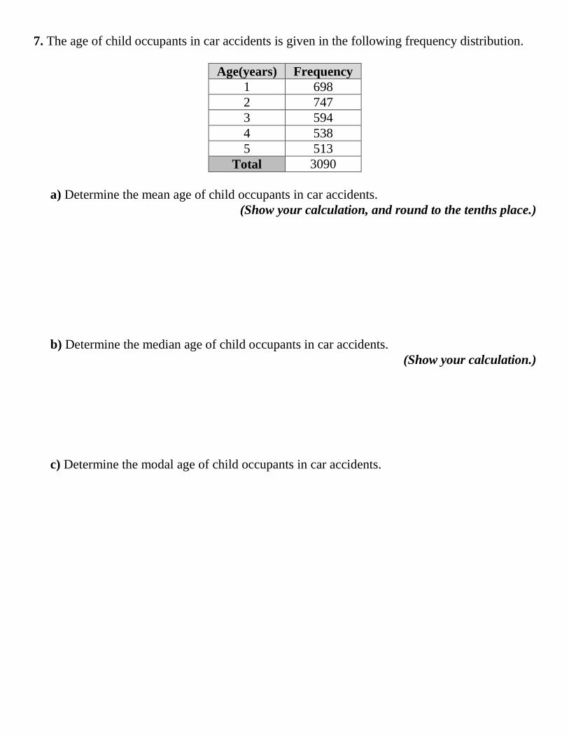
7. The age of child occupants in car accidents is given in the following frequency distribution.
Age(years) Frequency
1 698
2 747
3 594
4 538
5 513
Total 3090
a) Determine the mean age of child occupants in car accidents.
(Show your calculation, and round to the tenths place.)
b) Determine the median age of child occupants in car accidents.
(Show your calculation.)
c) Determine the modal age of child occupants in car accidents.
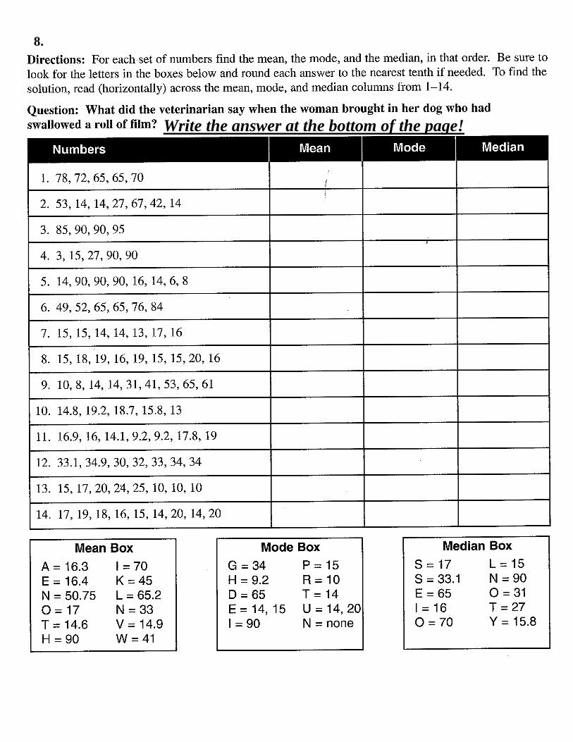
8.
Write the answer at the bottom of the page!
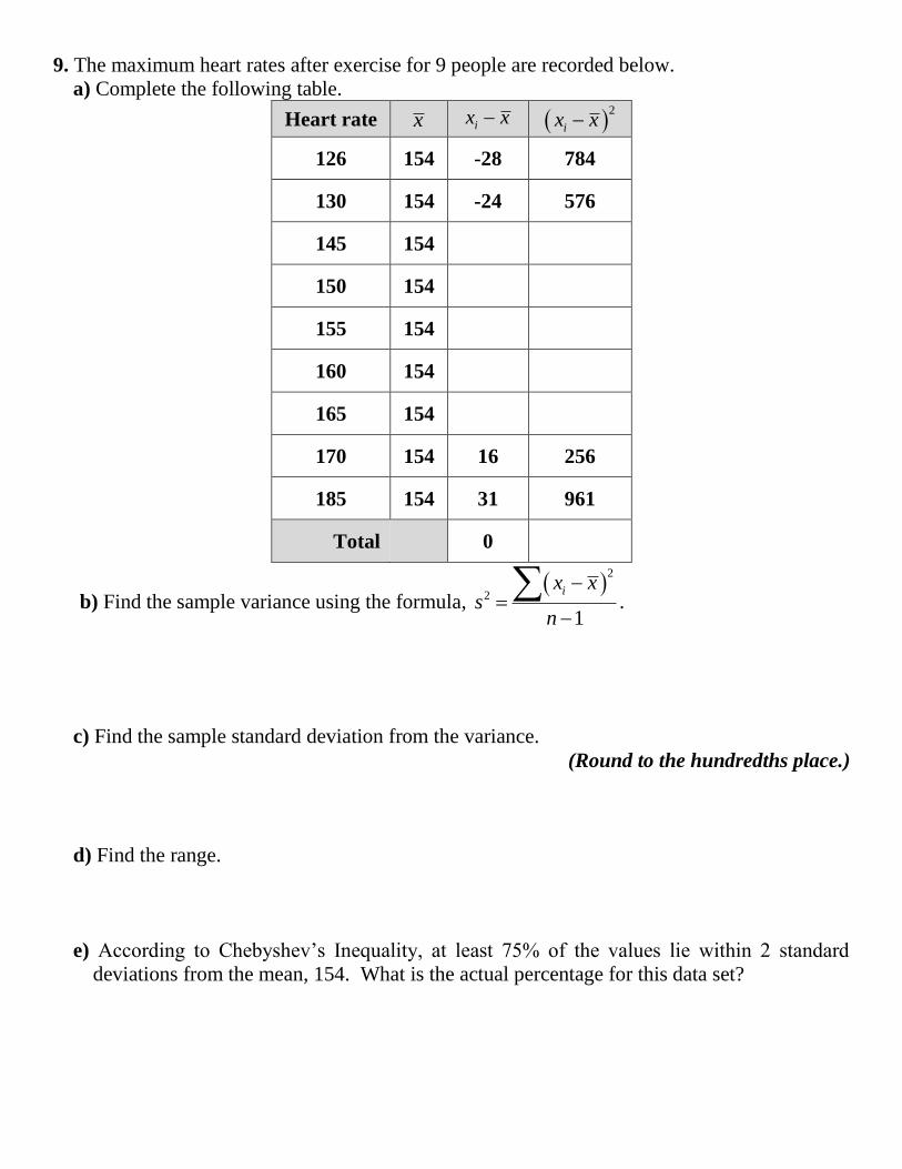
9. The maximum heart rates after exercise for 9 people are recorded below.
a) Complete the following table.
Heart rate x ix x 2
ix x
126 154 -28 784
130 154 -24 576
145 154
150 154
155 154
160 154
165 154
170 154 16 256
185 154 31 961
Total 0
b) Find the sample variance using the formula,
2
2
1
ix xs
n
.
c) Find the sample standard deviation from the variance.
(Round to the hundredths place.)
d) Find the range.
e) According to Chebyshev’s Inequality, at least 75% of the values lie within 2 standard
deviations from the mean, 154. What is the actual percentage for this data set?
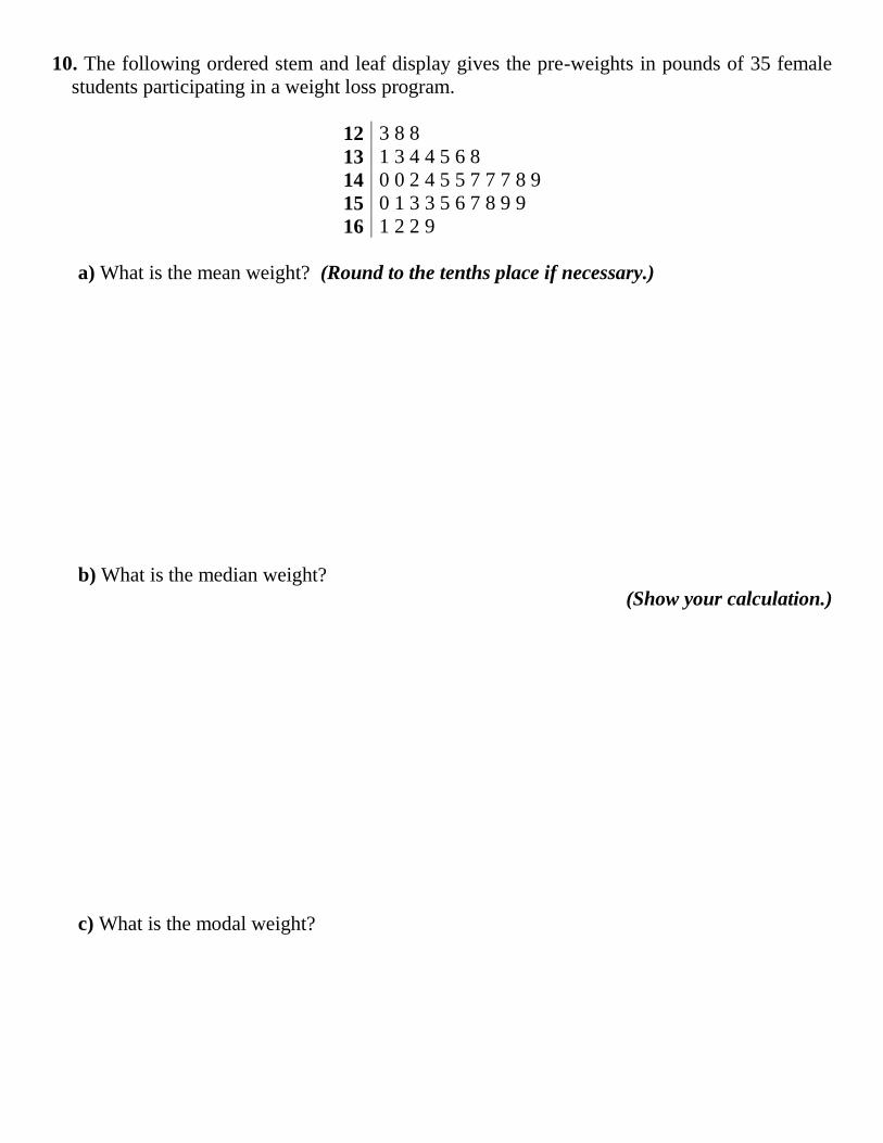
10. The following ordered stem and leaf display gives the pre-weights in pounds of 35 female
students participating in a weight loss program.
12 3 8 8
13 1 3 4 4 5 6 8
14 0 0 2 4 5 5 7 7 7 8 9
15 0 1 3 3 5 6 7 8 9 9
16 1 2 2 9
a) What is the mean weight? (Round to the tenths place if necessary.)
b) What is the median weight?
(Show your calculation.)
c) What is the modal weight?
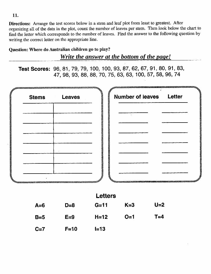
11.
Write the answer at the bottom of the page!
12. For the data set: 1,1,3,39 ,
a) Determine the mean. b) Determine the median.
If the extreme value of 39 is changed to 7, leading to the new data set: 1,1,3,7 ,
c) Determine the new mean. d) Determine the new median.
e) Which measure of central tendency was more resistant to the change in the extreme value
in this situation?
13. For the data set: 1,1,1,7,7,19 ,
a) Determine the median. b) Determine the mode.
If one of the extreme values of 1 is changed to 0, and the extreme value of 19 is changed to
7, leading to the new data set: 0,1,1,7,7,7 ,
c) Determine the new median. d) Determine the new mode.
e) Which measure of central tendency was more resistant to the change in the extreme values
in this situation?
14. According to Chebyshev’s Inequality, at least 36% of the values in a data set must lie within
1.25 standard deviations from the mean. The percentage from the inequality is usually
smaller than the actual percentage for the data set. Determine the exact percentage of
values that lie within 1.25 standard deviations from the mean for the following data sets.
a) 1,2,3,4,5,6,7,8,19,20 , 7.5x , 6.69s
b) 4,5,15,16,17,18,19,20,33,40 , 18.7x , 11.00s
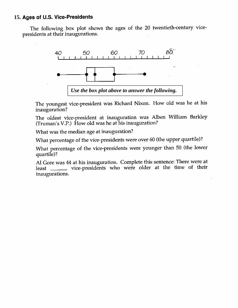
15.
Use the box plot above to answer the following.
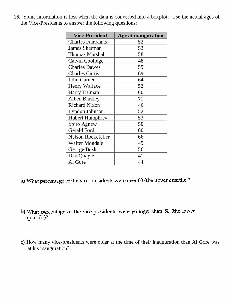
16. Some information is lost when the data is converted into a boxplot. Use the actual ages of
the Vice-Presidents to answer the following questions:
Vice-President Age at inauguration
Charles Fairbanks 52
James Sherman 53
Thomas Marshall 58
Calvin Coolidge 48
Charles Dawes 59
Charles Curtis 69
John Garner 64
Henry Wallace 52
Harry Truman 60
Alben Barkley 71
Richard Nixon 40
Lyndon Johnson 52
Hubert Humphrey 53
Spiro Agnew 50
Gerald Ford 60
Nelson Rockefeller 66
Walter Mondale 49
George Bush 56
Dan Quayle 41
Al Gore 44
a)
b)
c) How many vice-presidents were older at the time of their inauguration than Al Gore was
at his inauguration?
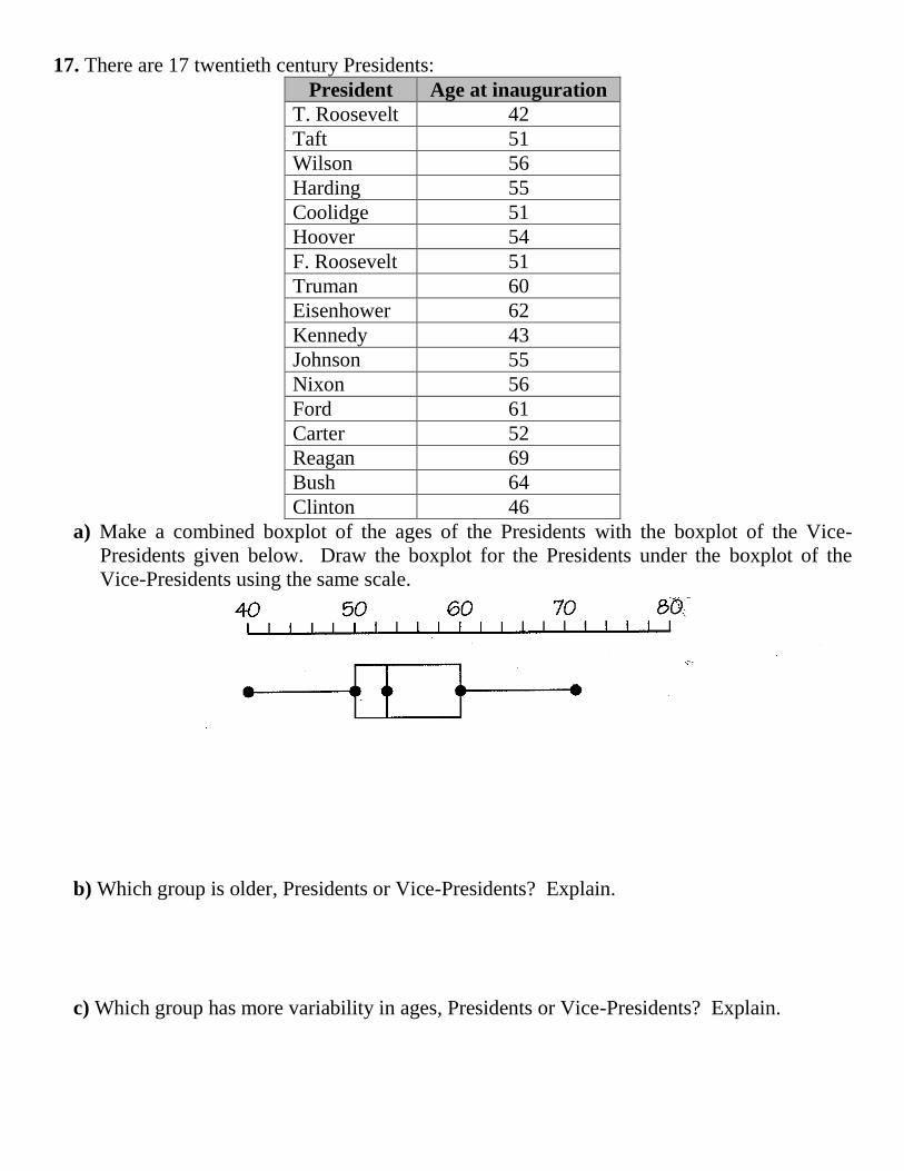
17. There are 17 twentieth century Presidents:
President Age at inauguration
T. Roosevelt 42
Taft 51
Wilson 56
Harding 55
Coolidge 51
Hoover 54
F. Roosevelt 51
Truman 60
Eisenhower 62
Kennedy 43
Johnson 55
Nixon 56
Ford 61
Carter 52
Reagan 69
Bush 64
Clinton 46
a) Make a combined boxplot of the ages of the Presidents with the boxplot of the Vice-
Presidents given below. Draw the boxplot for the Presidents under the boxplot of the
Vice-Presidents using the same scale.
b) Which group is older, Presidents or Vice-Presidents? Explain.
c) Which group has more variability in ages, Presidents or Vice-Presidents? Explain.
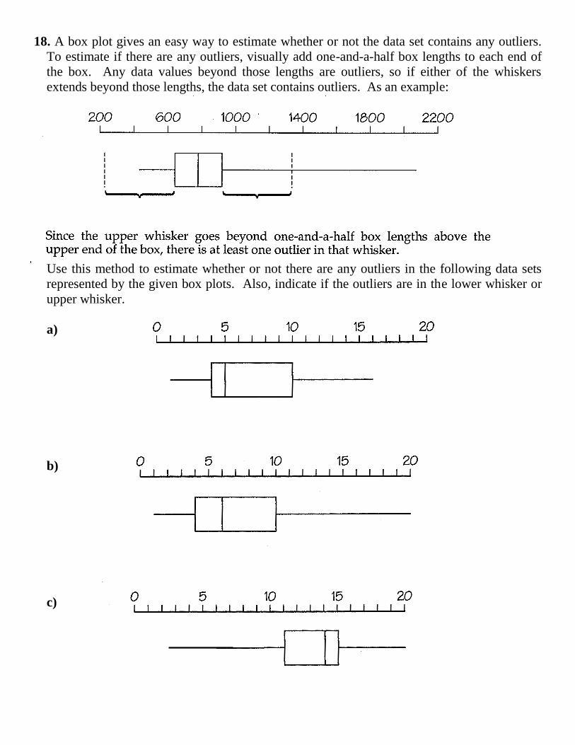
18. A box plot gives an easy way to estimate whether or not the data set contains any outliers.
To estimate if there are any outliers, visually add one-and-a-half box lengths to each end of
the box. Any data values beyond those lengths are outliers, so if either of the whiskers
extends beyond those lengths, the data set contains outliers. As an example:
Use this method to estimate whether or not there are any outliers in the following data sets
represented by the given box plots. Also, indicate if the outliers are in the lower whisker or
upper whisker.
a)
b)
c)
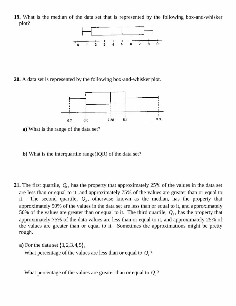
19. What is the median of the data set that is represented by the following box-and-whisker
plot?
20. A data set is represented by the following box-and-whisker plot.
a) What is the range of the data set?
b) What is the interquartile range(IQR) of the data set?
21. The first quartile, 1Q , has the property that approximately 25% of the values in the data set
are less than or equal to it, and approximately 75% of the values are greater than or equal to
it. The second quartile, 2Q , otherwise known as the median, has the property that
approximately 50% of the values in the data set are less than or equal to it, and approximately
50% of the values are greater than or equal to it. The third quartile, 3Q , has the property that
approximately 75% of the data values are less than or equal to it, and approximately 25% of
the values are greater than or equal to it. Sometimes the approximations might be pretty
rough.
a) For the data set 1,2,3,4,5 ,
What percentage of the values are less than or equal to 1Q ?
What percentage of the values are greater than or equal to 1Q ?
b) For the data set 1,1,1,4,5,6 ,
What percentage of the values are less than or equal to 3Q ?
What percentage of the values are greater than or equal to 3Q ?
c) For the data set 1,1,1,1,1,1,1 ,
What percentage of the values are less than or equal to 2Q ?
What percentage of the values are greater than or equal to 2Q ?
d) For the data set 1,2,3,4,5,6,7,8 ,
What percentage of the values are less than or equal to 1Q ?
What percentage of the values are greater than or equal to 2Q ?
What percentage of the values are greater than or equal to 3Q ?
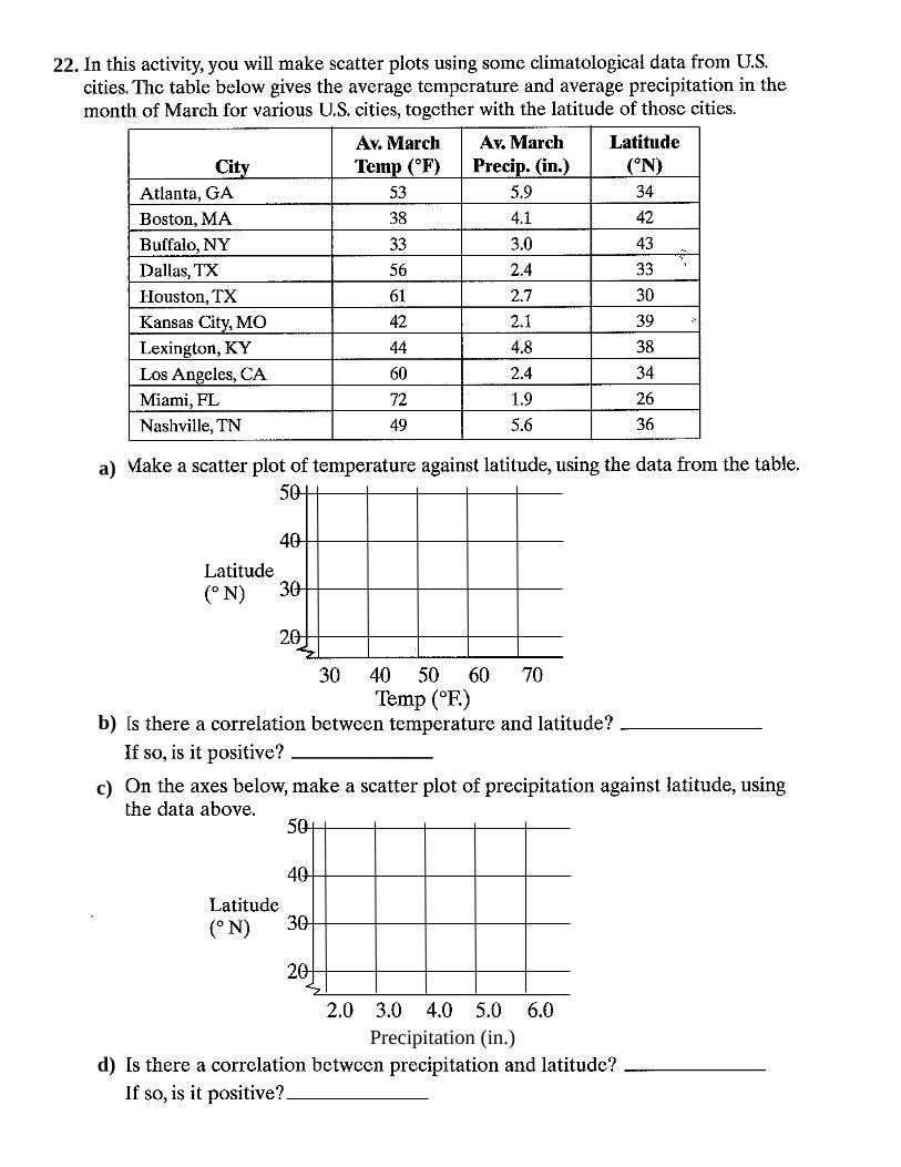
22.
a)
b)
c)
d)
Precipitation (in.)
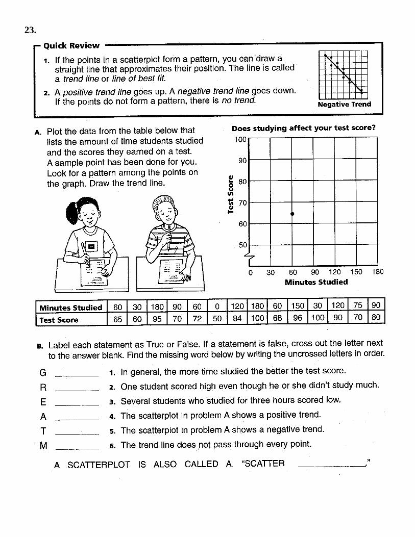
23.
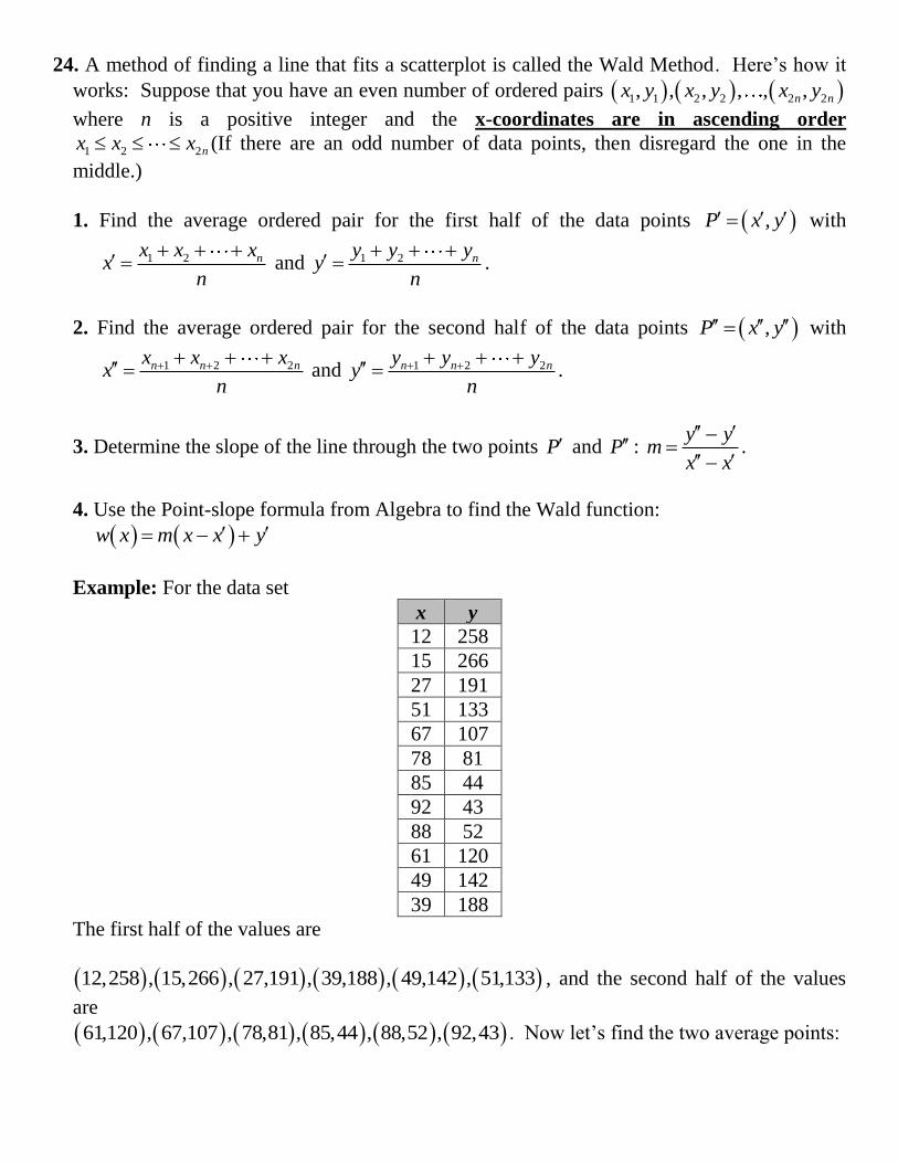
24. A method of finding a line that fits a scatterplot is called the Wald Method. Here’s how it
works: Suppose that you have an even number of ordered pairs 1 1 2 2 2 2, , , , , ,n nx y x y x y
where n is a positive integer and the x-coordinates are in ascending order
1 2 2nx x x (If there are an odd number of data points, then disregard the one in the
middle.)
1. Find the average ordered pair for the first half of the data points ,P x y with
1 2 nx x xx
n
and 1 2 ny y y
yn
.
2. Find the average ordered pair for the second half of the data points ,P x y with
1 2 2n n nx x xx
n
and 1 2 2n n ny y y
yn
.
3. Determine the slope of the line through the two points P and P : y y
mx x
.
4. Use the Point-slope formula from Algebra to find the Wald function:
w x m x x y
Example: For the data set
x y
12 258
15 266
27 191
51 133
67 107
78 81
85 44
92 43
88 52
61 120
49 142
39 188
The first half of the values are
12,258 , 15,266 , 27,191 , 39,188 , 49,142 , 51,133 , and the second half of the values
are
61,120 , 67,107 , 78,81 , 85,44 , 88,52 , 92,43 . Now let’s find the two average points:
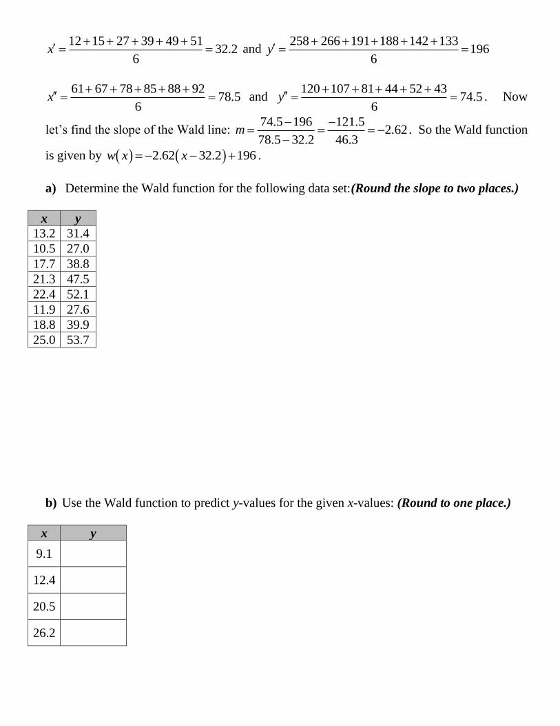
12 15 27 39 49 5132.2
6x
and
258 266 191 188 142 133196
6y
61 67 78 85 88 9278.5
6x
and
120 107 81 44 52 4374.5
6y
. Now
let’s find the slope of the Wald line: 74.5 196 121.5
2.6278.5 32.2 46.3
m
. So the Wald function
is given by 2.62 32.2 196w x x .
a) Determine the Wald function for the following data set:(Round the slope to two places.)
x y
13.2 31.4
10.5 27.0
17.7 38.8
21.3 47.5
22.4 52.1
11.9 27.6
18.8 39.9
25.0 53.7
b) Use the Wald function to predict y-values for the given x-values: (Round to one place.)
x y
9.1
12.4
20.5
26.2
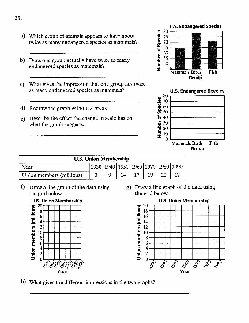
25.
a)
b)
c)
d)
e)
f) g)
h)
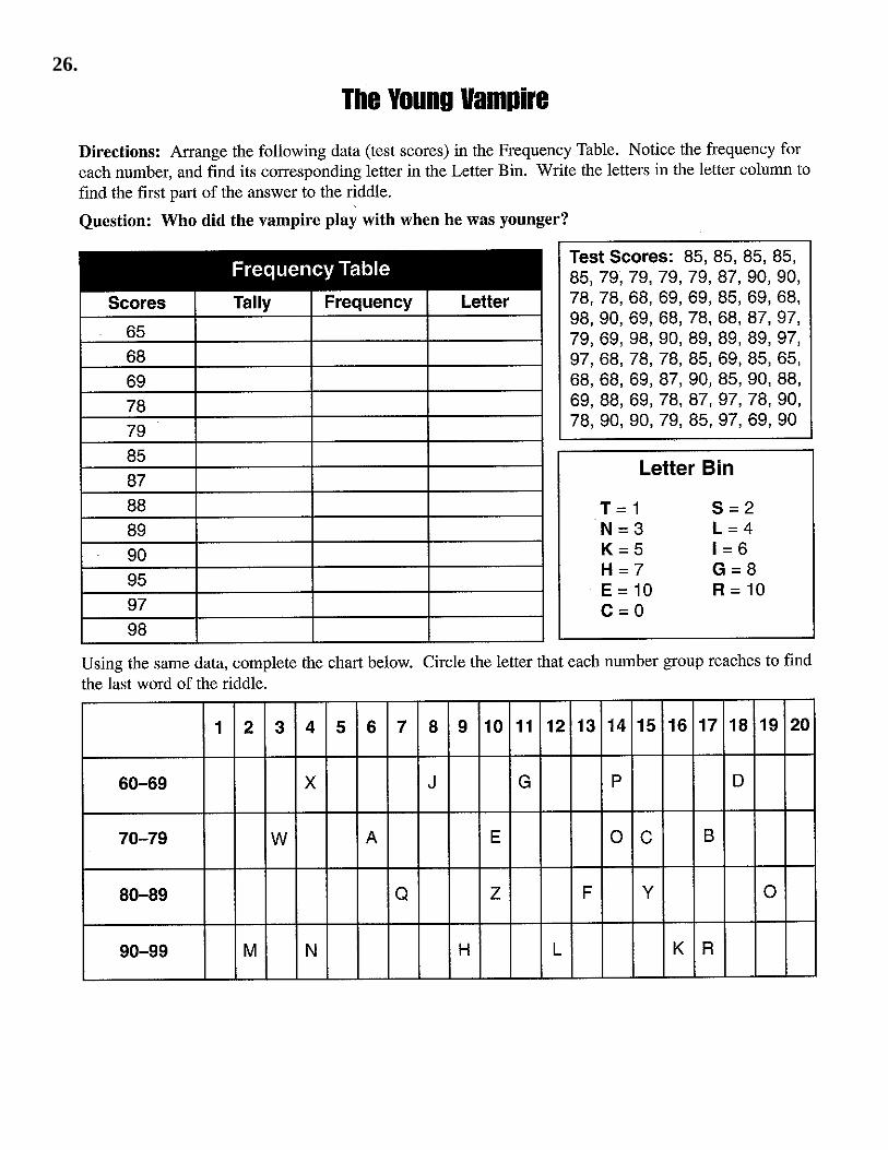
26.