(NASA-CR-137980) PERTURBATION THEORY OF N74-20128STRUCTURE IN CLASSICAL LIQUID MIXTURES:APPLICATION TO METALLIC SYSTEMS NEARPHASE SEPARATION Ph.D. Thesis (Cornell UnclasUniv.) '54 p HC $10.75 CSCL 11F G3/17 33471

Materials Science Center

Cornell UniversiITHACA, NEW YORK

14850

https://ntrs.nasa.gov/search.jsp?R=19740012015 2018-05-28T20:35:25+00:00Z

Report #2154

PERTURBATION THEORY OF STRUCTURE

IN CLASSICAL LIQUID MIXTURES:

APPLICATION TO METALLIC SYSTEMS

NEAR PHASE SEPARATION

byRobert Lloyd Henderson

Ph.D. Thesis Research Group:January 1974 Prof. N. W. Ashcroft

LASSP

ACKNOWLEDGMENTS

The author wishes to thank Professor Neil Ashcroft for

his guidance, encouragement, and patience as thesis advisor,

and for his steady contributions of time and ideas to this

work.

Important contributions to the progress of this work

have been made by David Stroud, to whom the author is indebted

for a significant discussion at the outset, and Myron Mandell,

who taught the author the ways of computers.

Discussions with postdocs and fellow students have pro-

vided a constant source of ideas and perspective. For such

discussions, the author especially thanks Andreas Bringer,

Mark Huberman, James Hammerberg, and Myron Mandell.

The author thanks his father and mother for the sacri-

fices they have made for his education, and for their constant

support and encouragement.

Finally, the author thanks his son David for patience,

and his wife Karen for patience, love, and stubborn support,

without which this job simply could not have been done.

This work was supported by the National Aeronautics and Space

Administration and the National Science Foundation through the

Materials Science Center at Cornell University.

PRECEDING PAGE BLANK NOT FILMIiL)

-iv-

TABLE OF CONTENTS

I. Introduction and Statement of the Problem ............. 1

II. General Discussion and Mean Field Theory............. 19

III. The Formal Development...............................33

1 1IV. Approximate Solutions for the f. and a .. .... .... . 5 8

V. Application to Liquid Metal Systems ................. 74

VI. Discussion, Conclusions, and Suggestions

for Further Work ................................. .. 120

Appendix A: The Distribution Functions ................... 128

Appendix B: Phase Separation and Singularities

in the Sij (k) ................................ 132

Appendix C: The k = 0 Result (4-32)......................135

Appendix D: The MDA to f (k) for aij

Two-component Fluid ............................ 140

References...............................................143

-v-

LIST OF TABLES

Table I: Results at k = 0, T = TM for the pure

alkalis in MDA ................................ 89

Table II: Comparison of MF and MDA calculations

of f1 (0) in Li-Na ................... ........ 101

Table III: Results of the variational calculation

for Li-Na........................................................104

Table IV: Results in MDA for D(y) at y 3 0.............. 109

-vi-

LIST OF FIGURES

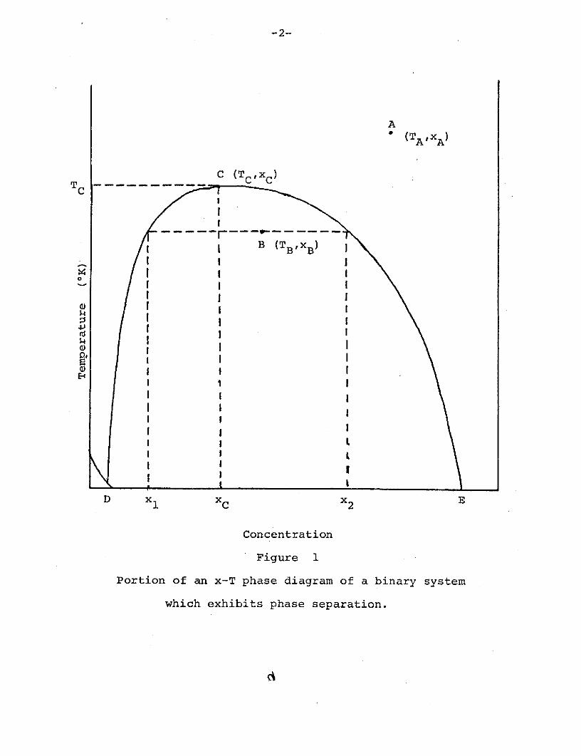
Figure 1: Portion of an x-T phase diagram of a binary

system which exhibits phase separation .......... 2

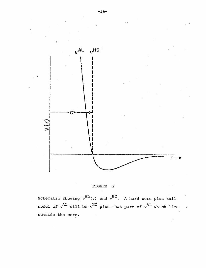
Figure 2: Schematic showing v A L (r) and v HC (r). A

hard core plus tail model of vAL will be vHC

ALplus that part of v which lies outside

the core...................................... 16

Figure 3: Comparison of experimental phase boundary

and MF line of singularities in Li-Na. The

parameters of the MF calculation are

specified in the text.......................... 81

Figure 4a: S HC(y) in PY for n = .456.

4b: DMF(Y) = 1 + pS HC(y)fF(y) for Na

at T = 371 0K..................................83

Figure 5: fl(y) in MDA for Na, Li, and K................. 92

Na Na 0Figure 6: SMDA(0) vs. for rNa 4.064, r .884 A....96

Figure 7: Comparison of line of singularities

calculated in MF and MDA with identical

parameters ..................................... 99

Figure 8: The a-n plane at T = 575 0 K, x = .4,

in Li-Na. The denominator D is greater

than zero above the line and less than

zero below .... .................. ........ 106

Figure 9: Log-log plot of D(y) in MDA for Li-Na at

x = .4, T = 5750 K, a = .825 and n = .430......110

-vii-

Figure 10: Log-log plot of D(y)-D(O) in MDA for Li-Na

at x = .4, T = 5750 K, a = .825 and n = .430...111

Figure 11: Partial structure factors for Li-Na at

x = .4, T = 5750 K, a = .825, and n = .430.

The solid lines represent the structure in

in the MDA, and the dashed lines represent the

structure of the hard sphere reference

system ........................................ 113

Figure B-l: Gibbs energy per particle as a function

of concentration at T = T1 < TC ............... 133

-viii-

ABSTRACT

This work concerns the partial structure factors of

classical simple liquid mixtures near phase separation. The

theory is developed for particles interacting through pair

potentials, and is thus appropriate both to insulating fluids,

and also to metallic systems if these may be described by an

effective ion-ion pair interaction. The motivation arose

from consideration of metallic liquid mixtures, in which

resistive anomalies have been observed near phase separation.

ref 1 refThe pair potential is written as v.. = v.. + v.., where v..

is the pair interaction appropriate to a reference fluid and

is chosen so that v.. may be treated as a perturbation. We

study how to correct a mean field theory appropriate to such a

potential for the effects of correlated motions in the

reference fluid. The work is cast in terms of functions fij

which are closely related to the direct correlation functions

of Ornstein and Zernike. Exact equations for the fij are

derived by a method, originally developed for the study of

the quantum.electron gas, which treats the densities of the

FI)II k

mixture as basic variables in a linear response problem. We

obtain approximate solutions to these equations which, however,

are exact to first order in v.. in the long wavelength limit,

and which explicitly include the effects of reference system

correlations. These solutions are then used to calculate the

long wavelength form of the structure factors of metallic

refalloys, where we select for v.. the potentials appropriate to

a mixture of hard spheres. We seek to observe the singular-

ities, at k = 0, associated with phase separation (in the

critical region) and the long wavelength behavior which

accompanies these singularities. The results are qualita-

tively in accord with our physical expectations. Quantitative

agreement with experiment seems to turn on the selection of

the hard core reference potential in terms of the metallic

effective pair potential, a task for which a successful

systematic procedure has yet to be found. It is suggested

that the present effective pair potentials are perhaps not

properly used to calculate the metallic structure factors at

long wavelength. Suggestions are made for application of

these results to the thermodynamic and structural properties

of insulating fluids. In the case of metallic systems, a

qualitative explanation of the resistive anomaly is proposed,

and suggestions made for a quantitative test of the hypothesis.

I. Introduction and Statement of the Problem

The work reported here arose from consideration of a

single experimental result, the resistance anomaly observed

in some binary liquid metal alloys as the phase separation

temperature is approached. The importance of this result is

that the theoretical difficulty it presents has its origin

in a central problem of the theory of classical liquids,

namely, the calculation of liquid structure from the

interactions among the particles of the liquid. In this

section, we shall describe these experiments and develop

our analysis of these experiments to the point where a clear

statement of the problem and program of this thesis can be

made.

I-A. Phase Separation and the Experiment of Schirmann

and Parks

To set the stage, we must begin with a recital of the

basic facts of phase separation in binary systems. Consider

a binary system composed of N1 particles of type 1 and N2

particles of type 2. The thermodynamic state of this

system may be considered a function of three variables;

pressure p, temperature T, and concentration x = N2/(N 1 + N).

The phase diagram relevant to this work is that formed, at

constant p, in the x-T plane. Fig. 1 represents schematically

a portion of an x-T diagram of the type important to our work.

It represents, in fact, an abstraction from the x-T diagram

-1-b

-2-

A

• (TA, xA

C (T,(T Xc XB)

1 I

s-

I I I

I I I

Figure 1

Portion of an x-T phase diagram of a binary system

which exhibits phase separation.

which exhibits phase separation.

-3-

compiled by Schurmann (1971) for the Li-Na system.

The phase diagram specifies, for each point (x,T), the

stable configuration of the corresponding mixture. In Fig. 1,

points from the small triangular region at the lower left

correspond to a solid phase. The phase boundary from D to

E separates the remainder of the region shown into two

liquid phases. For a point above the boundary, say the point

A specified by (XA,TA), the stable configuration is a single,

uniformly mixed, alloy of concentration xA. For a point

below the boundary, say the point specified by (XB,TB), the

stable configuration is a separated phase. In this phase,

two distinct alloys are present simultaneously. (Under the

influence of gravitation, these alloys will occupy two

separate regions of the container, divided by a meniscus.)

These alloys are described by concentrations xl < xB and

x2 > xB' where xl and x2 are determined by TB alone as the

concentrations at which the phase boundary cuts the line

T = TB. This construction is illustrated in Fig. 1. The

relative amounts of these two alloys are determined from xl

and x2, the given XB , and the requirement that all particles

be accounted for.

At points above the phase boundary, where a single

uniform alloy can be maintained at equilibrium, the components

are said to be miscible. The boundary defines a critical

temperature TC above which the components are miscible in all

proportions. The point C at which the line T = TC intersects

the phase boundary is the critical point, and defines a

-4-

critical concentration xC. TC and xC are indicated in Fig. 1.

The transition of an alloy from the uniform to the separated

phase is known as phase separation.

The experiments which motivated this work are concerned

with what happens in the stable uniform alloy at temperatures

just above phase separation. Schiirmann and Parks (1971) have

measured the electrical resistance as a function of

temperature at various concentrations in two metallic binary

systems, Li-Na and Ga-Hg. As we shall outline shortly, the

electrical resistance provides an integrated measure of

fluctuation effects. The purpose of these experiments was

to determine if changes in the fluctuation spectrum would

cause the resistance to show any precursive behavior, that

is, to respond in an observable way as phase separation is

approached. Such a response might be considered analogous

to the critical opalescence of the critical liquid-gas system.

No precursive behavior was observed at any concentration

in the Ga-Hg system. In the Li-Na system, some degree of

precursive behavior appeared at most concentrations, and the

effect became more pronounced as the concentration varied

toward the critical value. The effect takes the following

form. If the temperature is decreased, starting at a point

well removed from phase separation, the resistance decreases

at first in a nearly linear fashion. As the temperature of

separation is approached, however, the resistance begins to

decrease more rapidly, so that a plot of resistance vs. T

develops a pronounced curvature, and the resistance attains

-5-

a value at separation which lies below the linear

extrapolation of the high temperature results.

I-B. The Resistance Anomaly and Liquid Structure

To understand the significance of these experiments, we

consider first the theory of conduction in liquid metal

alloys. The simplest successful theory was proposed for the

case of a pure fluid by Ziman (1961). The theory was

generalized to the case of binary alloys by Ziman and Faber

(1965). The development of the theory has been aided by the

introduction of adequate models for the electron-ion

pseudopotential and the liquid structure. Calculations for

pure simple liquid metals (Ashcroft and Lekner, 1966) and for

liquid binary alloys of simple metals (Ashcroft and Langreth,

1967, A, B, to be referred to as Al-I and Al-II respectively)

have achieved reasonable agreement with experiment. Although

this success remains something of a mystery, we base our

analysis on the Ziman theory. The theory, as we shall see,

encompasses, in a reasonable way, the possibility of an

anomaly near phase separation.

In the formulation of Al-II, the result of the Ziman and

Faber theory for the resistivity of a binary alloy is written

Pelec e2k 4 Z* dy y3{2x(l-x) S12 (Y)V1(Y)v2(Y)

2 2 k

+ xS11() (v(y))2 + (1-x)S 2 2 (Y) (v 2 (y)) 2}. (1-1)

For this discussion, we need not give careful definitions to

-6-

most of the pieces of this expression. The liquid metal is

viewed as a system of rigid ion cores, of types one and two,

moving about in a sea of nearly free conduction electrons.

Defined relative to this model, kF is the usual Fermi wave

vector, Z* is a (concentration dependent) effective valence,

x is the concentration variable we have already defined, y is

a wave number variable measured in units of 2kF, and the

functions vi(y) are dimensionless form factors for the

screened electron-ion interactions. The key functions of

our work are the functions S..(y), the partial structure

factors, for they are the only functions in (1-1) which

contain detailed information on the ionic positions. They

are defined by

S..(k) = (NiNj ) <i (k) .j (-k)> - (NiNj ) 6 . (1-2)13- 1 1 - - 1 0 k,O

Here, N1 and N2 are the particle numbers defined above, < >

denotes a thermal average, and the operators i(k) are

defined by

ik-rii(k) = e (1-3)

m

where ri denotes the position of the mth particle of type i.-m

The operators i(k) have the property that

Pi(k) = < , (k) > , (1-4)

thwhere Pi(k) is the kth Fourier coefficient of the equilibrium

density of particles of type i. From (1-2), we see that the

S..ij(k) represent the static density fluctuation spectrum of

-7-

the liquid. It is reasonable to expect the density

fluctuations to reflect in some way the nearness of the

phase separation instability. This idea provided the

original motivation for the resistivity measurements, and

lies at the heart of our work.

It will be useful in this work to present here a few more

relations involving the structure factors. A more detailed

discussion of such matters is reserved for an appendix (A)

on the classical n-body distribution functions.

Many of the general points we need to make can be made

in reference to pure fluids, avoiding the clutter of notation

introduced by consideration of binary systems. For a pure

fluid, we can define a single static structure factor S(k) by

ik•(r -rm)S(k) = <Ce > - N k, (1-5)

N k,0nm

where N is the number of particles and r denotes the position-n

of the nth particle. This function is related by Fourier

transform to the radial distribution function g(r):

V -k -ik.rg(r) = 1 + e (S(k) - 1) , (1-6)

where V is the volume of the system. The function g(r) is

proportional to the conditional probability that a particle

will be found at r, given a particle at the origin. Finally,

the functions S(k) and g(r) are related to the two body

distribution function p2 (r,r'). This function has the property

*The integral in this equation, incidently, defines theFourier transform convention which we adopt throughout thiswork.

-8-

that P 2 (,r')dr dr' is the probability of finding simulta-

neously one particle in the volume element dr about r and

another in the element dr' about r'. In the translationally

invariant system, p2 (r,r') = p2 (r-r') and

g(r) = (V/N) P2 (r) . (1-7)

The generalization of (1-6) to binary systems is

r dkj(r) = 1 + e i - (s (k) - 6 .) , (1-8)

ij 2 T) 33

where gij (r) now represents, suitably normalized, the

probability of finding a particle of type j at a distance

r from a given particle of type i. Clearly, gij (r) = g ji(r).

The generalization of (1-7) is straightforward.

We can collect what has been said so far into a first

statement of the problem of this work. That problem is to

calculate the partial static structure factors of the alloy

with sufficient precision that the onset of phase separation

can be observed and the resistance anomaly explained.

I-C. Expectations

The development of our approach has been guided to a

considerable extent by our expectations for the form of the

outcome.

The first, and most important, of these expectations

concerns the limit as k->O, and takes the following form.

At all points (x,T), we can in principle calculate the

-9-

structure factors of the uniform phase. (For this purpose,

points below the phase boundary are exceptional only in that

the appropriate Gibbs energy is higher than that of some

separated phase.) A thermodynamic analysis (outlined in

appendix B) shows that such calculations will yield, at each

concentration, a temperature at which the partial structure

factors will diverge as k->O. When plotted vs. concentration,

these temperatures will form a curve suggesting, but not

strictly reproducing, the phase boundary. This curve lies in

general below the phase boundary, rising to join it at only

one point, the critical point. We shall seek to calculate

this line of hypothetical singularities at k = 0, and identify

its highest point as the critical point.

A second guide in this work has been a conjecture that

it is the small k behavior associated with this k = 0

singularity which gives rise to the resistance anomaly. As

this conjecture is at variance with that of Schirmann and

Parks (1971), we should outline the manner in which the small

k behavior might account for the observed effects. First, in

the resistance data for the Li-Na system, some degree of

*This conjecture is also at variance with that of Fisher andLanger (1968), who suggest that the observed resistanceanomalies at magnetic critical points must not be due to longrange correlations, because of the finite mean free path ofthe conduction electrons. Their point, however, is that theelectron mean free path is limited by scattering other thanspin scattering (e.g. phonons, impurities), while for theliquid metal alloy, we consider that the only scatteringpresent is the scattering from density fluctuations treatedin the Ziman formula. The electrons may thus be scatteredby even long wavelength fluctuations.

-10-

anomalous behavior is observed at most concentrations, but

the effect clearly becomes more pronounced as the concen-

tration is varied toward the critical value. This observation

seems to reflect the relation, described above, between the

phase boundary and the line of singularities.

Secondly, we must ask why the effect is observed in

Li-Na but not in Ga-Hg. Consider the form of (1-1). The

upper limit on the integral is 2kF, which depends on the

effective valence of the alloy. Now the partial structure

factors are characterized by strong first peaks (AL-II), and

the valence dependence of the integration limit is such that

these peaks lie within the range of integration for Ga-Hg,

but just outside it for Li-Na. Thus, when we observe that

large k effects are heavily weighted by the factor y3 , it is

reasonable that a small k effect will be lost in Ga- Hg, but

(barely) observable in Li-Na. We note in support of these

ideas that the effect in Li-Na is very small. Even at the

critical concentration the resistance at separation lies less

than 1% below the linear extrapolation of the high temperature

results.

Finally, we must ask why the resistance is depressed by

this effect, when the structure factors of (1-1) are diverging.

When Bhatia and Thornton (1970) discussed these singularities,

they in fact suggested that the resistance should go up. In

this matter, we can only note that the complexities of the

alloy (e.g. the factors S1l and S22 diverge positively while

S12 diverges negatively) are such that a clear prediction may

-11-

not be possible.

I-D. Structure of Metallic Liquids - Previous Results

To arrive at a final statement of the problem, we need

to review the assumptions and principle results of the theory

of liquid metal structure, as it existed at the inception .of

this work.

At the level appropriate here, the theory of liquid

metals rests on several standard assumptions. The fundamental

assumption is the validity of the adiabatic approximation,

which asserts that, on the time scale of ionic motions, the

relatively light and mobile conduction electrons adjust

instantly to any change in ionic configuration. This means

that, for purposes of determining ionic motion, the electronic

configuration may be considered to be completely specified by

only the volume V and the ionic positions, which we denote by

the general variable R. Then the total energy may also be

considered a function of only V and R, and denoted by

Emetal (V,R). A second assumption (actually implicit in this

definition of E metal(V,R)) is that the ions exhibit no

internal structure. The final assumption is that the ions

form a classical system so that their motion may be determined

by classical dynamics.

With these assumptions, the problem of ionic structure

factors and motion is cast as the problem of a classical

liquid, with, however, a complicated energy function. In

theories of classical liquids, the assumption is almost

-12-

universally made that the energy function depends only on the

particle positions R, and is expressible as a sum of pair

interactions. That is, it is assumed that the energy may be

written as

U(R) = 1 v(r. - r.) . (1-9)2 1 -j

Ashcroft and Langreth (1967C, AL-II) have proposed an

approximate form for Emetal(V,R) in which all dependence on

R can be accounted for in a sum over an effective, volume

dependent, pair interaction between ions. (The total energy

of the liquid, however, is not recovered by a sum of the form

(1-9), since the sum excludes some volume dependent terms.)

This effective pair potential will be denoted by vAL . These

results suggested that classical liquid theory might be

applied to the ions of a simple liquid metal at constant

volume by using vA L as the pair interaction. This idea has

opened the way to important progress in understanding liquid

metal structure. Though we shall mount a selective challenge

to this idea in section V, it formed a crucial starting

assumption of the present work.

The important strides in understanding liquid metal

structure have come with the application of the hard sphere

model. When the potential vA L is viewed in real space (AL-II),

it is characterized by a short range, harshly repulsive core,

and a weak, long range, generally attractive tail. The

simplest non-trivial model of such a potential is that acting

between hard spheres of diameter a:

-13-

HC 00 r<avH (r) =f (1-10)

f0 r>a

The structure factors appropriate to the hard sphere model

fluid are reasonably well known from machine calculations

(Alder and Wainwright, 1958; Alder and Hoover, 1968; Wood,

1968; Rowlinson, 1968) and in the analytic Percus-Yevik (PY)

approximation (Percus and Yevik, 1958; Wertheim, 1963; Thiele,

1963; Lebowitz, 1964; Ashcroft and Lekner, 1966; AL-I ).

ALEven before the form of v was suggested, Ashcroft and

Lekner had applied the hard sphere model to pure simple liquid

metals with considerable success. They showed that the hard

sphere structure factors of the PY approximation could be

adjusted by selection of a to give an excellent fit to the

experimental structure factors of these systems in the region

of the first peak and, to a lesser extent, down to the

smallest wave vectors for which experimental data were

available. Using these hard sphere structure factors in the

Ziman formula, they calculated the electrical resistivity and

achieved reasonable agreement with experiment. They also

noted that the hard sphere diameter a used to achieve the

structural fit corresponded, near the solidification point of

each element, to a packing fraction of about 45%. This

compares favorably with the value of 49% at which machine

calculations place the crystallization of the hard sphere

liquid (Hoover and Ree, 1968).

*The packing fraction is the ratio of the volume occupied bythe hard spheres to the total volume of the system (eq. (5-9)).

-14-

ALWhen the potential v was introduced, Ashcroft and

Langreth showed that it bore a simple physical relation to the

hard core diameters of the Ashcroft-Lekner work. They went on

to generalize this relation to the case of a binary alloy, and

use the structure factors of the hard sphere mixture (in the

PY approximation) in a successful calculation of alloy

resistivities (restricted, of course, to alloys which do not

separate).

The hard sphere success, however, does not appear to

include an accounting for phase separation. Phase separation

has not been observed in hard sphere mixtures either by

machine calculation (Alder, 1964 (M.D.) and Rotenberg, 1965

(M.C.)) or by analytic study from the PY approximation

(Lebowitz and Rowlinson, 1964). Although this is apparently

still an open question, the negative result is not unexpected.

The hard sphere potential defines no energy scale, but only

a scale of length. Then a phase transition in a hard sphere

fluid can be driven only by geometry. When we consider phase

separation in mixtures, we note that both the uniform and

separated phases are characterized by disordered alloys, so

that we do not expect geometry to play the dominant role in

the transition. (We shall, in any case, treat the important

hard sphere systems of this work in the PY approximation,

within which these systems are known to be stable.) The plan

of our work will then be to go beyond the hard sphere model in

order to understand phase separation.

-15-

I-E. Statement of the Problem and Outline of the Thesis

What is needed is a theory of structure which preserves

the successes of the hard sphere model, but goes beyond this

model in order to account for phase separation. The natural

suggestion is that we try to calculate the liquid structure by

a perturbation theory which begins in zero order with the hard

sphere liquid.

The actual program set for this work results from

combining this suggestion with one further hypothesis. That

hypothesis addresses the following question. The perturbation

theory we envision will find its most natural formulation for

potentials of the form

v = vH C + v , (1-11)

where v is the perturbation. But the potential vAL cannot be

cast in this form, since all potentials of this form have a

ALrigorous hard core, while v has a core with a steep but

finite slope. It is our hypothesis that the "softness" of

the core has little effect on the physics of phase separation,

and thus, at least for a first attempt at this problem, we

need not consider the more elaborate perturbation theory

required to treat this softness. Rather, we assume that the

essential physics of phase separation is implicit in a

potential of the form (1-11), and develop our theory for such

a potential. We call this potential the "hard core plus tail"

*Such theories have been developed. See for instance Andersenet al. (1971). and Barker and Henderson (1967B).

-16-

AL H CV\

II

IIII

II

FIGURE 2

Schematic showing vAL (r) and vHC A hard core plus tail

model of v will be v plus that part of vAL which lies

outside the core.

-17-

potential. In Fig. 2, we present a schematic showing a

potential v , and a hard core plus tail model of this

potential.

Based on these considerations, the program set for this

work was to develop a suitable perturbation approach to the

hard core plus tail liquid, and then to perform calculations

for real liquid metal systems by constructing hard core plus

tail models of the potentials v . In section II, we discuss

the general nature of the perturbation problem in liquids, and

then present and discuss the mean field theories which

provided the motivation for our approach. In sections III and

IV, we develop our approach to the problem, first through a

set of general equations, and then through a study of

approximate solutions to these equations. The best solutions

appear at long wavelengths. In section V, we turn to the

application of these results to liquid metallic systems. We

perform calculations for both pure fluids and binary systems.

This work ultimately encounters a fundamental difficulty in

ALthe use of the pair potential v for calculations at long

wavelength. We do not undertake to resolve this difficulty,

but we do suggest that our calculations are perhaps best

viewed as model calculations, which incorporate some, but not

all, of the essential features of metallic systems. The

calculated results are in accord with our physical expec-

tations. Although a resistivity calculation is not presented,

suggestions are made for the form of a calculation to test the

hypotheses described above. Finally, in section VI, we review

-18-

and discuss what has been learned, and suggest further lines

of work both for the perturbation theory itself and for its

application to metallic systems.

II. General Discussion and Mean Field Theory

In this and the next two sections, we shall develop our

approach to the perturbation theory of the hard core plus tail

mixture. In recent years, a good deal of effort has been

devoted to the perturbation theory of simple liquids. (For a

recent review, see Barker and Henderson, 1972). Some of this

work, dealing with the softness of the core, has already been

mentioned. The major lines developed in this work have been

directed, initially at least, at the calculation of thermo-

dynamic and structural properties of Lennard-Jones fluids away

from any critical points. In contrast, the thrust of our

effort has been to develop an approach specifically designed

for the problem of critical fluctuations in binary metallic

liquid systems. The result has been that our work did not

grow directly from any of the major lines of recent

perturbation theory, but developed instead out of consider-

ation of the simplest mean field theory of the hard core plus

tail liquid. In this section, we shall first review briefly

some of the main lines of liquid perturbation theory, for the

insights they offer into the general nature of the problem,

and then turn to a more detailed presentation and discussion.

of the mean field approach. In order not to clutter this

section with the notation of mixtures, we shall make its

general points in reference to pure fluids, except where

explicitly noted.

-19-

-20-

II-A. General Discussion

We seek a perturbation theory which begins with a

"reference" fluid described by a pair interaction vr e f , and

considers the properties of a "real" fluid described by a pair

interaction, v, of the form

ref 1v = + v (2-1)

The plan is to calculate the properties of such a fluid as an

expansion in vl about the properties of the reference fluid.

We shall ultimately select for the reference potential the

hard core potential of eq. (1-10).

This program faces a major difficulty in principle,

namely, that the ultimate reference system, the hard sphere

liquid, is incompletely understood. The limits of our

knowledge are best expressed in the language of the n-body

distribution functions. (See Appendix A). Of these, only the

one and two-body distribution functions are known with any

accuracy for the hard sphere liquid. But straightforward

expansions in vI of either the Helmholtz free energy (Zwanzig,

1954) or structure factors (Coopersmith and Brout, 1963; also

Brout, 1965) of the "real" fluid lead rapidly to terms

requiring higher distribution functions of the reference

fluid. This difficulty is of crucial importance in deter-

mining the form ultimately taken by any of the perturbation

theories, including our own.

This point is usually made in another way. Although the

refcalculation of p2 for the hard core liquid is a field in

-21-

itself, the fundamental assumption of all the perturbation

theories, again including our own, is that pref is a known

function.

The present activity in the perturbation theories of

liquids begins with the work of Zwanzig (1954) who derived

the expansion for the free energy of a fluid with the pair

potential of the form (2-1). The expansion takes the form

ref r1 ref 12F =ref + l dr dr' vl(r-r') p ef(r,r') + o(v ) 2 . (2-2)2 fd- 2

Here, F and Fre f are the free energies of the "real" and

reference fluids respectively, and the other elements have

already been defined. All higher terms in this series involve

reference distribution functions of order higher than two. In

early work (e.g. Smith and Alder, 1959), the series was

reftruncated after the first order term so that only p2 was

required. Though we start from a different viewpoint, an

expansion similar to (2-2) eventually plays an important role

in our work.

In later work, Barker and Henderson (1967A) studied the

second order term in (2-2). This term contains reference

ref refthree and four-body distribution functions, p3 and pe ,

which, for these purposes, are essentially inaccessible to

present analytic and "machine experiment" techniques. Viewed

in one way, the work of Barker and Henderson shows that these

complicated functions actually contain more information than

is needed to calculate the second order term. They cast the

required information into a form which is reasonably

-22-

accessible to analytic approximation (1967A) and machine

calculation (Barker and Henderson, 1972). The Barker-

Henderson theory has found its chief application to the

thermodynamic (and some structural) properties of Lennard-

Jones fluids. (These are reviewed by Barker and Henderson,

1972.) Though the approach and application are very different

from ours, there are ultimately some points of contact between

the Barker-Henderson work and our own. These will be pointed

out in the concluding discussions of section VI.

Turning from thermodynamics to consideration of the

structure factors, we find that the direct expansion of S(k)

in powers of vI yields, even in first order, terms requiring

hard sphere distribution functions of order greater than two.

This expansion was presented by Brout and Coopersmith (1963),

who attempted to surmount this difficulty by approximating the

higher order distribution functions with a superposition of

the functions pef Since their work, it has been shown that

this problem has a solution in principle, which can be

obtained by beginning the perturbation theory not about the

hard core fluid, but about the ideal gas, for which, of

course, all distribution functions are known. The result is

a series in the full potential v. (The development of this

series is presented in several places. For presentation,

discussion and references, see Rushbrooke (1968).) If the

potential v is then split into vr ef and v , partial summations

can be performed which eliminate vre f in favor of pref

yielding a series in which each term can be evaluated knowing

-23-

only pref and vl . This development forms the basis of recent

work by Andersen and Chandler (1972), to which the reader is

referred for discussion and references. Though we shall not

have occasion to use this series explicitly, we have in fact

studied it in some detail, and its existence and form have

influenced this work at some points. These points will be

mentioned as they appear. The Andersen-Chandler work itself

has some relation to our own, and we shall have occasion to

mention it later on.

As discussed at the outset, our work, despite its links

to these various approaches, has developed primarily from

consideration of the mean field theory of the hard core plus

tail system, to which we now turn.

II-B. The Mean Field Theory

At the base of our work is the observation that the

structure factor S(k) bears a simple relation to the static

density response function of the liquid. Consider a static

external field (r) applied to a pure liquid of mean density

p0. The liquid will respond to this field by assuming a

configuration in which the local density, given by p(r), will

not in general be uniform. If the density response 6p(r) =

p(r) - p, is given in reciprocal space by

6p(k) = X(k)' (k) + o(4) , (2-3)

then, for a classical system,

-24-

X(k) = -SpoS(k) . (2-4)

(Here, B = l/kBT.) This result may be straightforwardly

derived from the definition of S(k) and the statistical

definition of the density thermal average. The function X(k)

is the linear density response function of the liquid. Though

the relation (2-4) is a simple proportionality, it is

convenient to cast the development of this and the following

two sections in terms of X rather than S, for that development

leans heavily on the linear response interpretation of S.

To display the mean field theories, and for later use in

the formalism, it is useful to develop the following notation.

We first give a name to the inverse of X by defining

f(k) = - 1 (2-5)

The comparison of "real" and reference fluids then takes the

following form. The "real" system, with potential v, is

characterized by a response function X(k), while the reference

system, with potential vref, is characterized by the responsereffunction Xref(k). These functions in turn, through the form

(2-5), define functions f(k) and fref(k). Then, with the

natural definition

fl(k) = f(k) - fref(k) , (2-6)

we can write

refXref (k)X(k) = ref 1 (2-7)

1 - (k) f (k)

-25-

If we substitute (2-7) into (2-3), the result can be written

6p(k) = Xref(k)eff (k) + o() 2 (2-8)

where, in real space, the "effective potential" 4eff takes the

form

eff(r) = (r) + jdr' fl(r-r')6p(r') (2-9)

In words, these last equations cast the response of the real

fluid as the response of the reference fluid to an effective

potential which contains both the applied potential and the

effects of the perturbing pair potential v

The simplest mean field approximation is to let the

reference system be an ideal gas (vref = 0) and take for *eff

the "Hartree" potential; i.e.

refx ref(k) = -Opo (2-10)

and

eff(r) = 0(r) + dr' v(r-r')6p(r') . (2-11)

Then, clearly fl = v, and we have

x(k) -p= (2-12)1 + apov(k)

These steps represent a classical realization of the familiar

random phase approximation to the response of the quantum

*The result (2-10) can be calculated directly, but it alsofollows quickly, via eqs. (1-6) and (2-4), from the well knownresult that g(r) = 1 for an ideal gas.

-26-

electron gas. Stroud (1973) has already used the general-

ization of this approach for a two component system to

consider phase separation in binary liquid metal alloys.

It is our purpose to consider the case in which vref

HC= v . A natural approximation (in the spirit of (2-11))

would be to let eff be a Hartree potential based only on vl:

4eff(r) = f(r) + dr' vl(r-r')6p(r' ) (2-13)

1 1In this form, f = v and we have

HCXHC (k)X(k) = HC 1 (2-14)

1 - X (k)v (k)

Such a theory, however, suffers from a peculiar ambiguity.

The problem is that, for vre f v HC , the region r< can never

be sampled. Then the physics of the liquid must be indepen-

dent of the form given to v (r) for r<a. This requirement is

clearly not met by the form (2-14).

To perform, with any confidence, a modification of (2-14)

which removes this difficulty, we must return to the beginning

and develop a systematic theory. But that is not the purpose

of this section. Our purpose here is to present the flavor

of the mean field idea, and to describe some calculations

which, by pointing out the faults and virtues of that idea,

motivate the development of our formalism. For these purposes,

the ambiguity of (2-14) is really only a technical point. We

therefore proceed at this point simply by stating that if one

considers the systematic perturbation series and the partial

summation represented by (2-14), it is seen that a simple

-27-

modification, which represents a similar partial summation, is

to write

HCx (k)XF HC 1 (2-15)

1 - x (k) fF(k)

where

10' r<af(r) = . (2-16)MF 1v (r) r>a

In this form, the theory is independent of v (r) for r<o. As

Indicated in the notation, we shall refer to this as the mean

field theory of the hard core plus tail liquid.

II-C. Discussion of the Mean Field Theory

Mean field theories represent a common first approach to

the physics of a phase transition. In this problem as well,

the mean field theory achieves a measure of success. In a

calculation best detailed in section V, we applied the mean

field approach to the Li-Na binary system. The program was

to model the Li-Na system with a hard core plus tail mixture,

and apply the generalization of (2-15) and (2-16) for this

case. We sought to identify the locus in the x-T plane of

points at which the mean field partial structure factors

diverge as k approaches 0. Within a crude but reasonable

model, the line of singularities can readily be calculated.

The result is a curve which, in shape, symmetry, and position

in the plane, strongly suggests the experimental Li-Na phase

boundary. (See Fig.. 3.)

Despite this success, the mean field theory suffers from

-28-

a serious inadequacy when applied to such dense systems. The

nature of the difficulty can be illustrated by considering an

extreme case and then observing parallels between this case

and the case of the dense fluid. Suppose we let the density

increase until the hard core reference "fluid" forms a

rigorously close packed lattice. Then the subsequent addition

of any tail potential vl will clearly have no effect on the

structure, because the particles are unable to move in

response to that potential. For any v , we have in this

limit X = XH C . Now, the structure factor and hence XH C of a

close packed lattice of hard spheres is a series of 6-function

spikes. The formula (2-15) is thus clearly inadequate. The

origin of the difficulty is that the mean field formulation

treats the response of each particle to the fields of the

other particles as if those fields were part of the applied

external field. In fact, the accessible responses to the two

types of field are very different. In this limit of close

packing, the particles will execute a strong collective

response to an external field with the periodicity of the

lattice (this is the meaning of the spikes in X), but can

execute no relative motion, and hence no response to fields

fixed to the particles themselves.

The essential features of this situation survive, in

muted form, when we allow the density to relax to liquid

densities. The particles can now execute some relative

motion, but the motion is nevertheless severely limited by the

hard core packing. In this sense, the success of the hard

-29-

sphere model at these densities (and away from critical

points) is a reflection of the rigorous close packing result

HCX = X . In reflection of another close packing result, the

hard core structure factors at these densities are charac-

terized by strong (but now finite) peaks, indicating strong

collective responses to applied fields of certain wavelengths.

Thus, when the effect of a tail potential is examined in the

mean field theory, this theory erroneously predicts a large

effect at the wavelengths of the hard sphere peaks. We

observed this failure in a calculation of a hard core plus

tail model of pure liquid liquid Na. For a model appropriate

to temperatures just above solidification, the mean field

theory failed catastrophically at the first peak. This

failure completely destroyed the excellent agreement in this

region between the structure of the simple hard core model

and the experimental structure factor of Na. This calculation

is reported in section V.

*An approach which appears to surmount this difficulty is the"optimized random phase approximation" of Chandler et al(1972) (see also Andersen and Chandler (1972)). This workreplaces the mean field formulation (2-16) with the twoequations

fl(r) = v (r) for r>o ,

and

g(r) = 0 for r<a

leaving f1 (r) for r<a to be determined. Here, g(r) is theradial distribution function, defined in (1-6), for the "real"fluid, so that the second equation represents an exact resultfor a hard core plus tail fluid. These equations turn out tobe sufficient to determine fl (r) for all r, and hence X andS(k). The resulting structure factors (for a hard core plustail model appropriate to a Lennard-Jones fluid) show quitereasonable behavior in the neighborhood of the first hard

-30-

Based on these considerations, an important thrust of our

work was to discover how to treat these collective or

"correlation" effects. Keeping in mind the limit of close

packing, we sought a theory which would be adequate in this

limit, and thus deal at least with reference system

correlations.

Though the mean field theory suffers from this difficulty,

its success with the line of singularities at k = 0 has been

an important influence on our work. First of all, it tends to

support our hypothesis that the hard core plus tail potential

contains the essential physics of phase separation. In fact,

during the development effort, our faith in this hypothesis

rested in large measure on a crude form of this calculation.

A second influence is more important, and also more

subtle. The point concerns the relation (2-7) between X,

ef, and fl. This relation is, of course, just definition,

and yet it represents a rearrangement of the perturbation

series in the sense that X contains terms of all orders in fl

Thus, the mean field theory may be viewed equivalently either

as an (incomplete) low order approximation to fl or as a

selection of terms of all orders in the series for X. Viewed

in the light of this observation, the success of the mean

field theory in locating the phase boundary suggests that, in

(continued from previous page) sphere peak. The first formula,however, is quite arbitrary at this stage, and, as it repre-sents a severe restriction on the form of f', considerablejustification is required before the results can be understood.The systematic viewpoint and exact results developed in thisthesis might possibly shed some light on its meaning.

-31-

some sense, whatever physics attaches to the function fl may

be more simply related to the phase transition that the

physics attached to X. Such considerations have implicitly

motivated the shape of our effort, which is to study the

physics of fl, and ultimately to seek a theory of phase

separation by completing the low order approximation to fl

Our search into the physics of fl began with considera-

tion of its role in the effective potential formulation

defined by (2-8) and (2-9). By these definitions, the real

fluid response to the applied field is cast as the reference

system response to an effective field in which fl plays a

central role. We might ask, what is the correct effective

potential? As it turns out, this question has been asked

before, in the study of the dielectric response of the

quantum electron gas. There, the reference system is a non-

interacting Fermi gas, and the effective potential is usually

formulated as

effeff = + OH + 0ex + 0corr. ' (2-17)

where 0H is the Hartree potential of (2-11), and 4 ex and

corr. are corrections for exchange and correlation. (See,

for example, Ballentine (1967).) A study of this work led us

to study the work of Hohenberg and Kohn (1964) and Kohn and

Sham (1965), who, considering the non-uniform electron gas,

presented a formally exact prescription for the potentials *ex

and corr.* Elements of their work, transcribed to the case

-32-

of a hard core plus tail mixture, form the basis of our work.

We now turn to the development of our approach.

III. The Formal Development

III-A. The Basic Equations

In this subsection, we use the statistical mechanics of a

classical fluid in the presence of external fields to derive

the basic equations of our work. Because we shall need the

generalization to binary alloys, we shall work from the outset

with a multi-component mixture.

We consider an m-component mixture containing Ni parti-

cles of type i, for i = 1,2,...m. We shall evaluate thermal

averages in a canonical ensemble at constant temperature T,

volume V, and particle numbers N i. We consider the mixture in

the presence of a set of external fields. The configurational

free energy of the mixture may be written

U 1 1 -8U(R) -S(R)F = - - n ! NdR e e , (3-1)I N 1.N 2 !...NI

where the integral over dR is over all co-ordinates of the

particles, U(R) denotes the potential energy of interaction

among the particles, and O(R) represents the energy of inter-

action between the particles and the external fields. We

shall ultimately take U(R) to be a sum over pair potentials,

though, for now, it can remain unspecified. For O(R), we

intend from the outset a sum over single particle potentials.

That is,

N.

O(R)= Ej r) , (3-2)i £=1

where Oi is a field which couples only to the particles of

-33-

-34-

type i, and r denotes the position of the Zth particle of

type i. We shall ultimately consider the effects of varying

both U and 0, and have thus included their specification, as

super- and subscripts, in our notation for the free energy.

We are interested in the linear response of the densities

of this system to the external fields. The necessary termi-

nology is defined in generalization of that describing single

component fluids. We denote the local thermal average density

of particles of type i by pi(r). In the absence of any

external fields, this density will be uniform, taking every-

where the value p? = Ni/V. When the external fields 4 are

applied, the density need not be uniform. We denote the

density in the presence of the fields by p (r), and define the1-

density response by

6p (r) = p (r) - . (3-3)

The most general linear relation between the 6p and the 4i is

of the form

6p (k) = Xij(k) (k) + o() 2 . (3-4)1 -ij -

This relation defines the linear response functions Xij of the

mixture. A calculation analogous to that giving (2-4) yields

Xij(k) = -8/ PP Sij (k) , (3-5)

where the S.. are the partial structure factors of (1-2).

The following development parallels the work of Hohenberg

and Kohn (1964) and Kohn and Sham (1965), as generalized to

-35-

finite temperatures by Mermin (1965). As the argument is

somewhat involved, it may be useful to give an overview before

beginning in earnest. The physical point which provides the

basis for the work concerns the relations between the den-

sities p.i(r), the external fields i(r), and the free energy

FU. We shall throughout the first part of the argument

consider U(R) to be specified. Then it is clear that the

potentials *i are sufficient to determine the Pi(r) and FU

This fact has been indicated above by placing the superscript

4 on Pi. Suppose instead we specify the densities pi(r), and

denote by OP a set of external fields which gives rise to

these pi(r). The important question is, to what extent are OP

and hence FU determined by the pi? The answer can be

obtained from a variational principle and is, not surpris-

ingly, that OP is determined to within constant terms, and

hence, by (3-1), FU is also determined within constant terms.

We can show further, however, that even the constants cancel

from the combination

G(p,U) = FU - dr P(r)p i(r) , (3-6)@P i

so that, as indicated in the notation, G is uniquely deter-

mined by the densities pi(r) (assuming, as stated above, that

U(R) has been previously specified.) Then for given U, the

function G(p,U) may be expanded (formally at least) in a

functional Taylor series about some specified density

functions p.i(r). If the expansion is carried out about the

particular set p? defined above, the coefficients of the

-36-

second order terms turn out to be just generalizations of the

functions f introduced for pure fluids in section II. By

writing G(p,U) for real and reference fluids, we thus generate

equations for the functions which are generalizations of fl

These form the "basic equations" promised in the title of this

subsection.

We shall, in this argument, consider at some points that

the densities p (r) are the starting point, so that we1

consider pi and OP, and at other points that the potentials ¢i

are the starting point so that we consider 0, and pi . We

shall endeavor to be clear, both in context and notation,

which view we adopt at each point. At the outset, until we

prove the uniqueness theorem, we must consider that we start

with the potentials €i"

The argument begins with a variational principle.

Consider the functional of P(R), U(R), and D(R) defined by

0(P,U,4) = fdR P(R){U(R) + P(R) + 1n P(R)

(3-7)

+ 1 ln(Ni!) ,

where U and Q are defined above, and P(R) is some distribution

function satisfying

fdR P(R) =1 . (3-8)

If we select for P the particular function P defined by

P(R) = e -BU(R) e -Q(R)/(fdR e - U(R) e -BQ(R)) (3-9)

-37-

the functional Q reduces to the free energy of (3-1):

(P ,Uf) = FU . (3-10)

A straightforward adaptation to a canonical ensemble of a

grand canonical argument by Mermin (1965) yields the minimum

principle

Q(P,U?,) > Q(P ,U,Q) , (3-11)

for any P # PO which satisfies (3-8).

In using this minimum principle, we will limit our

consideration to the set of P's which may be generated by

evaluating (3-9) for all possible fields -. Since the special

function PO of the minimum principle is a member of this

restricted set, the minimum principle will still apply within

this restricted set.

We can now prove the necessary uniqueness theorem.

Consider two external fields $ and 0' of the form (3-2), with

single particle potentials i.(r) and 4!(r) respectively. The

uniqueness theorem asserts that if p (r) = p (r) for all i,

then for each i, 4 (r) - !(r) is a constant independent of

r. To prove this, we suppose the opposite and deduce an

absurdity. We suppose that p (r) = p. (r) for all i, and that

there exists at least one i for which Oi(r) - 4!(r) is not

just a constant. The potentials 0 and 0' will define, through

(3-9) and (3-1), distribution functions P. and P' and free

energies FU and FU,. Under the hypothesis that #i(r) - !(r)

is not just a constant for at least one i, we have P P ,

-38-

so that the minimum principle applies. In particular

U ( 'FU = P V ,U,4')

(3-12)

< Q(P ,U,') = Q(P ,UD) + fdR P(R){'(R)-D(R)}

or

F, < F + r p (r) (r)-. (r)} , (3-13)

where, for the last step, we make use of (3-2) and the

statistical definition of Pi(r) given in appendix A. Now the

argument to (3-13) can be repeated with primed and unprimed

interchanged, yielding

FU < F + Cr (r) { (r)-! (r)} . (3-14)

i 1

If we now suppose that P(r) =p (r) for all i, addition of

(3-13) and (3-14) yields immediately 0 < 0. This proves the

uniqueness theorem.

With this theorem, we can now consider the meaning of

taking the Pi(r) as our starting point. We take these to be

any densities which may be induced in the system by some

external fields 0. If we denote by OP any potentials which

give rise to these densities, the uniqueness theorem asserts

that OP is determined within constants. If we then proceed to

form a distribution function PP by inserting one of the

potentials OP into (3-9), we see that the undetermined con-

stants in 1P cancel, so that the distribution function PP is

determined uniquely by the Pi(r). Then, by inserting PP into1-

-39-

(3-7), we may define a unique functional of p, P, and U,

denoted by F(p,',U), as

F(p,4,U)- Q(P ,'U)(3-15)

fdR PP(R){U(R) + O(R) + In P (R) + .in(N i !) } .

In terms of this functional, (3-10) implies

F(p,P,U) = FU , (3-16)'tP

and (3-11) implies

F(p',;PU) > F(p,P ,U) for p # p' . (3-17)

Finally, since PP is a unique functional of the Pi(r), (3-15)1-

may be written

F(p, ,U) = jdr .i(r) Pi(r) + G(p,U) (3-18)i

where

G(p,U) = fdR PP(R){U(R) + 1n P P(R)

(3-19)+ C ln(N 1)

i

is a unique functional of U and the densities Pi(r). This is

the function G introduced in equation (3-6), as can be seen by

setting 0 = ;P in (3-18), and using (3-16).

As we described after (3-6), since G(p,U) is a unique

functional of p, we are at liberty to write a formal expansion

of G(p,U) about its value in the uniform system, specified by

-40-

the densities p?. We proceed as follows. Consider that for

D = 0, (3-18) reads

F(p,0,U) = G(p,U) . (3-20)

Further, since the p? are the densities appropriate to D = 0,

(3-17) yields

F(p,0,U) > F(pO , 0 ,U) for p / po , (3-21)

where po denotes the set of densities p?. From (3-20) and

(3-21), we see that G(p,U) satisfies

G(p,U) > G(po,U) for p # pO . (3-22)

G thus has a stationary point at p?, and an expansion about

this point must be of the form

G(p,U) = G(po ,U)

+ 1 dr dr' 6p (r)6p. (r')f..(r-r') (3-23)+ ) J-..---ij

+ o(6p)

*We note that the relationship between G(p,U) and fi- is notunique. In the canonical ensemble from which we hav derivedthese results, the particle numbers Ni are fixed, so that forany allowable p (r) (which can be obtained by the applicationof an external field), we must have

fdr 6pi(r) = 0 .

Then on the right side of (3-23), the addition of any constantterm to the fij will not change the value of the integral.This difficulty is not important, however, because the physicsof our problem is not contained in the results of setting krigorously equal to zero (since these results are ensembledependent), but only in the results in the limit as kapproaches zero. As the development proceeds, we shall thus

-41-

It is the functions f.. which play the central role in our

work. For the case m = 1, the single function f reduces to

the function f defined in section II. To see this, and make

use of these functions, we consider now how they relate to the

response functions Xij . We use (3-23) and the definition of

Uthe response functions to generate an expansion of F in

powers of the ~i, and compare with the result of a direct

expansion of (3-1).

From (3-18) and (3-16), we have

FU = G(p,U) + fdr 4 (r)p. (r) .(3-24)QP i

If we insert the expansion (3-23) of G(p,U) and make use of

G(pO , U) = FU (3-25)

which follows from (3-20) and (3-16), we find

FU =U P(O)p? + 1 P(-k) 6p (k)P i + V 1 i-

/i i k

(3-26)

+ (k)p (-k)f (k) + o(6p) 3

Here, we have rewritten the integrals from (3-24) and (3-23)

as sums in reciprocal space. (4i(0) denotes the zeroeth

Fourier coefficient of 4 (r).) We can now pass from an

expansion in 6pi(r) to an expansion in the 4i by expanding

6Pi in (3-26) in powers of i using (3-4). This yields

(continued from previous page) ignore further difficultiesof this nature. This policy will result in several equationsto which, for precision, one should add the words "plus termsindependent of r."

-42-

FU= FU + (0)p?

13+ 4 . (k) (-k) {X1 (k) X (-k)

+ o(4) 3 (3-27)

Since the functions Pi(r) have now disappeared from the1-

formulas, we have dropped the superscripts p. The expansion

is now an expansion of F in powers of the ~.

But the expansion in powers of the i may be generated

without going through the 6pi expansion and hence without

introducing the functions f... We simply replace the13

potential 4 in (3-1) by AX and expand in powers of X.

aFU ,dR (R)e - U(R) e-8 (R)

x dR e-BU(R)e - BX~(R)(3-28)

f dr pi (r)pp (r)

where the single particle densities have been introduced just

as in passing from (3-12) to (3-13). For the second deriv-

ative, we formally differentiate the right side of (3-28) and

make use of the linear response form (3-4):

2FUa 2 F k

X2 - 1V (-k) -pi (k)ax2 i ki

(3-29)

-2l .(-k) j(k)Xil(k) + o(X)ij k -

-43-

Then writing a Taylor series for F about X = 0, and setting

X = 1, we have

FU =U + . (0)p?

(3-30)

+~ . V1 i (-k) j(k)X (k) + o(X)3

ij k 1)

We are now in a position to identify the f... Compare

the result (3-30) to (3-27), using the facts that these

expressions must be identical for all potentials 0, and that

both Xi j and fij are symmetric in k. We must have

mf m(k)X i(k)Xmj (k) = -x (k) for all i,j. (3-31)

The structure of (3-31) is made clear if we define the

matrices F, with elements fij, and X, with elements Xij.

Noting from the definition (1-2) of Sij (k) that Xi j = Xji, we

see that (3-31) reads simply

X F X = - X (3-32)

so that

-1F = -X - 1 . (3-33)

*For Xij, this symmetry is well known. For the fij, itfollows because the fij(r-r') defined by (3-23) depend only onproperties of the uniform fluid, hence only on r-r' .

tWe note here another difficulty at k = 0. For (3-33) to hold,the matrix X must have an inverse. But the condition 6pi(k=0)= 0, which holds for this canonical ensemble, together with(3-4), implies that Xij(k=0) = 0, so that X-' is undefined fork = 0. It is, however, defined for all other k, and hence inthe physically interesting limit as k->0.

-44-

For a single component fluid, (3-33) reduces to (2-5), and we

see that we have recovered the function f whose physics we set

out to investigate. From (3-33), the generalization to a

two-component fluid is immediate:

-f22 -fllXll 2 f X22 2flf22- (f12) fllf22 - (f 12)

(3-34)

f12X12 =2

f11f22- (f12)

Here, we have noted that since Xij = Xji, (3-33) implies that

F is also a symmetric matrix.

We note that the functions fij bear simple relations to

the familiar direct correlation functions c.. of Ornstein and

Zernike (1914). Comparing (2-5) and (3-34) to the expressions

in Ashcroft-Lekner and AL-II, we find

f (k) 1- {lpoc(k)}

and (3-35)

1 1 ( 111 p -(1-plCl1 22 (l-p2c2 2 12 C 1 2

This completes the formal development for a general

system. The key results of this work have been somewhat

scattered by the development. They are equations (3-6) and

(3-23), which define G(p,U) and its expansion and thus define

the problem to be solved for the f.i, and equation (3-33),

relating f.. to the X. The argument to this point essen-

tially represents a realization for a classical fluid of the

-45-

case of "almost constant density" studied for the quantum

electron gas by Hohenberg and Kohn (1964).

In our problem, we wish to compare the real liquid to

some reference liquid, specifically to the hard sphere liquid.

Dividing the pair potential v into v r e f + v I separates U into

Uref + Ul . Then consider G(p,Uref ) , which by (3-6), is

given by

G(p,Ure f ) = Fref ref(r) p.(r) . (3-36)Dp,ref 1 I

Here, we have explicitly noted that since OP must be a

potential which gives rise to the densities Pi(r), it will in

general be a different function in the reference and real

fluids. This function G(p,U r e f ) will have an expansion of the

ref refform (3-23) with f.. replaced by fij , where the f.ref are in

13 ij ijref

turn related through (3-33) to the X ij Defining

Gl (p) H G(p,U) - G(p,U r ef

(3-37)

= FU - FUref - dp,refr)p 0p,ref Pi 1

and

S1 ref (3-38)ij ij ij

it is clear that G1 (p) has the expansion

G (p) = G(P ) + dr dr'6pi(r)6pj(r')f (r-r')1 1 2 i-

(3-39)

+ o(6p)3

-46-

Equations (3-37) and (3-39) define the problem to be solved

for the f.. We note that the relation between fl and X has

already been given for a single component fluid (eq. (2-7)).

For the two-component fluid, we find from (3-34)

ref refX ref X22 1 ref

11 {l+(f22 22 X22 {+(fll11

(3-40)ref

X12 2 2 12 refD

where

ref fl1 ref 1 ref 11 1 1 1 X22 22 2 X12 12

(3-41)ref ref ref 2 1 1 1 2

+ { 1 X2 2 - (X12 11 22 12 )

Note that in X11 , any zeroes of f2 will be cancelled by the22refX11 (from (3-34)), and that similar reaults hold for the

other functions. Then the search for singularities of the X's

is the search for the zeroes of D.

This completes the development of the basic equations of

our perturbation theory. The basic equations are (3-37) and

(3-39), which define the problem to be solved for the flij'

and the relation (3-33) with its realizations (2-5), (3-34),

(2-7) and (3-40), (3-41), relating the f's and the X's.

III-B. Analysis of the Basic Equations

In this section, we study the role played by the func-

tions f 1 in (3-37) and (3-39), in order eventually to suggest!3

-47-

suitable approximations. Because we shall seek forms for

Gl(P), we shall throughout this section consider that the

pi(r) are given.

We must specify the form of U(R). It is to be a sum over

pair potentials:

1 :) (3-42)U(R)= 2 vij (r -r) , (3-42)

ij km *j( vi -

where vi is the pair potential acting between a particle of

type i and a particle of type j, and r was defined below

(3-2). We note the symmetry vij = vji. We note that the

restriction £ m is harmless but unnecessary in those terms in

which ifj.

We shall specialize for a time to the case of a single

component fluid.

The structure of our equations takes its simplest form in

the limit as T-0. It is thus instructive to examine this

limit as an idealization, even though no classical fluid

exists at T = 0. In this limit, the entropy term in the free

energy vanishes, leaving only the energy terms <U> and <4>,

where, as in section I, < > denotes a thermal average. As

described in appendix A, to evaluate <U>, we must introduce

the two body distribution function p2 (r,r') defined above

(1-7), while we can evaluate <0> in terms of the single par-

ticle densities pi(r). With these considerations, we may write

F U = dr dr' v(r-r')p (r,r') + fdr 4o(r)p(r)

St w v a (3-43).

+ terms which vanish as T+0,

-48-

where F denotes, just as in the last section, that free

energy determined within a constant by p(r). The particular

distribution function p2(r,r ') is thus to be calculated from

PP(R) and is uniquely determined by p(r). For the reference

fluid, we have similarly

F ref r dr' ef(r-r)ppref(r,r')p,ref 2 2

+ Jdr p(r)p,'ref(r) (3-44)

+ terms which vanish as T->O.

We have explicitly noted that the two body distributions

determined by p(r) are in general different for reference and

real fluids.

From (3-43) and (3-44), we can form G1 (P) of (3-37). We

find

G (P) = Ifdr dr' v(r-r')p (r,r')

v vref p,ref- dr dr' v (r-r') p (r,r') (3-45)

+ terms which vanish as T->O.

To accomplish the expansion (3-39), we let p2(r,r') and

,refP2 ref(r,r') denote respectively the distribution functions

determined for the real and reference fluids by the uniform

density p = po. Then, by (3-45),

G (p) = G (P o ) + lfdr dr' v(r-r'){p (r,r') - p (r,r')}

ref ,refS1 dr dr' ref (r-r'){ppref- P2ref2 2 2

-49-

+ terms which vanish as T+O0. (3-46)

Comparison with (3-39) then yields

1 dr dr' v(r-r') {p(r,r') - po(rr')

- 1idr dr' ref(r-r'){p pref(r,r') - Pref (r,r')}2 2

(3-47)

= dr dr' 6p(r)6p(r')fl(r-r') + o(6p) 3

+ terms which vanish as T+O.

The meaning of this equation is as follows. If we expand the

left side in powers of 6p, then in the limit as T+0, the

coefficient of the second order term becomes identical to fl

Then we see that to calculate fl(r) at T = 0, we must discover

how to expand p(rr') and ppref(r,r') in powers of 6p. An

equivalent observation has been of importance in the study of

the degenerate electron gas, which, at metallic densities, may

be considered for many purposes to be at zero temperature.

We turn now to finite temperatures, where we must include

the entropy term in F. We shall derive two results. The

first results from the effort to solve the finite T problem by

the kind of energy consideration which works at T = 0. For

all T, we define a function fE by setting the left side of

(3-47) equal to

lfdr dr' 6p(r)6p(r' (r-r') + o(6p) 3 (3-48)

That is, we define fl to be the coefficient at any T of theE

-50-

second order term in the 6p expansion of the left side of

(3-47) . Since, as noted above, this coefficient reduces to

fl as T 0, we have the relation

lim f (r) = lim f 1 (r) (3-49)T-0 T-0

To discover the relation that exists between fl and fl atE

finite temperatures, we make use of the thermodynamic identity

(aF\F - T ( = E, (3-50)V,N,

where F is the configurational free energy of the system under

consideration, and E is its potential energy. We explicitly

note that the usual thermodynamic derivative is taken with the

external field 4(r) held fixed. To apply this relation to

this work, we must instead form thermodynamic derivatives at

constant density p(r). A straightforward calculation (sup-

pressing V and N, which are constant in either case) yields

p k \k T,,'GT pthwhere 4k is the k Fourier coefficient of 4(r), and the

notation c' indicates that all the k are held fixed except

*To see that this expansion must contain no first order term,consider that the general first order term will be of the form

fdr a(r)6p(r) .

But a(r) can depend only on the properties of the uniformfluid, so that it must, in reality, be independent of r. Thenwe are left with a term of the form

afdr 6p(r)

But this is identically zero by the canonical ensemblerestriction of constant particle number. (See note to (3-23)).

-51-

the one appearing explicitly in the derivative. But direct

calculation from (3-1) shows that

ST,' 1 p(-k) . (3-52)

Substituting this result into (3-51), and rewriting the sum in

reciprocal space as an integral in real space yields

aT aT + SIdr o(r)p(r) . (3-53)

(The superscript p has been added to 0 to make explicit the

dependence implied in (3-51).) Then, using (3-50), we may

write

F - T =- E - d dr 4 (r)p(r) . (3-54)p p

We find, for F ,

)FU = _ r

(1 - T-I )F U 1dr dr' v(r-r')p (r,r')p P T..

(3-55)

+ (1 - T () p)dr P (r) (r)

where we have formed the potential energy E just as discussed

above (3-43). If we now operate with (1-T (2) ) on G1 (p) from

(3-37), and use (3-55), the terms in P and pref are seen to

cancel, and we are left with

(1-T( ) )G (p) = Idr dr' v(r-r')p (r,r')T/ P 1 2 2

(3-56)

1 r ref pp refdr dr' v (r-r-)p (r,r')

2 2

-52-

This implies

(1-T ) ) {G1(p) -G1 o)

1 r- dr dr' v(r-r'){p 2 (r,r')-pO(r,r')} (3-57)

- l1dr dr' vref(r - r ' ) {ppref(r,r')-po,ref (r,r')}.2 - 2 2

If we now expand both sides of this equation in powers of 6p,

making use of (3-39) for the left side and (3-48) for the

right, and equate the second order terms, we find

(1-T/a ) ). dr dr' 6p(r)6p(r')f (r-r')

(3-58)

- dr dr' 6p(r)6p(r')f (r-r')

Since this must be true for all 6p, and since fl and fl mustE must

be symmetric in r, we must have

(I-T - )fl (r) = f (r) . (3-59)

(We need no longer form the derivative at constant p, since

fl depends only on the properties of the uniform fluid.) This

equation is one of the desired finite T results. It is a

temperature differential equation to be solved subject to the

boundary condition that f f at T = 0. It shows the addedE

complexity introduced into the problem by the necessary inclu-

sion of the entropy term in the free energy.

We can, however, derive a second expression which shows

that we can regain the conceptual simplicity of the T = 0

problem if we are content to calculate fl only to first order

-53-

in the perturbation vI . We make use of the well known tech-

nique for expanding the free energy in powers of v1 (Zwanzig,

1954). For an m-component mixture, we have from (3-1)

-FU -UR C E (k)e R e e , (3-60)

N1 1..Nm

where we have written O(R) in terms of the Fourier components

of the i(r) and of the density operator defined in (1-3).

Then, if we also write (3-60) for the reference fluid, we find

SU Uref-BF (p-F~p,ref1

e

S U (R) l )(3-61)e-SUl ( R ) e-V i i(k)i (-

Ip ,ref

where

#'l r) = (r)-ipref(r) , U(R) = U(R)-U (R) , (3-62)( = 1 r

and

SUref p_8p,refRJdR A(R) e- (R) e (R)

= (3-63)(Ap,ref - dR e-auref (R) e- p,ref (R)

In this notation, (3-37) reads

U UrefFp - Fop,ref = G() + Pi(k) (-k) . (3-64)

i k

(Note that Pi(k) in (3-64) is not an operator.) Now from

(1-3), we have

Pi (k=0) = Ni = pi (k=0) . (3-65)

-54-

Inserting (3-64) and (3-65) into (3-61), we find

- {Gl 1 F. pi(k) I

e Vik i 1

(3-66)-8I o p,1 (0 -)Ul (R) ) (k)Pl (3-66)

= -e e e V i k3Ol i - ,ref

Cancelling the terms in k 0 yields

e Vi kP(k)

K U1 (R) e .( p1 ) e (3-67)- -p,l p

e e .V i kO p,ref

For U (R), we have

U (R) 1 1 (r) , (3-68)ij/m EmZ M

where the v.. are the perturbing pair potentials. We intro-

1 1duce an expansion parameter A by replacing vI. by Av I. in

Ul(R). We may then formally introduce the X expansions

G1 (p) = AA(p) + X2B(p) + ...

- =(k) a(k) + X2b.(k) + ... (k 3 0), (3-69)

U (R) - AUl(R)

If we insert these expansions into (3-67), and expand all

around in powers of A, we find (when we note that <i (k)>- p,ref

= p.(k) by definition)1-

A(p) = <U (R)> (3-70)p,ref"

-55-

This expression can be written in terms of the two body

distribution functions of the reference fluid. In analogy to

the notation already introduced for pure fluids, we denote by

p .(r,r') the two body function, for one particle of type i

and the other of type j, which is uniquely determined by the

densities Pi(r). (We omit the subscript "2" since it is

cumbersome and, with two indices i,j, redundant.) Then

(3-70) reads

A(p) = Tdr dr' v. (r-r')pref(r,r') , (3-71)2 - 13J- Jij

so that, using (3-69),

Gl(p) - Gl(Po )

1= X dr dr' vl1 (r-r' ref(rr refref(r,r)}ij i1)- - j

+ o(X) . (3-72)

(The superscripts "ref" and "," are introduced here in strict

analogy to the pure fluid case.) Finally, if we also expand

f (r) in powers of X,

1 1 2f1 (r) = Xa (r) + o) , (3-73)

we can write the expansion of (3-39) as

Gl(p) - G1(Po)

S1 adr dr' 6p.(r)6p.(r){Xa .(r-r') + ... }+ o( . (3-74)- 3

+ o(6p)3 . (3-74)

-56-

Comparing the terms of order X between (3-72) and (3-74) shows

1that a.. satisfies

dr dr' v1 (r-r'){P?,ref(rr') - Piref(rr')}

(3-75)

1 p3= Jdr dr' 6 pi(r) 6 p.(r') a..(r-r') + o(6p)ij

That is, when the left side of (3-75) is expanded in powers of

1cp, the coefficients of the second order terms are the a..

defined by (3-73), i.e. the first order terms in the expan-

1 1sions of the f in powers of the v... We note that, asij 13promised, the form of this equation is quite like that of

(3-47).

From a calculational standpoint, (3-75) represents

perhaps the central result. As indicated at the end of sec-

tion II, the success of the mean field calculation suggests

that we seek a theory of phase separation by completing the

low order approximation to fl. Equation (3-75) shows that the

1 1problem of calculating fi. to first order in v.j is equivalent

prefto calculating pf (r,r'), the two body distribution func-

tion in the non-uniform reference fluid, to second order in

the 6pi(r).

From the standpoint of physical approximation, this

result offers a certain conceptual simplicity. As we noted

in section II, a more conventional expansion of S.. (k) (hence

1of f (k)) encounters in the first term the three and four

body distribution functions of the reference fluid. What we

body distribution functions of the reference fluid. What we

-57-

have done is to provide an alternate form of the problem.

1Thus, one may either seek to evaluate a by evaluating p~,

p3, and p4 in the uniform reference fluid, as required by the

conventional theory, or by evaluating p2 in the non-uniform

reference fluid, as required by (3-75). While p3 amd p* are

wholly unknown, we might hope that our extensive knowledge and

physical understanding of pI could be used to suggest success-

ful approximations to p . This is the approach which we

ultimately adopt.

The important results of this section are the "zero tem-

perature" equation (3-47), the finite temperature differential

equation (3-59) (together with the boundary condition (3-49)

and the definition (3-48) of f ), and the first order equation

(3-75). We turn now to the study of approximate solutions to

these equations. We shall begin by reviewing, in the light of

these formulas, the matters raised in section II. Then, after

considering the possibility of a self-consistent approach, we

turn to the development of the first order formulas on which

we base our calculations.

IV. Approximate Solutions for the f.. and a1.

IV-A. The Earlier Results

1The simplest approximate solutions for f are thoseijwhich give rise to the mean field theories of section II. We

shall specialize, as in section II, to the case of single

component systems.

Consider first the case in which the reference system is

an ideal gas. For this case, we proposed in section II the

"simplest mean field theory" specified by (2-12) or

fl(r) = v(r) . (4-1)

This approximation can be seen from our formalism to be the

correct first order approximation to fl (a result which is

well known from the perturbation series.) Consider the first

order equation (3-75). For a pure fluid, it reads

dr dr' v 1 (r-r' ){p,ref(rr') - po,ref(r,r')2 2

(4-2)

= ~dr dr'p(r)6p(r') a l ( r - r ' ) + o(6p)3

When we take the reference system to be an ideal gas, we have

ref 1v = 0, V = v, and

ppref(r,r') = p(r)p(r') . (4-3)

Thus, the left side of (4-2) becomes

dr dr'6p(r)6p(r') v(r-r') (4-4)

-58-

-59-

where have made use of the canonical ensemble restriction

(see note to (3-23))

r 6p(r) = 0 . (4-5)

Comparing (4-4) to the right side of (4-2), we conclude

a (r) = v(r) , (4-6)

where we have assumed that v(r) = v(-r) (an assumption we

shall make throughout this work) and required (4-4) and the

right side of (4-2) to be identical for all 6p(r). Then

fl(r) = v(r) + o(v) 2 (4-7)

so that (4-1) is just the first order approximation to fl(r).

We note that (3-75) allows a ready generalization of the

simple mean field theory to multi-component systems. For

v = 0, (3-75) yields

al (r) = vij (r) . (4-8)

(To produce (4-8) from (3-75), we must consider varying 6pi(r)

independently for each i.) Then to generalize (4-1), we just

make the first order approximation

fj (r) = v ij(r) . (4-9)i)- 1)-

The resulting partial structure factors for the two component

case are precisely those used by Stroud (1973) in his study of

phase separation.

The approximation (4-1) can also be understood in a more

-60-

subtle, but instructive, way from our equations before the

first order approximation is made. Consider first the equa-

tion (3-47), which represents the limiting case as T+0. For

the case of a pure fluid and an ideal gas reference system,

this equation reduces to

-dr dr' v(r-r'){p0(r,r') - po(r,r')}2 7 2 2

(4-10)1 dr dr'6p(r)6p(r') fl(r-r') + o(6p) 3

(where we have ignored the terms which vanish as T--0.) Now

the p2 and p2 are in general unknown functions, since they are

the functions appropriate to the "real" fluid. But because

the liquid exhibits no long range order, we do know the form

of these functions when the points designated by r and r' are

sufficiently far apart. Then the functions just assume the

form (4-3):

pP(r,r') = p(r)p(r') . (4-11)

We shall speak loosely of the particles being "correlated" in

the short range in which p (r,r') differs appreciably from

(4-11). Now suppose in (4-10) that the potential v(r) is well

behaved at small r, and of sufficiently long range that the

dominant contribution to the integral on the left of (4-10)

comes from regions beyond the range of correlations, that is,

from regions where (4-11) is a good approximation. Then we

might reasonably ignore the short range effects, and replace

P everywhere by p(r)p(r'). On making this replacement in

-61-

(4-10), we recover immediately the mean field form (4-1). To

extend this result to finite temperature, we note that the

left side of (4-10) is just the (implied) left side of (3-48)

for this case, so that the approximation (4-11) yields immedi-

ately f (r) = v(r). This result is independent of temperature,

so that solving (3-59) subject to the boundary condition

(3-49) yields again (4-1). Thus, the mean field theory of

(4-1) (or (2-12)) emerges at all temperatures from the neglect

of short range correlations in pP(r,r').

Next, consider the case of an arbitrary reference system,

for which we proposed the mean field form (2-14), or, more

precisely,

fl (r) = v1 (r) . (4-12)

This approximation results in our formalism when we make the

1 1 1first order approximation f a , and evaluate a in (3-75)

with the approximation

ppref(r,r') = p(r)p(r') (4-13)2

In words, for an arbitrary reference system, (4-12) represents

f1 calculated to first order in vl with neglect of reference

system correlations.

We are now better able to understand the modification

(2-16) which was introduced to remove the ambiguity of (4-12)

ref HC(or (2-14)) in the special case v = v . Since two parti-

cles in a hard core fluid can never be found separated by a

distance less than a (where a is the hard core diameter of

-62-

(1-10)), we must have pp,HC(r,r') = 0, identically, when

Ir-r'I < a. It is clear that the simplest approximation in

the spirit of (4-13) which satisfies this condition is

pHC IIp (r,r') = . (4-14)

p(r)p(r') Ir-r'I > a

When a1 is evaluated from (3-75) with this approximation, the

form (2-16) results immediately from the first order approxi-

mation f1 = a .

We are now better able to understand the significance of

the correlation effects at liquid densities. At these densi-

ties, the hard sphere correlations have a range comparable to

that of vl, so that the dominant contribution to the integral

on the left of (3-75) (or (4-2)) comes from the region where

(4-14) is a poor approximation.

Consider next the limit of close packing, which was

introduced in section II to illustrate the correlation

effects. Within the formalism we have developed, the case of

close packing assumes a special importance, for it represents

the one case, apart from the case of an ideal gas, for which

we can write an explicit form for pp(r,r'). In a close packed

system, we may induce a non-uniform density p(r) by applying a

field c(r) which has the periodicity of the lattice. But this

density cannot change the conditional probability that a par-

ticle will be found at r' given a particle at r. Since this

probability is given by p (r,r')/p(r), we have

-63-

= (4-15)p(r) po

or

p-(r,r') p(r) p(r,r') , close packing limit. (4-16)2 po 2

We see immediately that pP(r,r') has no second order term in

6p. Though some care is required, it is no surprise that

these considerations can be made to yield fl(k) = 0 when k is

any reciprocal lattice vector, and hence, the desired result

HCX = X . Thus we have achieved one goal we set for this work,

namely, to handle the close packing limit correctly.

Return now to the problem at liquid densities, and con-

sider a more sophisticated approach than is represented by the

mean field theories discussed so far. Consider the structure

of equation (4-10), which holds for the case of an ideal gas

reference system in the limit as T 0. It states that when the

expression on the left is expanded in powers of 6p, the func-

tion fl will appear as the coefficient of the second order

term. In order to evaluate the expression on the left, how-

ever, it is necessary that we already know fl. This follows

because p*(r,r') (which is the two body function in the uni-

form "real" fluid) is related through g(r-r') to S(k) and

X(k), and is thus sufficient to determine fl. If a stronger

statement were true, if the knowledge of fl were sufficient to

determine the entire left side of (4-10), we could define a

self-consistent procedure for determining fl through (4-10).

Such a statement is, of course, not true without further

-64-

approximation, since fl says nothing directly about p (r,r').

Similar observations on the problem of the quantum elec-

tron gas have led Singwi and co-workers (1968, 1970) to sug-

gest approximate forms for p2(r,r'), for which, in the present

context, a knowledge of fl is sufficient. The earliest of

these was the form

p (r,r') = p(r)p(r')go(r-r') , (4-17)

where gO(r) is defined (as in section I) by go(r)=p (r)/(po)2

With such approximations, Singwi et al. were able to define

self-consistent methods for calculating the electron gas

response functions. Within the classical formulation repre-

sented by (4-10), the particular approximation (4-17) yields

fl(r) = v(r)go(r) , (4-18)

which is to be solved self-consistently for fl and gO. We

note in passing that, by (4-16), the particular approximation

(4-17) fails in the limit of close packing, so that it is

highly suspect in application to a dense fluid of hard cores.

The point we wish to consider here is not the particular

form of these approximations, but rather the possibility of a

self-consistent approach to our problem. When we turn to

finite temperatures, we find that even the simple approxima-

tion (4-17) yields an exceedingly complicated problem. When

substituted into (3-48), it will yield

fEl (r ) = v(r) g(r) (4-19)

-65-

This is a temperature dependent result, so that, to find f ,

we must integrate the equation (3-59), maintaining self-

consistency throughout. Because of this complication, we have

not attempted a self-consistent calculation in our problem,

despite the success which has accompanied such calculations

for the zero temperature electron gas.

We have instead elected to pursue our original plan of a

hard core plus tail perturbation approach, and focus our at-

tention on the first order equation (3-75), in which the ex-

pression on the left is a function only of vl and the proper-

ties of the reference fluid.

IV-B. The Solution for a1..ij

We begin with the remark that (3-75) can in fact be

1solved exactly for a.. in terms of reference system distrib-

ution functions. This can be accomplished by expanding

ppref(r,r') in powers of the fields DP which give rise to2

6p(r). Though this expansion will contain terms of first

order in , we see from the form of (3-75) that the first

terms surviving the integration on the left will be of second

order in *. It is then a simple matter to use the response

functions X to produce the second order terms in 6p. Now the

expansion of pp,ref(r,r') in powers of (DP introduces the2

higher order distribution functions p ,ref and 4 , refso that,

as might be expected, the result of this approach is simply

the more conventional form of fl alluded to in the discussion

following (3-75). For the reasons outlined in that discussion,

-66-

we prefer to work with (3-75) directly, and seek approxima-

p,reftions for p r e f (r,r').

This task may be simplified by considering the problem in

reciprocal space. Choose the densities 6pi(r) to be given by

6 pi(r) = 6 pi cos(ki.r) i = 1,2,...m. (4-20)

When the right side of (3-75) is evaluated for such densities,

the full equation takes the form

dr dr' v (r-r') pref(r,r') - ref(r,r) }ij

(4-21)

V 6p.6p.a.1 (k)(6 + ) + o(6p)32 1 3 k.,k k,-k

where we have introduced Fourier transforms, and the function

6k,k' has its usual meaning. This result means that, in order

to calculate the a. (k) correctly at some k, we have only to

evaluate pPref(r,r') for density variations specified,

through (4-20), by the same k. (The complexities of (4-21)

are such that some care must be exercised in order to reach

this conclusion for a multi-component system.) Then the

1problem of the a.. (k) can be solved independently at each

wavelength.

1.) The long wavelength limit.

Consider first the case of a single component system on

which we impress a long wavelength density variation. Clear-

ly, as the wavelength of the density variation becomes infi-

nite, 6p will go to a constant, and p2ref(r,r ' ) can be

-67-

expanded in a conventional Taylor series in 6p:

p ,ref ,refP2 (r,r') - p (rr')

(4-22)

a ,ref 2 rr) + o(p)3= Sp - pref(r,r') + 1(6p)2 p2 (rr') + O(6p).

Sp 2 2 ""p2 2

Now for wavelengths which are finite but still very long com-

pared to the range of correlation, we can simply evaluate

ppref(r,r') at the local density. We generalize (4-22) for2

this case by

p,ref ,ref (r,)P2 (rr') 2 -

1 a ,ref1 {6p(r)+6p(r')) a - p ref(r,r') (4-23)

1 a2 2ref

+ 1 6p(r)6p(r') 2- (r,r') + o(6p) 3

2 apo2

Within the range of correlations, by hypothesis, 6p does not

vary significantly, so that (4-23) is identical to (4-22).

The particular form has been selected from considerations at

long range. Beyond the range of correlation, where,ref , 2

poref(r,r') = po , (4-23) reduces to the correct form2

pp,ref(r,r') = p(r)p(r'). Substituting from (4-23) into2

(3-75), we read off immediately

a 1 v1 (r ) a2 ,ref(r) (4-24)a (r) = 1 ._ 2 o' (r) (4-24)p2 2 Bpo

Here, we have noted explicitly that, because p ref(rr) isHere, P2 ~ i

-68-

the function appropriate to a uniform fluid, it is a function

only of r-r'. In Fourier transform, (4-24) becomes

1 1 -d 1 2 refa (k) = v (k') (k-k') (4-25)a (2 ) 3 Po

2 -(2) - a 2 P2 --

This is the form of a (k) which we expect to be valid for

small values of k. We shall consider the limits on its region

of validity more precisely in the next section.

To extend this long wavelength approximation to the case

of multi-component systems, we adopt the same basic procedure,

but the argument is complicated by a lack of symmetry among

the p in a non-uniform fluid. In particular, we find that,Pij

in general, p .(r,r') 3 pP(r,r'), that is, that p . is notij ji 1ij

symmetric in the indices i,j. For instance, if r.and r' are

far enough apart, we have

P (r,r')=p. (r)p. (r') and p (r,r')=p. (r)p. (r'), (4-26)Pj('=i ( ad- ji - I -

and these certainly need not be equal. On the other hand, in

the uniform fluid, the distribution functions are symmetric:

p? .(r,r') = p (rr') . (4-27)

Now, the long wavelength approximation is to be derived by

treating the non-uniform fluid as locally uniform. We see

that we must take care that the approximation does not intro-

duce the wrong symmetry into the functions for the non-uniform

fluid. We can do this by defining symmetric distribution

functions for the non-uniform fluid as well. We define

-69-

-P (r,r') 1 {p (r,r')+ (r,r') (4-28)Pj 2 ij i

These functions are explicitly symmetric in i,j, and thus,

as we shall see, can be treated consistently with a "local

density" approximation.

In terms of the pj, the left side of (3-75) reads

dqr dr' 1.(r-r ){ijref(r,r') - Pij (r,r')} , (4-29)ij_ P

where we have used v.ij (r) = v..ji(r) (noted below (3-42)). To

make the long wavelength approximation, we first expand the-pPij for constant 6p:

--pref ) .refref(r,r) - ref(r,r')

= 6p p p ref (r,r') (4-30)

+1 a P.e (r,r') + o(6p) 32 6P6Pm p p 3km £ m

where we have used (4-27) and (4-28) to replace p? by p?.

Just as in the single component case, we proceed to evaluate-p

the form of P?. beyond the correlation range, and then insert

local densities into (4-29) in a manner consistent with this

form. (We note that, by (4-27) and (4-28), both sides of the

resulting equation will be symmetric in i,j, so that the ap-

proximation is consistent in this sense.) Substituting the

resulting approximation into (4-29) and thence into (3-75),

we find

-70-

a. (k) = (k) ref (k-k') , (4-31)ij 2 m 2 (27) 3 m I P m

in complete analogy to (4-25).

We pause to note that in the limit as k+0, (4-31) becomes

a 1 m d 1 a2 orefa (0) = v3 Vm(k) P ref (k) . (4-32)

This limiting expression can in fact be obtained by a short

argument from a grand ensemble. This argument is given in

appendix C, and provides a check on our work.

2.) The problem of short wavelengths.

In section II, we discussed the difficulty encountered

by the mean field theory (2-16), when applied to dense fluids,

at wavelengths around the first peak of the reference (hard

sphere) structure factor. There we introduced the ideali-

zation of a close packed lattice in order to interpret the

difficulty. As we have seen, the formalism we have developed

reproduces the expected form in the close packing limit.

Despite this improvement, however, we still encounter consid-

erable difficulty, at liquid densities, in formulating a

successful approximation for values of k near the reference

peak. Reduced to simplest terms, the difficulty is that,

while an explicit form (4-16) exists for pp,ref(r,r,) in the2

close packing limit, we must proceed at liquid densities by

approximation, and the formulas, for values of k around the

peak, are exceedingly sensitive to errors in fl. This

-71-

sensitivity results, of course, from the peak itself, since

1 1 refij appears in the combination fijXi j (and also in the more

complex quadratic term of (3-41), for which similar consid-

erations will hold.) In the single component case, for

example, XHC(k) for k at the peak is nearly 100 times as large

as for k = 0.

The difficulty might be measured against the problem in

the electron gas. One approach which has been successful in

the electron gas problem has been to define a short range cor-

relation function, which, in the spirit of our work at long

wavelengths, is evaluated at the local density. Singwi et al.

(1970) take this approach in a paper subsequent to that dis-

cussed around (4-17). They define and evaluate at the local

density a correlation function a which is a 6-function in the

RPA, and which they expect to be short ranged as well in the

fully correlated solution. Such an approach seems always to

fail for the hard sphere liquid, because the hard sphere poten-

tial, unlike the Coulomb potential, defines a characteristic

length a which is, unfortunately, of order2r/kpeak at liquid

densities. It has not proven possible to define a correlation

function whose range is smaller than a, and which thus might

believably be calculated at the local density when k ~ kp

We did make an attempt to evaluate at the local density the

direct correlation function of Ornstein and Zernike (see

(3-35)), which has a range of order a. (The range is exactly

a in PY.) Not surprisingly, this calculation gave very poor

results around the peak, and will not be reported in detail.

-72-

If an answer is found, we expect that it may arise from

consideration of the finite size of the particles. To test a

simple idea, we noted that, at liquid densities, the wave-

length at kpeak is very nearly equal to a particle diameter

and to the average particle spacing. It thus seems reasonable

to suppose that at short distances, where the correlations are

strong, a density variation appropriate to k - kpeak might

have effects similar to long wavelength density variations.

(We are here moving in the direction of the reciprocal lattice

vector concept appropriate to a crystalline solid.) Noting

further that the long wavelength form (4-23) is correct beyond

the correlation range at all wavelengths, these observations

suggest that this form (4-23) might have a region of validity

around the peak as well. As we shall report in the next

section, the calculations yield interesting, but wholly

inconclusive, evidence that this might be the case. Perhaps a

more dilligent pursuit of the short range analogy with a

crystalline solid may yield a successful approximation.

We note finally that these difficulties do not have the

effect of terminating (or invalidating) this effort. It is,

after all, in the long wavelength region of the spectrum that

we expect to observe the phase separation instability, and we

have a clear approximation for this region. Further, as we

shall see, the correlation effects we have learned to include

are of considerable importance at long wavelengths as well.

Thus, while there is still much to be learned, the progress

which has been made in this effort can be put to good use.

-73-

As set forth in the opening section, the program of our

work is to develop a suitable perturbation approach to the

hard core plus tail mixture, and to apply this theory to

liquid metal systems by constructing hard core plus tail

models of the real potentials. With these last remarks on the

short wavelength problem, that portion of our effort devoted

purely to the perturbation development comes to an end. We

turn now to the application of this work to liquid metal

systems, to learn about these systems, and, of course, to

learn more about the perturbation theory itself.

V. Application to Liquid Metal Systems

V-A. Systems and Models

To lay the ground work for this section, we must present

the form of the effective pair potential v AL , and define the

parameters we shall use to discuss both the metallic systems

themselves and the hard core plus tail models we shall propose

for these systems.

The effective ion-ion pair potentials used in this work

are those which Ashcroft and Langreth (AL-II) have used to

discuss liquid metal structure. The potential is derived and

discussed in AL-II. It consists of the direct Coulomb inter-

action between a pair of ions, and an indirect interaction

between one ion and the polarization induced by the other in

the gas of conduction electrons. In reciprocal space, it

takes the form

4TZ.Z.e 2 v s (k)vps (k)v. (k) = { + - ( - 1). (5-1)13 - k 2 (4T/k2)2 E (k)

Here, we have presented the interaction between an ion of

species i and an ion of species j. Z. and Z. represent the

respective valences, e is the electronic charge, e(k) is the

conduction electron dielectric function, and vps(k) is related

to the bare (unscreened) pseudopotential, Vb(k), acting be-

tween a conduction electron and an ion of type i by

V(k) =-Ze 2 vP(k) . (5-2)1-74-

-74-

-75-

To specify the pseudopotential and dielectric function, we

follow AL-II exactly. For vPs we choose the empty core poten-

tial (Ashcroft, 1966) given by

0 r<r

vs(r) = or vps(k) = cos(kr ) , (5-3)i 1 i k2 C

r>rr c

where rc is a parameter to be specified for each species. Wec

have used in this work the values of rc listed by Ashcroft andc

Langreth (1967C). A more complete listing of suggested rc

values is given by Cohen and Heine (1970). (See also Stroud,

1973). For the dielectric function, we use

12 kS(k) = 1 + y2 F(y) , y = ,

F(y) = f(y){l - X2f(y)/(2y2+g)}-1

f(y) = 1 - (l-y 2 ) in (5-4)2 4y 1-y

g = (1 + 0.158X2)- 1

=(ako - , k F = (3 2 pe 1/3

me2

where pe is the conduction electron density. These formulas

completely specify the pair potential when the parameters

rc, Zi , and pe are known. The real space form of these poten-

tials for some. systems are calculated and presented in AL-II.

In calculating the potential for a given system, we shall

consider that the parameters rc and Z. are characteristic of

the species. Beyond the specification of the components,

then, the parameter from which all else follows is the

-76-

conduction electron density pe. In this work, we replace peby the usual dimensionless parameter rs, defined by

3 3 1r s 3 a . (5-5)4s4ra 3 Pe

This parameter is the radius, in atomic units, of a sphere

with volume equal to the average volume per conduction elec-

tron. For a pure metal, rs may be determined from a know-

ledge of the density and valence of the element.

The specification of rs for the alloy is more complicated,

since it will be a function of concentration. The alloy is

specified by the average densities, pl and p2, of ions of

species one and two. As indicated in section I, we find it

convenient to replace these variables by

P2p = P + P and x = 2 (5-6)1 p 2 aPn+Pd2

To determine the total ionic density p, we shall make an

interpolation between the densities Pi appropriate to the

individual components in their pure state. The interpolation,

used also in AL-II, is

1 l-x x1 + X (5-7)P(x) p P

1 2

If rs and r 2 are the values of rs appropriate respectively to

pure species one and two, the equivalent interpolation in r

is

(1-x)Z (r') 3 + xZ (r s 3

s (1-x)Z + xz (5-8)1 2

-77-

This completes the description of the metallic systems and

their potentials.

We turn now to the description of the hard core plus tail

models of these systems. Consider first the hard core refer-

ence fluids. To specify a single component hard sphere liquid,

we require, in addition to the particle density p, the hard

sphere diameter a of the potential (1-10). We find it conven-

ient in this description to replace a with the packing frac-

tion n defined (as on page 13) by

= ~ 3 volume occupied by hard spheresT 6 a total volume

The convenience of this arrangement lies in the fact that

classical single-component hard sphere liquids of different

densities but identical packing fractions are simply scaled

versions of each other. Specifically, the structure factor of

any such system, expressed as a function of the dimensionless

wavenumber variable y = ka, is completely determined by n

alone.

To specify the two-component hard sphere liquid, we

require, in addition to the densities pl and p2, two hard

sphere diameters al and a 2 , in terms of which the reference

interactions take the form

I r<a. - (i+j)/2H C (r) = 13 (5-10)3 r>aij

For the same scaling reasons applied to the single-component

case, we replace the diameters a1 and a2 by n and c, defined

-78-

by

= 3 3 volume occupied by hard spheres

6 101 2 2 total volume

(5-11)

a = a l/ 2 (0 < a < 1, by convention)

In this case, the partial structure factors, expressed as

functions of the dimensionless variable y = ka2 , are uniquely

determined by x, n, and a.

In our calculations for the hard sphere reference sys-

tems, we have used the structure factors determined from the

PY approximation. (References were listed in section I.)

Because the forms of these functions are given by Ashcroft and

co-workers (1966, AL-I), and because, for our purposes, we

need only be aware that they exist, we shall (mercifully)

neglect to copy them into this document.

Finally, we consider the description of hard core plus

tail models for the metallic systems. Once the reference hard

sphere parameters have been selected, we pass to the hard core

plus tail model by adding to the potential vHC that part ofALv which lies outside the core. That is, in the pure fluid

case, our model potential will be

(CA r<av(r) = AL r> (5-12)

while for the binary case, the model potentials will be

-79-

vij (r) AL r< ij (5-13)Iv. (r) r>o

It is clear that the adequacy of these model potentials will

depend greatly on the choice of the a's. This choice is, in

fact, a central problem in this work, and will be discussed in

detail later on.

To use our perturbation theory for the potentials (5-12)

and (5-13), we need to specify the perturbation potentials

vl.. It is clear that we have already made the partial spec-

1inaccessible, so that the form of v.. in this region is in

principle immaterial. Indeed, as we shall indicate, this

feature is explicitly represented in the formulas we have

derived. Computational convenience, then, (meaning the use of

1 AL(5-1) through (5-4)) usually dictates vI.(r) = v. (r) in this) ij

region as well. Then, to study the model potentials (5-12)

and (5-13) with the theory we have developed, we study the

perturbation problem defined by

ref HC 1 ALv =v and v.. =v . (5-14)

V-B. The Mean Field Calculations

In this subsection, we present the mean field calcula-

tions referred to in section II. Consider first the line of

singularities in the x-T plane. This is to be calculated by

generalizing the mean field formula (2-16) to the case of a

-80-

binary system. That generalization may be established in

precise analogy with the discussion around equation (4-14),

and is, not surprisingly,

1 1f.. (r) = {1 - Hij (r)} v..(r) , (5-15)jJ 1J

where

r<c..Hij (r) = 13 (5-16)

0 r>a..lj

With the choice (5-14), the form of f (k) (i.e. the form inij -

reciprocal space) is readily calculated by numerical convo-

ALlution of v.. (k) with the Fourier transform of H...13 13

To find the singularities in the S.. (k), we seek the13

zeroes of the denominator D of (3-41). Expressing the denom-

inator in terms of the structure factors (using (3-5)), we can

write

HC 1 HC 1 HC 1D = 1 + Bp{(l-x)S f + xS f + 2rx(1-x) SHC f11 11 22 22 12 12

(5-17)HC 2 HCHC 1 2 1 1

+ 8 2 p 2 x(l-x){(S 1 2 ) - SHC S HC{(f 12 ) - f12 11 22 12 11 22

We studied this denominator for the Li-Na system. The valen-

Li oces Z1 and Z2 are both unity, and we use rL i = .561 A andNa orc = .884 A. To simplify the calculation, we have taken both

the density and the parameters a, n to be independent of tem-

1 HCperature. Then both fij and S are independent of tempera-

ture, so that (5-17) is a simple quadratic in B. We calculate

rs by interpolating with (5-8) between the representative

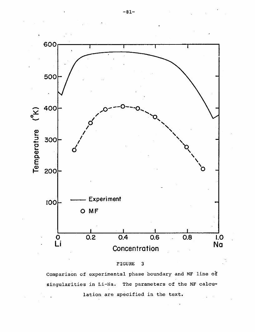
-81-

600

500

400- ,- .-.."

I I I

" 200 -o

100-- Experiment

OMF

0 0.2 0.4 0.6 0.8 1.0Li Concentration Na

FIGURE 3

Comparison of experimental phase boundary and MF line of

singularities in Li-Na. The parameters of the MF calcu-

lation are specified in the text.

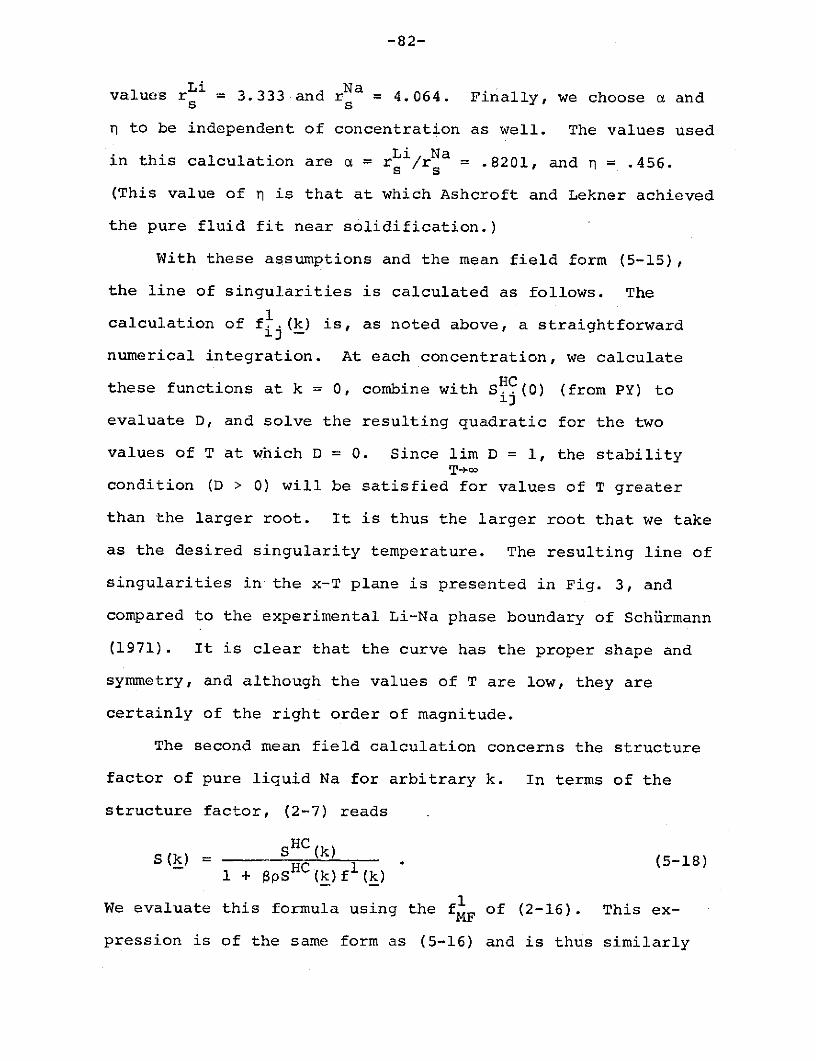
-82-

values rL = 3.333 and rN = 4.064. Finally, we choose a ands s

n to be independent of concentration as well. The values used

Li Nain this calculation are a = rs /r = .8201, and r = .456.

(This value of n is that at which Ashcroft and Lekner achieved

the pure fluid fit near solidification.)

With these assumptions and the mean field form (5-15),

the line of singularities is calculated as follows. The

calculation of f. (k) is, as noted above, a straightforward

numerical integration. At each concentration, we calculate

these functions at k = 0, combine with S HC (0) (from PY) toij

evaluate D, and solve the resulting quadratic for the two

values of T at which D = 0. Since lim D = 1, the stability

condition (D > 0) will be satisfied for values of T greater

than the larger root. It is thus the larger root that we take

as the desired singularity temperature. The resulting line of

singularities in the x-T plane is presented in Fig. 3, and

compared to the experimental Li-Na phase boundary of Schirmann

(1971). It is clear that the curve has the proper shape and

symmetry, and although the values of T are low, they are

certainly of the right order of magnitude.

The second mean field calculation concerns the structure

factor of pure liquid Na for arbitrary k. In terms of the

structure factor, (2-7) reads

HCS (k)S = (k) = . (5-18)1 + pS H C (k)fl (k)

We evaluate this formula using the fMF of (2-16). This ex-

pression is of the same form as (5-16) and is thus similarly

-83-

3.

2.0

1.0

0.00 2 4 6 8 10 12 14

y (= ka)

4a.HC

S. (y) in PY for n = .456.

1.00

.50

y (= ka)

2 48 10 12 14

-.25

4b.HC 1DMF(y) = 1 + pS (y) flF (y) for Na at T = 3710 K.

FIGURE 4

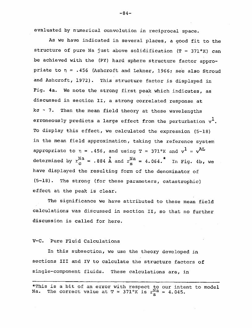
-84-

evaluated by numerical convolution in reciprocal space.

As we have indicated in several places, a good fit to the

structure of pure Na just above solidification (T = 371 0 K) can

be achieved with the (PY) hard sphere structure factor appro-

priate to n = .456 (Ashcroft and Lekner, 1966; see also Stroud

and Ashcroft, 1972). This structure factor is displayed in

Fig. 4a. We note the strong first peak which indicates, as

discussed in section II, a strong correlated response at

ka - 7. Then the mean field theory at these wavelengths

erroneously predicts a large effect from the perturbation vl

To display this effect, we calculated the expression (5-18)

in the mean field approximation, taking the reference system

appropriate to n = .456, and using T = 371 0 K and v = vAL

Nao Na *determined by r a = .884 A and r = 4.064. In Fig. 4b, we

have displayed the resulting form of the denominator of

(5-18). The strong (for these parameters, catastrophic)

effect at the peak is clear.

The significance we have attributed to these mean field

calculations was discussed in section II, so that no further

discussion is called for here.

V-C. Pure Fluid Calculations

In this subsection, we use the theory developed in

sections III and IV to calculate the structure factors of

single-component fluids. These calculations are, in

*This is a bit of an error with respect to our intent to modelNa. The correct value at T = 371 0 K is rNa = 4.045.s

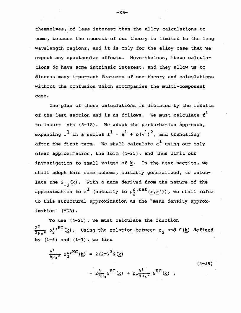
-85-

themselves, of less interest than the alloy calculations to

come, because the success of our theory is limited to the long

wavelength regions, and it is only for the alloy case that we

expect any spectacular effects. Nevertheless, these calcula-

tions do have some intrinsic interest, and they allow us to

discuss many important features of our theory and calculations

without the confusion which accompanies the multi-component

case.

The plan of these calculations is dictated by the results

of the last section and is as follows. We must calculate fl

to insert into (5-18). We adopt the perturbation approach,

expanding fl in a series f = a + o(v ) 2, and truncating

after the first term. We shall calculate a using our only

clear approximation, the form (4-25), and thus limit our

investigation to small values of k. In the next section, we

shall adopt this same scheme, suitably generalized, to calcu-

late the Sij (k). With a name derived from the nature of the

approximation to a1 (actually to ppref(r,r')), we shall refer

to this structural approximation as the "mean density approx-

imation" (MDA).

To use (4-25), we must calculate the function

a2 ,HCD2 , p 2 (k). Using the relation between p 2 and S(k) defined

by (1-6) and (1-7), we find

a2 .,HC 3ap 2 p2 (k) = 2(2r) 6(k)

(5-19)

+ 22 CS (k) + po~ 2 S (k)

-86-

At this point, we face a rather difficult matter. Of the two

parameters, p and a, needed to specify the HC reference sys-

tem, p is determined by the particular system under investi-

gation, while a is left to choice. We shall shortly have a

good deal to say on the subject of the best choice of a. The

important point for now is that if a is selected by any scheme

ALsystematically related to the potential v , it will depend on

the density through the rs dependence of this potential. A

question which might be asked is, should the density deriva-

tives in (5-19) properly include density derivatives of this

"best" a? This question is actually the first manifestation

to this point of what is ultimately a fundamental difficulty

in applying this work to metallic systems, where the notion of

an ion-ion pair potential depends crucially on the accounting

of conduction electron effects. We shall discuss this matter

in section V-F. For now, however, we proceed from the assump-

tion, stated in section I, that the ionic structure factors

are those appropriate to a classical fluid with pair inter-

actions v A L . Then once a potential vAL has been constructed,

and subsequently modelled by a hard core plus tail, we shall

investigate the appropriate classical structure without fur-

ther consideration of the origin of these potentials. Within

this view, if the parameter a is -accepted as a characteristic

ALof the potential v , it is a given in the problem, and the

differentiations in (5-19) are performed only with respect to

the explicit density dependence.

We can thus use the definition (5-9) of n to replace

-87-

Poo by n - " On making this change in (5-19), and substi-

tuting into (4-25), we find

a (k) = v1 (k)

(5-20)

+ dk' v 1 k'){- sHC(k-k + 2 SHC (k-k')}P (2r) ' a2 12

We note further that since p2 (r) = 0, identically for r < a,

we must also have ;po2 HC(r) = 0, identically, for r < a.

Then (remembering that (4-25) is just the Fourier transform of

(4-24)), we see that al(k) in this approximation is explicitly

independent of the form of v l ( r) for r < a. Thus, as dis-

cussed earlier, we make the replacement v = vAL. Finally,

making the first order approximation fl = a , we have, for the

mean density approximation to f ,

f (k) = v (k)

(5-21)

+ 1 dk' AL k) { SHC (k - k ' ) + 2 -2 SHC(k - k ' ) }

Po (2) 3 a - 2 an 2

We note that the n.derivatives of the structure factors can be

given an explicit analytic form in the PY approximation, so

that the expression in (5-21) is calculated by numerical

integration of analytic functions.

We first specialize this calculation to the case of the

absolute long wavelength limit, k = 0. Our interest in this

case derives from two sources. First, at k = 0, the expres-

sion (5-20) for a (0) is exact (for the hard core plus tail

potential). Then the only approximations we make in this case

-88-

are the first order approximation, and, of course, the PY

approximation for HC (k). Secondly, at k = 0, the physical

meaning of our results can be discussed using the well-known

compressibility sum rule:

lim S(k) = a- TN (5-22)

where the expression in braces is the isothermal compressi-

bility.

We have calculated S(0) in the MDA for the vA L appropri-

ate to four alkali metals, Li, Na, K, and Rb, at, in each

case, the temperature appropriate to melting. To specify each

metallic system, we need to specify rs, rc, and Z. The values

of rs listed in Table I are calculated for each element from

the density at melting (Smithells, 1967). The rc value for

Rb is taken from Al-II, while the other rc values are those

listed in Ashcroft and Langreth (1967C). The valence Z is

unity in each case. For the hard sphere reference system, we

follow the suggestion of Ashcroft and Lekner (1966) that each

of these elements at melting should be characterized by the

same packing fraction. We therefore take the reference fluid

in each case to be a hard sphere liquid of the appropriate

density with n = .456. Within the PY approximation, this

yields SHC(0) = .02396.

The results are presented in Table I. The first three

entries after each element are the melting temperature TM, rsat melting, and rc in A. The next column presents the values

calculated for fl(0) according to (5-21). We must say a word

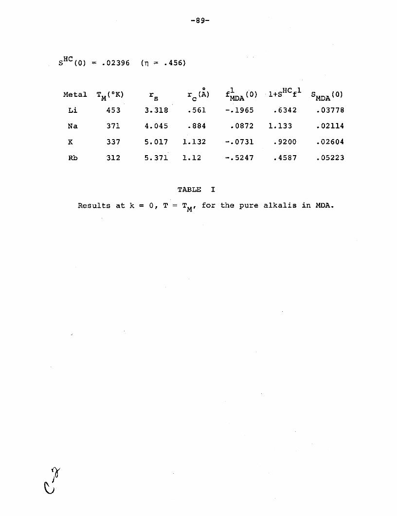
-89-

S HC(0) = .02396 (n = .456)

1 HC 1Metal T M(K) r r (A) 1+S f Sc fMDA 0 MDA 0

Li 453 3.318 .561 -.1965 .6342 .03778

Na 371 4.045 .884 .0872 1.133 .02114

K 337 5.017 1.132 -.0731 .9200 .02604

Rb 312 5.371 1.12 -.5247 .4587 .05223

TABLE I

Results at k = 0, T = TM, for the pure alkalis in MDA.

U

-90-

about the dimensions used for the entries in this column. In

1 1 ALthis, and all subsequent reportings of f , v , and v , we

adopt the convention of reporting not these figures directly,

but the dimensionless ratio between these figures and the

quantity 47Z 2 e 2 /(kTF )2 = ZEF/Po. (Here, kTF is the usual

Thomas-Fermi wavenumber, or, in the notation of (5-4), just

2kf 2 .) Thus, for example, in the column labelled fl(0), we

actually quote the values of, say, E(0), where

1 4r Z2 e 2f (0) = 2 (0). (5-23)

(kTF)2

In these terms, the important quantity pofl(k) is given by

23 ZE(k)TF/T, where TF is the usual Fermi temperature. The

last two columns present, from these values of fl, the values

of the denominator in (5-18) and the resulting S(0).

We note from the compressibility sum rule (5-22) and the

comparison between S(0) and SHC(0), that the compressibility

can be either increased or (in the case of Na) decreased by

the addition of vl. Numerically, this reflects the fact that

the calculated values of f (0) are of either sign. We note

that, for these potentials, the mean field form f 1(0) (whichMFc 1is, from (2-16), just fov (r)r2dr ) will not have this proper-

ty, since the potentials vl defined here are predominantly

negative for r > a. (These potentials are displayed in AL-II.

In relation to the hard sphere diameter defined by n = .456,

they each take a form qualitatively like that displayed in

Fig. 2.) That the correct from of fl(0) should in fact permit

either sign is apparent from the fact that these negative v1

-91-

nevertheless contain both attractive and repulsive regions.

At sufficiently high density, the nearest neighbor position

will be placed in the repulsive region of v1 , so that a de-

crease in compressibility is expected on passing from hard

core to hard core plus tail models. This is, of course, a

correlation effect, since a nearest neighbor position can only

be defined for correlated particles. It is instructive to

note, from AL-II, that the nearest neighbor position in Na is

indeed just into the repulsive part of vl, while in Rb, it is

well into the attractive region.

We turn now to the results at k 0. In Fig. 5, we

present the functions fl(k) for Li, Na, and K, calculated in

the MDA (that is, by (5-21)). Note that to present only

fl (k), we need not present the temperature (though temperature

will affect the careful selection of r s .) As with the k = 0

results, we plot these functions in units of 47Z 2e2/(kTF) 2 .

The MDA is a long wavelength (first order) approximation

for fl. We expect it to be valid for wavelengths longer than

the correlation range in the reference fluid. The correlation

range should be given roughly by the inverse of the width of

the first peak in SHC(k), since this peak defines the dominant

oscillation of the radial distribution function g(r) (see

equation (1-6)). From consideration of the HC structure

factor of Fig. 4a, we expect, optimistically, that what we

might call the range of "a priori validity" of the MDA should

extend only out to ko - 1. The interesting feature of the

results presented in Fig. 5 is that, in spite of strong

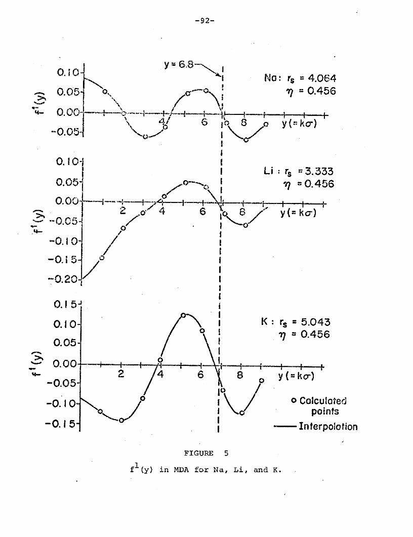
-92-

O. hI No: rs = 4.064

0.0 = 0.456

-0.054 L 0 6 8 y(= ko)0. 0-L0.05-0.10-i

I Li: rs = 3.333I0.05o = 0.456

S. 4 6 Iy (= ko-)0. 0 /

-0.10 I

-0. ; 15 -o

I-0.20J I

0.1 5

0.10 K: rs = 5.0430.05 = 0.456

0.05-

0.00 --2 4 6 8 y (= ko-)

-0.05 o

-0.1 ,, oo o Colculated

-0.15 - Interpolotion

FIGURE 5

fl (y) in MDA for Na, Li, and K.

-93-

variations in the shape and amplitude of the curves, the

curves all go through zero at a value of ko near the hard

sphere peak (kapeak = 6.8). This means that for a small

region around the peak, the MDA gives to S(k) values which are

in accord with our physical expectation that S(k) should be

little affected at the peak by vl. This region is really very

narrow. In Na, the structure factor has been driven to

negative values by ka = 7.0. (Note from (1-5) that the struc-

ture factor is a positive definite quantity.) Yet the exist-

ence of such a region in each element seems to suggest that

this effect may be, as discussed at the end of section IV, a

manifestation of finite particle size.

Until now, we have been content to neglect the problem of

selecting the hard sphere reference parameters in favor of

illustrating, with simple (but not unreasonable) values, the

general features of these theories. Though we shall adopt

this tactic once more to make a point when we turn to the bi-

nary alloy case, we must ultimately consider the selection

these parameters with care. It is convenient to begin the

discussion of this matter before we leave the simpler pure

fluid case.

For the pure fluid, we wish to develop a systematic pro-

cedure for selecting the "best" a of the model potential

(5-12), given the potential vAL . The aim of this work is to

be able, with this model, to calculate closely the structure

appropriate to vAL Consideration of the physics involved

-94-

suggests that, with a good enough perturbation theory, a could

be defined through an empirical approach. The work proceeds

in two stages. We first model the potential vAL with the po-

tential of (5-12), that is, with a potential which is infinite

for all r less than some diameter a, and equal to the real po-

tential for r > a. We then calculate the structure by a per-

turbation theory in which the perturbation is that part of VAL

which lies outside the core of diameter a. Consider for a

moment a sequence of such models for a single potential vA L

arranged in order of decreasing a. If we could sum all orders

of the perturbation series, and hence calculate exactly the

structure appropriate to each model potential, we should find

in this sequence that the structure eventually becomes inde-

pendent of a. This will happen when vA L takes on a value at

r = a which is more than a few kT above its minimum value.

Then further decreases in a will affect the model potential

only in a region which is virtually never sampled. In reality,

of course, we can calculate the structure only in an approx-

imation which is based fundamentally on the smallness of the

perturbation. With decreasing a, the perturbation becomes

larger, and the approximation will eventually break down. If,

however, the approximate theory works reasonably well for a

perturbation of order one or two times kT, we might observe

some vestige of the ideal result. That is, there might still

be a small range of a for which the calculated structure is

independent of a. This structure would clearly be the struc-

ture we are after.

-95-

To search for such a region, we repeated, for many values

of n, the S(0) calculation for pure liquid Na described above.

A region of independence does not appear. In fact, the result

is quite strongly dependent on n. At T = 371 0 K and for

Na 0 NarNa .884 A and r = 4.064, the values of S(o) in the MDAc s

vary almost linearly between .0335 at n = .400 and .0140 at

n = .500. The result of this calculation is plotted in

Fig. 6. This result provides a revealing and not too encour-

aging look at the adequacy of the approach.

In any case, this result means that the best we can do is

try to devise an external criterion for selecting a which will

bring the calculated model structure closest to the structure

ALappropriate to v . It is clear that the essence of that

criterion will be to select the largest hard sphere diameter

consistent with a reasonable modelling of the potential. This

consideration suggests an approach in the spirit of that taken

by Ashcroft and Langreth (AL-II), who selected a as that point

ALin the core region of v (r) at which the potential has risen

kT above its minimum. Such an approach seems to contain the

essential physics of our problem. In more recent work (e.g.

Stroud and Ashcroft, 1972) a diameter a was selected for a

different problem by a variational approach. This approach is

based on the result (Lukes and Jones, 1968)

F < FHC + <U> , (5-24)

where F is the free energy of the fluid with internal poten-

tial U(R), FHC is the free energy of some hard core fluid, and

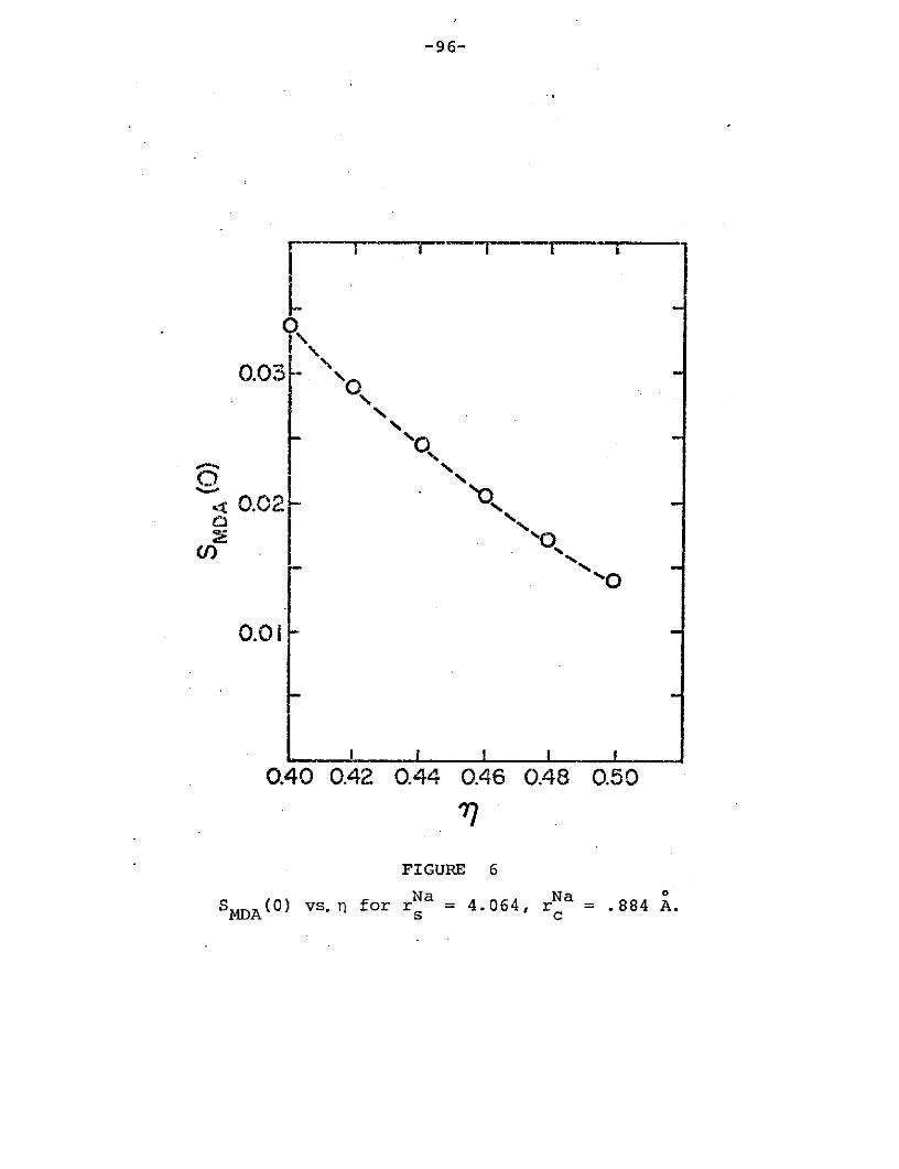
-96-

0.03 -O\

. 0.02 -

OE

0.01 -

0.40 0.42 0.44 0.46 0.48 0.50

FIGURE 6

Na Na oS MDA(0) vs.n for r = 4.064, r = .884 A.MDA

-97-

<U>HC is the thermal average of U(R) taken with the hard core

distribution functions. For the case of a pure fluid with

pair interaction v AL, (5-24) reads

F < FHC + dr dr' v AL (r - ' )poHC(r,r ' ) . (5-25)

In an effort to calculate the liquid free energy, the right

side of this inequality can be minimized with respect to the

hard core diameter a. Though such an approach may seem to

bear little direct relation to our problem, it, in fact,

3appears to contain essentially the same physics as the T kT

rule, for it gives very nearly the same results for both the

magnitude and temperature dependence of a. The advantage of

the variational approach is that the right side of (5-25) can

be simply expressed as an integral in reciprocal space and the

whole procedure automated to a great extent. We make use of

the generalization of this procedure for binary alloys in the

next section.

This completes the discussion of our results for pure

fluids.

V-D. Binary Alloys I: The k = 0 Results and Phase Separation.

In this subsection, we apply the theory of sections III

and IV to calculate for binary alloys the line of singulari-

ties in the x-T plane. The elements of these calculations are

the same as those of the mean field calculation presented in

V-B. We calculate fi and search for the highest temperature

at which D of (5-17) equals zero. In the present work,

-98-

however, we shall replace the mean field approximation to flij

by the mean density approximation, suitably generalized to the

alloy case. As in the case of the pure fluid calculations,

the MDA is exact in first order at k = 0, so that, once the

hard core plus tail potentials are specified, the only approx-

imations in the present section are the first order approxima-

tion and, as usual, the use of the PY approximation for theH C

S (k).ij -

To construct the MDA for the alloy case, we consider the

long wavelength approximation (4-31) to a. (k), and proceed as

we did for the pure fluid case. We can express the deriva-

tives HC(k) in terms of the S (k), the referenceap ap km ij

structure factors. We differentiate only the explicit density

1 ALdependence, make the replacement v.. = v. because the form of

13 ~3

(4-31) is observed to be independent of v. (r) for r < aij.j 1 1

and finally make the first order approximation f. = a. .. The1 3 13

result is a set of expressions for f1 (k) which are analogousij

to (5-21) but more complicated. These expressions are pre-

sented in appendix D. They form the MDA to fl.. We note that

for this case as well, the density derivatives may be given an

explicit form in the PY approximation, so that the calculation

1of aij, though by now a lengthy process, is in principle just

a numerical integration over analytic functions.

For the first calculation, we sought a comparison between

the mean field and mean density approximations. To do this,

we use the MDA in a calculation which is otherwise identical

to the mean field calculation of section V-B. That is, we set

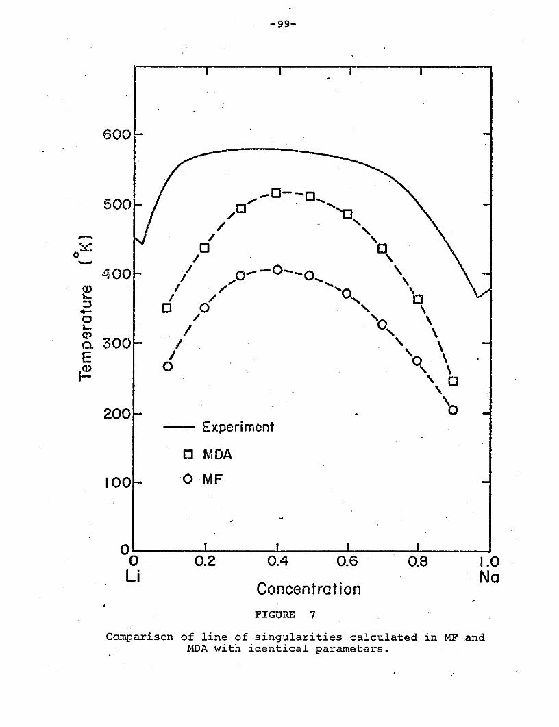
-99-

600-

500/ /- 00

t 0 0E / o

\ 0

200 0

I-

- Experiment

SM DA

100- 0 MF

o I I I

0 0.2 0.4 0.6 0.8 1.0Li NaLi Concentration No

FIGURE 7

Comparison of line of singularities calculated in MF andMDA with identical parameters.

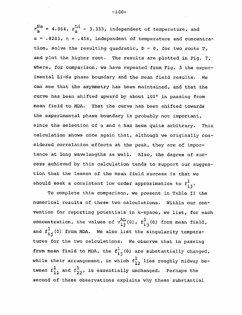
-100-

Na Lirs = 4.064, rs = 3.333, independent of temperature, and

a = .8201, n = .456, independent of temperature and concentra-

tion, solve the resulting quadratic, D = 0, for two roots T,

and plot the higher root. The results are plotted in Fig. 7,

where, for comparison, we have repeated from Fig. 3 the exper-

imental Li-Na phase boundary and the mean field results. We

can see that the asymmetry has been maintained, and that the

curve has been shifted upward by about 1000 in passing from

mean field to MDA. That the curve has been shifted towards

the experimental phase boundary is probably not important,

since the selection of a and n has been quite arbitrary. This

calculation shows once again that, although we originally con-

sidered correlation effects at the peak, they are of impor-

tance at long wavelengths as well. Also, the degree of suc-

cess achieved by this calculation tends to support our sugges-

tion that the lesson of the mean field success is that we

should seek a consistent low order approximation to f..

To complete this comparison, we present in Table II the

numerical results of these two calculations. Within our con-

vention for reporting potentials in k-space, we list, for each

AL 1concentration, the values of v. (0), fij (0) from mean field,

and f. (0) from MDA. We also list the singularity tempera-

tures for the two calculations. We observe that in passing

from mean field to MDA, the f (0) are substantially changed,

while their arrangement, in which fl2 lies roughly midway be-1 1

tween f and f1 is essentially unchanged. Perhaps the

second of these observations explains why these substantial

-101-

x vAL12 MF 1 2 fMDA 212 TMF (K) TMDA (K)

.000 1.223 -.1382.455 -.1271.841 -.133

.100 1.190 -.150 -.202 265 3492.385 -.136 -.0591.787 -.144 -.168

.200 1.156 -.161 -.204 351 4342.314 -.145 -.0281.736 -.155 -.160

.300 1.124 -.172 -.201 394 4902.256 -.153 .0051.691 -.165 -.152

.400 1.093 -.182 -.213 406 5142.201 -.162 .0331.648 -.175 -.145

.500 1.065 -.193 -.218 396 5112.151 -.170 .0551.609 -.185 -.141

.600 1.037 -.203 -.223 369 4862.104 -.178 .0711.571 -.195 -.138

.700 1.012 -.214 -.230 327 4362.059 -.186 .0811.536 -.204 -.138

.800 .987 -.224 -.236 272 3582.017 -.194 .0851.503 -.214 -.140

.900 .964 -.234 -.244 205 2431.978 -.202 .0851.472 -.223 -.143

1.000 .935 -.2441.941 -.2101.438 -.232

TABLE II

Comparison of MF and MDA calculations of f (0) in Li-Na.ij(0 nL-a

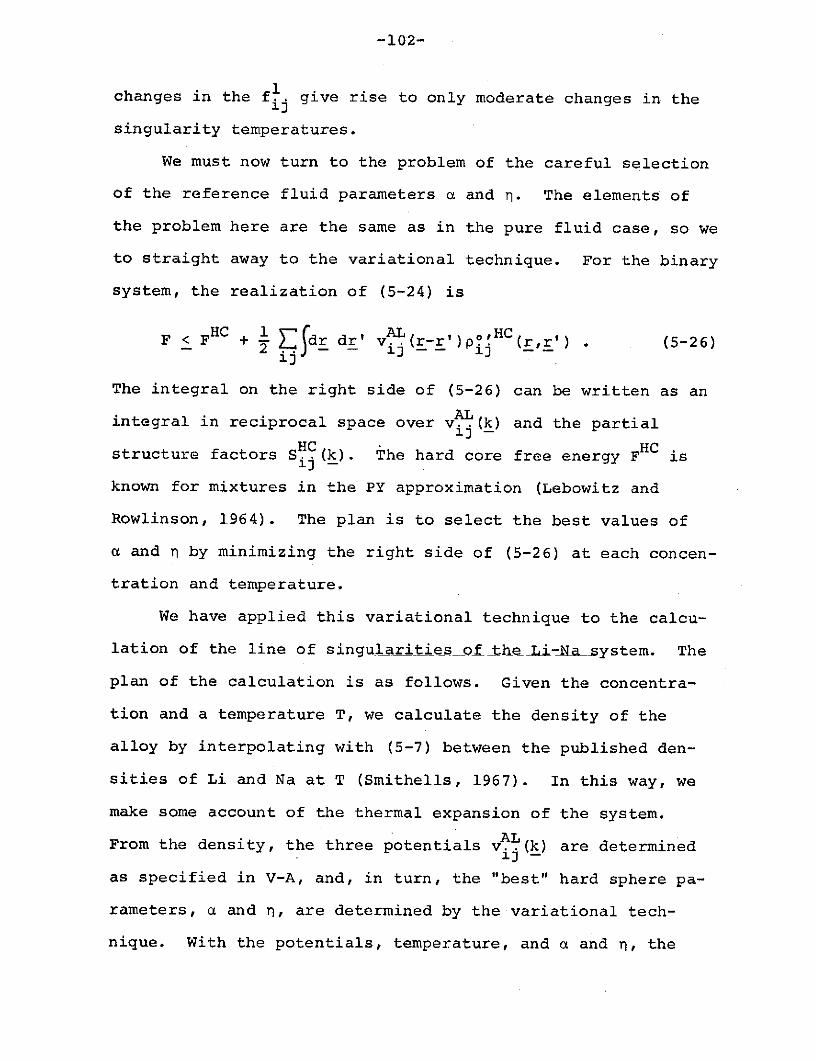
-102-

changes in the f give rise to only moderate changes in the

singularity temperatures.

We must now turn to the problem of the careful selection

of the reference fluid parameters a and n. The elements of

the problem here are the same as in the pure fluid case, so we

to straight away to the variational technique. For the binary

system, the realization of (5-24) is

H C 1 AL HCF < F + d dr' l (r- p (rr') . (5-26)2 iJ - - 13 - ij

The integral on the right side of (5-26) can be written as an

ALintegral in reciprocal space over vA.(k) and the partial

structure factors SH (k). The hard core free energy FH C isij

known for mixtures in the PY approximation (Lebowitz and

Rowlinson, 1964). The plan is to select the best values of

a and n by minimizing the right side of (5-26) at each concen-

tration and temperature.

We have applied this variational technique to the calcu-

lation of the line of singularities of the Li-Na system. The

plan of the calculation is as follows. Given the concentra-

tion and a temperature T, we calculate the density of the

alloy by interpolating with (5-7) between the published den-

sities of Li and Na at T (Smithells, 1967). In this way, we

make some account of the thermal expansion of the system.

ALFrom the density, the three potentials v.L (k) are determined

as specified in V-A, and, in turn, the "best" hard sphere pa-

rameters, a and n, are determined by the variational tech-

nique. With the potentials, temperature, and a and n, the

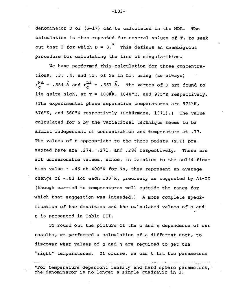
-103-

denominator D of (5-17) can be calculated in the MDA. The

calculation is then repeated for several values of T, to seek

out that T for which D = 0. This defines an unambiguous

procedure for calculating the line of singularities.

We have performed this calculation for three concentra-

tions, .3, .4, and .5, of Na in Li, using (as always)

Na o Li or = .884 A and r = .561 A. The zeroes of D are found toc c

lie quite high, at T = 1000'(, 10400 K, and 975 0K respectively.

(The experimental phase separation temperatures are 5740 K,

576 0K, and 560 0K respectively (Schirmann, 1971).) The value

calculated for a by the variational technique seems to be

almost independent of concentration and temperature at .77.

The values of n appropriate to the three points (x,T) pre-

sented here are .274, .271, and .284 respectively. These are

not unreasonable values, since, in relation to the solidifica-

tion value ~ .45 at 400 0K for Na, they represent an average

change of -.03 for each 100 0K, precisely as suggested by Al-II

(though carried to temperatures well outside the range for

which that suggestion was intended.) A more complete speci-

fication of the densities and the calculated values of a and

n is presented in Table III.

To round out the picture of the a and n dependence of our

results, we performed a calculation of a different sort, to

discover what values of a and n are required to get the

"right" temperatures. Of course, we can't fit two parameters

*For temperature dependent density and hard sphere parameters,the denominator is no longer a simple quadratic in T.

-104-

Li Nax T(OK) r r a T D(T)s s

.300 950 3.42 4.28 .770 .280 -.033

1000 3.42 4.30 .768 .274 .005

1050 3.44 4.32 .772 .266 .029

.400 573 3.34 4.12 .771 .351 -.608

773 3.38 4.20 .762 .315 -.233

900 3.40 4.25 .770 .292 -.095

1000 3.42 4.30 .773 .277 -.020

1040 4.43 4.32 .771 .271 .005

.500 950 3.42 4.28 .774 .288 -.015

975 3.42 4.29 .772 .284 .000

1050 3.44 4.32 .775 .274 .048

TABLE III

Results of the variational calculation for Li-Na. Values for

Li Nar and r are calculated from published density datas s

(Smithells, 1967), a and n are determined by the variational

technique, and D(T) (at k = 0) is calculated in the MDA. The

points presented were calculated in the search for T at which

D(T) = 0.

-105-

to a single data point, but, for each concentration, there

presumably exists a locus of points in the a-n plane for which

D = 0 at the desired temperature. Then the scheme of this

calculation is as follows. Given the concentration x (we

choose x = .4, near the critical value, so that the line of

singularities lies close to the phase boundary), the observed

phase separation temperature is defined (575 0K from Schiirmann,

1971). Then the density and three potentials are calculated

for this x and T as described above, and the value of D inves-

tigated as a function of a and n. In Fig. 8, we present the

a-n plane for T = 575 0 K and x = .4. The boundary in this

plane divides the region where D is greater than zero (above

the boundary) from the region where D is less than zero. The

boundary itself is then the desired locus of points at which

D = 0. For comparison, the variational values assigned to a

and n at this x and T are a = .772 and n = .35.

The range of what we might consider reasonable values for

a and n is determined primarily by our physical feeling for

the packing fraction n. We do not want to select n much above

~ .47, since the experience in pure fluids suggests that the

system would tend to crystallize. Since 575 0 K is about 1250

above the melting point of Li (at x = .4, the mixture is Li

rich), the experience of AL-II might suggest an n of .41 to

.42. (The lower value obtained from the variational calcula-

tion presumably reflects both the presence of Na and the

effects of thermal expansion.) For these reasons, we have

chosen to exhibit in Fig. 8 the region between n = .35 and

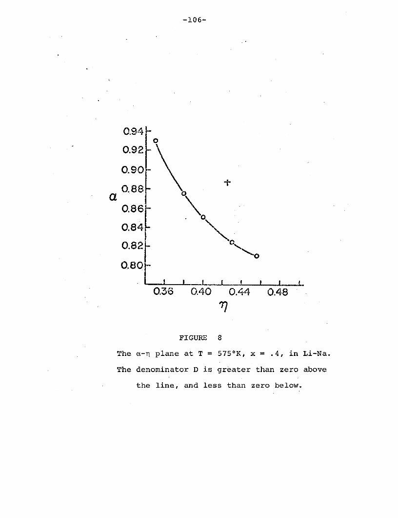
-106-

0.94-

0.92

0.90 -

0.84

0.82 -0.801-

0.36 0.40 0.44 0.48

FIGURE 8

The a-n plane at T = 575 0 K, x = .4, in Li-Na.

The denominator D is greater than zero above

the line, and less than zero below.

-107-

n = .46.

From these results, the selection of a and n emerges as

one of the central difficulties in our work. It is clear that

the temperature at which D = 0 is quite sensitive to the val-

ues of these parameters. The variational, calculation, which

probably has the best a priori justification, has yielded tem-

peratures which are far too high. We have seen that the

"correct" temperature can be obtained with "reasonable" values

for a and n but the physical meaning of those values, indeed

the physical meaning of such a fitting procedure, is unclear.

The confusion at this point suggests that, while we may ulti-

mately have learned something of the form of the structure

factors near phase separation, considerably more work on the

modelling of the systems (and on the theory itself) may be

needed before we can predict this transition in real systems.

Our difficulties here may also derive from the special problem

of the metallic pair potential, to which we shall turn briefly

in section V-F.

V-E. Binary Alloys II: The Results for Finite k.

We turn now to our results in the MDA for binary alloys

at finite k. In the previous section, we identified points at

which

lim D(k) = 0 , (5-27)k+0

where D(k) is the denominator of (5-17). In this section, we

examine one such point in detail, to discover the manner in

-108-

which D(k) goes to zero in the MDA as k-*0, and to observe the

MDA structure factors themselves. Ultimately, we intend such

work to form the basis of a resistivity calculation, and we

conclude this section by suggesting a program for such a

calculation.

We have chosen the point defined by x = .4, T = 575 0K,

a = .825, and n = .430. The values of a and n were estimated

from earlier results to give D(0) = 0 in Li-Na at this concen-

tration and temperature. These estimates are in fact slightly

in error, so that the value of D(0) is -.0013. In Table IV,

we list values of y = k/2kF and the corresponding values of

D(y) in the MDA. These values of y were selected in another

unit system, and turn out in the present units to be multiples

of .01692, a fact which we have indicated in the second column

of Table IV. In these units, the first peak of the structure

factor occurs at about y = 1.2, so that the region in which

the MDA is most to be trusted extends out to roughly y = .2.

When these values of D are plotted vs. y on a log-log plot,

they are observed to follow quite well a straight line of

slope two for the small values of y, but move away from this

line for the larger values (see Fig. 9). This suggests that

the singularity may be of the sort

D = a + bk 2 . (5-28)

This type of singularity appears in more conventional mean

field theories. Because of the error in a and n, we would ex-

pect for these data to set a = -.0013. This suggests that we

-109-

y(=k/ 2kF) y/.01692 D(y) D(y)-D(O)

0.00 0 -.0013 .0000

.03384 2 .0102 .0115

.05076 3 .0245 .0258

.06768 4 .0442 .0455

.08460 5 .0690 .0703

.10152 6 .0985 .0998

.11844 7 .1322 .1355

.13536 8 .1678 .1691

.16920 10 .2526 .2539

.20304 12 .3418 .3431

.25380 15 .4748 .4761

.33840 20 .6579 .6592

.50760 30 .7951 .7964

.67680 40 .8709 .8722

TABLE IV

Results in MDA for D(y) at y # 0. Calculated for Li-Na at

x = .4, T = 5750 K, a = .825, and n = .430.

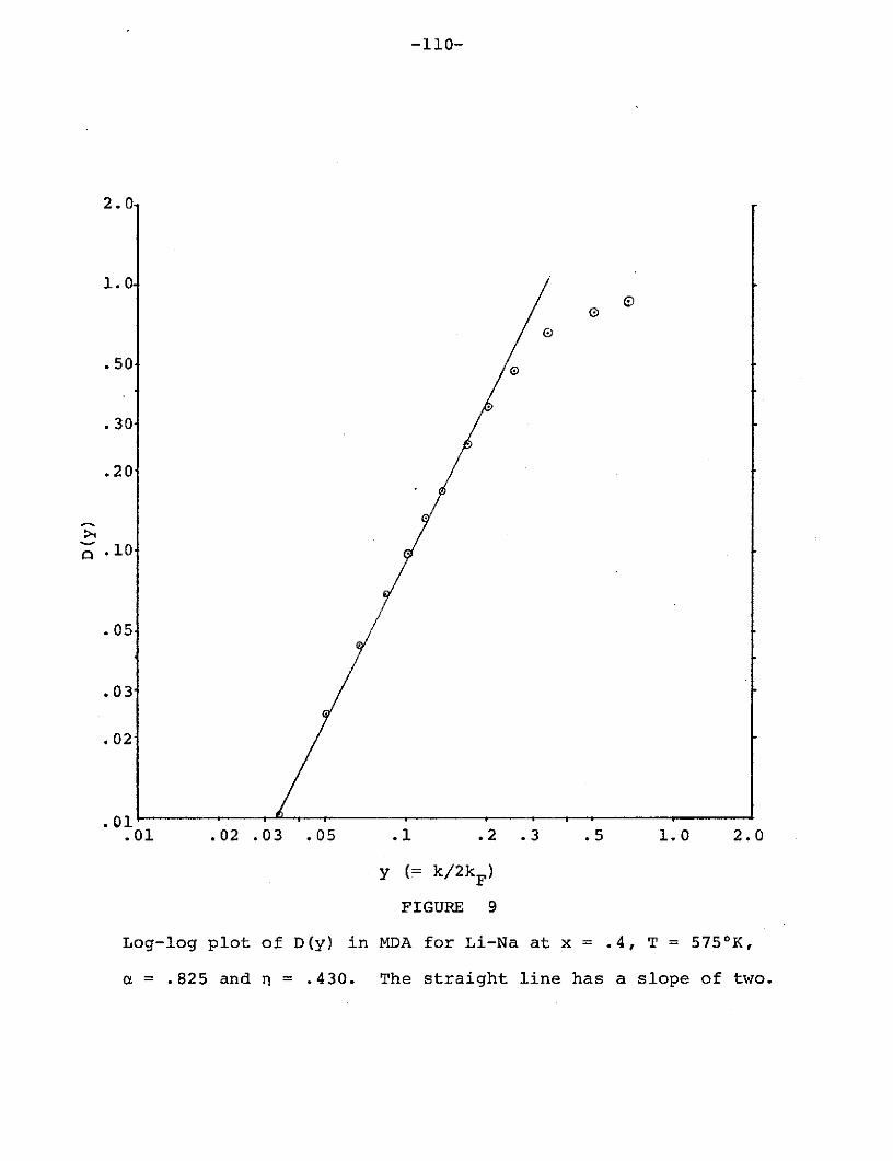
-110-

2.0

1.0

.50

.30

.20

.10o

.05

.03

.02

.01 .02 .03 .05 .1 .2 .3 .5 1.0 2.0

y (= k/2k F )

FIGURE 9

Log-log plot of D(y) in MDA for Li-Na at x = .4, T = 5750 K,

a = .825 and n = .430. The straight line has a slope of two.

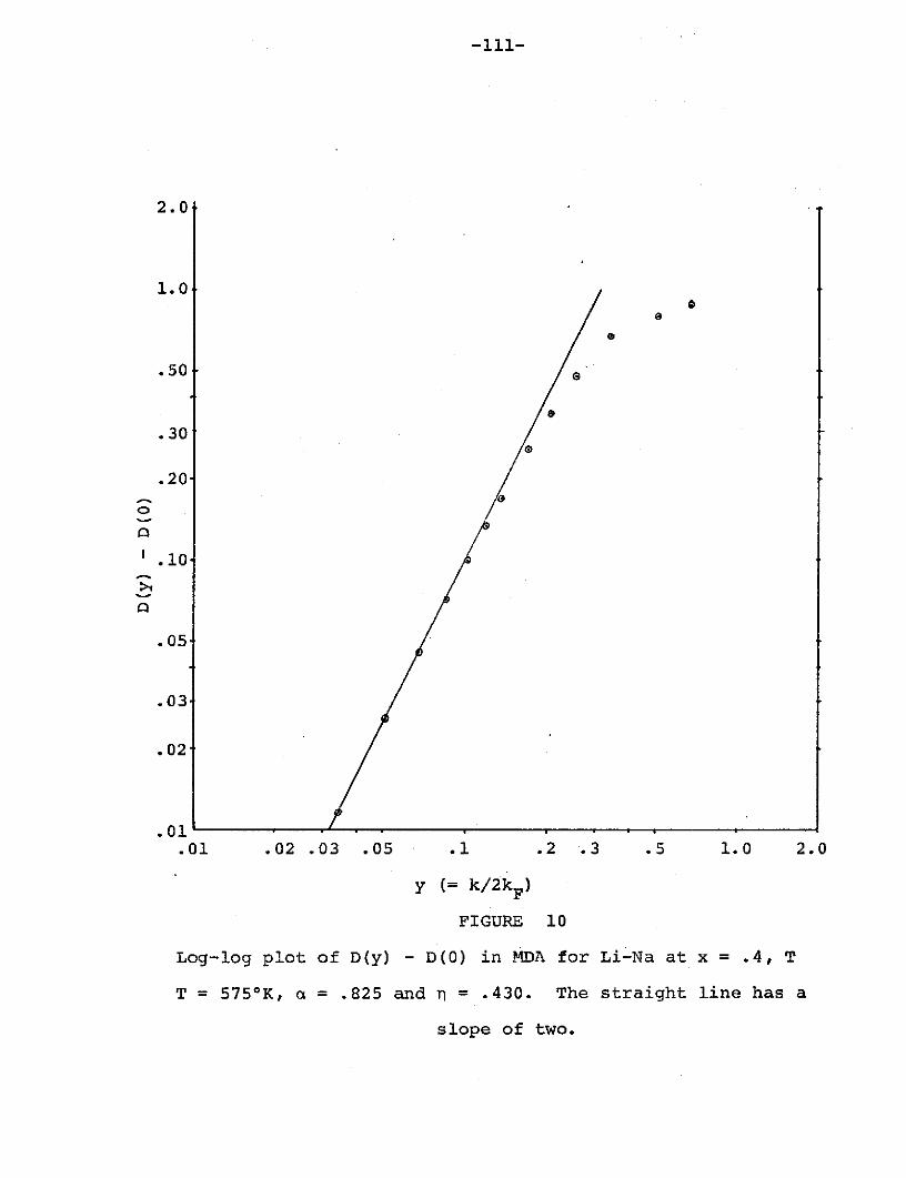
2.0

1.0

.50 o

.30

.20

S.10

.05

.03

.02

.01 ..

.01 .02 .03 .05 .1 .2 .3 .5 1.0 2.0

y (= k/ 2 kF)

FIGURE 10

Log-log plot of D(y) - D(0) in _MDA for Li-Na at x = .4, T

T = 575K, a = .825 and n = .430. The straight line has a

slope of two.

-112-

construct a log-log plot of (D + .0013) vs. y. This has been

done, and is presented in Fig. 10. The straight line in this

figure also has a slope of two, and now appears more properly

as an asymptote. This observation lends support to the pro-

posed form (5-28), viewed as a limit.

There are two points to be made about these results.

First, they coincide with the physical expectation that the

singularity at k = 0 is the first (highest temperature) of the

possible long wavelength singularities. This must be true on

physical grounds, since any singularity will render the system

unstable, while real alloy systems of critical concentration

are stable down to the critical temperature, at which point

the structure factors diverge at k = 0. Secondly, while we-2

can present no direct evidence for a k-2 singularity, we must

-4have a singularity which occurs less rapidly than k- 4 in order

that the resistivity integral (1-1) converge at the lower

limit. That our long wavelength approximation conforms to

both these physical expectations, despite the complexity of

the binary alloy formulas, is a gratifying result.

In Figure 11, we present the structure factors S. (k)13

calculated at this point in the MDA. They have been formed

using (3-40) for the Xij and the relation (3-5) between Xij

and S... In the same figure, we have presented for comparison13

the (PY) structure factors of the underlying hard core refer-

ence mixture (the mixture defined by x = .4, a = .825, and

n = .430). The MDA structure factors appear to join rather

smoothly with the HC structure factors at point roughly midway

-113-

5.0-

Si] (y) MDA

4.0

MDA

3.0 S2 2

2.0-

1.0 -/HC 2 /,S1 0* HC

0.5 1.0

-HC--12'- y(= k/2kF)- I.0

-2.0 /0

-3.0- MDA * MDA: calculated points

S 12 M DA: interpolation

S--- HC-4.0 -FIGURE 11

Partial structure factors for Li-Na at x = .4, T = 575 0 K,a = .825, and n = .430. The solid lines represent thestructure in the MDA, and the dashed lines represent thestructure of the hard sphere reference system.

-114-

between the origin and the first peaks. This fact is in ac-

cord with our physical expectation for these systems, and, as

discussed below, might be put to good use in a resistivity

calculation. However, the MDA is expected to be valid only

for small k (y < .2) so that the ultimate meaning of this ob-

servation is unclear.

This completes the report on the calculations we have

performed for metallic systems. Although we have stopped

short of a resistance calculation, we can at least indicate

the shape that such a calculation may take. We are interested

in shedding some light on the conjecture, discussed in section

I, that the resistivity anomaly observed by Schirmann and

Parks in Li-Na is a long wavelength effect. As indicated in

(1-1), what we need for a resistance calculation is the form

of the S.ij (k) for 0 < k < 2kF. What we have is an approxima-

tion valid for small k (0 < k S 2kF/ 7) and the physical idea

that the structure factors S..(k) should remain substantially13

unchanged around the peaks as we pass from hard core to hard

core plus tail model potentials. It is immediately clear that

we are in no position to do any serious quantitative calcula-

tion. Yet we might still imagine a calculation which could

lend qualitative support to the long wavelength hypothesis.

We might, for instance, simply calculate the contribution to

the resistivity from that part of the integral in (1-1) for

which the MDA is valid. More completely, we might calculate

the structure in the MDA at small wavelengths, and join the

results smoothly to the HC structure factors around the peaks,

thus incorporating what we expect will be the essential fea-

tures of S.. (k) near phase separation. (As noted above, the

MDA, somewhat inexplicably, seems to be doing this job for

us.)

The trick in any such calculation, of course, is going to

be to get the T-dependence right (since we are looking for a

temperature dependent effect.) This involves understanding

both the "normal" (that is, linear) and the anomalous parts of

the resistivity. We might, however, simplify a first calcula-

tion by supposing that the "normal" part is ultimately attrib-

utable to the hard cores, that is, could be dealt with by a HC

structural model of sufficiently subtle temperature dependence.

(In view of the successful resistivity calculations of AL-II,

this may not be an unreasonable assumption.) Under such an

assumption, the plan of a first simple calculation would be to

ignore the temperature dependence of the density and the

"best" hard sphere model, and study only the remaining T de-

MDA HCpendence of the difference pelec - Pelec" We plan to under-

take such a calculation in the near future.

V-F. The Metallic Pair Potential

In these calculations for metallic liquids, we have sev-

eral times encountered the conceptual difficulty arising from

the density dependence of the pair potential. We have also

encountered a great deal of difficulty in getting our calcu-

lated results to agree in more than general form with the ex-

perimental results for the real systems. It seems to us in

-116-

retrospect that these difficulties may be traceable to an in-

correct assumption made at the outset, namely, that the ionic

structure is precisely that appropriate to (classical) parti-

ALcles interacting via the pair potential v . We have not un-

dertaken a detailed and careful investigation of this problem.

Yet it seems to us that there is, within the tradition which

ALgave rise to the effective potential v , a certain contradic-

ALtion in usage which suggests that the potential v is incor-

rectly used to calculate the structure factors at small k.

Whether this is in fact the case is a difficult (and still

open) question.

The difficulty appears in the following way. Our calcu-

lations are based on an approximate accounting of energy in

simple metallic systems (Ashcroft and Langreth, 1967C, and

Harrison, 1966). For this discussion, the essential features

of this approximation are contained in the form

E(p,,R) = E 1 (PO) + E 2 (Po,R) . (5-29)

The terms belonging to E1 (po ) depend only on the average dens-

ity p, = N/V. The terms belonging to E2(po,R) depend on the

explicit ionic positions R as well as on p,. When E2 is cal-

culated within a linear screening approximation, the result

can be cast as a sum over an effective ion-ion pair potential.

With the choices of dielectric function and pseudopotential

specified in V-A, this potential becomes vAL.

Without going further into the origins and form of this

expression, we can make the important points here by consid-

-117-

ering and contrasting how it has been used in the calculation

of the compressibility and structure of simple metals. In

each of these calculations, we are considering the effects of

density variations. To calculate the compressibility, we con-

sider variations in the average density po. A calculation of

S(k), however it proceeds, must be equivalent to considering

spatially varying densities, since S(k) is the density linear

response function. Viewed in this way, the two calculations

differ only in that the appropriate density variations are of

infinite wavelength in the first, and of finite wavelength in

the second. Yet the customary use of (5-29) in these calcu-

lations requires a fundamental distinction between these two

cases, hence, between infinite and finite wavelength density

variations. Good values of the compressibility are obtained

if one considers all of the p, dependence in (5-29). On the

other hand, the structure factor is calculated ignoring E1 (Po )

entirely, and also ignoring the density dependence of E2 (Po,R),

ALthat is, of v . (Of course, p, = N/V is constant in the ca-

nonical ensemble. Our question will be, is this always the

correct density to use in calculating the energy?) This re-

duces the structural problem to the problem of a classical

liquid with pair interaction v AL, and, as discussed in I-D,

places the hard sphere success on a good foundation.

The point we wish to make is that, whatever its successes,

this procedure rests on too sharp a distinction between finite

and infinite wavelength. Indeed, for long wavelengths, the

distinction is blurred. This must be so because the correla-

-118-

tions (both ionic and electronic) in the liquid are of only

finite range. Then a density variation with a wavelength much

longer than the range of correlations must have effects which

are locally indistinguishable from those of a change in po

which gives the same local density. With this blurring of the

distinction between finite and infinite wavelengths comes an

ambiguity in the structure calculation at long wavelength. In

our calculations, we have followed the traditional method of

ALignoring the po dependence and treating v as a valid pair

potential at all finite wavelengths. Yet it seems from this

discussion as if, at long wavelengths, we must discover how to

ALinclude the effects of E1 (p.) and the po dependence of v ,

presumably by evaluating these somehow at the local density.

It is not clear which view (if either) is correct.

We remark that this discussion is confined to the consid-

eration of long wavelengths. With respect to these matters,

the existing short wavelength calculations seem to be less in

doubt. A density variation of wavelength much shorter that

the range of ionic or electronic correlations will look over

this range nothing at all like a change in p,. We expect the

existing pair potential approximation to be valid for such

wavelengths. These wavelengths will include the first peak in

S(k). Then, in particular, the success of the hard sphere

model, which means primarily the ability of this model to re-

produce the experimental first peak, is probably still attrib-

ALutable to the form of v .

Clearly, a careful and systematic investigation of this

-119-

matter is required before we can remove the ambiguity at long

wavelengths, and define a consistent procedure. We mention

that efforts are being made (Watabe and Hasegawa, 1972A,B) to

treat the structural and thermodynamic properties of pure

metallic liquids by considering these systems from the outset

as binary systems composed of ions and electrons. We suggest

here that one fruitful line of study for the particular prob-

lem at long wavelength (and in the present tradition) might be

to consider calculating the energy of the metal in a perturba-

tion theory that begins, not with the uniform electron gas,

but with the non-uniform electron gas studied by Hohenberg and

Kohn (1964) and Kohn and Sham (1965).

We note finally that if careful investigation of the long

wavelength problem proves our calculations to be wrong, they

may still be viewed as model calculations, which illustrate

the form of the structure factors near phase separation (and

thus may still give us a qualitative understanding of the

resistive anomaly). The developments of sections III and IV,

although carried out with metallic systems in mind, stand

quite independently of these systems within the tradition of

classical liquid theory.

VI. Discussion, Conclusions, and Suggestions for Further

Work

This work has been divided into two parts: the develop-

ment of the perturbation theory of the hard core plus tail

mixture, and the application to the metallic liquids and

alloys. Although some items to be discussed relate to results

from both parts, we shall adopt this same division in this

last section.

VI-A. The Perturbation Theory

We have cast our study of structure in terms of the func-

tions fij(k), which we may take as defined by (3-33). These

functions are closely related to the more familiar direct cor-

relation functions of Ornstein and Zernike (1914) (see equa-

tion (3-35)). Perhaps our most important result for these

functions is the equation (3-75), which shows that to calcu-

late these functions to first order in the perturbing poten-

tials v., we must calculate p ref(r,r'), the two body func-

tion in the non-uniform reference fluid, to second order in

6pi(r). This observation leads directly to the long wave-

length approximation (4-31). As indicated at the close of

section IV, a successful approximation for short wavelengths

may possibly be developed by a carefully chosen analogy to

crystalline solids.

In this effort, we have produced a theory which retains

many of the virtues of the "simplest" mean field theory of the

-120-

-121-

phase transition itself (that is, the theory defined by (4-9)

and used by Stroud (1973) in his study of phase separation),

but which is, in principle at least, a reasonable theory of

structure (which the simplest mean field theory is not.) It

incorporates, in principle, the hard sphere successes, and is

in the spirit of the most successful of the present theories

of simple liquids, the perturbation theories on a HC reference

system.

We note here that, while our effort has concentrated on

the structure factors, we have actually been doing thermo-

dynamic perturbation theory as well. To make this point, we

consider the form of the Zwanzig expansion of the free energy

F (in the absence of external fields.) Writing

U(R) = Ur e f + Ul(R), where U (R) is defined by (3-68), spe-

cializing to pure fluids, and introducing an expansion param-

eter X by replacing vl by Xv , we find quickly (from (3-1)

with (R) = 0)

aF S<1 (R)> V- dr vl (r)p (r) , (6-1)<U (R)> = 2 2

where < > and po'(r) are evaluated from the distribution

function determined by U(R) = Uref(R) + XU (R). Then

a2 F X vA V2 jdr v1(r) - po- (r) . (6-2)

DX2 2 ax 2

Using (6-1) and (6-2) in a A expansion of FA about A = 0 and

setting A = 1, and writing p.=0(r) ( = ,ref (r)) in terms2

-122-

of S (k) by (1-6) and (1-7), we find eventually

r dkF ref + N o {v (0) + dk 1 ref(

2 Po (27) -Np{ 1 - 1 ref 2

S- k v (k) (S (k)) (-8poa (k))} (6-3)4 Po) (2) 3 -

+ o(vl)

.where al (as defined in (3-73)) is the first order term in the

X expansion of fl. That is, the second order term in the

ref 1Zwanzig expansion of (2-2) may be calculated knowing S , v ,

and aI . At the present level of our work, of course, in which

we have only a long wavelength approximation to al(k), we are

not yet able to perform a sensible approximate calculation of

this second order term in F. Perhaps with better approxima-

tionsto p p,ref this situation will change. We note that this

second order term is, of course, the term studied by Barker

and Henderson (1967A, 1967B). In this sense, our MDA appears

similar in spirit (though not identical) to the "macroscopic

compressibility" and "local compressibility" approximations

introduced (and later abandoned) by these authors (1967A,

1972).

To proceed beyond the lowest order term in f , we note

again that fl is a well-defined, if inaccessible, sum in the

conventional perturbation series. Perhaps further progress

can be made by combining our view of fl with the perturbation

series approach. As a simple (and possibly important)

-123-

example, we know from the perturbation series for a pure fluid

that, whever a single term 8vl(r) appears, we can perform a

partial summation of higher order terms by replacing that

8v (r) with {l-e-$v'(r)}. (See, for example, Brout, 1965, or

Andersen and Chandler, 1972.) Then we may use (3-75) to gen-

erate a further approximation to fl specified by*

dr' -vl (-') p,ref (r,r') ref (r- d' e p (rr)P - (rr )

8 2 2

(6-4)

= dr dr' 6p(r)6p(r') f (r-r') + o(6p)

(The generalization to multi-component systems is presumably

straightforward.) The approximation represented by (6-4) must

represent a valid summation in the perturbation series, and

goes beyond any we have used in this work. Such an approxima-

tion will clearly affect the T-dependence of the results.

(Since, for the metallic systems, we have v1 explicitly only

in reciprocal space, the generalization of (3-75) to (6-4)

introduces non-trivial computational problems.) Direct exten-

sion of our approach to higher order seems all but out of the

question, since the expansion leading to (3-75) involves, in

the next term, the three and four body distribution functions

of the non-uniform fluid.

Now consider the adequacy of the overall approach, that

is, of the approach which calculates the structure by

*The constant term in {l-e - v i (r)} vanishes from (6-4) by thesum rule on- p2. (See Appendix A, equation (A-8)).

-124-

calculating fl in first order. We note that, in view of the

objection raised in the discussion of the metallic potentials,

our metallic calculations may not have provided a test of the

theory. It may be that the only test we have run on this

theory is the calculation of S MDA(0) for Na parameters and

several values of q. While the results of this test were not

encouraging, it is clearly incomplete and insufficient to

stand as the only test of the adequacy of the theory. More

complete and careful testing of this theory on model poten-

tials is clearly called for.

Application of this work to Lennard-Jones fluids will

require a little care, since the work finds its most natural

expression in reciprocal space. We will thus not be able to

use the full potential as the perturbation on the hard core as

we could for metals. Since, however, these results are expli-

citly independent of the form of vl(r) for r < a, we are at

liberty to give to vI a form inside the core which makes

Fourier transform of v1 possible. This is the approach taken

by Chandler et al. (1972) in their "optimized" RPA. Direct

application of this work to molecular liquids must be held

pending an understanding of the importance of the assumption

vl(r) = v1 (-r), which has apparently been required in several

places. The essentials of the approach, however, that is, the

view which takes the densities rather than the potentials as

the basic variables, may, in suitably generalized form, have

wide application in the theory of both simple and molecular

(insulating) liquids.

-125-

VI-B. Application to Metallic Liquids

We have used the results of sections III and IV to define

a long wavelength structural approximation which we have

called the mean density approximation (MDA). In application

to potentials modelled for the pure alkali metals, this ap-

proximation yields, at k = 0, results consistent with our

expectations for the compressibility. At values of k around

the reference (HC) peak, the results in the MDA seem to give

some indication of a finite particle size effect. At k = 0 in

the binary case, a simple model calculation of the line of

singularities reproduces quite well the asymmetry and position

of the Li-Na phase boundary in the x-T plane. Because the

correct line of "hypothetical" singularities lies below the

phase boundary at all points but the critical point, we expect

qualitatively the more rounded shape we observe in the calcu-

lated curve. The selection of the hard sphere reference pa-

rameters emerges as a central problem. This problem, however,

was studied almost entirely with respect to metallic poten-

tials and real systems, so that, in view of the difficulty

with the metallic potential, we clearly need to do more work

in the spirit of the test at S(0), that is, in the spirit of

calculations for model systems. The nature of the singularity

as k-0 was investigated, and appears asymptotically to be of

the form (a + bk2)-l (a gratifying result in view of the com-

plexity of the MDA formulas), a form which insures the conver-

gence of the resistivity integral (1-1) at the lower limit.

The partial structure factors in the MDA were calculated and

-126-

plotted vs. k for one combination of parameters.- Suggestions

were made for a simple resistivity calculation which might

shed some light on the nature and origin of the anomaly ob-

served by Schirmann and Parks. Finally, a possible difficulty

of the metallic potential at long wavelength was noted and

suggestions made for work on the problem.

These calculations tend to support the hypothesis that

the separation transition is driven primarily by the tail of

the potential. This suggests that the study of such phase

transitions could ultimately yield useful experimental infor-

mation on this long range part of the potential. Such infor-

mation has been difficult to extract from the structure fac-

tors themselves, since these tend to be dominated by the geo-

metric effects of the repulsive cores. It is obvious, how-

ever, that an enormous amount of theoretical progress is still

required. A certain amount of pessimism may be justified.

A question which remains unanswered is why some metallic

binaries separate and others do not. One need only consider

Na-K, rather than Li-Na, to find a binary system in which the

uniform phase is stable at all concentrations for any temper-

ature above solidification. Our physical understanding of

this matter is that phase separation (a long wavelength order-

ing) and freezing (a short wavelength ordering) must in each

system be competing transitions. A calculation of sufficient

subtlety should show that, in Li-Na, the separation transition

occurs at a higher T than a (hypothetical) freezing transi-

tion, while the converse is true in Na-K. It remains to be

-127-

seen whether such a calculation can be performed successfully

with present techniques.

The theory of the phase transition implicit in the MDA

is, of course, essentially mean field, so that we do not ex-

pect this work to shed any light on the usual problems encoun-

tered in the study of critical exponents (Fisher, 1964). The

critical exponents in this problem are defined by Schirmann

(1971), to whose work the interested reader is referred. We

have paid little attention to this view of the problem and its

necessary introduction of Ising type models, in favor of an

approach directly through the structural results and calcula-

tions of classical liquid theory.

The structural work has been presented with a resistivity

calculation ultimately in view. The work, of course, will

have application near the phase transition to other properties

of liquid metals which depend on the structure (e.g. the

thermopower, thermal conductivity, optical absorption, ultra-

sonic absorption). Before such problems can be studied with

any confidence, however, it seems that we must resolve the

difficulty of the pair potential approximation at long

wavelength.

Appendix A: The Distribution Functions

We shall define the distribution functions for a pure

fluid. The generalization to mixtures is straightforward but

cumbersome. We consider a system of N particles in a volume V

at temperature T, and evaluate thermal averages in a canonical

ensemble. We define the N particle distribution function

PN(R) = e -$U(R) e - (R)/(fdR e -SU(R) e - S(R)) (A-l)

(just as in (3-9)). This function satisfies

JdR PN (R) = 1 . (A-2)

In terms of this function, the thermal average of some quan-

tity A(R) is calculated, just as in (3-63), by

<A(R)> = $dR A(R) PN(R) . (A-3)

The n-body distribution function is defined by

Pn (rl',r2'" .. rn)(A-4)

N! fdrn+ ... dr P (rl,r2,...r ;r ,...r(N-n)! +l drN PN1 N'-' nn+l' rN)

For n = 1,

p (r) = Ndr 2 ... dr PN (r,r 2 ,...r) , (A-5)

is just the single particle density. This function clearly

satisfies the sum rule

Idr Pl(r) = N . (A-6)

-128-

-129-

For n = 2,

P2 (r,r') = N(N-l) dr 3 dr 4 ... dr N PN(r,r',r 3 , ... N ) (A-7)

is the two body distribution function which plays the impor-

tant role in our work. It has the meaning that p2 (r,r')dr dr'

is the probability of finding a particle in dr about r and

another in dr' about r'. It satisfies the sum rule

Tdr dr' p2 (r,r') = N(N-1) . (A-8)

Now consider the role of these functions in a thermal

average, using (A-3). First consider the thermal average of

the sum on single particle potentials ((R) defined, as in

(3-2) , by

N(R) = (r.) . (A-9)

i=1

Then

< =(R)> = dr dr ...dr *(r.) PN(rl,...r) . (A-10)

Because PN is a symmetric function of its arguments, we may

make in each integral in (A-10) the change of variables r.ir ,

and r 1 r.. Since all N integrals are then seen to be equiv-

alent, we have

< =(R)> NJdrl 4(r 1) dr 2 .... dE N PNrr22,...) . (A-11)

By (A-5), this is just

<(R)> = dr p(r)pl(r) . (A-12)

-130-

Next calculate the thermal average of the sum of pair

potentials U(R) defined, as in (3-42), by

U(R) 1= v(r.-r.) . (A-13)2 . -1

Then

<U(R)>= __drd ... dr v(r.-r.) P (r ... ). (A-14)2 2-3 N 1 rN

We use the symmetry of PN(R) to make, in each integral of

.(A-14), the changes of variable ri+rl' r lr., r.jr2 , and

Er2r.. Then all N(N-1) integrals in (A-14) are seen to be2 -3

equivalent, and we have

<U(R)>(A-15)

= - N(N-1) drldr 2 v(r -r 2 ) dr 3 . ..dr PN(,r12 1 -2 3 ... -N N -2 N

so that, by (A-7), we find

<U(R)> = lJdr dr' v(r-r')p (r,r') . (A-16)

Finally, consider the thermal average of the density

operator 8(k) defined by (1-3). In real space, this operator

is

(r) = (r-r . (A-17)

Then

<(r)> = drldr ... dr 6(r-r.) P (r,...) . (A-18)Using the symmetry of PN(R),N we make, in each integral of

Using the symmetry of P (R), we make, in each integral of

-131-

(A-18), the changes of variable rir and rl-r., so that all

N integrals in (A-18) are seen to be equivalent, and we have

<(r)> = Ndr 6(r-r) dr 2 ...dr PN(rl,r 2 ,...r )

(A-19)

= Pl(r) ,

by (A-5). Then (r) is, as stated in section I, the operator

whose thermal average is the single particle density. Similar

arguments will establish the relations, given in (1-6) and

(1-7), between S(k) defined in terms of O(k) (in (1-2)) and

the two body distribution function p2 (r,r').

Appendix B: Phase Separation and Singularities in the Sij(k).

Here we wish to elaborate on the conclusions stated in

section I concerning the relation between phase separation and

singularities in the partial structure factors Sij(k) in the

limit as k+O.

The analysis concerns the form of the Gibbs energy per

particle, g(x), plotted as a function of x at constant T and

p. For some T1 < TC , this isotherm will have a form like that

presented schematically in Figure B-1. This curve exhibits

regions where it is concave upward and regions where it is

concave downward. In the region where the curve is concave

downward, between the points labelled C and D, we have

(a2(x) < 0 , (B-l)kax2 T,p

so that the system is unstable against concentration fluctua-

tions. The points A and B are defined (uniquely) by construc-

ting a line tangent to this curve at two points. A straight-

forward calculation of the Gibbs energies involved (bearing in

mind particle number conservation) shows that, for any concen-

tration between xA and xB (say XE), the Gibbs energy of the

uniformly mixed phase is higher than that of some separated

phase, and that the separated phase with the lowest Gibbs

energy is that defined by xA and xB. On the other hand, for

concentrations outside this region, x < xA or x > xB, the

Gibbs energy of the uniform phase is lower than that of any

separated phase. Then the concentrations xA and xB mark the

-132-

-133-

I-I

I I.I A_

0.0 XA XE XB 1.0

Concentration

FIGURE B-1

Gibbs energy per particle as a function of concen-

tration at T = T 1 < TC .

-134-

points in the x-T plane at which the line T = T1 intersects

the phase boundary. (Refer to the discussion in section I-A.)

As the temperature is raised, these points move closer togeth-

er, until, at the critical temperature TC, they coincide. For

all T > TC , the curve is everywhere concave upward. Then a

common tangent may not be constructed, and the uniform alloy

is stable in all concentrations.

Our concern is with the inflection points C and D, at

which

(a2g(X) 0 . (B-2)T,p

Bhatia and Thornton (1970) have shown that these are the

points at which the partial structure factors of the uniform

alloy diverge in the limit as k+0. It is clear that, at the

temperature T1 represented by the isotherm in Figure B-l,

these points are.not accessible. They must lie below the

phase boundary in the x-T plane. As the temperature is in-

creased towards TC, however, these inflection points will move

closer together until, at TC , the inflection points and the

common tangent points coincide. It is thus only at the criti-

cal point that the singularity is fully realized at separation.

Then the line of singularities in the x-T plane lies below the

phase boundary in general, but joins it at the one point which

is the critical point.

Appendix C: The k = 0 result (4-32).

We note from (1-2) and (1-3) that

S..(0) = (N.N.) <N i.N.> - (NiNj.) .. (C-1)

We evaluate <N.N.> in a grand canonical ensemble at constant13

T, V, and chemical potentials pi. Consider the pure fluid

case, for which

EN I!e N dR e - OU(R)

<N> = (C-2)E1 eSNdR e - S U(R)

N

Then we find

( IT<N> = B(<N 2 > - <N> 2) . (C-3)

Then

1 1 i <N> = <N2 > - <N> = S(0) (C-4)8 <N> TVN <N>T,V

That is

1 p <N>S(0) w- , where p = (C-5)

H T ,V

In a multi-component system, this result generalizes readily

to

S..ij(0) - (j (C-6)i j T,V,'

where the prime indicates that all p's are held fixed except

-135-

-136-

the one explicitly appearing in the derivative. By (3-5),

this result is

xij(0) lp -I, (C-7)\ j T,Vn'

Now, if pi is considered a function of all the p's, and pi is

considered a function of all the p's, we have

dP = ,V, ; d = dp , (C-8)I Pj T,V,p T,V,p

which gives

dpi = z. TV, T, Vdpy . (C-9)

This yields

-ap.1=6i P (C-10)j T,V,p' 9 T,V,p' '

or

P = U-1 (C-11)

where P is the matrix whose elements are (api/8j.) ,, andi J T,V, j

U is the matrix whose elements are (asj/ P)T,V,p'. Intro-

ducing the matrices X and F from (3-33), we then have, from

(C-7) and (C-ll),

X = -P = -U - 1 =-F - , (C-12)

so that F = U, or

fi (o) = (jT,, (C-13)

-137-

From thermodynamics, this is

i.0) P) (C-14)fij (0) piPj T,V,p' (C-14)

where F now denotes the free energy of the system. To arrive

at (4-32), we expand f.. and F in powers of the perturbation

v . We introduce an expansion parameter X by replacing v1

with Xv , and expand fij as in section III:

fi (0) = fref(0) + Xa (0) + o() 2 (C-15)iJ ij ij

For the expansion of F, we simply insert the Zwanzig expan-

sion, which, as we saw in the argument to (3-75), is just

F = Fref + X<U 1 (R)> + o() 2 . (C-16)o,ref

On writing <U (R)> in terms of p?!ref (r,r'), just as in,,ref 1

(3-71), and substituting into (C-14), the desired result,

(4-32), follows immediately.

We note that this result is also (plausibly) consistent

with a certain limiting case studied by Lebowitz and Penrose

(1966). These authors replace v (r) with the form

v (r) = 3 (Ar) , (C-17)

and study the form of the free energy in the thermodynamic

limit and in the limit as X*0. In this limit, the potential

v becomes very weak and very long range. The limiting result

for the free energy is

F(p) = Fref(p) + 2 , (C-18)

-138-

where F(p) now denotes the free energy per unit volume, and

= fdr W(r) = dr 134(Xr) , for all X. (C-19)

This result is made plausible by consideration of (C-16),

which reads, for this choice of v

F(p ref dr 1 3(Xr)p ,ref(r) + o() 2 . (C-20)

(Note that between (C-16) and (C-20), both F and X have been

redefined.) If the dimensions of the system are much greater

than the range of X34(Xr), we can change variables in the

integral to write

F(p) = Fref(p) + -dr (r)pref(r/) + o() 2 . (C-21)

If we now take the thermodynamic limit and the-limit as X0O

(in that order, so that the dimensions of the system are

always much greater than the range of X 34(Xr)), we see that

the region of integration in which p0,ref(r/) differs from(r/) differs from

p2 ill shrink to zero. Then (C-18) will follow if, as seems

reasonable for this weak form of v (r), the higher order terms

may be neglected.

The result (C-18) yields, through (C-14), the mean field

result

f (0) = o = dr v1 (r) .(C-22)

This result can be obtained directly from (4-32) by a similar

plausibility argument. For this potential, (4-32) reads

-139-

fl (0) = dr v (r) pref(r) + o (v) 22 - ap2 2

(C-23)

2 a 2 ref 2=-dr (r) a-p- 2 r o )

where, for the last step, we again require that the dimensions

of the system be much larger than the range of X34(Xr). If we

perform the same limiting steps described above, the region

1 a2 .refwhere p 2 P2 re f (r/X) differs from unity is seen to shrink

to zero, so that (C-22) follows from the neglect of higher

order terms.

Appendix D: The MDA to f (k) for a Two-component Fluid.ij

Let x, = p1/p and x 2 = p2/p, where pl and p2 are the den-

sities of species one and two respectively, and p = p + p.

Define the partial packing fractions n] and r2 by ni=pfai3/6,

where a. is the hard core diameter associated with the ith

species. Then the MDA for f for a binary alloy isij

1 AL1 (11 12f f(k_) =7vii (k)

1 dk_ AL 2 a2 HC 1 HC+ )3 V (k') { n2 S 1 2(k-k') + S 12 (k-k')}

(x 1dk' AL 3 C i HC

+n SH (k-k')}3ni 12

x ' AL n 2 2

x 12 v 22 (k ' ) 2S 2 (k-k')

(D-l)

1 ALf2 (k) = V (k)12 12

1 AL (k ') { 2 2 HC (2 SHC(k-k')

X2p (27)3 3 1 2 anzn2 +1 2 11

+ 1 dk AL a2 HC 1 HC+ - v (k') {nIn2 S ( k - k ' ) + - S (k-k')3 12 3nDn2 12 4 12

2 aI 12 2 an2 12

1 .__ AL { L 2 HC HC+ -fk v 2( k') {l2 2 SHC(k - k ' ) + - SHC(k - k ' ) }

xp (2Tr) 3 22 2 an 1an2 22 2 2 an 22

-140-

-141-

1 1The form of f22 (k) may be obtained from the form of fll (k) by22 11replacing all subscripts '1' with subscripts '2', and vice

versa.

The ni derivatives of the Sij may be given explicit forms

in the PY approximation. If these forms are to be derived

from the published expressions (AL-II), care must be taken

that the right variables are held constant as the differen-

tiations are performed. The structure function S.. is a func-

tion of k, PI' P2' ol and 02. We stipulate, just as in the

pure fluid case, that the ai are held fixed. Then, for ex-

ample, some of the necessary derivatives in (4-31) take the

form

-. 0(D-2)pl k,p~ ,p ,02

The following discussion of the variables will be valid as

well for the more complicated derivatives derived from (4-31),

but we shall take the expression (D-2) as the simplest example.

From the definition of the ni, it is clear that we may

trade the five variables above for k, nl, n2, al, and G2 . We

then have

/(as..\ Ias..PlI k,po 1 , 2 1 2' 1'2

Further, since S.. is unchanged when we scale all lengths by13

the same amount, we have

S ij(k,nlV2,aol,02) = S ij (-lk,ld no2' o l2) , (D-4)

so that Sij.. may be considered a function of only the four

-142-

variables kal, ka2,' i t and n2. Then the expression (D-3)

becomes

l Ikkc 2 , 2 (D-5)(S-.

1 )kol,k2,' 2

If we now trade kao and ko2 for a - 01/0 2 and ko2 , we arrive

finally at the result

(aS..1 as..p k, :1 k2,a ) (D-6)

2 1k,p2,l,2 2 "2,' n2where Sij is now considered a function of ko2, a, 11, and n2.

Then the form quoted in AL-I must be rewritten, since the var-

iables in AL-I are ka2, a, x, and n.

REFERENCES

Alder, B. and Wainwright, T., 1958, Nuovo Cimento Suppl. 9,116.

Alder, B.J., 1964, J. Chem. Phys. 40, 2724.

Alder, B. J. and Hoover, W. G., 1968, in Physics of SimpleLiquids, H. N. V. Temperly, J. S. Rowlinson, G. S.Rushbrooke, editors, North Holland Publishing Co.Amsterdam.

Andersen, H. C., Weeks, J. D., and Chandler, D., 1971, Phys.Rev. A4, 1597.

Andersen, H. C. and Chandler, D., 1972, J. Chem. Phys. 57,1918.

Ashcroft, N. W., 1966, Phys. Letters 23, 48.

Ashcroft, N. W. and Lekner, J., 1966, Phys. Rev. 145, 83.

Ashcroft, N. W. and Langreth, D. C., 1967A (AL-I), Phys. Rev.156, 685.

Ashcroft, N. W. and Langreth, D. C., 1967B (AL-II), Phys. Rev.159, 500.

Ashcroft, N. W. and Langreth, D. C., 1967C, Phys. Rev. 155,682.

Ballentine, L. E., 1967, Phys. Rev. 158, 670.

Barker, J. A. and Henderson, D., 1967A, J. Chem. Phys. 47,2856.

Barker, J. A. and Henderson, D., 1967B, J. Chem. Phys. 47,4714.

Barker, J. A. and Henderson, D., 1972, Ann. Rev. Phys. Chem.23, 439.

Bhatia, A. B. and Thornton, D. E., 1970, Phys. Rev. B2, 3004.

Brout, R., 1965, Phase Transitions, W. A. Benjamin, Inc.,

New York, Amsterdam.

Chandler, D., Andersen, H. C., and Weeks, J. D., 1972, J.Chem. Phys. 56, 3812.

-143-

-144-

Cohen, M. L. and Heine, V., 1970, Sol. St. Phys. 24, 37.

Coopersmith, M. and Brout, R., 1963, Phys. Rev. 130, 2539.

Fisher, M. E., 1964, J. Math. Phys. 5, 944.

Fisher, M. E. and Langer, J. S., 1968, Phys. Rev. Letters 20,665.

Harrison, W. A., 1966, Pseudopotentials in the Theory ofMetals, W. A. Benjamin Inc., New York.

Hohenberg, P. and Kohn, W., 1964, Phys. Rev. 136, B864.

Hoover, W. G. and Ree, F. H., 1968, J. Chem. Phys. 49, 3609.

Kohn, W. and Sham, L. J., 1965, Phys. Rev. 140, A1133.

Lebowitz, J. L., 1964, Phys. Rev. 133, A895.

Lebowitz, J. L. and Rowlinson, J. S., 1964, J. Chem. Phys.,41, 133.

Lebowitz, J. L. and Penrose, 0., 1966, J. Math. Phys. 7, 98.

Lukes, T. and Jones, T., 1968, J. Phys. Al, 29.

Mermin, N. D., 1965, Phys. Rev. 137, A1441.

Ornstein, L. S. and Zernike, F., 1914, Proc. Acad. Sci.Amsterdam 17, 793.

Percus, J. K. and Yevick, G. J., 1958, Phys. Rev. 110, 1.

Rotenberg, A., 1965, J. Chem. Phys. 43, 4377.

Rowlinson, J. S., 1968, in Physics of Simple Liquids, (seeAlder and Wainwright, 1968.)

Rushbrooke, G. S., 1968, in Physics of Simple Liquids, (seeAlder and Wainwright, 1968.)

Schirmann, H. K., 1971, Ph.D. Thesis, University of Rochester.

Schirmann, H. K. and Parks, R. D., 1971, Phys. Rev. Letters27, 1790.

Singwi, K. S., Tosi, M. P., and Land, R. H., 1968, Phys. Rev.176, 589.

Singwi, K. S., Sj6lander, A., Tosi, M. P., and Land, R. H.,1970, Phys. Rev. BI, 1044.

-145-

Smith, E. B. and Alder, B. J., 1959, J. Chem. Phys. 30, 1190.

Smithells, C. J., 1967, Metals Reference Book, Fourth Edition,London, Butterwirths.

Stroud, D. and Ashcroft, N. W., 1972, Phys. Rev. B5, 371.

Stroud, D., 1973, Phys Rev. B8, 1308.

Thiele, E., 1963, J. Chem. Phys. 39, 474.

Watabe, M. and Hasegawa, M., 1972A, "Theory of Density Fluc-tuations in Liquid Metals," in The Properties of LiquidMetals: Proceedings of the Second International Confer-ence Held at Tokoyo, Japan, Sept., 1972, Sakae Takeuchi,Editor, Taylor and Francis LTD, London, 1973.

Watabe, M. and Hasegawa, M., 1972B, "Electron Theory of theThermodynamic Properties of Liquid Metals," in Propertiesof Liquid Metals (see Watabe and Hasegawa, 1972A.)

Wertheim, M. S., 1963, Phys. Rev. Letters 10, 32

Wood, W. W., 1968, in Physics of Simple Liquids (see Alder andWainwright, 1968.)

Ziman, J. M., 1961, Phil. Mag. 6, 1013.

Ziman, J. M., and Faber, T. E., 1965, Phil. Mag. 11, 153.

Zwanzig, R. W., 1954, J. Chem. Phys., 22, 1420.