Embed Size (px)
Citation preview
Materializing Knowledge Bases via Trigger GraphsEfthymia Tsamoura
Samsung AI Research
Cambridge, United Kingdom
David Carral
LIRMM, Inria, University of Montpellier, CNRS
Montpellier, France
Enrico Malizia
University of Bologna
Bologna, Italy
Jacopo Urbani
Vrije Universiteit Amsterdam
Amsterdam, The Netherlands
ABSTRACTThe chase is a well-established family of algorithms used to ma-
terialize Knowledge Bases (KBs) for tasks like query answering
under dependencies or data cleaning. A general problem of chase
algorithms is that they might perform redundant computations. To
counter this problem, we introduce the notion of Trigger Graphs(TGs), which guide the execution of the rules avoiding redundant
computations. We present the results of an extensive theoretical
and empirical study that seeks to answer when and how TGs can
be computed and what are the benefits of TGs when applied over
real-world KBs. Our results include introducing algorithms that
compute (minimal) TGs. We implemented our approach in a new
engine, called GLog, and our experiments show that it can be sig-
nificantly more efficient than the chase enabling us to materialize
Knowledge Graphs with 17B facts in less than 40 min using a single
machine with commodity hardware.
PVLDB Reference Format:Efthymia Tsamoura, David Carral, Enrico Malizia, and Jacopo Urbani.
Materializing Knowledge Bases via Trigger Graphs. PVLDB, 14(6):
XXX-XXX, 2021.
doi:10.14778/3447689.3447699
PVLDB Artifact Availability:The source code, data, and/or other artifacts have been made available at
https://github.com/karmaresearch/glog.
1 INTRODUCTIONMotivation. Knowledge Bases (KBs) are becoming increasingly
important with many industrial key players investing on this tech-
nology. For example, Knowledge Graphs (KGs) [29] have emerged
as the main vehicle for representing factual knowledge on the Web,
and enjoy a widespread adoption [44]. Moreover, several key in-
dustrial players, like Google and Microsoft, are building KGs to
support their core business. For instance, the KG developed at Mi-
crosoft is used to support question answering, while Google uses
KGs to enable various products to respond more appropriately to
This work is licensed under the Creative Commons BY-NC-ND 4.0 International
License. Visit https://creativecommons.org/licenses/by-nc-nd/4.0/ to view a copy of
this license. For any use beyond those covered by this license, obtain permission by
emailing [email protected]. Copyright is held by the owner/author(s). Publication rights
licensed to the VLDB Endowment.
Proceedings of the VLDB Endowment, Vol. 14, No. 6 ISSN 2150-8097.
doi:10.14778/3447689.3447699
user requests. The use of KGs in such scenarios is not restricted
only to database-like analytics or query answering: KBs play also a
central role in neural-symbolic systems for efficient learning and
explainable AI [21, 33].
A KB can be viewed as a classical database B with factual knowl-
edge and a set of logical rules P , called the program of the KB,
allowing the derivation of additional knowledge. One class of rules
that is of particular interest both to academia and to industry is
Datalog [1]. Datalog is a recursive language with declarative seman-
tics that allows users to succinctly write recursive graph queries.
Beyond expressing graph queries, e.g., graph reachability, Datalog
allows richer fixed-point graph analytics via aggregate functions.
LogicBlox and LinkedIn use Datalog to develop high-performance
applications, or to compute analytics over its KG [2, 42]. Google
developed their own Datalog engine called Yedalog [19]. Other
industrial users include Facebook, BP [9], and Samsung [36].
Materializing a KB (P ,B) is the process of deriving all the factsthat logically follow when reasoning over the database B using
the rules in P . Materialization is a core operation in KB manage-
ment. An obvious use is that of caching the derived knowledge.
A second use is that of goal-driven query answering, i.e., derivingthe knowledge specific to a given query only, using database tech-niques such as magic sets and subsumptive tabling [7, 8, 12, 51].
The last application is particularly useful in the presence of com-
putational or memory restrictions. Beyond knowledge exploration,
other applications of materialization are data wrangling [32], en-
tity resolution [34], data exchange [24] and query answering over
OWL [40] and RDFS [15] ontologies. Finally, materialization has
been also used in probabilistic KBs [53].
Problem. The increasing sizes of modern KBs [44], and the fact that
materialization is not a one-off operation when used for goal-driven
query answering, urge the need for improving the performance of
materialization. The chase, which was introduced in 1979 by Maier
et al. [38], has been the most popular materialization technique and
has been adopted by several commercial and open source engines
such as VLog [55], RDFox [43], and Vadalog [9].
To improve the performance of materialization, different ap-
proaches have focused on different inefficiency aspects. One ap-
proach is to reduce the number of facts added to the KB. This is the
take of some of the chase variants proposed by the database and
AI communities [10, 22, 45]. A second approach is to parallelize
the computation. For example, RDFox proposes a parallelization
technique for Datalog rules [43], while WebPIE [56] and Inferray

[49] propose parallelization techniques for fixed RDFS rules. Or-
thogonal to those approaches are those employing compression and
columnar storage layouts to reduce memory consumption [31, 55].
In this paper, we focus on a different aspect: that of avoiding
redundant computations. Redundant computations is a problem that
concerns all chase variants and has multiple causes. A first cause
is the derivation of facts that either have been derived in previous
rounds, or are logically redundant, i.e., they can be ignored without
compromising query answering. The above issue has been partially
addressed in Datalog with the well-known seminaïve evaluation
(SNE) [1]. SNE restricts the execution of the rules over at least
one new fact. However, it cannot block the derivation of the same
or logically redundant facts by different rules. A second cause of
redundant computations relates to the execution of the rules: when
executing a rule, the chase may consider facts that cannot lead to
any derivations.
Our approach. To reduce the amount of redundant computations,
we introduce the notion of Trigger Graphs (TGs). A TG is an acyclic
directed graph that captures all the operations that should be per-
formed to materialize a KB (P ,B). Each node in a TG is associated
with a rule from P and with a set of facts, while the edges specify
the facts over which we execute each rule.
Intuitively, a TG can be viewed as a blueprint for reasoning over
the KB. As such, we can use it to “guide” a reasoning procedure
without resorting to an exhaustive execution of the rules, as it is
done with the chase. In particular, our approach consists of travers-
ing the TG, executing each rule r associated with a node v over the
union of the facts associated with the parent nodes ofv and storing
the derived facts “inside” v . After the traversal is complete, then
the materialization of the KB is simply the union of the facts in all
the nodes.
TG-guided materialization addresses at the same time all causesof inefficiencies described above. In particular, TGs block the deriva-
tion of the same or logically redundant facts that cannot be blocked
by SNE. This is achieved by effectively partitioning the facts cur-
rently in the KB into smaller sub-instances. This partitioning also
enables us to reduce the cost of executing the rules.
Furthermore, in specific cases, TGs allow us to reason either
by completely avoiding certain steps involved in the execution of
the rules, or by performing those steps at the end and collectively
for all the rules. Our experiments show that we get good runtime
improvements with both alternatives.
Contributions. We propose techniques for computing instance-
independent and instance-dependent TGs. The former TGs are
computed exclusively based on the rules of the KB and allow us
to reason over any possible instance of the KB making them par-
ticularly useful when the database changes frequently. In contrast,
instance-dependent TGs are computed based both on the rules and
the data of the KB and, thus, support reasoning over the given KB
only. We show that not every program admits a finite instance-
independent TG. We define a special class, called FTG, including allprograms that admit a finite instance-independent TG and explore
its relationship with other known classes.
As a second contribution, we propose algorithms to compute
and minimize (instance-independent) TGs for linear programs: a
class of programs relevant in practice.
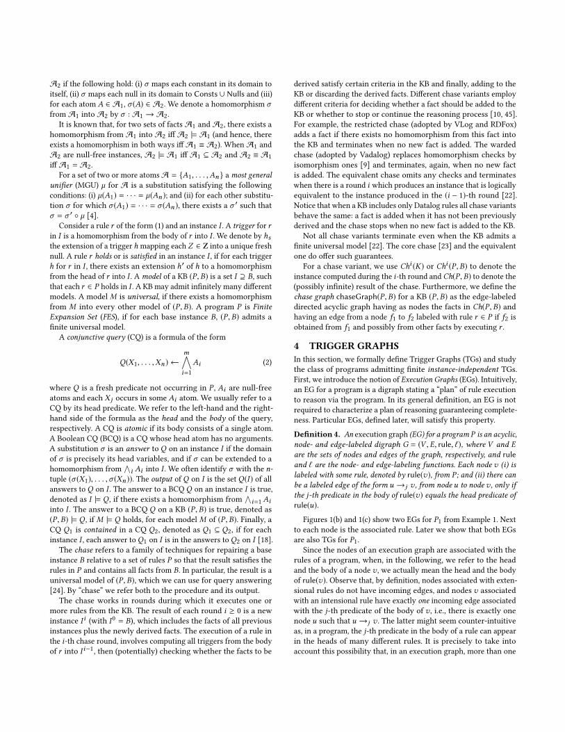
First roundInput Second round Third round
T (c2, c1, c2)
T (c2, c1, n1)
r(c1, c2)
R(c1, c2)
T (c2, c1, c2)
T (c2, c1, n1)
r(c1, c2)
R(c1, c2)
T (c2, c1, n1)
r(c1, c2)
R(c1, c2)
r(c1, c2)r1
r4 r2
r2 r3 r1 r3 r4 r1 r2 r3
r4
T (c2, c1, n1)
R(c1, c2) T (c2, c1, c2)
R(c1, c2) T (c2, c1, c2)
(a)
(b) (c)
u1 (created by r1)
u2 (created by r4)
u3 (created by r2)
u1 (created by r1) u3 (created by r2)
Figure 1: (a) Chase execution for Example 1, (b) the TG G1,(c) the TGG2. In (b) and (c), the facts shown inside the nodesare the results of reasoning over B using the TG.
A program P not admitting a finite instance-independent TG may
still admit a finite instance-dependent TG. As a third contribution,
we show that all programs that admit a finite universal model
also admit a finite instance-dependent TG. We use this finding to
propose a TG-guided materialization technique that supports anysuch program (not necessarily in FTG). The technique works byinterleaving the reasoning process with the computation of the TG,
and it reduces the number of redundant computations via query
containment and via a novel TG-based rule execution strategy.
We implemented our approach in a new reasoner, called GLog,
and compared its performance versus multiple state-of-the-art
chase and RDFS engines including RDFox, VLog, WebPIE [56] and
Inferray [49], using well-established benchmarks, e.g., ChaseBench
[10]. Our evaluation shows that GLog outperforms all its competi-
tors in all benchmarks. Moreover, in our largest experiment, GLog
was able to materialize a KB with 17B facts in 37 minutes on com-
modity hardware.
Summary. We make the following contributions:
• We propose a new reasoning technique based on travers-
ing acyclic graphs, called Trigger Graphs (TGs), to tackle
multiple sources of inefficiency of the chase;
• We study the class of programs admitting finite instance-
independent TGs and its relationship with other classes;
• We propose new techniques to compute minimal instance-
independent TGs for linear programs, and techniques to
compute minimal instance-dependent TGs for Datalog;
• We introduce a new reasoner, GLog, which has competitive
performance, often superior to the state-of-the-art, and has
good scalability.
A version of this paper with more details and proofs is in [52].
2 MOTIVATING EXAMPLEWe start our discussion with a simple example to describe how the
chase works, its inefficiencies, and how they can be overcome with
TGs. For the moment, we give only an intuitive description of some
key concepts to aid the understanding of the main ideas. In the
following sections, we will provide a formal description.
The chase works in rounds during which it executes the rules
over the facts that are currently in the KB. In most chase variants,
the execution of a rule involves three steps: retrieving all the facts
that instantiate the premise of the rule, then, checking whether the

facts to be derived logically hold in the KB and finally, adding them
to the KB if they do.
Example 1. Consider the KB comprising the databaseB = {r (c1, c2)}and the program P1 = {r1, r2, r3, r4}:
r (X ,Y ) → R(X ,Y ) (r1)
R(X ,Y ) → T (Y ,X ,Y ) (r2)
T (Y ,X ,Y ) → R(X ,Y ) (r3)
r (X ,Y ) → ∃Z .T (Y ,X ,Z ) (r4)
Figure 1 (a) depicts the rounds of the chase with such an input. In thefirst round, the only rules that can derive facts are r1 and r4. Ruler1 derives the fact R(c1, c2), which is added to the KB by the chase.Let us now focus on r4. Notice that variable Z in r4 does not occur inthe premise of r4. The chase deals with such variables by introducingfresh null (values). Nulls can be seen as “placeholders” for objects thatare not known. In our case, r4 derives the fact T (c2, c1, n1), where n1is a null, and the chase adds it to the KB.
The chase then continues to the second round where rules areexecuted over B′ = B ∪ {R(c1, c2),T (c2, c1, n1)}. The execution ofr2 derives the fact T (c2, c1, c2), which is added to the KB, yieldingB′′ = B′ ∪ {T (c2, c1, c2)}. Finally, the chase proceeds to the thirdround where only rule r3 derives R(c1, c2) from B′′. However, sincethis fact is already in B′′, the chase stops.
The above steps expose two inefficiencies of the chase. The
first inefficiency is that of paying the cost of deriving the same or
logically redundant facts.
Example 2. Let us return back to Example 1. The chase pays thecost of executing r3 despite that the execution of r3 always derivesfacts derived in previous rounds. Notice that this phenomenon is dueto the cyclic dependency between rules r2 and r3: r2 derives T -factsby flipping the arguments of the R-facts, while r3 derives R-facts byflipping the arguments of theT -facts. Despite that the SNE effectivelyblocks the execution of r1 and r2 in the third chase round, it cannotblock the execution of r3 in the third chase round, since T (c2, c1, c2)was derived in the second round.
Now, consider the factT (c2, c1, n1). This fact is logically redundantbecause it provides no extra information over the fact T (c2, c1, c2),which is derived by r2. Despite being logically redundant, the chasepays the cost of deriving it.
The second inefficiency that is exposed is that of suboptimally
executing the rules themselves: when computing the facts instanti-
ating the premise of a rule, the chase considers all facts in the KB
even the ones that cannot instantiate the premise of the rule.
Example 3. Continuing with Example 1, consider the executionof r3 in the second round of the chase. No fact derived by r4 caninstantiate the premise of r3, since the premise of r3 requires the firstand the third arguments of the T -facts to be the same. Despite thatthe premise of r3 cannot be instantiated using the derivations of r4,the chase unnecessary pays the cost of executing r3 over those facts.
The root of these inefficiencies is that the chase considers in each
round the entire KB as a source of potential derivations relying
only to the SNE for avoiding redundant derivations. If we were able
to “guide” the execution of the rules in a more clever way, then we
could avoid the inefficiencies stated above.
For instance, consider an alternative execution strategy where r2is executed only over the derivations of r1, while r3 and r4 are notexecuted at all. This strategy would not face any of the inefficiencies
highlighted above. Figure 1 (c) shows a graph for defining such
a strategy. Informally, a Trigger Graph (TG) is precisely such a
graph-based blueprint to compute the materialization.
In the remaining, we first provide a formal definition of TGs and
study their properties. Next, we show that under certain cases we
can compute TGs that support reasoning over any possible database
and present techniques for computing such TGs in a static fashion,
i.e., prior to reasoning. Next, we present techniques for computing
TGs at reasoning time and show that such TGs support a wider class
of rules than the ones statically computed. For both types of TGs
we provide techniques for eliminating redundant computations.
3 PRELIMINARIESLet Consts, Nulls, Vars, and Preds be mutually disjoint, (countably
infinite) sets of constants, nulls, variables, and predicates, respec-tively. Each predicate p is associated with a non-negative integer
arity(p) ≥ 0, called the arity of p. Let EDP and IDP be disjoint sub-
sets of Preds of intensional and extensional predicates, respectively.A term is a constant, a null, or a variable. A term is ground if it is
either a constant or a null. An atom A has the form p(t1, . . . , tn ),where p is an n-ary predicate, and t1, . . . , tn are terms. An atom Ais extensional (resp., intensional), if the predicate of A is in EDP(resp., IDP). A fact is an atom of ground terms. A base fact is anatom of constants whose predicate is extensional. An instance I isa set of facts (possibly comprising null terms). A base instance B is
a set of base facts.
A rule is a first-order formula of the form
∀X∀Y∧n
i=1Pi (Xi ,Yi ) → ∃Z.P(Y,Z), (1)
where, P is an intensional predicate and for all 1 ≤ i ≤ n, Xi ⊆ Xand Y ⊆ Y (Xi and Yi might be empty). We assume w.l.o.g. that the
premise of a rule includes only extensional predicates or intensional
predicates. We will denote extensional predicates with lowercase
letters and intensional predicates with uppercase letters. Universal
quantifiers are commonly omitted. The left-hand and the right-
hand side of a rule r are its body and head, respectively, and are
denoted by body(r ) and head(r ). A rule is Datalog if it has no
existentially quantified variables, extensional if body(r ) includesonly extensional atoms, and linear if it has a single atom in its body.
A program is a set of rules. A knowledge base (KB) is a pair (P ,B)with P a program and B a base instance.
Symbol |= denotes logical entailment, where sets of atoms and
rules are viewed as first-order theories. Symbol ≡ denotes logical
equivalence, i.e., logical entailment in both directions.
A term mapping σ is a (possibly partial) mapping from terms to
terms; wewriteσ = {t1 7→ s1, . . . , tn 7→ sn } to denote thatσ (ti ) = sifor 1 ≤ i ≤ n. Let α be a term, an atom, a conjunction of atoms, or a
set of atoms. Then σ (α) is obtained by replacing each occurrence of
a term t in α that also occurs in the domain of σ with σ (t) (i.e., terms
outside the domain of σ remain unchanged). A substitution is a termmapping whose domain contains only variables and whose range
contains only ground terms. For two sets, or conjunctions, of atoms
A1 and A2, a term mapping σ from the terms occurring in A1 to
the terms occurring inA2 is said to be a homomorphism fromA1 to
A2 if the following hold: (i) σ maps each constant in its domain to
itself, (ii) σ maps each null in its domain to Consts ∪ Nulls and (iii)
for each atom A ∈ A1, σ (A) ∈ A2. We denote a homomorphism σfrom A1 into A2 by σ : A1 → A2.
It is known that, for two sets of facts A1 and A2, there exists a
homomorphism from A1 into A2 iff A2 |= A1 (and hence, there
exists a homomorphism in both ways iff A1 ≡ A2). When A1 and
A2 are null-free instances, A2 |= A1 iff A1 ⊆ A2 and A2 ≡ A1
iff A1 = A2.
For a set of two or more atomsA = {A1, . . . ,An } amost generalunifier (MGU) µ for A is a substitution satisfying the following
conditions: (i) µ(A1) = · · · = µ(An ); and (ii) for each other substitu-
tion σ for which σ (A1) = · · · = σ (An ), there exists a σ′such that
σ = σ ′ ◦ µ [4].
Consider a rule r of the form (1) and an instance I . A trigger for rin I is a homomorphism from the body of r into I . We denote by hsthe extension of a trigger h mapping each Z ∈ Z into a unique fresh
null. A rule r holds or is satisfied in an instance I , if for each trigger
h for r in I , there exists an extension h′ of h to a homomorphism
from the head of r into I . A model of a KB (P ,B) is a set I ⊇ B, suchthat each r ∈ P holds in I . A KB may admit infinitely many different
models. A model M is universal, if there exists a homomorphism
from M into every other model of (P ,B). A program P is FiniteExpansion Set (FES), if for each base instance B, (P ,B) admits a
finite universal model.
A conjunctive query (CQ) is a formula of the form
Q(X1, . . . ,Xn ) ←m∧i=1
Ai (2)
where Q is a fresh predicate not occurring in P , Ai are null-freeatoms and each X j occurs in some Ai atom. We usually refer to a
CQ by its head predicate. We refer to the left-hand and the right-
hand side of the formula as the head and the body of the query,
respectively. A CQ is atomic if its body consists of a single atom.
A Boolean CQ (BCQ) is a CQ whose head atom has no arguments.
A substitution σ is an answer to Q on an instance I if the domain
of σ is precisely its head variables, and if σ can be extended to a
homomorphism from
∧i Ai into I . We often identify σ with the n-
tuple (σ (X1), . . . ,σ (Xn )). The output of Q on I is the set Q(I ) of allanswers to Q on I . The answer to a BCQ Q on an instance I is true,denoted as I |= Q , if there exists a homomorphism from
∧i=1Ai
into I . The answer to a BCQ Q on a KB (P ,B) is true, denoted as
(P ,B) |= Q , if M |= Q holds, for each model M of (P ,B). Finally, aCQ Q1 is contained in a CQ Q2, denoted as Q1 ⊆ Q2, if for each
instance I , each answer to Q1 on I is in the answers to Q2 on I [18].The chase refers to a family of techniques for repairing a base
instance B relative to a set of rules P so that the result satisfies the
rules in P and contains all facts from B. In particular, the result is a
universal model of (P ,B), which we can use for query answering
[24]. By “chase” we refer both to the procedure and its output.
The chase works in rounds during which it executes one or
more rules from the KB. The result of each round i ≥ 0 is a new
instance I i (with I0 = B), which includes the facts of all previous
instances plus the newly derived facts. The execution of a rule in
the i-th chase round, involves computing all triggers from the body
of r into I i−1, then (potentially) checking whether the facts to be
derived satisfy certain criteria in the KB and finally, adding to the
KB or discarding the derived facts. Different chase variants employ
different criteria for deciding whether a fact should be added to the
KB or whether to stop or continue the reasoning process [10, 45].
For example, the restricted chase (adopted by VLog and RDFox)
adds a fact if there exists no homomorphism from this fact into
the KB and terminates when no new fact is added. The warded
chase (adopted by Vadalog) replaces homomorphism checks by
isomorphism ones [9] and terminates, again, when no new fact
is added. The equivalent chase omits any checks and terminates
when there is a round i which produces an instance that is logically
equivalent to the instance produced in the (i − 1)-th round [22].
Notice that when a KB includes only Datalog rules all chase variants
behave the same: a fact is added when it has not been previously
derived and the chase stops when no new fact is added to the KB.
Not all chase variants terminate even when the KB admits a
finite universal model [22]. The core chase [23] and the equivalent
one do offer such guarantees.
For a chase variant, we use Chi (K) or Chi (P ,B) to denote the
instance computed during the i-th round and Ch(P ,B) to denote the(possibly infinite) result of the chase. Furthermore, we define the
chase graph chaseGraph(P ,B) for a KB (P ,B) as the edge-labeleddirected acyclic graph having as nodes the facts in Ch(P ,B) andhaving an edge from a node f1 to f2 labeled with rule r ∈ P if f2 isobtained from f1 and possibly from other facts by executing r .
4 TRIGGER GRAPHSIn this section, we formally define Trigger Graphs (TGs) and study
the class of programs admitting finite instance-independent TGs.First, we introduce the notion of Execution Graphs (EGs). Intuitively,an EG for a program is a digraph stating a “plan” of rule execution
to reason via the program. In its general definition, an EG is not
required to characterize a plan of reasoning guaranteeing complete-
ness. Particular EGs, defined later, will satisfy this property.
Definition 4. An execution graph (EG) for a program P is an acyclic,node- and edge-labeled digraph G = (V ,E, rule, ℓ), where V and Eare the sets of nodes and edges of the graph, respectively, and ruleand ℓ are the node- and edge-labeling functions. Each node v (i) islabeled with some rule, denoted by rule(v), from P ; and (ii) there canbe a labeled edge of the form u →j v , from node u to node v , only ifthe j-th predicate in the body of rule(v) equals the head predicate ofrule(u).
Figures 1(b) and 1(c) show two EGs for P1 from Example 1. Next
to each node is the associated rule. Later we show that both EGs
are also TGs for P1.Since the nodes of an execution graph are associated with the
rules of a program, when, in the following, we refer to the head
and the body of a node v , we actually mean the head and the body
of rule(v). Observe that, by definition, nodes associated with exten-
sional rules do not have incoming edges, and nodes v associated
with an intensional rule have exactly one incoming edge associated
with the j-th predicate of the body of v , i.e., there is exactly one
node u such that u →j v . The latter might seem counter-intuitive
as, in a program, the j-th predicate in the body of a rule can appear
in the heads of many different rules. It is precisely to take into
account this possibility that, in an execution graph, more than one

node can be associated with the same rule r of the program. In this
way, different nodes v1, . . . ,vq associated with the same rule r canbe linked with an edge labeled with j to different nodes u1, . . . ,uqwhose head’s predicate is the j-th predicate of the body of r . Thismodels that to evaluate a rule r we might need to match the j-thpredicate in the body of r with facts generated by the heads of
different rules.
We now define some notions on EGs that we will use throughout
the paper. For an EG G for a program P , we denote by ν (G) andϵ(G) the sets of nodes and edges inG . The depth of a nodev ∈ ν (G)is the length of the longest path that ends in v . The depth d(G) ofG is 0 if G is the empty graph; otherwise, it is the maximum depth
of the nodes in ν (V ).As said earlier, EGs can be used to guide the reasoning process.
In the following definition, we formalise how the reasoning over a
program P is carried out by following the plan encoded in an EG
for P . The definition assumes the following for each rule r in P : (i)r is of the form ∀X∀Y∧n
i=1 Pi (Xi ,Yi ) → ∃ZP(Y,Z); and (ii) if r isintensional and is associated with a node v in an EG for P , then the
EG includes an edge of the form ui →i v , for each 1 ≤ i ≤ n.
Definition 5. Let (P ,B) be a KB, G be an EG for P and v be a nodein G associated with a rule r ∈ P . v(B) includes a fact hs (head(r )),for each h that is either:• a homomorphism from the body of r to B, if r is extensional;or otherwise• a homomorphism from the body of r into
⋃ni=1 ui (B) so that
the following holds: the restriction of h over Xi ∪ Yi is a ho-momorphism from Pi (Xi ,Yi ) into ui (B), for each 1 ≤ i ≤ n.
We pose G(B) = B ∪⋃v ∈V v(B).
TGs are EGs guaranteeing the correct computation of conjunc-
tive query answering.
Definition 6. An EG G for P is a TG for (P ,B), if for each BCQ Qwe have (P ,B) |= Q iff G(B) |= Q . G is a TG for P , if for each baseinstance B, G is a TG for (P ,B).
TGs that depend both on P and B are called instance-dependent,while TGs that depend only on P are called instance-independent.The EGs shown in Figure 1 are instance-independent TGs for P1.
We provide an analysis of the class of programs that admit a finite
instance-independent TG denoted as FTG. Theorem 7 summarizes
the relationship between FTG and the classes of programs that are
bounded (BDD, [22]), term-depth bounded (TDB, [35]) and first-
order-rewritable (FOR, [16]).
Theorem 7. For a program P , P is FTG iff it is BDD; and P isTDB ∩ FOR iff it is BDD.
Below, we provide a sketch of the proof of Theorem 7. We start
with the first part, namely that P is FTG iff it is BDD. In the forward
direction, we show that if P is FTG, then it is BDD with bound
the maximal depth of any instance-independent TG for P . In the
backward direction if P is BDD with bound k , then there exists a
(finite) EG Gkwhich is a TG for P . As we describe later, Gk
can be
computed by mimicking the chase. We now move to the second
part of Theorem 7. If a program is FOR, then all facts that contain
terms of depth at most k are produced in a fixed number of chase
rounds. Therefore, if it is also TDB, then all relevant facts in the
chase are also produced in a fixed number of steps.
We cannot determine if a program admits a finite TG.
Theorem 8. The language of all programs that admit a finite TGis undecidable.
The undecidability of FTG follows from the fact that FOR and
FTG coincide for Datalog programs, which are always TDB.We conclude our analysis by showing that any KB that admits a
finite model, also admits a finite instance-dependent TG, as stated
in the following statement.
Theorem 9. For each KB (P ,B) that admits a finite model, thereexists an instance-dependent TG.
The key insight is that we can build a TG that mimics the chase.
Below, we analyze the conditions under which the same rule ex-
ecution takes place both in the chase and when reasoning over a
TG. Based on this analysis we present a technique for computing
instance-dependent TGs that mimic breadth-first chase variants.
Consider a rule of the form (1) and assume that the chase over a
KB (P ,B) executes r in some round k by instantiating its body using
the facts R(ci ). Consider now a TG G for (P ,B). If k = 1, then this
rule execution (notice that the rule has to be extensional) takes place
inG if there is a node v associated with r . Otherwise, if k > 1, then
this rule execution takes place inG if the following hold: (i) there
is a node v associated with r , (ii) each R(ci ) is stored in some node
ui and (iii) there is an incoming edge ui →i v , for each 1 ≤ i ≤ n.We refer to each combination of nodes of depth < k whose facts
may instantiate the body of a rule r when reasoning over an EG, as
k-compatible nodes for r :
Definition 10. Let P be a program, r be an intensional rule in Pand G be an EG for P . A combination of n (not-necessarily distinct)nodes (u1, . . . ,un ) from G is k-compatible with r , where k ≥ 2 is aninteger, if:• the predicate in the head of ui is Ri ;• the depth of each ui is less than k ; and• at least one node in (u1, . . . ,un ) is of depth k − 1.
The above ideas are summarized in an iterative procedure, which
builds at each step k a graph Gk:
• (Base step) if k = 1, then for each extensional rule r add to
Gka node v associated with r .
• (Inductive step) otherwise, for each intensional rule r and
each combination of nodes (u1, . . . ,un ) from Gk−1that is
k-compatible with r , add toGk: (i) a fresh node v associated
with r and (ii) an edge ui →i v , for each 1 ≤ i ≤ n.
The inductive step ensures that Gkencodes each rule execution
that takes place in the k-th chase round.
So far, we did not specify when the TG computation process stops.
When P is Datalog, we can stop whenGk−1(B) = Gk (B). Otherwise,we can employ the termination criterion of the equivalent chase,
e.g., Gk−1(B) |= Gk (B), or of the restricted chase.
5 TGS FOR LINEAR PROGRAMSIn the previous section, we outlined a procedure to compute instance-dependent TGs that mimics the chase. Now, we propose an algorithm
for computing instance-independent TGs for linear programs.
Our technique is based on two ideas. The first is that, for each
base instance B, the result of chasing B using a linear program P is
Algorithm 1 tglinear(P)
1: Let G be an empty EG
2: for each f ∈ H(P) do3: Γ is an empty EG; µ is the empty mapping
4: for each f1 →r f2 ∈ chaseGraph(P , { f }) do5: add a fresh node u to ν (Γ) with rule(u) ··= r6: µ(u) ··= f1 →r f2
7: for each v,u ∈ ν (Γ) do8: if µ(v) = f1 →r f2 and µ(u) = f2 →r ′ f3 then9: add v →1 u to ϵ(Γ)
10: G ··= G ∪ Γ
11: return G
logically equivalent to the union of the instances computed when
chasing each single fact in B using P .The second idea is based on pattern-isomorphic facts: facts with
the same predicate name and for which there is a bijection between
their constants. For example, R(1, 2, 3) is pattern-isomorphic to
R(5, 6, 7) but not to R(9, 9, 8). We can see that two different pattern-
isomorphic facts will have the same linear rules executed in the
same order during chasing. We denote byH(P) a set of facts formed
over the extensional predicates in a program P , where no fact
f1 ∈ H(P) is pattern isomorphic to some other fact f2 ∈ H(P).Algorithm 1 combines these two ideas: it runs the chase for each
fact in H(P) then tracks the rule executions and based on these
rule executions it computes a TG. In particular, for each fact f2 thatis derived after executing a rule r over f1, Algorithm 1 will create a
fresh node u and associate it with rule r , lines 4–6. The mapping
µ associates nodes with rule executions. Then, the algorithm adds
edges between the nodes based on the sequences of rule executions
that took place during chasing, lines 7–9.
Algorithm 1 is (implicitly) parameterized by the chase variant.
The results below are based on the equivalent chase, as it ensures
termination for FES programs.
Theorem 11. For any linear program P that is FES, tglinear(P) isa TG for P .
Algorithm 1 has a double-exponential overhead.
Theorem 12. The execution time of Algorithm 1 for FES programsis double exponential in the input program P . If the arity of thepredicates in P is bounded, the execution time is (single) exponential.
5.1 Minimizing TGs for linear programsThe TGs computed by Algorithm 1 may comprise nodes which can
be deleted without compromising query answering. Let us return
to Example 1 and to the TG G1 from Figure 1: we can safely ignore
the facts associated with the node u2 from G1 and still preserve
the answers to all queries over (P1,B). In this section, we show a
technique for minimizing TGs for linear programs.
Our minimization algorithm is based on the following. Consider
a TGG for a linear program P , a base instance B of P and the query
Q(X ) ← R(X ,Y ) ∧ S(Y ,Z ,Z ). Assume that there exists a homomor-
phism from the body of the query into the facts f1 = R(c1, n1) andf2 = S(n1, n2, n2) and that f1 ∈ v(B) and f2 ∈ u(B) with v,u being
two nodes of G. Since n1 is shared among two different facts as-
sociated with two different nodes, it is safe to remove u if there
is another node u ′ ∈ ν (G) whose instance u ′(B) includes a fact ofthe form S(n1, n′
2, n′
2). Equivalently, it is safe to remove u if there
exists a homomorphism from u(B) into u ′(B) that maps to itself
each null occurring both in u(B) and u ′(B). Since a null can occur
both in u(B) and in u ′(B) if u,u ′ share a common ancestor we can
rephrase the previous statement as follows: we can remove u(B)if there exists a homomorphism from u(B) into u ′(B) preservingeach null (fromu(B)) that also occurs in somew(B)withw being an
ancestor of u in G. We refer to such homomorphisms as preservinghomomorphisms:
Definition 13. LetG be a TG for a program P , u,v ∈ ν (G) and B bea base instance. A homomorphism from u(B) into v(B) is preserving,if it maps to itself each null occurring in some u ′(B) with u ′ being anancestor of u.
It suffices to consider only the facts inH(P) to verify the exis-
tence of preserving homomorphisms.
Lemma 14. Let P be a linear program, G be an EG for P andu,v ∈ ν (G). Then, there exists a preserving homomorphism fromu(B)into v(B) for each base instance B, iff there exists a preserving homo-morphism from u({ f }) into v({ f }), for each fact f ∈ H(P).
From Definition 13 and Lemma 14, it follows that a node v of a
TG can be “ignored” during query answering if there exists a node
v ′ and a preserving homomorphism from v({ f }) into v ′({ f }), foreach f ∈ H(P). If the above holds, then we say that v is dominatedby v ′. The above implies a strategy to reduce the size of TGs.
Definition 15. For a TG G for a linear program P , the EG denotedby minLinear(G) is obtained by exhaustively applying the followingsteps: (i) choose a pair of nodes v,v ′ from G where v is dominatedby v ′ and v ′ is not a successor of v , (ii) remove v from ν (G); and (iii)add an edge v ′ →1 u, for each edge v →1 u from ϵ(G).
The minimization procedure described in Definition 15 is correct:
given a TG for a linear program P , the output of minLinear is stilla TG for P .
Theorem 16. For a TG G for a linear program P , minLinear(G)is a TG for P .
We present an example demonstrating the TG computation and
the minimization technique described above.
Example 17. Recall Example 1. Since r is the only extensional pred-icate in P1, H(P1) will include two facts, say r (c1, c2) and r (c3, c3),where c1, c2 and c3 are constants. Algorithm 1 computes a TG bytracking the rule executions that take place when chasing each factinH(P1). For example, when considering r (c1, c2), the graph Γ com-puted in lines 3–9 will be the TG G1 from Figure 1(b), where nodesare denoted as u1, u2, and u3.
Let us now focus on the minimization algorithm. To minimize G1,we need to identify nodes that are dominated by others. Recall that anode u in G1 is dominated by a node v , if, for each f inH(P1), thereexists a preserving homomorphism from u({ f }) into v({ f }). Basedon the above, we can see that u2 is dominated by u3. For example,when B∗ = {r (c1, c2)}, there exists a preserving homomorphism fromu2(B
∗) = {R(c2, c1, n1)} into u3(B∗) = {R(c2, c1, c1)} mapping n1 to

c1. Since u2 is dominated by u3, the minimization process eliminatesu2 from G1. The result is the TG G2 from Figure 1(c), since no othernode in G2 is dominated.
6 OPTIMIZING TGS FOR DATALOGThere are cases where we cannot compute instance-independent
TG, e.g., for Datalog programs that are not also in FTG class. In
such cases, we can still create an instance-dependent TG using the
procedure outlined in Section 4. In this section, we present two op-
timizations to this procedure which avoid redundant computations.
These optimizations work with Datalog programs; thus also with
non-linear rules.
6.1 Eliminating redundant nodesOur first technique is based on the following observation. Con-
sider a node v of a TG G. Assume that v is associated with the
rule a(X ,Y ,Z ) → A(Y ,X ) with a being extensional. We can see
that for each base instance B and each fact a(σ (X ),σ (Y ),σ (Z ))in B, where σ is a variable substitution, the fact A(σ (Y ),σ (X )) isin v(B). Equivalently, for each answer σ to Q(Y ,X ) ← a(X ,Y ,Z ),a fact A(σ (Y ),σ (X )) is associated with v(B). The above can be
generalized. Consider a node v of a TG G such that rule(v) is∧ni=i Ai (Yi ) → A(X). The facts in v(B) can be obtained by (i) com-
puting the rewriting of the query Q(X) ←∧ni=i Ai (Yi ) w.r.t. the
rules in the ancestors of v up to the extensional predicates; (ii) eval-
uating the rewritten query over B; and (iii) adding A(t) to v(B), foreach answer t to the rewritten query over B—recall that we denoteanswers either as substitutions or as tuples; see Section 3. We refer
to Q(X) ←∧ni=i Ai (Yi ) as the characteristic query of v .
This observation suggests that we can use query containment
tests to identify nodes that can be safely removed from TGs (and
EGs). Intuitively, the naïve algorithm for computing TGs from Sec-
tion 4 can be modified so that, at each step i , right after computing
Gi, and before computing Gi (B), we eliminate each node u if the
EG-guided rewriting of the characteristic query of u is contained
in the EG-guided rewriting of the characteristic query of another
node v .Below, we formalize the notion of EG-rewritings, then we show
the correspondence between the answers to EG-rewritings and the
facts associated with the nodes, and we finish with an algorithm
for eliminating nodes from TGs.
Definition 18. Let v be a node in an EG G for a Datalog program.Let rule(v) be
∧ni=1Ai → R(Y). The EG-rewriting of v , denoted as
rew(v), is the CQ computed as follows (w.l.o.g. no pair of rules rule(u)and rule(v) with u,v ∈ ν (G) and u , v shares variables):• form the query Q(Y) ← R(Y); associate R(Y) with v ;• repeat the following rewriting step until no intensional atom isleft in body(Q): (i) choose an intensional atom α ∈ body(Q);(ii) compute the MGU θ of {head(u),α }, where u is the nodeassociated with α ; (iii) replace α in body(Q) with body(u) andapply θ on the resultingQ ; (iv) associate each θ (Bj ) in body(Q)with the node w j , where Bj is the j-th atom in body(u) andw j →j u ∈ ϵ(G).
The rewriting algorithm described in Definition 18 is a variant
of the rewriting algorithm in [26]. Our difference from [26] is that
at each step of the rewriting process, we consider only the rule
rule(u) with u being the node with which α is associated with.
We demonstrate an example of Definition 18.
Example 19. Consider the rules
r (X1,Y1,Z1) → T (X1,X1,Y1) (r8)
T (X2,Y2,Z2) → R(Y2,Z2) (r9)
where r is the only extensional predicate. Consider also an EG includ-ing the edge u1 →1 u2 where node u1 is associated with r8 and nodeu2 is associated with r9. To compute the EG-rewriting rew(u2), we firstform queryQ(Y2,Z2) ← R(Y2,Z2) and associate atom R(Y2,Z2) withnode u2. Then, the next steps take place. First, since R(Y2,Z2) is theonly intensional atom in the body of the query we have α = R(Y2,Z2).Then, following step (ii) of Definition 18 and since node u2 is associ-ated with R(Y2,Z2), we compute the MGU θ1 of {head(u2),R(Y2,Z2)}.We have θ1 = {Y2 7→ Y2,Z2 7→ Z2}. By applying the step (iii), thequery becomesQ(Y2,Z2) ← T (X2,Y2,Z2). Due to the edgeu1 →1 u2,in step (iv) we associate the factT (X2,Y2,Z2)with nodeu1 . In the sec-ond iteration, we have α = T (X2,Y2,Z2). Since the fact T (X2,Y2,Z2)is associated with node u1, in step (ii) we compute the MGU θ2 of{head(u1),T (X2,Y2,Z2)}. We have θ2 = {X1 7→ Y2,X2 7→ Y2,Y1 7→Z2}. In step (iii), we replace α = T (X2,Y2,Z2) with body(u1), i.e.,{r (X1,Y1,Z1)}, and apply θ2 to the resulting query. The query be-comes Q(Y2,Z2) ← r (Y2,Z2,Z1). Since there is no incoming edge tou1, we associate no node with fact r (Y2,Z2,Z1). The algorithm thenstops, since there is no intensional fact in the final query and returnsQ(Y2,Z2) ← r (Y2,Z2,Z1) as the EG-rewriting of u2.
There is a correspondence between the answers to the nodes’
EG-rewritings with the facts stored in the nodes.
Lemma 20. Let G be an EG for a Datalog program P and B be abase instance of P . Then for each v ∈ ν (G) we have: v(B) includesexactly a factA(t) withA being the head predicate of rule(v), for eachanswer t to the EG-rewriting of v on B.
Our algorithm for removing nodes from EGs is stated below.
Definition 21. The EG minDatalog(G) is obtained from an EG Gfor a program P by exhaustively applying the following steps: for eachpair of nodesu andv such that (i) the depth ofv is equal or larger thanthat of u, (ii) the predicates of head(rule(v)) and of head(rule(u))are the same and (iii) the EG-rewriting of v is contained in the EG-rewriting of u: (a) remove the node v from ν (G), and (b) add an edgeu →j w , for each edge v →j w occurring in G.
Theminimization technique of Definition 21 can be proven sound
and to produce a TG with fewest nodes.
Theorem 22. Let G be a TG for a Datalog program P . Then,minDatalog(G) is also a TG for P . Furthermore, any other TG forP has at least as many nodes as minDatalog(G).
Deciding whether a TG of a Datalog program is of minimum
size can be proven co-NP-complete. The problem’s hardness lies
in the necessity of performing query containment tests, carried
out via homomorphism tests, which require exponential time on
deterministic machines (unless P = NP ) [18]. This hardness resultsupports the optimality of minDatalog in terms of complexity.
Theorem 23. For a Datalog program P and a TGG for P , decidingwhether G is a TG of minimum size for P is co-NP-complete.
c1…
c50b1…
b50
c1…
c50a1…
a50
c1…
c50
c1…
c50d
⋈ = ⋈ = ⟕ =
= ⋈
c1…c50de1…e50
=
a b
A a' b'
a'⋈b'
a' ⊳A
(i) (ii) (iii)
(v) (vi)
c1…
c50d
a'⋈b' c1…
c50d
c1…
c50
A
c1…
c50b1…
b50
c1…
c50a1…
a50
c1…
c50⋈ =
a b
A
(iv)
c1…
c50d
a' c1…
c50
Aa' ⊳ A
d
c1…c50de1…e50
b'
d
d d⊳
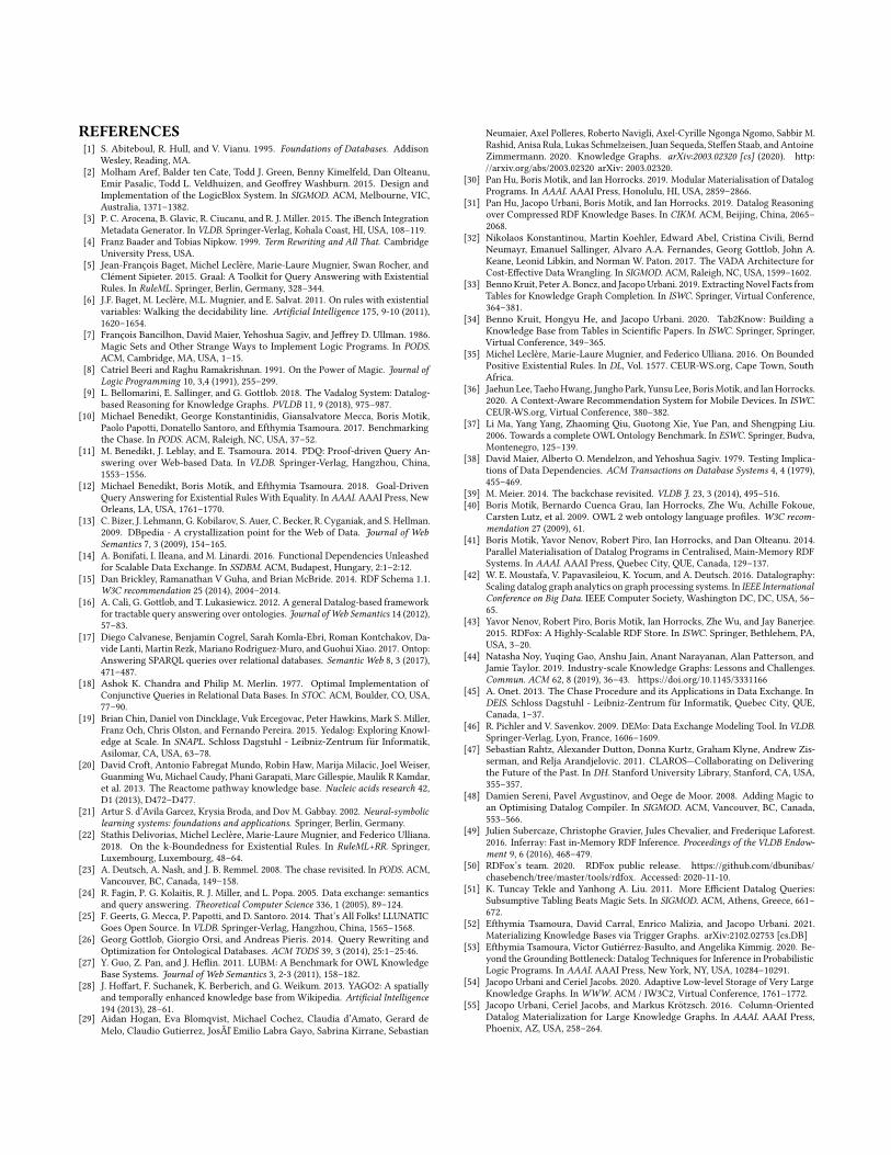
Figure 2: Different strategies for executing the rules from P2.
6.2 A more efficient rule execution strategyEG-rewritings can be further used to optimize the execution of the
rules as shown in the example below.
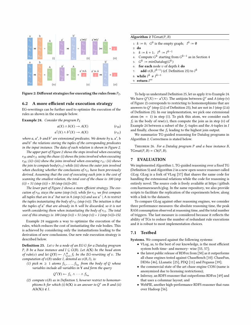
Example 24. Consider the program P2
a(X ) ∧ b(X ) → A(X ) (r10)
a′(X ) ∧ b ′(X ) → A(X ) (r11)
where a, a′, b and b ′ are extensional predicates. We denote by a, a′, band b′ the relations storing the tuples of the corresponding predicatesin the input instance. The data of each relation is shown in Figure 2.
The upper part of Figure 2 shows the steps involved when executingr10 and r11 using the chase: (i) shows the joins involved when executingr10; (ii)–(iii) show the joins involved when executing r11: (ii) showsthe join to compute body(r11) while (iii) shows the outer join involvedwhen checking whether the conclusions of r11 have been previouslyderived. Assuming that the cost of executing each join is the cost ofscanning the smallest relation, the total cost of the chase is: 100 (step(i)) + 51 (step (ii)) + 50 (step (iii))=201.
The lower part of Figure 2 shows a more efficient strategy. The exe-cution of r10 stays the same (step (iv)), while for r11 we first computeall tuples that are in a′ but not in A (step (v)) and use a′ \ A to restrictthe tuples instantiating the body of r11 (step (vi)). The intuition is thatthe tuples of a′ that are already in A will be discarded, so it is notworth considering them when instantiating the body of r11. The totalcost of this strategy is: 100 (step (iv)) + 51 (step (v)) + 1 (step (vi))=152.
Example 24 suggests a way to optimize the execution of the
rules, which reduces the cost of instantiating the rule bodies. This
is achieved by considering only the instantiations leading to the
derivation of new conclusions. Our new rule execution strategy is
described below.
Definition 25. Let v be a node of an EG G for a Datalog programP , B be a base instance and I ⊆ G(B). Let A(X) be the head atomof rule(v) and let Q(Y) ←
∧ni=1 fi be the EG-rewriting of v . The
computation of v(B) under I , denoted as v(B, I ), is:(1) pick m ≥ 1 atoms fi1 , . . . , fim from the body of Q whose
variables include all variables in Y and form the query
Q ′(Y) ← fi1 ∧ · · · ∧ fim
(2) compute v(B) as in Definition 5, however restrict to homomor-phisms h for which (i) h(X) is an answer to Q ′ on B and (ii)A(h(X)) < I .
Algorithm 2 TGmat(P ,B)
1: k ··= 0; G0is the empty graph; I0 ··= ∅
2: do3: k ··= k + 1; Ik ··= Ik−1
4: Compute Gkstarting from Gk−1
as in Section 4
5: Gk ··= minDatalog(Gk )
6: for each node v of depth k do7: add v(B, Ik−1) (cf. Definition 25) to Ik
8: while Ik , Ik−1
9: return I∞
To help us understand Definition 25, let us apply it to Example 24.
We have Q ′(X ) ← a′(X ). The antijoin between Q ′ and A (step (v)
of Figure 2) corresponds to restricting to homomorphisms that are
answers toQ ′ (step (2.i) of Definition 25), but are not in I (step (2.ii)
of Definition 25). In our implementation, we pick one extensional
atom (m = 1) in step (1). To pick this atom, we consider each
fi in the body of rew(v), then compute the join as in step (v) of
Example 24 between a subset of the fi -tuples and the A-tuples in Iand finally, choose the fi leading to the highest join output.
We summarize TG-guided reasoning for Datalog programs in
Algorithm 2. Correctness is stated below.
Theorem 26. For a Datalog program P and a base instance B,TGmat(P ,B) = Ch(P ,B).
7 EVALUATIONWe implemented Algorithm 1, TG-guided reasoning over a fixed TG
(Definition 5) and Algorithm 2 in a new open-source reasoner called
GLog. GLog is a fork of VLog [57] that shares the same code for
handling the extensional relations while the code for reasoning is
entirely novel. The source code is freely available at https://github.
com/karmaresearch/glog. In the same repository, we also provide
scripts to facilitate the replication of the experiments below, along
with a link to the datasets.
To compare GLog against other reasoning engines, we consider
three performance measures: the absolute reasoning time, the peak
RAMconsumption observed at reasoning time, and the total number
of triggers. The last measure is considered because it reflects the
ability of TGs to reduce the number of redundant rule executions
and it is robust to most implementation choices.
7.1 TestbedSystems.We compared against the following systems:
• VLog, as, to the best of our knowledge, is the most efficient
system both time- and memory- wise [55, 57];
• the latest public release of RDFox from [50] as it outperforms
all chase engines tested against ChaseBench [10]: ChaseFun,
DEMo [46], LLunatic [25], PDQ [11] and Pegasus [39];
• the commercial state of the art chase engine COM (name is
anonymized due to licensing restrictions);
• Inferray, an RDFS reasoner that outperforms RDFox [49] and
that uses a columnar layout; and
• WebPIE, another high-performance RDFS reasoner that runs
over Hadoop [56].

Table 1: The considered benchmarks. #EDP’s and #IDP’s ab-solute numbers are stated in millions of facts.
#Rules #IDP’sScenario #EDP’s LI L LE LI L LE
Linear and Datalog scenariosLUBM var. 163 170 182 116% 120% 232%
UOBM 2.1 337 561 NA 3.5 3.9 NA
DBpedia 29 4204 9396 NA 31.9 33.1 NA
Claros 13.8 1749 2689 2749 65.8 8.9 548
React. 5.6 259 NA NA 11.3 NA NA
ChaseBench scenariosSTB-128 0.15 167 1.9
ONT-256 1 529 5.6
RDFS (ρDF) scenariosLUBM 16.7 160 18
YAGO 18.2 498016 27
We ran VLog, RDFox and the commercial chase engine COM
using their most efficient chase implementations. For VLog, this is
the restricted chase, while for RDFox and COM this is the Skolem
one [10]. All engines ran using a single thread. We could not obtain
access to the Vadalog [9] binaries. However, we perform an indirect
comparison against Vadalog: we both compare against RDFox using
the ChaseBench scenarios from [10].
Benchmarks. To asses the performance of GLog on linear and
Datalog scenarios, we considered benchmarks previously used to
evaluate reasoners, including VLog, RDFox, among others. LUBM
[27] and UOBM [37] are synthetic benchmarks; DBpedia [13] (v2014,
available online1) is a popular KB built fromWikipedia; Claros [47]
and Reactome [20] are real-world ontologies2. For the linear sce-
narios, both VLog and GLog access the KBs stored as a collection
of CSV files. For the Datalog scenarios, the KBs are stored instead
with the RDF engine Trident [54].
Linear scenarios. Linear scenarios were created using LUBM,
UOBM, DBpedia, Claros and Reactome. For the first four KBs, we
considered the linear rules returned by translating the OWL on-
tologies in each KB using the method described by [58], which was
the technique used for evaluating our competitors [41, 55]. This
method converts an OWL ontology O into a Datalog program PLsuch that O |= PL . For instance, the OWL axiom A ⊑ B (concept
inclusion) is translated into the rule A(X ) → B(X ). This techniqueis ideal for our purposes since this subset is what is mostly sup-
ported by RDF reasoners [41]. Here, the subscript “L” stands for
“lower bound”. In fact, not every ontology can be fully captured
by Datalog (e.g., ontologies that are not in OWL 2 RL) and in such
cases the translation captures a subset of all possible derivations.
For Reactome, we considered the subset of linear rules from the
program used in [57]. The programs for the first four KBs do not
include any existential rules while the program for Reactome does.
Linear scenarios are suffixed by “LI”, e.g., LUBM-LI.
Datalog scenarios. Datalog scenarios were created using LUBM,
UOBM, DBpedia and Claros, as Reactome includes non-Datalog
rules only. LUBM comes with a generator, which allows controlling
the size of the base instance by fixing the number of different
1https://www.cs.ox.ac.uk/isg/tools/RDFox/2014/AAAI/input/DBpedia/ttl/
2Both datasets are available in our data repository.
universities X in the instance. One university roughly corresponds
to 132k facts. In our experiments, we set X to the following values:
125, 1k, 2k, 4k, 8k, 32k, 64k, 128k. This means that our largest KB
contains about 17B facts. As programs, we used the entire Datalog
programs (linear and non-linear) obtained with [58] as described
above. These programs are suffixed by “L”. For Claros and LUBM,we
used two additional programs, suffixed by “LE”, created by [41] as
harder benchmarks. These programs extend the “L” ones with extra
rules, such as the transitive and symmetric rules for owl:sameAs.The relationship between the various rulesets is LI ⊂ L ⊂ LE.
ChaseBench scenarios. ChaseBench was introduced for evaluat-
ing the performance of chase engines [10]. The benchmark comes
with four different families of scenarios. Out of these four families,
we focused on the iBench scenarios, namely STB-128 and ONT-
256 [3], because they come with non-linear rules with existentials
that involve many joins and that are highly recursive. Moreover,
as we do compare against RDFox, which was the top-performing
chase engine in [10], we can use these two scenarios to indirectly
compare against all the engines considered in [10].
RDFS scenarios. In the Semantic Web, it has been shown that a
large part of the inference that is possible under the RDF Schema
(RDFS) [15] can be captured into a set of Datalog rules. A number
of works have focused on the execution of such rules. In particu-
lar, WebPIE and more recently Inferray returned state-of-the-art
performance for ρDF—a subset of RDFS that captures its essentialsemantics. It is interesting to compare the performance of GLog,
which is a generic engine not optimized for RDFS rules, against
such ad-hoc systems. To this end, we considered YAGO [28] and a
LUBM KB with 16.7M triples. As rules for GLog, we translated the
ontologies under the ρDF semantics.
Table 1 shows, for each scenario, the corresponding number of
rules and EDP-facts as well as the number of IDP-facts in the model
of the KB. With LUBM and the linear and Datalog scenarios, the
number of IDP-facts is proportional to the input size, thus it is
stated as %. For instance, with the “LI” rules, the output is 116%,
which means that if the input contains 1M facts, then reasoning
returns 1.16M new facts.
Hardware. All experiments except the ones on scalability (Sec-
tion 7.5) ran on an Ubuntu 16.04 Linux PC with Intel i7 64-bit CPU
and 94.1 GiB RAM. For our experiments on scalability, we used a
second machine with an Intel Xeon E5 and 256 GiB of RAM due to
the large sizes of the KBs. The cost of both machines is <$5k, thus
we arguably label them as commodity hardware.
7.2 Results for linear scenariosTable 2 summarizes the results of our empirical evaluation for the
linear scenarios. Recall that when a program is linear and FES itadmits a finite TG, which can be computed prior to reasoning
using tglinear (Algorithm 1) and minimized using minLinear fromDefinition 15. Columns two to seven show the runtime and the peak
memory consumption for VLog, RDFox and the commercial engine
COM. The remaining columns show results related to TG-guided
reasoning. Column Comp. shows the time to compute and minimize
a TG using tglinear andminLinear. Column Reason shows the time
to reason over the computed TG given a base instance (i.e., apply
Definition 5). Column w/o cleaning shows the total runtime if we
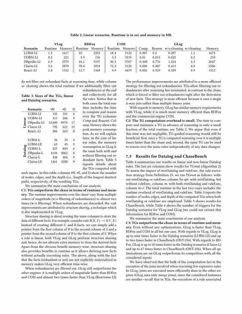
Table 2: Linear scenarios. Runtime is in sec and memory in MB.
VLog RDFox COM GLogScenario Runtime Memory Runtime Memory Runtime Memory Comp. Reason w/o cleaning w/cleaning Memory
LUBM-LI 1.3 1617 22 2353 18.4 5122 0.007 0.2 0.207 1.1 1674
UOBM-LI 0.3 221 3.9 726 3.3 3570 0.01 0.015 0.025 0.2 219
DBpedia-LI 6.9 2579 44.1 3197 36.3 3767 0.448 0.776 1.224 4.5 2647
Claros-LI 5.6 2870 78.4 3918 72.3 5122 0.006 0.407 0.413 4.8 2586
React.-LI 1.8 1312 12.7 1448 9.9 4479 0.002 0.329 0.329 0.9 1312
do not filter out redundant facts at reasoning time, while column
w/ cleaning shows the total runtime if we additionally filter out
Table 3: Sizes of the TGs, linearand Datalog scenarios.
Scenario #N #E D
Line
ar
LUBM-LI 155 101 6
UOBM-LI 313 206 9
DBpedia-LI 12 600 8970 17
Claros-LI 792 621 23
React.-LI 386 263 8
Datalog
LUBM-L 56 33 4
LUBM-LE 63 43 5
UOBM-L 527 859 6
DBpedia-L 4144 3062 8
Claros-L 438 404 9
Claros-LE 1461 3288 9
redundancies at the end
and collectively for all
the rules. Notice that in
both cases the total run-
time includes the time
to compute and reason
over the TG (columns
Comp and Reason). Col-umnMemory shows the
peak memory consump-
tion. As we will explain
later, in the case of lin-
ear rules, the memory
consumption in GLog is
the same both with and
without filtering out re-
dundant facts. Table 3
reports details about
the TGs computed with
such inputs. In this table, columns #N, #E, and D show the number
of nodes, edges, and the depth (i.e., length of the longest shortest
path), respectively, of the resulting TGs.
We summarize the main conclusions of our analysis.
C1: TGs outperform the chase in terms of runtime andmem-ory. The runtime improvements over the chase vary from multiple
orders of magnitude (w/o filtering of redundancies) to almost two
times (w/o filtering). When redundancies are discarded, the vast
improvements are attributed to structure sharing, a technique whichis also implemented in VLog.
Structure sharing is about reusing the same columns to store the
data of different facts. For example, consider ruleR(X ,Y ) → S(Y ,X ).Instead of creating different S- and R-facts, we can simply add a
pointer from the first column of R to the second column of S and a
pointer from the second column of R to the first column of S . When
a rule is linear, both VLog and GLog perform structure sharing
and, hence, do not allocate extra memory to store the derived facts.
Apart from the obvious benefit memory-wise, structure sharing
also provides benefits in runtime as it allows deriving new facts
without actually executing rules. The above, along with the fact
that the facts (redundant or not) are not explicitly materialized in
memory makes GLog very efficient time-wise.
When redundancies are filtered out, GLog still outperforms the
other engines: it is multiple orders of magnitude faster than RDFox
and COM and almost two times faster than VLog (Reactome-LI).
The performance improvements are attributed to a more efficient
strategy for filtering out redundancies: TGs allow filtering out re-
dundancies after reasoning has terminated, in contrast to the chase,
which is forced to filter out redundancies right after the derivation
of new facts. This strategy is more efficient because it uses a single
n-way join rather than multiple binary joins.
With regards tomemory, GLog has similar memory requirements
with VLog, while it is much more memory efficient than RDFox
and the commercial engine COM.
C2: The TG computation overhead is small. The time to com-
pute and minimize a TG in advance of reasoning is only a small
fraction of the total runtime, see Table 2. We argue that even if
this time was not negligible, TG-guided reasoning would still be
beneficial: first, once a TG is computed reasoning over it is multiple
times faster than the chase and, second, the same TG can be used
to reason over the same rules independently of any data changes.
7.3 Results for Datalog and ChaseBenchTable 4 summarizes our results on linear and non-linear Datalog
rules. The last six columns show results for TGmat (Algorithm 2).
To assess the impact of minDatalog and ruleExec, the rule execu-tion strategy from Definition 25, we ran TGmat as follows: with-out minDatalog or ruleExec, column No opt; with minDatalog, butwithout ruleExec, column m; with both minDatalog and ruleExec,column m+r. The total runtime in the last two cases includes the
runtime overhead of minDatalog and ruleExec. Table 3 reports thenumber of nodes, edges, and depth of the computed TGs when both
minDatalog or ruleExec are employed. Table 5 shows results for
ChaseBench, while Table 6 shows the number of triggers for the
Datalog scenarios for VLog and GLog (we could not extract this
information for RDFox and COM).
We summarize the main conclusions of our analysis.
C3: TGs outperform the chase in terms of runtime andmem-ory. Even without any optimizations, GLog is faster than VLog,
RDFox and COM in all but one case. With regards to VLog, GLog is
up to nine times faster in the Datalog scenarios (LUBM-LE) and up
to two times faster in ChaseBench (ONT-256). With regards to RD-
Fox, GLog is up to 20 times faster in the Datalog scenarios (Claros-L)
and up to 67 times faster in ChaseBench (ONT-256). When all op-
timizations are on GLog outperforms its competitors with all the
considered inputs.
We have observed that the bulk of the computation lies in the
execution of the joins involved when executing few expensive rules.
In GLog, joins are executed more efficiently than in the other en-
gines (GLog uses only merge joins), since the considered instances
are smaller—recall that in TGs, the execution of a rule associated

Table 4: Datalog scenarios. Runtime is in sec and memory in MB. ∗ denotes timeout after 1h.
VLog RDFox COM GLog Runtime GLog MemoryScenario Runtime Memory Runtime Memory Runtime Memory No opt m m+r No opt m m+r
LUBM-L 1.5 324 23 2301 20.4 4479 2.4 2.2 1.0 446 424 264
LUBM-LE 170.5 2725 116.6 3140 115.9 3610 17.3 17.2 16.1 1340 1310 1338
UOBM-L 7.3 1021 10 784 10 4215 2.6 2.4 2.6 335 335 342
DBpedia-L 41.6 827 64.4 3290 198.4 3878 20 19 19 1341 1352 1339
Claros-L 431 3170 2512 5491 2373.0 6453 122 118.3 119 6076 6077 6078
Claros-LE 2771.8 11 895 * * * * 1040.8 1012.2 1053.9 48 464 48 474 48 455
Table 5: ChaseBench scenarios. Runtime in sec and memory in MB.
VLog RDFox COM GLog TG SizesScenario Runtime Memory Runtime Memory Runtime Memory Runtime Memory #N #E D
STB-128 0.5 1350 13.4 1747 10 5217 0.2 1266 192 0 0
ONT-256 2.3 4930 49 3997 35 6340 1 4930 577 65 3
Table 6: #Triggers (millions), Datalog scenarios.
VLog GLogScenario no opt m m+r
LUBM-L 38 32 29 25
LUBM-LE 239 100 98 93
UOBM-L 47 9 8 8
DBpedia-L 79 63 61 47
Claros-L 286 218 195 185
Claros-LE 1099 1072 1049 1039
Table 7: RDFS scenarios (L=LUBM, Y=YAGO). Runtime in secand memory in MB.
WebPIE Inferray GLog TG SizesS Run. Mem. Run. Mem. Run. Mem. #N #E D
L 338 1124 39 7000 0.3 186 53 25 4
Y 745 1075 116.6 14 000 25 1603 1.07M 888k 20
with a node v considers only the instances of the parents of v . Dueto the above, the optimizations do not decrease the runtime con-
siderably. The only exception is LUBM-L, where the optimizations
half the runtime.
Continuing with the optimizations, their runtime overhead is
very low: it is 9% of the total runtime (LUBM-L), while the overhead
of minDatalog is less than 1% of the total runtime (detailed results
are in [52]). We consider this overhead to be acceptable, since, as we
shall see later, the optimizations considerably decrease the number
of triggers, a performance measure which is robust to hardware
and most implementation choices.
It is important to mention that GLog implements the technique
in [30] for executing transitive and symmetric rules. The improve-
ments brought by this technique are most visible with LUBM-LE
where the runtime increases from 18s with this technique to 71s
without it. Other improvements occur with UOBM-L and DBpedia-L
(69% and 57% respectively). In any case, even without this technique,
GLog remains faster than its competitors in all cases. Detailed re-
sults can be found in [52].
Last, the ChaseBench experiments allow us to compare against
Vadalog. According to [9], Vadalog is three times faster than RDFox
on STB-128 and ONT-256. Our empirical results show that GLog
brings more substantial runtime improvements: GLog is from 49
times to more than 67 times faster than RDFox in those scenarios.
With regards to memory, the memory footprint of GLog again
is comparable to that of VLog and it is lower than that of RDFox
and of COM.
C4: TGs outperform the chase in terms of the number of trig-gers. Table 6 shows that the total number of triggers produced with
the Datalog rules. Recall that the number of triggers is a good indi-
cator for estimating the amount of redundant computations. From
the table, we see that this number is considerably lower than the
total number of triggers in VLog even when the optimizations are
disabled. This is due to the different approaches employed to fil-
ter out redundancies: VLog filters out redundancies right after the
execution of each rule [55], while GLog performs this filtering af-
ter each round. When the optimizations are enabled, the number
of triggers further decreases: in the best case (DBpedia-L), GLog
computes 1.69 times fewer triggers (79M/47M).
7.4 Results for RDFS scenariosTable 7 summarizes the results of the RDFS scenarios where GLog
is configured with both optimizations enabled. We can see that
GLog is faster than both RDFS engines. With regards to Inferray,
GLog is two orders of magnitude faster on LUBM and more than
four times faster on YAGO. With regards to WebPIE, GLog is three
orders of magnitude faster on LUBM and more than 32 times faster
on YAGO. With regards to memory, GLog is more memory efficient
in all but one case.
7.5 Results on scalabilityWe used the LUBM benchmark to create several KBs with 133M,
267M, 534M, 1B, 2B, 4B, 8B, and 17B facts respectively. Table 8

Table 8: Scalability results. Runtime in sec, memory in GB.
133M 267M 534M 1B 2B 4B 8B 17B
Run. 13 27 56 203 226 520 993 2272
Mem 1 3 6 23 34 49 98 174
#IDP’s 160M 320M 641M 1B 2B 5B 10B 20B
summarizes the performance with the Datalog program LUBM-
L. Columns are labeled with the size of the input database. Each
column shows the runtime, the peak memory consumption, and
the number of derived facts for each input database. We can see
that GLog can reason on a KB with up to 17B facts in less than
40 minutes without resorting to expensive hardware. We are not
aware of any other centralized reasoning engine that scales up to
such an extent.
8 RELATEDWORKWe briefly discuss different approaches adopted in the literature
for improving the performance of the chase, and we compare them
with our approach.
One approach to improve the reasoning performance is to paral-
lelize the execution of the rules. RDFOx proposes a parallelization
technique for Datalog materialization with mostly lock-free data
insertion. Parallelization has been also been studied for reasoning
over RDFS and OWL ontologies. For example, WebPIE encodes the
materialization process into a set of MapReduce programs while
Inferray executes each rule on a dedicated thread. Our experiments
show that GLog outperforms all these engines in a single-core sce-
nario. This motivates further research on parallelizing TG-based
materialization.
A second approach to improve the reasoning performance is to
reduce the number of logically redundant facts by appropriately
ordering the rules. In [56], the authors describe a rule ordering that
is optimal only for a fixed set of RDFS rules. In contrast, we focus
on generic programs. ChaseFun [14] proposes a new rule ordering
technique that focuses on equality generating dependencies. Hence,it is orthogonal to our approach. In a similar spirit, the rewriting
technique from [30] targets transitive and symmetric rules. GLog
applies this technique by default to improve the performance, but
our experiments show it outperforms the state of the art even
without this optimization.
To optimize the execution of the rules themselves, most chase
engines rely on external DBMSs or employ state of the art query
execution algorithms: LLunatic [25], PDQ and ChaseFun run on top
of PostgreSQL; RDFox and VLog implement their own in-memory
rule execution engines. However, none of these engines can effec-
tively reduce the instances over which rules are executed as TGs
do. Other approaches involve exploring columnar memory layouts
as in VLog and Inferray to reduce memory consumption and to
guarantee sequential access and efficient sort-merge join inference.
Orthogonal to the above is the work in [9], which introduces
a new chase variant for materializing KBs of warded Datalog pro-
grams. Warded Datalog is a class of programs not admiting a finite
model for any base instance. The variant works as the restricted
chase does but replaces homomorphism with isomorphism checks.
As a result, the computed models become bigger. An implementa-
tion of the warded chase is also introduced in [9], which focuses
on decreasing the cost of isomorphism checks. The warded chase
implementation does not apply any techniques to detect redundan-
cies in the offline fashion as we do for linear rules, or to reduce the
execution cost of Datalog rules as we do in Section 6.
We now turn our attention to the applications of materializa-
tion in goal-driven query answering. Two well-known database
techniques that use materialization as a tool for goal-driven query
answering are magic sets and subsumptive tabling [7, 8, 48, 51]. The
advantage of these techniques over the query rewriting ones, whichare not based on materialization, e.g., [5, 17, 26], is the full support
of Datalog. The query rewriting techniques can support Datalog
of bounded recursion only. Beyond Datalog, materialization-based
techniques have been recently proposed for goal-driven query an-
swering over KBs with equality [12], as well as for probabilistic KBs
[53], leading in both cases to significant improvements in terms
of runtime and memory consumption. The above automatically
turns TGs to a very powerful tool to also support query-driven
knowledge exploration.
TGs are different from acyclic graphs of rule dependencies [6]:
the former contain a single node per rule while TGs do not.
9 CONCLUSIONWe introduced a novel approach for materializing KBs that is based
on traversing acyclic graphs of rules called TGs, and implemented
it into a new reasoner called GLog. The primary goal of TGs is to
reduce the amount of redundant computations performed during
the execution of a chase algorithm. Our theoretical analysis and
empirical evaluation over well-known benchmarks show that TG-
guided reasoning is a more efficient alternative to the chase, since it
effectively overcomes all of its limitations. In particular, our experi-
ments report that GLog often outperforms existing state-of-the-art
engines in terms of runtime and memory consumption. Moreover,
in our largest experiment GLog was able to materialize a KB with
17B facts in less than an hour using commodity hardware. In terms
of scalability, these are unprecedented results, as far as we know.
There are multiple research directions that are worth pursu-
ing, either to further improve the performance or to extend the
applicability of TGs to more scenarios. First, studying how TGs
can be efficiently updated in response to KB updates is a natural
continuation of our work. Further work is also needed to under-
stand whether TGs can be computed using distributed computing
architectures. Finally, it is interesting to study whether TGs can be
combined with query rewriting techniques to further improve the
performance of query answering.
Acknowledgments. David Carral conducted this research at TU
Dresden, where he was supported by Deutsche Forschungsgemein-
schaft (DFG, German Research Foundation) in projects number
389792660 (TRR 248, Center for Perspicuous Systems) and KR
4381/1-1 (Emmy Noether grant DIAMOND), and by the Bundesmin-
isterium für Bildung und Forschung (BMBF, Federal Ministry of
Education and Research) in the Center for Scalable Data Analytics
and Artificial Intelligence (ScaDS.AI).
REFERENCES[1] S. Abiteboul, R. Hull, and V. Vianu. 1995. Foundations of Databases. Addison
Wesley, Reading, MA.
[2] Molham Aref, Balder ten Cate, Todd J. Green, Benny Kimelfeld, Dan Olteanu,
Emir Pasalic, Todd L. Veldhuizen, and Geoffrey Washburn. 2015. Design and
Implementation of the LogicBlox System. In SIGMOD. ACM, Melbourne, VIC,
Australia, 1371–1382.
[3] P. C. Arocena, B. Glavic, R. Ciucanu, and R. J. Miller. 2015. The iBench Integration
Metadata Generator. In VLDB. Springer-Verlag, Kohala Coast, HI, USA, 108–119.[4] Franz Baader and Tobias Nipkow. 1999. Term Rewriting and All That. Cambridge
University Press, USA.
[5] Jean-François Baget, Michel Leclère, Marie-Laure Mugnier, Swan Rocher, and
Clément Sipieter. 2015. Graal: A Toolkit for Query Answering with Existential
Rules. In RuleML. Springer, Berlin, Germany, 328–344.
[6] J.F. Baget, M. Leclère, M.L. Mugnier, and E. Salvat. 2011. On rules with existential
variables: Walking the decidability line. Artificial Intelligence 175, 9-10 (2011),1620–1654.
[7] François Bancilhon, David Maier, Yehoshua Sagiv, and Jeffrey D. Ullman. 1986.
Magic Sets and Other Strange Ways to Implement Logic Programs. In PODS.ACM, Cambridge, MA, USA, 1–15.
[8] Catriel Beeri and Raghu Ramakrishnan. 1991. On the Power of Magic. Journal ofLogic Programming 10, 3,4 (1991), 255–299.
[9] L. Bellomarini, E. Sallinger, and G. Gottlob. 2018. The Vadalog System: Datalog-
based Reasoning for Knowledge Graphs. PVLDB 11, 9 (2018), 975–987.
[10] Michael Benedikt, George Konstantinidis, Giansalvatore Mecca, Boris Motik,
Paolo Papotti, Donatello Santoro, and Efthymia Tsamoura. 2017. Benchmarking
the Chase. In PODS. ACM, Raleigh, NC, USA, 37–52.
[11] M. Benedikt, J. Leblay, and E. Tsamoura. 2014. PDQ: Proof-driven Query An-
swering over Web-based Data. In VLDB. Springer-Verlag, Hangzhou, China,1553–1556.
[12] Michael Benedikt, Boris Motik, and Efthymia Tsamoura. 2018. Goal-Driven
Query Answering for Existential Rules With Equality. In AAAI. AAAI Press, NewOrleans, LA, USA, 1761–1770.
[13] C. Bizer, J. Lehmann, G. Kobilarov, S. Auer, C. Becker, R. Cyganiak, and S. Hellman.
2009. DBpedia - A crystallization point for the Web of Data. Journal of WebSemantics 7, 3 (2009), 154–165.
[14] A. Bonifati, I. Ileana, and M. Linardi. 2016. Functional Dependencies Unleashed
for Scalable Data Exchange. In SSDBM. ACM, Budapest, Hungary, 2:1–2:12.
[15] Dan Brickley, Ramanathan V Guha, and Brian McBride. 2014. RDF Schema 1.1.
W3C recommendation 25 (2014), 2004–2014.
[16] A. Calì, G. Gottlob, and T. Lukasiewicz. 2012. A general Datalog-based framework
for tractable query answering over ontologies. Journal of Web Semantics 14 (2012),57–83.
[17] Diego Calvanese, Benjamin Cogrel, Sarah Komla-Ebri, Roman Kontchakov, Da-
vide Lanti, Martin Rezk, Mariano Rodriguez-Muro, and Guohui Xiao. 2017. Ontop:
Answering SPARQL queries over relational databases. Semantic Web 8, 3 (2017),471–487.
[18] Ashok K. Chandra and Philip M. Merlin. 1977. Optimal Implementation of
Conjunctive Queries in Relational Data Bases. In STOC. ACM, Boulder, CO, USA,
77–90.
[19] Brian Chin, Daniel von Dincklage, Vuk Ercegovac, Peter Hawkins, Mark S. Miller,
Franz Och, Chris Olston, and Fernando Pereira. 2015. Yedalog: Exploring Knowl-
edge at Scale. In SNAPL. Schloss Dagstuhl - Leibniz-Zentrum für Informatik,
Asilomar, CA, USA, 63–78.
[20] David Croft, Antonio Fabregat Mundo, Robin Haw, Marija Milacic, Joel Weiser,
GuanmingWu, Michael Caudy, Phani Garapati, Marc Gillespie, Maulik R Kamdar,
et al. 2013. The Reactome pathway knowledge base. Nucleic acids research 42,
D1 (2013), D472–D477.
[21] Artur S. d’Avila Garcez, Krysia Broda, and Dov M. Gabbay. 2002. Neural-symboliclearning systems: foundations and applications. Springer, Berlin, Germany.
[22] Stathis Delivorias, Michel Leclère, Marie-Laure Mugnier, and Federico Ulliana.
2018. On the k-Boundedness for Existential Rules. In RuleML+RR. Springer,Luxembourg, Luxembourg, 48–64.
[23] A. Deutsch, A. Nash, and J. B. Remmel. 2008. The chase revisited. In PODS. ACM,
Vancouver, BC, Canada, 149–158.
[24] R. Fagin, P. G. Kolaitis, R. J. Miller, and L. Popa. 2005. Data exchange: semantics
and query answering. Theoretical Computer Science 336, 1 (2005), 89–124.[25] F. Geerts, G. Mecca, P. Papotti, and D. Santoro. 2014. That’s All Folks! LLUNATIC
Goes Open Source. In VLDB. Springer-Verlag, Hangzhou, China, 1565–1568.[26] Georg Gottlob, Giorgio Orsi, and Andreas Pieris. 2014. Query Rewriting and
Optimization for Ontological Databases. ACM TODS 39, 3 (2014), 25:1–25:46.[27] Y. Guo, Z. Pan, and J. Heflin. 2011. LUBM: A Benchmark for OWL Knowledge
Base Systems. Journal of Web Semantics 3, 2-3 (2011), 158–182.[28] J. Hoffart, F. Suchanek, K. Berberich, and G. Weikum. 2013. YAGO2: A spatially
and temporally enhanced knowledge base from Wikipedia. Artificial Intelligence194 (2013), 28–61.
[29] Aidan Hogan, Eva Blomqvist, Michael Cochez, Claudia d’Amato, Gerard de
Melo, Claudio Gutierrez, JosÃľ Emilio Labra Gayo, Sabrina Kirrane, Sebastian
Neumaier, Axel Polleres, Roberto Navigli, Axel-Cyrille Ngonga Ngomo, Sabbir M.
Rashid, Anisa Rula, Lukas Schmelzeisen, Juan Sequeda, Steffen Staab, and Antoine
Zimmermann. 2020. Knowledge Graphs. arXiv:2003.02320 [cs] (2020). http:
//arxiv.org/abs/2003.02320 arXiv: 2003.02320.
[30] Pan Hu, Boris Motik, and Ian Horrocks. 2019. Modular Materialisation of Datalog
Programs. In AAAI. AAAI Press, Honolulu, HI, USA, 2859–2866.[31] Pan Hu, Jacopo Urbani, Boris Motik, and Ian Horrocks. 2019. Datalog Reasoning
over Compressed RDF Knowledge Bases. In CIKM. ACM, Beijing, China, 2065–
2068.
[32] Nikolaos Konstantinou, Martin Koehler, Edward Abel, Cristina Civili, Bernd
Neumayr, Emanuel Sallinger, Alvaro A.A. Fernandes, Georg Gottlob, John A.
Keane, Leonid Libkin, and Norman W. Paton. 2017. The VADA Architecture for
Cost-Effective Data Wrangling. In SIGMOD. ACM, Raleigh, NC, USA, 1599–1602.
[33] Benno Kruit, Peter A. Boncz, and Jacopo Urbani. 2019. Extracting Novel Facts from
Tables for Knowledge Graph Completion. In ISWC. Springer, Virtual Conference,364–381.
[34] Benno Kruit, Hongyu He, and Jacopo Urbani. 2020. Tab2Know: Building a
Knowledge Base from Tables in Scientific Papers. In ISWC. Springer, Springer,Virtual Conference, 349–365.
[35] Michel Leclère, Marie-Laure Mugnier, and Federico Ulliana. 2016. On Bounded
Positive Existential Rules. In DL, Vol. 1577. CEUR-WS.org, Cape Town, South
Africa.
[36] Jaehun Lee, TaehoHwang, Jungho Park, Yunsu Lee, BorisMotik, and IanHorrocks.
2020. A Context-Aware Recommendation System for Mobile Devices. In ISWC.CEUR-WS.org, Virtual Conference, 380–382.
[37] Li Ma, Yang Yang, Zhaoming Qiu, Guotong Xie, Yue Pan, and Shengping Liu.
2006. Towards a complete OWL Ontology Benchmark. In ESWC. Springer, Budva,Montenegro, 125–139.
[38] David Maier, Alberto O. Mendelzon, and Yehoshua Sagiv. 1979. Testing Implica-
tions of Data Dependencies. ACM Transactions on Database Systems 4, 4 (1979),455–469.
[39] M. Meier. 2014. The backchase revisited. VLDB J. 23, 3 (2014), 495–516.[40] Boris Motik, Bernardo Cuenca Grau, Ian Horrocks, Zhe Wu, Achille Fokoue,
Carsten Lutz, et al. 2009. OWL 2 web ontology language profiles. W3C recom-mendation 27 (2009), 61.
[41] Boris Motik, Yavor Nenov, Robert Piro, Ian Horrocks, and Dan Olteanu. 2014.
Parallel Materialisation of Datalog Programs in Centralised, Main-Memory RDF
Systems. In AAAI. AAAI Press, Quebec City, QUE, Canada, 129–137.[42] W. E. Moustafa, V. Papavasileiou, K. Yocum, and A. Deutsch. 2016. Datalography:
Scaling datalog graph analytics on graph processing systems. In IEEE InternationalConference on Big Data. IEEE Computer Society, Washington DC, DC, USA, 56–
65.
[43] Yavor Nenov, Robert Piro, Boris Motik, Ian Horrocks, Zhe Wu, and Jay Banerjee.
2015. RDFox: A Highly-Scalable RDF Store. In ISWC. Springer, Bethlehem, PA,
USA, 3–20.
[44] Natasha Noy, Yuqing Gao, Anshu Jain, Anant Narayanan, Alan Patterson, and
Jamie Taylor. 2019. Industry-scale Knowledge Graphs: Lessons and Challenges.
Commun. ACM 62, 8 (2019), 36–43. https://doi.org/10.1145/3331166
[45] A. Onet. 2013. The Chase Procedure and its Applications in Data Exchange. In
DEIS. Schloss Dagstuhl - Leibniz-Zentrum für Informatik, Quebec City, QUE,
Canada, 1–37.
[46] R. Pichler and V. Savenkov. 2009. DEMo: Data Exchange Modeling Tool. In VLDB.Springer-Verlag, Lyon, France, 1606–1609.
[47] Sebastian Rahtz, Alexander Dutton, Donna Kurtz, Graham Klyne, Andrew Zis-
serman, and Relja Arandjelovic. 2011. CLAROS—Collaborating on Delivering
the Future of the Past. In DH. Stanford University Library, Stanford, CA, USA,
355–357.
[48] Damien Sereni, Pavel Avgustinov, and Oege de Moor. 2008. Adding Magic to
an Optimising Datalog Compiler. In SIGMOD. ACM, Vancouver, BC, Canada,
553–566.
[49] Julien Subercaze, Christophe Gravier, Jules Chevalier, and Frederique Laforest.
2016. Inferray: Fast in-Memory RDF Inference. Proceedings of the VLDB Endow-ment 9, 6 (2016), 468–479.
[50] RDFox’s team. 2020. RDFox public release. https://github.com/dbunibas/
chasebench/tree/master/tools/rdfox. Accessed: 2020-11-10.
[51] K. Tuncay Tekle and Yanhong A. Liu. 2011. More Efficient Datalog Queries:
Subsumptive Tabling Beats Magic Sets. In SIGMOD. ACM, Athens, Greece, 661–
672.
[52] Efthymia Tsamoura, David Carral, Enrico Malizia, and Jacopo Urbani. 2021.
Materializing Knowledge Bases via Trigger Graphs. arXiv:2102.02753 [cs.DB]
[53] Efthymia Tsamoura, Víctor Gutiérrez-Basulto, and Angelika Kimmig. 2020. Be-
yond the Grounding Bottleneck: Datalog Techniques for Inference in Probabilistic
Logic Programs. In AAAI. AAAI Press, New York, NY, USA, 10284–10291.
[54] Jacopo Urbani and Ceriel Jacobs. 2020. Adaptive Low-level Storage of Very Large
Knowledge Graphs. In WWW. ACM / IW3C2, Virtual Conference, 1761–1772.
[55] Jacopo Urbani, Ceriel Jacobs, and Markus Krötzsch. 2016. Column-Oriented
Datalog Materialization for Large Knowledge Graphs. In AAAI. AAAI Press,Phoenix, AZ, USA, 258–264.

[56] Jacopo Urbani, Spyros Kotoulas, Jason Maassen, Frank van Harmelen, and Henri
Bal. 2010. OWL Reasoning with WebPIE: Calculating the Closure of 100 Billion
Triples. In ESWC. Springer, Heraklion, Greece, 213–227.[57] Jacopo Urbani, Markus KrÃűtzsch, Ceriel Jacobs, Irina Dragoste, and David Carral.
2018. Efficient Model Construction for Horn Logic with VLog. In IJCAR. Springer,
Oxford, UK, 680–688.
[58] Yujiao Zhou, Bernardo Cuenca Grau, Ian Horrocks, Zhe Wu, and Jay Banerjee.
2013. Making the Most of your Triple Store: Query Answering in OWL 2 using
an RL Reasoner. In WWW. International World Wide Web Conferences Steering
Committee / ACM, Rio de Janeiro, Brazil, 1569–1580.