Materialism on the March: From conspicuous leisure to conspicuous consumption?

The Journal of Socio-Economics 37 (2008) 1937–1945

Contents lists available at ScienceDirect

The Journal of Socio-Economics

journa l homepage: www.e lsev ier .com/ locate /soceco

Materialism on the March: From conspicuous leisure to conspicuousconsumption?

Paul Frijtersa, Andrew Leighb,∗

a Queensland University of Technology, School of Economics and Finance, GPO Box 2434, Brisbane, QLD 4001, Australiab Australian National University, Research School of Social Sciences, HC Coombs Building, ACT 0200, Australia

a r t i c l e i n f o

Article history:Received 4 February 2008Received in revised form 13 May 2008Accepted 8 July 2008

JEL classification:J22J61D10D60B15

Keywords:Conspicuous consumptionConspicuous leisureMaterialismLabor supplyMobilityStatus

a b s t r a c t

This paper inserts Veblen’s [Veblen, T., 1898, The Theory of the Leisure Class. The VikingPress, New York] concepts of conspicuous leisure and conspicuous consumption into a verysimple model. Individuals have the choice to either invest their time into working, leadingto easily observable levels of consumption, or into conspicuous leisure, whose effect on util-ity depends on how observable leisure is. We let the visibility of leisure depend positivelyon the amount of time an individual and her neighbors have lived in the same area. Indi-viduals optimize across conspicuous leisure and conspicuous consumption. If populationturnover is high, individuals are made worse off, since the visibility of conspicuous leisurethen decreases and the status race must be played out primarily via conspicuous consump-tion. Analyzing interstate mobility in the US, we find strong support for our hypothesis:a 1percentage point rise in population turnover increases the average work week of non-migrants by 7 min. We end with discussing the pros and cons of mobility taxes to offset thenegative externality of population turnover on the visibility of conspicuous leisure.

© 2008 Elsevier Inc. All rights reserved.

1. Introduction

This paper builds on the classic arguments of Veblen (1898) concerning the way individuals play status games. In hisbook The Theory of the Leisure Class he distinguishes between the possibility to signal one’s worth either via conspicuousconsumption consisting of the display of expensive consumer goods, or via the overt display of leisurely activities.

Veblen saw conspicuous leisure everywhere. In his time, manual labor was heavily frowned upon by the nobility andthe rising bourgeoisie, and a truly wealthy man was a man of leisure. In the introduction he comments that ‘The upperclasses are by custom exempt or excluded from industrial occupations’, after which he goes on to give examples from manyhigh-status positions known in his day. He saw conspicuous leisure in the royal courts where kings signaled their wealth bytheir own idleness and that of a whole court of idle noblemen, who all had to be taken care of by others. He saw it in theemerging bourgeoisie of his own time. He saw it in accounts of heavenly courts where an idle god was surrounded by idleangels (‘Beyond the priestly class, and ranged in an ascending hierarchy, ordinarily comes a superhuman vicarious leisureclass of saints, angels, etc.’; Veblen, 1898, p. 207). Veblen also saw conspicuous leisure in the manners of people around him:

∗ Corresponding author. Tel.: +61 2 6125 1374; fax: +61 2 6125 0182.E-mail address: [email protected] (A. Leigh).

1053-5357/$ – see front matter © 2008 Elsevier Inc. All rights reserved.doi:10.1016/j.socec.2008.07.004

http://www.sciencedirect.com/science/journal/10535357

mailto:[email protected]

dx.doi.org/10.1016/j.socec.2008.07.004

1938 P. Frijters, A. Leigh / The Journal of Socio-Economics 37 (2008) 1937–1945

he argued that the overt display of knowledge of etiquette, arts, defunct languages, and all other signals of ‘sophisticationand civilization’ were essentially means of signaling the results of an abundance of leisure time.

In the modern day, the idle courts are a distant echo, but conspicuous leisure is all around us. People who speak Latin, playthe piano with aplomb, know a Matisse from a Modigliani, or can list the best years for a Bordeaux have invested considerabletime in gaining a set of skills whose primary productive purpose is to impress others. By engaging in conspicuous leisure,these people have made a conscious trade-off. The alternative means of impressing one’s contemporaries is conspicuousconsumption: working longer hours in order to purchase an expensive home, a flashy car, or the latest model television. Inrecent decades, there has been a decline in conspicuous leisure relative to conspicuous consumption. Explaining this changeis the main task of this paper.

Conspicuous consumption – which we equate with materialism – has been widely discussed in recent times. Early worksby economists include Duesenberry (1949), Van Praag (1977), Layard (1980), Van de Stadt et al. (1985) and Frank (1985).These all refer to Veblen when they argue that the utility of one person falls as the incomes of those in her reference grouprise. This prediction has been the subject of intense empirical debate within the happiness literature, with most findingevidence for “reference effects” (Clark and Oswald, 1996; Kinght and Song, 2004; see also the surveys in Ferrer and Frijters,2004; Layard, 2003; Clark et al., 2008). The existence and optimal tax implications of conspicuous consumption has been arecent item of debate in the theory literature (Ireland, 1998; Dupor and Liu, 2003; Abel, 2005; Samuelson, 2004; Ljungqvistand Uhlig, 2000). So far as we are aware, however, Veblen’s concept of conspicuous leisure has been absent from thesedebates, although Layard (1980) did call for models and applications with simultaneous status races.

In a very simple model we give individuals the choice to divide their time into working, leading to easily observablelevels of conspicuous consumption, or into conspicuous leisure. Extending Veblen’s arguments, we take the importance ofconspicuous leisure to depend positively on the amount of time an individual and her neighbors have lived in the same area.The rationale for this is simple: whereas cars and houses are immediately observable for any new arrival in the neighborhood,it takes time to get to know the leisure activities of one’s neighbors. In a situation of high population turnover, the onesindulging in conspicuous leisure are in great danger of being unnoticed. This argument sets our paper apart from Veblen andall papers mentioned above, which have either taken leisure’s effect on utility to be independent of visibility (and have thusinvariably argued that conspicuous consumption is welfare-inefficient) or have taken social norms on leisure as importantbut exogenous to economic factors (such as Stutzer and Lalive, 2004).

Since it is the central argument of our paper, it is important to consider objections one might have towards the assumptionthat greater mobility reduces the visibility of conspicuous leisure more than it does conspicuous consumption. One couldargue that some consumption items, such as interior design, also become less visible with mobility. One place to look forwhere the balance of forces lies is in spending patterns.

Empirically speaking, trends in spending on conspicuous consumption goods, as witnessed by spending on luxury goods,has outstripped other forms of spending (Irving, 2007). From 1970 to 2006, the ratio of median house prices to median familyincome rose from 2.3 to 3.9.1 Hence, for the most conspicuous consumption items – luxury goods and homes – spending hasincreased just as mobility has.

Has conspicuous leisure declined though in this period? This is harder to know because, not coincidentally, conspicuousleisure is hard to measure. There is certainly a widespread trend against the teaching of Latin in schools, or indeed againsta comprehensive teaching of classical English literature. Since it takes longer to know whether a person can quote herShakespeare than to know where she lives, this is as we would expect.

The more fundamental reason for our assumption is that it takes specific knowledge to be able to judge whether someoneis engaging in an activity that has no productive use versus one that has, and whilst this knowledge is learned by the onlooker,there is no status benefit in conspicuous leisure. It takes time to learn that a neighbor spends his Thursday night playing aninstrument rather than spending another night at the office. It takes learning to judge that she can quote the Greek classicsrather than that she mumbles indiscriminately about irrelevant things. The specificity of the knowledge needed to judgeconspicuous leisure is not a problem when it comes to judging conspicuous consumption: everyone can see in an instanthow much money a neighbor spent on their Christmas tree and television set.

Another objection one might have is that one could argue that the move towards conspicuous consumption is driven bygreater advertising, or some other overall societal trend, rather than mobility. In order to differentiate our hypothesis fromsuch aggregate alternatives, we look to explain the variation over time between states, implicitly relying on the notion thattrends in advertising are nationwide and assuming that they are uncorrelated with state-specific migration patterns.

A final alternative one could mention is that it is in the production nature of leisure time that its marginal utility declineswith mobility, such as when mobility leads to less local friends and thus less scope for leisure activities. In order to differentiatethis possibility, we look separately at what happens to the leisure time of those who are mobile themselves (and who wouldbe most prone to the alternative theory) and at what happens to the leisure time of the rest of the community who are lessprone to this alternative theory.

1 The Housing Affordability Index is published in the U.S. Housing Market Conditions bulletin, available on the website of the U.S. Department of Housingand Urban Development, Office of Policy Development and Research (www.huduser.org). Over the period covered by our empirical analysis (1981–2003),the ratio rose from 3.0 to 3.4.

http://www.huduser.org/

P. Frijters, A. Leigh / The Journal of Socio-Economics 37 (2008) 1937–1945 1939

In the model, we solve for the optimal time allocation path of the individual, which turns out to mean that an individualshould over time increase the amount of time spent on leisure as his activities become wider known in the neighborhood.The optimal decision path for a neighborhood as a whole is that the ‘older neighborhoods’ should see relatively higher levelsof conspicuous leisure.

We test our theory on US data, from the March supplement to the Current Population Survey, covering the years1981–2003. As our measure of the length of time individuals stay somewhere, we use the fraction of the population thathas moved into the state in the past year. As our measure of investments into conspicuous consumption we use threevariables: hours worked per week, weeks worked per year, and hours worked per year. Controlling for age, race, gender,education, average hourly wages, average annual income, the unemployment rate, population size, the population growthrate, and including state and year fixed effects, we find a positive relation between population turnover and conspicuousconsumption. This relationship is strongest when we exclude the migrants themselves from our specifications. Our theoryof conspicuous leisure can thus explain why various measures of labor supply rise as population turnover increases.2 Analternative potential explanation would be that positive state productivity shocks drive both increased migrant flows andincreased labor usage. The results do not fully support this alternative, though: not only is the wage rate effect on conspic-uous consumption in theory ambiguous, but the effect of positive productivity shocks should be captured in our controlsfor aggregate productivity. Also, the strongest effects on current labor supply are found using lagged migration rates, whichshould suffer less from contemporaneous unobserved productivity shocks.

Our very simple theory would thus predict that countries with lower rates of population turnover (the EU) would be lessmaterialistic than those with high turnover (the US). By arguing that mobility costs are still going down nearly everywherefor a variety of reasons, we get the overall prediction that world levels of materialism will increase. The policy relevanceis simple: if there is a negative externality of moving elsewhere on the visibility of other people’s leisure, there is, ceterisparibus, something to be said for increasing taxes on mobility, such as in the form of real estate transfer taxes.

The remainder of the paper proceeds as follows. Section 2 presents the model. Section 3 presents the data and empiricalanalysis. The final section concludes.

2. The model

We take a very parsimonious model where an individual i’s utility at time t looks like:

Uit = u1

(hitwi

W̄t

)+ f (�it, �̄t)u2

(lit

l̄t

)

T = hit + lit

f (., 0) = f (0, .) = 0, f (∞, ∞) = 1, f ′ > 0, f ′′ < 0,∂2f

∂�it∂�̄t> 0

u′1 > 0, u′

2 > 0, u′′1 < 0, u′′

2 < 0, u′1(0) = ∞, u′

2(0) = ∞

Here, u1 is the utility payoff of conspicuous consumption, which depends on the ratio of one’s own income (hitwi where hitis hours worked and wi is the wage rate) to the average income in the neighborhood (W̄t); u2 is the payoff to conspicuousleisure, which depends on the ratio of own leisure (lit) to the average leisure enjoyed by others (l̄t); T is the total amount ofhours available for discretionary leisure or work, and f (�it, �̄t) is the ‘visibility’ function of leisure which depends positivelyon the amount of time the individual i has lived in the same neighborhood (�it) and the amount of time others have lived inthe neighborhood (�̄t). The reason for the positive marginals on f is simple: the longer you have lived in a neighborhood, themore time others have had to observe your leisure decisions.3 The longer other people have lived in the neighborhood, theeasier it becomes for them to see the activities of other people; partly because they can allocate more time to newcomersand partly because they have increased knowledge of the possible range of leisure activities to look out for. The assumptionson functional form are standard: they ensure an interior solution but follow Gossen’s law of diminishing marginal utility tothe two possible forms of consumption.

2 As a referee pointed out, the reaction of the incumbents to the arrival of many newcomers is most telling because one would expect the degree of ‘socialneed’ in a community to increase rather than decrease with more migrants. In the absence of any conspicuous consumption/conspicuous leisure effects,one would predict that the marginal benefit of devoting more leisure time to community participation would increase with in-migration.

3 As an example of how a particular function f(.) could arise from a matching framework: interpret f(.) as the expected fraction of the individuals in theneighborhood who know a person’s leisure activities. Suppose that two random individuals from the same neighborhood meet each other with arrival rate�. This meeting produces a contact that allows both to observe each other’s leisure. Suppose also that this information is shared with a fraction � of theexisting contacts of the person met. This means that the fraction of the neighborhood that gets informed of one’s leisure activities at a single meeting is�(1 + ıR) where R is the expected number of contacts (‘relations’) of the other person at the meeting. This number R is an increasing function of �̄t . Takingthe number of individuals in the neighborhood to be large and ıR small, the probability that a random individual in the neighborhood does not know theleisure activities of person i after person i has been in the neighborhood for �̄t will then be e−(�(1+ıR(�̄t ))/N)�it where N is the number of individuals in theneighborhood. This makes f (�it , �̄t ) = 1 − e−(�(1+ıR(�̄t ))/N)�it which is an increasing function of �̄t and �it and fits all the assumptions made on f(.).


The solution equation for the optimal choice of an individual is now simple. hit solves

wi

W̄tu′

1 = 1

l̄tf (�it, �̄t)u′

2

The interesting things about this solution are the comparative statics from the point of view of an individual. These are

dlitd�it

= −dhit

d�it=

−(1/l̄t)f ′�it

(�it, �̄t)u′2

(wi/W̄t)2u′′

1 + (1/l̄2t )f (�it, �̄t)u′′2

> 0

dlitd�̄t

= −dhit

d�̄t=

−(1/l̄t)f ′�̄t

(�it, �̄t)u′2

(wi/W̄t)2u′′

1 + (1/l̄2t )f (�it, �̄t)u′′2

> 0

dlitdwi

= −dhit

dwi= (u′

1/W̄t) + (hit/W̄t)(wi/W̄t)u′′1

(wi/W̄t)2u′′

1 + (1/l̄2t )f (�it, �̄t)u′′2

<> 0

The result on dlit/d�it gives the prediction that time spent on conspicuous leisure will increase as a person lives in thesame neighborhood for longer, whereas time spent on conspicuous consumption by earning income will decrease. The sameholds when the population turnover rate for the neighborhood as a whole declines: time spent on conspicuous leisure willincrease as neighbors live in the same neighborhood for longer, whereas time spent on conspicuous consumption by earningincome will decrease. Neighborhoods with lower rates of population turnover (high �̄t) should thus see more involvementin leisure activities than neighborhoods with very high population turnover rates (low �̄t).

The results on dlit/dwit reveal inconclusiveness (bearing in mind that the term (wi/W̄t)2u′′

1 + 1l̄2t

f (�it, �̄t)u′′2 is negative): the

substitution effect (u′1/W̄t) would increase the time spent on earning income, whereas the income effect ((hit/W̄t)(wi/W̄t)u′′

1)would go the other way.

As an extension to this, we can ask: what happens if the whole neighborhood and the individual stay longer and we takeaccount of the effect of the community reaction on community wages? In other words, what happens when d�̄it = d�it andW̄t = h̄twi? Then, the total derivatives must take all these effects into account:

dlitd�it

= −dhit

d�it= −

(1/l̄t)f ′�it

(�it, �̄t)u′2 + (1/l̄t)f ′

�̄t(�it, �̄t)u′

2

(wi/W̄t)2u′′

1 − (u′1/h̄2

t ) − (u′′1/h̄2

t ) + (1/l̄2t )f (�it, �̄t)u′′2 − (lit/l̄3t )f (�it, �̄t)u′′

2 − (1/l̄2t )f (�it, �̄t)u′2

> 0

The initial positive feedback effect via f(.) of lower population turnover rates ((1/l̄t)f ′�it

(�it, �̄t)u′2 + (1/l̄t)f ′

�̄t(�it, �̄t)u′

2)involves several offsetting effects: as average conspicuous leisure increases, the relative payoff to conspicuous consumptionincreases because of the decreases in average income (reflected in the term −u′′

1/h̄21) and the relative payoff to conspicuous

leisure decreases because of increased aggregate leisure (reflected in the term (lit/l̄3t )f (�it, �̄t)u′′2). These feedback effects only

dampen the positive effect of greater longevity of a neighborhood. Average time spent on conspicuous leisure only increasesas the individual stays in a neighborhood longer, and population turnover in that neighborhood falls.4

2.1. Endogenous mobility

What are the main determinants of the average amount of time spent in a neighborhood? Here, we make the obviouspoint that population turnover depends negatively on the costs of moving, which means the average time spent in theneighborhood will increase as mobility costs rise:

�̄t = �̄t(Cmt)�̄ ′

t(Cmt) > 0

where Cmt denotes the cost of moving. It is now easy to see that (dlit/dCmt) = −(dhit/dCmt) = �̄ ′t

−(1/l̄t )f ′�̄t

(�it ,�̄t )u′2

(wi/W̄t )2

u′′1+(1/l̄2t )f (�it ,�̄t )u′′

2

> 0

which means that aggregate conspicuous consumption will go down as moving costs increase, whereas aggregate conspic-uous leisure will go up as moving costs increase.

Over recent decades, the cost of moving between cities has dropped substantially.5 Among the factors that have driventhis change are reduced physical transport costs due to faster and cheaper means of transportation; increased internationaltransparency of educational qualifications (e.g. the EU’s 1997 decision to adopt the Anglo-Saxon Bachelor-Masters university

4 This holds because the denominator has to be negative if the initial situation is to be a symmetric stable equilibrium. Whilst the model in principle doesnot rule out multiple symmetric equilibria, the signs of the comparative statics are unaffected by this possibility.

5 Note however that the cost of moving within cities (i.e. commuting) has not fallen, partly because the cost of delays rises with real incomes: Glaeserand Kohlhase (2003).


format); diminishing numbers of languages in common parlance; fewer barriers to labor mobility within trading blocs; andincreased harmonization of pension, tax, and company laws. Using the above model, the direction of materialistic values ispredicted to co-move with the costs of mobility. According to our simple theory, factors such as falling prices of air travelin the US, harmonization of EU laws, and reduced barriers to internal migration in China should lead to rising materialisticvalues in the US, EU and China in the future.

2.2. Possible further extension

There are many ways in which one can extend the simple model above to fit various empirical phenomena. The two mainextensions concern the existence of initial wealth and an element of consumption which does not affect status.

Adding existing wealth could be done by adding an individual constant Wi to wage earnings hitwi. The effect of sucha variable is very simple: greater initial wealth implies a lower marginal conspicuous consumption utility from an addi-tional hour of work. Hence a direct implication would be that those individuals with greater initial wealth would, ceterisparibus, invest relatively more time in conspicuous leisure. This accords with another observation of Veblen: whilst hemade great play of the fact that royal courts and idle nobility spent a lot of their time on conspicuous leisure, he didnot lose sight of the fact that they were also conspicuously rich. In relative terms, Veblen argued the poor prefer con-spicuous consumption, whilst the rich prefer conspicuous leisure: exactly what one would predict from a frameworkthat takes account of initial wealth. But of course, both groups engage in both activities to some degree: even althoughVeblen termed the very rich ‘the leisure class’, he recognized that they engaged in conspicuous leisure and conspicuousconsumption.

Another extension would be to allow for an element of consumption that does not affect status, by adding a functionc(hitwi) to the utility function. Such a function would attempt to capture classic consumption benefits from income. Withan appropriate functional form, this could explain why hours worked fall when wages increase (the classic income effect).However, one would then have to impose additional restrictions on the subfunctions of utility, since we would have threefunctions depending on hours (c(.), u1(.) and u2(.)), leading to possible multiple equilibria and indeterminacy if unrestricted.

Whilst these two additions are capable of fitting some of the stylized facts about status races, we feel they add nosubstantive insights to our parsimonious model which we thus prefer as the basis for looking at empirical evidence.

3. Empirical application

In our model, work time is positively related with an individual’s investment in conspicuous consumption and negativelyrelated with investment in conspicuous leisure. This allows us to use changes in aggregate work time as evidence of changesin conspicuous consumption and conspicuous leisure.

To test our theory, we look at interstate mobility and work time in the United States. We use interstate mobility (ratherthan interstate plus intrastate mobility) on the basis that interstate mobility will almost always involve a change in one’ssocial circles. Local turnover is harder to interpret because there are many movements within cities and within states that donot imply a change in the reference group. If there is an externality in population turnover, it should be more clearly evidentwhen looking at interstate mobility rates.

Rosenbloom and Sundstrom (2003) note that in the immediate post-war decades, interstate mobility increasedsignificantly—driven primarily by higher levels of educational attainment. Since mobility varies substantially over the lifecycle, it is necessary to compare across similar age groups. For example, focusing on the fraction of those aged 30–39 whohad moved in the previous 5 years, this figure rose from 7.5% in 1940 to 12.2% in 1970.

3.1. A first look

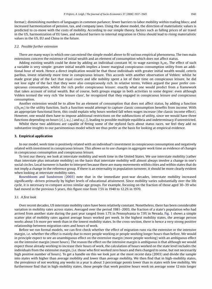
Over recent decades, US interstate mobility rates have been relatively constant. Nonetheless, there has been considerablevariation in mobility rates across states. Averaged over the period 1981–2003, the fraction of a state’s population who hadarrived from another state during the past year ranged from 1.7% in Pennsylvania to 7.9% in Nevada. Fig. 1 shows a simplescatter plot of mobility rates against average hours worked per week. In the highest mobility states, the average personworks about 5 h more per week than in the lowest mobility states. In the cross-section, there is hence a very strong positiverelationship between migration rates and hours of work.

Before we run formal models, we can first check whether the effect of migration runs via the extensive or the intensivemargin, i.e. whether the effect is mainly due to more people working or people working longer hours than before. We wouldin principle expect to see an unambiguous effect on the extensive margin (more people working) with an ambiguous effecton the intensive margin (more hours). The reason the effect on the intensive margin is ambiguous is that although we wouldexpect those already working to increase their hours of work, the calculation of hours worked on the state level includes theindividuals from the extensive margin, (i.e. those who first worked zero hours and then changed to some, but not necessarilyhigh positive number of hours). To get a handle on this we look just at the most recent data (2003) and divide the sampleinto states with higher than average mobility and lower than average mobility. We then find that in high-mobility states,the prevalence of not working any weeks in a year is about 3 percentage points lower than in states with low mobility. Wefurthermore find that in high-mobility states, those people that work positive hours work on average some 12 min longer


Fig. 1. Migration rate and hours worked, 1981–2003.

than individuals with positive hours in low mobility states. Both effects are statistically significant at the 1% level. Hence weseem to get movement both on the intensive margin and the extensive margin.

3.2. Extended analyses

The preliminary analyses above are not necessarily indicative of a causal effect of population turnover on conspicuousleisure because they ignore other factors that vary between states and over time. To test our theory in a more robust manner,we instead look for variation within states over time. We use the March supplement to the Current Population Surveyfrom 1981 to 2003, restricting our sample to those aged 16 and over. As our measure of mobility, we use a question thatasked whether the respondent had changed residence in the previous 12 months (i.e. since March 1 of the previous year).Respondents were coded as having moved if they had moved from another state. As our variation is only across state-yearcells, we can without loss of generality collapse the data to this level. This gives us 21 years of data, since the mobility questionwas not asked in 1985 and 1995. Across 50 states and the District of Columbia, the sample size is 1071.

Our dependent variables are three measures of labor supply: the usual number of hours worked per week in the previousyear; the number of weeks worked in the previous year; and the number of hours worked in the previous year (calculatedby multiplying together the first two numbers). The universe for all three variables is those who worked at some point inthe previous year. If conspicuous leisure is declining and conspicuous consumption is increasing, we should expect to see anincrease in labor supply. For those working full-time, this is more likely to occur on the hours margin, while for those witha weaker attachment to the labor force, it is more likely to occur on the weeks worked margin. One factor to bear in mind isthat if we only found an effect on weeks worked, we might worry that we were picking up a participation effect rather thana conspicuous leisure effect.

Naturally, many factors apart from population turnover could affect labor supply. We therefore present all our speci-fications with state and year fixed effects. In addition, we control for several demographic factors that might affect laborsupply: average age, average age squared, average years of education, fraction non-white, and fraction female. Furthermore,we include a set of controls intended to capture the effect of productivity shocks: the unemployment rate, the log of the pop-ulation size in the current and previous year, the log of the average hourly wage, and the log of the average personal incomeper capita. With the exception of the hourly wage, our productivity variables are not drawn from the CPS. Per capita personalincome is taken from the Bureau of Economic Analysis’s Annual State Personal Income series, while unemployment ratesand population figures are from the Bureau of Labor Statistics’ Local Area Unemployment figures. Note that by controllingfor both the log of the population size and the log of the population size in the previous year, our specification also implicitlyincludes the population growth rate (the difference between the two). Thus, if we find any significant population turnovereffects, they will not be driven by state growth, but rather by the amount of ‘population churn’ in a state, controlling for thestate’s size and growth rate.

Because the mobility question provides the average mobility rate from the previous March to the current March, while thelabor supply questions relate to the past calendar year (January to December), there is some question as to the appropriatelag structure. Clearly, labor supply decisions in January and February of the previous year cannot be affected by mobility inthe period from March onwards. Furthermore, there will probably be some lag between changes in mobility and changes inlabor supply. It may therefore be preferable to use the previous year’s mobility rate. Thus we present three specifications:

• the current period’s mobility rate, e.g. the effect of mobility from March 2002 to March 2003 on labor supply from January2002 to December 2002;


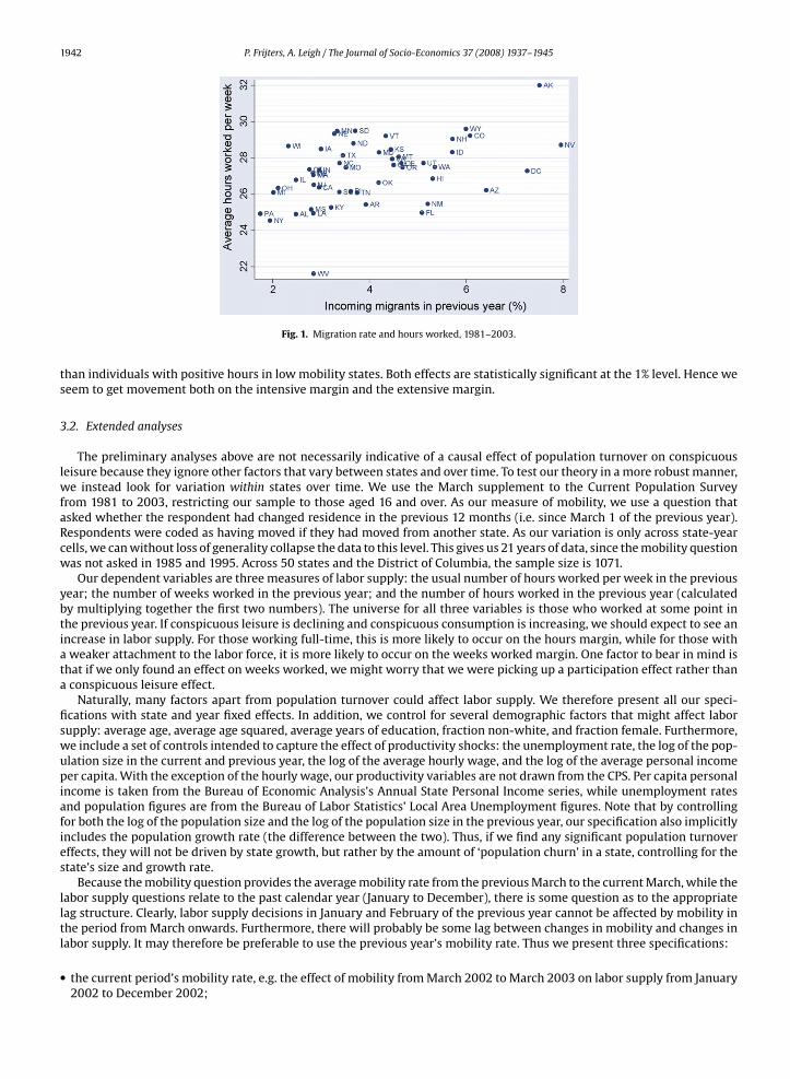
Table 1Summary statistics

Variable Mean S.D.

Migration rate 0.0401 0.017Hours per week 27.212 2.023Hours per week (excl migrants) 27.105 2.036Weeks per year 31.348 2.480Weeks per year (excl migrants) 31.424 2.501Hours per year 1248.739 107.418Hours per year (excl migrants) 1250.022 108.178Average age 42.921 1.637Fraction female 0.518 0.013Fraction non-white 0.145 0.138Average years of education 12.469 0.519Log personal income per capita 9.871 0.352Unemployment rate (percent) 6.000 2.147Log population 14.653 1.033Log average hourly wage 2.359 0.364

Sources: Labor supply, migration, age, gender, race, education and hourly wage from March CPS, 1981–2003 (excluding 1985 and 1995). Sample includes allrespondents aged 16 and over, collapsed to the state-year cell level. Specifications excluding migrants omit those who had moved into the state during theprevious 12 months. Unemployment rate and population figures from Bureau of Labor Statistics. Personal income from Bureau of Economic Analysis.

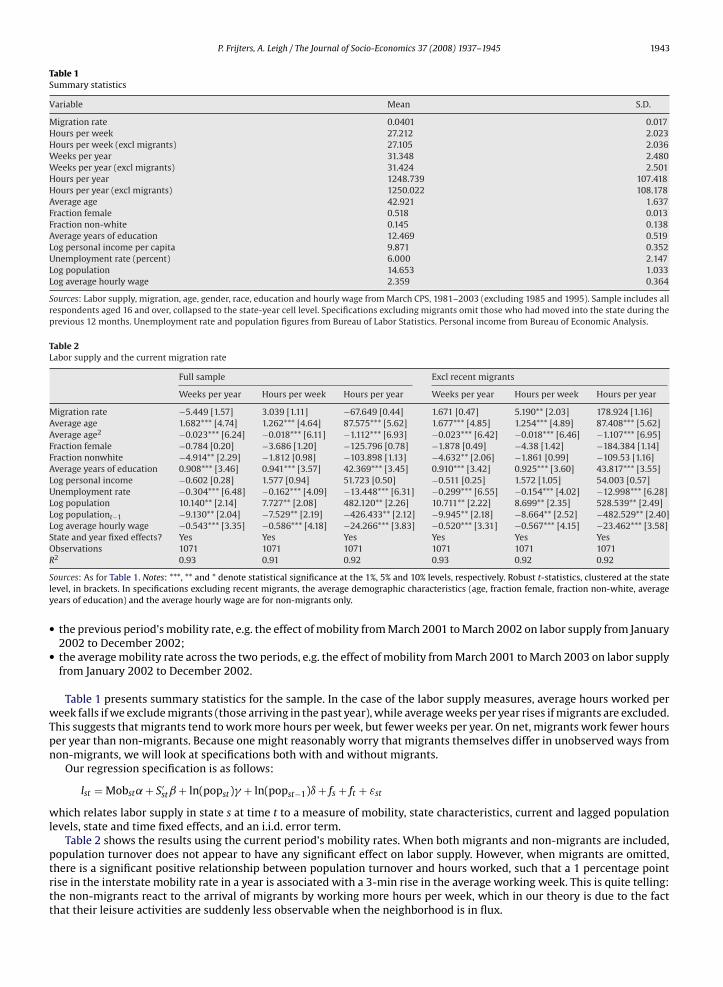
Table 2Labor supply and the current migration rate

Full sample Excl recent migrants

Weeks per year Hours per week Hours per year Weeks per year Hours per week Hours per year

Migration rate −5.449 [1.57] 3.039 [1.11] −67.649 [0.44] 1.671 [0.47] 5.190** [2.03] 178.924 [1.16]Average age 1.682*** [4.74] 1.262*** [4.64] 87.575*** [5.62] 1.677*** [4.85] 1.254*** [4.89] 87.408*** [5.62]Average age2 −0.023*** [6.24] −0.018*** [6.11] −1.112*** [6.93] −0.023*** [6.42] −0.018*** [6.46] −1.107*** [6.95]Fraction female −0.784 [0.20] −3.686 [1.20] −125.796 [0.78] −1.878 [0.49] −4.38 [1.42] −184.384 [1.14]Fraction nonwhite −4.914** [2.29] −1.812 [0.98] −103.898 [1.13] −4.632** [2.06] −1.861 [0.99] −109.53 [1.16]Average years of education 0.908*** [3.46] 0.941*** [3.57] 42.369*** [3.45] 0.910*** [3.42] 0.925*** [3.60] 43.817*** [3.55]Log personal income −0.602 [0.28] 1.577 [0.94] 51.723 [0.50] −0.511 [0.25] 1.572 [1.05] 54.003 [0.57]Unemployment rate −0.304*** [6.48] −0.162*** [4.09] −13.448*** [6.31] −0.299*** [6.55] −0.154*** [4.02] −12.998*** [6.28]Log population 10.140** [2.14] 7.727** [2.08] 482.120** [2.26] 10.711** [2.22] 8.699** [2.35] 528.539** [2.49]Log populationt−1 −9.130** [2.04] −7.529** [2.19] −426.433** [2.12] −9.945** [2.18] −8.664** [2.52] −482.529** [2.40]Log average hourly wage −0.543*** [3.35] −0.586*** [4.18] −24.266*** [3.83] −0.520*** [3.31] −0.567*** [4.15] −23.462*** [3.58]State and year fixed effects? Yes Yes Yes Yes Yes YesObservations 1071 1071 1071 1071 1071 1071R2 0.93 0.91 0.92 0.93 0.92 0.92

Sources: As for Table 1. Notes: ***, ** and * denote statistical significance at the 1%, 5% and 10% levels, respectively. Robust t-statistics, clustered at the statelevel, in brackets. In specifications excluding recent migrants, the average demographic characteristics (age, fraction female, fraction non-white, averageyears of education) and the average hourly wage are for non-migrants only.

• the previous period’s mobility rate, e.g. the effect of mobility from March 2001 to March 2002 on labor supply from January2002 to December 2002;

• the average mobility rate across the two periods, e.g. the effect of mobility from March 2001 to March 2003 on labor supplyfrom January 2002 to December 2002.

Table 1 presents summary statistics for the sample. In the case of the labor supply measures, average hours worked perweek falls if we exclude migrants (those arriving in the past year), while average weeks per year rises if migrants are excluded.This suggests that migrants tend to work more hours per week, but fewer weeks per year. On net, migrants work fewer hoursper year than non-migrants. Because one might reasonably worry that migrants themselves differ in unobserved ways fromnon-migrants, we will look at specifications both with and without migrants.

Our regression specification is as follows:

lst = Mobst˛ + S′stˇ + ln(popst)� + ln(popst−1)ı + fs + ft + εst

which relates labor supply in state s at time t to a measure of mobility, state characteristics, current and lagged populationlevels, state and time fixed effects, and an i.i.d. error term.

Table 2 shows the results using the current period’s mobility rates. When both migrants and non-migrants are included,population turnover does not appear to have any significant effect on labor supply. However, when migrants are omitted,there is a significant positive relationship between population turnover and hours worked, such that a 1 percentage pointrise in the interstate mobility rate in a year is associated with a 3-min rise in the average working week. This is quite telling:the non-migrants react to the arrival of migrants by working more hours per week, which in our theory is due to the factthat their leisure activities are suddenly less observable when the neighborhood is in flux.


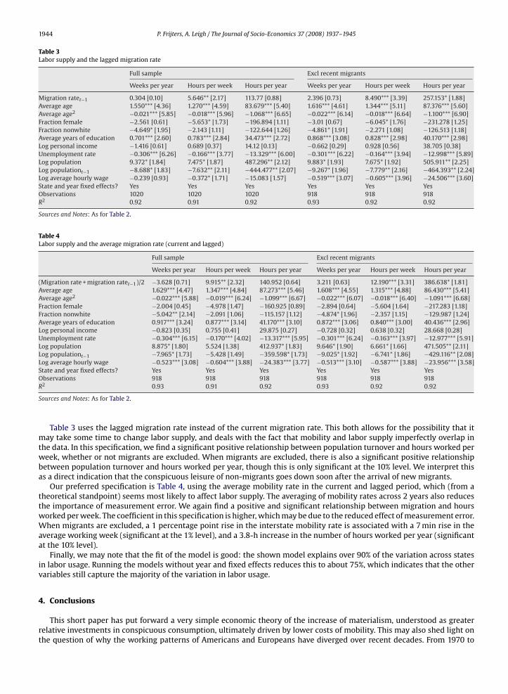
Table 3Labor supply and the lagged migration rate



Migration ratet−1 0.304 [0.10] 5.646** [2.17] 113.77 [0.88] 2.396 [0.73] 8.490*** [3.39] 257.153* [1.88]Average age 1.550*** [4.36] 1.270*** [4.59] 83.679*** [5.40] 1.616*** [4.61] 1.344*** [5.11] 87.376*** [5.60]Average age2 −0.021*** [5.85] −0.018*** [5.96] −1.068*** [6.65] −0.022*** [6.14] −0.018*** [6.64] −1.100*** [6.90]Fraction female −2.561 [0.61] −5.653* [1.73] −196.894 [1.11] −3.01 [0.67] −6.045* [1.76] −231.278 [1.25]Fraction nonwhite −4.649* [1.95] −2.143 [1.11] −122.644 [1.26] −4.861* [1.91] −2.271 [1.08] −126.513 [1.18]Average years of education 0.701*** [2.60] 0.783*** [2.84] 34.473*** [2.72] 0.868*** [3.08] 0.828*** [2.98] 40.170*** [2.98]Log personal income −1.416 [0.61] 0.689 [0.37] 14.12 [0.13] −0.662 [0.29] 0.928 [0.56] 38.705 [0.38]Unemployment rate −0.306*** [6.26] −0.166*** [3.77] −13.329*** [6.00] −0.301*** [6.22] −0.164*** [3.94] −12.998*** [5.89]Log population 9.372* [1.84] 7.475* [1.87] 487.296** [2.12] 9.883* [1.93] 7.675* [1.92] 505.911** [2.25]Log populationt−1 −8.688* [1.83] −7.632** [2.11] −444.477** [2.07] −9.267* [1.96] −7.779** [2.16] −464.393** [2.24]Log average hourly wage −0.239 [0.93] −0.372* [1.71] −15.083 [1.57] −0.519*** [3.07] −0.605*** [3.96] −24.506*** [3.60]State and year fixed effects? Yes Yes Yes Yes Yes YesObservations 1020 1020 1020 918 918 918R2 0.92 0.91 0.92 0.93 0.92 0.92

Sources and Notes: As for Table 2.

Table 4Labor supply and the average migration rate (current and lagged)



(Migration rate + migration ratet−1)/2 −3.628 [0.71] 9.915** [2.32] 140.952 [0.64] 3.211 [0.63] 12.190*** [3.31] 386.638* [1.81]Average age 1.629*** [4.47] 1.347*** [4.84] 87.273*** [5.46] 1.608*** [4.55] 1.315*** [4.88] 86.430*** [5.41]Average age2 −0.022*** [5.88] −0.019*** [6.24] −1.099*** [6.67] −0.022*** [6.07] −0.018*** [6.40] −1.091*** [6.68]Fraction female −2.004 [0.45] −4.978 [1.47] −160.925 [0.89] −2.894 [0.64] −5.604 [1.64] −217.283 [1.18]Fraction nonwhite −5.042** [2.14] −2.091 [1.06] −115.157 [1.12] −4.874* [1.96] −2.357 [1.15] −129.987 [1.24]Average years of education 0.917*** [3.24] 0.877*** [3.14] 41.170*** [3.10] 0.872*** [3.06] 0.840*** [3.00] 40.436*** [2.96]Log personal income −0.823 [0.35] 0.755 [0.41] 29.875 [0.27] −0.728 [0.32] 0.638 [0.32] 28.668 [0.28]Unemployment rate −0.304*** [6.15] −0.170*** [4.02] −13.317*** [5.95] −0.301*** [6.24] −0.163*** [3.97] −12.977*** [5.91]Log population 8.875* [1.80] 5.524 [1.38] 412.937* [1.83] 9.646* [1.90] 6.661* [1.66] 471.505** [2.11]Log populationt−1 −7.965* [1.73] −5.428 [1.49] −359.598* [1.73] −9.025* [1.92] −6.741* [1.86] −429.116** [2.08]Log average hourly wage −0.523*** [3.08] −0.604*** [3.88] −24.383*** [3.77] −0.513*** [3.10] −0.587*** [3.88] −23.956*** [3.58]State and year fixed effects? Yes Yes Yes Yes Yes YesObservations 918 918 918 918 918 918R2 0.93 0.91 0.92 0.93 0.92 0.92

Sources and Notes: As for Table 2.

Table 3 uses the lagged migration rate instead of the current migration rate. This both allows for the possibility that itmay take some time to change labor supply, and deals with the fact that mobility and labor supply imperfectly overlap inthe data. In this specification, we find a significant positive relationship between population turnover and hours worked perweek, whether or not migrants are excluded. When migrants are excluded, there is also a significant positive relationshipbetween population turnover and hours worked per year, though this is only significant at the 10% level. We interpret thisas a direct indication that the conspicuous leisure of non-migrants goes down soon after the arrival of new migrants.

Our preferred specification is Table 4, using the average mobility rate in the current and lagged period, which (from atheoretical standpoint) seems most likely to affect labor supply. The averaging of mobility rates across 2 years also reducesthe importance of measurement error. We again find a positive and significant relationship between migration and hoursworked per week. The coefficient in this specification is higher, which may be due to the reduced effect of measurement error.When migrants are excluded, a 1 percentage point rise in the interstate mobility rate is associated with a 7 min rise in theaverage working week (significant at the 1% level), and a 3.8-h increase in the number of hours worked per year (significantat the 10% level).

Finally, we may note that the fit of the model is good: the shown model explains over 90% of the variation across statesin labor usage. Running the models without year and fixed effects reduces this to about 75%, which indicates that the othervariables still capture the majority of the variation in labor usage.

4. Conclusions

This short paper has put forward a very simple economic theory of the increase of materialism, understood as greaterrelative investments in conspicuous consumption, ultimately driven by lower costs of mobility. This may also shed light onthe question of why the working patterns of Americans and Europeans have diverged over recent decades. From 1970 to


2002, the numbers of hours worked per year fell by 13 in the European Union, and grew by 20 in the US (OECD, 2004).6 Onepossible reason for this divergence could be that Europe has lower rates of internal migration than the US, largely due tolinguistic barriers between countries. High population turnover rates in the US might have helped to make Americans morematerialistic than Europeans. If policymakers wished to rectify this, the negative externality of mobility could in principlebe offset by a tax on mobility. However, such a tax would have other consequences, such as reducing the extent to whichpopulation mobility could act as a buffer against adverse regional shocks. Weighing these factors against one another isbeyond the scope of this paper.

There are many reasons to think that the increase in population turnover over recent years is on balance a positivedevelopment. In highly mobile societies such as the US, people can move from declining industrial cities to cities withbetter weather and amenities (Glaeser and Kohlhase, 2003), workers can relocate from high-unemployment regions tolow-unemployment regions, and citizens can choose neighborhoods with their preferred level of public goods provision(Tiebout, 1956).7 Yet it is nonetheless important to recognize that higher rates of population turnover impose a cost onothers, by requiring over-investment in conspicuous consumption, and under-investment in conspicuous leisure.

Taxes on mobility are institutionalized in many places, for instance in the form of real estate transfer taxes (known insome countries as ‘stamp duty’) on the purchase of a new house. Since mobility almost invariably is associated with thebuying and selling of a new house, the institution of stamp duty can be seen as a mobility tax. To the extent that the negativeexternality of mobility is not presently taken into account in setting real estate transfer tax rates, our paper provides anargument for increasing them.

An obvious alternative to taxing mobility is to directly tax goods that can be deemed to be conspicuous. This approachwould suggest that (to the extent that policymakers have not taken these factors into account), tax rates on luxury consump-tion goods should be higher than they are today.

Acknowledgements

We are grateful to seminar participants at the Australian National University and an anonymous referee for valuablecomments on earlier drafts. Susanne Schmidt provided outstanding research assistance.

References

Abel, A.B., 2005. Optimal taxation when consumers have endogenous benchmark levels of consumption. Review of Economic Studies 72, 21–42.Clark, A.E., Oswald, A.J., 1996. Satisfaction and comparison income. Journal of Public Economics 61, 359–381.Clark, A., Frijters, P., Shields, M.A., 2008. A survey of the income happiness gradient. Journal of Economic Literature 46 (March (1)), 95–144 (also IZA, NCER,

and DELTA discussion paper).Cushing-Daniels, B., 2004. Migration in the US: What Role Welfare? Mimeo, Gettysburg College, PA.Duesenberry, J.S., 1949. Income, Saving, and the Theory of Consumer Behavior. Harvard University Press, Cambridge, MA.Dupor, B., Liu, W.-F., 2003. Jealousy and equilibrium overconsumption. American Economic Review 93 (1), 423–428.Ferrer-i-Carbonel, A., Frijters, P., 2004. The effect of metholodogy on the determinants of happiness. Economic Journal 114, 641–659.Frank, R.H., 1985. The demand for unobservable and other positional goods. American Economic Review 71 (1), 101–116.Glaeser, E.L., Kohlhase, J.E., 2003. Cities, Regions and the Decline of Transport Costs, NBER Working Paper 9886, Cambridge, MA.Ireland, N.J., 1998. Status seeking, income taxation and efficiency. Journal of Public Economics 70, 99–113.Irving, G., 2007. Inequality and the Anglo-Saxon Economic Model, ICER 2007 Working Paper.Kinght, J., Song, L., 2004. Subjective Well-being and its Determinants in Rural China, Mimeo. University of Nottingham.Layard, R., 1980. Human satisfactions and public policy. Economic Journal 90 (363), 737–750.Layard, R., 2003. Happiness: has social science a clue? Lionel Robbins Memorial Lectures, London School of Economics (also forthcoming as a book).Ljungqvist, L., Uhlig, H., 2000. Tax policy and aggregate demand management under catching up with the Joneses. American Economic Review 90 (3),

356–366.Organisation for Economic Cooperation and Development, 2004. OECD Employment Outlook, OECD, Paris.Rosenbloom, J., Sundstrom, W., 2003. The Decline and Rise of Interstate Migration in the United States: Evidence From the IPUMS, 1850–1990, NBER Working

Paper 9857, Cambridge, MA.Samuelson, L., 2004. Information-based relative consumption effects. Econometrica 72 (1), 93–118.Stutzer, A., Lalive, R., 2004. The role of social work norms in job searching and subjective well-being. Journal of the European Economic Association 2 (4),

696–719.Tiebout, C., 1956. A pure theory of local expenditures. Journal of Political Economy 64, 416–424.Van de Stadt, H., Kapteyn, A., Van de Geer, S., 1985. The relativity of utility: evidence from panel data. The Review of Economics and Statistics 67, 179–187.Van Praag, B.M.S., 1977. The perception of welfare inequality. European Economic Review (10), 189–207.Veblen, T., 1898. The Theory of the Leisure Class. The Viking Press, New York.

6 This figure is the total number of hours divided by the total population, and thus captures both participation effects, and the hours worked by those inthe workforce. The figure for the European Union is for the EU-15 (excluding the 10 recent entrants).

7 Cushing-Daniels (2004) finds that while labor market differences have a significant impact on migration patterns, welfare generosity does not.

Documents

Materialism on the March: From conspicuous leisure to conspicuous consumption?