Material-Aware Mesh Deformationsmesh.brown.edu/DGP/pdfs/Popa-smi2006.pdf · Material-Aware Mesh Deformations ... Most real world objects consist of non-uniform materi-als; as a result,

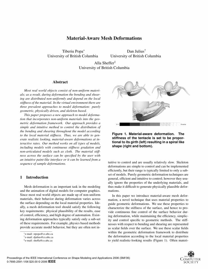
Material-Aware Mesh Deformations

Tiberiu Popa∗University of British Columbia

Dan Julius†

University of British Columbia

Alla Sheffer‡

University of British Columbia

Abstract

Most real world objects consist of non-uniform materi-als; as a result, during deformation the bending and shear-ing are distributed non-uniformly and depend on the localstiffness of the material. In the virtual environment there arethree prevalent approaches to model deformation: purelygeometric, physically driven, and skeleton based.

This paper proposes a new approach to model deforma-tion that incorporates non-uniform materials into the geo-metric deformation framework. Our approach provides asimple and intuitive method to control the distribution ofthe bending and shearing throughout the model accordingto the local material stiffness. Thus, we are able to gen-erate realistic looking, material-aware deformations at in-teractive rates. Our method works on all types of models,including models with continuous stiffness gradation andnon-articulated models such as cloth. The material stiff-ness across the surface can be specified by the user withan intuitive paint-like interface or it can be learned from asequence of sample deformations.

1 Introduction

Mesh deformation is an important task in the modeling

and the animation of digital models for computer graphics.

Since most real world objects are made up of non-uniform

materials, their behavior during deformation varies across

the surface depending on the local material properties. Ide-

ally, a mesh deformation tool should satisfy the following

key requirements: physical plausibility of the results, ease

of control, efficiency, and high degree of automation. Exist-

ing deformation approaches typically satisfy only a sub-set

of these requirements. For example, physics based methods

provide accurate model behavior, but they are often not in-

∗e-mail: [email protected]†e-mail: [email protected]‡e-mail: [email protected]

Figure 1. Material-aware deformation. Thestiffness of the tentacle is set to be propor-tional to its girth (left) resulting in a spiral likeshape (right and bottom).

tuitive to control and are usually relatively slow. Skeleton

deformations are simple to control and can be implemented

efficiently, but their range is typically limited to only a sub-

set of models. Purely geometric deformation techniques are

general, efficient and intuitive to control; however they usu-

ally ignore the properties of the underlying materials, and

thus make it difficult to generate physically plausible defor-

mations.

In this paper we introduce material-aware mesh defor-

mation, a novel technique that uses material properties to

guide geometric deformations. We use these properties to

characterize the stiffness of the surface, and hence to pro-

vide continuous fine control of the surface behavior dur-

ing deformation, while maintaining the efficiency, simplic-

ity and control specific to geometric methods. The stiff-

nesses with respect to bending and shearing are represented

as scalar fields over the surface. We use these scalar fields

within the geometric deformation framework to distribute

the deformation according to the local material properties

to yield realistic-looking results (Figure 1). Often materi-

Proceedings of the IEEE International Conference on Shape Modeling and Applications 2006 (SMI’06) 0-7695-2591-1/06 $20.00 © 2006 IEEE

als may exhibit anisotropic stiffness, for instance articulated

models often have joints with only one degree of freedom.

We support such anisotropic behavior by allowing three dif-

ferent scalar fields for the three orthogonal axes of rotation.

We are the first, to our knowledge, to support this feature.

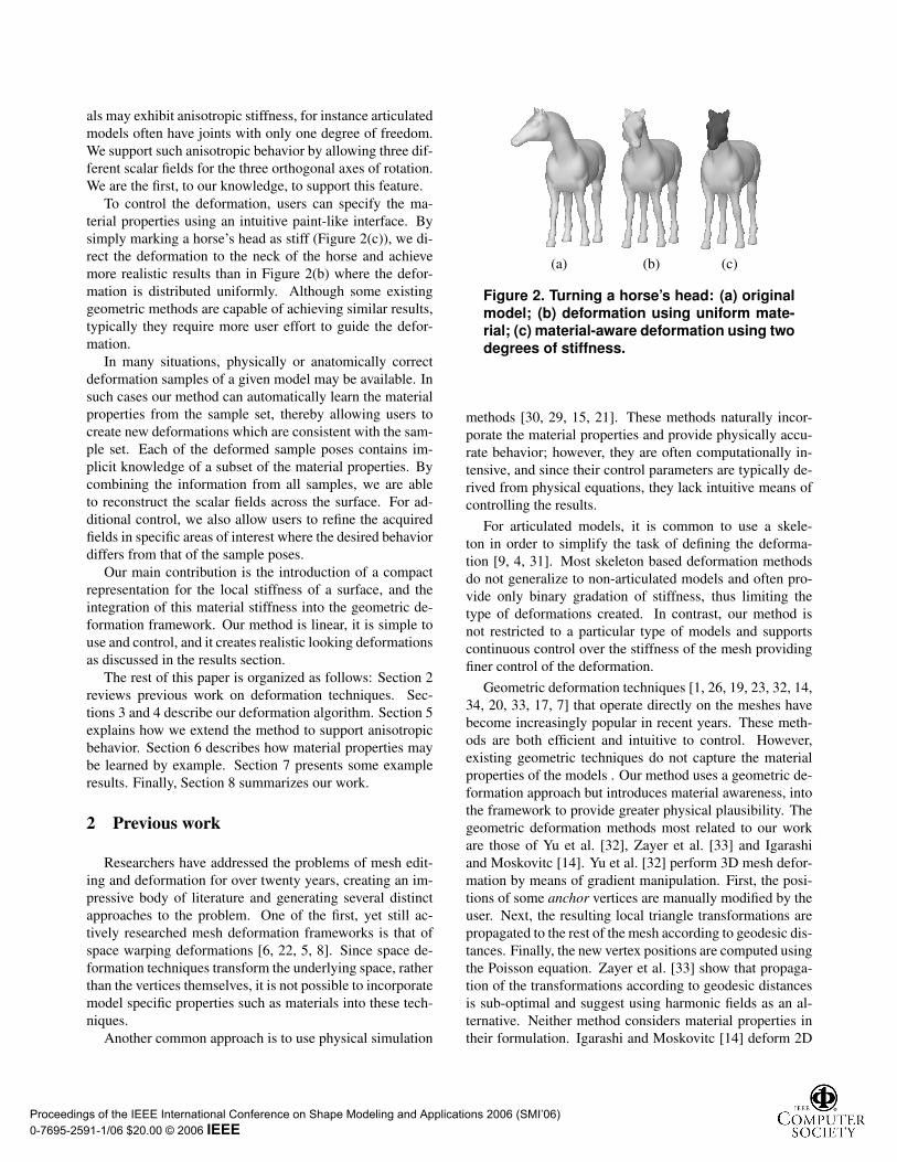
To control the deformation, users can specify the ma-

terial properties using an intuitive paint-like interface. By

simply marking a horse’s head as stiff (Figure 2(c)), we di-

rect the deformation to the neck of the horse and achieve

more realistic results than in Figure 2(b) where the defor-

mation is distributed uniformly. Although some existing

geometric methods are capable of achieving similar results,

typically they require more user effort to guide the defor-

mation.

In many situations, physically or anatomically correct

deformation samples of a given model may be available. In

such cases our method can automatically learn the material

properties from the sample set, thereby allowing users to

create new deformations which are consistent with the sam-

ple set. Each of the deformed sample poses contains im-

plicit knowledge of a subset of the material properties. By

combining the information from all samples, we are able

to reconstruct the scalar fields across the surface. For ad-

ditional control, we also allow users to refine the acquired

fields in specific areas of interest where the desired behavior

differs from that of the sample poses.

Our main contribution is the introduction of a compact

representation for the local stiffness of a surface, and the

integration of this material stiffness into the geometric de-

formation framework. Our method is linear, it is simple to

use and control, and it creates realistic looking deformations

as discussed in the results section.

The rest of this paper is organized as follows: Section 2

reviews previous work on deformation techniques. Sec-

tions 3 and 4 describe our deformation algorithm. Section 5

explains how we extend the method to support anisotropic

behavior. Section 6 describes how material properties may

be learned by example. Section 7 presents some example

results. Finally, Section 8 summarizes our work.

2 Previous work

Researchers have addressed the problems of mesh edit-

ing and deformation for over twenty years, creating an im-

pressive body of literature and generating several distinct

approaches to the problem. One of the first, yet still ac-

tively researched mesh deformation frameworks is that of

space warping deformations [6, 22, 5, 8]. Since space de-

formation techniques transform the underlying space, rather

than the vertices themselves, it is not possible to incorporate

model specific properties such as materials into these tech-

niques.

Another common approach is to use physical simulation

(a) (b) (c)

Figure 2. Turning a horse’s head: (a) originalmodel; (b) deformation using uniform mate-rial; (c) material-aware deformation using twodegrees of stiffness.

methods [30, 29, 15, 21]. These methods naturally incor-

porate the material properties and provide physically accu-

rate behavior; however, they are often computationally in-

tensive, and since their control parameters are typically de-

rived from physical equations, they lack intuitive means of

controlling the results.

For articulated models, it is common to use a skele-

ton in order to simplify the task of defining the deforma-

tion [9, 4, 31]. Most skeleton based deformation methods

do not generalize to non-articulated models and often pro-

vide only binary gradation of stiffness, thus limiting the

type of deformations created. In contrast, our method is

not restricted to a particular type of models and supports

continuous control over the stiffness of the mesh providing

finer control of the deformation.

Geometric deformation techniques [1, 26, 19, 23, 32, 14,

34, 20, 33, 17, 7] that operate directly on the meshes have

become increasingly popular in recent years. These meth-

ods are both efficient and intuitive to control. However,

existing geometric techniques do not capture the material

properties of the models . Our method uses a geometric de-

formation approach but introduces material awareness, into

the framework to provide greater physical plausibility. The

geometric deformation methods most related to our work

are those of Yu et al. [32], Zayer et al. [33] and Igarashi

and Moskovitc [14]. Yu et al. [32] perform 3D mesh defor-

mation by means of gradient manipulation. First, the posi-

tions of some anchor vertices are manually modified by the

user. Next, the resulting local triangle transformations are

propagated to the rest of the mesh according to geodesic dis-

tances. Finally, the new vertex positions are computed using

the Poisson equation. Zayer et al. [33] show that propaga-

tion of the transformations according to geodesic distances

is sub-optimal and suggest using harmonic fields as an al-

ternative. Neither method considers material properties in

their formulation. Igarashi and Moskovitc [14] deform 2D


Figure 3. Algorithm flow.

meshes using a formulation based on an earlier morphing

technique [3]. They manipulate the triangles independently

and then compute common vertex positions. They show

early research results for using material stiffness to control

the deformation. A direct extension of their method to 3D

would require a volumetric mesh, thus they acknowledge

that such an extension may be difficult.

It is often tedious and difficult to define the exact phys-

ical properties of an object. One alternative, presented by

two recent techniques [16, 28], is to create realistic-looking

deformations by mimicking existing physically correct ex-

ample deformations. James and Twigg [16] automatically

deduce the skeleton of an articulated model from a sam-

ple set of deformed models. Using the estimated skele-

ton and estimated blending weights they are able to create

new deformations consistent with the sample set. Sumner et

al. [28] use the set of sample models to create feature vec-

tors that span the space of meaningful deformations. Using

our method, we are able to use a set of sample poses as a

source for automatically learning the stiffness of the mesh.

The learned stiffness is used to create new poses consistent

with the samples. In our setting the material properties

are derived explicitly, therefore it is very easy for artists to

modify and refine those if desired.

3 Method overview

We present a two-step method for 3D mesh deformation

that takes into account the intrinsic material properties of

the model. To generate the deformation users select a small

set of triangles, called anchor triangles (Figure 3(a)) and

apply the desired transformations using a click and drag

motion. We support anchor transformations that include

any combination of rotations and uniform scales. We then

calculate transformations for the remaining triangles of the

mesh based on the anchor transformations. The calcula-

tion takes into account the material properties of the model

which are described as follows.

Material properties — To describe the impact of the

material on the deformation we define the stiffness of the

material with respect to bending and shearing. These stiff-

nesses are described by separate scalar fields defined across

the mesh. Since materials often bend differently with re-

spect to different directions, we also allow users to define

anisotropic bending stiffness fields. The user can define

these scalar fields using a paintbrush-like tool (Figure 3(b)).

We also introduce a data-driven approach for defining

the stiffnesses by automatically learning them from a set

of example deformations (Figure 3(c)). By examining the

shearing of each individual triangle and the difference in

the transformations undergone by adjacent triangles within

the entire sample set, we are able to identify degrees of stiff-

ness and flexibility across the mesh, and thus reconstruct the

stiffness fields (Figure 3(d)).

Next, we explain how these stiffness scalar fields, to-

gether with the user defined transformations at anchor tri-

angles, are used in our algorithm.

Transformation extrapolation — The first step of

the algorithm is to propagate automatically the transforma-

tions from the anchors to the remaining triangles in the

mesh. Finding optimal transformations for each triangle

is non-trivial since these must comply with a number of

constraints. First, the transformations must be continuous

across the surface to yield a smooth looking deformation.

Next, the transformations must also be as-rigid-as-possible

in order to maintain the details of the original surface [32].

Finally, in our setting we add one new constraint — the

transformations must be consistent with the material prop-

erties. This final requirement is the one that ensures our

deformations behave as desired.

We suggest that each triangle transformation be a

weighted sum, or blend, of anchor transformations. Thus,

our challenge is to find appropriate weights for blending that

comply with the previous requirements. We formulate this

as a linear optimization problem where the variables are the

blending weights. The stiffness fields are introduced into

the formulation to ensure that the deformation is distributed

correctly throughout the model. Since the solution depends

only on the selection of anchors, we need to solve the result-

ing system only once. To perform the actual blending we

use the transformation algebra defined by Alexa [2]. For a

discussions on the optimality of this method, see Appendix

A

Vertex repositioning — It is easy to see that apply-


ing the resulting transformations to each of the triangles in

the mesh independently will break the mesh connectivity,

since adjacent triangles are not necessarily assigned iden-

tical transformations (Figure 3(e)). Therefore we apply a

second step in which we calculate optimal vertex positions

such that each triangle is transformed as closely as possi-

ble, in the least squares sense, to the previously calculated

transformations (Figure 3(f)). We incorporate the shearing

stiffness field into the formulation to ensure that most of the

resulting shearing is concentrated in the flexible areas of the

mesh.

Figure 3 summarizes our algorithm, and the following

three sections describe it in detail: Section 4 explains how

transformations are propagated and then optimal vertex po-

sitions are found, Section 5 explains how the method is ex-

tended to support anisotropic stiffnesses, and Section 6 ex-

plains how the material stiffnesses are estimated from sam-

ple deformations.

4 Method details

We begin this section by describing exactly how our ma-

terial properties are defined (Section 4.1). Next, we de-

fine the gradient transformations and explain how these are

propagated from anchor triangles (Section 4.2). Finally,

we explain how optimal vertex positions are found (Sec-

tion 4.3).

4.1 Material properties

We formulate our material properties in terms of ma-

terial resistance to bending and shearing. This resistance

is described by bending and shearing stiffness scalar fields

defined across the mesh. This approach allows a high de-

gree of control with smooth variations of stiffness across

the mesh.

• The bending stiffness is associated with the mesh

edges, reflecting the bending flexibility of each edge.

Thus the bending scalar field is defined by a set of val-

ues ϕi j defined on the mesh edges (i, j). This field

is used to propagate the anchor transformations across

the mesh (Equation 1).

• The shearing stiffness is associated with the mesh faces

reflecting the resistance to shearing of each individual

face. The shearing stiffnesses ψi defined for the mesh

faces are used to find optimal vertex positions (Equa-

tion 3).

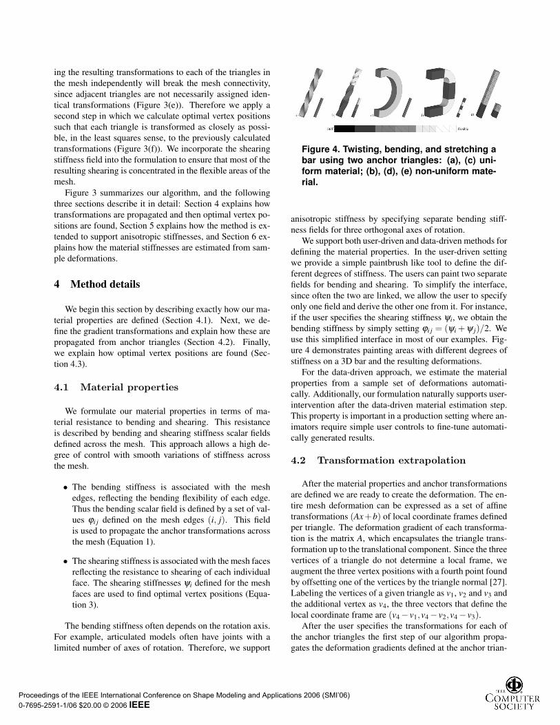
The bending stiffness often depends on the rotation axis.

For example, articulated models often have joints with a

limited number of axes of rotation. Therefore, we support

Figure 4. Twisting, bending, and stretching abar using two anchor triangles: (a), (c) uni-form material; (b), (d), (e) non-uniform mate-rial.

anisotropic stiffness by specifying separate bending stiff-

ness fields for three orthogonal axes of rotation.

We support both user-driven and data-driven methods for

defining the material properties. In the user-driven setting

we provide a simple paintbrush like tool to define the dif-

ferent degrees of stiffness. The users can paint two separate

fields for bending and shearing. To simplify the interface,

since often the two are linked, we allow the user to specify

only one field and derive the other one from it. For instance,

if the user specifies the shearing stiffness ψi, we obtain the

bending stiffness by simply setting ϕi j = (ψi + ψ j)/2. We

use this simplified interface in most of our examples. Fig-

ure 4 demonstrates painting areas with different degrees of

stiffness on a 3D bar and the resulting deformations.

For the data-driven approach, we estimate the material

properties from a sample set of deformations automati-

cally. Additionally, our formulation naturally supports user-

intervention after the data-driven material estimation step.

This property is important in a production setting where an-

imators require simple user controls to fine-tune automati-

cally generated results.

4.2 Transformation extrapolation

After the material properties and anchor transformations

are defined we are ready to create the deformation. The en-

tire mesh deformation can be expressed as a set of affine

transformations (Ax+b) of local coordinate frames defined

per triangle. The deformation gradient of each transforma-

tion is the matrix A, which encapsulates the triangle trans-

formation up to the translational component. Since the three

vertices of a triangle do not determine a local frame, we

augment the three vertex positions with a fourth point found

by offsetting one of the vertices by the triangle normal [27].

Labeling the vertices of a given triangle as v1, v2 and v3 and

the additional vertex as v4, the three vectors that define the

local coordinate frame are (v4 − v1,v4 − v2,v4 − v3).After the user specifies the transformations for each of

the anchor triangles the first step of our algorithm propa-

gates the deformation gradients defined at the anchor trian-


gles to the remaining triangles of the mesh. We achieve this

by using a weighted blending of anchor transformations.

As previously noted, our challenge is to find appropriate

weights for this blending, subject to the material properties.

In our setting, this implies that triangles in areas which are

more resistant to bending should be assigned more similar

transformations. In the isotropic setting, we formulate this

as a linear optimization problem:

minωi∈Rk

∑(i, j)∈E

ϕi j ‖ ωi −ω j ‖22, (1)

where the unknowns are ωi ∈ Rk the blending weights for

face i. Each ωi is a vector (ω1i ,ω2

i , . . . ,ωki ) where ωa

i de-

notes the relative influence of anchor transformation a. k is

the number of anchor triangles, E is the set of edges (ex-

cluding edges shared by two anchor triangles and boundary

edges) and ϕi j are the bending stiffness values associated

with each edge. The anisotropic setting is slightly different,

and is explained in Section 5.

When ϕi j is large, ωi and ω j will have similar values;

thus, the resulting transformations of the two adjacent tri-

angles i and j will also be similar, and the mesh may be

considered as locally stiff. Similarly, the converse argument

can be made for small ϕi j.

Note that in this formulation, the weights ωi depend only

on the connectivity of the mesh and on the selection of an-

chor triangles. Therefore, the weights need to be computed

only once per selection of anchors. Also, note that, since

our anchor coefficients have exactly one non-zero entry, our

weights are barycentric coordinates with respect to the an-

chors. As a result our method does not suffer from propaga-

tion problems noted by Zayer [33] encountered when using

weights based on geodesic distances [32]. This formula-

tion resembles that of [33], however in our formulation we

added non-uniform stiffness support.

In order to perform the actual blending we use the

commutative transformation matrix algebra defined by

Alexa [2]. By defining two new operations denoted by ⊕and �, the blended transformations Ti with weights ω i are

computed as:

Ti =k⊕

a=1

ωai �Ta. (2)

Details on these operators are found in Appendix A. Fig-

ure 3(e) illustrates the propagated transformations between

two anchors on the camel’s leg.

4.3 Vertex repositioning

Since the transformations obtained for adjacent triangles

are typically not identical, applying each of the transforma-

tions as-is would result in ambiguous positions for the two

shared vertices. Therefore, we need a second stage to com-

pute the optimal position for each vertex.

Optimal vertex positions are found such that the gradient

transformation of each triangle remains as close as possi-

ble, in the least squares sense, to the previously calculated

transformation [27]. Since the process results in triangle

shearing, we introduce the shearing stiffness into the for-

mulation, to direct the distortion according to the flexibility

of the mesh.

Sumner and Popovic [27] show that the transformation

gradients can be expressed in terms of the vertex positions

before and after the deformation:

A = VV−1,

where

V = (v4 − v1, v4 − v2, v4 − v3) ,

V = (v4 − v1,v4 − v2,v4 − v3) ,

and vi is the position of vertex vi after applying the deforma-

tion transformation. Next, the system is reformulated such

that the unknowns are the new vertex positions v.

The optimal solution is obtained when the resulting tri-

angle transformations are as close as possible to the previ-

ously computed Ti’s. Since the Ti’s are blends of the origi-

nal anchor transformations, they contain no shearing. Thus,

the closer the final and the original transformations are, the

smaller the triangle shearing. To account for the shearing

stiffness we incorporated ψi into the formulation:

minv

n−k

∑i

ψi‖ViV−1i −Ti‖2

F , (3)

where Vi and Vi are the local frames before and after ap-

plying the deformation and Ti are the previously calculated

transformations. We reformulate this as a linear optimiza-

tion problem:

minv

‖Ψ(Av− t)‖22, (4)

where A is a sparse matrix constructed using the pre-

deformation local frames V , t is a vector composed of all

the elements in Ti and Ψ is a diagonal matrix composed of

ψi.

Large ψi will result in transformations which are very

close to the originally computed Ti, and thus exhibit less

shearing. Small ψi will allow for more shearing to take

place. Figure 4(e) shows an example of stretching a bar

with non-uniform shearing stiffness. As expected, most of

the shearing occurs in the flexible region.

The solution of the system in Equation 4 provides a new

position for each of the vertices up to a global translation of

the model. To anchor the model in place, we fix the position

of a single vertex by removing the corresponding variable

and pre-multiplying its known position with the appropri-

ate elements of A into the vector T [28]. In fact, multiple


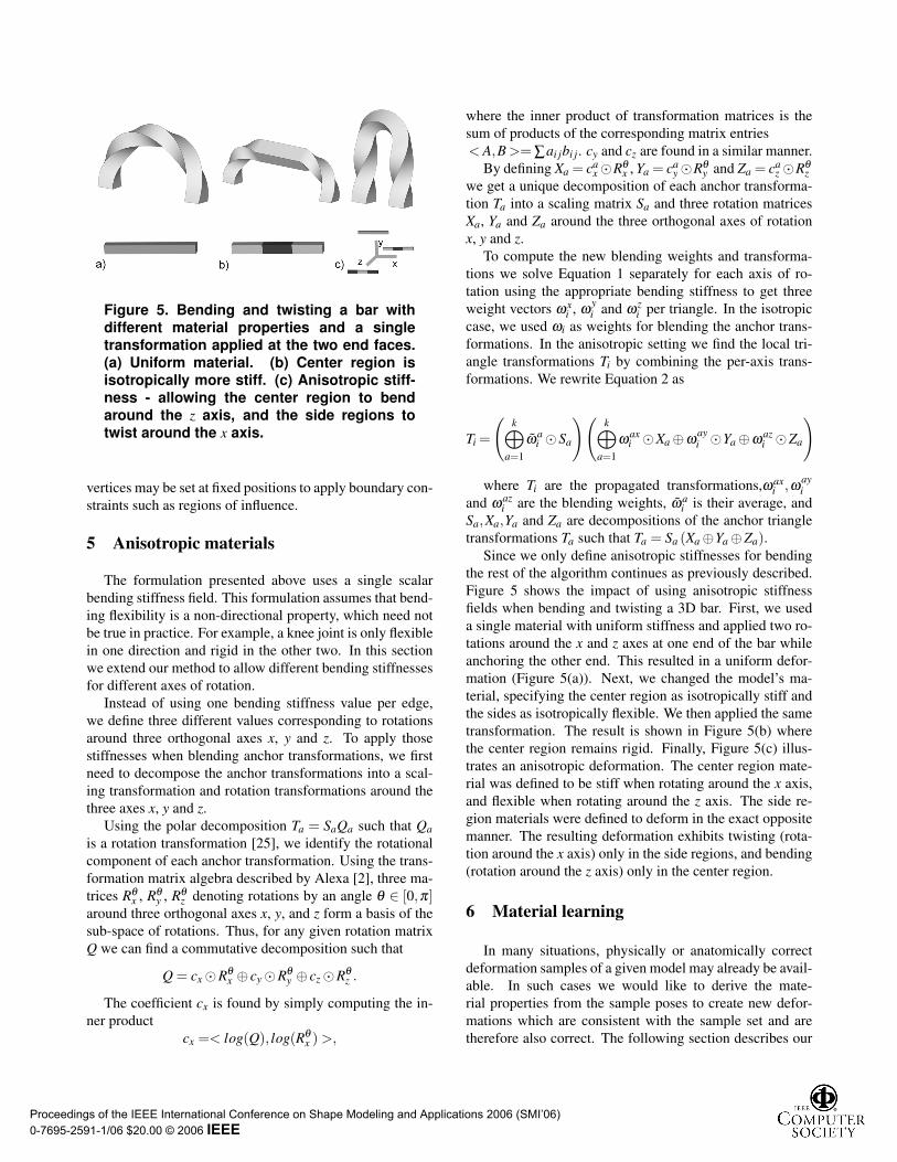
Figure 5. Bending and twisting a bar withdifferent material properties and a singletransformation applied at the two end faces.(a) Uniform material. (b) Center region isisotropically more stiff. (c) Anisotropic stiff-ness - allowing the center region to bendaround the z axis, and the side regions totwist around the x axis.

vertices may be set at fixed positions to apply boundary con-

straints such as regions of influence.

5 Anisotropic materials

The formulation presented above uses a single scalar

bending stiffness field. This formulation assumes that bend-

ing flexibility is a non-directional property, which need not

be true in practice. For example, a knee joint is only flexible

in one direction and rigid in the other two. In this section

we extend our method to allow different bending stiffnesses

for different axes of rotation.

Instead of using one bending stiffness value per edge,

we define three different values corresponding to rotations

around three orthogonal axes x, y and z. To apply those

stiffnesses when blending anchor transformations, we first

need to decompose the anchor transformations into a scal-

ing transformation and rotation transformations around the

three axes x, y and z.

Using the polar decomposition Ta = SaQa such that Qais a rotation transformation [25], we identify the rotational

component of each anchor transformation. Using the trans-

formation matrix algebra described by Alexa [2], three ma-

trices Rθx , Rθ

y , Rθz denoting rotations by an angle θ ∈ [0,π]

around three orthogonal axes x, y, and z form a basis of the

sub-space of rotations. Thus, for any given rotation matrix

Q we can find a commutative decomposition such that

Q = cx �Rθx ⊕ cy �Rθ

y ⊕ cz �Rθz .

The coefficient cx is found by simply computing the in-

ner product

cx =< log(Q), log(Rθx ) >,

where the inner product of transformation matrices is the

sum of products of the corresponding matrix entries

< A,B >= ∑ai jbi j. cy and cz are found in a similar manner.

By defining Xa = cax �Rθ

x , Ya = cay �Rθ

y and Za = caz �Rθ

zwe get a unique decomposition of each anchor transforma-

tion Ta into a scaling matrix Sa and three rotation matrices

Xa, Ya and Za around the three orthogonal axes of rotation

x, y and z.

To compute the new blending weights and transforma-

tions we solve Equation 1 separately for each axis of ro-

tation using the appropriate bending stiffness to get three

weight vectors ωxi , ωy

i and ωzi per triangle. In the isotropic

case, we used ωi as weights for blending the anchor trans-

formations. In the anisotropic setting we find the local tri-

angle transformations Ti by combining the per-axis trans-

formations. We rewrite Equation 2 as

Ti =

(k⊕

a=1

ωai �Sa

)(k⊕

a=1

ωaxi �Xa ⊕ωay

i �Ya ⊕ωazi �Za

)

where Ti are the propagated transformations,ωaxi ,ωay

iand ωaz

i are the blending weights, ωai is their average, and

Sa,Xa,Ya and Za are decompositions of the anchor triangle

transformations Ta such that Ta = Sa (Xa ⊕Ya ⊕Za).Since we only define anisotropic stiffnesses for bending

the rest of the algorithm continues as previously described.

Figure 5 shows the impact of using anisotropic stiffness

fields when bending and twisting a 3D bar. First, we used

a single material with uniform stiffness and applied two ro-

tations around the x and z axes at one end of the bar while

anchoring the other end. This resulted in a uniform defor-

mation (Figure 5(a)). Next, we changed the model’s ma-

terial, specifying the center region as isotropically stiff and

the sides as isotropically flexible. We then applied the same

transformation. The result is shown in Figure 5(b) where

the center region remains rigid. Finally, Figure 5(c) illus-

trates an anisotropic deformation. The center region mate-

rial was defined to be stiff when rotating around the x axis,

and flexible when rotating around the z axis. The side re-

gion materials were defined to deform in the exact opposite

manner. The resulting deformation exhibits twisting (rota-

tion around the x axis) only in the side regions, and bending

(rotation around the z axis) only in the center region.

6 Material learning

In many situations, physically or anatomically correct

deformation samples of a given model may already be avail-

able. In such cases we would like to derive the mate-

rial properties from the sample poses to create new defor-

mations which are consistent with the sample set and are

therefore also correct. The following section describes our


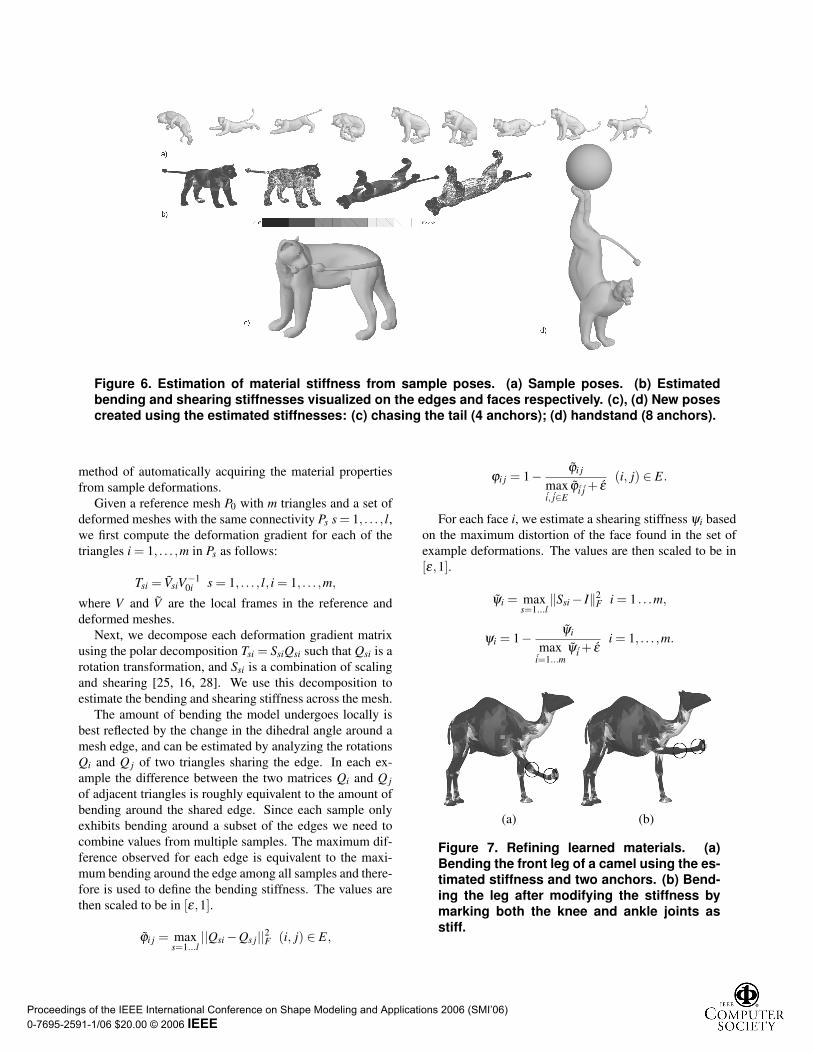
Figure 6. Estimation of material stiffness from sample poses. (a) Sample poses. (b) Estimatedbending and shearing stiffnesses visualized on the edges and faces respectively. (c), (d) New posescreated using the estimated stiffnesses: (c) chasing the tail (4 anchors); (d) handstand (8 anchors).

method of automatically acquiring the material properties

from sample deformations.

Given a reference mesh P0 with m triangles and a set of

deformed meshes with the same connectivity Ps s = 1, . . . , l,we first compute the deformation gradient for each of the

triangles i = 1, . . . ,m in Ps as follows:

Tsi = VsiV−10i s = 1, . . . , l, i = 1, . . . ,m,

where V and V are the local frames in the reference and

deformed meshes.

Next, we decompose each deformation gradient matrix

using the polar decomposition Tsi = SsiQsi such that Qsi is a

rotation transformation, and Ssi is a combination of scaling

and shearing [25, 16, 28]. We use this decomposition to

estimate the bending and shearing stiffness across the mesh.

The amount of bending the model undergoes locally is

best reflected by the change in the dihedral angle around a

mesh edge, and can be estimated by analyzing the rotations

Qi and Q j of two triangles sharing the edge. In each ex-

ample the difference between the two matrices Qi and Q jof adjacent triangles is roughly equivalent to the amount of

bending around the shared edge. Since each sample only

exhibits bending around a subset of the edges we need to

combine values from multiple samples. The maximum dif-

ference observed for each edge is equivalent to the maxi-

mum bending around the edge among all samples and there-

fore is used to define the bending stiffness. The values are

then scaled to be in [ε,1].

ϕi j = maxs=1...l

||Qsi −Qs j||2F (i, j) ∈ E,

ϕi j = 1− ϕi j

maxi, j∈E

ϕi j + ε(i, j) ∈ E.

For each face i, we estimate a shearing stiffness ψi based

on the maximum distortion of the face found in the set of

example deformations. The values are then scaled to be in

[ε,1].

ψi = maxs=1...l

‖Ssi − I‖2F i = 1 . . .m,

ψi = 1− ψi

maxi=1...m

ψi + εi = 1, . . . ,m.

(a) (b)

Figure 7. Refining learned materials. (a)Bending the front leg of a camel using the es-timated stiffness and two anchors. (b) Bend-ing the leg after modifying the stiffness bymarking both the knee and ankle joints asstiff.


Figure 8. Deformation of articulated models using our technique: (a), (c) original models and paintedstiffnesses; (b), (d) deformation results.

For both scalar fields we found that clamping the bottom

1% of the values before scaling greatly improved the results.

Figure 6 shows an example of estimated bending and

shearing stiffnesses learned from a sample sequence of de-

formations. As shown in the figure we use these as a basis

for creating new poses which were not in the sample set.

Our method is much simpler than those of James and

Twigg [16] and Sumner et al. [28], who also use polar de-

composition as the first step in their methods. However,

some problems can occur when stiffness coefficients of dif-

ferent parts of the body are learned independently from dif-

ferent poses. In these cases there is no information on the

relative stiffness between these parts and hence the relative

scale of the stiffness coefficients may not be correct. Nev-

ertheless, our experimental results appear to correctly cap-

ture the model’s material properties, and to provide realistic

looking deformations. Furthermore, our method exhibits

two nice properties: our learning algorithm is linear in the

number of sample poses, and the learned stiffnesses can be

further refined by the user for finer control.

7 Implementation and results

We now provide some implementational details and dis-

cuss some deformations created by our technique. We used

Graphite [12] as a framework for implementing our defor-

mation method. Material properties are defined using a sim-

ple color map with a paintbrush interface. To deform mod-

els users mark anchor triangles and then transform them by

dragging the mouse. Note that in all our examples except

Figure 4(e) we defined only the rotation and scaling for the

anchor triangles without fixing their final positions. We let

the algorithm find these optimal positions automatically.

We used the UMFPACK4.4 [10] solver to compute the

solutions of equations 1 and 4. In each of the equations the

required matrix inversion depends only on the selection of

anchor triangles, the mesh connectivity, and the undeformed

mesh geometry. We can therefore precompute the inverse

of these matrices, allowing the system to work at interactive

rates.

We support the concept of deforming only regions of in-

terest, confining all the calculations to triangles within that

region. When using such a region of interest, the vertices

on its boundary are constrained to remain in their initial po-

sition. Our results demonstrate that the method may be ap-

plied to a large variety of model types.

Figure 9. Scaling and rotating a camel’shead. Top: uniform material causes the en-tire camel to scale and rotate. Bottom: thestiff head scales uniformly, while the flexibleneck absorbs the distortion.


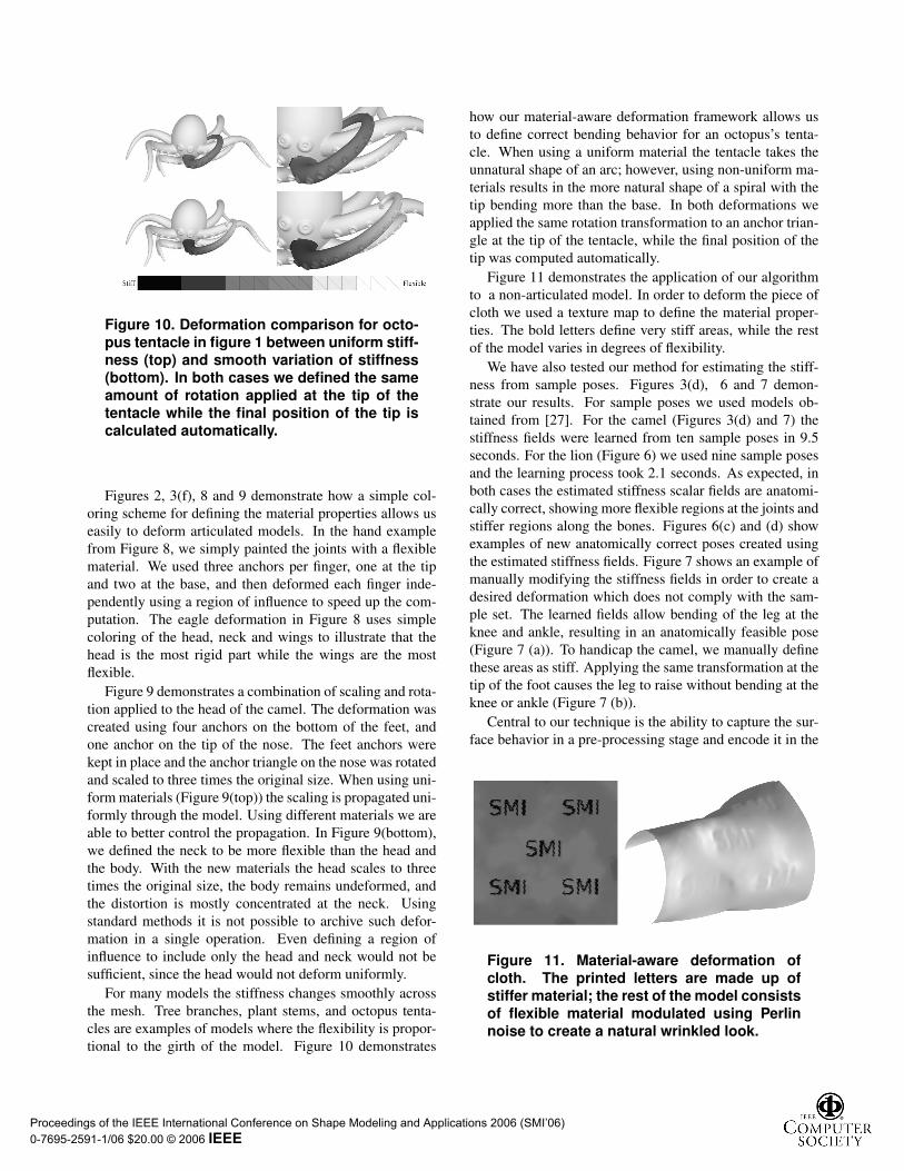
Figure 10. Deformation comparison for octo-pus tentacle in figure 1 between uniform stiff-ness (top) and smooth variation of stiffness(bottom). In both cases we defined the sameamount of rotation applied at the tip of thetentacle while the final position of the tip iscalculated automatically.

Figures 2, 3(f), 8 and 9 demonstrate how a simple col-

oring scheme for defining the material properties allows us

easily to deform articulated models. In the hand example

from Figure 8, we simply painted the joints with a flexible

material. We used three anchors per finger, one at the tip

and two at the base, and then deformed each finger inde-

pendently using a region of influence to speed up the com-

putation. The eagle deformation in Figure 8 uses simple

coloring of the head, neck and wings to illustrate that the

head is the most rigid part while the wings are the most

flexible.

Figure 9 demonstrates a combination of scaling and rota-

tion applied to the head of the camel. The deformation was

created using four anchors on the bottom of the feet, and

one anchor on the tip of the nose. The feet anchors were

kept in place and the anchor triangle on the nose was rotated

and scaled to three times the original size. When using uni-

form materials (Figure 9(top)) the scaling is propagated uni-

formly through the model. Using different materials we are

able to better control the propagation. In Figure 9(bottom),

we defined the neck to be more flexible than the head and

the body. With the new materials the head scales to three

times the original size, the body remains undeformed, and

the distortion is mostly concentrated at the neck. Using

standard methods it is not possible to archive such defor-

mation in a single operation. Even defining a region of

influence to include only the head and neck would not be

sufficient, since the head would not deform uniformly.

For many models the stiffness changes smoothly across

the mesh. Tree branches, plant stems, and octopus tenta-

cles are examples of models where the flexibility is propor-

tional to the girth of the model. Figure 10 demonstrates

how our material-aware deformation framework allows us

to define correct bending behavior for an octopus’s tenta-

cle. When using a uniform material the tentacle takes the

unnatural shape of an arc; however, using non-uniform ma-

terials results in the more natural shape of a spiral with the

tip bending more than the base. In both deformations we

applied the same rotation transformation to an anchor trian-

gle at the tip of the tentacle, while the final position of the

tip was computed automatically.

Figure 11 demonstrates the application of our algorithm

to a non-articulated model. In order to deform the piece of

cloth we used a texture map to define the material proper-

ties. The bold letters define very stiff areas, while the rest

of the model varies in degrees of flexibility.

We have also tested our method for estimating the stiff-

ness from sample poses. Figures 3(d), 6 and 7 demon-

strate our results. For sample poses we used models ob-

tained from [27]. For the camel (Figures 3(d) and 7) the

stiffness fields were learned from ten sample poses in 9.5

seconds. For the lion (Figure 6) we used nine sample poses

and the learning process took 2.1 seconds. As expected, in

both cases the estimated stiffness scalar fields are anatomi-

cally correct, showing more flexible regions at the joints and

stiffer regions along the bones. Figures 6(c) and (d) show

examples of new anatomically correct poses created using

the estimated stiffness fields. Figure 7 shows an example of

manually modifying the stiffness fields in order to create a

desired deformation which does not comply with the sam-

ple set. The learned fields allow bending of the leg at the

knee and ankle, resulting in an anatomically feasible pose

(Figure 7 (a)). To handicap the camel, we manually define

these areas as stiff. Applying the same transformation at the

tip of the foot causes the leg to raise without bending at the

knee or ankle (Figure 7 (b)).

Central to our technique is the ability to capture the sur-

face behavior in a pre-processing stage and encode it in the

Figure 11. Material-aware deformation ofcloth. The printed letters are made up ofstiffer material; the rest of the model consistsof flexible material modulated using Perlinnoise to create a natural wrinkled look.


formulation. We successfully capture the material proper-

ties while preserving the simplicity and efficiency common

to geometric deformation techniques. We demonstrated that

our technique can be applied to a wide range of models pro-

ducing complex results with only few anchors.

Table 1 summarizes the deformation statistics of the var-

ious models used in our results, measured on a 3GHz Intel

Pentium IV with 2Gb of RAM.

8 Summary and future work

We presented a new mesh deformation technique that

incorporates material properties into the geometric defor-

mation framework. Using these properties, we provide a

simple mechanism that allows material-aware behavior of

the surface under deformation. Our method combines the

efficiency, generality and control of geometric methods to-

gether with material awareness found in physical and skele-

ton based methods.

Material properties can be user-driven, where the stiff-

nesses are specified with a simple brush-like interface, or

data-driven where stiffnesses are deduced from a set of

given poses. It also can be a combination of the two where

the user can override the learned material stiffnesses.

The formulation is simple and efficient. It requires solv-

ing only two linear systems, and thus works at interactive

rates. The resulting deformations are as-rigid-as-possible,

subject to the material stiffness and the user defined trans-

formations, and therefore maintain the shape details as

demonstrated in our results.

For future research we would like to improve the

anisotropic model. The current anisotropic model uses a

global coordinate frame to decompose local rotations in-

stead of local coordinate frames. Decomposition around lo-

cal coordinate frames would be preferred because the stiff-

ness maps would be invariant to the position and orientation

of an object in space. However, the challenge in doing so is

the consistent construction of blending weights across dif-

ferent coordinate frames.

9 Acknowledgments

We would like to thank Ciaran Llachlan Leavitt for help

with editing the paper. We would like to thank Robert

Sumner for the lion and camel models and ETH Zurich for

the octopus model. This project was partially funded by

NSERC.

References

[1] M. Alexa. Local control for mesh morphing. In SMI ’01:Proceedings of the International Conference on Shape Mod-

eling & Applications, page 209, Washington, DC, USA,

2001. IEEE Computer Society.[2] M. Alexa. Linear combination of transformations. In SIG-

GRAPH ’02: Proceedings of the 29th annual conference onComputer graphics and interactive techniques, pages 380–

387, New York, NY, USA, 2002. ACM Press.[3] M. Alexa, D. Cohen-Or, and D. Levin. As-rigid-as-possible

shape interpolation. In K. Akeley, editor, Siggraph 2000,Computer Graphics Proceedings, pages 157–164. ACM

Press / ACM SIGGRAPH / Addison Wesley Longman,

2000.[4] B. Allen, B. Curless, and Z. Popovic. Articulated body de-

formation from range scan data. 21(3):612–619, 2002.[5] A. Angelidis, M.-P. Cani, G. Wyvill, and S. A. King.

Swirling-sweepers: Constant-volume modeling. In PacificConference on Computer Graphics and Applications, pages

10–15, 2004.[6] A. H. Barr. Global and local deformations of solid prim-

itives. In SIGGRAPH ’84: Proceedings of the 11th an-nual conference on Computer graphics and interactive tech-niques, pages 21–30, New York, NY, USA, 1984. ACM

Press.[7] M. Bostch and L. Kobbelt. An intuitive framework for real-

time freeform modeling. In ACM Transactions on Graphics(ACM SIGGRAPH 2004), volume 23, pages 628–632, 2004.

[8] M. Botsch and L. Kobbelt. Real-time shape editing using

radial basis functions. In Computer Graphics Forum, (Eu-rographics 2005 proceedings), volume 24, pages 611–621,

2005.[9] S. Capell, S. Green, B. Curless, T. Duchamp, and

Z. Popovic;. Interactive skeleton-driven dynamic deforma-

tions. In SIGGRAPH ’02: Proceedings of the 29th an-nual conference on Computer graphics and interactive tech-niques, pages 586–593, New York, NY, USA, 2002. ACM

Press.[10] T. A. Davis. Algorithm 832: Umfpack — an unsymmetric-

pattern multifrontal method. ACM Transactions on Mathe-matical Software, 30(2):196–199, June 2004.

[11] J. W. Demmel, S. C. Eisenstat, J. R. Gilbert, X. S. Li, and

J. W. H. Liu. A supernodal approach to sparse partial pivot-

ing. SIAM J. Matrix Analysis and Applications, 20(3):720–

755, 1999.[12] Graphite, 2003. http://www.loria.fr/∼levy/Graphite/

index.html.[13] F. S. Grassia. Practical parameterization of rotations using

the exponential map. J. Graph. Tools, 3(3):29–48, 1998.[14] T. Igarashi, T. Moscovich, and J. F. Hughes. As-rigid-

as-possible shape manipulation. ACM Trans. Graph.,24(3):1134–1141, 2005.

[15] D. L. James and K. Fatahalian. Precomputing interactive dy-

namic deformable scenes. ACM Trans. Graph., 22(3):879–

887, 2003.[16] D. L. James and C. D. Twigg. Skinning mesh animations.

ACM Trans. Graph., 24(3):399–407, 2005.[17] L. Kobbelt, S. Campagna, J. Vorsatz, and H.-P. Seidel. In-

teractive multi-resolution modeling on arbitrary meshes. In

SIGGRAPH ’98: Proceedings of the 25th annual conferenceon Computer graphics and interactive techniques, pages

105–114, New York, NY, USA, 1998. ACM Press.


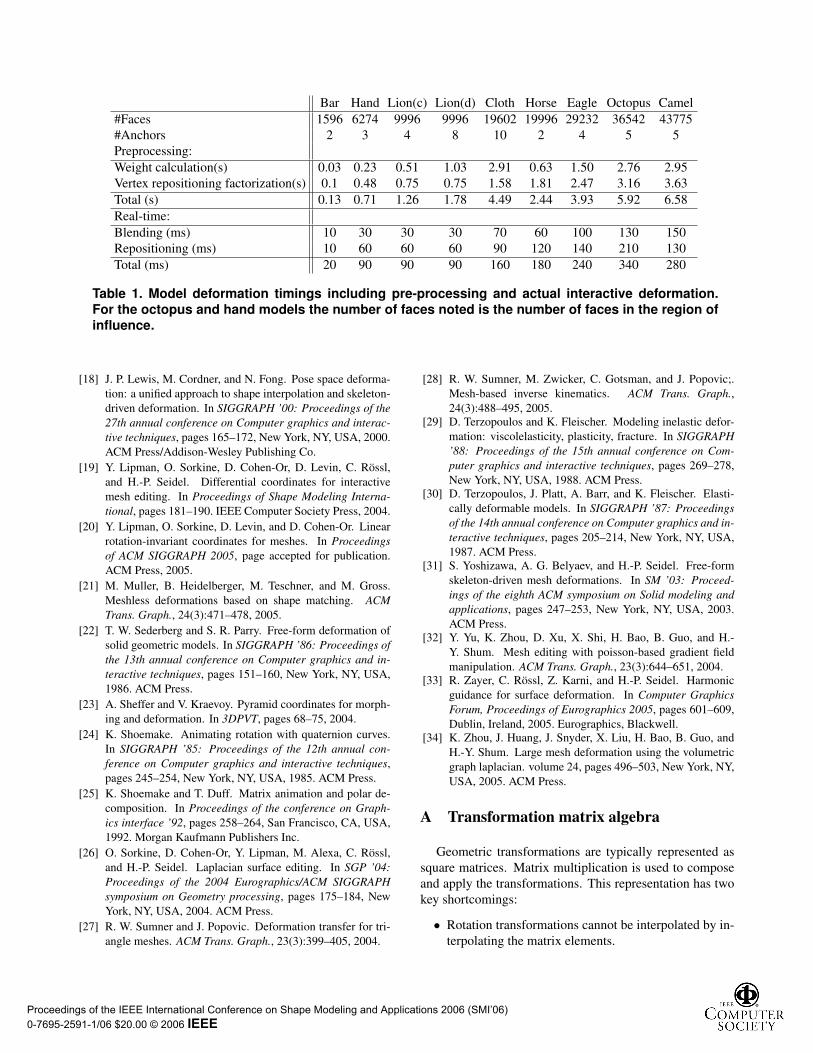
Bar Hand Lion(c) Lion(d) Cloth Horse Eagle Octopus Camel

#Faces 1596 6274 9996 9996 19602 19996 29232 36542 43775

#Anchors 2 3 4 8 10 2 4 5 5

Preprocessing:

Weight calculation(s) 0.03 0.23 0.51 1.03 2.91 0.63 1.50 2.76 2.95

Vertex repositioning factorization(s) 0.1 0.48 0.75 0.75 1.58 1.81 2.47 3.16 3.63

Total (s) 0.13 0.71 1.26 1.78 4.49 2.44 3.93 5.92 6.58

Real-time:

Blending (ms) 10 30 30 30 70 60 100 130 150

Repositioning (ms) 10 60 60 60 90 120 140 210 130

Total (ms) 20 90 90 90 160 180 240 340 280

Table 1. Model deformation timings including pre-processing and actual interactive deformation.For the octopus and hand models the number of faces noted is the number of faces in the region ofinfluence.

[18] J. P. Lewis, M. Cordner, and N. Fong. Pose space deforma-

tion: a unified approach to shape interpolation and skeleton-

driven deformation. In SIGGRAPH ’00: Proceedings of the27th annual conference on Computer graphics and interac-tive techniques, pages 165–172, New York, NY, USA, 2000.

ACM Press/Addison-Wesley Publishing Co.

[19] Y. Lipman, O. Sorkine, D. Cohen-Or, D. Levin, C. Rossl,

and H.-P. Seidel. Differential coordinates for interactive

mesh editing. In Proceedings of Shape Modeling Interna-tional, pages 181–190. IEEE Computer Society Press, 2004.

[20] Y. Lipman, O. Sorkine, D. Levin, and D. Cohen-Or. Linear

rotation-invariant coordinates for meshes. In Proceedingsof ACM SIGGRAPH 2005, page accepted for publication.

ACM Press, 2005.

[21] M. Muller, B. Heidelberger, M. Teschner, and M. Gross.

Meshless deformations based on shape matching. ACMTrans. Graph., 24(3):471–478, 2005.

[22] T. W. Sederberg and S. R. Parry. Free-form deformation of

solid geometric models. In SIGGRAPH ’86: Proceedings ofthe 13th annual conference on Computer graphics and in-teractive techniques, pages 151–160, New York, NY, USA,

1986. ACM Press.

[23] A. Sheffer and V. Kraevoy. Pyramid coordinates for morph-

ing and deformation. In 3DPVT, pages 68–75, 2004.

[24] K. Shoemake. Animating rotation with quaternion curves.

In SIGGRAPH ’85: Proceedings of the 12th annual con-ference on Computer graphics and interactive techniques,

pages 245–254, New York, NY, USA, 1985. ACM Press.

[25] K. Shoemake and T. Duff. Matrix animation and polar de-

composition. In Proceedings of the conference on Graph-ics interface ’92, pages 258–264, San Francisco, CA, USA,

1992. Morgan Kaufmann Publishers Inc.

[26] O. Sorkine, D. Cohen-Or, Y. Lipman, M. Alexa, C. Rossl,

and H.-P. Seidel. Laplacian surface editing. In SGP ’04:Proceedings of the 2004 Eurographics/ACM SIGGRAPHsymposium on Geometry processing, pages 175–184, New

York, NY, USA, 2004. ACM Press.

[27] R. W. Sumner and J. Popovic. Deformation transfer for tri-

angle meshes. ACM Trans. Graph., 23(3):399–405, 2004.

[28] R. W. Sumner, M. Zwicker, C. Gotsman, and J. Popovic;.

Mesh-based inverse kinematics. ACM Trans. Graph.,24(3):488–495, 2005.

[29] D. Terzopoulos and K. Fleischer. Modeling inelastic defor-

mation: viscolelasticity, plasticity, fracture. In SIGGRAPH’88: Proceedings of the 15th annual conference on Com-puter graphics and interactive techniques, pages 269–278,

New York, NY, USA, 1988. ACM Press.[30] D. Terzopoulos, J. Platt, A. Barr, and K. Fleischer. Elasti-

cally deformable models. In SIGGRAPH ’87: Proceedingsof the 14th annual conference on Computer graphics and in-teractive techniques, pages 205–214, New York, NY, USA,

1987. ACM Press.[31] S. Yoshizawa, A. G. Belyaev, and H.-P. Seidel. Free-form

skeleton-driven mesh deformations. In SM ’03: Proceed-ings of the eighth ACM symposium on Solid modeling andapplications, pages 247–253, New York, NY, USA, 2003.

ACM Press.[32] Y. Yu, K. Zhou, D. Xu, X. Shi, H. Bao, B. Guo, and H.-

Y. Shum. Mesh editing with poisson-based gradient field

manipulation. ACM Trans. Graph., 23(3):644–651, 2004.[33] R. Zayer, C. Rossl, Z. Karni, and H.-P. Seidel. Harmonic

guidance for surface deformation. In Computer GraphicsForum, Proceedings of Eurographics 2005, pages 601–609,

Dublin, Ireland, 2005. Eurographics, Blackwell.[34] K. Zhou, J. Huang, J. Snyder, X. Liu, H. Bao, B. Guo, and

H.-Y. Shum. Large mesh deformation using the volumetric

graph laplacian. volume 24, pages 496–503, New York, NY,

USA, 2005. ACM Press.

A Transformation matrix algebra

Geometric transformations are typically represented as

square matrices. Matrix multiplication is used to compose

and apply the transformations. This representation has two

key shortcomings:

• Rotation transformations cannot be interpolated by in-

terpolating the matrix elements.


• Matrix multiplication is not commutative.

Both of these properties are crucial for us in order to propa-

gate and later decompose anchor triangles.

To deal with these issues a number of interpolation

methods for rotations have been developed over the years.

When dealing with rotations there are three desired prop-

erties: torque-minimization, constant speed, and commuta-

tivity. Currently no interpolation method exhibiting all three

properties exists. SLERP [24] exhibits constant speed and

minimal-torque. LERP, popularized by Casey Muratori, is

commutative and minimal-torque. The exponential map in-

terpolation [13] is commutative and constant speed.

Alexa [2] extended the exponential map interpolation

method into a commutative algebra of (almost) general

transformations that supports matrix blending and interpo-

lation. This algebra is commutative and interpolates trans-

formations with constant speed. Furthermore, it is not lim-

ited to rotations only, thus simplifying the task of dealing

with combinations of rotations and scales.

We have chosen to use the later method since it answers

both our requirements. We now give a brief overview of the

blending operators defined in this algebra.

By defining two new operations denoted by ⊕ and by

� (corresponding to matrix addition and scalar multiplica-

tion), the blending of transformations Ta with weights ωabecomes

⊕ωa �Ta.

The two operators are based on matrix exp and log oper-

ators defined as follows:

exp(A) =∞

∑k=0

Ak

k!,

A = log(X) ⇔ exp(A) = X .

Alexa [2] shows that this sum is well defined and closed

for 3x3 rotation matrices and non-uniform scales under

some minimal conditions. The blending formula is defined

as follows:

k⊕a=1

ωai �Ta = exp(

k

∑a=1

ωai log(Ta)).

More details as well as numerical methods to compute

these operations are found in [2].


Documents

Material-Aware Mesh Deformationsmesh.brown.edu/DGP/pdfs/Popa-smi2006.pdf · Material-Aware Mesh Deformations ... Most real world objects consist of non-uniform materi-als; as a result,