Material and geometric nonlinear analysis of reinforced ... · 880 IBRACON Structures and Materials Journal • 2014 • vol. 7 • n 5 Material and geometric nonlinear analysis of

Volume 7, Number 5 (October 2014) p. 879-904 • ISSN 1983-4195

© 2014 IBRACON

Material and geometric nonlinear analysis of reinforced concrete frames

Análise não linear física e geométrica de pórticos de concreto armado

a Universidade Federal do Ceará, Fortaleza, CE, Brasil.

Received: 02 Sep 2013 • Accepted: 24 Jul 2014 • Available Online: 02 Oct 2014

Abstract

Resumo

The analysis of reinforced concrete structures until failure requires the consideration of geometric and material nonlinearities. However, nonlinear analysis is much more complex and costly than linear analysis. In order to obtain a computationally efficient approach to nonlinear analysis of reinforced concrete structures, this work presents the formulation of a nonlinear plane frame element. Geometric nonlinearity is considered using the co-rotational approach and material nonlinearity is included using appropriate constitutive relations for concrete and steel. The integration of stress resultants and tangent constitutive matrix is carried out by the automatic subdivision of the cross-section and the application of the Gauss quadrature in each subdivision. The formulation and computational implementation are validated using experimental results available in the litera-ture. Excellent results were obtained.

Keywords: concrete structures, nonlinear analysis, plane frames, finite element method.

A análise de estruturas de concreto armado até à ruína requer a consideração das não linearidades física e geométrica. Contudo, a análise não linear é mais complexa e possui custo computacional mais elevado que a análise linear. Com objetivo de obter uma alternativa eficiente para a análise não linear de estruturas reticuladas de concreto armado, este trabalho apresenta a formulação de um elemento finito de pórtico plano não linear. A não linearidade geométrica é tratada através do uso da formulação corrotacional e a não linearidade física é considerada através do uso de relações constitutivas apropriadas para o concreto e o aço. A integração dos esforços e da matriz constitutiva tangente é realizada pela subdivisão automática da seção transversal em faixas seguida pela uso da quadratura de Gauss em cada faixa. A formulação e implementação computacional são validadas através da comparação com resultados experimentais, tendo sido obtidos excelentes resultados..

Palavras-chave: estruturas de concreto, análise não linear, pórticos planos, método dos elementos finitos.

E. PAREntE JR a

[email protected]

G. V. noGuEiRA a

[email protected]

M. MEiRElEs nEto a

[email protected]

l. s. MoREiRA a

[email protected]

880 IBRACON Structures and Materials Journal • 2014 • vol. 7 • nº 5


1. introduction

The structures of reinforced concrete buildings are constituted main-ly of beams and columns rigidly connected, forming plane frames. The simulation of the behavior of these structures in a realistic way, especially near failure, requires the consideration of material nonlin-earity, due to the presence of effects such as concrete cracking and reinforcement yielding, as well geometric nonlinearity, due to large displacements and high compressive forces. The search for more economical designs, the use of high strength materials and slender structures has increased the importance of nonlinear analysis.Concrete has a highly complex mechanical behavior. Thus, plane and solid elements with two and three dimensional constitutive models have been used in the computational modeling of lab tests. These constitutive models allow representing the effects of stress state on concrete behavior, leading to an excellent agreement of the numerical and experimental load-displacement curves [11].However, this approach is not feasible for the analysis of building structures formed by a large number of members (columns and beams) due to the high computational cost, besides the difficulty of geometric modeling and mesh generation. On the other hand, the design of building structures is generally carried out using linear analysis and frame elements. The effect of nonlinearity is consid-ered approximately using the secant modulus to represent the ma-terial nonlinearity and the parameter zγ to estimate the second-order effects (geometric nonlinearity) [1].In order to perform the nonlinear analysis of reinforced concrete reticulated structures simple and efficient way, this paper presents the formulation of a plane frame finite element for geometrical and material nonlinear analysis. The geometric nonlinearity is consid-

ered by using the co-rotational formulation, allowing the analysis of structures with large displacements and rotations.The material nonlinearity is considered using nonlinear stress-strain relationships for steel and concrete in compression present-ed in standards NBR 6118:2007 [1] and Eurocode 2:2004 [7]. The contribution of the concrete in tension (tension stiffening) is consid-ered using the CEB model [10]. A new method for the integration of stresses and the constitutive matrix over reinforced concrete cross-sections is proposed in this paper. This method is based on the automatic subdivision of the cross-section in accordance with the ranges of the stress-strain curves and the use of Gaussian quadrature for each segment, resulting in a simple, efficient and accurate formulation. Moreover, this method is independent of the stress-strain curve adopted.The formulations and implementations are evaluated through com-parison with experimental and numerical results available in the literature. This work presents an assessment of the influence of the finite element discretization and the number of points used for cross-section integration.

2. Planeframeco-rotationalfiniteelement

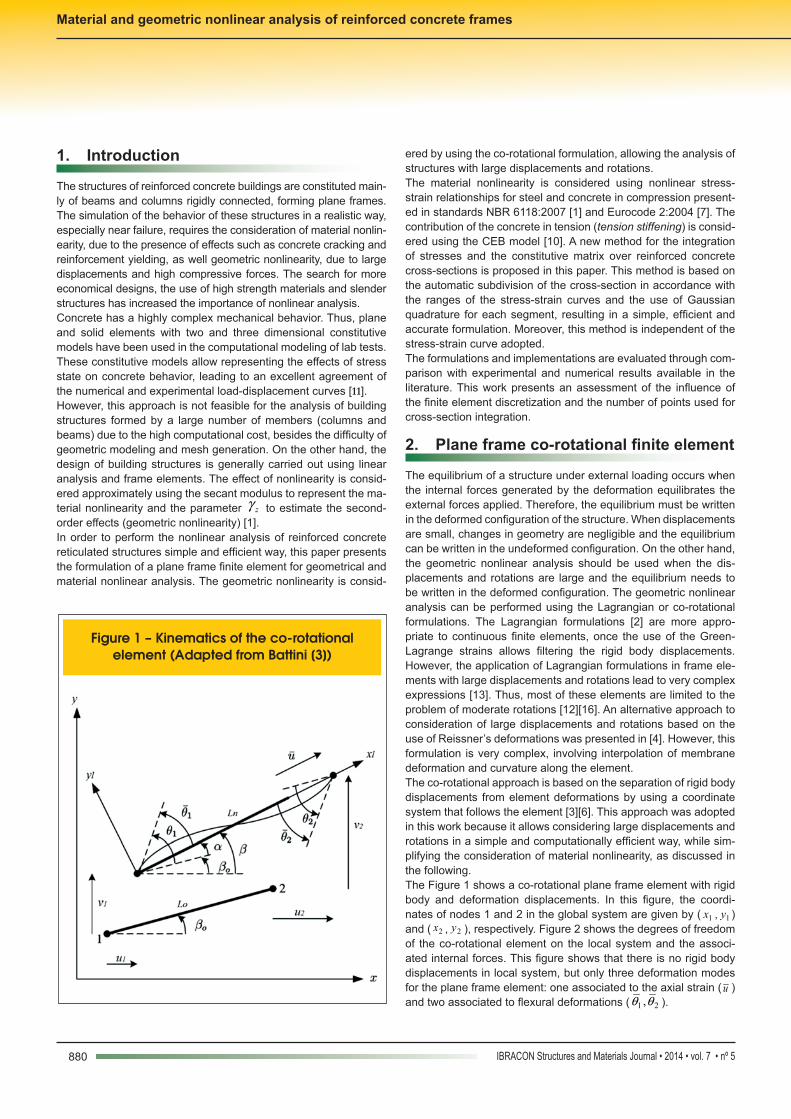
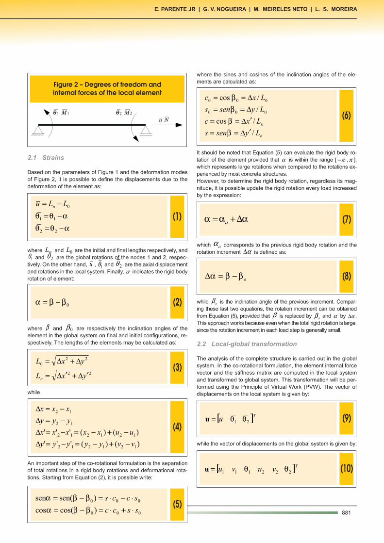
The equilibrium of a structure under external loading occurs when the internal forces generated by the deformation equilibrates the external forces applied. Therefore, the equilibrium must be written in the deformed configuration of the structure. When displacements are small, changes in geometry are negligible and the equilibrium can be written in the undeformed configuration. On the other hand, the geometric nonlinear analysis should be used when the dis-placements and rotations are large and the equilibrium needs to be written in the deformed configuration. The geometric nonlinear analysis can be performed using the Lagrangian or co-rotational formulations. The Lagrangian formulations [2] are more appro-priate to continuous finite elements, once the use of the Green-Lagrange strains allows filtering the rigid body displacements. However, the application of Lagrangian formulations in frame ele-ments with large displacements and rotations lead to very complex expressions [13]. Thus, most of these elements are limited to the problem of moderate rotations [12][16]. An alternative approach to consideration of large displacements and rotations based on the use of Reissner’s deformations was presented in [4]. However, this formulation is very complex, involving interpolation of membrane deformation and curvature along the element.The co-rotational approach is based on the separation of rigid body displacements from element deformations by using a coordinate system that follows the element [3][6]. This approach was adopted in this work because it allows considering large displacements and rotations in a simple and computationally efficient way, while sim-plifying the consideration of material nonlinearity, as discussed in the following.The Figure 1 shows a co-rotational plane frame element with rigid body and deformation displacements. In this figure, the coordi-nates of nodes 1 and 2 in the global system are given by ( 1x , 1y ) and ( 2x , 2y ), respectively. Figure 2 shows the degrees of freedom of the co-rotational element on the local system and the associ-ated internal forces. This figure shows that there is no rigid body displacements in local system, but only three deformation modes for the plane frame element: one associated to the axial strain ( u ) and two associated to flexural deformations ( 21 ,θθ ).

Figure 1 – Kinematics of the co-rotational element (Adapted from Battini [3])

881IBRACON Structures and Materials Journal • 2014 • vol. 7 • nº 5

E. ParEntE Jr | G. V. noGuEira | M. MEirElEs nEto | l. s. MorEira

2.1 Strains

Based on the parameters of Figure 1 and the deformation modes of Figure 2, it is possible to define the displacements due to the deformation of the element as:

(1)

aqqaqq-=-=-=

22

11

0LLu n

where nL and 0L are the initial and final lengths respectively, and 1θ and 2θ are the global rotations of the nodes 1 and 2, respec-

tively. On the other hand, u , 1θ and 2θ are the axial displacement and rotations in the local system. Finally, α indicates the rigid body rotation of element:

(2) 0bba -=

where β and 0β are respectively the inclination angles of the element in the global system on final and initial configurations, re-spectively. The lengths of the elements may be calculated as:

(3)

22

220

yxL

yxL

n¢D+¢D=

D+D=

while

(4)

)()('''

)()('''

121212

121212

12

12

vvyyyyy

uuxxxxx

yyy

xxx

-+-=-=D-+-=-=D

-=D-=D

An important step of the co-rotational formulation is the separation of total rotations in a rigid body rotations and deformational rota-tions. Starting from Equation (2), it is possible write:

(5)

000

000

)cos(cos

)(sensen

sscc

sccs

×+×=-=×-×=-=

bbabba

where the sines and cosines of the inclination angles of the ele-ments are calculated as:

(6)

n

n

Lysens

Lxc

Lysens

Lxc

/

/cos

/

/cos

000

000

¢D==¢D==D==D==

bbbb

It should be noted that Equation (5) can evaluate the rigid body ro-tation of the element provided that α is within the range [ π− ,π ], which represents large rotations when compared to the rotations ex-perienced by most concrete structures.However, to determine the rigid body rotation, regardless its mag-nitude, it is possible update the rigid rotation every load increased by the expression:

(7) aaa D+= a

which aα corresponds to the previous rigid body rotation and the rotation increment α∆ is defined as:

(8) abba -=D

while aβ is the inclination angle of the previous increment. Compar-ing these last two equations, the rotation increment can be obtained from Equation (5), provided that β is replaced by aβ and α by α∆ . This approach works because even when the total rigid rotation is large, since the rotation increment in each load step is generally small.

2.2 Local-global transformation

The analysis of the complete structure is carried out in the global system. In the co-rotational formulation, the element internal force vector and the stiffness matrix are computed in the local system and transformed to global system. This transformation will be per-formed using the Principle of Virtual Work (PVW). The vector of displacements on the local system is given by:

(9) [ ]Tu 21 qq=u

while the vector of displacements on the global system is given by:

(10) [ ]Tvuvu 222111 qq=u

Figure 2 – Degrees of freedom and internal forces of the local element



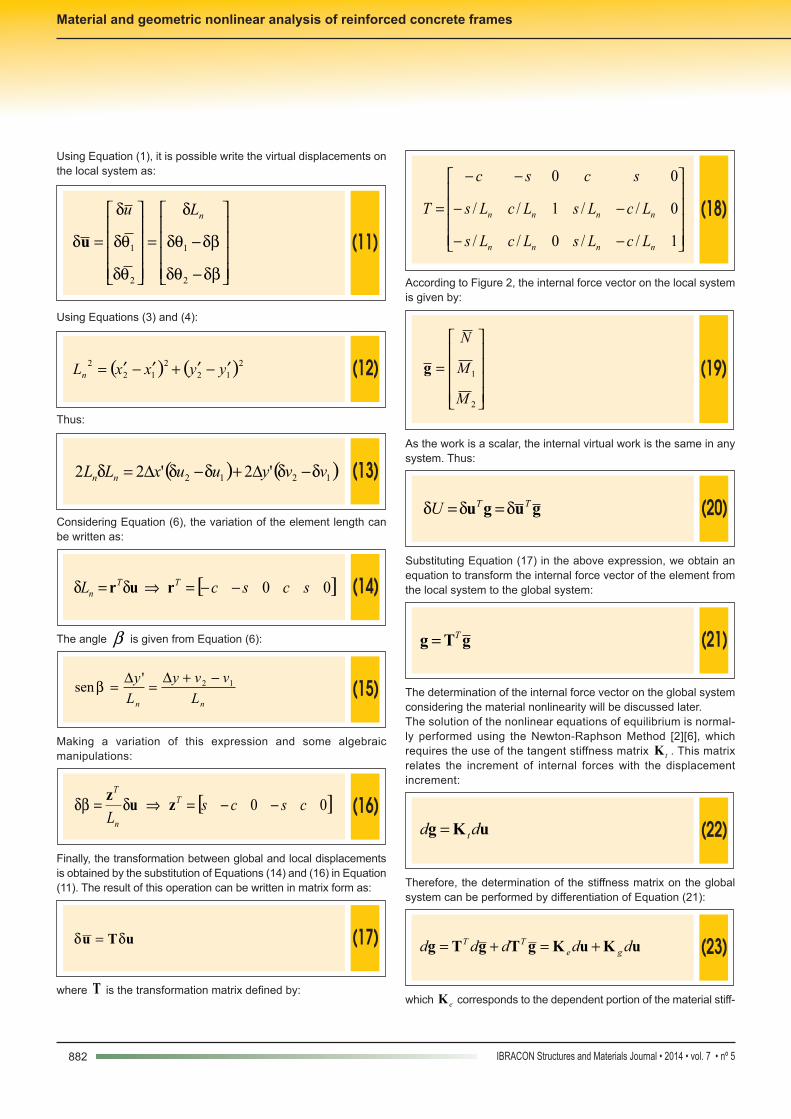
Using Equation (1), it is possible write the virtual displacements on the local system as:

(11)

úúúú

û

ù

êêêê

ë

é

-

-=

úúúú

û

ù

êêêê

ë

é

=

dbdq

dbdq

d

qd

qd

d

d

2

1

2

1

nLu

u

Using Equations (3) and (4):

(12) ( ) ( )212

2

12

2yyxxLn¢-¢+¢-¢=

Thus:

(13) ( ) ( )1212 '2'22 vvyuuxLL nn ddddd -D+-D=

Considering Equation (6), the variation of the element length can be written as:

(14) [ ]00 scscL TTn --=Þ= rur dd

The angle β is given from Equation (6):

(15)

nn L

vvy

L

y 12'sen

-+D=D=b

Making a variation of this expression and some algebraic manipulations:

(16)

[ ]00 cscsL

T

n

T

--=Þ= zuz ddb

Finally, the transformation between global and local displacements is obtained by the substitution of Equations (14) and (16) in Equation (11). The result of this operation can be written in matrix form as:

(17) uTu dd =

where T is the transformation matrix defined by:

(18)

úúúú

û

ù

êêêê

ë

é

--

--

--

=

1//0//

0//1//

00

nnnn

nnnn

LcLsLcLs

LcLsLcLs

scsc

T

According to Figure 2, the internal force vector on the local system is given by:

(19)

úúúú

û

ù

êêêê

ë

é

=

2

1

M

M

N

g

As the work is a scalar, the internal virtual work is the same in any system. Thus:

(20) gugu TTU ddd ==

Substituting Equation (17) in the above expression, we obtain an equation to transform the internal force vector of the element from the local system to the global system:

(21) gTg T=

The determination of the internal force vector on the global system considering the material nonlinearity will be discussed later. The solution of the nonlinear equations of equilibrium is normal-ly performed using the Newton-Raphson Method [2][6], which requires the use of the tangent stiffness matrix tK . This matrix relates the increment of internal forces with the displacement increment:

(22) uKg dd t=

Therefore, the determination of the stiffness matrix on the global system can be performed by differentiation of Equation (21):

(23) uKuKgTgTg ddddd geTT +=+=

which eK corresponds to the dependent portion of the material stiff-



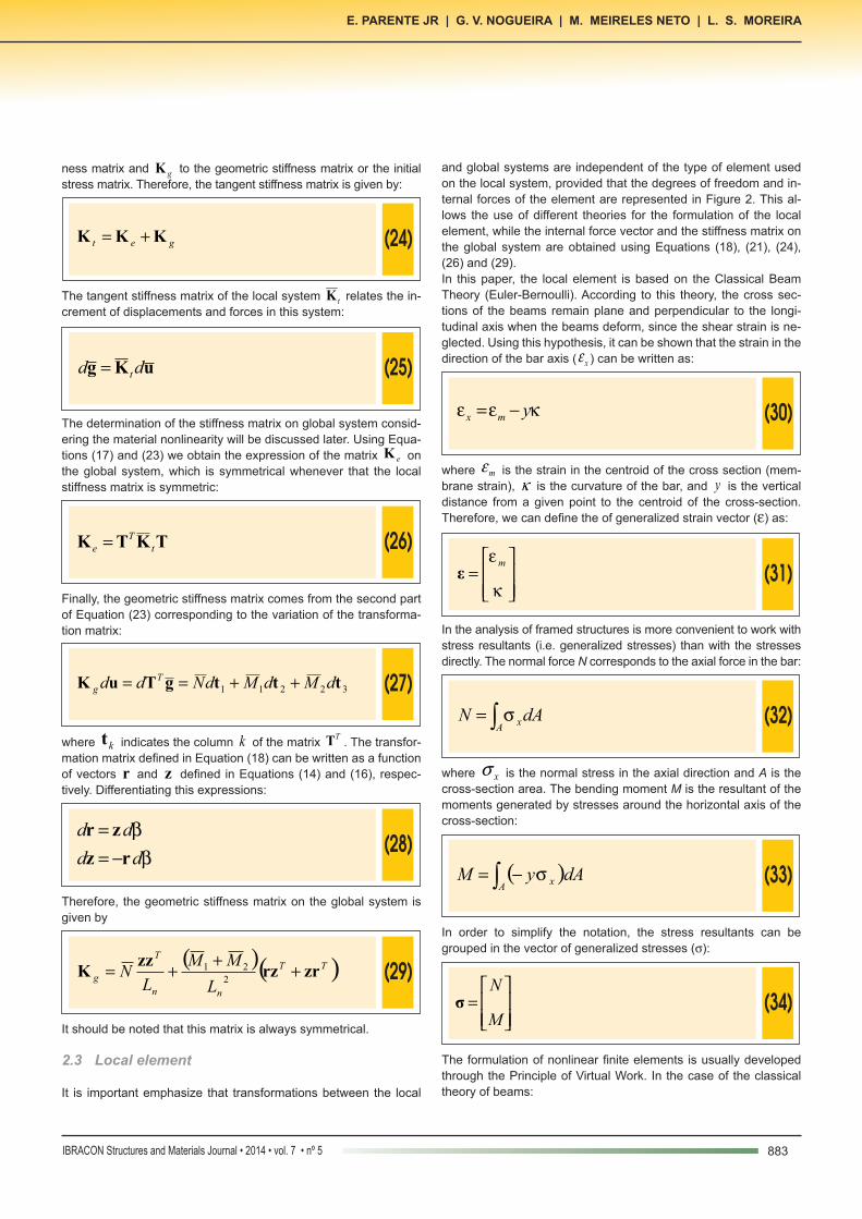
ness matrix and gK to the geometric stiffness matrix or the initial stress matrix. Therefore, the tangent stiffness matrix is given by:

(24) get KKK +=

The tangent stiffness matrix of the local system tK relates the in-crement of displacements and forces in this system:

(25) uKg dd t=

The determination of the stiffness matrix on global system consid-ering the material nonlinearity will be discussed later. Using Equa-tions (17) and (23) we obtain the expression of the matrix eK on the global system, which is symmetrical whenever that the local stiffness matrix is symmetric:

(26) TKTK tT

e =

Finally, the geometric stiffness matrix comes from the second part of Equation (23) corresponding to the variation of the transforma-tion matrix:

(27) 32211 tttgTuK dMdMdNdd T

g ++==

where kt indicates the column k of the matrix TT . The transfor-mation matrix defined in Equation (18) can be written as a function of vectors r and z defined in Equations (14) and (16), respec-tively. Differentiating this expressions:

(28)

bbdd

dd

rz

zr

-==

Therefore, the geometric stiffness matrix on the global system is given by

(29) ( )( )TT

nn

T

gL

MM

LN zrrz

zzK +++=

2

21

It should be noted that this matrix is always symmetrical.

2.3 Local element

It is important emphasize that transformations between the local

and global systems are independent of the type of element used on the local system, provided that the degrees of freedom and in-ternal forces of the element are represented in Figure 2. This al-lows the use of different theories for the formulation of the local element, while the internal force vector and the stiffness matrix on the global system are obtained using Equations (18), (21), (24), (26) and (29).In this paper, the local element is based on the Classical Beam Theory (Euler-Bernoulli). According to this theory, the cross sec-tions of the beams remain plane and perpendicular to the longi-tudinal axis when the beams deform, since the shear strain is ne-glected. Using this hypothesis, it can be shown that the strain in the direction of the bar axis ( xe ) can be written as:

(30) kee ymx -=

where me is the strain in the centroid of the cross section (mem-brane strain), κ is the curvature of the bar, and y is the vertical distance from a given point to the centroid of the cross-section. Therefore, we can define the of generalized strain vector (e) as:

(31)

úúû

ù

êêë

é=

k

em

ε

In the analysis of framed structures is more convenient to work with stress resultants (i.e. generalized stresses) than with the stresses directly. The normal force N corresponds to the axial force in the bar:

(32) ò= AxdAN s

where xs is the normal stress in the axial direction and A is the cross-section area. The bending moment M is the resultant of the moments generated by stresses around the horizontal axis of the cross-section:

(33) ( )ò -=A

x dAyM s

In order to simplify the notation, the stress resultants can be grouped in the vector of generalized stresses (s):

(34)

úúû

ù

êêë

é=

M

Nσ

The formulation of nonlinear finite elements is usually developed through the Principle of Virtual Work. In the case of the classical theory of beams:



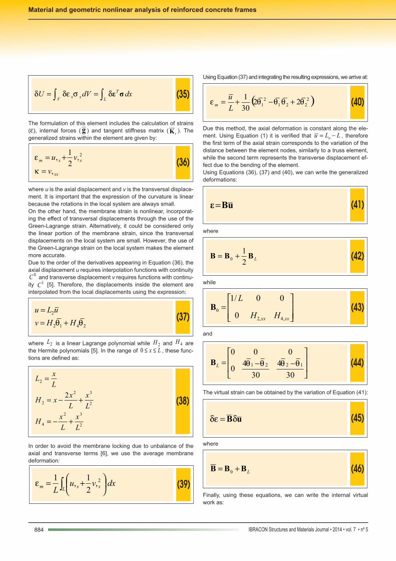
(35) dxdVUL

T

Vxx òò == σεdsded

The formulation of this element includes the calculation of strains (e), internal forces ( g ) and tangent stiffness matrix ( tK ). The generalized strains within the element are given by:

(36)

xx

xxm

v

vu

,

,2

1, 2

=

+=

k

e

where u is the axial displacement and v is the transversal displace-ment. It is important that the expression of the curvature is linear because the rotations in the local system are always small.On the other hand, the membrane strain is nonlinear, incorporat-ing the effect of transversal displacements through the use of the Green-Lagrange strain. Alternatively, it could be considered only the linear portion of the membrane strain, since the transversal displacements on the local system are small. However, the use of the Green-Lagrange strain on the local system makes the element more accurate.Due to the order of the derivatives appearing in Equation (36), the axial displacement u requires interpolation functions with continuity

0C and transverse displacement v requires functions with continu-ity 1C [5]. Therefore, the displacements inside the element are interpolated from the local displacements using the expression:

(37)

2412

2

qq HHv

uLu

+==

where 2L is a linear Lagrange polynomial while 2H and 4H are the Hermite polynomials [5]. In the range of Lx ≤≤0 , these func-tions are defined as:

(38)

2

32

4

2

32

2

2

2

L

x

L

xH

L

x

L

xxH

L

xL

+-=

+-=

=

In order to avoid the membrane locking due to unbalance of the axial and transverse terms [6], we use the average membrane deformation:

(39)

ò ÷øöç

èæ +=

L xxm dxvuL

2,2

1,

1e

Using Equation (37) and integrating the resulting expressions, we arrive at:

(40) ( )22212

1 2230

1 qqqqe +-+=L

um

Due this method, the axial deformation is constant along the ele-ment. Using Equation (1) it is verified that LLu n −= , therefore the first term of the axial strain corresponds to the variation of the distance between the element nodes, similarly to a truss element, while the second term represents the transverse displacement ef-fect due to the bending of the element.Using Equations (36), (37) and (40), we can write the generalized deformations:

(41) uBε=

where

(42)

LBBB2

10 +=

while

(43)

úúû

ù

êêë

é=

xxxx HH

L

,4,2

00

00/1B

and

(44)

úú

û

ù

êê

ë

é--=

30

4

30

40

000

1221 qqqqLB

The virtual strain can be obtained by the variation of Equation (41):

(45) uBdde =

where

(46) LBBB += 0

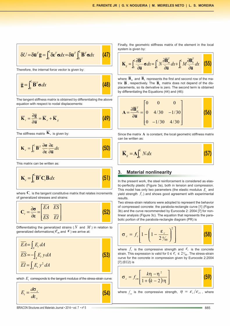
Finally, using these equations, we can write the internal virtual work as:



(47)

ò ò===L L

TTTT dxdxU0 0

σBuσεgu dddd

Therefore, the internal force vector is given by:

(48)

ò=L

T dx0

σBg

The tangent stiffness matrix is obtained by differentiating the above equation with respect to nodal displacements:

(49) get KK

u

gK +=

¶¶=

The stiffness matrix eK is given by:

(50) ò ¶

¶¶¶=

LT

e dx0 u

ε

ε

σBK

This matrix can be written as:

(51)

ò=L

tT

e dx0

BCBK

where tC is the tangent constitutive matrix that relates increments of generalized stresses and strains:

(52)

úúû

ù

êêë

é=

¶¶=

EIES

ESEAt

ε

σC

Differentiating the generalized strains ( N and M ) in relation to generalized deformations( me and κ ) we arrive at:

(53)

òòò

=

-=

=

At

At

At

dAyEEI

dAyEES

dAEEA

2

which tE corresponds to the tangent modulus of the stress-strain curve:

(54)

x

xt

d

dE

es=

Finally, the geometric stiffness matrix of the element in the local system is given by:

(55)

òòò ¶¶

+¶¶

=¶¶=

LTb

LTm

LT

g dxMdxNdx000 u

B

u

Bσ

u

BK

where mB and bB represents the first and second row of the ma-trix B , respectively. The bB matrix does not depend of the dis-placements, so its derivative is zero. The second term is obtained by differentiating the Equations (44) and (46):

(56)

úúúú

û

ù

êêêê

ë

é

-

-=¶¶=

30/430/10

30/130/40

000

u

BA

Tm

Since the matrix A is constant, the local geometric stiffness matrix can be written as:

(57)

ò=L

g dxN0

AK

3. Material nonlinearity

In the present work, the steel reinforcement is considered as elas-tic-perfectly plastic (Figure 3a), both in tension and compression. This model has only two parameters (the elastic modulus sE and yield strength yf ) and shows good agreement with experimental results. Two stress-strain relations were adopted to represent the behavior of compressed concrete: the parabola-rectangle curve [1] (Figure 3b) and the curve recommended by Eurocode 2: 2004 [7] for non-linear analysis (Figure 3c). The equation that represents the para-bolic portion of the parabola-rectangle diagram (PR) is

(58)

úúû

ù

êêë

é÷÷ø

öççè

æ --=2

0002

11 ccc f

es

where cf is the compressive strength and ce is the concrete strain. This expression is valid for 0 ≤ ce ≤ 2 0

00 . The stress-strain curve for the concrete in compression given by Eurocode 2:2004 [7] (EC2) is

(59)

( ) úúû

ù

êêë

é-+-=

hhhs21

2

k

kfcmc

where fcm is the compressive strength, 1cc eeη = , where



ec1 is the strain at peak stress, cmccm fEk 105.1 e= and

cmE is the secant modulus corresponding to

cmf4.0 stress, as indicated in Figure 3c. Equation (59) is valid for

10 cuc ee << , where

000

1 5.3=cue . It is important to note that this curve considers the softening of concrete after the peak stress, while the parabola-curved rectangle considers a constant stress between 2 0

00 and 00

05.3 . For both curves it is considered the concrete is completely crushed ( 0=cs ) for strains greater than 00

05.3 . The behavior of plain concrete under uniaxial tensile stresses can be represented by a bilinear curve [1], where after the first crack the concrete loses all resistance. However, in reinforced concrete, tensile stresses between cracks can be transmitted from the steel to the concrete around the steel bar by means of bond stresses between reinforcement and adjacent concrete. This effect is known as tension stiffening [17].In this work, the tension stiffening is considered using the formula-

tion presented in [10]. This formulation is based on the CEB model, developed from tests of reinforced concrete specimens subjected to uniaxial tension. In the adopted model, the tensile stresses (sct) in the cracked concrete are calculated by the expression:

(60)

( )hrerers ++÷øöç

èæ+-= 122

22

ctcscsct fEE

where fct is the tensile strength of concrete, cs EE /=η and ρ is the effective reinforcement ratio (

efcs AA ,/=r ), where Ac,ef is the effective concrete area (i.e. the area contributing to tension stiff-ening). The CEB-FIP 1990 recommends using ( )dhbA efc -= 5.2, , where b is the cross-section width, h is the height, and d is the effective depth of reinforcement. The stress-strain relation of ten-

Figure 3 – Stress-strain curves

A

C

B

D

Steel

Eurocode 2 [7]

Parabola-rectangle

Concrete – tension



sioned concrete (TS) is composed of a linear curve until cracking (sct = fct) followed by a softening portion, given by Equation (60), until the yield of rebars (ey). This curve is illustrated in Figure 3d. It is important to note that the formulations presented in this paper allow the adoption of different stress-strain curves to model the be-havior of steel and concrete. Thus, the stress-strain relationships described in this section and represented in Figure 3 were chosen for computer implementation due to its wide use in literature and good agreement with experimental results.

3.1 Cross-section integration

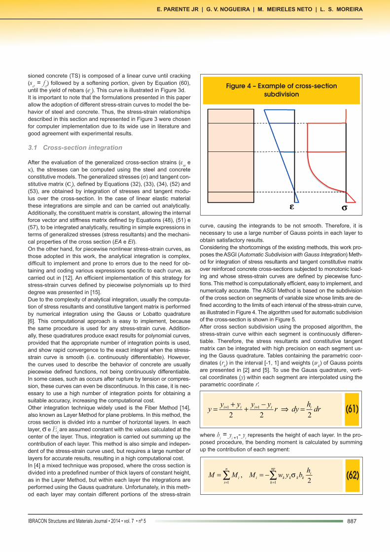
After the evaluation of the generalized cross-section strains (em e κ), the stresses can be computed using the steel and concrete constitutive models. The generalized stresses (s) and tangent con-stitutive matrix (Ct), defined by Equations (32), (33), (34), (52) and (53), are obtained by integration of stresses and tangent modu-lus over the cross-section. In the case of linear elastic material these integrations are simple and can be carried out analytically. Additionally, the constituent matrix is constant, allowing the internal force vector and stiffness matrix defined by Equations (48), (51) e (57), to be integrated analytically, resulting in simple expressions in terms of generalized stresses (stress resultants) and the mechani-cal properties of the cross section (EA e EI).On the other hand, for piecewise nonlinear stress-strain curves, as those adopted in this work, the analytical integration is complex, difficult to implement and prone to errors due to the need for ob-taining and coding various expressions specific to each curve, as carried out in [12]. An efficient implementation of this strategy for stress-strain curves defined by piecewise polynomials up to third degree was presented in [15].Due to the complexity of analytical integration, usually the computa-tion of stress resultants and constitutive tangent matrix is performed by numerical integration using the Gauss or Lobatto quadrature [6]. This computational approach is easy to implement, because the same procedure is used for any stress-strain curve. Addition-ally, these quadratures produce exact results for polynomial curves, provided that the appropriate number of integration points is used, and show rapid convergence to the exact integral when the stress-strain curve is smooth (i.e. continuously differentiable). However, the curves used to describe the behavior of concrete are usually piecewise defined functions, not being continuously differentiable. In some cases, such as occurs after rupture by tension or compres-sion, these curves can even be discontinuous. In this case, it is nec-essary to use a high number of integration points for obtaining a suitable accuracy, increasing the computational cost. Other integration technique widely used is the Fiber Method [14], also known as Layer Method for plane problems. In this method, the cross section is divided into a number of horizontal layers. In each layer, s e Et are assumed constant with the values calculated at the center of the layer. Thus, integration is carried out summing up the contribution of each layer. This method is also simple and indepen-dent of the stress-strain curve used, but requires a large number of layers for accurate results, resulting in a high computational cost. In [4] a mixed technique was proposed, where the cross section is divided into a predefined number of thick layers of constant height, as in the Layer Method, but within each layer the integrations are performed using the Gauss quadrature. Unfortunately, in this meth-od each layer may contain different portions of the stress-strain

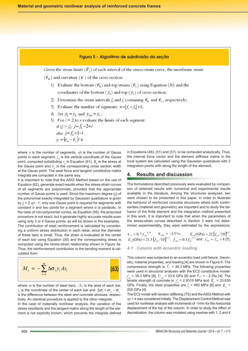
curve, causing the integrands to be not smooth. Therefore, it is necessary to use a large number of Gauss points in each layer to obtain satisfactory results.Considering the shortcomings of the existing methods, this work pro-poses the ASGI (Automatic Subdivision with Gauss Integration) Meth-od for integration of stress resultants and tangent constitutive matrix over reinforced concrete cross-sections subjected to monotonic load-ing and whose stress-strain curves are defined by piecewise func-tions. This method is computationally efficient, easy to implement, and numerically accurate. The ASGI Method is based on the subdivision of the cross section on segments of variable size whose limits are de-fined according to the limits of each interval of the stress-strain curve, as illustrated in Figure 4. The algorithm used for automatic subdivision of the cross-section is shown in Figure 5. After cross section subdivision using the proposed algorithm, the stress-strain curve within each segment is continuously differen-tiable. Therefore, the stress resultants and constitutive tangent matrix can be integrated with high precision on each segment us-ing the Gauss quadrature. Tables containing the parametric coor-dinates (rk) in the interval [-1, 1] and weights (wk) of Gauss points are presented in [2] and [5]. To use the Gauss quadrature, verti-cal coordinates (y) within each segment are interpolated using the parametric coordinate r:

(61)

drh

dyryyyy

y iiiii

22211 =Þ-++= ++

where hi = yi +1- yi represents the height of each layer. In the pro-posed procedure, the bending moment is calculated by summing up the contribution of each segment:

(62)

2,

11

inp

kkkkki

n

ii

hbywMMM åå

==

-== s

Figure 4 – Example of cross-section subdivision



where n is the number of segments, np is the number of Gauss points in each segment, yk is the vertical coordinate of the Gauss point, computed substituting rk in Equation (61), sk is the stress at the Gauss point and bk is the corresponding cross section width at the Gauss point. The axial force and tangent constitutive matrix integrals are computed in the same way. It is important to note that the ASGI Method based on the use of Equation (62), generate exact results when the stress-strain curves of all segments are polynomials, provided that the appropriate number of Gauss points is used. Since the maximum degree (g) of the polynomial exactly integrated by Gaussian quadrature is given by g = 2 np - 1, only one Gauss point is required for segments with constant s and two points for a segment where σ is parabolic. In the case of non-polynomial curves, as Equation (59), the proposed procedure is not exact, but it generate highly accurate results even using only 3 or 4 Gauss points, as will be shown in the examples.The contribution of steel reinforcement is calculated by consider-ing a uniform stress distribution in each rebar, since the diameter of these bars is small. Thus, the strain is evaluated at the center of each bar using Equation (30) and the corresponding stress is computed using the stress-strain relationship shown in Figure 3a. Thus, the reinforcement contribution to the bending moment is cal-culated from:

(63)

å=D-=

m

iiiis AsyM

1

s

where m is the number of steel bars, Asi is the area of each bar, yi is the coordinate of the center of each bar and

ii csi sss −=∆ is the difference between the steel and concrete stresses, respec-tively. An identical procedure is applied to the other integrals.In the case of materially nonlinear analysis, the variation of the stress resultants and the tangent matrix along the length of the ele-ment is not explicitly known, which prevents the integrals defined

in Equations (48), (51) and (57), to be computed analytically. Thus, the internal force vector and the element stiffness matrix in the local system are calculated using the Gaussian quadrature with 2 integration points with along the length of the element.

4. Results and discussion

The formulations described previously were evaluated by compari-son of obtained results with numerical and experimental results available in the literature. Among the structures analyzed, two were chosen to be presented in this paper, in order to illustrate the behavior of reinforced concrete structures where both nonlin-earities (material and geometric) are important and to study the be-havior of the finite element and the integration method presented in this work. It is important to note that when the parameters of the stress-strain curves described in Section 3 were not deter-mined experimentally, they were estimated by the expressions:

31.0

1 7.0 cmc f=e , 1cue = -3.5‰ , [ ] 3.010/ 22(GPa) cmcm fE = ,

[ ] 3/110/ 5.21(GPa) cmci fE = , 3/2

3.0 ckctm ff = and 8+= ckcm ff [7].

4.1 Column with eccentric loading

This column was subjected to an eccentric load until failure. Geom-etry, material properties, and loading [4] are shown in Figure 6. The compressive strength is cf = 38.3 MPa. The following properties were used in structural analyses with the EC2 constitutive model: fcm = 38.3 MPa [8], Ecm = 33.6 GPa [8] and 1ce = - 2.3‰ [4]. The tensile strength of concrete is fct = 2.9315 MPa and cE = 33.639 GPa. Finally, the steel properties are fy = 465 MPa [8] and sE = 200 GPa [4]. The EC2 model with tension stiffening (TS) and the ASGI Method with np = 4 was considered initially. The Displacement Control Method was used for nonlinear analysis with increments of -1mm for the horizontal displacement of the top of the column. In order to study the effect of discretization, the column was modeled using meshes with 1, 2 and 4

Figura 5 – Algoritmo de subdivisão da seção



elements, obtaining the maximum loads of 457.52 kN, 460.59 kN and 460.09 kN, respectively. These results are in excellent agreement with the maximum load of 454 kN obtained experimentally [8], showing that the proposed formulation does not require very fine meshes to adequately represent the material and geometric nonlinear behavior of the structure. It is important to note that the maximum load obtained in this work was closer to the experimental load than the maximum load (445 kN) obtained in [4] using the EC2 model without the tension stiffening effect. It was also found that the Newton-Raphson Method presented quadratic convergence, with the number of iterations rang-ing between 3 and 4 throughout the analysis, even using a very tight tolerance used for convergence (10-8).Next, the influence of the integration method, number of layers (nf) and Gauss points (np) was assessed using a fixed number of elements (4) and constitutive model (EC2 with TS). The results obtained are shown in Table 1. These results show that the use of 20 layers generate satisfactory results. However, the ASGI Method is more accurate and efficient than the Layer Method, generating better results using just 2 Gauss points per segment than the Layer Method with 20 layers. Additionally, accurate results with six sig-nificant figures, which require the use of 600 layers, are obtained using only 3 Gauss points per segment. Note that [4] used 5 lay-

ers of fixed height and 10 Gauss points in each layer, showing the great advantage of using variable segments evaluated according to the proposed method.Finally, the column was analyzed using 4 elements and cross-section integration with np = 4. Both EC2 and PR models with and without tension stiffening (TS) were used in the analyses. The load-displacement curves are shown in Figure 7. According to the results, the chosen constitutive models can adequately represent the structural behavior of the column. However, the EC2-TS model was the closest to the experimental results presented in [8]. The PR-TS leads to an upper bound of the load-displacement curve, while the EC2 model without TS leads to more flexible results (low-er bound).

4.2 Plane frame

This concrete frame was tested in [9]. Geometry, cross-sections and material properties are presented in Figure 8. The other ma-terial parameters used in the nonlinear analysis were estimated as described in Section 4. For the PR model, the compressive strength is fc = 22.1 MPa, while for EC2 model: fcm = 22.1 MPa, Ecm = 27.909 GPa and 1ce = -1,828‰ [4]. The tension stiffening parameters are fct = 1.760 MPa and cE = 28.005 GPa. The yield strength is yf = 388,9 MPa for columns and yf = 403,4 MPa for beams. The Young’s modulus is sE = 202 GPa. Initially, the plane frame was analyzed using the EC2 model with tension stiffening (EC2-TS) and cross-section integration by the ASGI Method with np = 4. The Displacement Control Method was used for nonlinear analysis with increments of -1mm for the hori-zontal displacement of top-right node. In order to study the effect of discretization, the frame was modeled using meshes with 1, 2, 4 and 8 elements per member, obtaining maximum loads of 152.868 kN, 143.897kN, 141.555 kN and 140.806kN, respectively. These results are in excellent agreement with the maximum load of 141 kN obtained experimentally [9], showing that 4 elements per mem-ber is sufficient to adequately represent the materially and geo-metrically nonlinear behavior of this frame. It is interesting to note that the maximum load obtained in this work is closer to the ex-

Figure 6 – Column with eccentric load: geometry, material and loading [4]

Table 1 – Layer method x ASGI method

nf P (kN) max P (kN) maxnp

102050100600

457.276459.599459.991460.069460.092

459.673460.092460.092460.092

–

2345–

Figure 7 – Load-displacement curves of the column with eccentric load



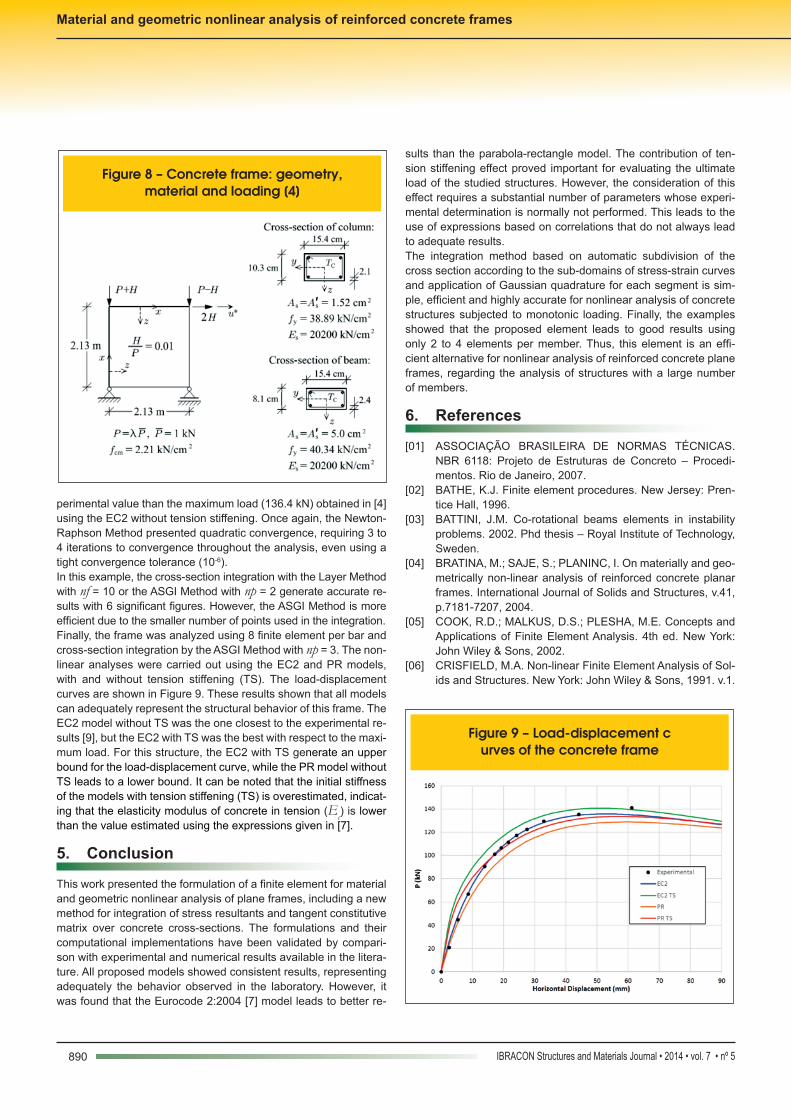
perimental value than the maximum load (136.4 kN) obtained in [4] using the EC2 without tension stiffening. Once again, the Newton-Raphson Method presented quadratic convergence, requiring 3 to 4 iterations to convergence throughout the analysis, even using a tight convergence tolerance (10-6). In this example, the cross-section integration with the Layer Method with nf = 10 or the ASGI Method with np = 2 generate accurate re-sults with 6 significant figures. However, the ASGI Method is more efficient due to the smaller number of points used in the integration. Finally, the frame was analyzed using 8 finite element per bar and cross-section integration by the ASGI Method with np = 3. The non-linear analyses were carried out using the EC2 and PR models, with and without tension stiffening (TS). The load-displacement curves are shown in Figure 9. These results shown that all models can adequately represent the structural behavior of this frame. The EC2 model without TS was the one closest to the experimental re-sults [9], but the EC2 with TS was the best with respect to the maxi-mum load. For this structure, the EC2 with TS generate an upper bound for the load-displacement curve, while the PR model without TS leads to a lower bound. It can be noted that the initial stiffness of the models with tension stiffening (TS) is overestimated, indicat-ing that the elasticity modulus of concrete in tension (Ec) is lower than the value estimated using the expressions given in [7].

5. Conclusion

This work presented the formulation of a finite element for material and geometric nonlinear analysis of plane frames, including a new method for integration of stress resultants and tangent constitutive matrix over concrete cross-sections. The formulations and their computational implementations have been validated by compari-son with experimental and numerical results available in the litera-ture. All proposed models showed consistent results, representing adequately the behavior observed in the laboratory. However, it was found that the Eurocode 2:2004 [7] model leads to better re-

Figure 8 – Concrete frame: geometry, material and loading [4]

Figure 9 – Load-displacement curves of the concrete frame

sults than the parabola-rectangle model. The contribution of ten-sion stiffening effect proved important for evaluating the ultimate load of the studied structures. However, the consideration of this effect requires a substantial number of parameters whose experi-mental determination is normally not performed. This leads to the use of expressions based on correlations that do not always lead to adequate results.The integration method based on automatic subdivision of the cross section according to the sub-domains of stress-strain curves and application of Gaussian quadrature for each segment is sim-ple, efficient and highly accurate for nonlinear analysis of concrete structures subjected to monotonic loading. Finally, the examples showed that the proposed element leads to good results using only 2 to 4 elements per member. Thus, this element is an effi-cient alternative for nonlinear analysis of reinforced concrete plane frames, regarding the analysis of structures with a large number of members.

6. References

[01] ASSOCIAÇÃO BRASILEIRA DE NORMAS TÉCNICAS. NBR 6118: Projeto de Estruturas de Concreto – Procedi-mentos. Rio de Janeiro, 2007.

[02] BATHE, K.J. Finite element procedures. New Jersey: Pren-tice Hall, 1996.

[03] BATTINI, J.M. Co-rotational beams elements in instability problems. 2002. Phd thesis – Royal Institute of Technology, Sweden.

[04] BRATINA, M.; SAJE, S.; PLANINC, I. On materially and geo-metrically non-linear analysis of reinforced concrete planar frames. International Journal of Solids and Structures, v.41, p.7181-7207, 2004.

[05] COOK, R.D.; MALKUS, D.S.; PLESHA, M.E. Concepts and Applications of Finite Element Analysis. 4th ed. New York: John Wiley & Sons, 2002.

[06] CRISFIELD, M.A. Non-linear Finite Element Analysis of Sol-ids and Structures. New York: John Wiley & Sons, 1991. v.1.



[07] EUROPEAN COMMITTEE FOR STANDARDIZATION (CEN). Eurocode 2: Design of concrete structures - Part 1-1: General rules and rules for buildings. EN 1992-1-1. Brus-sels, 2004.

[08] ESPION, B. Benchmark examples for creep and shrinkage analysis computer programs: creep and shrinkage of con-crete. TC 114 RILEM. E&FN Spon, 1993.

[09] FERGUSON, P.M.; BREEN, J.E. Investigation of the long concrete column in a frame subjected to lateral loads. Sym-posium on Reinforced Concrete Columns. American Con-crete Institute SP-13, 1966.

[10] HERNÁNDEZ-MONTES, E.; CESETTI, A.; GIL-MARTÍN, L.M. Discussion of “An efficient tension-stiffening model for nonlinear analysis of reinforced concrete members”, by Re-nata S.B. Stramandinoli, Henriette L. La Rovere, Engineer-ing Structures, v. 48, p. 763–764, 2013.

[11] MENIN, R.C.G.; TRAUTWEIN, L.M.; BITTENCOURT, T.N. Modelos de fissuração distribuída em vigas de concreto ar-mado pelo método dos elementos finitos. Revista IBRACON de Estruturas e Materiais, v.2, n.2, p.166-200, 2009.

[12] MELO, A. M. C. de Projeto ótimo de pórticos planos de con-creto armado. 2000. Tese (Doutorado em Engenharia Civil) – Universidade Federal do Rio de Janeiro, Rio de Janeiro, 2000.

[13] NANAKORN, P.; VU, L.N. A 2D field-consistent beam ele-ment for large displacement analysis using the total La-grangian formulation. Finite Elements in Analysis and De-sign, v.42, p.14-15, 2006.

[14] SPACONE, E.; FILIPPOU, F.C.; TAUCER, F.F. Fibre beam-column model for non-linear analysis of R/C frames: Part I. Formulation. Earthquake Engineering and Structural Dy-namics, v.25, p.711-725, 1996.

[15] SOUSA JR., J.B.M.; MUNIZ, C.F.D.G. Analytical integration of cross section properties for numerical analysis of rein-forced concrete, steel and composite frames. Engineering Structures, v. 29 p. 618–625, 2007.

[16] STRAMANDINOLI, R.S.B. Modelos de elementos finitos para análise não linear física e geométrica de vigas e pórti-cos planos de concreto armado. 2007. Tese (Doutorado em Engenharia Civil) – Universidade Federal de Santa Catarina, Florianópolis, 2007.

[17] STRAMANDINOLI, R.S.B.; LA ROVERE, H.L. An efficient tension-stiffening model for nonlinear analysis of reinforced concrete members, Engineering Structures, v. 30, p. 2069–2080, 2008.

Documents

Material and geometric nonlinear analysis of reinforced ... · 880 IBRACON Structures and Materials Journal • 2014 • vol. 7 • n 5 Material and geometric nonlinear analysis of