Embed Size (px)
Citation preview
ISSN 0351-336X
SOJUZNA MATEMATIQARITE
NA R. MAKEDONIJA
MATEMATIQKI BILTEN
BULLETIN MATHEMATIQUE
KNIGA 39 (LXV) TOME
No. 2
REDAKCISKI ODBOR
Malqeski Aleksa (Makedonija)
Markoski Gorgi - Sekretar
Balan Vladimir (Romanija)
Coban Mitrofan (Moldavija)
Felloris Argyris (Grcija)
Manova-Erakovik Vesna (Makedonija)
Mushkarov Oleg (Bugarija)
Oberguggenberger Michael (Avstrija)
Pilipovic Stevan (Srbija)
Scarpalezos Dimitrios (Francija)
Skrekovski Riste (Slovenija)
Valov Vesko (Kanada)
Vindas Jasson (Belgija)
COMITE DE REDACTION
Malcheski Aleksa (Macedoine)
Markoski Gorgi - Secretaire
Balan Vladimir (Roumanie)
Coban Mitrofan (Moldavie)
Felloris Argyris (Grece)
Manova-Erakovic Vesna (Macedoine)
Mushkarov Oleg (Bugarie)
Oberguggenberger Michael (Autriche)
Pilipovic Stevan (Serbie)
Scarpalezos Dimitrios (France)
Skrekovski Riste (Slovenie)
Valov Vesko (Canada)
Vindas Jasson (Belgique)
SKOPJE – SKOPJE2015
2
MATEMATIQKI BILTEN e naslednik na BILTENOT NA DRUXTVOTONA MATEMATIQARITE I FIZIQARITE NA MAKEDONIJA. Se peqatiod 1950 godina. Objavuva originalni nauqni trudovi od site oblasti na mate-matikata i nejzinite primeni, na makedonski jazik ili na eden od svetskitejazici: angliski, francuski, germanski ili ruski. Izleguva dvapati godixno.Indeksiran e vo Mathematical Reviews (MathSciNet), Zentralblatt Math i Refera-tivnyi Zhurnal (VINITI).
Poelno e trudot da bide napixan vo nekoja verzija na LaTex (no moe ivo WORD) i da ne bide pogolem od deset stranici. Trudot se dostavuva voelektronska forma na sledniov
e-mail: [email protected]
Sekoja statija treba da ima apstrakt, glaven del i rezime. Ako statijata enapixana na makedonski jazik, togax rezimeto treba da bide na angliski jazik,ako, pak, statijata e napixana na eden od svetskite jazici, togax rezimeto trebada bide na makedonski jazik. Vo poqetna faza trudovite moe da se dostavat ivo peqatena verzija, vo dva primeroka, na slednava adresa:
MATEMATIQKI BILTEN
Sojuz na matematiqari na Makedonija
Bul. Aleksandar Makedonski, bb
P. Fah 10, 1000 Skopje
R. Makedonija
MATEMATICKI BILTEN - BULLETIN MATHEMATIQUE is a successor of the BIL-TEN NA DRUSTVOTO NA MATEMATICARITE I FIZICARITE NA MAKEDONIJA.It is published since 1950. It publishes original papers of all branches of mathematicsand its applications. Papers can be written in Macedonian or in one of the following lan-guages: English, French, Russian or German. Frequency: twice a year. MATEMATICKIBILTEN is covered by the following services: Mathematical Reviews (MathSciNet), Zen-tralblatt fr Mathematik and Referativnyi Zhurnal (VINITI).
Papers should be written preferably in some version of LaTex (or MS Word) and shouldnot exceed ten pages. They should be submitted in electronic form to the following
e-mail: [email protected]
Every paper should contain abstract, main part and summary. If the paper is written inMacedonian, then summary should be written in English and if the paper is written in oneof the above mentioned languages, then the summary should be written in Macedonianlanguage. In the initial phase the papers can be submitted in two copies in printedversion as well, to the following address:
MATEMATICKI BILTEN
Union of Mathematicians of Macedonia
Blvd. Aleksandar Makedonski, bb
P.O. Box 10, 1000 Skopje
Republic of Macedonia
∗ ∗ ∗Izdavanjeto na Matematiqkiot bilten go finansira
Ministerstvoto za obrazovanie i nauka
Matematiqki Bilten ISSN 0351-336XVol.38 (LXIV) No.22014 (3)Skopje, Makedonija
SODRINA
1. Dragan S. DjordjevicREVERSE ORDER LAW FOR THE MOORE-PENROSEINVERSE OF CLOSED-RANGE ADJOINTABLE OPERATORSON HILBERT C*-MODULES . . . . . . . . . . . . . . . . . . . . . . . . . . . . . . . . . . . . . . . . 5
2. Jitka LaitochovaALGEBRAIC MODEL OF DIFFERENCE EQUATIONS ANDFUNCTIONAL EQUATIONS . . . . . . . . . . . . . . . . . . . . . . . . . . . . . . . . . . . . . . . 13
3. Miroslav S. Petrov and Todor D. TodorovBARZILAI-BORWEIN METHOD FOR A NONLOCALELLIPTIC PROBLEM . . . . . . . . . . . . . . . . . . . . . . . . . . . . . . . . . . . . . . . . . . . . . . 23
4. Andrea Aglic Aljinovic, Josip Pecaric and Anamarija Perusic PribanicGENERALIZATIONS OF STEFFENSEN’S INEQUALITYVIA n WEIGHT FUNCTIONS . . . . . . . . . . . . . . . . . . . . . . . . . . . . . . . . . . . . . . 31
5. Julije Jaksetic, Josip Pecaric and Anamarija PerusicGENERALIZATIONS OF STEFFENSENS INEQUALITYBY HERMITES POLYNOMIAL . . . . . . . . . . . . . . . . . . . . . . . . . . . . . . . . . . . . .53
6. Milica Klaricic Bakula, Josip Pecaric,Mihaela Ribicic Penava and Ana VukelicSOME INEQUALITIES FOR THE EBYEV FUNCTIONAL ANDGENERAL FOUR-POINT QUADRATURE FORMULAEOF EULER TYPE . . . . . . . . . . . . . . . . . . . . . . . . . . . . . . . . . . . . . . . . . . . . . . . . . . 69
7. Josip Pecaric and Ksenija Smoljak KalamirGAUSS-STEFFENSEN TYPE INEQUALITIES . . . . . . . . . . . . . . . . . . . . . 81
8. Qiulan Qi and Ge YangMODIFIED BASKAKOV-KANTOROVICH OPERATORSPROVIDING A BETTER ERROR ESTIMATION . . . . . . . . . . . . . . . . . . 91

Matematiqki Bilten ISSN 0351-336XVol.38 (LXIV) No.22014 (5–11) UDC: 515.142.32Skopje, Makedonija
REVERSE ORDER LAW FOR THE MOORE-PENROSEINVERSE OF CLOSED-RANGE ADJOINTABLE OPERATORS
ON HILBERT C∗-MODULES
DRAGAN S. DJORDJEVIĆ
Abstract. Results related to bounded andjointable operators on Hilbert C∗-modules are presented. Results concerning generalized inverses are included.
1. Introduction
Let A be a complex C∗-algebra with the norm ‖ · ‖, and let M be a complexlinear space. M is a (right) A-module, provided that there exists an exteriormultiplication · :M×A→M, obeying the following properties, for all x, y ∈M,all a, b ∈ A and all λ ∈ C:
(x+ y) · a = x · a+ y · a; x · (a+ b) = x · a+ y · b;x · (ab) = (x · a) · b; λ(xa) = (λx)a = x(λa).
If M is an A-module, then the A-valued inner product is the function 〈·, ·〉 :M×M→ A, satisfying the following conditions, for all x, y ∈M, all a ∈ A:〈x, x〉 ≥ 0 in A; x = 0 if and only if 〈x, x〉 = 0;〈x, y〉 = 〈y, x〉∗; 〈x, λy + µz〉 = λ〈x, y〉+ µ〈x, z〉;〈x, y · a〉 = 〈x, y〉a.Thus,M becomes a pre-Hilbert A-module.The norm on a pre-Hilbert A-moduleM is defined by ‖x‖M = ‖〈x, x〉‖1/2. This
norm satisfies some nice properties, which are related to the Cauchy-Bunyakovsky-Schwarz inequality:〈x, y〉〈y, x〉 ≤ ‖y‖2M 〈x, x〉, for all x, y ∈M;‖x · a‖M ≤ ‖x‖M ‖a‖, for all x ∈M and all a ∈ A;‖〈x, y〉‖ ≤ ‖x‖M‖y‖M for all x, y ∈M.Finally, ifM is a Banach space with respect to the norm ‖ · ‖M, thenM is a
Hilbert A-module. We also say thatM is a Hilbert C∗-module (over A). If H is acomplex Hilbert space, then H is a Hilbert C-module. Hence, Hilbert C∗-modulesare between Hilbert spaces and Banach spaces.
2010 Mathematics Subject Classification. 46L08.Key words and phrases. Moore-Penrose inverse; reverse order law; adjointable operators;
Hilbert C∗-modules.5
6 DRAGAN S. DJORDJEVIĆ
LetM,N be Hilbert A-modules, and let T :M→ N be a linear mapping. Tis an operator, if T is bounded (as an operator between Banach spaces) and T isA-linear, i.e. T (x · a) = T (x) · a for all x ∈M and all a ∈ A.
If T is an operator fromM to N , and there exists an operator T ∗ from N toM satisfying 〈Tx, y〉 = 〈x, T ∗y〉 for all x ∈ M and all y ∈ N , them T ∗ is theadjoint of T , and T is adjointable. Notice that there exist operators which are notadjointable. We use Hom∗(M,N ) to denote the set of all adjointable operatorsfromM to N . Recall that End∗(M) = Hom∗(M,M) is a C∗-algebra.
If T ∈ Hom∗(M,N ), then R(T ) denote the range of T , and N (T ) denote thekernel of T . Notice that N (T ) is always closed.
Among the situation that there exists non-adjointable operators between HilbertA-modules, there also is the following non-convenient situation. Let K be a closedsubmodule ofM. The orthogonal complement of K is defined as K⊥ = x ∈M :〈x, y〉 = 0 for all y ∈ K. Although K⊥ is a closed submodule of M, we do nothave in generalM = K ⊕K⊥.
However, in the case which is the most important for this research, we have thefollowing result.
Theorem 1. ([9], [10]) LetM,N be a Hilbert A-modules, and let T ∈ Hom∗(M,N ).If R(T ) is closed, then the following hold:N (T ) is an orthogonally complemented submodule inM andM = R(T ∗)⊕N (T );R(T ) is an orthogonally complemented submodule in N and N = R(T )⊕N (T ∗).
Previous result allows us to investigate adjointable operators between HilbertA-modules in a similar way as on Hilbert spaces. For detailed treatment of HilbertC∗-modules see [9] and [10].
Now, we have the usual definition of the Moore-Penrose inverse. Let T ∈Hom∗(M,N ). The operator T † ∈ Hom∗(M,N ) is the Moore-Penrose inverse ofT , provided that the following holds:
TT †T = T, T †TT † = T †, (TT †)∗ = TT †, (T †T )∗ = T †T.
The Moore-Penrose inverse is unique in the case when it exists: this is standardfor all standard structures that admits the existence of the Moore-Penrose inverse.Moreover, T † exists if and only if R(T ) is closed in N (see [14]).
In this paper we are interested in the reverse order law for the Moore-Penroseinverse. If a, b are invertible elements in an unital semigroup, then (ab)−1 = b−1a−1
is the reverse order law for the ordinary inverse. However, the rule (ab)† = b†a†
does not hold in general for the Moore-Penrose inverse. If a, b are Moore-Penroseinvertible, then it does not follows that ab is also Moore-Penrose invertible. Sincewe consider only Hilbert modules, we refer to the result which explain when theproduct of two closed-range adjointalbe operators also has a closed range. Oneequivalent condition is proved in [12].
In this paper we prove some equivalencies of the reverse order rule (AB)† =B†A†, where A,B,AB are adjointable operators between Hilbert modules, that
REVERSE ORDER LAW FOR THE MOORE-PENROSE INVERSE... 7
have closed ranges. This result is known in the case of bounded Hilbert space op-erators, and in some parts in rings with involutions. We demostrate the usefulnessof Theorem 1 for the geometric theory of generalized inverse.
Let T ∈ Hom∗(M, N) has a closed range. Then T †T is the orthogonal projec-tion fromM ontoR(T ∗), and TT † is the orthogonal projection fromN ontoR(T ).Using these projections, we see that T has the following matrix decomposition:
T =
[T1 00 0
]:
[R(T ∗)N (T )
]→
[R(T )N (T ∗)
].
The operator T1 is invertible and adjointable, so
T † =
[T−11 00 0
]:
[R(T )N (T ∗)
]→
[R(T ∗)N (T )
].
This decomposition allows us to reduce some properties of non-invertible T toinvertible T1.
Previous representation is derived from block representations of operators onBanach and Hilbert spaces, as well as Hilbert C∗-modules (see, for example, [4],[6], [12], [13]). This representation, and derived ones, are systematically used inthe investigation of generalized inverses.
Let T ∈ Hom∗(M,N ) have a closed range. T is EP if and only if TT † = T †T .Equivalently, T is EP if and only if R(T ) = R(T ∗) (see [12] for EP operatorson Hilbert modules). Obviously, T is EP if and only if T ∗ is EP. Notice thatselfadjoint and normal operators with closed range are EP operators.
We use [T, S] = TS − ST to denote the commutator of operators T and S. Inthis paper we use the fact that if T and S are selfadjoint, then TS is selfadjoint ifand only if [T, S] = 0.
2. Results
We prove the following main result of this paper.
Theorem 2. Let A be a C∗-algebra, and letM,N ,K be Hilbert A-modules. Sup-pose that A ∈ Hom∗(N ,K), B ∈ Hom∗(M,N ) be adjointable operators, such thatA,B,AB have closed ranges. Then the following statements are equivalent:
(a) (AB)† = B†A†;(b) [A†A,BB∗] = 0 and [A∗A,BB†] = 0;(c) R(A∗AB) ⊂ R(B) and R(BB∗A∗) ⊂ R(A∗);(d) A∗ABB∗ is EP.
Proof. Using previous ideas, we know that A =
[A1 00 0
]:
[R(A∗)N (A)
]→
[R(A)N (A∗)
],
where A1 is invertible, and consequently A† =[A−11 00 0
]. Also, B =
[B1 0B2 0
]:[
R(B∗)N (B)
]→
[R(A∗)N (A)
]. Notice that D = B∗1B1 + B∗2B2 is positive and invertible
in End∗(R(B∗)). Hence, B† = (B∗B)†B∗ =
[D−1B∗1 D−1B∗2
0 0
].
8 DRAGAN S. DJORDJEVIĆ
We find equivalent forms of (a). Notice that AB =
[A1B1 00 0
]and B†A† =[
D−1B∗1A−11 0
0 0
]. Hence, (AB)† = B†A† if and only if (A1B1)
† = D−1B∗1A−11 .
We have the following: A1B1(D−1B∗1A
−11 )A1B1 = A1B1 if and only if
B1D−1B∗1B1 = B1. (2.1)
Also, D−1B∗1A−11 (A1B1)D
−1B∗1A−11 = D−1B∗1A
−11 if and only if (2.1) holds. The
operator A1B1D−1B∗1A
−11 is Hermitian if and only if
[A∗1A1, B1D−1B∗1 ] = 0. (2.2)
Finally, D−1B∗1A−11 A1B1 is Hermitian if and only if
[D,B∗1B1] = 0. (2.3)
Now we find equivalent forms of (b). We haveA†A =
[I 00 0
], A∗A =
[A∗1A1 00 0
],
BB∗ =
[B1B
∗1 B1B
∗2
B2B∗1 B2B
∗2
]andBB† =
[B1D
−1B∗1 B1D−1B∗2
B2D−1B∗1 B2D
−1B∗2
]. Hence, [A†A,BB∗] =
0 if and only ifB1B
∗2 = 0. (2.4)
Also, [A∗A,BB†] = 0 if and olny if
[A∗1A1, B1D−1B∗1 ] = 0 (2.5)
andB2D
−1B∗1 = 0. (2.6)We find equivalent conditions for (c). Notice that R(A∗AB) ⊂ R(B) holds
if and only if BB†A∗AB = A∗AB. Also, R(BB∗A∗) ⊂ R(A∗) if and only ifA†ABB∗A∗ = BB∗A∗. From previous decompositions of operators we see thatA†ABB∗A∗ = BB∗A∗ if and only if
B2B∗1 = 0, (2.7)
which the same as (2.4). We have BB†A∗AB = A∗AB if and only if
B1D−1B∗1A
∗1A1B1 = A∗1A1B1 (2.8)
andB2D
−1B∗1A∗1A1B1 = 0. (2.9)
Thus, (c) is equivalent to (2.7), (2.8) i (2.9).Finally, (d) is equivalent to
R(A∗ABB∗) = R(BB∗A∗A), (2.10)
assuming that this submodule is closed.(b) =⇒ (a): We prove the following:(
(2.4) ∧ (2.5) ∧ (2.6))
=⇒((2.1) ∧ (2.2) ∧ (2.3)
).
REVERSE ORDER LAW FOR THE MOORE-PENROSE INVERSE... 9
Suppose that (2.4), (2.5) and (2.6) hold. Obviously, (2.2) holds. Also,
B∗1 = DD−1B∗1 = (B∗1B1 +B∗2B2)D−1B∗1 = B∗1B1D
−1B∗1 .
Thus, (2.1) holds. We see that B∗1B1D−1B∗1B1 = B∗1B1 is satisfied, so R(B∗1B1)
is closed. We have the following matrix form of B∗1B1: B∗1B1 =
[C1 00 0
]:[
R(B∗1B1)N (B∗1B1)
]→
[R(B∗1B1)N (B∗1B1)
]. Since R(B∗2B2) ⊂ N (B∗1B1) we have B∗2B2 =[
0 0C3 C4
]:
[R(B∗1B1)N (B∗1B1)
]→
[R(B∗1B1)N (B∗1B1)
]. However, B∗2B2 is Hermitian, so C3 = 0.
Thus, D =
[C1 00 C4
]and it obviously commutes with B∗1B1. Thus, (2.3) holds.
(a) =⇒ (b): We prove((1) ∧ (2) ∧ (3)
)=⇒
((4) ∧ (5) ∧ (6)
).
Suppose that (1), (2) and (3) hold. Since D commutes with B∗1B1, we get thatD−1 commute with B∗1B1. Hence, we get
B1 = B1D−1B∗1B1 = B1(D −B∗2B2)D
−1 = B1 −B∗2B2D−1.
It follows that B1B∗2B2 = 0. Since R(B∗2) = R(B∗2B2) and R(B∗2B2) ⊂ N (B1), we
get R(B∗2) ⊂ N (B1), so B1B∗2 = 0. Thus, (4) is proved. Also, (5) is obvious. From
B1B∗2 = 0 we get B∗1B1B
∗2 = 0 and B∗1B1D
−1B∗2 = 0. Hence, B2D−1B∗1B1 = 0.
In the same manner as before, we conclude that B2D−1B∗1 = 0, so (6) holds.
(a)∧(b) =⇒ (c): It is enough to observe the following elementary implications:
(5) ∧ (1) =⇒ (8), (4) ⇐⇒ (7), (6) =⇒ (9).
(c) =⇒ (b): We prove the implication:((7) ∧ (8) ∧ (9)
)=⇒
((4) ∧ (5) ∧ (6)
).
Obviously, (7)⇐⇒ (4). From (9) we getR(B∗1A∗1) = R(B∗1A∗1A1B1) ⊂ N (B2D−1),
implying that B2D−1B∗1A
∗1 = 0, so (6) follows. We multiply (8) by (A1B1)
†
and use the equality G∗GG† = G∗ whenever G is Moore-Penrose invertible.Hence, we get B1D
−1B∗1A∗1 = A∗1A1B1(A1B1)
†, implying that B1D−1B∗1A
∗1A1 =
A∗1(A1B1(A1B1)†)A1. We know that A1B1(A1B1)
† is selfadjoint, and thereforeA∗1(A1B1(A1B1)
†)A1 is selfadjoint. Now, B1D−1B∗1A
∗1A1 is selfadjoint.
Since both B1D−1B∗1 and A∗1A1 are selfadjoint, we get
[B1D−1B∗1 , A
∗1A1] = 0,
so (5) follows.(d) =⇒ (c): Let A∗ABB∗ be EP. Then we have
R(A∗AB) = R(A∗ABB∗) = R(BB∗A∗A) ⊂ R(B)
andR(BB∗A∗) = R(BB∗A∗A) = R(A∗ABB∗) ⊂ R(A∗).
Hence, (c) holds.
10 DRAGAN S. DJORDJEVIĆ
(c) =⇒ (d): Suppose that all conditions (7),(8),(9) hold. We find the equivalentform of (10). Under these assumptions, we have that (10) is equivalent to
R([A∗1A1B1B
∗1 A∗1A1B
∗1B2
0 0
])=
([B1B
∗1A∗1 0
B2B∗1A∗1A1 0
]).
Since (7) holds, we see that (1) is equivalent to
R(A∗1A1B1B∗1) = R(B1B
∗1A∗1A1).
The operator A1 is invertible, so the last equality is equivalent to
R(A∗1A1B1B∗1) = R(B1B
∗1).
Using the closed-range assumptions, the last one is equivalent to
R(A∗1A1B1) = R(B1),
which is the same asB1B
†1A∗1A1B1 = A∗1A1B1. (2.11)
Now we start from (8) and obtain the following:
B1B†1A∗1A1B1 = B1B
†1B1D
−1B∗1A∗1A1B1 = B1D
−1B∗1A∗1A1B1 = A∗1A1B1.
Thus, (8) implies (11). Hence, we have just proved that (c) implies (d).
This theorem represents an extension of well-know results for matrices andoperators on Hilbert spaces (see [1], [2], [3], [7], [8]) to the more general settings:we considered the Moore-Penrose inverse of a product of closed-range adjointableoperators on Hilbert C∗-modules. See also [5] and [11] for some algebraic aspects.
References
[1] A. Ben-Israel, T. N. E. Greville, Generalized inverses: theory and applications, 2nded., Springer, New York, 2003.
[2] R. H. Bouldin, The pseudo-inverse of a product, SIAM J. Appl. Math. 25 (1973), 489–495.
[3] R. H. Bouldin, Generalized inverses and factorizations, Recent Applications of Gener-alized Inverses, Pitman Ser. Res. Notes in Math. No. 66 (1982), 233–248.
[4] D. S. Djordjević, Unified approach to the reverse order rule for generalized inverses,Acta Sci. Math. (Szeged) 67 (2001), 761–776.
[5] J. J. Koliha, D. S. Djordjević, D. Cvetković Ilić, Moore–Penrose inverse in rings withinvolution, Linear Algebra Appl. 426 (2007) 371–381.
[6] D. S. Djordjević and N. Č. Dinčić, Reverse order law for the Moore-Penrose inverse,J. Math. Anal. Appl. 361 (2010), 252–261.
[7] T. N. E. Greville, Note on the generalized inverse of a matrix product, SIAM Rev. 8(1966), 518–521.
[8] S. Izumino, The product of operators with closed range and an extension of the reverseorder law, Tohoku Math. J. 34 (1982), 43–52.
[9] E. C. Lance, Hilbert C∗-modules – a toolkit for operator algebraists, Cambridge Uni-versity Press, Cambridge-New York-Melbourne, 1995.
[10] V. M. Manuilov, E. V. Troitsky, Hilbert C∗-modules, Translations of MathematicalMonographs, American Mathematical Society, Providence, Rhode Island, 2005.
[11] D. Mosić, D. S. Djordjević, Reverse order laws in rings with involution, Rocky Moun-tain J. Math. 44 (4) (2014), 1301–1319.
REVERSE ORDER LAW FOR THE MOORE-PENROSE INVERSE... 11
[12] K. Sharifi, The product of operators with closed range in Hilbert C∗-modules, LinearAlgebra Appl. 435 (2011), 1122–1130.
[13] K. Sharifi, EP modular operators and their products, J. Math. Anal. Appl. 419 (2014),870–877.
[14] Q. Xu, L. Sheng, Positive semi-definite matrices of adjointable operators on HilbertC∗-modules, Linear Algebra Appl. 428 (2008), 992–1000.
University of Niš, Faculty of Sciences and Mathematics,Višegradska 33, 18000 Niš, SerbiaE-mail address: [email protected], [email protected]

Matematiqki Bilten ISSN 0351-336XVol.38 (LXIV) No.22014 (13–21) UDC: 517.9:515.178.2Skopje, Makedonija
ALGEBRAIC MODEL OF DIFFERENCE EQUATIONSAND FUNCTIONAL EQUATIONS
JITKA LAITOCHOVÁ
Abstract. We will deal with the theory of Abel functional equations in thespace of strictly monotonic functions S. The Abel functional equation modelreduces under specialization to a linear functional or to a linear differenceequation. Definitions, structure, and general theory for Abel functional equa-tions on S appear. The approach duplicates a rich body of known definitions,results and properties for classical functional and difference equations.
The setting for the algebraic model is in the space S of strictly monotonicreal functions f defined on the interval J = (−∞,∞). It is required thatf map J one-to-one onto an interval (a, b), where a and b are extended realnumbers.
The model equation is expressed in terms of iteration of a function Φ in S.The iteration process uses a canonical function in S, which is an arbitrarilychosen increasing function X ∈ S.
A method is presented for solving the new model equation. This methodcan be applied to solve, in particular, some classical linear functional anddifference equations.
1. Introduction
We will deal with the theory of Abel functional equations in the space of strictlymonotonic functions. The first known model, introduced by O. Bor uvka [1], is spe-cific to differential equations, whereas the model we introduce is independent ofdifferential equations. The Abel functional equation model reduces under special-ization to a linear functional or a difference equation. The approach duplicates arich body of known definitions, results and properties for classical functional anddifference equations [3], [2], [8].
The setting for the algebraic model is in the space S of strictly monotonic realfunctions f defined on the interval J = (−∞,∞). It is required that f map Jone-to-one onto an interval (a, b), where a and b are real or extended numbers.
The model equation is expressed in terms of iteration of a function Φ in S. Theiteration process uses a canonical function in S, which is an arbitrarily chosenincreasing function X ∈ S.
2010 Mathematics Subject Classification. 39B05; 39B12.Key words and phrases. Linear kth order functional equation, linear kth order difference
equation, space of continuous strictly monotonic functions, group multiplication, generalizedAbel functional equation.
13
14 JITKA LAITOCHOVÁ
The function Φ is algebraically a phase function known from Borùvka’s theoryof linear differential transformations of the second order [1]. The theory is usefulfor investigating oscillatory and asymptotic properties of solutions of ordinarylinear differential equations. By a phase function, Bor uvka meant a function αdefined in an open interval j such that α ∈ C1, α′ 6= 0 for all t ∈ j. Each phasefunction α ∈ C3 represents, in its domain j, a first phase of the differential equationy′′ = q(t)y, where the first phase is any continuous function α defined on j whichsatisfies tanα(t) = u(t)
v(t) except at zeros of v, and (u, v) is a solution basis of theequation.
A method is presented for solving the new model equation. This method canbe applied to solve, in particular, some classical linear functional and differenceequations.
Because difference equation theory uses the difference operator to express cer-tain results, the notion of a difference operator is defined for Abel functional equa-tions on S. Results are obtained for difference and sum operators, which reduce,when the model equation is a difference equation, to classical known results.
A solution of the linear functional equation is considered to be a continuousfunction f on an interval 〈x0,∞). A solution f of the difference equation isconsidered on a sequence of points xn∞0 .
If domains of coefficients and right sides of the equations are considered to bethe interval J , which is the union of intervals jµ = (xµ, xµ+1), µ = −∞ to ∞,then solutions of linear functional equations are continuous functions on J whilesolutions of linear difference equations are two-sided sequences xn∞n=−∞. Thedefinition of symbol xn appears below.
Algebraic models directly related to α(f(x)) = α(x) + 1, which is the classicalAbel functional equation, are studied in [5]. The new models are treated abstractlyas the (generalized) Abel functional equation α(f(x)) = g(α(x)), in which f and gare given and α is the unknown. Given an increasing function f , possibly havingfixed points in its domain (a, b), a group-theoretic iterative explicit constructionis given for infinitely many solutions α which are infinite at fixed points of fand otherwise monotonic. The group-theoretic structure is suitable for studyingsolution properties of Abel functional equations. The methods apply in particularto Abel functional equations for which the domain (a, b) is a finite interval, a half-line or the real line. The function f is allowed to have many fixed points x, definedby the equation f(x) = X(x), where X(x) is a canonical function in S (X(x) = xgives classical fixed points).
It is shown how to form an Abel functional equation which represents a lin-ear homogeneous functional equation with constant coefficients. Results of thespecialization are stated. The Abel functional equation model in S is able tosimultaneously model both k-th order linear difference equation with constantcoefficients [4] and first order linear difference equations with constant and non-constant coefficients [6]. Some applications appear, which show how to do theuniform modeling of classical equations.
ALGEBRAIC MODEL OF FUNCTIONAL EQUATIONS 15
2. Space of strictly monotonic functions
Definition 2.1: Given a, b ∈ R, a < b. The set of all continuous functions on(−∞,∞) which map one-to-one the interval (−∞,∞) onto (a, b) will be denotedby the symbol Sba and called a space of strictly monotonic functions.Definition 2.2: An arbitrarily chosen increasing function X = X(x), X ∈ S, willbe called a canonical function in S. The inverse to the canonical function Xwill be denoted by X∗.Definition 2.3: Let α, β ∈ S. The composite function γ = α(X∗(β(x))), shortlyγ = αX∗β(x), will be called a product and denoted γ = α β.Remark 2.1: The set S with the operation of multiplication forms a non-commutative group.Definition 2.4: Let φ ∈ S, φ increasing and X ∈ S be a canonical function,φ > X on (−∞,∞). The iterates of φ in S are given by
φ0(x) = X(x)
φn+1(x) = φ φn(x), n = 0, 1, 2, . . .
φn−1(x) = φ−1 φn(x), n = 0,−1,−2, . . . ,
x ∈ (−∞,∞), where φ−1 is the inverse element according to .
3. Constant-coefficient kth order equation
Consider the homogeneous constant-coefficient equation
akf φk(x) + ak−1f φk−1(x) + · · ·+ a0f φ0(x) = 0, (HCCE)
where ai ∈ R, i = 0, 1, 2, . . . , k.Functional Equation. If the x-domain is (−∞,∞), then a solution of (HCCE)
is a function f ∈ C0(−∞,∞) that satisfies the equation for all x.Difference Equation. If the x-domain is a discrete sequenceO = X∗φn(x0),
then a solution of (HCCE) is a function f defined on O which satisfies the equationat each x = X∗φn(x0).
3.1. Generalized Abel functional equation. The solution f(x) of (HCCE)will be given in terms of the generalized Abel equation
α φ(x) = g α(x).
We assume g(x) = X(x+ 1), then the Abel equation is
α φ(x) = X(x+ 1) α(x). (AFE)
Equation (AFE) is called the associated functional equation of (HCCE).Known are X and φ in S. Function α is the solution of (AFE).
16 JITKA LAITOCHOVÁ
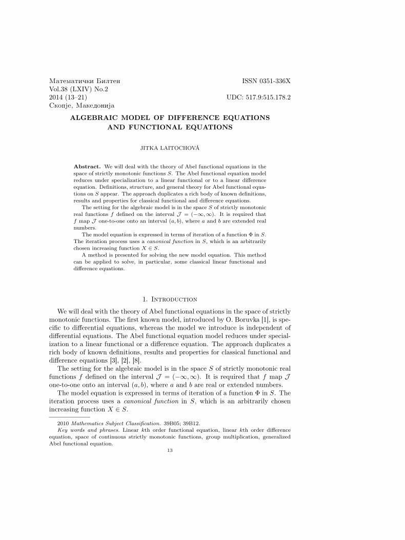
x = −7.6
x
x = 1x = −1 x = 5.4
y14
−8
Figure. An iterative solution of α(φ(x)) = α(x) + 1, where φ(x) = 11+x2 − 1
2 + x.
Example 3.1: We shall consider the specialized Abel functional equation
α(φ(x)) = α(x) + 1,
where
φ(x) =1
1 + x2− 1
2+ x.
The function φ has fixed points at x = ±1, where α is infinite. The fixed pointsseparate regions of increase of α and decrease of α. The segments of the solutionα represent the iterative steps used to produce the graphic in the preceding figure.Generally, infinitely many iterations are required to fully represent α.
For the theory of functional equations see [3]. The theory of difference equa-tions can be found in [2] and [8]. For more results on generalized Abel functionalequation and linear kth order equations in S see [4], [5], [6] and [7].
3.2. Simple positive root theorem.
Theorem 1. Let equation (HCCE) be given. Let λ1, λ2, . . . , λk be simple positiveroots of the characteristic equation
akλk + ak−1λ
k−1 + · · ·+ a1λ+ a0 = 0
Let α be a continuous solution of the associated Abel functional equation (AFE).Then the functions
f1 = λX∗α(x)1 , f2 = λ
X∗α(x)2 , . . . , fk = λ
X∗α(x)k ,
are linearly independent solutions of (HCCE).
ALGEBRAIC MODEL OF FUNCTIONAL EQUATIONS 17
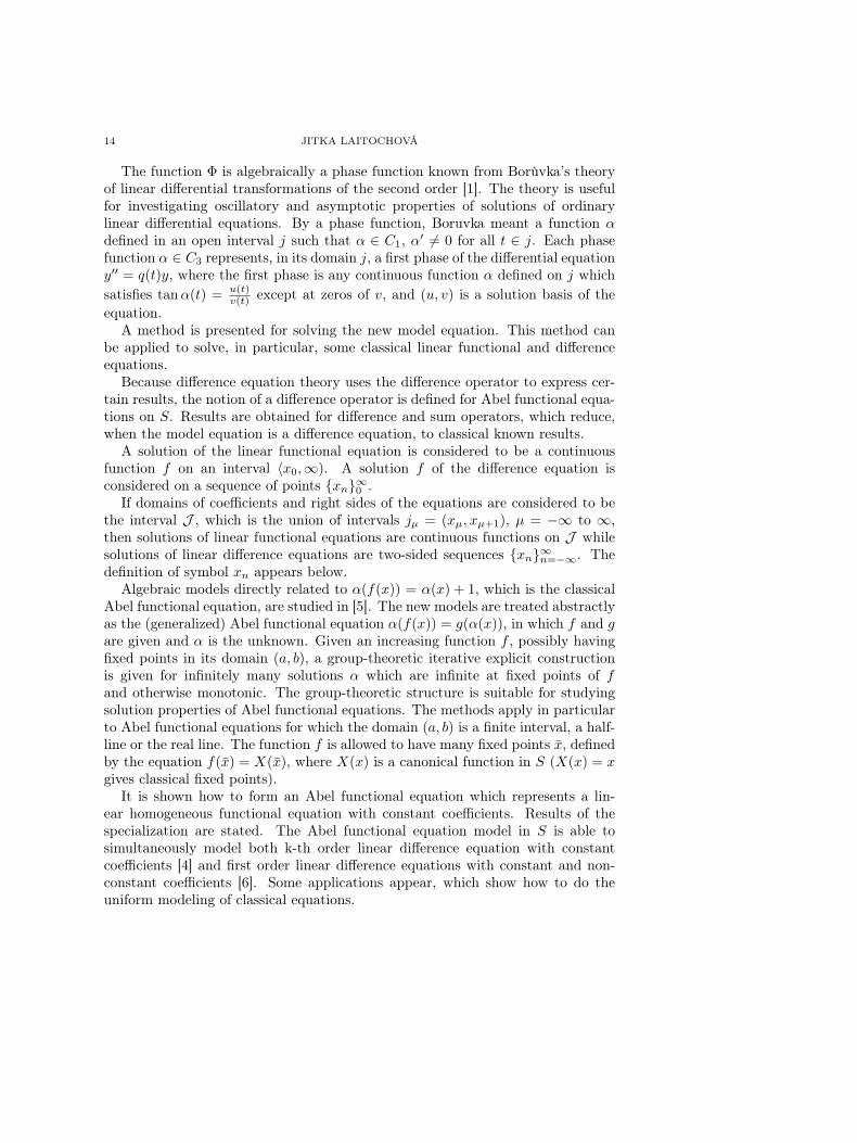
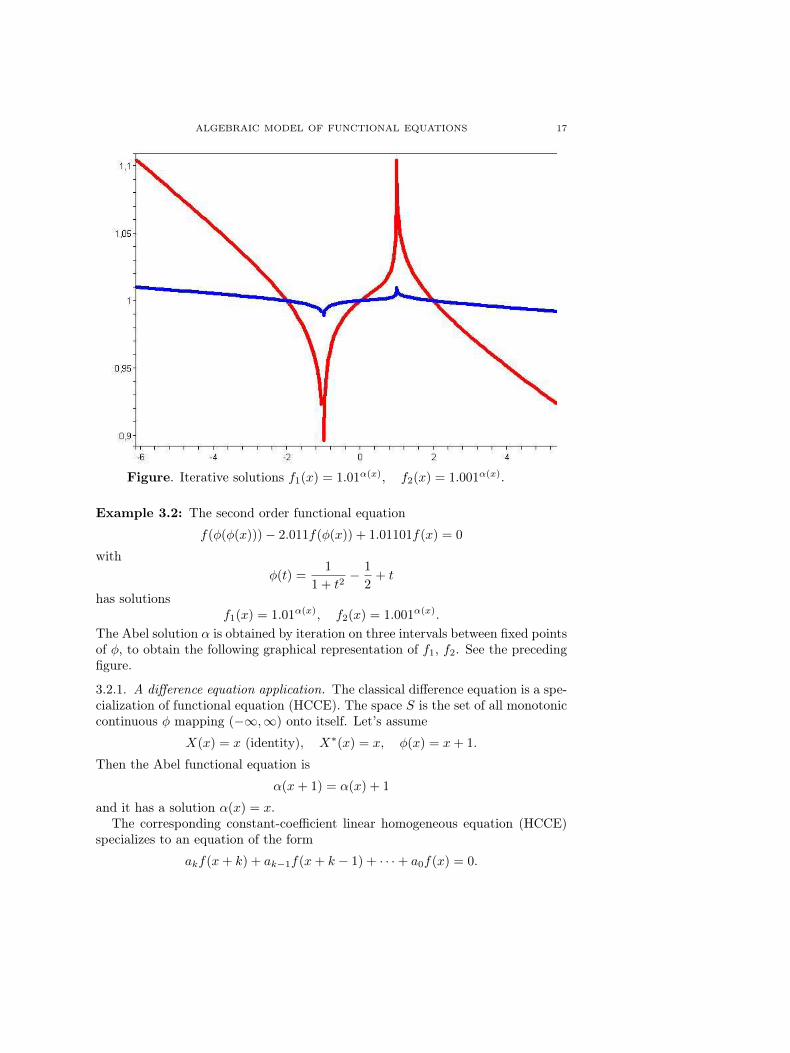
Figure. Iterative solutions f1(x) = 1.01α(x), f2(x) = 1.001α(x).
Example 3.2: The second order functional equation
f(φ(φ(x)))− 2.011f(φ(x)) + 1.01101f(x) = 0
withφ(t) =
1
1 + t2− 1
2+ t
has solutionsf1(x) = 1.01α(x), f2(x) = 1.001α(x).
The Abel solution α is obtained by iteration on three intervals between fixed pointsof φ, to obtain the following graphical representation of f1, f2. See the precedingfigure.
3.2.1. A difference equation application. The classical difference equation is a spe-cialization of functional equation (HCCE). The space S is the set of all monotoniccontinuous φ mapping (−∞,∞) onto itself. Let’s assume
X(x) = x (identity), X∗(x) = x, φ(x) = x+ 1.
Then the Abel functional equation is
α(x+ 1) = α(x) + 1
and it has a solution α(x) = x.The corresponding constant-coefficient linear homogeneous equation (HCCE)
specializes to an equation of the form
akf(x+ k) + ak−1f(x+ k − 1) + · · ·+ a0f(x) = 0.
18 JITKA LAITOCHOVÁ
If λ > 0 is a root of the characteristic equation, then a special solution isf(x) = λX
∗α(x), where α satisfies the Abel equation. Because α(x) = x andX(x) = x, then the special solution is
f(x) = λx.
3.3. Multiple positive root theorem.
Theorem 2. Let constant-coefficient equation (HCCE) be given. Let λ0 be apositive real root of the characteristic equation
akλk + ak−1λ
k−1 + · · ·+ a1λ+ a0 = 0
of multiplicity s, 1 ≤ s ≤ k. Let α(x) be a continuous solution of Abel functionalequation (AFE) and let X∗ be the inverse function to canonical function X.Then the functions
fr(x) = (X∗α(x))rλX∗α(x)0 , 0 ≤ r < s
are independent solutions of equation (HCCE).
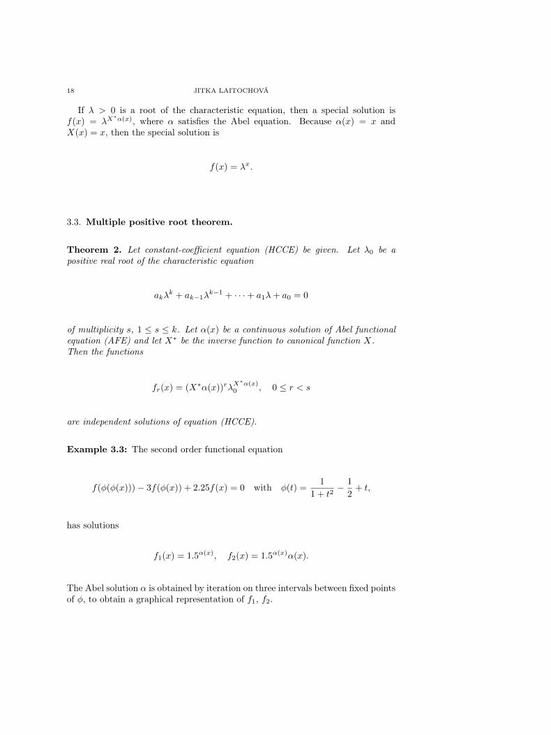
Example 3.3: The second order functional equation
f(φ(φ(x)))− 3f(φ(x)) + 2.25f(x) = 0 with φ(t) =1
1 + t2− 1
2+ t,
has solutions
f1(x) = 1.5α(x), f2(x) = 1.5α(x)α(x).
The Abel solution α is obtained by iteration on three intervals between fixed pointsof φ, to obtain a graphical representation of f1, f2.
ALGEBRAIC MODEL OF FUNCTIONAL EQUATIONS 19
Figure. Iterative solutions f1 = 1.5α(x) and f2 = 1.5α(x)α(x).
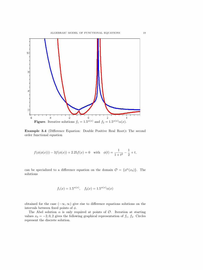
Example 3.4 (Difference Equation: Double Positive Real Root): The secondorder functional equation
f(φ(φ(x)))− 3f(φ(x)) + 2.25f(x) = 0 with φ(t) =1
1 + t2− 1
2+ t,
can be specialized to a difference equation on the domain O = φn(x0). Thesolutions
f1(x) = 1.5α(x), f2(x) = 1.5α(x)α(x)
obtained for the case (−∞,∞) give rise to difference equations solutions on theintervals between fixed points of φ.
The Abel solution α is only required at points of O. Iteration at startingvalues x0 = −2, 0, 2 gives the following graphical representation of f1, f2. Circlesrepresent the discrete solution.
20 JITKA LAITOCHOVÁ
16
7−6
−1
Figure. Iterative solutions y = f(x) for f(φ(φ(x)))− 3f(φ(x)) + 2.25f(x) = 0.
3.4. Conjugate Root Theorem.
Theorem 3. If the characteristic equation
akλk + ak−1λ
k−1 + · · ·+ a1λ+ a0 = 0
has conjugate complex roots
λ1 = λ2 = r(cosω + i sinω),
then the corresponding linear homogeneous functional equation possesses two so-lutions in the form
f1 = rX∗α(x) cos (ωX∗α(x)) ,
f2 = rX∗α(x) sin (ωX∗α(x)) .
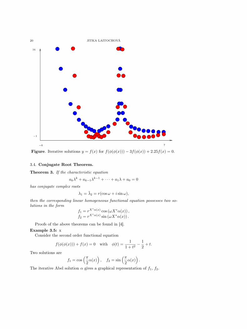
Proofs of the above theorems can be found in [4].Example 3.5: x
Consider the second order functional equation
f(φ(φ(x))) + f(x) = 0 with φ(t) =1
1 + t2− 1
2+ t.
Two solutions are
f1 = cos(π
2α(x)
), f2 = sin
(π2α(x)
).
The iterative Abel solution α gives a graphical representation of f1, f2.
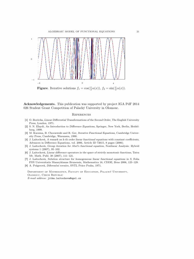
ALGEBRAIC MODEL OF FUNCTIONAL EQUATIONS 21
0 4
−1
0
1
−6
Figure. Iterative solutions f1 = cos(π2α(x)), f2 = sin(π2α(x)).
Acknowledgements. This publication was supported by project IGA PdF 2014026 Student Grant Competition of Palacký University in Olomouc.
References
[1] O. Borùvka, Linear Differential Transformations of the Second Order, The English UniversityPress, London, 1971.
[2] S. N. Elaydi, An Introduction to Difference Equations, Springer, New York, Berlin, Heidel-berg, 1999.
[3] M. Kuczma, B. Choczewski and R. Ger, Iterative Functional Equations, Cambridge Univer-sity Press, Cambridge, Warszawa, 1990.
[4] J. Laitochová, A remark on k-th order linear functional equations with constant coefficients,Advances in Difference Equations, vol. 2006, Article ID 72615, 8 pages (2006).
[5] J. Laitochová, Group iteration for Abel’s functional equation, Nonlinear Analysis: Hybridsystems 1 (2007), 95–102.
[6] J. Laitochová, Linear difference operators in the space of strictly monotonic functions, TatraMt. Math. Publ. 38 (2007), 111–121.
[7] J. Laitochová, Solution structure for homogeneous linear functional equations in S, FoliaFSN Universitatis Masarykianae Brunensis, Mathematica 16, CDDE, Brno 2006, 123–129.
[8] A. Prágerová, Diferenční rovnice, SNTL Práce Praha, 1971.
Department of Mathematics, Faculty of Education, Palacký University,Olomouc, Czech RepublicE-mail address: [email protected]

Matematiqki Bilten ISSN 0351-336XVol.38 (LXIV) No.22014 (23–30) UDC: 517.957:519.85Skopje, Makedonija
BARZILAI-BORWEIN METHOD FORA NONLOCAL ELLIPTIC PROBLEM
MIROSLAV S. PETROV AND TODOR D. TODOROV
Abstract. The object of interest in the present paper is a nonlocal non-linear problem for a general second order elliptic operator. The problemunder consideration represents a model of nonlocal reaction diffusion process.Furthermore, applications in computational biology are also available. Thestrong problem is reduced to a discrete minimization problem. The approxi-mate problem is obtained by Lagrangian finite element discretizations. Dueto its simplicity and efficiency, the Barzilai and Borwein gradient method isused for finding positive solutions with respect to the inhomogeneous strongAllee effect growth pattern. The corresponding fast and stable iterative al-gorithm converges monotonically with respect to the objective functional. Arigorous proof of the monotone convergence theorem is presented. Computerimplementations of the method support the considered theory.
1. Introduction
The population growth is more than eighty millions annually [1]. The humanpopulation increases by 1.2% each year. The global population has grown fromone billion in year 1800 to seven billion in year 2012 [1]. There is a real chanceit reaches more than eleven billion by the end of the century. The exceedingof the resource capacity of an area or environment is called overpopulation. Itaffects directly the growth of the population. The overpopulation problem is veryimportant from economical and social point of view. The mathematical model ofpopulation behavior consists of the nonlinear elliptic problem
∂u
∂t= D∆u+ uf(x, u)
defined on a bounded polygonal domain. The solution u describes the populationdensity, D > 0 denotes the diffusion constant, ∆ is the spatial Laplacian andf(x, u) is the growth rate per capita. If the function f(x, u) is negative when uis small, we call that a strong Allee effect is available [2]. Otherwise if f(x, u) issmaller than the maximum but still positive for small u, we call it a weak Alleeeffect [2]. The application of the reaction-diffusion equation in computational
2010 Mathematics Subject Classification. 65N30, 65K10, 90C06.Key words and phrases. Nonlocal nonlinear problem, Kirchhoff type equation, Barzilai-
Borwein iterative method, finite element approximations.23
24 M. S. PETROV AND T. D. TODOROV
biology is studied by a lot of researchers in the last decades [2]-[5]. A nonlocalreaction-diffusion model
∂u
∂t− a
(∫Ω
|∇u|2)
∆u = f(x, u),
a ∈ C(R+), 0 < m ≤ a(p) ≤Mis studied by M. Chipot, V. Valente, G. V. Caffarelli [6]. More general reaction-diffusion equation is considered by S. A. Sanni [7].
The object of interest in the present paper is the nonlocal nonlinear reaction-diffusion problem investigated by T. D. Todorov [8]. The investigation is carriedout in the case of a general second-order elliptic operator. The nonlocal term in-volved in the strong formulation essentially increases the complexity of the prob-lem and the necessary total computational work. The major contribution of thepresent paper consists of a monotone convergent iterative method for solving thenonlocal nonlinear elliptic problem. A new globalization technique with variablesteplength is obtained. A convergence theorem is proved. The new method iscomputer implemented.
The rest of the article is organized as follows. The problem under considerationis described in Section 2. The weak formulation and discrete problem are obtainedin Section 3. An iterative schemes for solving the nonlocal elliptic problem iscompiled in Section 4. The corresponding algorithm is described briefly step bystep. Section 5 contains some numerical results supporting the considered theory.Concluding remarks are involved in Section 6.
2. Problem definition
Let Ω be a plane polygon. Denote the norm and the seminorm in the realSobolev space Hk(Ω) by ‖·‖k,Ω and the |·|k,Ω. Introduce the norm
||DkF (x)||= sup||ξi||≤11≤i≤k
||DkF (x)(ξ1, ξ2, ..., ξk)||
for the k-th Fréchet derivative DkF (x). The L2-scalar product is denoted by
(u, v) =
∫Ω
uvdx.
Define the spaceV = v ∈ H1(Ω) | v = 0 on Γ.
and the second-order elliptic linear operator
Lu = −2∑
i,j=1
∂
∂xj
(aij
∂u
∂xi
)+ a.u, domL = C2
0
(Ω),
where aij(x) and a(x) belong to C1(Ω), aij = aji, i, j = 1, 2 and a(x) ≥ a0 >0, ∀x ∈ Ω. Assume that L is uniformly elliptic, i.e. there exists a constant α > 0
BARZILAI-BORWEIN METHOD FOR A NONLOCAL ELLIPTIC PROBLEM 25
such that
α
n∑i=1
ξ2i ≤
2∑i,j=1
aij(x)ξiξj , ∀ξ, x ∈ R2. (2.1)
Suppose that:
g ∈ C1(Ω× R),∂g
∂u(x, u) ≥ 0, ∀x ∈ Ω, g(x, 0) = 0, (2.2)
f ∈ L2(Ω) with ||f ||0,Ω 6= 0. (2.3)
Consider the following nonlocal nonlinear elliptic problem
S :
Find u ∈ C20
(Ω)
satisfying :(Lu, u)Lu+ g(x, u) = f(x) in Ω,
u = 0 on ∂Ω.
3. The weak formulation and discretization
Applying Green’s theorem to (S) we obtain the weak formulation
W :
Find u ∈ V such that
a(u, u)a(u, v) + (g(x, u), v) = (f, v) in Ω,
where a(u, v) is the bilinear form
a(u, v) =
∫Ω
2∑i,j=1
aij(x)∂u
∂xi
∂v
∂xjdx+
∫Ω
a(x)uv dx.
and (·, ·) is the L2-scalar product. Since L is a linear continuous and uniformlyV-elliptic operator there exist positive constants α and α such that
α||u||21,Ω ≤ a(u, u), a(u, v) ≤ α||u||1,Ω||v||1,Ω, ∀u, v ∈ V.
Define the objective functional
J(v) =a2(v, v)
4+B(v)− F (v),
where
G(v) =
∫ v
0
g(x, t)dt, F (v) = (f, v) and B(v) =
∫Ω
G(v)dx.
Associate the weak form (W) with the following minimization problem
M : arg minv∈V
J(v).
The existence and uniqueness of the solution of the minimization problem (M)is established in [8, Theorem 1].
Continue with discretization and formulation of the approximate finite elementproblem. Let τh be a regular family of conforming finite element triangulationsobtained by Lagrangian finite elements of degree n, Vh ⊂ V be the correspondingfinite element space, Nh = aimi=1 be the set of all interior nodes of τh and
26 M. S. PETROV AND T. D. TODOROV
ϕi(x)mi=1 be the nodal bases functions of Vh. Consider the following discreteproblem
Wh :
Find a function uh ∈ Vh satisfying
a(uh, uh)a(uh, vh) + (g(x, uh), vh) = (f, vh), ∀vh ∈ Vh.
The finite element solution can be presented in the form
uh(x) = U · Φ(x) =
m∑i=1
Uiϕi(x) ∈ Vh,
where Ui = uh(ai). As in [8] we interpolate the function g by a Vh interpolant
Ihg =
m∑i=1
g(ai, u(ai))ϕi.
Compile the quartic problem
Qh :
Find a function uh ∈ Vh that satisfiesa(uh, uh)a(uh, vh) + (gh, vh) = (f, vh), ∀vh ∈ Vh
,
where gh = Ihg. Define
Gh(v) =
∫ v
0
gh(x, t)dt, Bh(v) =
∫Ω
Gh(v)dx
and corresponding objective functionals:
J(vh) =1
4a2(vh, vh) +B(vh)− F (vh), vh ∈ Vh,
Jh(vh) =1
4a2(vh, vh) +Bh(vh)− F (vh), vh ∈ Vh
for the problems (Wh) and (Qh).Remark that
DJh(uh)vh = a(uh, uh)a(uh, vh) + (gh, vh)− (f, vh), ∀vh ∈ Vh.
4. A globalization technique with variable steplength for solvingthe discrete problem
Consider the following unconstraint minimization problem
Mh : arg minv∈Vh
J(v).
Define the Barzilai-Borwein gradient method
(uk+1, v) = (uk, v)− 1
αkDJ(uk)v, k ≥ 1 (4.1)
with the steplength
αk =(a(uk, uk) + a(uk−1, uk−1)) a(sk−1, sk−1) + ((g(x, uk) + g(x, uk−1))sk−1, sk−1)
2||sk−1||21,Ω,
(4.2)sk−1 = uk − uk−1
BARZILAI-BORWEIN METHOD FOR A NONLOCAL ELLIPTIC PROBLEM 27
obtained by T. D. Todorov [8]. He proved that the steplength (4.2) produces muchbetter results in the quartic case than the classical steplength
βk =DF (uk)sk−1
||sk−1||21,Ω(4.3)
analyzed by E. G. Birgin, J. M. Martínez and M. Raydan [9]. In the proof of [8,Theorem 2] was established that
0 < α∗ < αk < α∗, ∀k ∈ N, (4.4)
where α∗ and α∗ are positive constants. The validity of (4.4) depends on thedistance between the initial guesses and the weak solution. If the initial guessesare faraway from the weak solution αk could become negative for some k. Thatis why in such cases we cannot guarantee monotone convergence of the objectivefunctional. Moreover the lack of estimate (4.4) can lead to divergence of the twopoint step size gradient method (4.1-4.2).
In this section we propose a monotone convergent algorithm for the two pointgradient method in the quartic case.
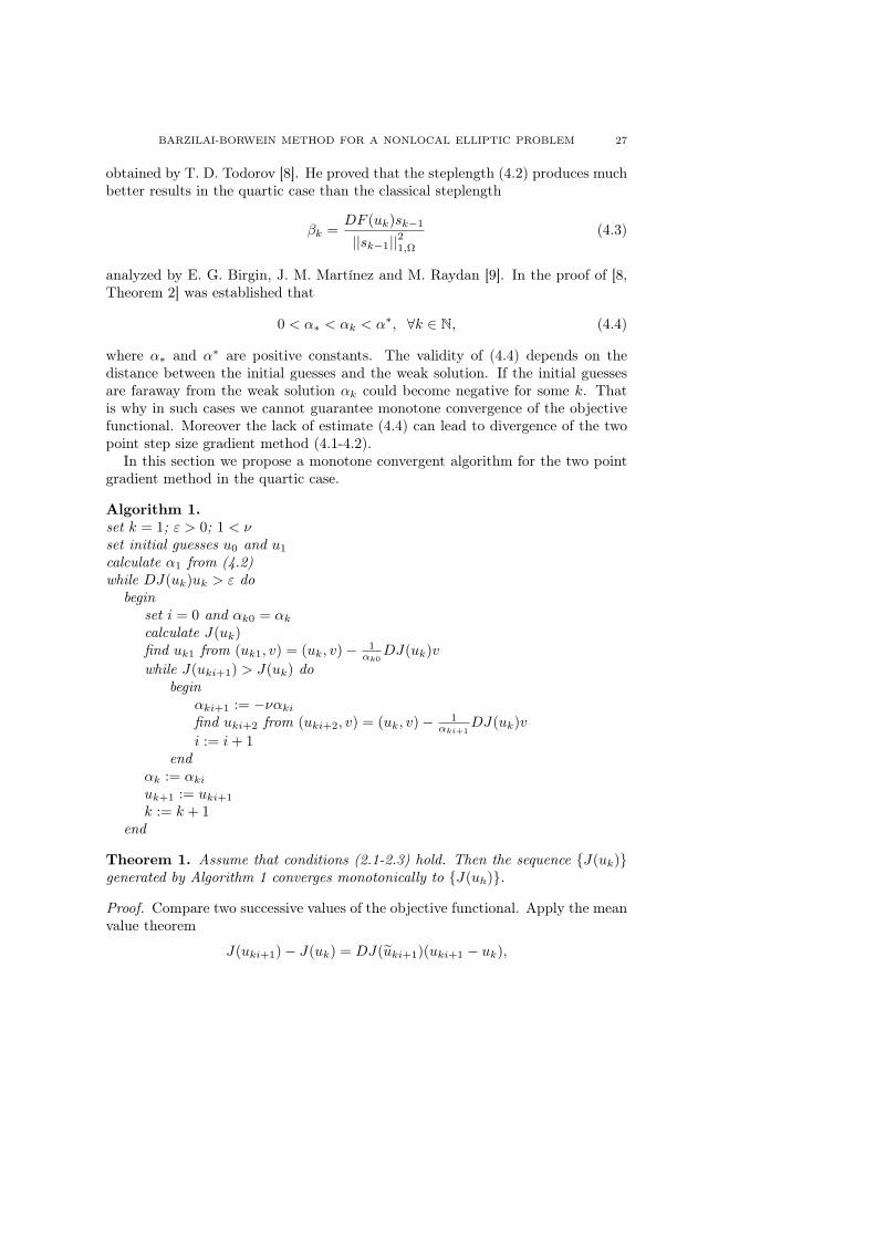
Algorithm 1.set k = 1; ε > 0; 1 < νset initial guesses u0 and u1
calculate α1 from (4.2)while DJ(uk)uk > ε do
beginset i = 0 and αk0 = αkcalculate J(uk)find uk1 from (uk1, v) = (uk, v)− 1
αk0DJ(uk)v
while J(uki+1) > J(uk) dobegin
αki+1 := −ναkifind uki+2 from (uki+2, v) = (uk, v)− 1
αki+1DJ(uk)v
i := i+ 1end
αk := αkiuk+1 := uki+1
k := k + 1end
Theorem 1. Assume that conditions (2.1-2.3) hold. Then the sequence J(uk)generated by Algorithm 1 converges monotonically to J(uh).
Proof. Compare two successive values of the objective functional. Apply the meanvalue theorem
J(uki+1)− J(uk) = DJ(uki+1)(uki+1 − uk),
28 M. S. PETROV AND T. D. TODOROV
where uki+1 = uk + ϑ(uki+1 − uk), ϑ ∈ (0, 1). From the definition of uki+1 wehave
J(uki+1)− J(uk) = − 1
αkiDJ(uki+1)DJ(uk).
Remember that the functional J(u) is twice Fréchet differentiable. Therefore, fromthe sign preservation property, there is a neighborhood
Uε(uk) = v ∈ Vh | ‖uk − v‖1,Ω < ε
such that DJ(v)DJ(uk) > 0 ∀v ∈ Uε(uk). We haveuki uki→ +∞
since|αki|→ +∞i→ +∞ . Then there is an integer i0 such that
uki+1 ∈ Uε(uk) ∀i ≥ i0. (4.5)
Let i be the smallest i satisfying (4.5) and αki > 0. Then
J(uki+1)− J(uk) = − 1
αkiDJ(uki)DJ(uk) < 0.
We choose uk+1 = uki+1 and obtain J(uk+1) < J(uk). Thus we proved that thesequence J(uk) is monotone decreasing. Since J(uk) ≥ J(uh) [8] we concludethat J(uk) converges monotonically.
It remains to prove that
limk→+∞
J(uk) = J(uh). (4.6)
Suppose the negation of (4.6) namelyuk u∞k → +∞ and ‖u∞ − uh‖1,Ωh 6= 0. Then
J(u∞) = infk∈N
J(uk). (4.7)
Choosing a sufficiently large α∞ > 0 we obtain
u∗ = u∞ −1
α∞DJ(u∞)
and J(u∗) < J(u∞). The last result contradicts to (4.7). Therefore (4.6) is validwhich completes the proof.
5. Numerical Tests
Consider an initial uniform triangulation of the unit square Ω by 18 cubictriangular Lagrangian finite elements. Obtain triangulations with 162 and 1458applying the Jung and Todorov [10] refinement strategy. All numerical tests areexecuted by Andreev and Todorov [11] cubature formula of degree five. Thiscubature formula is appropriate for obtaining optimal convergence properties withrespect to the cubic Lagrangian finite element.
Denote the error functional by
E(v) = |DJh(v)v|and ε = 10−6.
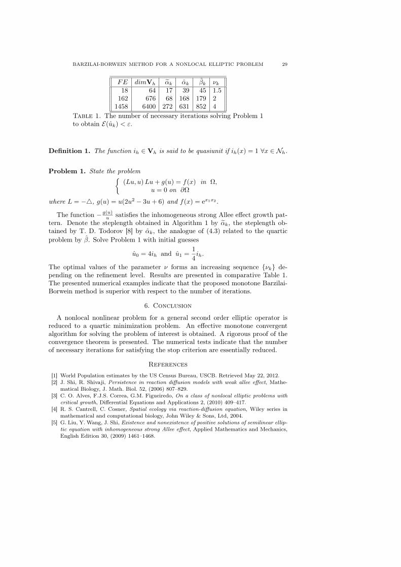
BARZILAI-BORWEIN METHOD FOR A NONLOCAL ELLIPTIC PROBLEM 29
FE dimVh αk αk βk νk18 64 17 39 45 1.5
162 676 68 168 179 21458 6400 272 631 852 4
Table 1. The number of necessary iterations solving Problem 1to obtain E(uk) < ε.
Definition 1. The function ih ∈ Vh is said to be quasiunit if ih(x) = 1 ∀x ∈ Nh.
Problem 1. State the problem(Lu, u)Lu+ g(u) = f(x) in Ω,
u = 0 on ∂Ω
where L = −4, g(u) = u(2u2 − 3u+ 6) and f(x) = ex1x2 .
The function − g(u)u satisfies the inhomogeneous strong Allee effect growth pat-
tern. Denote the steplength obtained in Algorithm 1 by αk, the steplength ob-tained by T. D. Todorov [8] by αk, the analogue of (4.3) related to the quarticproblem by β. Solve Problem 1 with initial guesses
u0 = 4ih and u1 =1
4ih.
The optimal values of the parameter ν forms an increasing sequence νk de-pending on the refinement level. Results are presented in comparative Table 1.The presented numerical examples indicate that the proposed monotone Barzilai-Borwein method is superior with respect to the number of iterations.
6. Conclusion
A nonlocal nonlinear problem for a general second order elliptic operator isreduced to a quartic minimization problem. An effective monotone convergentalgorithm for solving the problem of interest is obtained. A rigorous proof of theconvergence theorem is presented. The numerical tests indicate that the numberof necessary iterations for satisfying the stop criterion are essentially reduced.
References
[1] World Population estimates by the US Census Bureau, USCB. Retrieved May 22, 2012.[2] J. Shi, R. Shivaji, Persistence in reaction diffusion models with weak allee effect, Mathe-
matical Biology, J. Math. Biol. 52, (2006) 807–829.[3] C. O. Alves, F.J.S. Correa, G.M. Figueiredo, On a class of nonlocal elliptic problems with
critical growth, Differential Equations and Applications 2, (2010) 409–417.[4] R. S. Cantrell, C. Cosner, Spatial ecology via reaction-diffusion equation, Wiley series in
mathematical and computational biology, John Wiley & Sons, Ltd, 2004.[5] G. Liu, Y. Wang, J. Shi, Existence and nonexistence of positive solutions of semilinear ellip-
tic equation with inhomogeneous strong Allee effect, Applied Mathematics and Mechanics,English Edition 30, (2009) 1461–1468.
30 M. S. PETROV AND T. D. TODOROV
[6] M. Chipot, V. Valente, G.V. Caffarelli, Remarks on a nonlocal problem involving the Dirich-let energy, Rendiconti del Seminario Matematico della universitaÂădi Padova 110, (2003)199–220.
[7] S. A. Sanni, Nonlocal degenerate reaction-diffusion equations with general nonlinear diffu-sion term, Electronic Journal of Differential Equations, vol. 2014, 124 (2014), 1–27.
[8] T. D. Todorov, A nonlocal problem for a general second-order elliptic operator, Computers& Mathematics with Applications, vol.69, issue 5, (2015), 411-422.
[9] E. G. Birgin, J. M. Martínez, M. Raydan, Spectral Projected Gradient methods: Review andPerspectives, Journal of Statistical Software, vol. 60, 3, 2014.
[10] M. Jung and T. D. Todorov, Isoparametric multigrid method for reaction-diffusion equa-tions, Applied Numerical Mathematics, 56, (2006) 1570–1583.
[11] A. B. Andreev, T. D. Todorov, Isoparametric numerical integration on triangular finiteelement meshes, Comptes rendus de l’Academie bulgare des Sciences, 17, vol. 57, (2004)37–44.
Department of Technical Mechanics, Technical University,5300 Gabrovo, BulgariaE-mail address: [email protected]
Department of Mathematics, Technical University,5300 Gabrovo, BulgariaE-mail address: [email protected]
Matematiqki Bilten ISSN 0351-336XVol.38 (LXIV) No.22014 (31–51) UDC: 517.417.12:517.518.28Skopje, Makedonija
GENERALIZATIONS OF STEFFENSEN’S INEQUALITYVIA n WEIGHT FUNCTIONS
A. AGLIĆ ALJINOVIĆ, J. PEČARIĆ, AND A. PERUŠIĆ PRIBANIĆ
Abstract. New generalizations of Steffensen’s inequality are obtained bymeans of weighted Montgomery identity with n different weight functions.Instead for a nondecreasing (1-convex) function our generalization hold for an-convex function. Further, functionals associated to these new generaliza-tions are observed and used to generate n−exponentially and exponentiallyconvex functions as well as to obtain new Stolarsky type means related tothese functionals.
1. Introduction
The well-known Steffensen’s inequality states (see [15])
Theorem 1. Let f, g : [a, b] → R be integrable mappings on [a, b] such that f isnonincreasing and 0 ≤ g (t) ≤ 1 for t ∈ [a, b]. Then∫ b
b−λf (t) dt ≤
∫ b
a
f (t) g (t) dt ≤∫ a+λ
a
f (t) dt (1.1)
where λ =∫ bag (t) dt.
J. F. Steffensen proved this inequality in 1918 and since then it was generalizedin numerous ways. Extensive overview of these generalizations can be found in[10] or [14].
In the recent paper [3] the next weighted Euler identity is obtained:
Theorem 2. Let f : [a, b]→ R be n-times differentiable on [a, b] , n ∈ N with f (n): [a, b] → R integrable on [a, b]. Let wi : [a, b] → [0,∞〉, i = 1, .., n be a sequenceof n integrable functions satisfying
∫ bawi (t) dt = 1 and Wi (t) =
∫ tawi (x) dx for
2010 Mathematics Subject Classification. Primary: 26D15, 26A48 .Key words and phrases. Steffensen’s inequality, Montgomery identity, n-exponentially convex
function.31
32 A. AGLIĆ ALJINOVIĆ, J. PEČARIĆ, AND A. PERUŠIĆ PRIBANIĆ
t ∈ [a, b], Wi (t) = 0 for t < a and Wi (t) = 1 for t > b, for all i = 1, .., n. For anyx ∈ [a, b] define weighted Peano kernel:
Pwi (x, t) =
Wi (t) , a ≤ t ≤ x,
Wi (t)− 1 x < t ≤ b.Then it holds
f (x)−∫ b
a
w1 (t) f (t) dt−n−2∑k=0
(∫ b
a
wk+2 (t) f (k+1) (t) dt
)
·
(∫ b
a
· · ·∫ b
a
Pw1(x, t1)
k∏i=1
Pwi+1(ti, ti+1) dt1 · · · dtk+1
)
=
∫ b
a
· · ·∫ b
a
Pw1(x, t1)
n−1∏i=1
Pwi+1(ti, ti+1) f (n) (tn) dt1 · · · dtn. (1.2)
If we take wi ≡ w, i = 1, .., n identity (1.2) reduces to identity obtained in[1], and for n = 1, it reduces to the weighted Montgomery identity given byPečarić in [11]
f (x)−∫ b
a
w1 (t) f (t) dt =
∫ b
a
Pw1(x, t1) f
′(t1) dt1.
The aim of this paper is to generalize Steffensen’s inequality by using theweighted Euler identity (1.2). In a such way new generalizations Steffensen’sinequality for a n-convex function are obtained in Section 2 and Section 3. Incase n = 1 Steffensen’s inequality (1.1) is recaptured since 1-convex functions aremonotonic (nondecreasing) functions. In such way we generalize for any n ∈ Nresults obtained in [6] for n = 1. In Section 4 estimates of the difference of theleft-hand and right-hand sides of the obtained inequalities are given. In Section 5,three functionals associated to these new generalizations are considered and usedto generate n−exponentially and exponentially convex functions. In Section 6,new Stolarsky type means related to these functionals are obtained.
2. The difference between two weighted integral means
Next, we subtract two generalized weighted Montgomery identities (1.2) to ob-tain identity for the difference between two weighted integral means, each havingits own weight, on two different intersecting intervals [a, b] and [c, d]. This identityis given in the next theorem for both possible cases, when one interval is a subsetof the other [c, d] ⊆ [a, b] and for overlapping intervals [a, b] ∩ [c, d] = [c, b]. Theother two possible cases, when [a, b] ∩ [c, d] 6= ∅ we simply get by replacementa↔ c, b↔ d. For that purpose we denote
T [a,b]w1,..,wn (x) =
n−2∑k=0
(1∫ b
awk+2 (t) dt
∫ b
a
wk+2 (t) f (k+1) (t) dt
)
GENERALIZATIONS OF STEFFENSEN’S INEQUALITY 33
·
(∫ b
a
· · ·∫ b
a
Pw1 (x, t1)
k∏i=1
Pwi+1 (ti, ti+1) dt1 · · · dtk+1
).
Theorem 3. Let f : [a, b]∪[c, d]→ R be n-times differentiable on [a, b]∪[c, d] , n ∈N with f (n) : [a, b] ∪ [c, d]→ R integrable on [a, b] ∪ [c, d]. Let wi : [a, b]→ [0,∞〉,i = 1, .., n be a sequence of n integrable functions, Wi (t) =
∫ tawi (x) dx for t ∈
[a, b], Wi (t) = 0 for t < a and Wi (t) =∫ bawi (x) dx for t > b, for all i = 1, .., n.
Also, let ui : [c, d] → [0,∞〉, i = 1, .., n be a sequence of n integrable functionsUi (t) =
∫ tcui (x) dx for t ∈ [c, d], Ui (t) = 0 for t < c and Ui (t) =
∫ dcui (x) dx for
t > d, for all i = 1, .., n. For any x ∈ [a, b] ∪ [c, d] define weighted Peano kernel:
Pwi(x, t)=
1
Wi(b)Wi (t) , a ≤ t ≤ x,
1Wi(b)
Wi (t)− 1, x < t ≤ b,0, t /∈ [a, b] ,
Pui(x, t) =
1
Ui(d)Ui (t) , c ≤ t ≤ x,
1Ui(d)
Ui (t)− 1, x < t ≤ d,0, t /∈ [c, d] .
Then if Wi (b) 6= 0 and Ui (d) 6= 0 for i = 1, .., n, for any x ∈ [a, b] ∩ [c, d] itholds
1∫ dcu1(t)dt
∫ dcu1 (t) f (t) dt− 1∫ b
aw1(t)dt
∫ baw1 (t) f (t) dt−−T [a,b]
w1,..,wn(x) + T[c,d]u1,..,un(x) =
=∫maxb,dmina,c K (x, t1, . . . , tn) f (n) (tn) dtn
(2.1)where
K (x, t1, . . . , tn) =
∫ maxb,d
mina,c· · ·∫ maxb,d
mina,c
[Pw1
(x, t1)
n−1∏i=1
Pwi+1(ti, ti+1) (2.2)
−Pu1(x, t1)
n−1∏i=1
Pui+1(ti, ti+1)
]dt1 · · · dtn−1
Proof. We apply (1.2) with x ∈ [a, b] ∩ [c, d] and n normalized weight functionswi (t) /Wi (b), t ∈ [a, b], i = 1, .., n and then once again with n normalized weightfunctions ui (t) /Ui (d), t ∈ [c, d], i = 1, .., n. By subtracting these two identitieswe obtain
1∫ dcu1 (t) dt
∫ d
c
u1 (t) f (t) dt− 1∫ baw1 (t) dt
∫ b
a
w1 (t) f (t) dt− T [a,b]w1,..,wn(x) + T [c,d]
u1,..,un(x)
=
∫ b
a
· · ·∫ b
a
Pw1(x, t1)
n−1∏i=1
Pwi+1(ti, ti+1) f (n) (tn) dt1 · · · dtn
−∫ d
c
· · ·∫ d
c
Pu1(x, t1)
n−1∏i=1
Pui+1(ti, ti+1) f (n) (tn) dt1 · · · dtn
34 A. AGLIĆ ALJINOVIĆ, J. PEČARIĆ, AND A. PERUŠIĆ PRIBANIĆ
=
∫ maxb,d
mina,cK (x, t1, . . . , tn) f (n) (tn) dtn
and (2.1) is proved.
Consider the sequence (Bk (t) , k ≥ 0) of Bernoulli polynomials which is uniquelydetermined by the following identities:
B′k (t) = kBk−1 (t) , k ≥ 1, B0 (t) = 1
andBk (t+ 1)−Bk (t) = ktk−1, k ≥ 0.
The values Bk = Bk (0), k ≥ 0 are known as Bernoulli numbers. For our purposes,the first five Bernoulli polynomials are
B0 (t) = 1, B1 (t) = t− 1
2, B2 (t) = t2 − t+
1
6,
B3 (t) = t3 − 3
2t2 +
1
2t, B4 (t) = t4 − 2t3 + t2 − 1
30.
Let (B∗k (t) , k ≥ 0) be a sequence of periodic functions of period 1, related toBernoulli polynomials as
B∗k (t) = Bk (t) , 0 ≤ t < 1, B∗k (t+ 1) = B∗k (t) , t ∈ R.
From the properties of Bernoulli polynomials it easily follows that B∗0 (t) = 1, B∗1is discontinuous function with a jump of −1 at each integer, while B∗k , k ≥ 2, arecontinuous functions.
Corollary 3.1. Let f : [a, b] ∪ [c, d] → R be n-times differentiable on [a, b] ∪[c, d] , n ∈ N with f (n) : [a, b]∪ [c, d]→ R integrable on [a, b]∪ [c, d]. Let w : [a, b]→[0,∞〉 and u : [c, d]→ [0,∞〉 be integrable weight functions, W (t) =
∫ taw (x) dx for
t ∈ [a, b], W (t) = 0 for t < a and W (t) =∫ baw (x) dx for t > b, U (t) =
∫ tcu (x) dx
for t ∈ [c, d], U (t) = 0 for t < c and U (t) =∫ dcu (x) dx for t > d. Then if
W (b) 6= 0 and U (d) 6= 0, for any x ∈ [a, b] ∩ [c, d] it holds
1∫ dcu (t) dt
∫ d
c
u (t) f (t) dt− 1∫ baw (t) dt
∫ b
a
w (t) f (t) dt− T [a,b]w (x) + T [c,d]
u (x)
=(b− a)
n−2
(n− 1) !
∫ b
a
(∫ b
a
Pw (x, s)
[Bn−1
(s− ab− a
)−B∗n−1
(s− tb− a
)]ds
)f (n) (t) dt
− (d− c)n−2
(n− 1) !
∫ d
c
(∫ d
c
Pu (x, s)
[Bn−1
(s− cd− c
)−B∗n−1
(s− td− c
)]ds
)f (n) (t) dt
(2.3)
where
T [a,b]w (x) =
n−2∑k=0
(b− a)k−1
k!
(∫ b
a
Pw (x, t)Bk
(t− ab− a
)dt
)(f (k) (b)− f (k) (a)
)
GENERALIZATIONS OF STEFFENSEN’S INEQUALITY 35
T [c,d]u (x) =
n−2∑k=0
(d− c)k−1
k!
(∫ d
c
Pw (x, t)Bk
(t− cd− c
)dt
)(f (k) (d)− f (k) (c)
)Proof. We apply identity (2.1) with w1 ≡ w, wi ≡ 1
b−a , i = 2, .., n and u1 ≡ u,ui ≡ 1
d−c , i = 2, .., n. Then Pwi (x, t) and Pui (x, t) for i = 2, .., n reduce to
Pa,b (x, t) =
t−ab−a , a ≤ t ≤ x,t−bb−a , x < t ≤ b,0, t /∈ [a, b] .
and Pc,d (x, t) =
t−cd−c , c ≤ t ≤ x,t−dd−c , x < t ≤ d,0, t /∈ [c, d] .
Since the the next two identities hold (see [4])∫ b
a
· · ·∫ b
a
Pa,b(x, s1)
(k−1∏i=1
Pa,b(si, si+1)
)ds1 · · · dsk =
(b− a)k
k!Bk
(x− ab− a
)and ∫ b
a
· · ·∫ b
a
Pa,b (x, s1)
(n−2∏i=1
Pa,b (si, si+1)
)ds1 · · · dsn−2
=(b− a)
n−2
(n− 1) !
[Bn−1
(x− ab− a
)−B∗n−1
(x− snb− a
)]it follows that
1
b− a
∫ b
a
· · ·∫ b
a
Pw (x, t1)
k∏i=1
Pa,b (ti, ti+1) dt1 · · · dtk+1
=(b− a)
k−1
k!
(∫ b
a
Pw (x, t)Bk
(t− ab− a
)dt
)and∫ b
a
· · ·∫ b
a
Pw (x, t1)
n−1∏i=1
Pa,b (ti, ti+1) f (n) (tn) dt1 · · · dtn
=(b− a)
n−2
(n− 1) !
∫ b
a
(∫ b
a
Pw (x, s)
[Bn−1
(s− ab− a
)−B∗n−1
(s− tb− a
)]ds
)f (n) (t) dt.
Consequently T [a,b]w1,..,wn (x) reduces to
T[a,b]w (x)
= 1b−a
∑n−2k=0
(∫ ba· · ·∫ baPw (x, t1)
k∏i=1
Pa,b (ti, ti+1) dt1 · · · dtk+1
)(f (k) (b)− f (k) (a)
)=∑n−2k=0
(b−a)k−1
k!
(∫ baPw (x, t)Bk
(t−ab−a
)dt) (f (k) (b)− f (k) (a)
)and similarly T [c,d]
u1,..,un (x) to T [c,d]u (x). Finally∫ maxb,d
mina,cK (x, t1, . . . , tn) f (n) (tn) dtn
36 A. AGLIĆ ALJINOVIĆ, J. PEČARIĆ, AND A. PERUŠIĆ PRIBANIĆ
=(b− a)
n−2
(n− 1) !
∫ b
a
(∫ b
a
Pw (x, s)
[Bn−1
(s− ab− a
)−B∗n−1
(s− tb− a
)]ds
)f (n) (t) dt
− (d− c)n−2
(n− 1) !
∫ d
c
(∫ d
c
Pu (x, s)
[Bn−1
(s− cd− c
)−B∗n−1
(s− td− c
)]ds
)f (n) (t) dt
and identity (2.1) reduces to identity (2.3).
Corollary 3.2. Let f : [a, b] ∪ [c, d] → R be n-times differentiable on [a, b] ∪[c, d] , n ∈ N with f (n) : [a, b]∪ [c, d]→ R integrable on [a, b]∪ [c, d]. Let w : [a, b]→[0,∞〉 and u : [c, d]→ [0,∞〉 be integrable weight functions, W (t) =
∫ taw (x) dx for
t ∈ [a, b], W (t) = 0 for t < a and W (t) =∫ baw (x) dx for t > b, U (t) =
∫ tcu (x) dx
for t ∈ [c, d], U (t) = 0 for t < c and U (t) =∫ dcu (x) dx for t > d. Then if
W (b) 6= 0 and U (d) 6= 0, for any x ∈ [a, b] ∩ [c, d] it holds
1∫ dcu (t) dt
∫ d
c
u (t) f (t) dt− 1∫ baw (t) dt
∫ b
a
w (t) f (t) dt− T [a,b]w,n (x) + T [c,d]
u,n (x)
=
∫ maxb,d
mina,cK (x, t1, . . . , tn) f (n) (tn) dtn (2.4)
where
T [a,b]w,n (x) =
n−2∑k=0
(1∫ b
aw (t) dt
∫ b
a
w (t) f (k+1) (t) dt
)
·
(∫ b
a
· · ·∫ b
a
Pw (x, t1)
k∏i=1
Pw (ti, ti+1) dt1 · · · dtk+1
),
T [c,d]u,n (x) =
n−2∑k=0
(1∫ d
cu (t) dt
∫ d
c
u (t) f (k+1) (t) dt
)
·
(∫ d
c
· · ·∫ d
c
Pu (x, t1)
k∏i=1
Pu (ti, ti+1) dt1 · · · dtk+1
),
and
K (x, t1, . . . , tn) =
∫ maxb,d
mina,c· · ·∫ maxb,d
mina,c
[Pw (x, t1)
n−1∏i=1
Pw (ti, ti+1)
= −Pu (x, t1)
n−1∏i=1
Pu (ti, ti+1)
]dt1 · · · dtn−1
Proof. We apply identity (2.1) with wi ≡ w, i = 1, .., n. Then T[a,b]w1,..,wn (x),
T[c,d]u1,..,un (x) and K (x, t1, . . . , tn) reduce to T [a,b]
w,n (x), T [c,d]u,n (x) and K (x, t1, . . . , tn)
respectively.
GENERALIZATIONS OF STEFFENSEN’S INEQUALITY 37
Remark 2.1: Identity (2.3) was previously obtained in [2]. In a special case foruniform normalized weight function w, for the case [c, d] ⊆ [a, b] it was obtainedin [12] and for the case [a, b] ∩ [c, d] = [c, b] in [5]. Identity (2.4), in a special casefor uniform normalized weight function w, for c = d as a limit case and n = 2 wasobtained in [1], while for n = 3 it was obtained in [4].
Theorem 4. Let f : [a, b] ∪ [c, d] → R be n-convex function on [a, b] ∪ [c, d] , n ∈N. Let wi : [a, b] → [0,∞〉, i = 1, .., n be a sequence of n integrable functions,Wi (t) =
∫ tawi (x) dx for t ∈ [a, b], Wi (t) = 0 for t < a and Wi (t) =
∫ bawi (x) dx
for t > b,for all i = 1, .., n. Also, let ui : [c, d] → [0,∞〉, i = 1, .., n be a sequenceof n integrable functions, Ui (t) =
∫ tcui (x) dx for t ∈ [c, d], Ui (t) = 0 for t < c
and Ui (t) =∫ dcui (x) dx for t > d, for all i = 1, .., n. If
K ≥ 0 (2.5)
where K is the function defined by (2.2), then for any x ∈ [a, b] ∩ [c, d] it holds
1∫ baw1 (t) dt
∫ b
a
w1 (t) f (t) dt+T [a,b]w1,..,wn(x) ≤ 1∫ d
cu1 (t) dt
∫ d
c
u1 (t) f (t) dt+T [c,d]u1,..,un(x) .
(2.6)
Proof. Since f is a n-convex function, without loss of generality we can assume (see[14, p. 293]) that f (n) exists and is continuous. By using the (2.1) and f (n) ≥ 0the proof follows.
Remark 2.2: Inequality (2.6) holds also if f is n-concave and K ≤ 0. If f isn-concave and K ≥ 0 or f is n-convex and K ≤ 0 the inequality (2.6) is reversed.
3. Generalizations of Steffensen’s inequality
Corollary 4.1. Let f : [a, b] ∪ [a, a+ λ] → R be n-convex function on [a, b] ∪[a, a+ λ] , n ∈ N. Let wi : [a, b] → [0,∞〉, i = 1, .., n and ui : [a, a+ λ] → [0,∞〉,i = 1, .., n be two sequences of weight functions as in Theorem 3. If
K ≥ 0 (3.1)
where K is the function defined by (2.2), then for any x ∈ [a, b]∩ [a, a+ λ] it holds:1∫ b
aw1(t)dt
∫ baw1 (t) f (t) dt+ T
[a,b]w1,..,wn(x) ≤
≤ 1∫ a+λa
u1(t)dt
∫ a+λau1 (t) f (t) dt+ T
[a,a+λ]u1,..,un(x) .
(3.2)
In case f is n-concave function inequality (3.2) holds if K ≤ 0.
Proof. We apply Theorem 4 with [c, d] = [a, a+ λ].
Remark 3.1: For every differentiable, nonincreasing function f : [a, b]∪[a, a+ λ]→R and w : [a, b] → [0,∞〉 and u : [a, a+ λ] → [0,∞〉 some weight functions suchthat
∫ baw (t) dt =
∫ a+λa
u (t) dt inequality (3.2) for n = 1 reduces to∫ b
a
w (t) f (t) dt ≤∫ a+λ
a
u (t) f (t) dt

38 A. AGLIĆ ALJINOVIĆ, J. PEČARIĆ, AND A. PERUŠIĆ PRIBANIĆ
while condition K ≤ 0 reduces to∫ x
a
u (t) dt ≥∫ x
a
w (t) dt for x ∈ [a, a+ λ] and∫ b
x
w (t) dt ≥ 0 for x ∈ 〈a+ λ, b] ,
(3.3)in case 0 < λ ≤ b− a and to∫ x
a
u (t) dt ≥∫ x
a
w (t) dt for x ∈ [a, b] and∫ a+λ
x
u (t) dt ≤ 0 for x ∈ 〈b, a+ λ] ,
in case λ > b− a.Further for u ≡ 1 we have
∫ baw (t) dt =
∫ a+λa
u (t) dt = λ. Thus if 0 ≤ w (t) ≤ 1for t ∈ [a, b] then λ ≤ b− a and it’s easy to see that (3.3) is fulfilled. In a such away the right-hand side of the Steffensen’s inequality (1.1) is recaptured.
Corollary 4.2. Let f : [a, b] ∪ [b− λ, b] → R be n-convex function on [a, b] ∪[b− λ, b] , n ∈ N. Let wi : [a, b] → [0,∞〉, i = 1, .., n and ui : [b− λ, b] → [0,∞〉,i = 1, .., n be two sequences of weight functions as in Theorem 3. If
K ≤ 0 (3.4)
where K is the function defined by (2.2), then for any x ∈ [a, b]∩ [b− λ, b] it holds:1∫ b
aw1(t)dt
∫ baw1 (t) f (t) dt+ T
[a,b]w1,..,wn(x) ≥
≥ 1∫ bb−λ u1(t)dt
∫ bb−λu1 (t) f (t) dt+ T
[b−λ,b]u1,..,un(x)
(3.5)
In case f is n-concave function inequality (3.5) holds if K ≥ 0.
Proof. We apply Theorem 4 with [c, d] = [b− λ, b].
Remark 3.2: For every differentiable, nonincreasing function f : [a, b]∪[b− λ, b]→R and w : [a, b] → [0,∞〉 and u : [b− λ, b] → [0,∞〉 some weight functions suchthat
∫ baw (t) dt =
∫ bb−λ u (t) dt inequality (3.5) for n = 1 reduces to∫ b
a
w (t) f (t) dt ≥∫ b
b−λu (t) f (t) dt
while condition K ≥ 0 reduces to∫ x
a
w (t) dt ≥ 0 for x ∈ [a, b− λ] and∫ x
b−λu (t) dt ≤
∫ x
a
w (t) dt for x ∈ 〈b− λ, b]
(3.6)in case 0 < λ ≤ b− a and to∫ x
b−λu (t) dt ≤ 0 for x ∈ [b− λ, a] and
∫ x
b−λu (t) dt ≤
∫ x
a
w (t) dt for x ∈ 〈a, b] ,
in case λ > b− a.Further for u ≡ 1 we have
∫ baw (t) dt =
∫ bb−λ u (t) dt = λ. Thus if 0 ≤ w (t) ≤ 1
for t ∈ [a, b] then λ ≤ b− a and it’s easy to see that (3.6) is fulfilled since
x− b+ λ =
∫ x
b−λu (t) dt ≤
∫ x
a
w (t) dt = λ−∫ b
x
w (t) dt.
GENERALIZATIONS OF STEFFENSEN’S INEQUALITY 39
In a such a way the left-hand side of the Steffensen’s inequality (1.1) is recaptured.
4. Lp inequalities
Here, the symbol Lp[a,b] (1 ≤ p <∞) denotes the space of p-power integrablefunctions on the interval [a, b] equipped with the norm
‖f‖p,[a,b] =
(∫ b
a
|f (t)|p dt
) 1p
and L∞[a,b]denotes the space of essentially bounded functions on [a, b] with the norm
‖f‖∞,[a,b] = ess supt∈[a,b]
|f (t)| .
Theorem 5. Suppose that all the assumptions of Theorem 3 hold. Additionallyassume (p, q) is a pair of conjugate exponents, that is 1 ≤ p, q ≤ ∞, 1
p + 1q = 1,
and f (n) ∈ Lp[a,b]∪[c,d]. Then the following inequality holds∣∣∣∣∣ 1∫ dcu1 (t) dt
∫ d
c
u1 (t) f (t) dt− T [a,b]w1,..,wn (x)
− 1∫ baw1 (t) dt
∫ b
a
w1 (t) f (t) dt+ T [c,d]u1,..,un (x)
∣∣∣∣∣≤ ‖K (x, t1, . . . , tn−1, ·)‖q,[mina,c,maxb,d]
∥∥∥f (n)∥∥∥p,[mina,c,maxb,d]
(4.1)
Inequality (4.1) is sharp for 1 < p ≤ ∞ and for p = 1 constant‖K (x, t1, . . . , tn−1, ·)‖q,[mina,c,maxb,d] is the best possible.
Proof. By taking the modulus on (2.1) and applying the Hölder inequality weobtain ∣∣∣∣∣ 1∫ d
cu1 (t) dt
∫ d
c
u1 (t) f (t) dt− T [a,b]w1,..,wn (x)
− 1∫ baw1 (t) dt
∫ b
a
w1 (t) f (t) dt+ T [c,d]u1,..,un (x)
∣∣∣∣∣=
∣∣∣∣∣∫ maxb,d
mina,cK (x, t1, . . . , tn) f (n) (tn) dtn
∣∣∣∣∣≤ ‖K (x, t1, . . . , tn−1, ·)‖q,[mina,c,maxb,d]
∥∥∥f (n)∥∥∥p,[mina,c,maxb,d]
Let’s denote C (t) = K (x, t1, . . . , tn−1, t). For the proof of the sharpness we willfind a function f for which the equality in (4.1) is obtained.
For 1 < p <∞ take f to be such that
f (n) (t) = sgn C (t) · |C (t)|1p−1 .
40 A. AGLIĆ ALJINOVIĆ, J. PEČARIĆ, AND A. PERUŠIĆ PRIBANIĆ
For p =∞ takef (n) (t) = sgn C (t) .
For p = 1 we shall prove that∣∣∣∣∣∫ maxb,d
mina,cC (t) f (n) (t) dt
∣∣∣∣∣ ≤ maxt∈[mina,c,maxb,d]
|C (t)|
(∫ maxb,d
mina,c
∣∣∣f (n) (t)∣∣∣ dt)(4.2)
is the best possible inequality.If n ≥ 2 function C (t) is continuous except in points max a, c and min b, d
where it has a finite jump. If n = 1 it is continuous. Thus we have four possibilities:1. |C(t)| attains its maximum at t0 ∈ [min a, c ,max b, d] and C (t0) > 0.
Then for ε > 0 small enough define fε (t) by
fε (t) =
0, min a, c ≤ t ≤ t0 − ε,
1εn! (t− t0 + ε)
n, t0 − ε ≤ t ≤ t0,
1n! (t− t0 + ε)
n−1, t0 ≤ t ≤ max b, d .
Thus ∣∣∣∣∣∫ maxb,d
mina,cC(t)f (n)ε (t)dt
∣∣∣∣∣ =
∣∣∣∣∫ t0
t0−εC(t)
1
εdt
∣∣∣∣ =1
ε
∫ t0
t0−εC(t)dt.
Now, from inequality (4.2) we have
1
ε
∫ t0
t0−εC(t)dt ≤ 1
εC(t0)
∫ t0
t0−εdt = C(t0).
Since
limε→0ε>0
1
ε
∫ t0
t0−εC(t)dt = C(t0)
the statement follows.2. |C(t)| attains its maximum at t0 ∈ [min a, c ,max b, d] and C (t0) < 0.
Then for ε > 0 small enough define fε (t) by
fε (t) =
1n! (t0 − t)n−1 , min a, c ≤ t ≤ t0 − ε,− 1εn! (t0 − t)n , t0 − ε ≤ t ≤ t0,
0, t0 ≤ t ≤ max b, d ,and the rest of proof is similar as above.
3. |C(t)| does not attains a maximum on the [min a, c ,max b, d] and lett0 ∈ [min a, c ,max b, d] be such that
supt∈[mina,c,maxb,d]
|C(t)|= limε→0ε>0
|f (t0 + ε)|
If limε→0ε>0
f (t0 + ε) > 0, we take
fε (t) =
0, min a, c ≤ t ≤ t0,
1εn! (t− t0)
n, t0 ≤ t ≤ t0 + ε,
1n! (t− t0)
n−1, t0 + ε ≤ t ≤ max b, d ,
GENERALIZATIONS OF STEFFENSEN’S INEQUALITY 41
and similar as before we have∣∣∣∣∣∫ maxb,d
mina,cC(t)f (n)ε (t)dt
∣∣∣∣∣ =
∣∣∣∣∫ t0+ε
t0
C(t)1
εdt
∣∣∣∣ =1
ε
∫ t0+ε
t0
C(t)dt,
1
ε
∫ t0+ε
t0
C(t)dt ≤ 1
εC(t0)
∫ t0+ε
t0
dt = C(t0),
limε→0ε>0
1
ε
∫ t0+ε
t0
C(t)dt = C(t0)
and the statement follows.4. |C(t)| does not attains a maximum on the [min a, c ,max b, d] and let
t0 ∈ [min a, c ,max b, d] be such that
supt∈[mina,c,maxb,d]
|C(t)|= limε→0ε>0
|f (t0 + ε)| .
If limε→0ε>0
f (t0 + ε) < 0, we take
fε (t) =
1n! (t− t0 − ε)n−1 , min a, c ≤ t ≤ t0,− 1εn! (t− t0 − ε)n , t0 ≤ t ≤ t0 + ε,
0, t0 + ε ≤ t ≤ max b, d ,
and the rest of proof is similar as above.
Corollary 5.1. Let f : [a, b] ∪ [a, a+ λ] → R be such f ′ ∈ Lp[a,b]∪[a,a+λ] and
g : [a, b]→ R integrable function such λ =∫ bag (t) dt. Let also G (x) =
∫ xag (t) dt,
x ∈ [a, b]. Then the following two sharp inequalities hold for 1 < p ≤ ∞ and for0 ≤ λ ≤ b− a∣∣∣∣∣
∫ b
a
f (t) g (t) dt−∫ a+λ
a
f (t) dt
∣∣∣∣∣≤
(∫ a+λ
a
|t− a−G (t)|q dt+
∫ b
a+λ
|λ−G (t)|q dt
) 1q ∥∥∥f ′∥∥∥
p,[a,maxb,a+λ]
while for λ > b− a∣∣∣∣∣∫ b
a
f (t) g (t) dt−∫ a+λ
a
f (t) dt
∣∣∣∣∣≤
(∫ b
a
|t− a−G (t)|q dt+
∫ a+λ
b
|t− a− λ|q dt
) 1q ∥∥∥f ′∥∥∥
p,[a,maxb,a+λ].
In case p = 1 and 0 ≤ λ ≤ b− a we have following two best possible inequalities∣∣∣∣∣∫ b
a
f (t) g (t) dt−∫ a+λ
a
f (t) dt
∣∣∣∣∣
42 A. AGLIĆ ALJINOVIĆ, J. PEČARIĆ, AND A. PERUŠIĆ PRIBANIĆ
≤ max
max
t∈[a,a+λ]|t− a−G (t)| , max
t∈[a+λ,b]|λ−G (t)|
∥∥∥f ′∥∥∥1,[a,maxb,a+λ]
while for λ > b− a∣∣∣∣∣∫ b
a
f (t) g (t) dt−∫ a+λ
a
f (t) dt
∣∣∣∣∣≤ max
maxt∈[a,b]
|t− a−G (t)| , maxt∈[b,a+λ]
|t− a− λ|∥∥∥f ′∥∥∥
1,[a,maxb,a+λ].
Proof. Applying Theorem 5 with n = 1 and weight functions w1 (t) = g (t) fort ∈ [a, b] and u1 (t) = 1 for t ∈ [a, a+ λ]. We have
∫ bag (t) dt =
∫ a+λa
dt = λ andconsequently∣∣∣∣∣
∫ b
a
f (t) g (t) dt−∫ a+λ
a
f (t) dt
∣∣∣∣∣ =
∣∣∣∣∣λ∫ maxb,a+λ
a
K (t) f ′ (t) dt
∣∣∣∣∣where
λK (t) =
t− a−
∫ tag (s) ds, t ∈ [a, a+ λ] ,∫ b
tg (s) ds, t ∈ 〈a+ λ, b] ,
if a+ λ ≤ b,
λK (t) =
t− a−∫ tag (s) ds, t ∈ [a, b] ,
t− a− λ, t ∈ 〈b, a+ λ] ,
if a+ λ > b,
and the proof follows.
Corollary 5.2. Let f : [a, b] ∪ [b− λ, b] → R be such f ′ ∈ Lp[a,b]∪[b−λ,b] and
g : [a, b]→ R integrable function such λ =∫ bag (t) dt. Let also G (x) =
∫ xag (t) dt,
x ∈ [a, b]. Then the following two sharp inequalities hold for 1 < p ≤ ∞ and for0 ≤ λ ≤ b− a
GENERALIZATIONS OF STEFFENSEN’S INEQUALITY 43
∣∣∣∣∣∫ b
a
f (t) g (t) dt−∫ b
b−λf (t) dt
∣∣∣∣∣≤
(∫ b−λ
a
|−G (t)|q dt+
∫ b
b−λ|t− b+ λ−G (t)|q dt
) 1q ∥∥∥f ′∥∥∥
p,[a,maxb,a+λ]
while for λ > b− a∣∣∣∣∣∫ b
a
f (t) g (t) dt−∫ b
b−λf (t) dt
∣∣∣∣∣≤
(∫ a
b−λ|t− b+ λ|q dt+
∫ b
a
|t− b+ λ−G (t)|q dt
) 1q ∥∥∥f ′∥∥∥
p,[a,maxb,a+λ].
In case p = 1 and 0 ≤ λ ≤ b− a we have following two best possible inequalities∣∣∣∣∣∫ b
a
f (t) g (t) dt−∫ b
b−λf (t) dt
∣∣∣∣∣≤ max
max
t∈[a,b−λ]|−G (t)| , max
t∈[b−λ,b]|t− b+ λ−G (t)|
∥∥∥f ′∥∥∥1,[a,maxb,a+λ]
while for λ > b− a∣∣∣∣∣∫ b
a
f (t) g (t) dt−∫ b
b−λf (t) dt
∣∣∣∣∣≤ max
max
t∈[b−λ,a]|t− b+ λ| , max
t∈[a,b]|t− b+ λ−G (t)|
∥∥∥f ′∥∥∥1,[a,maxb,a+λ]
.
Proof. Applying Theorem 5 with n = 1 and weight functions w1 (t) = g (t) fort ∈ [a, b] and u1 (t) = 1 for t ∈ [b− λ, b]. We have
∫ bag (t) dt =
∫ bb−λ dt = λ and
consequently∣∣∣∣∣∫ b
a
f (t) g (t) dt−∫ b
b−λf (t) dt
∣∣∣∣∣ =
∣∣∣∣∣λ∫ b
mina,b−λK (t) f ′ (t) dt
∣∣∣∣∣where
λK (t) =
−G (t) , t ∈ [a, b− λ] ,
t− b+ λ−G (t) , t ∈ 〈b− λ, b] ,if a+ λ ≤ b,
λK (t) =
t− b+ λ, t ∈ [b− λ, a] ,
t− b+ λ−G (t) , t ∈ 〈a, b] ,if a+ λ > b,
and the proof follows.
44 A. AGLIĆ ALJINOVIĆ, J. PEČARIĆ, AND A. PERUŠIĆ PRIBANIĆ
5. k−exponential convexity of Steffensen’s inequality via n weightfunctions
Motivated by inequalities (2.6), (3.2), (3.5), and under assumptions of Theorem4 and Corollaries 4.1 and 4.2, respectively, we define following linear functionals:
L1(f) =1∫ d
cu1 (t) dt
∫ d
c
u1 (t) f (t) dt+ T [c,d]u1,..,un (x)
− 1∫ baw1 (t) dt
∫ b
a
w1 (t) f (t) dt− T [a,b]w1,..,wn (x) (5.1)
L2(f) =1∫ a+λ
au1 (t) dt
∫ a+λ
a
u1 (t) f (t) dt+ T [a,a+λ]u1,..,un (x)
− 1∫ baw1 (t) dt
∫ b
a
w1 (t) f (t) dt− T [a,b]w1,..,wn (x) (5.2)
L3(f) =1∫ b
aw1 (t) dt
∫ b
a
w1 (t) f (t) dt+ T [a,b]w1,..,wn (x)
− 1∫ bb−λ u1 (t) dt
∫ b
b−λu1 (t) f (t) dt− T [b−λ,b]
u1,..,un (x) (5.3)
Remark 5.1: Under the assumptions of Theorem 4 and Corollaries 4.1 and 4.2respectively, it holds Li(f) ≥ 0, i = 1, 2, 3 for all n-convex functions f.
Also, we define I1 = [a, b] ∪ [c, d], I2 = [a, b] ∪ [a, a + λ], I3 = [a, b] ∪ [b − λ, b],I1 = [a, b] ∩ [c, d], I2 = [a, b] ∩ [a, a + λ] and I3 = [a, b] ∪ [b − λ, b]. Now, we givemean value theorems for defined functionals.
Theorem 6. Let f : Ii → R (i = 1, 2, 3) be such that f ∈ Cn(Ii) . If for x ∈ Iiinequalities in (2.5) (i = 1), (3.1) (i = 2) and (3.4) (i = 3) hold, then there existξi ∈ Ii such that
Li(f) = f (n)(ξi)Li(ϕ), i = 1, 2, 3 (5.4)
where ϕ(x) = xn
n! .
Proof. Let us denote m = min f (n) and M = max f (n). We consider the followingfunctions F1(x) = Mxn
n! − f(x) and F2(x) = f(x) − mxn
n! . Then F(n)1 (x) = M −
f (n) ≥ 0 and F (n)2 (x) = f (n)(x) −m ≥ 0, for x ∈ Ii, so F1 and F2 are n−convex
functions. Now we use inequalities from Theorem 4 and Corollaries 4.1 and 4.2 forn−convex functions F1 i F2, so we can conclude that there exists ξi ∈ Ii, i = 1, 2, 3that we are looking for in (5.4).
Theorem 7. Let f, g : Ii → R (i = 1, 2, 3) be such that f, g ∈ Cn(Ii). If for x ∈ Iiinequalities in (2.5) (i = 1), (3.1) (i = 2) and (3.4) (i = 3) hold, then there exist
GENERALIZATIONS OF STEFFENSEN’S INEQUALITY 45
ξi ∈ Ii such thatLi(f)
Li(g)=f (n)(ξi)
g(n)(ξi), i = 1, 2, 3. (5.5)
assuming neither of the denominators is equal to zero.
Proof. For fix 1 ≤ i ≤ 3 we define function Φi(x) = f(x)Li(g) − g(x)Li(f).
According to Theorem 6 there exists ξi ∈ Ii such that Li(Φi) = Φ(n)i (ξi)Li(ϕ).
Since Li(Φi) = 0 it follows that f (n)(ξi)Li(g) − g(n)(ξi)Li(f) = 0 and (5.5) isproved.
We use previously defined functionals to construct exponentially convex func-tions, a special type of convex functions that are invented by S. N. Bernsteinover eighty years ago in [8]. First, let us recall some definitions and facts aboutexponentially convex functions (see [13]).
Definition 5.1. A function ψ : I → R is k-exponentially convex in the Jensensense on I if
k∑i,j=1
ξiξj ψ
(xi + xj
2
)≥ 0,
holds for all choices ξ1, . . . , ξk ∈ R and all choices x1, . . . , xk ∈ I. A functionψ : I → R is k-exponentially convex if it is k-exponentially convex in the Jensensense and continuous on I.
Remark 5.2: It is clear from the definition that 1-exponentially convex functionsin the Jensen sense are in fact nonnegative functions. Also, k-exponentially convexfunction in the Jensen sense are m-exponentially convex in the Jensen sense forevery m ∈ N, m ≤ k.Definition 5.2. A function ψ : I → R is exponentially convex in the Jensen senseon I if it is k-exponentially convex in the Jensen sense for any k ∈ N.
A function ψ : I → R is exponentially convex if it is exponentially convex in theJensen sense and continuous.
Remark 5.3: A positive function is log-convex in the Jensen sense if and only ifit is 2-exponentially convex in the Jensen sense.
A positive function is log-convex if and only if it is 2-exponentially convex (see[9]).
Proposition 5.1. If f is a convex function on I and if x1 ≤ y1, x2 ≤ y2, x1 6=x2, y1 6= y2, then the following inequality is valid
f(x2)− f(x1)
x2 − x1≤ f(y2)− f(y1)
y2 − y1.
If the function f is concave, the inequality is reversed.
Definition 5.3. Let f be a real-valued function defined on the segment [a, b]. Thedivided difference of order n of the function f at distinct points x0, ..., xn ∈ [a, b],is defined recursively (see [7], [14]) by
f [xi] = f(xi), (i = 0, . . . , n)
46 A. AGLIĆ ALJINOVIĆ, J. PEČARIĆ, AND A. PERUŠIĆ PRIBANIĆ
and
f [x0, . . . , xn] =f [x1, . . . , xn]− f [x0, . . . , xn−1]
xn − x0.
The value f [x0, . . . , xn] is independent of the order of the points x0, . . . , xn.The definition may be extended to include the case that some (or all) of the pointscoincide. Assuming that f (j−1)(x) exists, we define
f [x, . . . , x︸ ︷︷ ︸j−times
] =f (j−1)(x)
(j − 1)!. (5.6)
Now, we use an idea from [9] to generate k-exponentially and exponentiallyconvex functions applying defined functionals. In the sequel the notion log denotesthe natural logarithm function.
Theorem 8. Let Ω = fp : p ∈ J, where J is an interval in R, be a family offunctions defined on an interval Ii, i = 1, 2, 3 subset of R such that the functionp 7→ fp[x0, . . . , xn] is k−exponentially convex in the Jensen sense on J for every(n + 1) mutually different points x0, . . . , xn ∈ Ii, i = 1, 2, 3. Let Li, i = 1, 2, 3be linear functionals defined by (5.1)-(5.3). Then p 7→ Li(fp) is k−exponentiallyconvex function in the Jensen sense on J .If the function p 7→ Li(fp) is continuous on J , then it is k−exponentially convexon J .
Proof. For ξj ∈ R, j = 1, . . . , k and pj ∈ J, j = 1, . . . , k, we define the function
g(x) =
k∑j,m=1
ξjξmf pj+pm2
(x).
Using the assumption that the function p 7→ fp[x0, . . . , xn] is k-exponentially con-vex in the Jensen sense, we have
g[x0, . . . , xn] =
k∑j,m=1
ξjξmf pj+pm2
[x0, . . . , xn] ≥ 0,
which in turn implies that g is a n-convex function on J , so it is Li(g) ≥ 0, i =1, 2, 3. Hence
k∑j,m=1
ξjξmLi
(f pj+pm
2
)≥ 0.
We conclude that the function p 7→ Li(fp) is k-exponentially convex on J in theJensen sense.
If the function p 7→ Li(fp) is also continuous on J , then p 7→ Li(fp) is k-exponentially convex by definition.
The following corollaries are the immediate consequences of the above theorem:
GENERALIZATIONS OF STEFFENSEN’S INEQUALITY 47
Corollary 8.1. Let Ω = fp : p ∈ J, where J an interval in R, be a family offunctions defined on an interval Ii, i = 1, 2, 3 subset of R, such that the functionp 7→ fp[x0, . . . , xn] is exponentially convex in the Jensen sense on J for every(n + 1) mutually different points x0, . . . , xn ∈ Ii. Let Li, i = 1, 2, 3, be linearfunctionals defined as in (5.1)-(5.3). Then p 7→ Li(fp) is an exponentially convexfunction in the Jensen sense on J . If the function p 7→ Li(fp) is continuous on J,then it is exponentially convex on J .
Corollary 8.2. Let Ω = fp : p ∈ J, where J an interval in R, be a family offunctions defined on an interval Ii, i = 1, 2, 3 subset of R, such that the functionp 7→ fp[x0, . . . , xn] is 2-exponentially convex in the Jensen sense on J for every(m + 1) mutually different points x0, . . . , xn ∈ Ii. Let Li, i = 1, 2, 3 be linearfunctionals defined as in (5.1)-(5.3). Then the following statements hold:
(i) If the function p 7→ Li(fp) is continuous on J , then it is 2-exponentiallyconvex function on J . If p 7→ Li(fp) is additionally strictly positive, thenit is also log-convex on J . Furthermore, the following inequality holds true:
[Li(fs)]t−r ≤ [Li(fr)]
t−s[Li(ft)]
s−r
for every choice r, s, t ∈ J , such that r < s < t.(ii) If the function p 7→ Li(fp) is strictly positive and differentiable on J, then
for every p, q, u, v ∈ J , such that p ≤ u and q ≤ v, we have
µp,q(Li,Ω) ≤ µu,v(Li,Ω), (5.7)
where
µp,q(Li,Ω) =
(Li(fp)Li(fq)
) 1p−q
, p 6= q,
exp
(ddpLi(fp)
Li(fp)
), p = q,
(5.8)
for fp, fq ∈ Ω.
Proof. (i) This is an immediate consequence of Theorem 8 and Remark 5.3.(ii) Since the function p 7→ Li(fp), i = 1, 2, 3 is positive and continuous,
according to (i) the function p 7→ Li(fp) is log-convex on J , and thus thefunction p 7→ logLi(fp) is convex on J . Applying Proposition 5.1 we get
logLi(fp)− logLi(fq)
p− q≤ logLi(fu)− logLi(fv)
u− v, (5.9)
for p ≤ u, q ≤ v, p 6= q, u 6= v. Hence we conclude that
µp,q(Li,Ω) ≤ µu,v(Li,Ω).
Cases p = q and u = v follows from (5.9) as limit cases.
Remark 5.4: Note that the results from above theorem and corollaries still holdwhen two of the points x0, . . . , xn ∈ Ii, i = 1, 2, 3 coincide, say x1 = x0, for afamily of differentiable functions fp such that the function p 7→ fp[x0, . . . , xn] isk-exponentially convex in the Jensen sense (exponentially convex in the Jensensense, log-convex in the Jensen sense), and furthermore, they still hold when all
48 A. AGLIĆ ALJINOVIĆ, J. PEČARIĆ, AND A. PERUŠIĆ PRIBANIĆ
n+ 1 points coincide for a family of n-times differentiable functions with the sameproperty. The proofs use (5.6) and suitable characterization of convexity.
6. Applications to Stolarsky type means
In this section, we present several families of functions which fulfil the conditionsof Theorem 8, Corollary 8.1, Corollary 8.2 and Remark 5.4. This enable us toconstruct a concrete examples of exponentially convex functions.
Example 6.1. Consider a family of functions
Ω1 = fp : R→ R : p ∈ Rdefined by
fp(x) =
epx
pn , p 6= 0,xn
n! , p = 0.
We have dnfpdxn (x) = epx > 0 which shows that fp is n-convex on R for every p ∈ R
and p 7→ dnfpdxn (x) is exponentially convex by definition. Using analogous arguing
as in the proof of Theorem 8 we also have that p 7→ fp[x0, . . . , xn] is exponentiallyconvex (and so exponentially convex in the Jensen sense). Using Corollary 8.1 weconclude that p 7→ Li(fp), i = 1, 2, 3, are exponentially convex in the Jensen sense.It is easy to verify that this mapping is continuous (although mapping p 7→ fp isnot continuous for p = 0), so it is exponentially convex.
For this family of functions, µp,q(Li,Ω1), i = 1, 2, 3, from (5.8), becomes
µp,q(Li,Ω1) =
(Li(fp)Li(fq)
) 1p−q
, p 6= q,
exp(Li(id·fp)Li(fp)
− np
), p = q 6= 0,
exp(
1n+1
Li(id·f0)Li(f0)
), p = q = 0.
where id is the identity function. Also, by Corollary 8.2 it is monotonic functionin parameters p and q.
We observe here that(
dnfpdxn
dnfqdxn
) 1p−q
(log x) = x so using Theorem 7 it follows that:
Mp,q(Li,Ω1) = log µp,q(Li,Ω1), i = 1, 2, 3
satisfies
mina, c, b− λ ≤Mp,q(Li,Ω1) ≤ maxa+ λ, b, d, i = 1, 2, 3.
So, Mp,q(Li,Ω1), i = 1, 2, 3 is monotonic mean.
Example 6.2. Consider a family of functions
Ω2 = gp : (0,∞)→ R : p ∈ Rdefined by
gp(x) =
xp
p(p−1)···(p−n+1) , p /∈ 0, 1, . . . , n− 1,xj ln x
(−1)n−1−jj!(n−1−j)! , p = j ∈ 0, 1, . . . , n− 1.
GENERALIZATIONS OF STEFFENSEN’S INEQUALITY 49
Here, dngpdxn (x) = xp−n = e(p−n) ln x > 0 which shows that gp is n-convex for x > 0
and p 7→ dngpdxn (x) is exponentially convex by definition. Arguing as in Example 6.1
we get that the mappings p 7→ Li(gp), i = 1, 2, 3 are exponentially convex. In thiscase we assume that Ii ∈ R+. Functions (5.8) is now equal to:
µp,q(Li,Ω2) =
(Li(gp)Li(gq)
) 1p−q
, p 6= q,
exp(
(−1)n−1(n− 1)!Li(g0gp)Li(gp)
+∑n−1k=0
1k−p
),
p = q /∈ 0, 1, . . . , n− 1,
exp
((−1)n−1(n− 1)!
Li(g0gp)2Li(gp)
+∑n−1
k=0k 6=p
1k−p
),
p = q ∈ 0, 1, . . . , n− 1.Again, using Theorem 7 we conclude that
mina, c, b− λ ≤(Li(gp)
Li(gq)
) 1p−q
≤ maxb, d, a+ λ, i = 1, 2, 3,
which shows that µp,q(Li,Ω2), i = 1, 2, 3 is mean.
Example 6.3. Consider a family of functions
Ω3 = φp : (0,∞)→ R : p ∈ (0,∞)defined by
φp(x) =
p−x
(− ln p)n , p 6= 1xn
n! , p = 1.
Since dnφpdxn (x) = p−x is the Laplace transform of a non-negative function (see [16])
it is exponentially convex. Obviously φp are n-convex functions for every p > 0.For this family of functions, µp,q(Li,Ω3), i = 1, 2, 3, in this case for Ii ∈ R+, from(5.8) becomes
µp,q(Li,Ω3) =
(Li(φp)Li(φq)
) 1p−q
, p 6= q,
exp(−Li(id·φp)pi(φp)
− np ln p
), p = q 6= 1,
exp(− 1n+1
Li(id·φ1)Li(φ1)
), p = q = 1.
This is monotone function in parameters p and q by (5.7). Using Theorem 7 itfollows that
Mp,q(Li,Ω3) = −L(p, q) logµp,q(Li,Ω3), i = 1, 2, 3
satisfy
mina, c, b− λ ≤Mp,q(Li,Ω3) ≤ maxb, d, a+ λ, i = 1, 2, 3.
So Mp,q(Li,Ω3) is monotonic mean. L(p, q) is logarithmic mean defined by
L(p, q) =
p−q
log p−log q , p 6= q
p, p = q.
50 A. AGLIĆ ALJINOVIĆ, J. PEČARIĆ, AND A. PERUŠIĆ PRIBANIĆ
Example 6.4. Consider a family of functions
Ω4 = ψp : (0,∞)→ R : p ∈ (0,∞)
defined by
ψp(x) =e−x√p
(−√p)n.
Since dnψpdxn (x) = e−x
√p is the Laplace transform of a non-negative function (see
[16]) it is exponentially convex. Obviously ψp are n-convex functions for everyp > 0. For this family of functions, µp,q(Li,Ω4), i = 1, 2, 3 from (5.8) is equal to
µp,q(Li,Ω4) =
(Li(ψp)Li(ψq)
) 1p−q
, p 6= q,
exp(− Li(id·ψp)
2√pLi(ψp)
− n2p
), p = q,
where id is the identity function. This is monotone function in parameters p andq by (5.7). Using Theorem 7 it follows that
Ms,q(Li,Ω4) = −(√p+√q) logµp,q(Li,Ω4), i = 1, 2, 3
satisfies mina, c, b− λ ≤Mp,q(Li,Ω4) ≤ maxb, d, a+ λ, so Mp,q(Li,Ω4),i = 1, 2, 3 is monotonic mean.
Acknowledgements. The research of Josip Pečarić and Andrea Aglić Aljinovićhas been fully supported by Croatian Science Foundation under the project 5435and the research of Anamarija Perušić Pribanić has been fully supported by Uni-versity of Rijeka under the project 13.05.1.1.02.
References
[1] G.A. Anastassiou, Univariate Ostrowski inequalities, Monatshefte für Mathematik, 135,(2002), 175–189.
[2] A. Aglić Aljinović, J. Pečarić, The weighted Euler identity, Math. Inequal. Appl., 8 (2),(2005), 207–221.
[3] A. Aglić Aljinović, J. Pečarić, Generalizations of weighted Euler identity and Ostrowski typeinequalities, Advanced Studies in Contemporary Mathematics, 14 (1), (2007), 141–151.
[4] A. Aglić Aljinović, M. Matić, J. Pečarić, Improvements of some Ostrowski type inequalities,Journal of Computational Analysis and Applications, 7 (3), (2005), 289–304.
[5] A. Aglić Aljinović, J. Pečarić, I. Perić, Estimates of the difference between two weightedintegral means via weighted Montgomery identity, Math. Inequal. Appl., 7 (3), (2004), 315–336.
[6] A. Aglić Aljinović, J. Pečarić, A. Perušić, Generalizations of Steffensen’s inequality viaweighted Montgomery identity, Math. Inequal. Appl., Math. Inequal. Appl., 17 (2), (2014),779-799.
[7] K. E. Atkinson, An Introduction to Numerical Analysis, 2nd ed., Wiley, New York, 1989[8] S.N. Bernstein , Sur les fonctions absolument monotones, Acta Math., 52,(1929), 1–66.[9] J. Jakšetić, J. Pečarić, Exponential Convexity Method, J. Convex Anal., 1, (2013), 181–197.
[10] D. S. Mitrinović, J. E. Pečarić, A.M. Fink, Classical and New Inequalities in Analysis, Math-ematics and Its Applications, (Eastern European Series) vol 61, Kluwer Academic Publish-ers, Dordrecht, Boston and London, 1993, 311–331.
[11] J. E. Pečarić, On the Čebyšev inequality, Bul. Inst. Politehn. Timisoara, 25 (39), (1980),10–11.
GENERALIZATIONS OF STEFFENSEN’S INEQUALITY 51
[12] J. Pečarić, I. Perić, A. Vukelić, Estimations of the difference of two integral means viaEuler-type identities, Math. Inequal. Appl., 7 (3), (2004), 365–378.
[13] J. Pečarić, J. Perić, Improvements of the Giaccardi and the Petrović inequality and relatedresults,An. Univ. Craiova Ser. Mat. Inform., 39 (1), (2012), 65–75.
[14] J. E. Pečarić, F. Proschan, Y. L. Tong, Convex Functions, Partial Orderings, and StatisticalApplications, Academic Press, Inc, 1992
[15] J. F. Steffensen, On certain inequalities between mean values, and their applications toartuarial problems, Strand. Aktuarietids, (1918), 82–97.
[16] D.V. Widder, The Laplace transform, Princeton Univ. Press, New Jersey, 1941
University of Zagreb, Faculty of Electrical Engineering and Computing,Department of Applied Mathematics,Unska 3, 10 000 Zagreb, CroatiaE-mail address: [email protected]
University of Zagreb, Faculty of Textile Technology,Prilaz baruna Filipovića 28a, 10000 Zagreb, CroatiaE-mail address: [email protected]
University of Rijeka, Faculty of Civil Engineering,Radmile Matejčić 3, 51000 Rijeka, CroatiaE-mail address: [email protected]

Matematiqki Bilten ISSN 0351-336XVol.38 (LXIV) No.22014 (53–68) UDC: 517.518.28:517.417.124Skopje, Makedonija
GENERALISATIONS OF STEFFENSEN’S INEQUALITYBY HERMITE’S POLYNOMIAL
JULIJE JAKŠETIĆ, JOSIP PEČARIĆ, AND ANAMARIJA PERUŠIĆ
Abstract. We study generalizations of Steffensen’s inequality using Hermiteexpansions with integral reminder. In comparing differences of two weightedintegrals we vary on the number of knots in expansion which leads us to gen-eralization of conditions for Steffensen’s inequality. After that, we constructexponentially convex functions and Cauchy means.
1. Introduction
Let −∞ < α < b < ∞, and a ≤ a1 < a2 ... < ar ≤ b, (r ≥ 2) be given. Forf ∈ Cn[a, b] a unique polynomial PH(t) of degree (n − 1), exists, fulfilling one ofthe following conditions:Hermite conditions:
P(i)H (aj) = f (i)(aj); 0 ≤ i ≤ kj , 1 ≤ j ≤ r,
r∑j=1
kj + r = n,
in particular:
Simple Hermite or osculatory conditions: (n = 2m, r = m, kj = 1 for all j)
PO(aj) = f(aj), P′O(aj) = f ′(aj), 1 ≤ j ≤ m,
Lagrange conditions: (r = n, kj = 0 for all j)
PL(aj) = f(aj), 1 ≤ j ≤ n,
Type (m,n−m) conditions: (r = 2, 1 ≤ m ≤ n−1, k1 = m−1, k2 = n−m−1)
P (i)mn(a) = f (i)(a), 0 ≤ i ≤ m− 1,
P (i)mn(b) = f (i)(b), 0 ≤ i ≤ n−m− 1,
One-point Taylor conditions: (r = 1, k1 = n− 1)
P(i)T (a) = f (i)(a), 0 ≤ i ≤ n− 1.
2010 Mathematics Subject Classification. Primary: 26D15, Secondary: 26A51.Key words and phrases. Steffensen’s inequality, Hermite polynomial, n−exponential convex-
ity, n−convexity .53
54 JULIJE JAKŠETIĆ, JOSIP PEČARIĆ, AND ANAMARIJA PERUŠIĆ
Two-point Taylor conditions: (n = 2m, r = 2, k1 = k2 = m− 1)
P(i)2T (a) = f (i)(a), P
(i)2T (b) = f (i)(b), 0 ≤ i ≤ m− 1.
The associated error eH(t) can be represented in terms of the Green’s functionGH(t, s) for the multipoint boundary value problem
z(n)(t) = 0, z(i)(aj) = 0, 0 ≤ i ≤ kj , 1 ≤ j ≤ r,that is, the following result holds (see [1]):
Theorem 1. Let F ∈ Cn[a, b], and let PH be its Hermite interpolating polynomial.Then
F (t) = PH(t) + eH(t)
=
r∑j=1
kj∑i=0
Hij(t)F(i)(aj) +
b∫a
GH(t, s)F (n)(s)ds, (1.1)
where Hij are fundamental polynomials of the Hermite basis defined by
Hij(t) =1
i!
ω(t)
(t− aj)kj+1−i
kj−i∑k=0
1
k!
dk
dtk
((t− aj)ω(t)
kj+1)∣∣∣
t=aj(t− aj)k, (1.2)
where
ω(t) =
r∏j=1
(t− aj)kj+1, (1.3)
and GH is the Green’s function defined by
GH(t, s) =
∑j=1
kj∑i=0
(aj−s)n−i−1
(n−i−1)! Hij(t), s ≤ t
−r∑
j=`+1
kj∑i=0
(aj−s)n−i−1
(n−i−1)! Hij(t), s ≥ t.(1.4)
for all a` ≤ s ≤ a`+1, ` = 0, 1, . . . , r (a0 = a, ar+1 = b).
Remark 1.1: In particular case, for one-point Taylor conditions
Hi1(t) =(t− a)i
i!, i = 0, 1, . . . , n− 1,
and Green’s function GT is
G(t, s) =
(t−s)n−1
(n−1)! , s ≤ t;0, s > t,
so Theorem 1 gives us classical Taylor theorem with integral reminder:
F (t) =
n−1∑i=0
(t− a)iF (i)(a)
i!+
t∫a
(t− s)n−1F(n)(s)
n!ds.
GENERALISATIONS OF STEFFENSEN’S INEQUALITY BY HERMITE’S POLYNOMIAL 55
For two-point Taylor conditions, i = 0, 1, . . . ,m− 1
Hi1(t) =
m−1−i∑k=0
(m+ k − 1
k
)(t− a)i
i!
(t− ba− b
)m(t− ab− a
)k
Hi2(t) =
m−1−i∑k=0
(m+ k − 1
k
)(t− b)i
i!
(t− ab− a
)m(x− ba− b
)kand Green’s function G2T is
G2T (t, s) =
(−1)m(2m−1)!p
m(t, s)∑m−1j=0
(m−1+j
j
)(t− s)m−1−jqj(t, s), s ≤ t
(−1)m(2m−1)!q
m(t, s)∑m−1j=0
(m−1+j
j
)(s− t)m−1−jpj(t, s), s ≥ t
(1.5)
and
p(t, s) =(s− a)(b− t)
b− a, q(t, s) = p(s, t), ∀t, s ∈ [a, b].
The following lemma describes positivity of Green’s function (1.4) (see Beesack[3] and Levin [5]).
Lemma 1. The Green’s function GH(t, s) has the following properties:
(i)GH(t, s)
ω(t)> 0, a1 ≤ t ≤ ar, a1 < s < ar;
(ii) GH(t, s) ≤ 1
(n− 1)!(b− a)|ω(t)|;
(iii)b∫a
GH(t, s)ds =ω(t)
n!.
2. Difference of integrals and Steffensen inequality
If [a, b] ∩ [c, d] 6= ∅ we have four possible cases for two intervals [a, b] and [c, d].First case is [c, d] ⊂ [a, b], second case is [a, b] ∩ [c, d] = [c, b] and other two casesare obtained by changing a ↔ c, b ↔ d. Hence, in the following theorem we willonly observe first two cases.
In this paper by T [a,b],H1
w,n and T [c,d],H2
u,n we will denote
T [a,b],H1
w,n =
r∑j=1
kj∑i=0
f (i)(aj)
b∫a
w(t)H1ij(t)dt
T [c,d],H2
u,n =
s∑j=1
kj∑i=0
f (i)(cj)
d∫c
u(t)H2ij(t)dt
where H1 and H2 concern Hermite basis for knots−∞ < a ≤ a1 < a2 ... < ar1 ≤ b <∞ and
−∞ < c ≤ c1 < c2 ... < cr2 ≤ d <∞, respectively.
56 JULIJE JAKŠETIĆ, JOSIP PEČARIĆ, AND ANAMARIJA PERUŠIĆ
Theorem 2. Let f : [a, b] ∪ [c, d] → R be of class C(n) on [a, b] ∪ [c, d] for somen ≥ 1. Let w : [a, b] → [0,∞〉 and u : [c, d] → [0,∞〉. Then if [a, b] ∩ [c, d] 6= ∅ wehave ∫ b
a
w (t) f (t) dt−∫ d
c
u (t) f (t) dt− T [a,b],H1
w,n + T [c,d],H2
u,n =
=
∫ maxb,d
a
Kn (s) f (n) (s) ds,
(2.1)
where in case [c, d] ⊆ [a, b] ,
Kn (s) =
∫ baw(t)GH1 (t, s) dt, s ∈ [a, c] ,∫ b
aw(t)GH1 (t, s) dt−
∫ dcu(t)GH2 (t, s) dt, s ∈ 〈c, d] ,∫ b
aw(t)GH1 (t, s) dt, s ∈ 〈d, b] ,
(2.2)
and in case [a, b] ∩ [c, d] = [c, b] ,
Kn (s) =
∫ baw(t)GH1 (t, s) dt s ∈ [a, c] ,∫ b
aw(t)GH1 (t, s) dt−
∫ dcu(t)GH2 (t, s) dt, s ∈ 〈c, b] ,
−∫ dcu(t)GH2 (t, s) dt, s ∈ 〈b, d] .
(2.3)
Proof. We use Theorem 1 to express the function f first on knots
−∞ < a ≤ a1 < a2 < · · · < ar1 ≤ b <∞ and then on−∞ < c ≤ c1 < c2 ... < cr2 ≤ d <∞.
We multiply both sides with functions w and u respectively, and then integrateboth sides. By substraction and use of Fubini theorem we get desired result.
Using Theorem 2 we get, in particular, Steffensen inequality (see [7]).
Corollary 2.1. Suppose that f is increasing and w is integrable on [a, b] with0 ≤ w ≤ 1 and
λ =
b∫a
w(t)dt. (2.4)
Then we have ∫ b
b−λf(t)dt ≥
∫ b
a
w(t)f(t)dt ≥∫ a+λ
a
f(t)dt. (2.5)
Proof. 1 We first prove∫ baf(t)w(t)dt ≥
∫ a+λa
f(t)dt.
For Hermite polynomials H1 and H2 we consider one-point Taylor conditions on
GENERALISATIONS OF STEFFENSEN’S INEQUALITY BY HERMITE’S POLYNOMIAL 57
[a, b] and [a, a+ λ] respectively. Then from
K1 (s) =
∫ bsw(t)dt− (a+ λ) + s, s ∈ [a, a+ λ] ,∫ b
sw(t)dt, s ∈ 〈d, a+ λ] ,
(2.6)
it follows K1(s) ≥ 0. Now (2.1) give us∫ b
a
w(t)f(t)dt−∫ a+λ
a
f(t)dt− f(a)λ+ f(a)λ =
∫ b
a
K1(s)f ′(s)ds ≥ 0,
concluding that∫ baw(t)f(t)dt−
∫ a+λa
f(t)dt ≥ 0.
2 Now we prove∫ bb−λ f(t)dt ≥
∫ baw(t)f(t)dt.
For Hermite polynomials H1 and H2 here we consider one-point Taylor conditionson [a, b] and [b− λ, b] respectively. Then
K1 (s) =
∫ bsw(t)dt, s ∈ [a, b− λ] ,∫ b
s(w(t)− 1)dt, s ∈ 〈b− λ, b] ,
(2.7)
Now (2.1) give us∫ baw(t)f(t)dt−
∫ bb−λ f(t)dt− f(a)λ+ f(b− λ)λ =
∫ baK1(s)f ′(s)ds ≤
≤ λ∫ b−λa
f ′(s)ds,
concluding that∫ baw(t)f(t)dt−
∫ bb−λ f(t)dt ≤ 0.
Theorem 3. Let f : [a, b] ∪ [c, d] → R be n−convex on [a, b] ∪ [c, d] and letw : [a, b]→ [0,∞〉 and u : [c, d]→ [0,∞〉. Then if [a, b] ∩ [c, d] 6= ∅ and
Kn(s) ≥ 0, (2.8)
we have ∫ b
a
w (t) f (t) dt− T [a,b],H1
w,n ≥∫ d
c
u(t)f (t) dt− T [c,d],H2
u,n (2.9)
where in case [c, d] ⊆ [a, b] , Kn(s) is defined by (2.2) and in case [a, b] ∩ [c, d] =[c, b] , Kn(s) is defined by (2.3).
Proof. Since f is n-convex, without loss of generality we can assume that f isn−times differentiable and f (n) ≥ 0 see [8, p. 16 and p. 293]. Now we can applyTheorem 2 to obtain (2.9).
Remark 2.1: It is easy to find kernelsKn such that (2.8) is fulfilled. For example,if we take a ≤ a1 < a2 ... < ar1 ≤ b and all k1, . . . , kr1 are odd (
∑r1j=1 kj + r1 = n)
then ω1(t) =∏r1j=1(t−aj)kj+1 ≥ 0 and according (i)-part of Lemma 1 GH1 (t, s) ≥
0. Similarly, if we take c ≤ c1 < c2 ... < cr2 = d < ∞, all m1, . . . ,mr2−1 are oddand mr2 is even (
∑r2j=1mj + r2 = n), then ω2(t) =
∏r2j=1(t − aj)mj+1 ≤ 0 and
again, according (i)-part of Lemma 1, GH2 (t, s) ≤ 0.Particularly, in one-point Taylor case this is valid for any n ∈ N and in two-pointTaylor case this is valid for any even m ∈ N.
58 JULIJE JAKŠETIĆ, JOSIP PEČARIĆ, AND ANAMARIJA PERUŠIĆ
3. Generalization of Steffensen’s inequality by Hermite’spolynomial
The well-known Steffensen inequality is given and proved by J.F. Steffensen in1918 in paper [7].
In this section we use Hermite expansion in order to generalize Steffensen in-equality. For special choice of weights and intervals from previous section weobtain generalization of Steffensen’s inequality.
Theorem 4. Let f : [a, b] ∪ [a, a+ λ] → R be n−convex on [a, b] ∪ [a, a + λ] andlet w : [a, b]→ [0,∞〉. Then if
Kn(s) ≥ 0, (3.1)we have ∫ b
a
w (t) f (t) dt− T [a,b],H1
w,n ≥∫ a+λ
a
f (t) dt− T [a,a+λ],H2
1,n (3.2)
where in case a ≤ a+ λ ≤ b,
Kn (s) =
∫ baw(t)GH1 (s, t) dt−
∫ a+λa
GH2 (s, t) dt, s ∈ [a, a+ λ],∫ baw(t)GH1 (s, t) dt, s ∈ 〈a+ λ, b] ,
(3.3)
and in case a < b ≤ a+ λ,
Kn (s) =
∫ baw(t)GH1 (s, t) dt−
∫ a+λa
GH2 (s, t) dt, s ∈ [a, b],
−∫ a+λa
GH2 (s, t) dt, s ∈ 〈b, a+ λ] .
(3.4)
Proof. We take c = a, d = a+ λ and u(t) = 1 in Theorem 3.
Theorem 5. Let f : [a, b]∪ [b− λ, b]→ R be n−convex on [a, b]∪ [b−λ, b] and letw : [a, b]→ [0,∞〉. Then if
Kn(s) ≤ 0, (3.5)we have ∫ b
b−λf (t) dt− T [b−λ,b],H2
1,n (x) ≥∫ b
a
w (t) f (t) dt− T [a,b],H1
w,n (x) (3.6)
where in case a ≤ b− λ ≤ b,
Kn (s) =
∫ baw(t)GH1 (s, t) dt, s ∈ [a, b− λ],∫ b
aw(t)GH1 (s, t) dt−
∫ bb−λGH2 (s, t) dt, s ∈ 〈b− λ, b] ,
(3.7)
and in case b− λ ≤ a ≤ b,
Kn (s) =
−∫ bb−λGH2 (s, t) dt, s ∈ [b− λ, a],
∫ baw(t)GH1 (s, t) dt−
∫ bb−λGH2 (s, t) dt, s ∈ 〈a, b] .
(3.8)
GENERALISATIONS OF STEFFENSEN’S INEQUALITY BY HERMITE’S POLYNOMIAL 59
4. Estimation of the difference
Theorem 6. Suppose that all assumptions of Theorem 3 hold. Additionally as-sume (p, q) is a pair of conjugate exponents, that is 1 ≤ p, q ≤ ∞, 1/p+ 1/q = 1.Let
∣∣f (n)∣∣p : [a, b] ∪ [c, d] → R be an R-integrable function for some n ≥ 1. Thenwe have ∣∣∣∣∣
∫ b
a
w(t)f (t) dt−∫ d
c
u (t) f (t) dt− T [a,b],H1
w,n + T [c,d],H2
u,n
∣∣∣∣∣≤∥∥∥f (n)∥∥∥
p
(∫ maxb,d
a
|Kn (s)|q ds
) 1q
.
(4.1)
The constant(∫maxb,d
a|Kn (s)|q ds
)1/qin the inequality (4.1) is sharp for 1 <
p ≤ ∞ and the best possible for p = 1.
Proof. Using inequality (2.9) and applying Hölder inequality we obtain∣∣∣∣∣∫ b
a
w(t)f (t) dt−∫ d
c
u (t) f (t) dt− T [a,b],H1
w,n + T [c,d],H2
u,n
∣∣∣∣∣=
∣∣∣∣∣∫ maxb,d
a
Kn(s)f (n)(s)ds
∣∣∣∣∣ ≤ ∥∥∥f (n)∥∥∥p(∫ maxb,d
a
|Kn (s)|q ds
) 1q
.
For the proof of the sharpness of the constant(∫maxb,d
a|Kn (s)|q ds
) 1q
we willfind a function f for which the equality in (4.1) is obtained.For 1 < p <∞ take f to be such that
f (n)(s) = sgnKn(s) |Kn(s)|1
p−1 .
For p =∞ takef (n)(s) = sgnKn(s).
For p = 1 we shall prove that∣∣∣∫maxb,da
Kn (s) f (n)(s)ds∣∣∣ ≤
≤ maxs∈[a,maxb,d] |Kn(s)|(∫maxb,d
a
∣∣f (n)(s)∣∣ ds) (4.2)
is the best possible inequality. Suppose that |Kn(s)| attains its maximum ats0 ∈ [a,maxb, d]. First we assume that Kn(s0) > 0. For ε small enough wedefine fε(s) by
fε(s) =
0, a ≤ s ≤ s0,1ε n! (s− s0)n, s0 ≤ s ≤ s0 + ε,1n! (s− s0)n−1, s0 + ε ≤ s ≤ maxb, d.
60 JULIJE JAKŠETIĆ, JOSIP PEČARIĆ, AND ANAMARIJA PERUŠIĆ
Then for ε small enough∣∣∣∣∣∫ maxb,d
a
Kn(s)f (n)(s)ds
∣∣∣∣∣ =
∣∣∣∣∫ s0+ε
s0
Kn(s)1
εds
∣∣∣∣ =1
ε
∫ s0+ε
s0
Kn(s)ds.
Now from inequality (4.2) we have
1
ε
∫ s0+ε
s0
Kn(s)ds ≤ Kn(s0)
∫ s0+ε
s0
1
εds = Kn(s0).
Since,
limε→0
1
ε
∫ s0+ε
s0
Kn(s)ds = Kn(s0)
the statement follows. In case Kn(s0) < 0 we define
fε(s) =
1n! (s− s0 − ε)
n−1, , a ≤ s ≤ s0,− 1ε n! (s− s0 − ε)
n, s0 ≤ s ≤ s0 + ε,
0, s0 + ε ≤ s ≤ maxb, dand the rest of the proof is the same as above.
Theorem 7. Suppose that all assumptions of Theorem 4 hold. Additionally as-sume (p, q) is a pair of conjugate exponents, that is 1 ≤ p, q ≤ ∞, 1/p+ 1/q = 1.Let
∣∣f (n)∣∣p : [a, b]∪ [a, a+ λ]→ R be an R-integrable function for some n ≥ 1. LetKn(s) be defined by (3.3) in case a ≤ a+λ ≤ b and by (3.4) in case a < b ≤ a+λ.Then we have∣∣∣∣∣
∫ b
a
w(t)f (t) dt−∫ a+λ
a
f (t) dt− T [a,b],H1
w,n + T[a,a+λ],H2
1,n
∣∣∣∣∣≤∥∥∥f (n)∥∥∥
p
(∫ maxb,a+λ
a
|Kn (s)|q ds
) 1q
.
(4.3)
The constant(∫maxb,a+λ
a|Kn (s)|q ds
)1/qin the inequality (4.3) is sharp for 1 <
p ≤ ∞ and the best possible for p = 1.
Proof. We take c = a, d = a+ λ and u(t) = 1 in Theorem 6.
Theorem 8. Suppose that all assumptions of Theorem 5 hold. Additionally as-sume (p, q) is a pair of conjugate exponents, that is 1 ≤ p, q ≤ ∞, 1/p+ 1/q = 1.Let
∣∣f (n)∣∣p : [a, b]∪ [b− λ, b]→ R be an R-integrable function for some n ≥ 1. LetKn(s) be defined by (3.7) in case a ≤ b−λ ≤ b and by (3.8) in case b−λ ≤ a ≤ b.Then we have ∣∣∣∣∣
∫ b
a
w(t)f (t) dt−∫ b
b−λf (t) + T
[b−λ,b],H2
1,n − T [a,b],H1
w,n
∣∣∣∣∣≤∥∥∥f (n)∥∥∥
p
(∫ b
mina,b−λ|Kn (s)|q ds
) 1q
.
(4.4)
GENERALISATIONS OF STEFFENSEN’S INEQUALITY BY HERMITE’S POLYNOMIAL 61
The constant(∫ b
mina,b−λ |Kn (s)|q ds)1/q
in the inequality (4.4) is sharp for 1 <
p ≤ ∞ and the best possible for p = 1.
Proof. Similar as Theorem 7.
5. n−exponetial convexity of steffensen’s inequality by hermite’spolynomial
Motivated by inequalities (2.9),(3.2),(3.6), and under assumptions of Theorems3, 4 and 5, respectively, we define following linear functionals:
L1(f) =
∫ b
a
w (t) f (t) dt−∫ d
c
u(t)f (t) dt− T [a,b],H1
w,n + T [c,d],H2
u,n (5.1)
L2(f) =
∫ b
a
w (t) f (t) dt−∫ a+λ
a
f (t) dt− T [a,b],H1
w,n + T[a,a+λ],H2
1,n (5.2)
L3(f) =
∫ b
b−λf (t) dt−
∫ b
a
w (t) f (t) dt− T [b−λ,b],H2
1,n + T [a,b],H1
w,n . (5.3)
Also, we define I1 = [a, b]∪ [c, d], I2 = [a, b]∪ [a, a+λ] and I3 = [a, b]∪ [b−λ, b].Remark 5.1: Under the assumptions of Theorems 3, 4 and 5 respectively it holdsLi(f) ≥ 0, i = 1, 2, 3 for all n− convex functions.
First we will state and prove mean value theorems for defined functionals.
Theorem 9. Let f : Ii → R (i = 1, 2, 3) be such that f ∈ Cn(Ii). If inequalitiesin (2.8) (i = 1), (3.1) (i = 2) and (3.5) (i = 3) hold, then there exist ξi ∈ Ii suchthat
Li(f) = f (n)(ξi)Li(ϕ), i = 1, 2, 3 (5.4)
where ϕ(x) = xn
n! .
Proof. Let us denote m = min f (n) and M = max f (n). For a given functionf ∈ Cn(Ii) we define functions F1, F2 : Ii → R with
F1(x) =Mxn
n!− f(x) and F2(x) = f(x)− mxn
n!.
Now F(n)1 (x) = M − f (n) ≥ 0, x ∈ Ii, so we conclude Li(F1) ≥ 0 and then
Li(f) ≤ M · Li(ϕ). Similarly, from F(n)2 (x) = f (n)(x) − m ≥ 0 we conclude
m · Li(ϕ) ≤ Li(f).If Li(ϕ) = 0 (5.4) holds for all ξi ∈ Ii. Otherwise, m ≤ Li(f)
Li(ϕ)≤M . Since f (n)(x)
is continuous on Ii there exist ξi ∈ Ii such that (5.4) holds.
62 JULIJE JAKŠETIĆ, JOSIP PEČARIĆ, AND ANAMARIJA PERUŠIĆ
Theorem 10. Let f, g : Ii → R (i = 1, 2, 3) be such that f, g ∈ Cn(Ii) andg(n)(x) 6= 0 for every x ∈ Ii. If inequalities in (2.8) (i = 1), (3.1) (i = 2) and (3.5)(i = 3) hold, then there exist ξi ∈ Ii such that
Li(f)
Li(g)=f (n)(ξi)
g(n)(ξi), i = 1, 2, 3. (5.5)
Proof. We define functions φi(x) = f(x)Li(g)−g(x)Li(f), i = 1, 2, 3. According toTheorem 9 there exists ξi ∈ Ii such that Li(φi) = φ
(n)i (ξi)Li(ϕ). Since Li(φi) = 0
it follows f (n)(ξi)Li(g)− g(n)(ξi)Li(f) = 0 and (5.5) is proved.
Now we are ready to investigate the properties of functional as defined above,regarding n−exponential and exponetial convexity. We start this part of the sec-tion by giving some definitions and properties which are used frequently in theresults (see [6]).Definition 5.1: A function ψ : I → R is n-exponentially convex in the Jensensense on I if
n∑i,j=1
ξiξj ψ
(xi + xj
2
)≥ 0,
hold for all choices ξ1, . . . , ξn ∈ R and all choices x1, . . . , xn ∈ I. A functionψ : I → R is n-exponentially convex if it is n-exponentially convex in the Jensensense and continuous on I.Remark 5.2: It is clear from the definition that 1-exponentially convex functionsin the Jensen sense are in fact nonnegative functions. Also, n-exponentially convexfunction in the Jensen sense are k-exponentially convex in the Jensen sense forevery k ∈ N, k ≤ n.Definition 5.2: A function ψ : I → R is exponentially convex in the Jensen senseon I if it is n-exponentially convex in the Jensen sense for all n ∈ N.
A function ψ : I → R is exponentially convex if it is exponentially convex inthe Jensen sense and continuous.Remark 5.3: In [4] it is showed that ψ : I → R is a log-convex in the Jensensense if and only if
α2ψ(x) + 2αβψ
(x+ y
2
)+ β2ψ(y) ≥ 0,
holds for every α, β ∈ R and x, y ∈ I. It follows that a positive function is log-convex in the Jensen sense if and only if it is 2-exponentially convex in the Jensensense.
A positive function is log-convex if and only if it is 2-exponentially convex.
Proposition 5.1. If f is a convex function on I and if x1 ≤ y1, x2 ≤ y2, x1 6= x2,y1 6= y2, then the following inequality is valid
f(x2)− f(x1)
x2 − x1≤ f(y2)− f(y1)
y2 − y1.
If the function f is concave, the inequality is reversed.
GENERALISATIONS OF STEFFENSEN’S INEQUALITY BY HERMITE’S POLYNOMIAL 63
Definition 5.3: Let f be a real-valued function defined on the segment [a, b]. Thedivided difference of order n of the function f at distinct points x0, ..., xn ∈ [a, b],is defined recursively (see [2], [8]) by
f [xi] = f(xi), (i = 0, . . . , n)
and
f [x0, . . . , xn] =f [x1, . . . , xn]− f [x0, . . . , xn−1]
xn − x0.
The value f [x0, . . . , xn] is independent of the order of the points x0, . . . , xn.The definition may be extended to include the case that some (or all) of the pointscoincide. Assuming that f (j−1)(x) exists, we define
f [x, . . . , x︸ ︷︷ ︸j−times
] =f (j−1)(x)
(j − 1)!. (5.6)
We use an elegant method of producing n− exponentially convex and expo-nentially convex functions is given in [4]. We use this method to prove then−exponential convexity for above defined functionals. In the sequel the notionlog denotes the natural logarithm function.
Theorem 11. Let Ω = fp : p ∈ J, where J is an interval in R, be a familyof functions defined on an interval Ii, i = 1, 2, 3 in R such that the functionp 7→ fp[x0, . . . , xm] is n−exponentially convex in the Jensen sense on J for every(m + 1) mutually different points x0, . . . , xm ∈ Ii, i = 1, 2, 3. Let Li, i = 1, 2, 3be linear functionals defined by (5.1)-(5.3). Then p 7→ Li(fp) is n−exponentiallyconvex function in the Jensen sense on J .If the function p 7→ Li(fp) is continuous on J , then it is n−exponentially convexon J .
Proof. For ξj ∈ R, j = 1, . . . , n and pj ∈ J, j = 1, . . . , n, we define the function
g(x) =
n∑j,k=1
ξjξkf pj+pk2
(x).
Using the assumption that the function p 7→ fp[x0, . . . , xm] is n-exponentiallyconvex in the Jensen sense, we have
g[x0, . . . , xm] =
n∑j,k=1
ξjξkf pj+pk2
[x0, . . . , xm] ≥ 0,
which in turn implies that g is a m-convex function on J , so it is Li(g) ≥ 0,i = 1, 2, 3, hence
n∑j,k=1
ξjξkLi
(f pj+pk
2
)≥ 0.
We conclude that the function p 7→ Li(fp) is n-exponentially convex on J in theJensen sense.
64 JULIJE JAKŠETIĆ, JOSIP PEČARIĆ, AND ANAMARIJA PERUŠIĆ
If the function p 7→ Li(fp) is also continuous on J , then p 7→ Li(fp) is n-exponentially convex by definition.
The following corollaries are an immediate consequences of the above theorem:
Corollary 11.1. Let Ω = fp : p ∈ J, where J is an interval in R, be a familyof functions defined on an interval Ii, i = 1, 2, 3 in R, such that the functionp 7→ fp[x0, . . . , xm] is exponentially convex in the Jensen sense on J for every(m + 1) mutually different points x0, . . . , xm ∈ Ii. Let Li, i = 1, 2, 3, be linearfunctionals defined as in (5.1)-(5.3). Then p 7→ Li(fp) is an exponentially convexfunction in the Jensen sense on J . If the function p 7→ Li(fp) is continuous on J,then it is exponentially convex on J .
Corollary 11.2. Let Ω = fp : p ∈ J, where J is an interval in R, be a familyof functions defined on an interval Ii, i = 1, 2, 3 in R, such that the functionp 7→ fp[x0, . . . , xm] is 2-exponentially convex in the Jensen sense on J for every(m + 1) mutually different points x0, . . . , xm ∈ Ii. Let Li, i = 1, 2, 3 be linearfunctionals defined as in (5.1)-(5.3). Then the following statements hold:
(i) If the function p 7→ Li(fp) is continuous on J , then it is 2-exponentiallyconvex function on J . If p 7→ Li(fp) is additionally strictly positive, thenit is also log-convex on J . Furthermore, the following inequality holds true:
[Li(fs)]t−r ≤ [Li(fr)]
t−s[Li(ft)]
s−r (5.7)
for every choice r, s, t ∈ J , such that r < s < t.(ii) If the function p 7→ Li(fp) is strictly positive and differentiable on J, then
for every p, q, u, v ∈ J , such that p ≤ u and q ≤ v, we have
µp,q(Li,Ω) ≤ µu,v(Li,Ω), (5.8)
where
µp,q(Li,Ω) =
(Li(fp)Li(fq)
) 1p−q
, p 6= q,
exp
(ddpLi(fp)
Li(fp)
), p = q,
(5.9)
for fp, fq ∈ Ω.
Proof. (i) This is an immediate consequence of Theorem 11 and Remark 5.3.(ii) Since p 7→ Li(fp) is positive and continuous, by (i) we have that p 7→ Li(fp)is log-convex on J , that is, the function p 7→ logLi(fp) is convex on J . ApplyingProposition 5.1 we get
logLi(fp)− logLi(fq)
p− q≤ logLi(fu)− logLi(fv)
u− v, (5.10)
for p ≤ u, q ≤ v, p 6= q, u 6= v. Hence, we conclude that
µp,q(Li,Ω) ≤ µu,v(Li,Ω).
Cases p = q and u = v follows from (5.10) as limit cases.
GENERALISATIONS OF STEFFENSEN’S INEQUALITY BY HERMITE’S POLYNOMIAL 65
Remark 5.4: Note that the results from above theorem and corollaries still holdwhen two of the points x0, . . . , xm ∈ Ii, i = 1, 2, 3 coincide, say x1 = x0, for afamily of differentiable functions fp such that the function p 7→ fp[x0, . . . , xm] isn-exponentially convex in the Jensen sense (exponentially convex in the Jensensense, log-convex in the Jensen sense), and furthermore, they still hold when allm + 1 points coincide for a family of m differentiable functions with the sameproperty. The proofs use (5.6) and suitable characterization of convexity.
6. Applications to Stolarsky type means
In this section we will apply general results obtained in previous section toseveral families of functions which fulfil conditions of obtained general results. Thisenable us to construct a concrete examples of exponentially convex functions.Example 6.1: Consider a family of functions
Ω1 = fp : R→ R : p ∈ R
defined by
fp(x) =
epx
pn , p 6= 0,xn
n! , p = 0.
We have dnfpdxn (x) = epx > 0 which shows that fp is n-convex on R for every p ∈ R
and p 7→ dnfpdxn (x) is exponentially convex by definition. Using analogous arguing as
in the proof of Theorem 11 we also have that p 7→ fp[x0, . . . , xm] is exponentiallyconvex (and so exponentially convex in the Jensen sense). Using Corollary 11.1we conclude that p 7→ Li(fp), i = 1, 2, 3, are exponentially convex in the Jensensense. It is easy to verify that this mapping is continuous (although mappingp 7→ fp is not continuous for p = 0), so it is exponentially convex. For this familyof functions, µp,q(Li,Ω1), i = 1, 2, 3, from (5.9), becomes
µp,q(Li,Ω1) =
(Li(fp)Li(fq)
) 1p−q
, p 6= q,
exp(Li(id·fp)Li(fp)
− np
), p = q 6= 0,
exp(
1n+1
Li(id·f0)Li(f0)
), p = q = 0,
where id is the identity function. Also, by Corollary 11.2 it is monotonic functionin parameters p and q.
We observe here that(
dnfpdxn
dnfqdxn
) 1p−q
(log x) = x so using Theorem 5.5 it follows that:
Mp,q(Li,Ω1) = logµp,q(Li,Ω1), i = 1, 2, 3
satisfies
mina, b− λ, c ≤Mp,q(Li,Ω1) ≤ maxb, d, a+ λ, i = 1, 2, 3.
So, Mp,q(Li,Ω1) is monotonic mean.
66 JULIJE JAKŠETIĆ, JOSIP PEČARIĆ, AND ANAMARIJA PERUŠIĆ
Example 6.2: Consider a family of functions
Ω2 = gp : (0,∞)→ R : p ∈ R
defined by
gp(x) =
xp
p(p−1)···(p−n+1) , p /∈ 0, 1, . . . , n− 1,xj log x
(−1)n−1−jj!(n−1−j)! , p = j ∈ 0, 1, . . . , n− 1.
Here, dngpdxn (x) = xp−n > 0 which shows that gp is n−convex for x > 0 and
p 7→ dngpdxn (x) is exponentially convex by definition. Arguing as in Example 6.1 we
get that the mappings p 7→ Li(gp), i = 1, 2, 3 are exponentially convex. For thisfamily of functions µp,q(Li,Ω2), i = 1, 2, 3, from (5.9), is now equal to
µp,q(Li,Ω2) =
(Li(gp)Li(gq)
) 1p−q
, p 6= q,
exp
((−1)n−1(n− 1)!
Li(g0gp)Li(gp)
+n−1∑k=0
1k−p
),
p = q /∈ 0, 1, . . . , n− 1,
exp
(−1)n−1(n− 1)!Li(g0gp)2Li(gp)
+n−1∑k=0k 6=p
1k−p
,
p = q ∈ 0, 1, . . . , n− 1.
Again, using Theorem 10 we conclude that
mina, b− λ, c ≤(Li(gp)
Li(gq)
) 1p−q
≤ maxa+ λ, b, d, i = 1, 2, 3. (6.1)
So, µp,q(Li,Ω2), i = 1, 2, 3 is mean.Example 6.3: Consider a family of functions
Ω3 = φp : (0,∞)→ R : p ∈ (0,∞)
defined by
φp(x) =
p−x
(− log p)n , p 6= 1xn
n! , p = 1.
Since dnφp
dxn (x) = p−x is the Laplace transform of a non-negative function (see [9])it is exponentially convex. Obviously φp are n-convex functions for every p > 0.For this family of functions, µp,q(Li,Ω3), i = 1, 2, 3 from (5.9) is equal to
µp,q(Li,Ω3) =
(Li(φp)Li(φq)
) 1p−q
, p 6= q,
exp(−Li(id·φp)p Li(φp)
− np log p
), p = q 6= 1,
exp(− 1n+1
Li(id·φ1)Li(φ1)
), p = q = 1,
GENERALISATIONS OF STEFFENSEN’S INEQUALITY BY HERMITE’S POLYNOMIAL 67
where id is the identity function. This is monotone function in parameters p andq by (5.8). Using Theorem 10 it follows that
Mp,q(Li,Ω3) = −L(p, q) logµp,q(Li,Ω3), i = 1, 2, 3
satisfiesmina, b− λ, c ≤Mp,q(Li,Ω3) ≤ maxa+ λ, b, d.
So Mp,q(Li,Ω3) is monotonic mean. L(p, q) is logarithmic mean defined by
L(p, q) =
p−q
log p−log q , p 6= q
p, p = q.
Example 6.4: Consider a family of functions
Ω4 = ψp : (0,∞)→ R : p ∈ (0,∞)
defined by
ψp(x) =e−x√p
(−√p)n.
Since dnψp
dxn (x) = e−x√p is the Laplace transform of a non-negative function (see
[9]) it is exponentially convex. Obviously ψp are n-convex functions for everyp > 0. For this family of functions, µp,q(Li,Ω4), i = 1, 2, 3 from (5.9) is equal to
µp,q(Li,Ω4) =
(Li(ψp)Li(ψq)
) 1p−q
, p 6= q,
exp(− Li(id·ψp)
2√pLi(ψp)
− n2p
), p = q,
where id is the identity function. This is monotone function in parameters p andq by (5.8). Using Theorem 10 it follows that
Mp,q(Li,Ω4) = −(√p+√q) logµp,q(Li,Ω4), i = 1, 2, 3
satisfies mina, b − λ, c ≤ Mp,q(Li,Ω4) ≤ maxa + λ, b, d, so Mp,q(Li,Ω4) ismonotonic mean.
Acknowledgements. This work has been fully supported by Croatian ScienceFoundation under the project 5435.
References
[1] R. P. Agarwal, P. J. Y.Wong, Error Inequalities in Polynomial Interpolation and TheirApplications, Kluwer Academic Publishers, Dordrecht / Boston / London, 1993.
[2] K. E. Atkinson, An Introduction to Numerical Analysis, 2nd ed., Wiley, New York, 1989.[3] P. R. Beesack, On the Green’s function of an N-point boundary value problem, Pacific J.
Math. 12 (1962), 801-812. Kluwer Academic Publishers, Dordrecht / Boston / London, 1993.[4] J. Jakšetić, J. Pečarić, Exponential Convexity Method, J. Convex Anal. (2013), no. 1, 181-197.[5] A. Yu. Levin, Some problems bearing on the oscillation of solutions of linear differential
equations, Soviet Math. Dokl., 4(1963), 121-124.[6] J. Pečarić, J. Perić, Improvements of the Giaccardi and the Petrović inequality and related
results,An. Univ. Craiova Ser. Mat. Inform., 39(1) (2012), 65-75.[7] J.F. Steffensen, On certain inequalities between mean values and their application to actuarial
problems, Skand. Aktuarietids. (1918), 82–97.
68 JULIJE JAKŠETIĆ, JOSIP PEČARIĆ, AND ANAMARIJA PERUŠIĆ
[8] J. E. Pečarić, F. Proschan and Y. L. Tong, Convex functions, partial orderings, and statisticalapplications, Mathematics in science and engineering 187, Academic Press, 1992.
[9] D. V. Widder, The Laplace transform, Princeton Univ. Press, New Jersey, 1941.
Faculty of Mechanical Engineering and Naval Architecture,University of Zagreb, Ivana Lučića 5, 10000 Zagreb, CroatiaE-mail address: [email protected]
Faculty of Textile Technology, University of Zagreb,Prilaz baruna Filipovića 28a, 10000 Zagreb, CroatiaE-mail address: [email protected]
Faculty of Civil Engineering, University of Rijeka,Radmile Matejčić 3, 51000 Rijeka, CroatiaE-mail address: [email protected]
Matematiqki Bilten ISSN 0351-336XVol.38 (LXIV) No.22014 (69–80) UDC: 517.518.28:517.419.68Skopje, Makedonija
SOME INEQUALITIES FOR THE ČEBYŠEV FUNCTIONALAND GENERAL FOUR-POINT QUADRATURE FORMULAE OF
EULER TYPE
M. KLARIČIĆ BAKULA, J. PEČARIĆ, M. RIBIČIĆ PENAVA, AND A. VUKELIĆ
Abstract. We use inequalities for the Čebyšev functional in terms of thefirst derivative (see [5]), for some new bounds for the remainder of four-pointquadrature formulae of Euler type and its generalizations for Euler Bullen-Simpson’s 3/8 formula. As special cases, we consider some new bounds forEuler Simpson’s 3/8 formula, Euler Simpson’s formula and Euler Gauss 2-point formula.
1. Introduction
Let x ∈ (0, 1/2] and f : [0, 1]→ R be such that f (2n+1) is continuous of boundedvariation on [0, 1] for some n ≥ 0. In [6], the following formula is obtained:∫ 1
0
f(t)dt− (1/2−A(x))[f(0) + f(1)]−A(x)[f(x) + f(1− x)] + T2n(x)
=1
(2n+ 2)!
∫ 1
0
F2n+2(x, t)df(2n+1)(t), (1.1)
where, for t ∈ R,
T2n(x) =
2n∑k=2
1
k!Gk(x, 0) [f
(k−1)(1)− f (k−1)(0)],
Gk(x, t) = [1− 2A(x)]B∗k (1− t) +A(x) [B∗k (x− t) +B∗k (1− x− t)] , k ≥ 1
Fk(x, t) = Gk(x, t)−Gk(x, 0), k ≥ 2.
The functions Bk(t) are the Bernoulli polynomials, Bk = Bk(0) are the Bernoullinumbers, and B∗k(t), k ≥ 0, are periodic functions of period 1, related to theBernoulli polynomials as
B∗k(t) = Bk(t), 0 ≤ t < 1 and B∗k(t+ 1) = B∗k(t), t ∈ R.
2010 Mathematics Subject Classification. Primary: 26D15 Secondary: 26D20, 26D99.Key words and phrases. Čebyšev functional, general four-point quadrature formulae of Euler
type, Euler Bullen-Simpson’s 3/8 formula, Euler Simpson’s 3/8 formula, Euler Simpson’s formula,Euler Gauss 2-point formula.
69
70 M. KLARIČIĆ BAKULA, J. PEČARIĆ, M. RIBIČIĆ PENAVA, AND A. VUKELIĆ
The Bernoulli polynomials Bk(t), k ≥ 0 are uniquely determined by the followingidentities
B′k(t) = kBk−1(t), k ≥ 1; B0(t) = 1, Bk(t+ 1)−Bk(t) = ktk−1, k ≥ 0.
For some further details on the Bernoulli polynomials and the Bernoulli numberssee for example [1] or [3]. We have that B∗0(t) = 1 and B∗1(t) is a discontinuousfunction with a jump of −1 at each integer. It follows that Bk(1) = Bk(0) = Bk
for k ≥ 2, so that B∗k(t) are continuous functions for k ≥ 2. We get
B∗′k (t) = kB∗k−1(t), k ≥ 1 (1.2)
for every t ∈ R when k ≥ 3, and for every t ∈ R \ Z when k = 1, 2.If one wants to obtain from (1.1) the quadrature formula with the maximum
degree of exactness (if values of derivatives at the end points are not to be includedin the quadrature, then it is equal to 3), a conditionG2(x, 0) = 0 has to be imposed.In this way we get:
A(x) = − B2
2(B2(x)−B2)=
1
12x(1− x). (1.3)
Formula (1.1) now becomes:∫ 1
0
f(t)dt−Q(0, x, 1−x, 1)+TQ42n (x) =
1
(2n+ 2)!
∫ 1
0
FQ42n+2(x, t)df
(2n+1)(t), (1.4)
where
Q(0, x, 1− x, 1) = 1
12x(1− x)[−6B2(x)f(0) + f(x) + f(1− x)− 6B2(x)f(1)] ,
(1.5)
TQ42n (x) =
n∑k=2
1
(2k)!GQ4
2k (x, 0) [f(2k−1)(1)− f (2k−1)(0)], (1.6)
GQ4k (x, t) =
1
12x(1− x)[B∗k (x− t)− 12B2(x) ·B∗k (1− t) +B∗k (1− x− t)] ,
(1.7)FQ4k (x, t) = GQ4
k (x, t)−GQ4k (x, 0), k ≥ 2 . (1.8)
Assuming f (2n−1) is continuous of bounded variation on [0, 1] for some n ≥ 1,then we get:∫ 1
0
f(t)dt−Q(0, x, 1− x, 1) + TQ42n (x) =
1
(2n)!
∫ 1
0
GQ42n (x, t)df
(2n−1)(t), (1.9)
while assuming f (2n) fulfills the same condition for some n ≥ 0, we get:∫ 1
0
f(t)dt−Q(0, x, 1−x, 1)+TQ42n (x) =
1
(2n+ 1)!
∫ 1
0
GQ42n+1(x, t)df
(2n)(t). (1.10)
More about quadrature formulae and error estimations (from the point of viewof inequality theory) can be found in monographs [2] and [7].
ČEBYŠEV FUNCTIONAL AND GENERAL FOUR-POINT QUADRATURE FORMULAE 71
For two Lebesgue integrable functions f, g : [a, b] → R, consider the Čebyševfunctional:
T (f, g) :=1
b− a
∫ b
a
f(t)g(t)dt− 1
b− a
∫ b
a
f(t)dt · 1
b− a
∫ b
a
g(t)dt. (1.11)
In [5] the authors proved the following theorems:
Theorem 1. Let f, g : [a, b]→ R be two absolutely continuous functions on [a, b]with
(· − a)(b− ·)(f ′)2, (· − a)(b− ·)(g′)2 ∈ L[a, b].Then we have the inequality
|T (f, g)| ≤ 1√2[T (f, f)]
12
1√b− a
(∫ b
a
(x− a)(b− x) [g′(x)]2 dx
) 12
(1.12)
≤ 1
2(b− a)
(∫ b
a
(x− a)(b− x) [f ′(x)]2 dx
) 12
×
(∫ b
a
(x− a)(b− x) [g′(x)]2 dx
) 12
.
The constant 1√2and 1
2 are best possible in (1.12).
Theorem 2. Assume that g : [a, b] → R is monotonic nondecreasing on [a, b]and f : [a, b] → R is absolutely continuous with f ′ ∈ L∞[a, b]. Then we have theinequality
|T (f, g)| ≤ 1
2(b− a)||f ′||∞
∫ b
a
(x− a)(b− x)dg(x). (1.13)
The constant 12 is best possible.
In this paper we will use the above theorems to get some new bounds for theremainders of general four-point formulae (1.9) and (1.10). Applications for EulerBullen-Simpson’s 3/8 formula are also proved. As special cases, some new boundsfor Euler Simpson’s 3/8 formula, Euler Simpson’s formula and Euler Gauss 2-pointformula are considered.
2. Applications for the general four-point formulae of Euler type
Using Theorem 1 for identities (1.9) and (1.10) we get the following Grüss typeinequalities:
Theorem 3. Let f : [0, 1] → R be such that f (2n) is absolutely continuous forsome n ≥ 1 and
(f (2n+1)
)2 ∈ L1[0, 1]. Then for x ∈ (0, 1/2] we have∫ 1
0
f(t)dt−Q(0, x, 1− x, 1) + TQ42n (x) = TG2n(f), (2.1)
72 M. KLARIČIĆ BAKULA, J. PEČARIĆ, M. RIBIČIĆ PENAVA, AND A. VUKELIĆ
and the remainder TG2n(f) satisfies the estimations
|TG2n(f)| ≤ (2.2)1
12x(1− x)
[1
(4n)!(−B4n −B4n(1− 2x) + 24B2(x)B4n(x)
−72B22(x)B4n
)] 12 ×
(∫ 1
0
t(1− t)[f (2n+1)(t)
]2dt
) 12
.
For f : [0, 1] → R such that f (2n+1) is absolutely continuous for some n ≥ 0
and(f (2n+2)
)2 ∈ L1[0, 1] we have∫ 1
0
f(t)dt−Q(0, x, 1− x, 1) + TQ42n (x) = TG2n+1(f), (2.3)
and the remainder TG2n+1(f) satisfies the estimations
|TG2n+1(f)| ≤ (2.4)1
12x(1− x)
[1
(4n+ 2)!(B4n+2 +B4n+2(1− 2x)− 24B2(x)B4n+2(x)
+72B22(x)B4n+2
)] 12 ×
(∫ 1
0
t(1− t)[f (2n+2)(t)
]2dt
) 12
.
Proof. If we apply Theorem 1 for f → GQ4k , g → f (k), we deduce∣∣∣∣∫ 1
0
GQ4k (x, t) f (k)(t)dt−
∫ 1
0
GQ4k (x, t) dt ·
∫ 1
0
f (k)(t)dt
∣∣∣∣≤ 1√
2
[T(GQ4
k (x, ·) , GQ4k (x, ·)
)] 12 ×
(∫ 1
0
t(1− t)[f (k+1)(t)
]2dt
) 12
(2.5)
where
T(GQ4
k (x, ·) , GQ4k (x, ·)
)=
∫ 1
0
[GQ4
k (x, t)]2dt−
[∫ 1
0
GQ4k (x, t) dt
]2.
By easy calculation we get ∫ 1
0
GQ4k (x, t) dt = 0,
and using integration by part we have∫ 1
0
(GQ4
k (x, t))2dt
= (−1)k−1 k(k − 1) . . . 2
(k + 1)(k + 2) . . . (2k − 1)
[∫ 1
0
GQ41 (x, t)GQ4
2k−1(x, t)dt
]=
(−1)k−1
12x(1− x)(k!)2
(2k)!
×[12x(1− x)
∫ 1
0
GQ42k (x, t)dt+GQ4
2k (x, x) +GQ42k (x, 1− x)− 12B2(x)G2k(x, 0)
]
ČEBYŠEV FUNCTIONAL AND GENERAL FOUR-POINT QUADRATURE FORMULAE 73
=(−1)k−1
144x2(1− x)2(k!)2
(2k)!
[2B2k + 2B2k(1− 2x)− 48B2(x)B2k(x) + 144B2
2(x)B2k
].
If we put k = 2n using (1.9) and (2.5), we deduce the representation (2.1) and thebound (2.2). For k = 2n+ 1 using (1.10) and (2.5), we deduce the representation(2.3) and the bound (2.4).
Remark 2.1: Because of (1.8) we get∫ 1
0
FQ4k (x, t) dt =
∫ 1
0
GQ4k (x, t) dt−
∫ 1
0
GQ4k (x, 0) dt = −GQ4
k (x, 0) ,
and also∫ 1
0
[FQ4k (x, t)
]2dt =
∫ 1
0
[GQ4
k (x, t)]2dt− 2GQ4
k (x, 0)
∫ 1
0
GQ4k (x, t) dt
+[GQ4
k (x, 0)]2.
So, if we put k = 2n + 2 in the proof of above theorem, using (1.4) similar as in(2.5) (with n ↔ n + 1), we deduce the representation (2.1) and the bound (2.2),too.
Corollary 3.1. Let f : [0, 1] → R be such that f (2n+1) is absolutely continuousfor some n ≥ 0,
(f (2n+2)
)2 ∈ L1[0, 1] and f (2n+1) ≥ 0 on [0, 1]. Then for x ∈(0, 12 −
√36
]we have
0 ≤ (−1)n∫ 1
0
f(t)dt−Q(0, x, 1− x, 1) + TQ42n (x)
≤ (2.6)
1
12x(1− x)
[1
(4n+ 2)!(B4n+2 +B4n+2(1− 2x)− 24B2(x)B4n+2(x)
+72B22(x)B4n+2
)] 12 ×
(∫ 1
0
t(1− t)[f (2n+2)(t)
]2dt
) 12
,
and for x ∈[13 ,
12
]0 ≤ (−1)n+1
∫ 1
0
f(t)dt−Q(0, x, 1− x, 1) + TQ42n (x)
≤ (2.7)
1
12x(1− x)
[1
(4n+ 2)!(B4n+2 +B4n+2(1− 2x)− 24B2(x)B4n+2(x)
+72B22(x)B4n+2
)] 12 ×
(∫ 1
0
t(1− t)[f (2n+2)(t)
]2dt
) 12
.
Proof. We are using Lemma 1 from [6].
If in Theorem 3 we choose x = 1/3, 1/2, 1/2 −√3/6 we get inequality related
to Euler Simpson’s 3/8, Euler Simpson’s and Euler Gauss 2-point formula:
74 M. KLARIČIĆ BAKULA, J. PEČARIĆ, M. RIBIČIĆ PENAVA, AND A. VUKELIĆ
Corollary 3.2. Let f : [0, 1] → R be such that f (2n) is absolutely continuous forsome n ≥ 1 and
(f (2n+1)
)2 ∈ L1[0, 1]. Then we have∣∣∣∣∫ 1
0
f(t)dt− 1
8
[f(0) + 3f
(1
3
)+ 3f
(2
3
)+ f(1)
]+ TQ4
2n
(1
3
)∣∣∣∣ (2.8)
≤ 3
8
[− 1
(4n)!
(1
18+
7
23−4n
)B4n
] 12
×(∫ 1
0
t(1− t)[f (2n+1)(t)
]2dt
) 12
.
If f (2n+1) is absolutely continuous for some n ≥ 0 and(f (2n+2)
)2 ∈ L1[0, 1] wehave ∣∣∣∣∫ 1
0
f(t)dt− 1
8
[f(0) + 3f
(1
3
)+ 3f
(2
3
)+ f(1)
]+ TQ4
2n
(1
3
)∣∣∣∣ (2.9)
≤ 3
8
[1
(4n+ 2)!
(1
18+
7
23−4n−2
)B4n+2
] 12
×(∫ 1
0
t(1− t)[f (2n+2)(t)
]2dt
) 12
,
where TQ40
(13
)= TQ4
2
(13
)= 0 and
TQ42n
(1
3
)=
1
8
n∑k=2
(32−2k − 1)B2k
(2k)!
[f (2k−1)(1)− f (2k−1)(0)
].
Remark 2.2: For n = 1 in (2.8) if f ′′ is absolutely continuous and (f ′′′)2 ∈ L1[0, 1]
we get: ∣∣∣∣∫ 1
0
f(t)dt− 1
8
[f(0) + 3f
(1
3
)+ 3f
(2
3
)+ f(1)
]∣∣∣∣≤ 1
24√90×(∫ 1
0
t(1− t) [f ′′′(t)]2 dt) 1
2
.
If f ′ is absolutely continuous, (f ′′)2 ∈ L1[0, 1] and n = 0 in (2.9) we have∣∣∣∣∫ 1
0
f(t)dt− 1
8
[f(0) + 3f
(1
3
)+ 3f
(2
3
)+ f(1)
]∣∣∣∣≤ 1
8√3×(∫ 1
0
t(1− t) [f ′′(t)]2 dt) 1
2
.
Corollary 3.3. Let f : [0, 1] → R be such that f (2n) is absolutely continuous forsome n ≥ 1 and
(f (2n+1)
)2 ∈ L1[0, 1]. Then we have∣∣∣∣∫ 1
0
f(t)dt− 1
6
[f(0) + 4f
(1
2
)+ f(1)
]+ TQ4
2n
(1
2
)∣∣∣∣ (2.10)
≤ 1
3
[− 1
(4n)!
(1
2+ 22−4n
)B4n
] 12
×(∫ 1
0
t(1− t)[f (2n+1)(t)
]2dt
) 12
.
ČEBYŠEV FUNCTIONAL AND GENERAL FOUR-POINT QUADRATURE FORMULAE 75
If f (2n+1) is absolutely continuous for some n ≥ 0 and(f (2n+2)
)2 ∈ L1[0, 1] wehave ∣∣∣∣∫ 1
0
f(t)dt− 1
6
[f(0) + 4f
(1
2
)+ f(1)
]+ TQ4
2n
(1
2
)∣∣∣∣ (2.11)
≤ 1
3
[1
(4n+ 2)!
(1
2+ 2−4n
)B4n+2
] 12
×(∫ 1
0
t(1− t)[f (2n+2)(t)
]2dt
) 12
,
where TQ40
(12
)= TQ4
2
(12
)= 0 and
TQ42n
(1
2
)=
1
3
n∑k=2
(1− 22−2k)B2k
(2k)!
[f (2k−1)(1)− f (2k−1)(0)
].
Remark 2.3: For n = 1 in (2.10) if f ′′ is absolutely continuous and (f ′′′)2 ∈
L1[0, 1] we get:∣∣∣∣∫ 1
0
f(t)dt− 1
6
[f(0) + 4f
(1
2
)+ f(1)
]∣∣∣∣ ≤ 1
12√60×(∫ 1
0
t(1− t) [f ′′′(t)]2 dt) 1
2
.
If f ′ is absolutely continuous, (f ′′)2 ∈ L1[0, 1] and n = 0 in (2.11) we have∣∣∣∣∫ 1
0
f(t)dt− 1
6
[f(0) + 4f
(1
2
)+ f(1)
]∣∣∣∣ ≤ 1
6√2×(∫ 1
0
t(1− t) [f ′′(t)]2 dt) 1
2
.
Corollary 3.4. Let f : [0, 1] → R be such that f (2n) is absolutely continuous forsome n ≥ 1 and
(f (2n+1)
)2 ∈ L1[0, 1]. Then we have∣∣∣∣∣∫ 1
0
f(t)dt−
[f
(−√3
3
)+ f
(√3
3
)]+ TQ4
2n
(1
2− 1
2√3
)∣∣∣∣∣ (2.12)
≤ 1
2
[− 1
(4n)!
(B4n +B4n
(√3
3
))] 12
×(∫ 1
0
t(1− t)[f (2n+1)(t)
]2dt
) 12
.
If f (2n+1) is absolutely continuous for some n ≥ 0 and(f (2n+2)
)2 ∈ L1[0, 1] wehave∣∣∣∫ 1
0f(t)dt−
[f(−√33
)+ f
(√33
)]+ TQ4
2n
(12 −
12√3
)∣∣∣≤ 1
2
[1
(4n+2)!
(B4n+2 +B4n+2
(√33
))] 12 ×
(∫ 1
0t(1− t)
[f (2n+2)(t)
]2dt) 1
2
,
(2.13)where TQ4
0
(12 −
12√3
)= TQ4
2
(12 −
12√3
)= 0 and
TQ42n
(1
2− 1
2√3
)=
n∑k=2
22k
(2k)!B2k
(3−√3
6
)[f (2k−1)(1)− f (2k−1)(0)
].
76 M. KLARIČIĆ BAKULA, J. PEČARIĆ, M. RIBIČIĆ PENAVA, AND A. VUKELIĆ
Remark 2.4: For n = 1 in (2.12) if f ′′ is absolutely continuous and (f ′′′)2 ∈
L1[0, 1] we get: ∣∣∣∣∣∫ 1
0
f(t)dt−
[f
(−√3
3
)+ f
(√3
3
)]∣∣∣∣∣≤ 1
4
[− 17
270+
1
9√3
] 12
×(∫ 1
0
t(1− t) [f ′′′(t)]2 dt) 1
2
.
If f ′ is absolutely continuous, (f ′′)2 ∈ L1[0, 1] and n = 0 in (2.13) we have∣∣∣∣∣∫ 1
0
f(t)dt−
[f
(−√3
3
)+ f
(√3
3
)]∣∣∣∣∣≤ 1
8
[1
3− 1
2√3
] 12
×(∫ 1
0
t(1− t) [f ′′(t)]2 dt) 1
2
.
The following Grüss type inequality also holds.
Theorem 4. Let f : [0, 1] → R be such that f (2n) is absolutely continuous andf (2n+1) ≥ 0 on [0, 1], n ≥ 1. Then we have the representation (2.1) and theremainder TG2n(f) satisfies the bound
|TG2n(f)| ≤
≤ 12(2n−1)!
∣∣∣∣∣∣GQ42n−1 (x, t)
∣∣∣∣∣∣∞
f(2n−1)(0)+f(2n−1)(1)
2 − f (2n−2)[0, 1].
(2.14)
Let f (2n+1) is absolutely continuous and f (2n+2) ≥ 0 on [0, 1], n ≥ 0. Then wehave the representation (2.3) and the remainder TG2n+1(f) satisfies the bound
|TG2n+1(f)| ≤
≤ 12(2n)!
∣∣∣∣∣∣GQ42n (x, t)
∣∣∣∣∣∣∞
f(2n)(0)+f(2n)(1)
2 − f (2n−1)[0, 1] (2.15)
for any x ∈ (0, 1/2] and
f (k)[0, 1] = f (k)(1)− f (k)(0).
Proof. If we apply Theorem 2 for f → GQ42n , g → f (2n), we deduce∣∣∣∣∫ 1
0
GQ42n (x, t) f (2n)(t)dt−
∫ 1
0
GQ42n (x, t) dt ·
∫ 1
0
f (2n)(t)dt
∣∣∣∣≤ 2n
2
∣∣∣∣∣∣GQ42n−1 (x, t)
∣∣∣∣∣∣∞
(∫ 1
0
t(1− t)f (2n+1)(t)dt
). (2.16)
Since ∫ 1
0
t(1− t)f (2n+1)(t)dt =
∫ 1
0
f (2n)(t)[2t− 1]dt =
=[f (2n−1)(1) + f (2n−1)(0)
]− 2
(f (2n−2)(1)− f (2n−2)(0)
),
using the representation (2.1) and the inequality (2.16), we deduce (2.14).
ČEBYŠEV FUNCTIONAL AND GENERAL FOUR-POINT QUADRATURE FORMULAE 77
Similarly, using the representation (2.3) we deduce (2.15).
3. Aplications for Euler Bullen-Simpson’s 3/8 formula
For function f : [0, 1]→ R, with continuous fourth derivative f (4) on [0, 1] andf (4)(t) ≥ 0, ∀t ∈ [0, 1], we have
1
8
[3f
(1
6
)+ 2f
(1
2
)+ 3f
(5
6
)]≤
∫ 1
0
f(t)dt (3.1)
≤ 1
8
[f(0) + 3f
(1
3
)+ 3f
(2
3
)+ f(1)
].
In the case when f (4) exists, the condition f (4)(t) ≥ 0, ∀t ∈ [0, 1] is equivalentto the requirement that f is 4-convex function on [0, 1]. However, a function fmay be 4-convex although f (4) does not exist.
P. S. Bullen in [4] proved that, if f is 4-convex, then (3.1) is valid. Moreover, heproved that the Maclaurin quadrature rule is more accurate than the Simpson’s3/8 quadrature rule, that is we have
0 ≤∫ 1
0
f(t)dt− 1
8
[3f
(1
6
)+ 2f
(1
2
)+ 3f
(5
6
)]≤ 1
8
[f(0) + 3f
(1
3
)+ 3f
(2
3
)+ f(1)
]−∫ 1
0
f(t)dt, (3.2)
provided f is 4-convex. We shall call this inequality Bullen-Simpson’s 3/8 inequal-ity.
In [8] the authors established a generalizations of the inequalities (3.1) and(3.2) for a class of (2r)-convex functions and also to obtain some estimates for theabsolute value of difference between the absolute value of error in the Maclaurinquadrature rule and the absolute value of error in the Simpson’s 3/8 quadraturerule. Let us define
D(0, 1)
: =1
16
[f (0) + 3f
(1
6
)+ 3f
(1
3
)+ 2f
(1
2
)+ 3f
(2
3
)+ 3f
(5
6
)+ f (1)
].
We shall make use of the following seven-point quadrature formula∫ 1
0
f(t)dt ≈ D(0, 1),
obtained by adding the Simpson 3/8 and the Maclaurin quadrature formulae. Itis suitable for our purposes to rewrite the second inequality in (3.2) in the form∫ 1
0
f(t)dt ≤ D(0, 1). (3.3)
As we mentioned earlier, this inequality is valid for any 4-convex function f andwe call it the Bullen-Simpson’s 3/8 inequality.
78 M. KLARIČIĆ BAKULA, J. PEČARIĆ, M. RIBIČIĆ PENAVA, AND A. VUKELIĆ
We consider the sequences of functions (Gk(t))k≥1 and (Fk(t))k≥1 defined by
Gk(t) = 2B∗k(1− t) + 3B∗k
(1
6− t)+ 3B∗k
(1
3− t)
+ 2B∗k
(1
2− t)+ 3B∗k
(2
3− t)+ 3B∗k
(5
6− t), t ∈ R
andFk(t) = Gk(t)− Bk, t ∈ R (3.4)
where
Bk = Bk(0) + 3Bk
(1
6
)+ 3Bk
(1
3
)+ 2Bk
(1
2
)+ 3Bk
(2
3
)+ 3Bk
(5
6
)+Bk(1).
For any function f : [0, 1]→ R such that f (n−1) exists on [0, 1] for some n ≥ 1we define T0(f) = T1(f) := 0 and
Tm(f) =1
8
m∑k=2
1
(2k)!2−2k(1− 32−2k)B2k
[f (2k−1)(1)− f (2k−1)(0)
]. (3.5)
In the next lemma the authors established the Euler Bullen-Simpson 3/8 for-mulae.
Lemma 1. Let f : [0, 1] → R be such that f (n−1) is a continuous function ofbounded variation on [0, 1], for some n ≥ 1. Then we have∫ 1
0
f(t)dt = D(0, 1) + Tr(f) + τ1n(f), (3.6)
where r = [n/2] and
τ1n(f) =1
16 (n!)
∫ 1
0
Gn (t) df(n−1)(t).
Also, ∫ 1
0
f(t)dt = D(0, 1) + Ts(f) + τ2n(f), (3.7)
where s = [(n− 1)/2] and
τ2n(f) =1
16 (n!)
∫ 1
0
Fn (t) df(n−1)(t).
Using Theorem 1 for identity (3.6) we get the following Grüss type inequality:
Theorem 5. Let f : [0, 1]→ R be such that f (n) is absolutely continuous for somen ≥ 1 and
(f (n+1)
)2 ∈ L1[0, 1]. Then, we have∫ 1
0
f(t)dt−D(0, 1)− Tr(f) = TGBn(f), (3.8)
and the remainder TGBn(f) satisfies the estimations
|TGBn(f)| ≤1
16
[2
(2n)!
(−21 + 43 · 2−2n + 63 · 3−2n − 63 · 6−2n
)B2n
] 12
ČEBYŠEV FUNCTIONAL AND GENERAL FOUR-POINT QUADRATURE FORMULAE 79
×(∫ 1
0
t(1− t)[f (n+1)(t)
]2dt
) 12
. (3.9)
Proof. If we apply Theorem 1 for f → Gn, g → f (n), we deduce∣∣∣∣∫ 1
0
Gn (t) f(n)(t)dt−
∫ 1
0
Gn (t) dt ·∫ 1
0
f (n)(t)dt
∣∣∣∣≤ 1√
2[T (Gn (·) , Gn (·))]
12 ×
(∫ 1
0
t(1− t)[f (n+1)(t)
]2dt
) 12
, (3.10)
where
T (Gn (·) , Gn (·)) =
∫ 1
0
[Gn (t)]2dt−
[∫ 1
0
Gn (t) dt
]2.
We get∫ 1
0Gn (t) dt = 0 and using integration by part we have∫ 1
0
G2n (t) dt = (−1)n−1 n(n− 1) . . . 2
(n+ 1)(n+ 2) . . . (2n− 1)
[∫ 1
0
G1(t)G2n−1(t)dt
]= (−1)n−1 (n!)
2
(2n)!
[−16
∫ 1
0
G2n(t)dt+ 4G2n (0) + 6G2n
(1
6
)+ 6G2n
(1
3
)]= (−1)n−1 (n!)
2
(2n)!
[44B2n(t) + 84B2n
(1
6
)+ 84B2n
(1
3
)+ 44B2n
(1
2
)].
Using (3.6) and (3.10), we deduce the representation (3.8) and the bound (3.9).
Remark 3.1: Because of (3.4) we get∫ 1
0
Fk (t) dt =
∫ 1
0
Gk (t) dt−∫ 1
0
Bkdt = −Bk,
and also ∫ 1
0
[Fk (t)]2dt =
∫ 1
0
[Gk (t)]2dt− 2Bk
∫ 1
0
Gk (t) dt+ B2k.
So, using (3.7) similar as in (3.10), we deduce the representation (3.8) and thebound (3.9), too.
The following Grüss type inequality also holds.
Theorem 6. Let f : [0, 1] → R be such that f (n) is absolutely continuous andf (n+1) ≥ 0 on [0, 1]. Then we have the representation (3.8) and the remainderTGBn(f) satisfies the bound
|TGBn(f)| ≤1
2(n−1)! ||Gn−1 (t)||∞
f(n−1)(0)+f(n−1)(1)2 − f (n−2)[0, 1]
.
(3.11)
Proof. If we apply Theorem 2 for f → Gn, g → f (n), we deduce∣∣∣∣∫ 1
0
Gn (t) f(n)(t)dt−
∫ 1
0
Gn (t) dt ·∫ 1
0
f (n)(t)dt
∣∣∣∣
80 M. KLARIČIĆ BAKULA, J. PEČARIĆ, M. RIBIČIĆ PENAVA, AND A. VUKELIĆ
≤ n
2||Gn−1 (t)||∞
(∫ 1
0
t(1− t)f (n+1)(t)dt
). (3.12)
So, similarly as in Theorem 4, using the representation (3.8) and the inequality(3.12), we deduce (3.11).
Remark 3.2: From [8] we have that for n− 1 = 2k, k ≥ 2
||Gn−1 (t)||∞ = ||G2k (t)||∞ = 21−2k(1− 32−2k)|B2k|.
References
[1] M. Abramowitz, I. A. Stegun (Eds), Handbook of mathematical functions with formulae,graphs and mathematical tables, National Bureau of Standards, Applied Math. Series 55,4th printing, Washington 1965.
[2] A. Aglić Aljinović, A. Čivljak, S. Kovač, J. Pečarić, M. Ribičić Penava, General IntegralIdentities and Related Inequalities , Element, Zagreb, 2013.
[3] I. S. Berezin, N. P. Zhidkov, Computing methods, Vol. I, Pergamon Press, Oxford, 1965.[4] P.S.Bullen, Error estimates for some elementary quadrature rules, Univ. Beograd Publ.
Elektrotehn. Fak. Ser. Mat. Fiz., 602–633, (1978), 97–103.[5] P. Cerone and S. S. Dragomir, Some new bounds for the Čebyšev functional in terms of the
first derivative and applications, J. Math. Ineq. 8(1) (2014), 159–170.[6] I.Franjić, J.Pečarić, I.Perić, General closed 4-point quadrature formulae of Euler type, Math.
Inequal. Appl. 12(3) (2009), 573–586.[7] I. Franjić, J. Pečarić, I. Perić, A. Vukelić, Euler integral identity, quadrature formulae and
error estimations , Element, Zagreb, 2011.[8] M. Matić, J. Pečarić, A. Vukelić, On generalization of Bullen-Simpson’s 3/8 inequality,
Math. Comput. Model. 41 (2005), 463–483.
Faculty of Science, University of Split,Teslina 12, 21000 Zagreb, CroatiaE-mail address: [email protected]
Faculty of Textile Technology, University of Zagreb,Pierottijeva 6, 10000 Zagreb, CroatiaE-mail address: [email protected]
Department of Mathematics, Josip Juraj Strossmayer University of Osijek,Trg Ljudevita Gaja 6, 31000 Osijek, CroatiaE-mail address: [email protected]
Faculty of Food Technology and Biotechnology, University of Zagreb,Pierottijeva 6, 10000 Zagreb, CroatiaE-mail address: [email protected]
Matematiqki Bilten ISSN 0351-336XVol.38 (LXIV) No.22014 (81–90) UDC: 517.518.28:517.417.124Skopje, Makedonija
GAUSS-STEFFENSEN TYPE INEQUALITIES
JOSIP PEČARIĆ AND KSENIJA SMOLJAK KALAMIR
Abstract. In this paper we extend Gauss-Steffensen’s inequality to the classof functions that are “convex at point c”. As a consequence we obtain Gauss-Steffensen type inequality for convex functions. Further, we produce linearfunctional which generates exponential convexity and Stolarsky type means.
1. Introduction
In [3] Gauss mentioned the following inequality:
Theorem 1. If f is a nonnegative and nonincreasing function and k > 0 then∫ ∞k
f(x)dx ≤ 4
9k2
∫ ∞0
x2f(x)dx.
The well-known Steffensen inequality reads (see [10]):
Theorem 2. Suppose that f is nonincreasing and g is integrable on [a, b] with0 ≤ g ≤ 1 and λ =
∫ bag(t)dt. Then we have∫ b
b−λf(t)dt ≤
∫ b
a
f(t)g(t)dt ≤∫ a+λ
a
f(t)dt.
The inequalities are reversed for f nondecreasing.
In [5] Pečarić proved the following result.
Theorem 3. Let G : [a, b] → R be an increasing function and let f : I → R be anonincreasing function (I is an interval from R such that a, b,G(a), G(b) ∈ I). IfG(x) ≥ x then ∫ G(b)
G(a)
f(x)dx ≤∫ b
a
f(x)G′(x)dx. (1.1)
If G(x) ≤ x, the reverse inequality in (1.1) is valid.If f is a nondecreasing function and G(x) ≥ x then the inequality (1.1) is reversed.
2010 Mathematics Subject Classification. Primary: 26D15, Secondary: 26A51.Key words and phrases. Gauss’ inequality, Steffensen’s inequality, convex function, exponen-
tial convexity, Stolarsky type means.81
82 JOSIP PEČARIĆ AND KSENIJA SMOLJAK KALAMIR
Inequality (1.1) is usually called Gauss-Steffensen’s inequality. As pointed out in[9] Gauss-Steffensen’s inequality includes as special cases three famous inequalities:Volkov’s, Steffensen’s and Ostrowski’s inequality.
The aim of this paper is to obtain Gauss-Steffensen type inequalities by extend-ing Gauss-Steffensen’s inequality to the class of convex functions. Further, we givean application of obtained inequalities to Stolarsky type means.
Throughout the paper we assume that I is an interval from R containinga, b,G(a) and G(b).
First, let us recall some notions; log denotes the natural logarithm function andby I we denote the interior of interval I.
2. Main results
In [8] Pečarić and Smoljak introduced a new class of functions that extends theclass of convex functions. Let us recall the definition.Definition 2.1: Let f : I → R and c ∈ I. We say that f belongs to classMc
1(I)(resp. Mc
2(I)) if there exists a constant A such that the function F (x) = f(x)−Axis nonincreasing (resp. nondecreasing) on I ∩ (−∞, c] and nondecreasing (resp.nonincreasing) on I ∩ [c,∞).
We can describe the property from the previous definition as “convexity (con-cavity) at point c”.Remark 2.1: If f ∈Mc
1(I) or f ∈Mc2(I) and f ′(c) exists, then f ′(c) = A.
Let us show this for f ∈ Mc1(I). Since F is nonincreasing on I ∩ (−∞, c] and
nondecreasing on I ∩ [c,∞) for every distinct points x1, x2 ∈ I ∩ (−∞, c] andy1, y2 ∈ I ∩ [c,∞) we have
[x1, x2;F ] = [x1, x2; f ]−A ≤ 0 ≤ [y1, y2; f ]−A = [y1, y2;F ].
Therefore, since f ′−(c) and f ′+(c) exist, letting x1 = y1 = c, x2 c and y2 c weget
f ′−(c) ≤ A ≤ f ′+(c). (2.1)In the following theorem we recall the connection between the class of functions
Mc1[a, b] and the class of convex functions proved in [8].
Theorem 4. The function f : I → R is convex (concave) on I if and only if it isconvex (concave) at every c ∈ I.
In the following theorem we obtain Gauss-Steffensen type inequality for classof functions that are “convex at point c”.
Theorem 5. Let G : [a, b]→ R be an increasing function such that G(x) ≥ x andlet c ∈ (a, b). If f ∈Mc
1(I) and∫ c
a
G(t)dt−∫ b
c
G(t)dt = 2cG(c)−aG(a)−bG(b)+G2(b) +G2(a)− 2G2(c)
2, (2.2)
then ∫ c
a
f(t)G′(t)dt−∫ b
c
f(t)G′(t)dt ≥∫ G(c)
G(a)
f(t)dt−∫ G(b)
G(c)
f(t)dt (2.3)
GAUSS-STEFFENSEN TYPE INEQUALITIES 83
holds.If f ∈Mc
2(I) and (2.2) holds, the inequality in (2.3) is reversed.
Proof. Let A be the constant from Definition 2.1 and let f ∈ Mc1(I). We have
c ∈ (a, b) ⊆ I. Let us consider the function F : I → R, F (x) = f(x)−Ax. SinceF is nonincreasing on I ∩ (−∞, c] we can apply inequality (1.1) to the function F ,so ∫ G(c)
G(a)
F (t)dt ≤∫ c
a
F (t)G′(t)dt.
Hence, we obtain
0 ≤∫ caF (t)G′(t)dt−
∫ G(c)
G(a)F (t)dt =
=∫ caf(t)G′(t)dt−
∫ G(c)
G(a)f(t)dt−A
(cG(c)− aG(a)−
∫ caG(t)dt− G2(c)−G2(a)
2
).
(2.4)Further, the function F is nondecreasing on I ∩ [c,∞) so we can apply the reverseinequality (1.1), so we have∫ b
c
F (t)G′(t)dt ≤∫ G(b)
G(c)
F (t)dt.
Hence, we obtain
0 ≤∫ G(b)
G(c)F (t)dt−
∫ bcF (t)G′(t)dt =
=∫ G(b)
G(c)f(t)dt−
∫ bcf(t)G′(t)dt−A
(G2(b)−G2(c)
2 − bG(b) + cG(c) +∫ bcG(t)dt
).
(2.5)Now combining (2.4) and (2.5) we obtain∫ c
af(t)G′(t)dt−
∫ G(c)
G(a)f(t)dt−
∫ bcf(t)G′(t)dt+
∫ G(b)
G(c)f(t)dt ≥
≥ A(
2cG(c)− aG(a)− bG(b)−∫ caG(t)dt+
∫ bcG(t)dt+ G2(a)+G2(b)−2G2(c)
2
).
Now, from (2.2), we conclude that (2.3) holds.Proof for f ∈Mc
2(I) is similar so we omit the details.
As a consequence of previous theorem we obtain the following Gauss-Steffensentype inequality for class of convex functions.
Corollary 5.1. Let G : [a, b] → R be an increasing function such that G(x) ≥ xand let c ∈ (a, b). If f : I → R is convex and (2.2) holds then (2.3) holds. Iff : I → R is concave and (2.2) holds, the inequality in (2.3) is reversed.
Proof. Since the function f is convex, from Theorem 4, we have that f ∈ Mc1(I)
for every c ∈ (a, b) ⊆ I. Hence, we can apply Theorem 5.
Remark 2.2: If the function G in Theorem 5 and Corollary 5.1 is such thatG(x) ≤ x, then the reverse inequality in (2.3) holds.
84 JOSIP PEČARIĆ AND KSENIJA SMOLJAK KALAMIR
Remark 2.3: Condition (2.2) can be weakened. From the proof of Theorem 5 wehave that for f ∈Mc
1(I) condition (2.2) can be replaced by the weaker condition
A
(2cG(c)− aG(a)− bG(b)−
∫ c
aG(t)dt+
∫ b
cG(t)dt+
G2(a) +G2(b)− 2G2(c)
2
)≥ 0, (2.6)
where A is the constant from Definition 2.1. Also, for f ∈ Mc2(I) condition (2.2)
can be replaced by condition (2.6) with the reverse inequality.Furthermore, condition (2.2) can be further weakened if the function f is mono-
tonic. Since (2.1) holds, if f ∈ Mc1(I) is nondecreasing or f ∈ Mc
2(I) is nonin-creasing, from (2.6) we obtain that (2.2) can be weakened to∫ c
a
G(t)dt−∫ b
c
G(t)dt ≤ 2cG(c)−aG(a)−bG(b)+G2(a) +G2(b)− 2G2(c)
2. (2.7)
Also, if f ∈ Mc1(I) is nonincreasing or f ∈ Mc
2(I) is nondecreasing, (2.2) can beweakened to (2.7) with the reverse inequality.
3. Mean value theorems and n−exponential convexity
We begin this section with mean value theorems related to Gauss-Steffensentype inequality obtained in previous section. Let us define the following linearfunctional:
L(f) =
∫ c
a
f(t)G′(t)dt−∫ b
c
f(t)G′(t)dt−∫ G(c)
G(a)
f(t)dt+
∫ G(b)
G(c)
f(t)dt. (3.1)
Remark 3.1: Under assumptions of Theorem 5 we have that L(f) ≥ 0 for f ∈Mc
1(I). Further, under assumptions of Corollary 5.1 we have that L(f) ≥ 0 forany convex function f .
First, we give the Lagrange type mean value theorem.
Theorem 6. Let G : [a, b]→ R be an increasing function such that G(x) ≥ x andlet c ∈ (a, b). Assume that (2.2) holds. Then for any f ∈ C2(I) there exists ξ ∈ Isuch that
L(f) =f ′′(ξ)
2
[∫ c
a
x2G′(x)dx−∫ b
c
x2G′(x)dx+G3(b) +G3(a)− 2G3(c)
3
],
(3.2)where L is defined by (3.1).
Proof. Since f ∈ C2(I) there exist
m = minx∈I
f ′′(x) and M = maxx∈I
f ′′(x).
The functions
Φ1(x) = f(x)− m
2x2 and Φ2(x) =
M
2x2 − f(x)
GAUSS-STEFFENSEN TYPE INEQUALITIES 85
are convex since Φ′′i (x) ≥ 0, i = 1, 2. Hence, by Remark 3.1 we have L(Φi) ≥ 0,i = 1, 2 and we obtain
m
2L(x2) ≤ L(f) ≤ M
2L(x2), (3.3)
where
L(x2) =
∫ c
a
x2G′(x)dx−∫ b
c
x2G′(x)dx+G3(b) +G3(a)− 2G3(c)
3.
Since x2 is convex, by Remark 3.1 we have L(x2) ≥ 0.If L(x2) = 0, then (3.3) implies L(f) = 0 and (3.2) holds for every ξ ∈ I.
Otherwise, dividing (3.3) by L(x2)/2 > 0 we get
m ≤ 2L(f)
L(x2)≤M,
so continuinity of f ′′ ensures existence of ξ ∈ I satisfying (3.2).
We continue with the Cauchy type mean value theorem.
Theorem 7. Let G : [a, b] → R be an increasing function such that G(x) ≥ xand let c ∈ (a, b). Assume that (2.2) holds. Then for any f, h ∈ C2(I) such thath′′(x) 6= 0 for every x ∈ I, there exists ξ ∈ I such that
L(f)
L(h)=f ′′(ξ)
h′′(ξ)
holds, where L is defined by (3.1).
Proof. Let us define Φ ∈ C2(I) by Φ(x) = L(h)f(x)− L(f)h(x). Due to linearityof L we have L(Φ) = 0. Now, by Theorem 6 there exist ξ, η ∈ I such that
0 = L(Φ) = Φ′′(ξ)2 L(x2)
0 6= L(h) = h′′(η)2 L(x2).
Therefore, L(x2) 6= 0 and
0 = Φ′′(ξ) = L(h)f ′′(ξ)− L(f)h′′(ξ),
which gives the claim of the theorem.
Let us recall definition and some results on exponential and n−exponentialconvexity, for more details see [1], [2], [4] and [6].Definition 3.1: A function ψ : J → R is n-exponentially convex in the Jensensense on J if
n∑i,j=1
ξiξj ψ
(xi + xj
2
)≥ 0,
holds for all choices ξ1, . . . , ξn ∈ R and all choices x1, . . . , xn ∈ J .A function ψ : J → R is n-exponentially convex on J if it is n-exponentially
convex in the Jensen sense and continuous on J .
86 JOSIP PEČARIĆ AND KSENIJA SMOLJAK KALAMIR
Remark 3.2: It is clear from the definition that 1-exponentially convex functionsin the Jensen sense are in fact nonnegative functions.
Also, n-exponentially convex functions in the Jensen sense are k-exponentiallyconvex in the Jensen sense for every k ≤ n, k ∈ N.Definition 3.2: A function ψ : J → R is exponentially convex in the Jensen senseon J if it is n-exponentially convex in the Jensen sense on J for every n ∈ N.
A function ψ : J → R is exponentially convex on J if it is exponentially convexin the Jensen sense and continuous on J .Remark 3.3: A function ψ : J → R is log-convex in the Jensen sense, i.e.
ψ
(x+ y
2
)2
≤ ψ(x)ψ(y), for all x, y ∈ J, (3.4)
if and only if
α2ψ(x) + 2αβψ
(x+ y
2
)+ β2ψ(y) ≥ 0
holds for every α, β ∈ R and x, y ∈ J , i.e., if and only if ψ is 2-exponentially convexin the Jensen sense. By induction from (3.4) we have
ψ
(1
2kx+
(1− 1
2k
)y
)≤ ψ(x)
1
2k ψ(y)1− 1
2k .
Therefore, if ψ is continuous and ψ(x) = 0 for some x ∈ J , then from the lastinequality and nonnegativity of ψ (see Remark 3.2) we get
ψ(y) = limk→∞
ψ
(1
2kx+
(1− 1
2k
)y
)= 0 for all y ∈ J.
Hence, 2-exponentially convex function is either identically equal to zero or it isstrictly positive and log-convex.
The following lemma is equivalent to the definition of convex functions (see [7]).
Lemma 1. A function ψ : J → R is convex if and only if the inequality
(x3 − x2)ψ(x1) + (x1 − x3)ψ(x2) + (x2 − x1)ψ(x3) ≥ 0
holds for all x1, x2, x3 ∈ J such that x1 < x2 < x3.
We also use the following result (see [7]).
Proposition 3.1. If f is a convex function on J and if x1 ≤ y1, x2 ≤ y2, x1 6= x2,y1 6= y2, then the following inequality holds
f(x2)− f(x1)
x2 − x1≤ f(y2)− f(y1)
y2 − y1.
If the function f is concave, the inequality is reversed.
Definition 3.3: The second order devided difference of a function f : J → R, Jis an interval in R, at mutually different points x0, x1, x2 ∈ J is defined recursivelyby
[xi; f ] = f(xi), i = 0, 1, 2
GAUSS-STEFFENSEN TYPE INEQUALITIES 87
[xi, xi+1; f ] =f(xi+1)− f(xi)
xi+1 − xi, i = 0, 1
[x0, x1, x2; f ] =[x1, x2; f ]− [x0, x1; f ]
x2 − x0. (3.5)
Remark 3.4: The value [x0, x1, x2; f ] is independent of the order of the pointsx0, x1 and x2. This definition may be extended to include the case in which someor all the points coincide. Taking the limit x1 → x0 in (3.5), we get
limx1→x0
[x0, x1, x2; f ] = [x0, x0, x2; f ] =f(x2)− f(x0)− f ′(x0)(x2 − x0)
(x2 − x0)2, x2 6= x0
provided that f ′ exists, and furthermore, taking the limits xi → x0, i = 1, 2 in(3.5), we get
limx2→x1
limx1→x0
[x0, x1, x2; f ] = [x0, x0, x0; f ] =f ′′(x0)
2
provided that f ′′ exists.In the following theorem we show n−exponential convexity of functional L.
Similar result was proved in [8] so we omit the proof. In the sequel J and Kdenote intervals in R.
Theorem 8. Let Ω = fp : J → R | p ∈ K be a family of functions such thatfor every mutually different points x0, x1, x2 ∈ J the mapping p 7→ [x0, x1, x2; fp]is n−exponentially convex in the Jensen sense on K. Let L be linear functionaldefined by (3.1). Then the mapping p 7→ L(fp) is n−exponentially convex in theJensen sense on K.If the mapping p 7→ L(fp) is continuous on K, then it is n−exponentially convexon K.
If the assumptions of Theorem 8 hold for all n ∈ N, then we have the followingcorollary.
Corollary 8.1. Let Ω = fp : J → R | p ∈ K be a family of functions such thatfor every mutually different points x0, x1, x2 ∈ J the mapping p 7→ [x0, x1, x2; fp] isexponentially convex in the Jensen sense on K. Let L be linear functional definedby (3.1). Then the mapping p 7→ L(fp) is exponentially convex in the Jensen senseon K.If the mapping p 7→ L(fp) is continuous on K, then it is exponentially convex onK.
We continue with the result which is useful for the application to Stolarsky typemeans. Again, similar result was obtained in [8] so we recall it without the proof.
Corollary 8.2. Let Ω = fp : J → R | p ∈ K be a family of functions such thatfor every mutually different points x0, x1, x2 ∈ J the mapping p 7→ [x0, x1, x2; fp]is 2-exponentially convex in the Jensen sense on K. Let L be linear functionaldefined by (3.1). Then the following statements hold:
88 JOSIP PEČARIĆ AND KSENIJA SMOLJAK KALAMIR
(i) If the mapping p 7→ L(fp) is continuous on K, then for r, s, t ∈ K, suchthat r < s < t, we have
[L(fs)]t−r ≤ [L(fr)]
t−s[L(ft)]
s−r.
(ii) If the mapping p 7→ L(fp) is strictly positive and differentiable on K, thenfor every p, q, u, v ∈ K such that p ≤ u and q ≤ v we have
µp,q(L,Ω) ≤ µu,v(L,Ω), (3.6)
where
µp,q(L,Ω) =
(L(fp)L(fq)
) 1p−q
, p 6= q,
exp
(ddpL(fp)
L(fp)
), p = q.
Remark 3.5: Results from Theorem 8, Corollaries 8.1 and 8.2 still hold whentwo of the points x0, x1, x2 ∈ J coincide, say x1 = x0, for a family of differentiablefunctions fp such that the function p→ [x0, x1, x2; fp] is n−exponentially convexin the Jensen sense (exponentially convex in the Jensen sense, log-convex in theJensen sense), and furthermore, they still hold when all three points coincide fora family of twice differentiable functions with the same property. The proofs areobtained by recalling Remark 3.4 and suitable characterization of convexity.
We continue with some families of functions for which we use Corollaries 8.1 and8.2 to construct exponentially convex functions and Stolarsky type means relatedto Gauss-Steffensen type inequality.Example 3.1: Let
Υ1 = fp : R→ [0,∞)| p ∈ R
be a family of functions defined by
fp(x) =
epx
p2 , p 6= 0;x2
2 , p = 0.
For every p ∈ R we have that fp is a convex function on R since d2
dx2 fp(x) = epx > 0.Furthermore, p 7→ d2
dx2 fp(x) is exponentially convex by definition. Similar as inproof of Theorem 8 we conclude that p 7→ [x0, x1, x2; fp] is exponentially convex(and so exponentially convex in the Jensen sense). Using Corollary 8.1 we obtainthat p 7→ L(fp) is exponentially convex in the Jensen sense. It is easy to verifythat this mapping is continuous, so it is exponentially convex. For this family offunctions, from Corollary 8.2 we have the following:
∗ for p 6= q, p, q 6= 0:
µp,q(L,Υ1) =
q2
p2
∫ caepxG′(x)dx−
∫ bcepxG′(x)dx+ epG(b)+epG(a)−2epG(c)
p∫ caeqxG′(x)dx−
∫ bceqxG′(x)dx+ eqG(b)+eqG(a)−2eqG(c)
q
1p−q
GAUSS-STEFFENSEN TYPE INEQUALITIES 89
∗ for p 6= q, q = 0 (or p = 0):
µp,0(L,Υ1) =
2
p2
∫ caepxG′(x)dx−
∫ bcepxG′(x)dx+ epG(b)+epG(a)−2epG(c)
p∫ cax2G′(x)dx−
∫ bcx2G′(x)dx+ G3(a)+G3(b)−2G3(c)
3
1p
= µ0,p(L,Υ1)
∗ for p = q 6= 0:µp,p(L,Υ1) =
exp
( ∫ caxepxG′(x)dx−
∫ bcxepxG′(x)dx+
epG(b)(pG(b)−1)+epG(a)(pG(a)−1)−2epG(c)(pG(c)−1)
p2∫ caepxG′(x)dx−
∫ bcepxG′(x)dx+ epG(b)+epG(a)−2epG(c)
p
− 2p
)∗ for p = q = 0:
µ0,0(L,Υ1) = exp
(1
3
∫ cax3G′(x)dx−
∫ bcx3G′(x)dx+ G4(b)+G4(a)−2G4(c)
4∫ cax2G′(x)dx−
∫ bcx2G′(x)dx+ G3(b)+G3(a)−2G3(c)
3
).
Applying Theorem 7 on functions fp, fq ∈ Υ1 and functional L it follows that
Mp,q(L,Υ1) = log µp,q(L,Υ1)
satisfies min I ≤ Mp,q(L,Υ1) ≤ max I. So Mp,q(L,Υ1) is a monotonic mean by(3.6).Example 3.2: Let
Υ2 = hp : (0,∞)→ R | p ∈ Rbe a family of functions defined by
hp(x) =
xp
p(p−1) , p 6= 0, 1;
− log x, p = 0;x log x, p = 1.
We have that hp is a convex function on R+ since d2
dx2hp(x) = xp−2 > 0 for x > 0.Furthermore, p 7→ d2
dx2hp(x) is exponentially convex by definition. Smiliar as inExample 3.1 we obtain that p 7→ L(hp) is exponentially convex in the Jensen sense.It is easy to verify that this mapping is continuous, so it is exponentially convex.Hence, for this family of functions, from Corollary 8.2 we have that µp,q(L,Υ2) isgiven by
µp,q(L,Υ2) =
(L(hp)L(hq)
) 1p−q
, p 6= q;
exp(−L(hph0)L(hp) − 2p−1
p(p−1)
), p = q 6= 0, 1;
exp(−L(h2
0)2L(h0) + 1
), p = q = 0;
exp(−L(h0h1)
2L(h1) − 1), p = q = 1.
Applying Theorem 7 on functions hp, hq ∈ Υ2 and functional L we concludethat there exists ξ ∈ I such that
ξp−q =L(hp)
L(hq).
90 JOSIP PEČARIĆ AND KSENIJA SMOLJAK KALAMIR
Since the function ξ 7→ ξp−q is invertible for p 6= q we have
min I ≤(L(hp)
L(hq)
) 1p−q
≤ max I
which together with the fact that µp,q(L,Υ2) is continuous, symetric and mono-tonic (by (3.6)) shows that µp,q(L,Υ2) is a mean.
Acknowledgements. This work has been fully supported by Croatian ScienceFoundation under the project 5435.
References
[1] N. I. Akhiezer, The classical moment problem and some related questions in analysis, Oliverand Boyd Ltd, Edinburgh and London, 1965.
[2] S.N. Bernstein, Sur les fonctions absolument monotones, Acta Math., 52 (1929), 1–66.[3] C. F. Gauss, Theoria combinationis observationum, 1821., German transl. in Abhandlungen
zur Methode der kleinsten Quadrate. Neudruck. Würzburg 1964, pp. 9 and 12.[4] J. Jakšetić, J. Pečarić, Exponential convexity method, J. Convex Anal., 20(1) (2013), 181–197.[5] J. E. Pečarić, Connections among some inequalities of Gauss, Steffensen and Ostrowski,
Southeast Asian Bull. Math., 13(2) (1989), 89–91.[6] J. Pečarić, J. Perić, Improvements of the Giaccardi and the Petrović inequality and related
Stolarsky type means, An. Univ. Craiova Ser. Mat. Inform., 39(1) (2012), 65–75.[7] J. E. Pečarić, F. Proschan, Y. L. Tong, Convex functions, partial orderings and statistical
applications, Mathematics in Science and Engineering, 187, Academic Press Inc., Boston,1992.
[8] J. Pečarić, K. Smoljak, Steffensen type inequalities involving convex functions, Math. Inequal.Appl., 18(1) (2015), 363–378.
[9] J. Pečarić, K. Smoljak Kalamir, S. Varošanec, Steffensen’s and related inequalities (A com-prehensive survey and recent advances), Monograhps in inequalities 7, Element, Zagreb,2014.
[10] J. F. Steffensen, On certain inequalities between mean values and their application to actu-arial problems, Skand. Aktuarietids. (1918), 82–97.
Faculty of Textile Technology, University of Zagreb,Prilaz baruna Filipovića 28a, 10000 Zagreb, CroatiaE-mail address: [email protected]
Faculty of Textile Technology, University of Zagreb,Prilaz baruna Filipovića 28a, 10000 Zagreb, CroatiaE-mail address: [email protected]
Matematiqki Bilten ISSN 0351-336XVol.38 (LXIV) No.22014 (91–94) UDC: 517.983:519.65Skopje, Makedonija
MODIFIED BASKAKOV-KANTOROVICH OPERATORSPROVIDING A BETTER ERROR ESTIMATION
QIULAN QI AND GE YANG
Abstract. We introduce a kind of Baskakov-Kantorovich operators, whichpreserve the test functions 1 and x2. This type of modification enables bettererror estimation on the interval [
√3
3,+∞) than the classic ones. Finally, a
Voronovskaya-type theorem for these operators is also obtained.
1. Introduction
King-type approximation operators[1-7] preserving the test functions 1 and x2,and have better approximation properties than the classical ones. Motivated bythis, we introduce a kind of Baskakov- Kantorovich operators, which preserve thetest functions 1 and x2 and have better error estimation on the interval [
√33 ,+∞)
than the classical Baskakov-Kantorovich operators.Then, the classical Baskakov-Kantorovich operators are defined by
V ∗n (f, x) = n
∞∑k=0
vn,k(x)
∫ k+1n
kn
f(t)dt, (1.1)
where vn,k(x) =(n+k−1
k
)xk(1 + x)−n−k, f ∈ Cβ [0,+∞) := f ∈ C[0,+∞) :
|f(t)|≤M(1 + t)β for some M > 0, β > 0.Let f ∈ Cβ [0,+∞), un(x) =
−1+√n(n+1)x2+ 2
3−13n
n+1 , x ≥√33 and n ∈ N , then we
get the following modified positive linear operators:
V ∗∗n (f, x) = n
∞∑k=0
vn,k(un(x))
∫ k+1n
kn
f(t)dt (1.2)
We will give the moments and convergence theorem of our operators, which pre-serving the test functions 1 and x2.
The main result of this paper is:
2010 Mathematics Subject Classification. 41A25, 41A36.Key words and phrases. Baskakov-Kantorovich operators; modulus of continuity;
Voronovskaya-type theorem.93
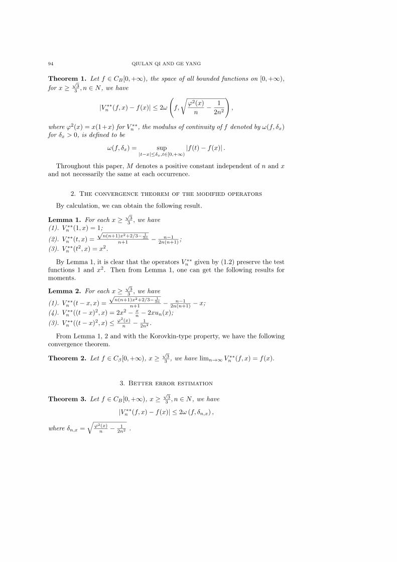
94 QIULAN QI AND GE YANG
Theorem 1. Let f ∈ CB [0,+∞), the space of all bounded functions on [0,+∞),for x ≥
√33 , n ∈ N , we have
|V ∗∗n (f, x)− f(x)| ≤ 2ω
(f,
√ϕ2(x)
n− 1
2n2
),
where ϕ2(x) = x(1+x) for V ∗∗n , the modulus of continuity of f denoted by ω(f, δx)for δx > 0, is defined to be
ω(f, δx) = sup|t−x|≤δx,t∈[0,+∞)
|f(t)− f(x)| .
Throughout this paper, M denotes a positive constant independent of n and xand not necessarily the same at each occurrence.
2. The convergence theorem of the modified operators
By calculation, we can obtain the following result.
Lemma 1. For each x ≥√33 , we have
(1). V ∗∗n (1, x) = 1;
(2). V ∗∗n (t, x) =
√n(n+1)x2+2/3− 1
3n
n+1 − n−12n(n+1) ;
(3). V ∗∗n (t2, x) = x2.
By Lemma 1, it is clear that the operators V ∗∗n given by (1.2) preserve the testfunctions 1 and x2. Then from Lemma 1, one can get the following results formoments.
Lemma 2. For each x ≥√33 , we have
(1). V ∗∗n (t− x, x) =√n(n+1)x2+2/3− 1
3n
n+1 − n−12n(n+1) − x;
(4). V ∗∗n ((t− x)2, x) = 2x2 − xn − 2xun(x);
(3). V ∗∗n ((t− x)2, x) ≤ ϕ2(x)n − 1
2n2 .
From Lemma 1, 2 and with the Korovkin-type property, we have the followingconvergence theorem.
Theorem 2. Let f ∈ Cβ [0,+∞), x ≥√33 , we have limn→∞ V ∗∗n (f, x) = f(x).
3. Better error estimation
Theorem 3. Let f ∈ CB [0,+∞), x ≥√33 , n ∈ N , we have
|V ∗∗n (f, x)− f(x)| ≤ 2ω (f, δn,x) ,
where δn,x =√
ϕ2(x)n − 1
2n2 .
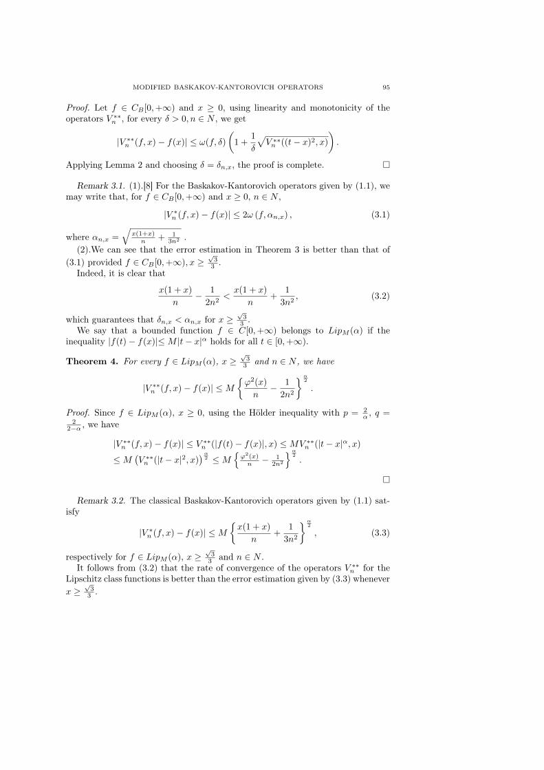
MODIFIED BASKAKOV-KANTOROVICH OPERATORS 95
Proof. Let f ∈ CB [0,+∞) and x ≥ 0, using linearity and monotonicity of theoperators V ∗∗n , for every δ > 0, n ∈ N , we get
|V ∗∗n (f, x)− f(x)| ≤ ω(f, δ)(1 +
1
δ
√V ∗∗n ((t− x)2, x)
).
Applying Lemma 2 and choosing δ = δn,x, the proof is complete.
Remark 3.1. (1).[8] For the Baskakov-Kantorovich operators given by (1.1), wemay write that, for f ∈ CB [0,+∞) and x ≥ 0, n ∈ N ,
|V ∗n (f, x)− f(x)| ≤ 2ω (f, αn,x) , (3.1)
where αn,x =√
x(1+x)n + 1
3n2 .(2).We can see that the error estimation in Theorem 3 is better than that of
(3.1) provided f ∈ CB [0,+∞), x ≥√33 .
Indeed, it is clear that
x(1 + x)
n− 1
2n2<x(1 + x)
n+
1
3n2, (3.2)
which guarantees that δn,x < αn,x for x ≥√33 .
We say that a bounded function f ∈ C[0,+∞) belongs to LipM (α) if theinequality |f(t)− f(x)|≤M |t− x|α holds for all t ∈ [0,+∞).
Theorem 4. For every f ∈ LipM (α), x ≥√33 and n ∈ N , we have
|V ∗∗n (f, x)− f(x)| ≤Mϕ2(x)
n− 1
2n2
α2
.
Proof. Since f ∈ LipM (α), x ≥ 0, using the Hölder inequality with p = 2α , q =
22−α , we have
|V ∗∗n (f, x)− f(x)| ≤ V ∗∗n (|f(t)− f(x)|, x) ≤MV ∗∗n (|t− x|α, x)
≤M(V ∗∗n (|t− x|2, x)
)α2 ≤M
ϕ2(x)n − 1
2n2
α2
.
Remark 3.2. The classical Baskakov-Kantorovich operators given by (1.1) sat-isfy
|V ∗n (f, x)− f(x)| ≤Mx(1 + x)
n+
1
3n2
α2
, (3.3)
respectively for f ∈ LipM (α), x ≥√33 and n ∈ N .
It follows from (3.2) that the rate of convergence of the operators V ∗∗n for theLipschitz class functions is better than the error estimation given by (3.3) wheneverx ≥
√33 .
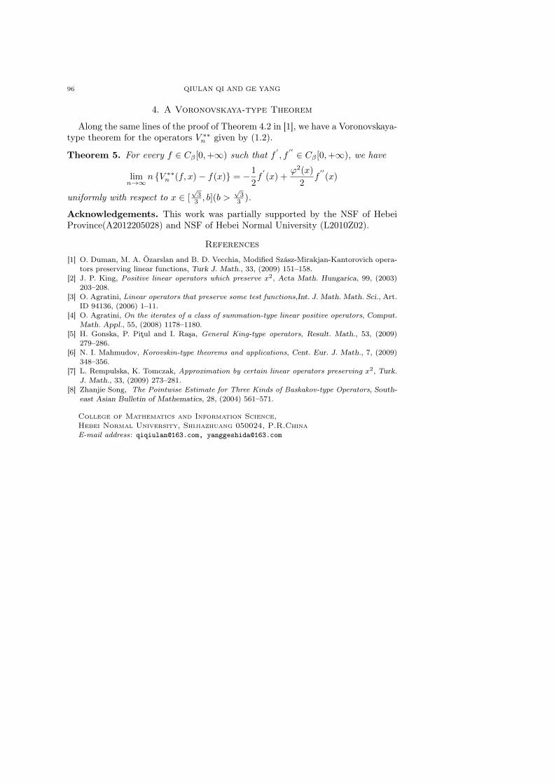
96 QIULAN QI AND GE YANG
4. A Voronovskaya-type Theorem
Along the same lines of the proof of Theorem 4.2 in [1], we have a Voronovskaya-type theorem for the operators V ∗∗n given by (1.2).
Theorem 5. For every f ∈ Cβ [0,+∞) such that f′, f
′′ ∈ Cβ [0,+∞), we have
limn→∞
n V ∗∗n (f, x)− f(x) = −1
2f
′(x) +
ϕ2(x)
2f
′′(x)
uniformly with respect to x ∈ [√33 , b](b >
√33 ).
Acknowledgements. This work was partially supported by the NSF of HebeiProvince(A2012205028) and NSF of Hebei Normal University (L2010Z02).
References
[1] O. Duman, M. A. Özarslan and B. D. Vecchia, Modified Szász-Mirakjan-Kantorovich opera-tors preserving linear functions, Turk J. Math., 33, (2009) 151–158.
[2] J. P. King, Positive linear operators which preserve x2, Acta Math. Hungarica, 99, (2003)203–208.
[3] O. Agratini, Linear operators that preserve some test functions,Int. J. Math. Math. Sci., Art.ID 94136, (2006) 1–11.
[4] O. Agratini, On the iterates of a class of summation-type linear positive operators, Comput.Math. Appl., 55, (2008) 1178–1180.
[5] H. Gonska, P. Piţul and I. Raşa, General King-type operators, Result. Math., 53, (2009)279–286.
[6] N. I. Mahmudov, Korovskin-type theorems and applications, Cent. Eur. J. Math., 7, (2009)348–356.
[7] L. Rempulska, K. Tomczak, Approximation by certain linear operators preserving x2, Turk.J. Math., 33, (2009) 273–281.
[8] Zhanjie Song, The Pointwise Estimate for Three Kinds of Baskakov-type Operators, South-east Asian Bulletin of Mathematics, 28, (2004) 561–571.
College of Mathematics and Information Science,Hebei Normal University, Shijiazhuang 050024, P.R.ChinaE-mail address: [email protected], [email protected]