MATCHING IN CASE CONTROL STUDIES

Matching addresses issues of confounding in the DESIGN stage of a study as opposed to the analysis phase A means of providing a more efficient stratified analysis rather than a direct means of preventing confounding, by increasing precision of estimates (reduction in SE)

Individual Matching

Controls are matched to cases on one or more attributes (i.e. age, gender, smoking status, etc). Each case/control pair then has identical values on the matching factors. Requires a more complex analysis than unmatched data—analytical complexity required to stratify on data not matched on. Each matched set defines it’s own stratum—can be viewed as a single “individual”

Frequency Matching Match on cell instead of individual. Ex. Frequency matching on age and sex. If 20% of cases are 50-54 year old females, than controls are selected in such a way that 20% are also 50-54 years old and female. Does not require using a matched analysis, because you take a random sample of controls in that cell (50-54 year old females). But you have to wait until cases accumulate before controls are selected (unless you know distribution in advance of matching factors)

WHY MATCH? 1. To make control for confounding more efficient when sample size is small Without matching, control for confounding in the analysis will result in many strata with sparse data. By balancing the distribution across strata, the estimates of the OR will be more stable—smaller standard errors, and thus narrower confidence intervals. 2. Even if sample size is not small, if there are many confounders with many categories, data can be sparse in any given stratum. However, you may be able to use multivariate analysis instead. 3. If obtaining information from subjects is expensive. i.e running expensive lab tests on blood samples. Matching will insure control of confounding and will not lead to loss of information. If cost of matching is small compared to cost of expanding study size, matching is worthwhile. 4. Sometimes control of confounding only possible by matching—i.e., controlling for sibship. Alternatives to matching: frequency matching, use multivariate analyses to control confounding

DISADVANTAGES OF MATCHING

Time consuming Can be expensive Can’t always find an exact match Matching can decrease study efficiency because the effort expanded in finding matched subjects could be spent on gathering information for a greater number of unmatched subjects.

Matching Criteria

Matching will increase efficiency only if the matching variables are associated with both the disease and the exposure. The matching variable must also NOT be on the causal chain, i.e. if high fat diet is an exposure of interest, don’t match on high cholesterol or vice versa. If matching is used, matched analysis must be used to take advantage of the matching. If matching was done appropriately, and matching is not taken into account in the analysis, the OR will be biased towards the null. Matching allows you to assess the relationship to exposure and disease having already taken the confounding variable(s) into account, so you don’t need to adjust for these variables in the analysis.

AVOID OVERMATCHING

Term originally referred to “loss of validity in a case control study stemming from a control group that was so closely matched to the case group that the exposure distributions differed very little.” (Rothman, Modern Epidemiology)

Once you match on a factor, you can NOT analyze this factor in the analysis. You have to be assured that you do NOT want to assess the relationship of this factor to the disease. If you match on a variable that is associated with another variable of interest, you will have essentially matched on both of these variables. Example: If you match on neighborhood (i.e census tract), you may also be matching on SES, if neighborhood is correlated with SES. So you would NOT be able to analyze SES as a potential “exposure” variable because you have made the cases and controls the same on this variable. Ex. If female controls are matched to female cases, and vice-vers, you can NOT assess the role of gender on disease because you’ve made cases, controls similar on this variable. If you match on smoking status, you cannot assess the role of this factor in disease. In effect, you are matching on this factor to control confounding for this factor. But you are not concerned about assessing the impact of this factor on the disease.

MORE RECENT INTEPRETATIONS OF OVERMATCHING

CONCERNS WITH EFFICIENCY, NOT VALIDITY Matching can result in LESS information if the expense of matching reduces the total number of study subjects. Study efficiency: Total information content of data/ total number of subjects Cost efficiency: Total information content of data/costs of study

CONTROLS SIMILAR TO CASES ON EXPOSURE WILL NOT CONTRIBUTE TO THE ANALYSIS—loss of efficiency Unnecessary matching— IF MATCHING FACTOR IS ASSOCIATED WITH DISEASE BUT NOT EXPOSURE, MATCHED ANALYSIS WILL BE STATISTICALLY LESS EFFICIENT IF MATCHING FACTOR IS ASSOCIATED WITH EXPOSURE BUT NOT DISEASE, MUST USE MATCHED ANALYSIS, OTHERWISE ODDS RATIO WILL BE BIASED TOWARDS NULL IN UNMATCHED ANALYSIS. BUT VARIANCE OF ODDS RATIO WILL BE INCREASED COMPARED TO UNMATCHED ANALYSIS OF SAME SAMPLE SIZE.

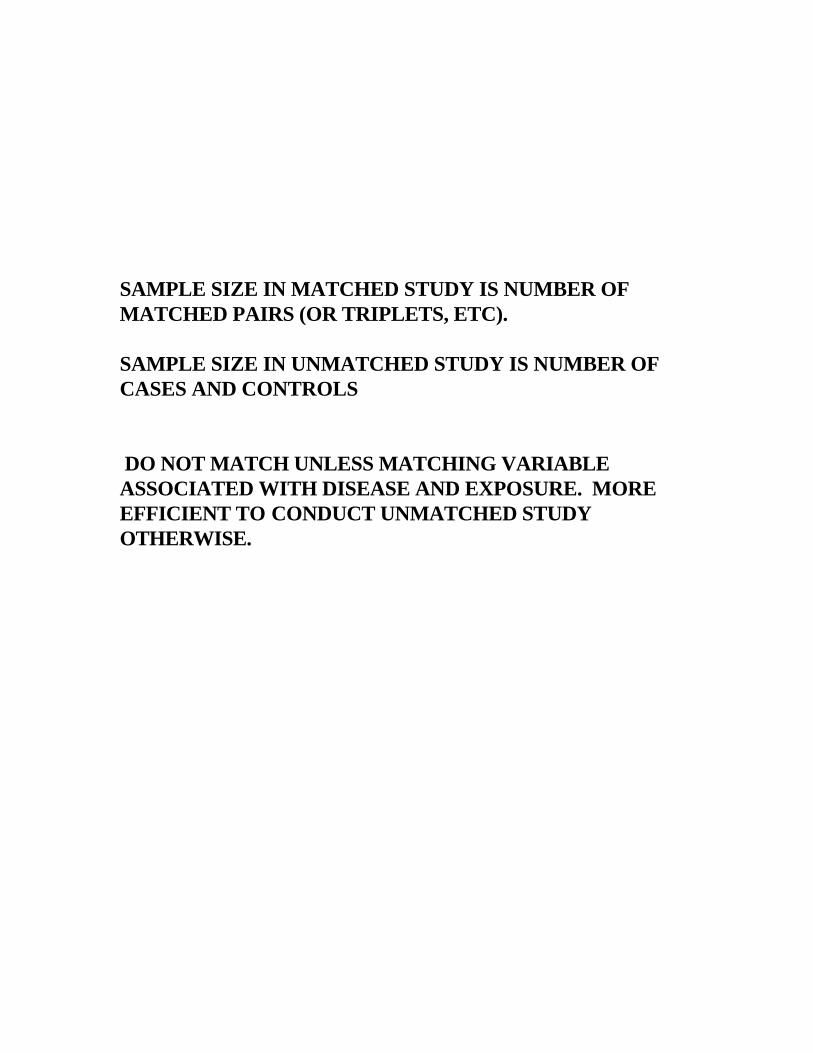
SAMPLE SIZE IN MATCHED STUDY IS NUMBER OF MATCHED PAIRS (OR TRIPLETS, ETC). SAMPLE SIZE IN UNMATCHED STUDY IS NUMBER OF CASES AND CONTROLS DO NOT MATCH UNLESS MATCHING VARIABLE ASSOCIATED WITH DISEASE AND EXPOSURE. MORE EFFICIENT TO CONDUCT UNMATCHED STUDY OTHERWISE.

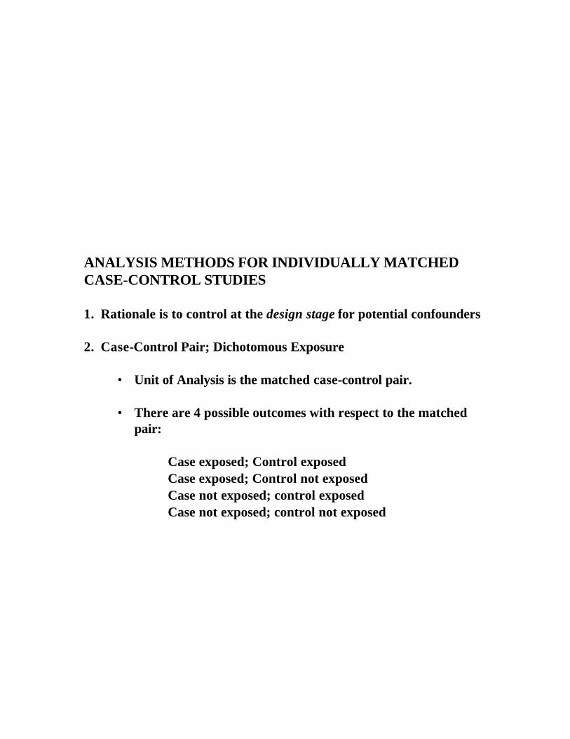
ANALYSIS METHODS FOR INDIVIDUALLY MATCHED CASE-CONTROL STUDIES

1. Rationale is to control at the design stage for potential confounders 2. Case-Control Pair; Dichotomous Exposure

• Unit of Analysis is the matched case-control pair. • There are 4 possible outcomes with respect to the matched

pair:

⇒ Case exposed; Control exposed ⇒ Case exposed; Control not exposed ⇒ Case not exposed; control exposed ⇒ Case not exposed; control not exposed

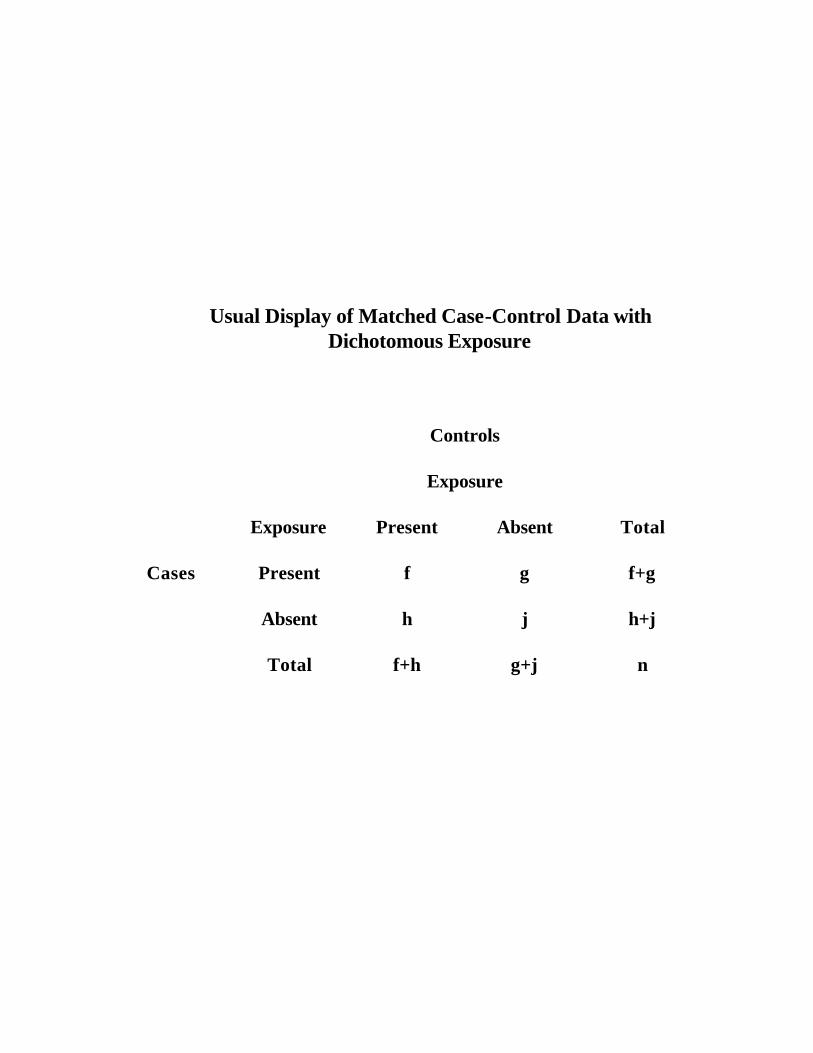
Usual Display of Matched Case-Control Data with Dichotomous Exposure

Controls

Exposure

Exposure Present Absent Total

Cases Present

f g f+g

Absent

h j h+j

Total

f+h g+j n

ODDS RATIO FOR MATCHED PAIR DICHOTOMOUS EXPOSURE CASE-CONTROL STUDIES

OR g h= /

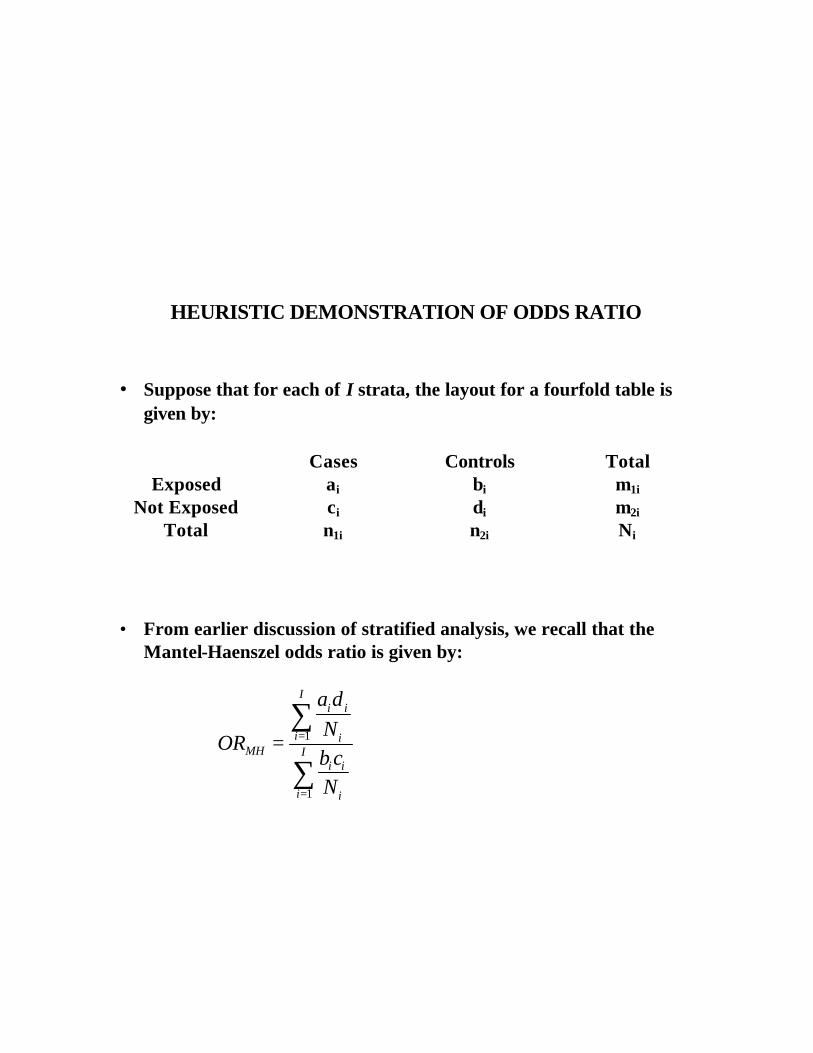
HEURISTIC DEMONSTRATION OF ODDS RATIO • Suppose that for each of I strata, the layout for a fourfold table is

given by:

Cases Controls Total Exposed ai bi m1i

Not Exposed ci di m2i Total n1i n2i Ni

• From earlier discussion of stratified analysis, we recall that the

Mantel-Haenszel odds ratio is given by:

1

1

Ii i

i iMH I

i i

i i

a dN

ORb cN

=

=

=∑

∑

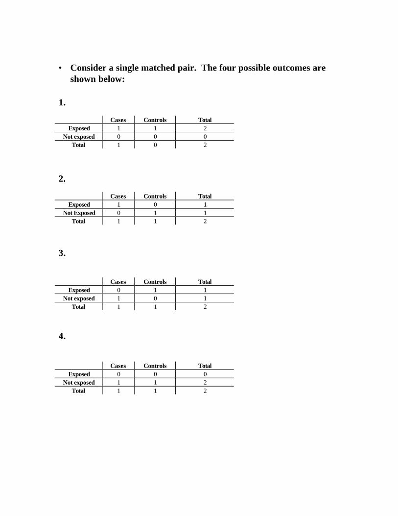
• Consider a single matched pair. The four possible outcomes are

shown below: 1.

Cases Controls Total Exposed 1 1 2

Not exposed 0 0 0 Total 1 0 2

2.

Cases Controls Total Exposed 1 0 1

Not Exposed 0 1 1 Total 1 1 2

3.

Cases Controls Total Exposed 0 1 1

Not exposed 1 0 1 Total 1 1 2

4.

Cases Controls Total Exposed 0 0 0

Not exposed 1 1 2 Total 1 1 2

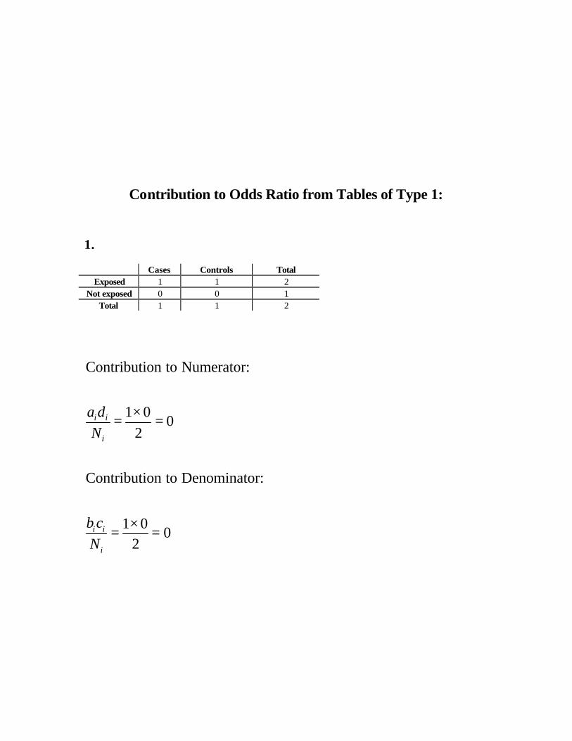
Contribution to Odds Ratio from Tables of Type 1: 1.

Cases Controls Total Exposed 1 1 2

Not exposed 0 0 1 Total 1 1 2

Contribution to Numerator:

1 00

2

Contribution to Denominator:

1 00

2

i i

i

i i

i

a dN

b cN

×= =

×= =

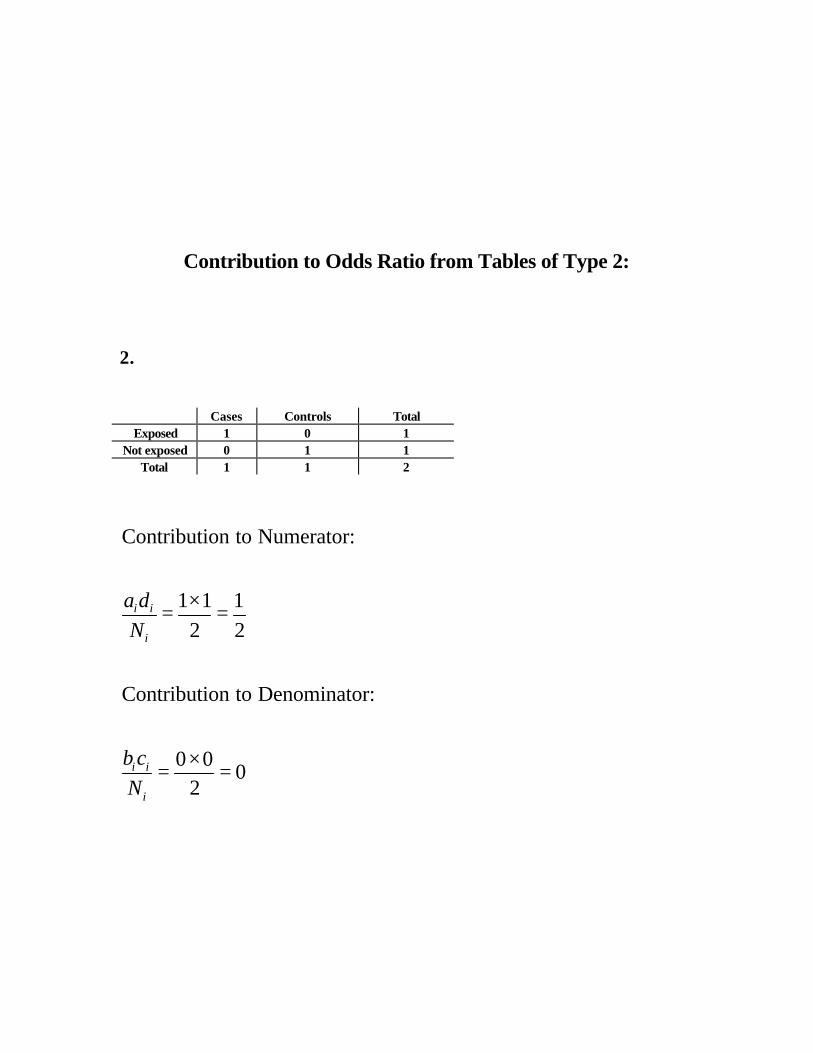
Contribution to Odds Ratio from Tables of Type 2: 2.

Cases Controls Total Exposed 1 0 1

Not exposed 0 1 1 Total 1 1 2

Contribution to Numerator:

1 1 12 2

Contribution to Denominator:

0 00

2

i i

i

i i

i

a dN

b cN

×= =

×= =

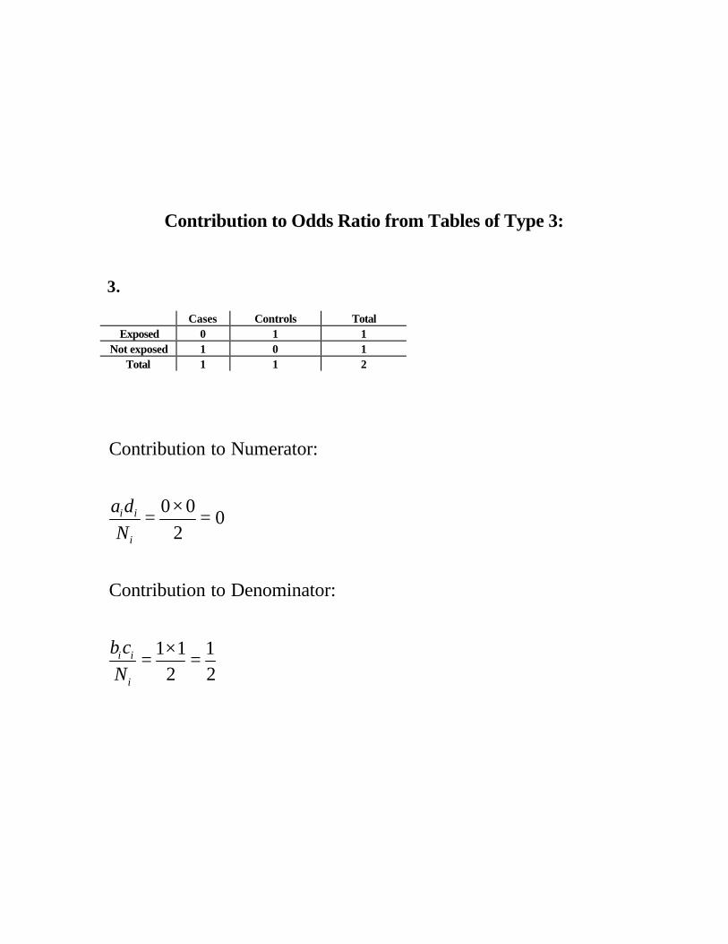
Contribution to Odds Ratio from Tables of Type 3:

3.

Cases Controls Total Exposed 0 1 1

Not exposed 1 0 1 Total 1 1 2

Contribution to Numerator:

0 00

2

Contribution to Denominator:

1 1 12 2

i i

i

i i

i

a dN

b cN

×= =

×= =

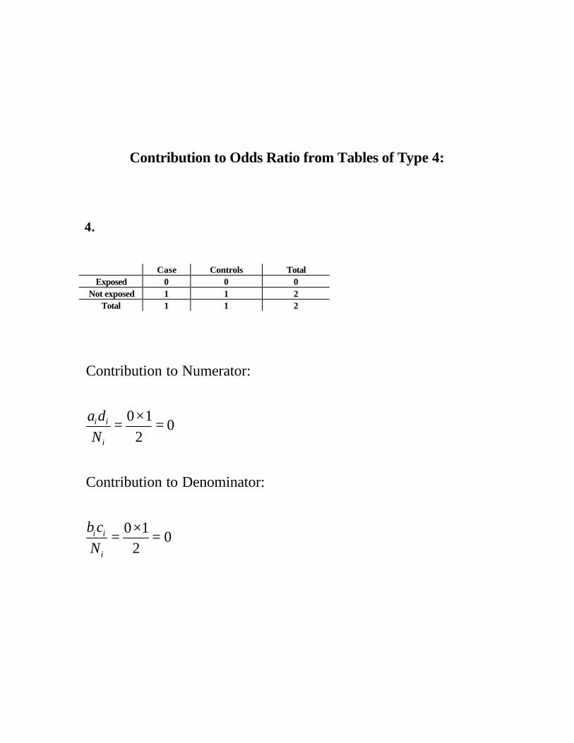
Contribution to Odds Ratio from Tables of Type 4:

4.

Case Controls Total Exposed 0 0 0

Not exposed 1 1 2 Total 1 1 2

Contribution to Numerator:

0 10

2

Contribution to Denominator:

0 10

2

i i

i

i i

i

a dN

b cN

×= =

×= =

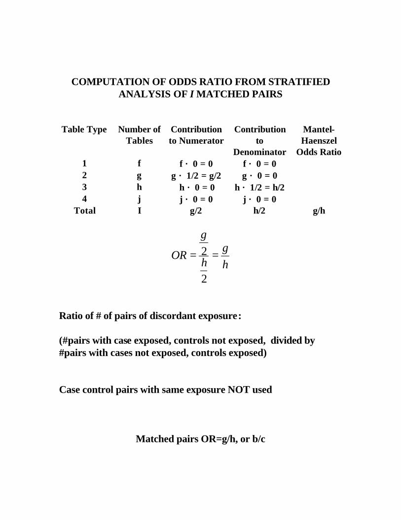
COMPUTATION OF ODDS RATIO FROM STRATIFIED ANALYSIS OF I MATCHED PAIRS

Table Type

Number of Tables

Contribution to Numerator

Contribution to

Denominator

Mantel-Haenszel

Odds Ratio 1 f f × 0 = 0 f × 0 = 0 2 g g × 1/2 = g/2 g × 0 = 0 3 h h × 0 = 0 h × 1/2 = h/2 4 j j × 0 = 0 j × 0 = 0

Total I g/2 h/2 g/h

2

2

gg

ORh h

= =

Ratio of # of pairs of discordant exposure: (#pairs with case exposed, controls not exposed, divided by #pairs with cases not exposed, controls exposed) Case control pairs with same exposure NOT used

Matched pairs OR=g/h, or b/c

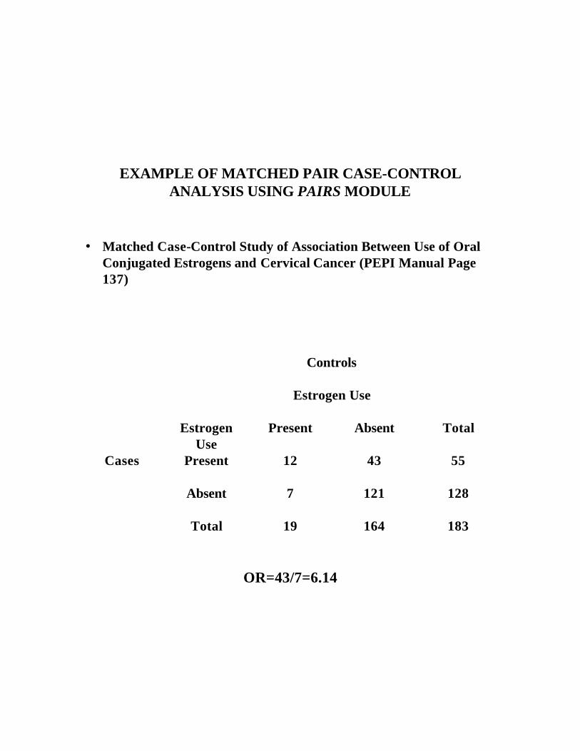
EXAMPLE OF MATCHED PAIR CASE-CONTROL ANALYSIS USING PAIRS MODULE

• Matched Case-Control Study of Association Between Use of Oral Conjugated Estrogens and Cervical Cancer (PEPI Manual Page 137)

Controls

Estrogen Use

Estrogen Use

Present Absent Total

Cases Present

12 43 55

Absent

7 121 128

Total

19 164 183

OR=43/7=6.14

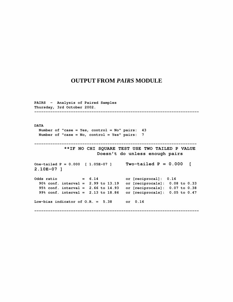
OUTPUT FROM PAIRS MODULE

PAIRS - Analysis of Paired Samples Thursday, 3rd October 2002. ------------------------------------------------------------------------ DATA Number of "case = Yes, control = No" pairs: 43 Number of "case = No, control = Yes" pairs: 7 ----------------------------------------------------------------------- **IF NO CHI SQUARE TEST USE TWO TAILED P VALUE Doesn’t do unless enough pairs One-tailed P = 0.000 [ 1.05E-07 ] Two-tailed P = 0.000 [ 2.10E-07 ] Odds ratio = 6.14 or [reciprocal]: 0.16 90% conf. interval = 2.99 to 13.19 or [reciprocals]: 0.08 to 0.33 95% conf. interval = 2.66 to 14.93 or [reciprocals]: 0.07 to 0.38 99% conf. interval = 2.13 to 18.86 or [reciprocals]: 0.05 to 0.47 Low-bias indicator of O.R. = 5.38 or 0.16 ------------------------------------------------------------------------

SIGNIFICANCE TEST USED IS McNEMAR’S TEST One Degree of Freedom Chi Square Test

p.442 Szklo

( )22

1

| | 1df

g hg h

χ− −

=+

FOR THIS EXAMPLE

( )2

2 43 7 124.5

43 7MCNEMARχ− −

= =+

APPROXIMATE CONFIDENCE INTERVALS FOR MATCHED Odds Ratios (p.442 Szklo)

SE (ln OR)= 1 1b c

+

95% CI(ln OR)=ln OR [ ]( )1.96 lnSE OR± ×

For 95% CI for OR take exponent

95%CI (OR)=exp ( ) 1 1ln 1.96ORb c

± × +

FOR THIS EXAMPLE:

Exp 1 1ln(6.14) 1.9643 7

± × +

= 2.76 - 13.64

(PEPI gives slightly different CI (2.66-14.93) —uses exact methods)

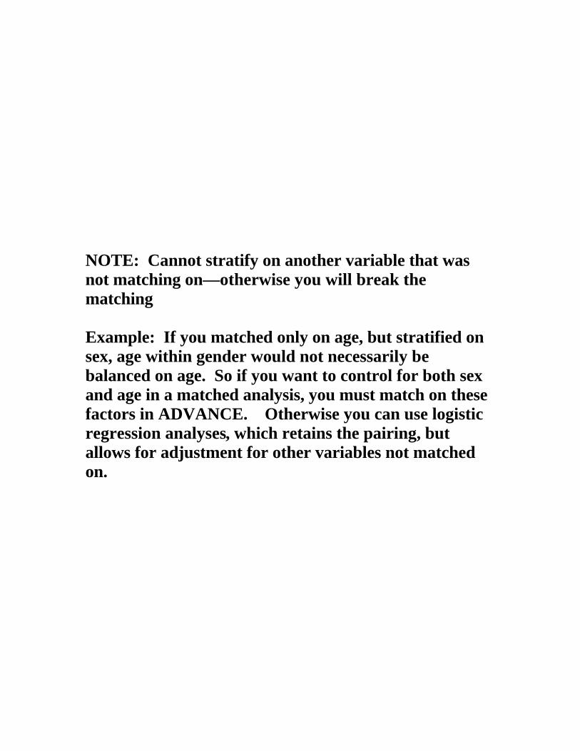
NOTE: Cannot stratify on another variable that was not matching on—otherwise you will break the matching Example: If you matched only on age, but stratified on sex, age within gender would not necessarily be balanced on age. So if you want to control for both sex and age in a matched analysis, you must match on these factors in ADVANCE. Otherwise you can use logistic regression analyses, which retains the pairing, but allows for adjustment for other variables not matched on.

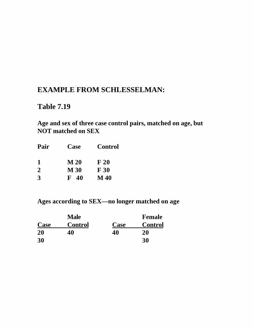
EXAMPLE FROM SCHLESSELMAN: Table 7.19 Age and sex of three case control pairs, matched on age, but NOT matched on SEX Pair Case Control 1 M 20 F 20 2 M 30 F 30 3 F 40 M 40 Ages according to SEX—no longer matched on age Male Female Case Control Case Control 20 40 40 20 30 30

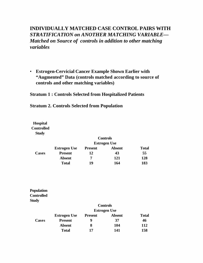
INDIVIDUALLY MATCHED CASE CONTROL PAIRS WITH STRATIFICATION on ANOTHER MATCHING VARIABLE—Matched on Source of controls in addition to other matching variables

• Estrogen-Cervicial Cancer Example Shown Earlier with

“Augmented” Data (controls matched according to source of controls and other matching variables)

Stratum 1 : Controls Selected from Hospitalized Patients Stratum 2. Controls Selected from Population

Hospital

Controlled Study

Controls Estrogen Use Estrogen Use Present Absent Total

Cases Present 12 43 55 Absent 7 121 128 Total

19 164 183

Population Controlled Study

Controls Estrogen Use Estrogen Use Present Absent Total

Cases Present 9 37 46 Absent 8 104 112 Total

17 141 158

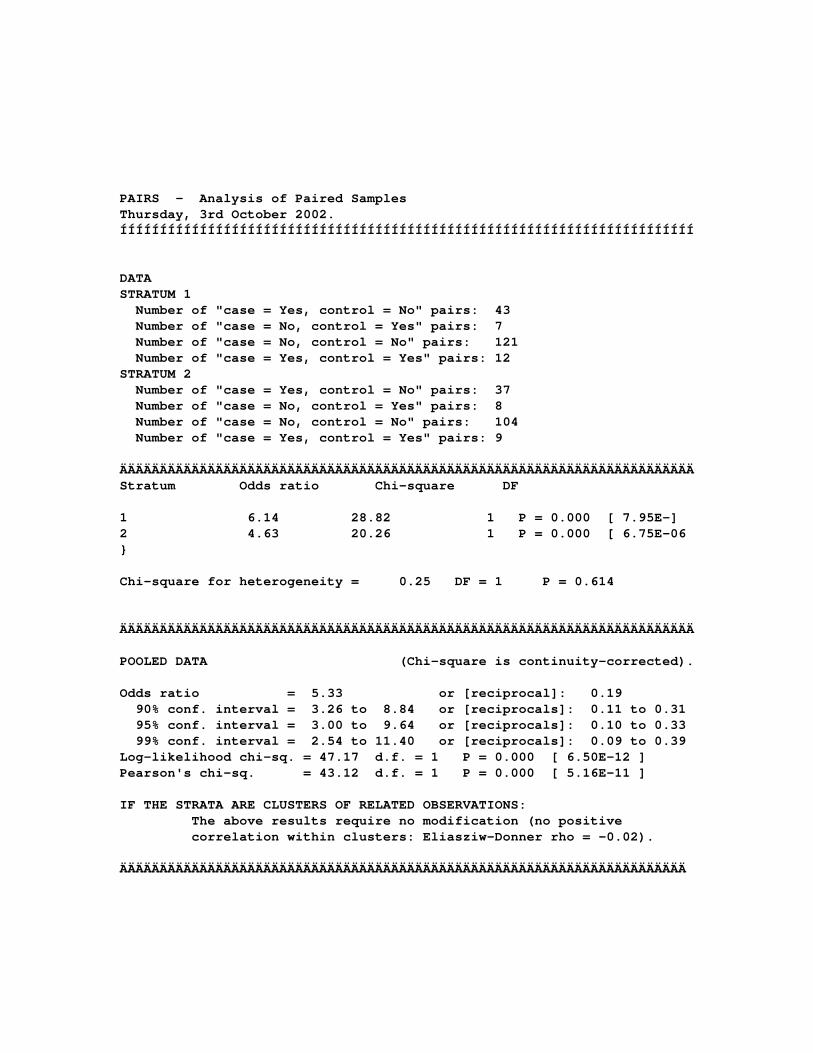
PAIRS - Analysis of Paired Samples Thursday, 3rd October 2002. ÍÍÍÍÍÍÍÍÍÍÍÍÍÍÍÍÍÍÍÍÍÍÍÍÍÍÍÍÍÍÍÍÍÍÍÍÍÍÍÍÍÍÍÍÍÍÍÍÍÍÍÍÍÍÍÍÍÍÍÍÍÍÍÍÍÍÍÍÍÍÍÍ DATA STRATUM 1 Number of "case = Yes, control = No" pairs: 43 Number of "case = No, control = Yes" pairs: 7 Number of "case = No, control = No" pairs: 121 Number of "case = Yes, control = Yes" pairs: 12 STRATUM 2 Number of "case = Yes, control = No" pairs: 37 Number of "case = No, control = Yes" pairs: 8 Number of "case = No, control = No" pairs: 104 Number of "case = Yes, control = Yes" pairs: 9 ÄÄÄÄÄÄÄÄÄÄÄÄÄÄÄÄÄÄÄÄÄÄÄÄÄÄÄÄÄÄÄÄÄÄÄÄÄÄÄÄÄÄÄÄÄÄÄÄÄÄÄÄÄÄÄÄÄÄÄÄÄÄÄÄÄÄÄÄÄÄÄÄ Stratum Odds ratio Chi-square DF 1 6.14 28.82 1 P = 0.000 [ 7.95E-] 2 4.63 20.26 1 P = 0.000 [ 6.75E-06 } Chi-square for heterogeneity = 0.25 DF = 1 P = 0.614 ÄÄÄÄÄÄÄÄÄÄÄÄÄÄÄÄÄÄÄÄÄÄÄÄÄÄÄÄÄÄÄÄÄÄÄÄÄÄÄÄÄÄÄÄÄÄÄÄÄÄÄÄÄÄÄÄÄÄÄÄÄÄÄÄÄÄÄÄÄÄÄÄ POOLED DATA (Chi-square is continuity-corrected). Odds ratio = 5.33 or [reciprocal]: 0.19 90% conf. interval = 3.26 to 8.84 or [reciprocals]: 0.11 to 0.31 95% conf. interval = 3.00 to 9.64 or [reciprocals]: 0.10 to 0.33 99% conf. interval = 2.54 to 11.40 or [reciprocals]: 0.09 to 0.39 Log-likelihood chi-sq. = 47.17 d.f. = 1 P = 0.000 [ 6.50E-12 ] Pearson's chi-sq. = 43.12 d.f. = 1 P = 0.000 [ 5.16E-11 ] IF THE STRATA ARE CLUSTERS OF RELATED OBSERVATIONS: The above results require no modification (no positive correlation within clusters: Eliasziw-Donner rho = -0.02). ÄÄÄÄÄÄÄÄÄÄÄÄÄÄÄÄÄÄÄÄÄÄÄÄÄÄÄÄÄÄÄÄÄÄÄÄÄÄÄÄÄÄÄÄÄÄÄÄÄÄÄÄÄÄÄÄÄÄÄÄÄÄÄÄÄÄÄÄÄÄÄ

CAN MATCH MORE THAN ONE CONTROL PER CASE TO INCREASE PRECISION OF THE ODDS RATIO

(DECREASE STANDARD ERROR)

GIVEN FIXED NUMBER OF CASES, PRECISION OF ODDS RATIO ESTIMATE DECLINES CONSIDERABLY FOR 5 OR MORE CONTROLS PER CASE In other words, the increase in precision when matching 5 or more cases is minimal, and not worth the extra expense and resources required to conduct the matching.

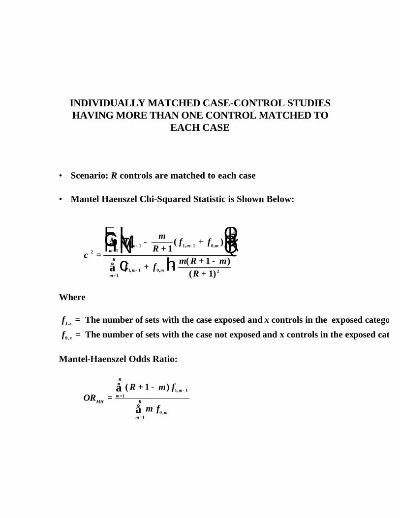
INDIVIDUALLY MATCHED CASE-CONTROL STUDIES HAVING MORE THAN ONE CONTROL MATCHED TO

EACH CASE

• Scenario: R controls are matched to each case • Mantel Haenszel Chi-Squared Statistic is Shown Below:

χ 21 1 1 1 0

1

2

1 1 0 21

111

=−

++L

NMOQP

FHG

IKJ

+ ×+ −+

− −=

−=

∑

∑

fm

Rf f

f fm R m

R

m m mm

R

m mm

R

, , ,

, ,

( )

( )( )

c h

Where f x

fx

x

1

0

,

,

= The number of sets with the case exposed and controls in the exposed category.

= The number of sets with the case not exposed and x controls in the exposed cate

Mantel-Haenszel Odds Ratio:

ORR m f

m fMH

mm

R

mm

R=+ − −

=

=

∑

∑

( ) ,

,

1 1 11

01

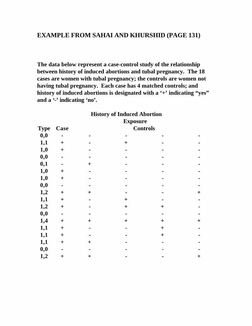
EXAMPLE FROM SAHAI AND KHURSHID (PAGE 131)

The data below represent a case-control study of the relationship between history of induced abortions and tubal pregnancy. The 18 cases are women with tubal pregnancy; the controls are women not having tubal pregnancy. Each case has 4 matched controls; and history of induced abortions is designated with a ‘+’ indicating “yes” and a ‘-’ indicating ‘no’.

History of Induced Abortion Exposure

Type Case Controls 0,0 - - - - - 1,1 + - + - - 1,0 + - - - - 0,0 - - - - - 0,1 - + - - - 1,0 + - - - - 1,0 + - - - - 0,0 - - - - - 1,2 + + - - + 1,1 + - + - - 1,2 + - + + - 0,0 - - - - - 1,4 + + + + + 1,1 + - - + - 1,1 + - - + - 1,1 + + - - - 0,0 - - - - - 1,2 + + - - +

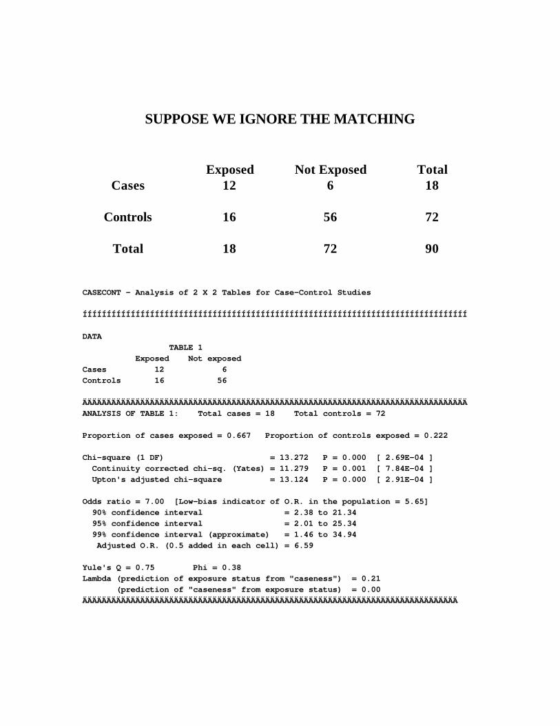
SUPPOSE WE IGNORE THE MATCHING

Exposed Not Exposed Total Cases

12 6 18

Controls

16 56 72

Total 18 72 90

CASECONT - Analysis of 2 X 2 Tables for Case-Control Studies ÍÍÍÍÍÍÍÍÍÍÍÍÍÍÍÍÍÍÍÍÍÍÍÍÍÍÍÍÍÍÍÍÍÍÍÍÍÍÍÍÍÍÍÍÍÍÍÍÍÍÍÍÍÍÍÍÍÍÍÍÍÍÍÍÍÍÍÍÍÍÍÍÍÍÍÍÍÍÍÍ DATA TABLE 1 Exposed Not exposed Cases 12 6 Controls 16 56 ÄÄÄÄÄÄÄÄÄÄÄÄÄÄÄÄÄÄÄÄÄÄÄÄÄÄÄÄÄÄÄÄÄÄÄÄÄÄÄÄÄÄÄÄÄÄÄÄÄÄÄÄÄÄÄÄÄÄÄÄÄÄÄÄÄÄÄÄÄÄÄÄÄÄÄÄÄÄÄÄ ANALYSIS OF TABLE 1: Total cases = 18 Total controls = 72 Proportion of cases exposed = 0.667 Proportion of controls exposed = 0.222 Chi-square (1 DF) = 13.272 P = 0.000 [ 2.69E-04 ] Continuity corrected chi-sq. (Yates) = 11.279 P = 0.001 [ 7.84E-04 ] Upton's adjusted chi-square = 13.124 P = 0.000 [ 2.91E-04 ] Odds ratio = 7.00 [Low-bias indicator of O.R. in the population = 5.65] 90% confidence interval = 2.38 to 21.34 95% confidence interval = 2.01 to 25.34 99% confidence interval (approximate) = 1.46 to 34.94 Adjusted O.R. (0.5 added in each cell) = 6.59 Yule's Q = 0.75 Phi = 0.38 Lambda (prediction of exposure status from "caseness") = 0.21 (prediction of "caseness" from exposure status) = 0.00 ÄÄÄÄÄÄÄÄÄÄÄÄÄÄÄÄÄÄÄÄÄÄÄÄÄÄÄÄÄÄÄÄÄÄÄÄÄÄÄÄÄÄÄÄÄÄÄÄÄÄÄÄÄÄÄÄÄÄÄÄÄÄÄÄÄÄÄÄÄÄÄÄÄÄÄÄÄÄ

RATIONALE FOR MATCHED CHI-SQUARED STATISTIC

• As with paired data, let us consider each matched set of 1 case and

R controls as a single “stratum” which would yield the following fourfold table(NOTE CASE-CONTROL/EXPOSURE order reversed to be consistent with PEPI modules):

Exposed Not Exposed Total

Cases y 1 - y 1 Controls x R - x R

Total x + y R + 1 - (x + y) R + 1

Note: y = 0 or 1 (Only one case, either exposed or not exposed)

• We can then compute the Mantel-Haenszel test and odds ratios as we do for a stratified analysis .

• The tables having x = 0 and y = 0; and x = R and y = 1 are “non-

informative” analogous to what we saw for the individually 1 to 1 matched case-control design.

• The Mantel-Haenszel test and odds ratio can then be calculated in

the usual stratified analysis way (e.g., using the CASECONT module).

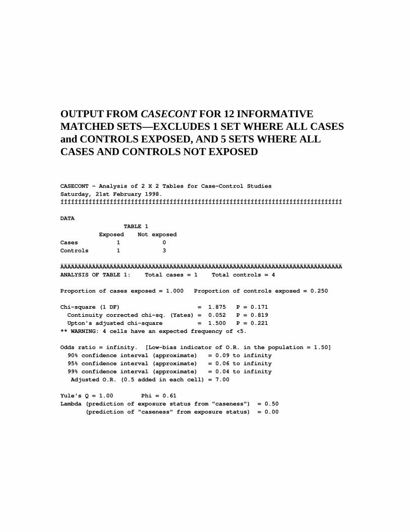
OUTPUT FROM CASECONT FOR 12 INFORMATIVE MATCHED SETS—EXCLUDES 1 SET WHERE ALL CASES and CONTROLS EXPOSED, AND 5 SETS WHERE ALL CASES AND CONTROLS NOT EXPOSED

CASECONT - Analysis of 2 X 2 Tables for Case-Control Studies Saturday, 21st February 1998. ÍÍÍÍÍÍÍÍÍÍÍÍÍÍÍÍÍÍÍÍÍÍÍÍÍÍÍÍÍÍÍÍÍÍÍÍÍÍÍÍÍÍÍÍÍÍÍÍÍÍÍÍÍÍÍÍÍÍÍÍÍÍÍÍÍÍÍÍÍÍÍÍÍÍÍÍÍÍÍÍ DATA TABLE 1 Exposed Not exposed Cases 1 0 Controls 1 3 ÄÄÄÄÄÄÄÄÄÄÄÄÄÄÄÄÄÄÄÄÄÄÄÄÄÄÄÄÄÄÄÄÄÄÄÄÄÄÄÄÄÄÄÄÄÄÄÄÄÄÄÄÄÄÄÄÄÄÄÄÄÄÄÄÄÄÄÄÄÄÄÄÄÄÄÄÄÄÄÄ ANALYSIS OF TABLE 1: Total cases = 1 Total controls = 4 Proportion of cases exposed = 1.000 Proportion of controls exposed = 0.250 Chi-square (1 DF) = 1.875 P = 0.171 Continuity corrected chi-sq. (Yates) = 0.052 P = 0.819 Upton's adjusted chi-square = 1.500 P = 0.221 ** WARNING: 4 cells have an expected frequency of <5. Odds ratio = infinity. [Low-bias indicator of O.R. in the population = 1.50] 90% confidence interval (approximate) = 0.09 to infinity 95% confidence interval (approximate) = 0.06 to infinity 99% confidence interval (approximate) = 0.04 to infinity Adjusted O.R. (0.5 added in each cell) = 7.00 Yule's Q = 1.00 Phi = 0.61 Lambda (prediction of exposure status from "caseness") = 0.50 (prediction of "caseness" from exposure status) = 0.00

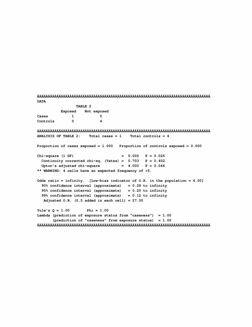
ÄÄÄÄÄÄÄÄÄÄÄÄÄÄÄÄÄÄÄÄÄÄÄÄÄÄÄÄÄÄÄÄÄÄÄÄÄÄÄÄÄÄÄÄÄÄÄÄÄÄÄÄÄÄÄÄÄÄÄÄÄÄÄÄÄÄÄÄÄÄÄÄÄÄÄÄÄÄÄÄ DATA TABLE 2 Exposed Not exposed Cases 1 0 Controls 0 4 ÄÄÄÄÄÄÄÄÄÄÄÄÄÄÄÄÄÄÄÄÄÄÄÄÄÄÄÄÄÄÄÄÄÄÄÄÄÄÄÄÄÄÄÄÄÄÄÄÄÄÄÄÄÄÄÄÄÄÄÄÄÄÄÄÄÄÄÄÄÄÄÄÄÄÄÄÄÄÄÄ ANALYSIS OF TABLE 2: Total cases = 1 Total controls = 4 Proportion of cases exposed = 1.000 Proportion of controls exposed = 0.000 Chi-square (1 DF) = 5.000 P = 0.025 Continuity corrected chi-sq. (Yates) = 0.703 P = 0.402 Upton's adjusted chi-square = 4.000 P = 0.046 ** WARNING: 4 cells have an expected frequency of <5. Odds ratio = infinity. [Low-bias indicator of O.R. in the population = 4.00] 90% confidence interval (approximate) = 0.28 to infinity 95% confidence interval (approximate) = 0.20 to infinity 99% confidence interval (approximate) = 0.12 to infinity Adjusted O.R. (0.5 added in each cell) = 27.00 Yule's Q = 1.00 Phi = 1.00 Lambda (prediction of exposure status from "caseness") = 1.00 (prediction of "caseness" from exposure status) = 1.00 ÄÄÄÄÄÄÄÄÄÄÄÄÄÄÄÄÄÄÄÄÄÄÄÄÄÄÄÄÄÄÄÄÄÄÄÄÄÄÄÄÄÄÄÄÄÄÄÄÄÄÄÄÄÄÄÄÄÄÄÄÄÄÄÄÄÄÄÄÄÄÄÄÄÄÄÄÄÄÄÄ

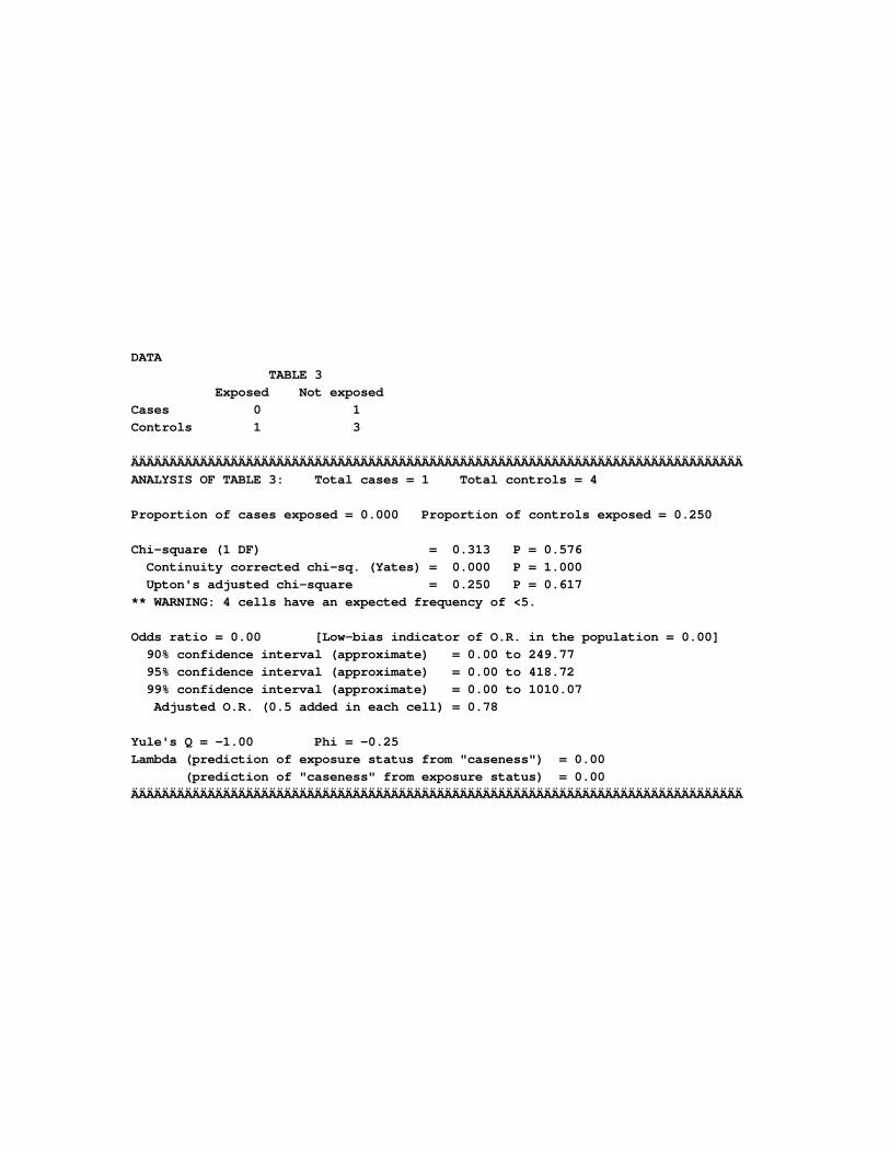
DATA TABLE 3 Exposed Not exposed Cases 0 1 Controls 1 3 ÄÄÄÄÄÄÄÄÄÄÄÄÄÄÄÄÄÄÄÄÄÄÄÄÄÄÄÄÄÄÄÄÄÄÄÄÄÄÄÄÄÄÄÄÄÄÄÄÄÄÄÄÄÄÄÄÄÄÄÄÄÄÄÄÄÄÄÄÄÄÄÄÄÄÄÄÄÄÄÄ ANALYSIS OF TABLE 3: Total cases = 1 Total controls = 4 Proportion of cases exposed = 0.000 Proportion of controls exposed = 0.250 Chi-square (1 DF) = 0.313 P = 0.576 Continuity corrected chi-sq. (Yates) = 0.000 P = 1.000 Upton's adjusted chi-square = 0.250 P = 0.617 ** WARNING: 4 cells have an expected frequency of <5. Odds ratio = 0.00 [Low-bias indicator of O.R. in the population = 0.00] 90% confidence interval (approximate) = 0.00 to 249.77 95% confidence interval (approximate) = 0.00 to 418.72 99% confidence interval (approximate) = 0.00 to 1010.07 Adjusted O.R. (0.5 added in each cell) = 0.78 Yule's Q = -1.00 Phi = -0.25 Lambda (prediction of exposure status from "caseness") = 0.00 (prediction of "caseness" from exposure status) = 0.00 ÄÄÄÄÄÄÄÄÄÄÄÄÄÄÄÄÄÄÄÄÄÄÄÄÄÄÄÄÄÄÄÄÄÄÄÄÄÄÄÄÄÄÄÄÄÄÄÄÄÄÄÄÄÄÄÄÄÄÄÄÄÄÄÄÄÄÄÄÄÄÄÄÄÄÄÄÄÄÄÄ

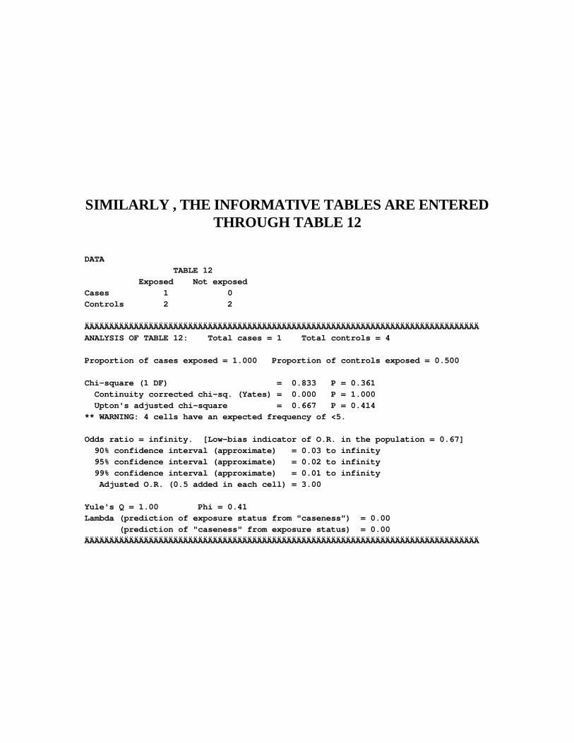
SIMILARLY , THE INFORMATIVE TABLES ARE ENTERED THROUGH TABLE 12

DATA TABLE 12 Exposed Not exposed Cases 1 0 Controls 2 2 ÄÄÄÄÄÄÄÄÄÄÄÄÄÄÄÄÄÄÄÄÄÄÄÄÄÄÄÄÄÄÄÄÄÄÄÄÄÄÄÄÄÄÄÄÄÄÄÄÄÄÄÄÄÄÄÄÄÄÄÄÄÄÄÄÄÄÄÄÄÄÄÄÄÄÄÄÄÄÄÄ ANALYSIS OF TABLE 12: Total cases = 1 Total controls = 4 Proportion of cases exposed = 1.000 Proportion of controls exposed = 0.500 Chi-square (1 DF) = 0.833 P = 0.361 Continuity corrected chi-sq. (Yates) = 0.000 P = 1.000 Upton's adjusted chi-square = 0.667 P = 0.414 ** WARNING: 4 cells have an expected frequency of <5. Odds ratio = infinity. [Low-bias indicator of O.R. in the population = 0.67] 90% confidence interval (approximate) = 0.03 to infinity 95% confidence interval (approximate) = 0.02 to infinity 99% confidence interval (approximate) = 0.01 to infinity Adjusted O.R. (0.5 added in each cell) = 3.00 Yule's Q = 1.00 Phi = 0.41 Lambda (prediction of exposure status from "caseness") = 0.00 (prediction of "caseness" from exposure status) = 0.00 ÄÄÄÄÄÄÄÄÄÄÄÄÄÄÄÄÄÄÄÄÄÄÄÄÄÄÄÄÄÄÄÄÄÄÄÄÄÄÄÄÄÄÄÄÄÄÄÄÄÄÄÄÄÄÄÄÄÄÄÄÄÄÄÄÄÄÄÄÄÄÄÄÄÄÄÄÄÄÄÄ

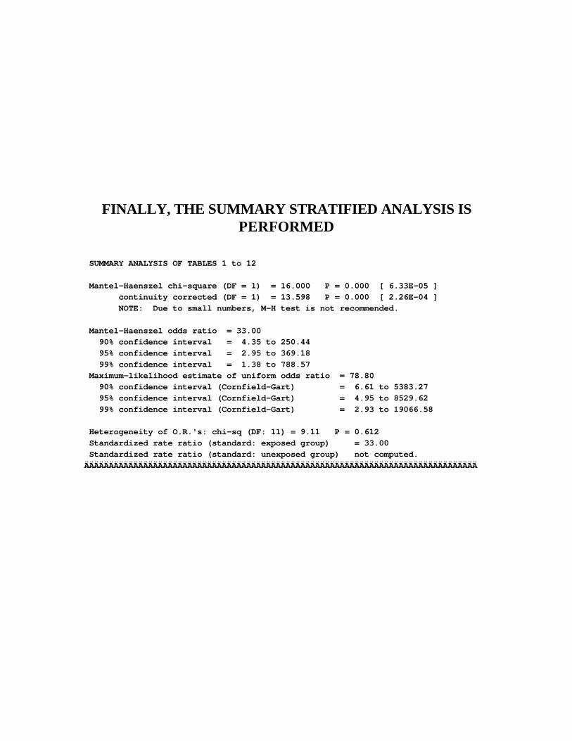
FINALLY, THE SUMMARY STRATIFIED ANALYSIS IS PERFORMED

SUMMARY ANALYSIS OF TABLES 1 to 12 Mantel-Haenszel chi-square (DF = 1) = 16.000 P = 0.000 [ 6.33E-05 ] continuity corrected (DF = 1) = 13.598 P = 0.000 [ 2.26E-04 ] NOTE: Due to small numbers, M-H test is not recommended. Mantel-Haenszel odds ratio = 33.00 90% confidence interval = 4.35 to 250.44 95% confidence interval = 2.95 to 369.18 99% confidence interval = 1.38 to 788.57 Maximum-likelihood estimate of uniform odds ratio = 78.80 90% confidence interval (Cornfield-Gart) = 6.61 to 5383.27 95% confidence interval (Cornfield-Gart) = 4.95 to 8529.62 99% confidence interval (Cornfield-Gart) = 2.93 to 19066.58 Heterogeneity of O.R.'s: chi-sq (DF: 11) = 9.11 P = 0.612 Standardized rate ratio (standard: exposed group) = 33.00 Standardized rate ratio (standard: unexposed group) not computed. ÄÄÄÄÄÄÄÄÄÄÄÄÄÄÄÄÄÄÄÄÄÄÄÄÄÄÄÄÄÄÄÄÄÄÄÄÄÄÄÄÄÄÄÄÄÄÄÄÄÄÄÄÄÄÄÄÄÄÄÄÄÄÄÄÄÄÄÄÄÄÄÄÄÄÄÄÄÄÄÄ

THE FORMULAS STATED EARLIER ARE “SHORTCUTS” TO AVOID HAVING TO ENTER EVERY MATCHED SET AS A SEPARATE TABLE

INSTEAD, TABULATE FREQUENCY OF EXPOSURE OUTCOMES AND ENTER INTO PEPI MODULE “MATCHED” For this example:

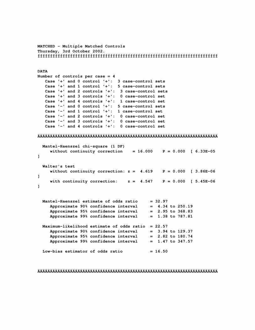
MATCHED - Multiple Matched Controls Thursday, 3rd October 2002. ÍÍÍÍÍÍÍÍÍÍÍÍÍÍÍÍÍÍÍÍÍÍÍÍÍÍÍÍÍÍÍÍÍÍÍÍÍÍÍÍÍÍÍÍÍÍÍÍÍÍÍÍÍÍÍÍÍÍÍÍÍÍÍÍÍÍÍÍÍÍÍÍ DATA Number of controls per case = 4 Case '+' and 0 control '+': 3 case-control sets Case '+' and 1 control '+': 5 case-control sets Case '+' and 2 controls '+': 3 case-control sets Case '+' and 3 controls '+': 0 case-control set Case '+' and 4 controls '+': 1 case-control set Case '-' and 0 control '+': 5 case-control sets Case '-' and 1 control '+': 1 case-control set Case '-' and 2 controls '+': 0 case-control set Case '-' and 3 controls '+': 0 case-control set Case '-' and 4 controls '+': 0 case-control set ÄÄÄÄÄÄÄÄÄÄÄÄÄÄÄÄÄÄÄÄÄÄÄÄÄÄÄÄÄÄÄÄÄÄÄÄÄÄÄÄÄÄÄÄÄÄÄÄÄÄÄÄÄÄÄÄÄÄÄÄÄÄÄÄÄÄÄÄÄÄÄÄ Mantel-Haenszel chi-square (1 DF) without continuity correction = 16.000 P = 0.000 [ 6.33E-05 ] Walter's test without continuity correction: z = 4.619 P = 0.000 [ 3.86E-06 ] with continuity correction: z = 4.547 P = 0.000 [ 5.45E-06 ] Mantel-Haenszel estimate of odds ratio = 32.97 Approximate 90% confidence interval = 4.34 to 250.19 Approximate 95% confidence interval = 2.95 to 368.83 Approximate 99% confidence interval = 1.38 to 787.81 Maximum-likelihood estimate of odds ratio = 22.57 Approximate 90% confidence interval = 3.94 to 129.37 Approximate 95% confidence interval = 2.82 to 180.74 Approximate 99% confidence interval = 1.47 to 347.57 Low-bias estimator of odds ratio = 16.50 ÄÄÄÄÄÄÄÄÄÄÄÄÄÄÄÄÄÄÄÄÄÄÄÄÄÄÄÄÄÄÄÄÄÄÄÄÄÄÄÄÄÄÄÄÄÄÄÄÄÄÄÄÄÄÄÄÄÄÄÄÄÄÄÄÄÄÄÄÄÄÄÄ

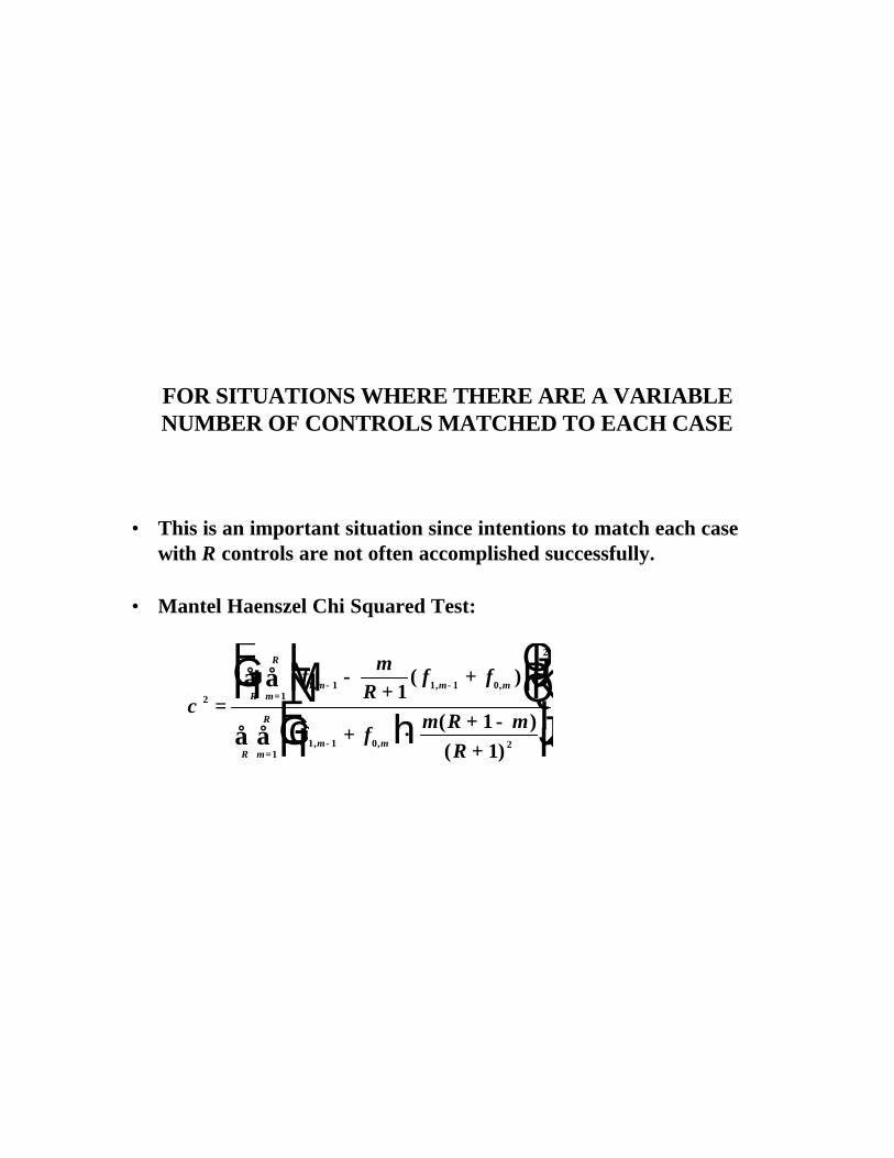
FOR SITUATIONS WHERE THERE ARE A VARIABLE NUMBER OF CONTROLS MATCHED TO EACH CASE

• This is an important situation since intentions to match each case

with R controls are not often accomplished successfully. • Mantel Haenszel Chi Squared Test:

χ 21 1 1 1 0

1

2

1 1 0 21

111

=−

++L

NMOQP

FHG

IKJ

+ ×+ −+

FHG

IKJ

− −=

−=

∑∑

∑∑

fm

Rf f

f fm R m

R

m m mm

R

R

m mm

R

R

, , ,

, ,

( )

( )( )

c h

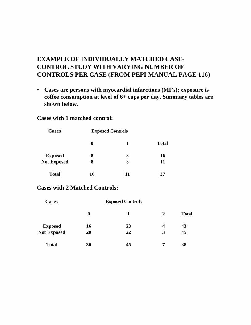
EXAMPLE OF INDIVIDUALLY MATCHED CASE-CONTROL STUDY WITH VARYING NUMBER OF CONTROLS PER CASE (FROM PEPI MANUAL PAGE 116)

• Cases are persons with myocardial infarctions (MI’s); exposure is

coffee consumption at level of 6+ cups per day. Summary tables are shown below.

Cases with 1 matched control:

Cases Exposed Controls

0 1

Total

Exposed 8 8 16 Not Exposed 8 3

11

Total 16 11 27

Cases with 2 Matched Controls:

Cases Exposed Controls

0 1 2

Total

Exposed 16 23 4 43 Not Exposed 20

22 3 45

Total 36 45 7 88

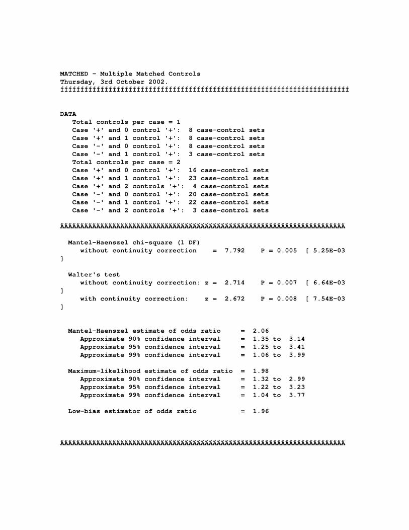
MATCHED - Multiple Matched Controls Thursday, 3rd October 2002. ÍÍÍÍÍÍÍÍÍÍÍÍÍÍÍÍÍÍÍÍÍÍÍÍÍÍÍÍÍÍÍÍÍÍÍÍÍÍÍÍÍÍÍÍÍÍÍÍÍÍÍÍÍÍÍÍÍÍÍÍÍÍÍÍÍÍÍÍÍÍÍÍ DATA Total controls per case = 1 Case '+' and 0 control '+': 8 case-control sets Case '+' and 1 control '+': 8 case-control sets Case '-' and 0 control '+': 8 case-control sets Case '-' and 1 control '+': 3 case-control sets Total controls per case = 2 Case '+' and 0 control '+': 16 case-control sets Case '+' and 1 control '+': 23 case-control sets Case '+' and 2 controls '+': 4 case-control sets Case '-' and 0 control '+': 20 case-control sets Case '-' and 1 control '+': 22 case-control sets Case '-' and 2 controls '+': 3 case-control sets ÄÄÄÄÄÄÄÄÄÄÄÄÄÄÄÄÄÄÄÄÄÄÄÄÄÄÄÄÄÄÄÄÄÄÄÄÄÄÄÄÄÄÄÄÄÄÄÄÄÄÄÄÄÄÄÄÄÄÄÄÄÄÄÄÄÄÄÄÄÄÄ Mantel-Haenszel chi-square (1 DF) without continuity correction = 7.792 P = 0.005 [ 5.25E-03 ] Walter's test without continuity correction: z = 2.714 P = 0.007 [ 6.64E-03 ] with continuity correction: z = 2.672 P = 0.008 [ 7.54E-03 ] Mantel-Haenszel estimate of odds ratio = 2.06 Approximate 90% confidence interval = 1.35 to 3.14 Approximate 95% confidence interval = 1.25 to 3.41 Approximate 99% confidence interval = 1.06 to 3.99 Maximum-likelihood estimate of odds ratio = 1.98 Approximate 90% confidence interval = 1.32 to 2.99 Approximate 95% confidence interval = 1.22 to 3.23 Approximate 99% confidence interval = 1.04 to 3.77 Low-bias estimator of odds ratio = 1.96 ÄÄÄÄÄÄÄÄÄÄÄÄÄÄÄÄÄÄÄÄÄÄÄÄÄÄÄÄÄÄÄÄÄÄÄÄÄÄÄÄÄÄÄÄÄÄÄÄÄÄÄÄÄÄÄÄÄÄÄÄÄÄÄÄÄÄÄÄÄÄÄ