MAT187H1F Lec0101 Burbulla - math.utoronto.ca · Chapter 11: Parametric and Polar Curves MAT187H1F Lec0101 Burbulla Chapter 11 Lecture Notes Spring 2017 Chapter 11 Lecture Notes MAT187H1F

Chapter 11: Parametric and Polar Curves

MAT187H1F Lec0101 Burbulla

Chapter 11 Lecture Notes

Spring 2017

Chapter 11 Lecture Notes MAT187H1F Lec0101 Burbulla

Chapter 11: Parametric and Polar Curves

Chapter 11: Parametric and Polar Curves11.1 Parametric Equations11.2 Polar Coordinates11.3 Calculus in Polar Coordinates



What Is A Parametric Curve?

x

y

rP(x , y)

1. Let a point P on a curve haveCartesian coordinates (x , y)

2. We can think of the curve asbeing traced out as the pointP moves along it.

3. In this way we can think ofboth x and y as functions of t.

4. x = f (t) and y = g(t) arecalled parametric equations ofthe curve; t is called aparameter.



Example 1

Figure: The circle x2 + y2 = 1

Let {x = cos ty = sin t

with 0 ≤ t ≤ 2π. These areparametric equations of a cir-cle:

x2 + y2 = cos2 t + sin2 t = 1.

In terms of t, the circle is beingtraced out counter clockwise.



Example 2

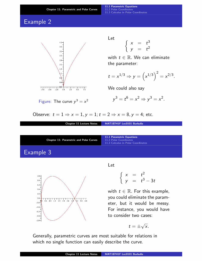
Figure: The curve y3 = x2

Let {x = t3

y = t2

with t ∈ R. We can eliminatethe parameter:

t = x1/3 ⇒ y =(x1/3

)2= x2/3.

We could also say

y3 = t6 = x2 ⇒ y3 = x2.

Observe: t = 1⇒ x = 1, y = 1; t = 2⇒ x = 8, y = 4; etc.



Example 3

Let {x = t2

y = t3 − 3t

with t ∈ R. For this example,you could eliminate the param-eter, but it would be messy.For instance, you would haveto consider two cases:

t = ±√

x .

Generally, parametric curves are most suitable for relations inwhich no single function can easily describe the curve.



Most General Form of a Curve

Parametric curves are the most general type of curve. The functiony = f (x) can be described parametrically by{

x = ty = f (t)

, t a parameter

In essence, x is the parameter of a curve described by the functiony = f (x). All curves we shall look at later, polar curves and curvesin 3 dimensions, can be described parametrically.



Derivatives of Parametric Curves

To do calculus with parametric curves we will need formulas forderivatives in terms of the parameter. Suppose x and y arefunctions of a parameter t. Then

dy

dt=

dy

dx

dx

dt⇒ dy

dx=

dy

dtdx

dt

As always, the derivative will be the slope of the curve at thepoint (x , y); the difference is that everything will be calculated interms of the parameter t.



Example 4; Example 2 Revisited

We have x = t3, y = t2; so

dy

dx=

dy

dtdx

dt

=2t

3t2=

2

3t, t 6= 0.

This is the same answer you get if you eliminate the parameter:

t = x1/3 ⇒ y = x2/3 ⇒ dy

dx=

2

3x−1/3.



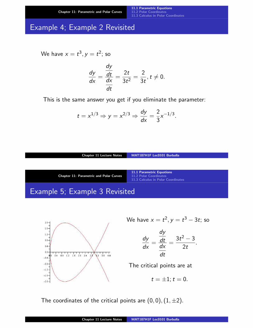
Example 5; Example 3 Revisited

We have x = t2, y = t3 − 3t; so

dy

dx=

dy

dtdx

dt

=3t2 − 3

2t.

The critical points are at

t = ±1; t = 0.

The coordinates of the critical points are (0, 0), (1,±2).



The Second Derivative in Parametric Form

d2y

dx2=

d

dx

(dy

dx

)=

dy ′

dx=

dy ′

dtdx

dt

, with y ′ =dy

dx=

dy

dtdx

dt

.

From Examples 4 and 2: x = t3, y = t2;dy

dx=

2

3t. So

d2y

dx2=

dy ′

dtdx

dt

=

d

dt

(2

3t

)dt3

dt

=− 2

3t2

3t2= − 2

9t4.

Or, since t = x1/3 and y = x2/3 :dy

dx=

2

3x1/3⇒ d2y

dx2= − 2

9x4/3.



Example 6; Examples 3 and 5 Revisited

In Examples 3 and 5 we had: x = t2, y = t3 − 3t, and

dy

dx=

3t2 − 3

2t=

3t

2− 3

2t.

Hence

d2y

dx2=

d

dt

(dy

dx

)dx

dt

=

d

dt

(3t

2− 3

2t

)dt2

dt

=

(3

2+

3

2t2

)2t

=3

4

t2 + 1

t3.

Thusd2y

dx2> 0⇔ t > 0 and

d2y

dx2< 0⇔ t < 0.

So (0, 0) is an inflection point. (Check the graph!)



Example 7: The Cycloid

Consider the parametric curve with x = t − sin t; y = 1− cos t. Weshall do a typical analysis of the first two derivatives to figure outhow the graph of this curve, which is called a cycloid, looks:

dy

dx=

sin t

1− cos tand

d2y

dx2=

cos t − cos2 t − sin2 t

(1− cos t)3= − 1

(1− cos t)2,

as you may check. Since the second derivative is non-positive, thegraph will always be concave down. There are two types of criticalpoints:

1. vertical tangents, when cos t = 1 : namely att = 0,±2π,±4π, . . . . So (x , y) = (2kπ, 0), k ∈ Z.

2. horizontal tangents, when sin t = 0 but cos t 6= 1; namely att = ±π,±3π, . . . . So (x , y) = ((2k + 1)π, 2), k ∈ Z.



Graph of the Cycloid, for 0 ≤ t ≤ 4π

1. The graph is increasing if

dy

dx> 0

⇔ sin t > 0

⇔ 0 < t < π, 2π < t < 3π

2. The graph is decreasing if

dy

dx< 0

⇔ sin t < 0

⇔ π < t < 2π, 3π < t < 4π Figure: A cycloid.



Integral Formulas in Parametric Form

Every integral formula that you are familiar with from Chapter 6:

1. area, eg. A =∫ ba y dx

2. volume, eg. V =∫ ba πy2 dx or V =

∫ ba 2πx y dx

3. length, eg. L =∫ ba

√1 +

(dydx

)2dx

4. surface area, eg. SA =∫ ba 2πx

√1 +

(dydx

)2dx ;

can be applied to parametric curves by substituting for x and y interms of the parameter t, and then simplifying. In other words,these problems are just fancy change of variable problems. But,you must be careful in changing the limits of integration as youmake the substitutions. Your new integral will be in terms of t,and so should the limits of integration.



Example 8: Area of a Circle

Circle of radius a has parametric equations x = a cos t, y = a sin t.

A = 4

∫ a

0y dx

= 4

∫ 0

π/2a sin t · (−a sin t) dt

= 4a2

∫ π/2

0sin2 t dt

= 4a2

∫ π/2

0

(1− cos(2t)

2

)dt

= 2a2

[t − sin(2t)

2

]π/2

0

= πa2



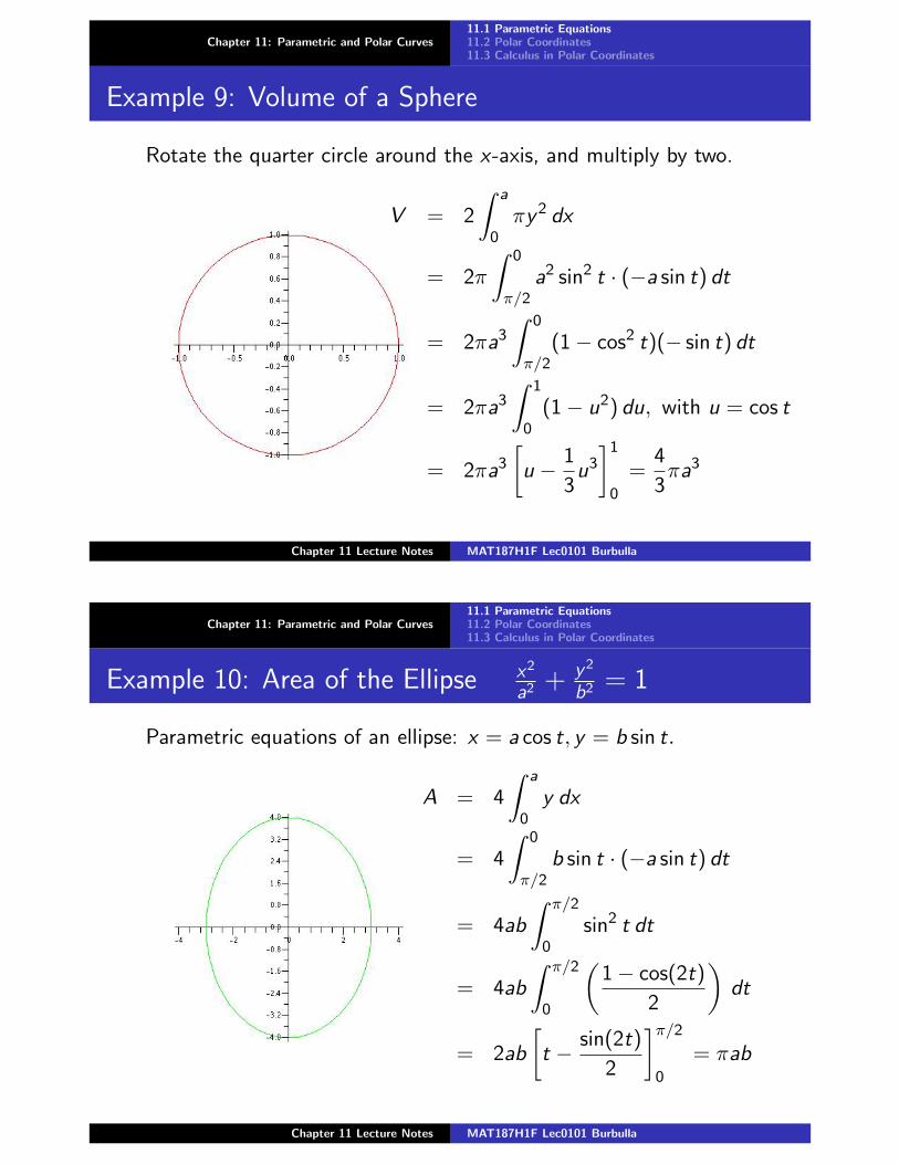
Example 9: Volume of a Sphere

Rotate the quarter circle around the x-axis, and multiply by two.

V = 2

∫ a

0πy2 dx

= 2π

∫ 0

π/2a2 sin2 t · (−a sin t) dt

= 2πa3

∫ 0

π/2(1− cos2 t)(− sin t) dt

= 2πa3

∫ 1

0(1− u2) du, with u = cos t

= 2πa3

[u − 1

3u3

]1

0

=4

3πa3



Example 10: Area of the Ellipse x2

a2 + y2

b2 = 1

Parametric equations of an ellipse: x = a cos t, y = b sin t.

A = 4

∫ a

0y dx

= 4

∫ 0

π/2b sin t · (−a sin t) dt

= 4ab

∫ π/2

0sin2 t dt

= 4ab

∫ π/2

0

(1− cos(2t)

2

)dt

= 2ab

[t − sin(2t)

2

]π/2

0

= πab



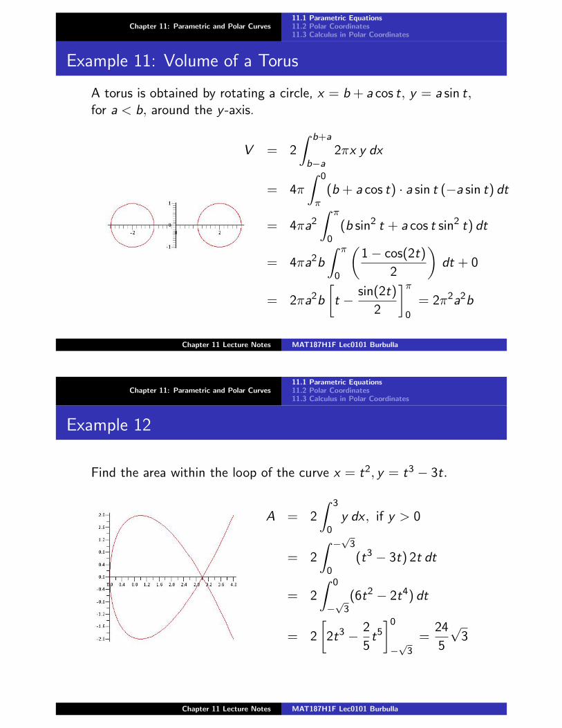
Example 11: Volume of a Torus

A torus is obtained by rotating a circle, x = b + a cos t, y = a sin t,for a < b, around the y -axis.

V = 2

∫ b+a

b−a2πx y dx

= 4π

∫ 0

π(b + a cos t) · a sin t (−a sin t) dt

= 4πa2

∫ π

0(b sin2 t + a cos t sin2 t) dt

= 4πa2b

∫ π

0

(1− cos(2t)

2

)dt + 0

= 2πa2b

[t − sin(2t)

2

]π

0

= 2π2a2b



Example 12

Find the area within the loop of the curve x = t2, y = t3 − 3t.

A = 2

∫ 3

0y dx , if y > 0

= 2

∫ −√

3

0(t3 − 3t) 2t dt

= 2

∫ 0

−√

3(6t2 − 2t4) dt

= 2

[2t3 − 2

5t5

]0

−√

3

=24

5

√3



What Are Polar Coordinates?

x

y

rO

rP(x , y)

��

�r

θ

1. Let the point P haveCartesian coordinates (x , y)

2. Let r be the length of OP.

3. Let θ be the angle the line OPmakes with the positive x-axis.

4. Then r and θ are called thepolar coordinates of P.

We havex = r cos θ and y = r sin θ.

Equivalently,

r =√

x2 + y2 and tan θ =y

x.

The value of θ depends on which quadrant (x , y) is in.



Example 1

Find the polar coordinates of the following points. Warning: polarcoordinates are not unique because θ is not unique.

(x , y) (r , θ) with angles chosen from [−2π, 2π]

(2, 0) r = 2, θ = 0 or θ = 2π

(1, 1) r =√

2, θ = π/4(0, 1) r = 1, θ = π/2

(0,−3) r = 3, θ = −π/2 or θ = 3π/2(−2, 0) r = 2, θ = π or θ = −π

(−1,−√

3) r = 2, θ = 4π/3 or θ = −2π/3(3,−4) r =

√9 + 16 = 5, θ = tan−1

(−4

3

)' −0.927 radians

(0, 0) r = 0, θ can be anything.



Negative Values of r

According to the definition of polar coordinates, r should bepositive. However, we can extend the definition to include negativevalues of r . Suppose r < 0.

x

y

rr

P(−x ,−y)

rQ(x , y)

��

�−r

θO

1. Let Q have coordinates (x , y)and polar coordinates (−r , θ).

2. Then the point P with polarcoordinates (r , θ) is defined to bethe point with polar coordinates(−r , θ ± π).

3. That is,−→OP = −

−→OQ.



Example 2

The point with polar coordinates

(r , θ) =(−3,

π

2

)is the same as the point with polarcoordinates(

3,π

2− π

)=(3,−π

2

).

Its Cartesian coordinates are

(x , y) = (0,−3).

x

y(0, 3)

r

b

(0,−3)

π/2

−π/2



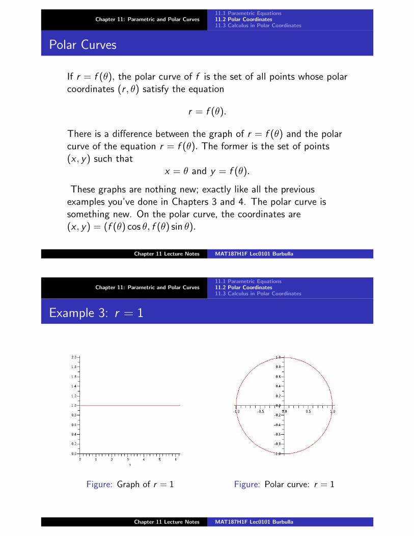
Polar Curves

If r = f (θ), the polar curve of f is the set of all points whose polarcoordinates (r , θ) satisfy the equation

r = f (θ).

There is a difference between the graph of r = f (θ) and the polarcurve of the equation r = f (θ). The former is the set of points(x , y) such that

x = θ and y = f (θ).

These graphs are nothing new; exactly like all the previousexamples you’ve done in Chapters 3 and 4. The polar curve issomething new. On the polar curve, the coordinates are(x , y) = (f (θ) cos θ, f (θ) sin θ).



Example 3: r = 1

Figure: Graph of r = 1 Figure: Polar curve: r = 1



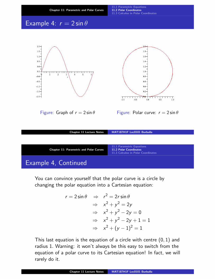
Example 4: r = 2 sin θ

Figure: Graph of r = 2 sin θ Figure: Polar curve: r = 2 sin θ



Example 4, Continued

You can convince yourself that the polar curve is a circle bychanging the polar equation into a Cartesian equation:

r = 2 sin θ ⇒ r2 = 2r sin θ

⇒ x2 + y2 = 2y

⇒ x2 + y2 − 2y = 0

⇒ x2 + y2 − 2y + 1 = 1

⇒ x2 + (y − 1)2 = 1

This last equation is the equation of a circle with centre (0, 1) andradius 1. Warning: it won’t always be this easy to switch from theequation of a polar curve to its Cartesian equation! In fact, we willrarely do it.



Exampl 5: r = 1 + cos θ

Figure: Graph of the functionr = 1 + cos θ

Figure: Cardioid with polarequation: r = 1 + cos θ



Example 6: r = 2 + cos θ

Figure: Graph of the functionr = 2 + cos θ

Figure: Curve with polarequation: r = 2 + cos θ



Example 7: r = 1− 2 cos θ

Figure: Graph of the functionr = 1− 2 cos θ

Figure: Limacon with polarequation: r = 1− 2 cos θ




The limacon has an interesting feature: a loop within a loop. Forwhich angles does the curve of r = 1− 2 cos θ trace out the outerloop? the inner loop? The two loops have only one point incommon, the origin (0, 0), at which r = 0. The boundary angles ofthe loops are found by solving

r = 0⇔ cos θ =1

2⇒ θ =

π

3or

5π

3.

The outer loop, when r > 0, is traced for

π

3< θ <

5π

3.

For −π

3< θ <

π

3, r < 0 and the curve traces out the inner loop.



Example 8: r = 2 sin(2θ)

Figure: Graph of the functionr = 2 sin(2θ)

Figure: Four leaved rose withpolar equation: r = 2 sin(2θ)



Example 9: r = 2 sin(3θ)

Figure: Graph of the functionr = 2 sin(3θ)

Figure: Three leaved rose withpolar equation: r = 2 sin(3θ)



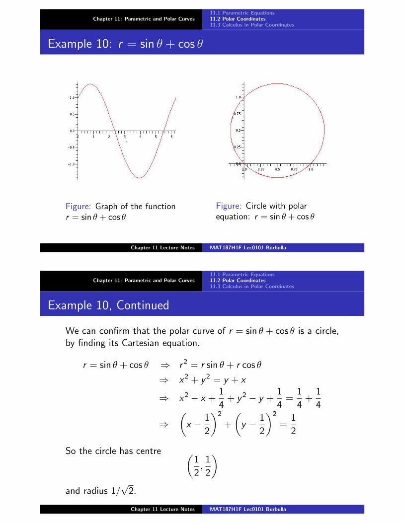
Example 10: r = sin θ + cos θ

Figure: Graph of the functionr = sin θ + cos θ

Figure: Circle with polarequation: r = sin θ + cos θ




We can confirm that the polar curve of r = sin θ + cos θ is a circle,by finding its Cartesian equation.

r = sin θ + cos θ ⇒ r2 = r sin θ + r cos θ

⇒ x2 + y2 = y + x

⇒ x2 − x +1

4+ y2 − y +

1

4=

1

4+

1

4

⇒(

x − 1

2

)2

+

(y − 1

2

)2

=1

2

So the circle has centre (1

2,1

2

)and radius 1/

√2.



Example 11: r = θ/25

Figure: Graph of the functionr = θ/25, θ ≥ 0

Figure: Archimedean spiral withpolar equation: r = θ/25, θ ≥ 0



Example 12: r = eθ/25

Figure: Graph of the functionr = eθ/25

Figure: Logarithmic spiral withpolar equation: r = eθ/25



Derivatives for Polar Curves

Since the parametric equations for a polar curve are

x = r cos θ, y = r sin θ,

the first derivative of a polar curve is

dy

dx=

dy

dθdx

dθ

=sin θ

dr

dθ+ r cos θ

cos θdr

dθ− r sin θ

.

The formula for the second derivative is so messy we won’t eventry to write it down!



Example 1

Find the slope of the tangent line to the circle with polar equationr = 4 cos θ at the point with θ = π/6.

dy

dx=

sin θdr

dθ+ r cos θ

cos θdr

dθ− r sin θ

=−4 sin2 θ + 4 cos2 θ

−4 cos θ sin θ − 4 cos θ sin θ

=sin2 θ − cos2 θ

2 sin θ cos θ= − cot(2θ)

So at θ = π/6 the slope is − cot(π/3) = −1/√

3.



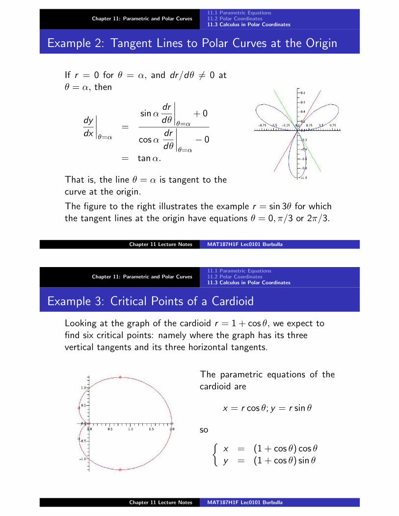
Example 2: Tangent Lines to Polar Curves at the Origin

If r = 0 for θ = α, and dr/dθ 6= 0 atθ = α, then

dy

dx

∣∣∣∣θ=α

=

sin αdr

dθ

∣∣∣∣θ=α

+ 0

cos αdr

dθ

∣∣∣∣θ=α

− 0

= tanα.

That is, the line θ = α is tangent to thecurve at the origin.

The figure to the right illustrates the example r = sin 3θ for whichthe tangent lines at the origin have equations θ = 0, π/3 or 2π/3.



Example 3: Critical Points of a Cardioid

Looking at the graph of the cardioid r = 1 + cos θ, we expect tofind six critical points: namely where the graph has its threevertical tangents and its three horizontal tangents.

The parametric equations of thecardioid are

x = r cos θ; y = r sin θ

so {x = (1 + cos θ) cos θy = (1 + cos θ) sin θ



Horizontal Tangents to the Cardioid r = 1 + cos θ

dy

dθ= 0 ⇔ d

dθ((1 + cos θ) sin θ) = 0

⇔ − sin2 θ + cos θ + cos2 θ = 0

⇔ cos2 θ + cos θ − (1− cos2 θ) = 0

⇔ 2 cos2 θ + cos θ − 1 = 0

⇔ (2 cos θ − 1)(cos θ + 1) = 0

⇔ cos θ =1

2or cos θ = −1

Find the critical points: cos θ = −1⇒ r = 0⇒ (x , y) = (0, 0).

cos θ =1

2⇒ r =

3

2and sin θ = ±

√3

2⇒ (x , y) =

(3

4,±3

√3

4

).



Vertical Tangents to the Cardioid r = 1 + cos θ

dx

dθ= 0 ⇔ d

dθ((1 + cos θ) cos θ) = 0

⇔ − sin θ cos θ − sin θ − sin θ cos θ = 0

⇔ sin θ(1 + 2 cos θ) = 0

⇔ cos θ = −1

2or sin θ = 0

Find the critical points:

cos θ = −1

2⇒ r =

1

2and sin θ = ±

√3

2⇒ (x , y) =

(−1

4,±√

3

4

).

sin θ = 0⇒ cos θ = ±1⇒ r = 0 or 2. Take (x , y) = (2, 0).



Example 4: Logarithmic Spiral r = eθ/25 Revisited

Note: for the following, the algebra is easier if r = eθ, but then thecurve spirals out so quickly that it is hard to get a suitable graph.

The parametric equations of thisspiral are

x = eθ/25 cos θ, y = eθ/25 sin θ;

dy

dx=

1/25eθ/25 sin θ + eθ/25 cos θ

1/25eθ/25 cos θ − eθ/25 sin θ

=sin θ + 25 cos θ

cos θ − 25 sin θ



dy

dx= m ⇔ sin θ + 25 cos θ

cos θ − 25 sin θ= m

⇔ sin θ + 25 cos θ = m(cos θ − 25 sin θ)

⇔ (1 + 25m) sin θ = (m − 25) cos θ

⇔ tan θ =m − 25

1 + 25m

1. m = 0⇒ tan θ = −25. This means that all the points on thespiral with slope zero lineup along the line y = −25x .

2. m = ±∞⇒ tan θ = 125 . This means that all the points on the

spiral with undefined slope lineup along the line y = x/25.

3. m = 1⇒ tan θ = −1213 . This means that all the points on the

spiral with slope 1 lineup along the line y = −1213x .

4. m = −1⇒ tan θ = 1312 . This means that all the points on the

spiral with slope -1 lineup along the line y = 1312x .



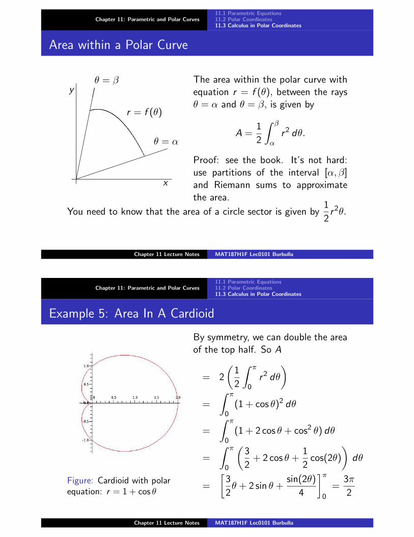
Area within a Polar Curve

x

y

��

θ = β

θ = α

r = f (θ)

��

The area within the polar curve withequation r = f (θ), between the raysθ = α and θ = β, is given by

A =1

2

∫ β

αr2 dθ.

Proof: see the book. It’s not hard:use partitions of the interval [α, β]and Riemann sums to approximatethe area.

You need to know that the area of a circle sector is given by1

2r2θ.



Example 5: Area In A Cardioid

Figure: Cardioid with polarequation: r = 1 + cos θ

By symmetry, we can double the areaof the top half. So A

= 2

(1

2

∫ π

0r2 dθ

)=

∫ π

0(1 + cos θ)2 dθ

=

∫ π

0(1 + 2 cos θ + cos2 θ) dθ

=

∫ π

0

(3

2+ 2 cos θ +

1

2cos(2θ)

)dθ

=

[3

2θ + 2 sin θ +

sin(2θ)

4

]π

0

=3π

2



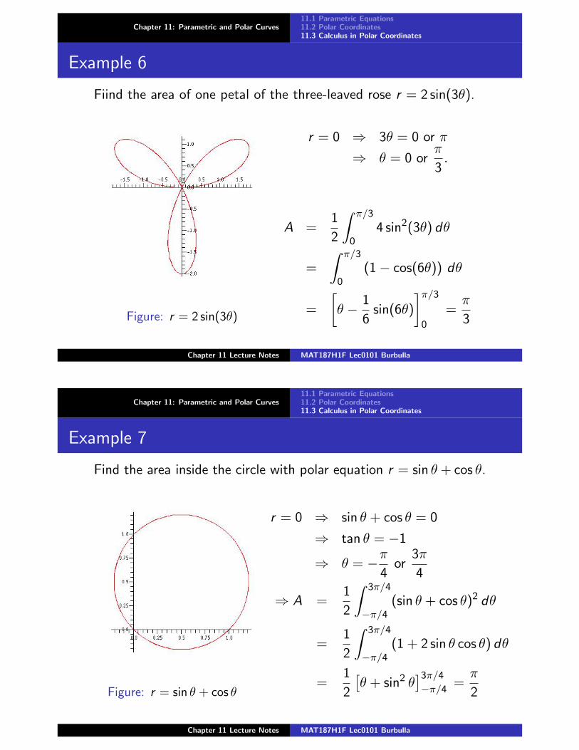
Example 6

Fiind the area of one petal of the three-leaved rose r = 2 sin(3θ).

Figure: r = 2 sin(3θ)

r = 0 ⇒ 3θ = 0 or π

⇒ θ = 0 orπ

3.

A =1

2

∫ π/3

04 sin2(3θ) dθ

=

∫ π/3

0(1− cos(6θ)) dθ

=

[θ − 1

6sin(6θ)

]π/3

0

=π

3



Example 7

Find the area inside the circle with polar equation r = sin θ + cos θ.

Figure: r = sin θ + cos θ

r = 0 ⇒ sin θ + cos θ = 0

⇒ tan θ = −1

⇒ θ = −π

4or

3π

4

⇒ A =1

2

∫ 3π/4

−π/4(sin θ + cos θ)2 dθ

=1

2

∫ 3π/4

−π/4(1 + 2 sin θ cos θ) dθ

=1

2

[θ + sin2 θ

]3π/4

−π/4=

π

2



Example 8

Figure: r = 1− 2 cos θ

Find the area within each ofthe inner and outer loops of thelimacon: Recall, that the outerloop, r > 0, is traced out for

θ ∈ [π/3, 5π/3],

and that inner loop, r < 0, istraced out for

θ ∈ [−π/3, π/3].

Let Ai be the area of the innerloop; let Ao be the area of theouter loop.




A0 = 2

(1

2

∫ π

π/3(1− 2 cos θ)2 dθ

)=

∫ π

π/3(1− 4 cos θ + 4 cos2 θ) dθ

=

∫ π

π/3(3− 4 cos θ + 2 cos(2θ)) dθ = [3θ − 4 sin θ + sin(2θ)]ππ/3

= 3π − 3(π/3) + 4 sin(π/3)− sin(2π/3) = 2π +3

2

√3

Ai = 2

(1

2

∫ π/3

0(1− 2 cos θ)2 dθ

)= [3θ − 4 sin θ + sin(2θ)]

π/30

= 3(π/3)− 4 sin(π/3) + sin(2π/3) = π − 3

2

√3



Area Between Curves

x

y

��

θ = β

θ = α

r1

r2

��

If the two polar curves r1 and r2 in-tersect at θ = α and θ = β, then thearea between the curves is given by

A =1

2

∫ β

α

(r21 − r2

2

)dθ.

This is simply the area within r1 mi-nus the area within r2.



Example 9

Find the area inside the limacon r = 1 + 2 cos θ but outside thecircle r = 2. Have: 1 + 2 cos θ = 2⇒ cos θ = 1/2⇒ θ = ±π/3.

A = 2

(1

2

∫ π/3

0

((1 + 2 cos θ)2 − 22

)dθ

)

=

∫ π/3

0

(−3 + 4 cos θ + 4 cos2 θ

)dθ

=

∫ π/3

0(−1 + 4 cos θ + 2 cos(2θ)) dθ

= [−θ + 4 sin θ + sin(2θ)]π/30

= −π/3 + 4 sin(π/3) + sin(2π/3)

= 5√

3/2− π/3



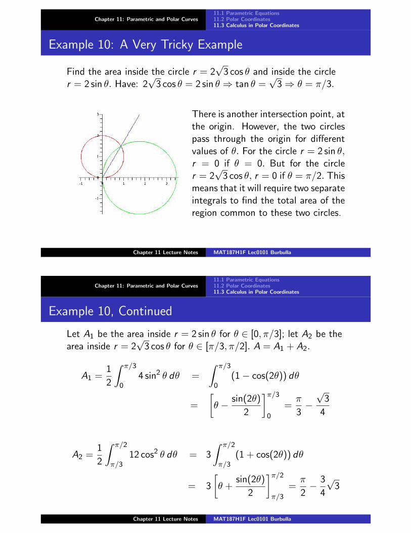
Example 10: A Very Tricky Example

Find the area inside the circle r = 2√

3 cos θ and inside the circler = 2 sin θ. Have: 2

√3 cos θ = 2 sin θ ⇒ tan θ =

√3⇒ θ = π/3.

There is another intersection point, atthe origin. However, the two circlespass through the origin for differentvalues of θ. For the circle r = 2 sin θ,r = 0 if θ = 0. But for the circler = 2

√3 cos θ, r = 0 if θ = π/2. This

means that it will require two separateintegrals to find the total area of theregion common to these two circles.




Let A1 be the area inside r = 2 sin θ for θ ∈ [0, π/3]; let A2 be thearea inside r = 2

√3 cos θ for θ ∈ [π/3, π/2]. A = A1 + A2.

A1 =1

2

∫ π/3

04 sin2 θ dθ =

∫ π/3

0(1− cos(2θ)) dθ

=

[θ − sin(2θ)

2

]π/3

0

=π

3−√

3

4

A2 =1

2

∫ π/2

π/312 cos2 θ dθ = 3

∫ π/2

π/3(1 + cos(2θ)) dθ

= 3

[θ +

sin(2θ)

2

]π/2

π/3

=π

2− 3

4

√3



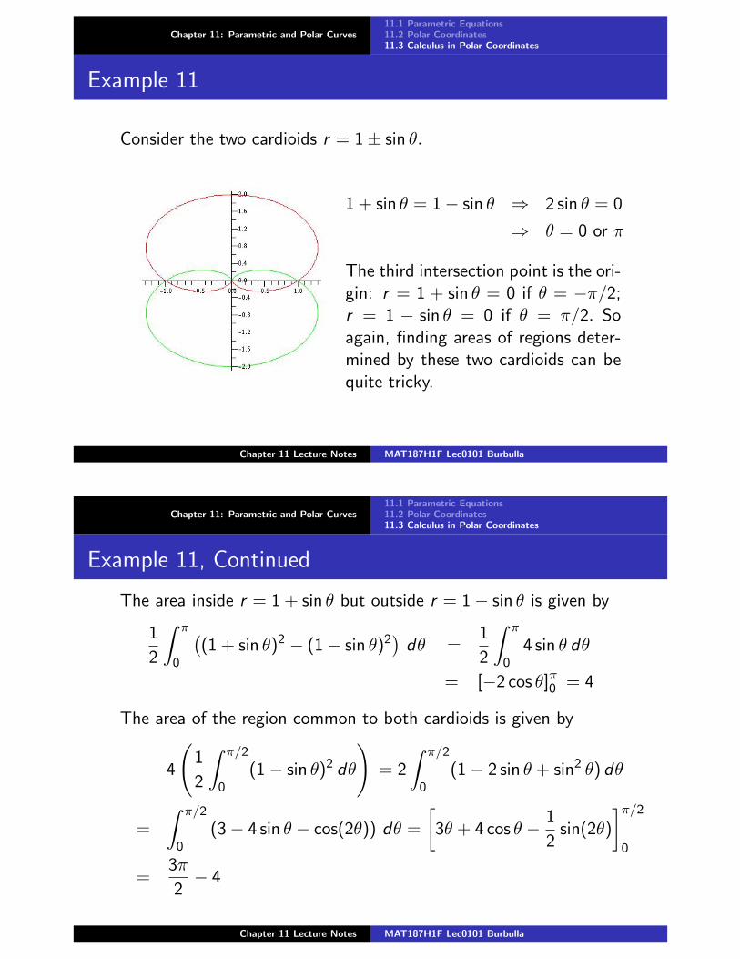
Example 11

Consider the two cardioids r = 1± sin θ.

1 + sin θ = 1− sin θ ⇒ 2 sin θ = 0

⇒ θ = 0 or π

The third intersection point is the ori-gin: r = 1 + sin θ = 0 if θ = −π/2;r = 1 − sin θ = 0 if θ = π/2. Soagain, finding areas of regions deter-mined by these two cardioids can bequite tricky.




The area inside r = 1 + sin θ but outside r = 1− sin θ is given by

1

2

∫ π

0

((1 + sin θ)2 − (1− sin θ)2

)dθ =

1

2

∫ π

04 sin θ dθ

= [−2 cos θ]π0 = 4

The area of the region common to both cardioids is given by

4

(1

2

∫ π/2

0(1− sin θ)2 dθ

)= 2

∫ π/2

0(1− 2 sin θ + sin2 θ) dθ

=

∫ π/2

0(3− 4 sin θ − cos(2θ)) dθ =

[3θ + 4 cos θ − 1

2sin(2θ)

]π/2

0

=3π

2− 4



Example 12: The Problem of Intersection Points

Consider the polar curves r = 1 + sin θ and r2 = 4 sin θ. The polarcurve r2 = 4 sin θ comes in two parts: r = ±2

√sin θ, for θ ∈ [0, π].

From the graphs we expect four in-tersection points. Substituting for rfrom one equation into the other:

(1 + sin θ)2 = 4 sin θ

⇒ 1 + 2 sin θ + sin2 θ = 4 sin θ

⇒ 1− 2 sin θ + sin2 θ = 0

⇒ (1− sin θ)2 = 0

⇒ sin θ = 1

⇒ θ = π/2, at (x , y) = (0, 2).



Example 12: What are the other three intersection points?

(0, 0) is one obvious other intersection point. For r = 1 + sin θ,r = 0 if θ = 3π/2; for r2 = 4 sin θ, r = 0 if θ = 0 or π. But how toget the other two intersection points? Recall that the point withpolar coordinates (r , θ) is the same as the point with polarcoordinates (−r , θ ± π). Rewrite the polar equation r2 = 4 sin θ as

(−r)2 = 4 sin(θ ± π)⇔ r2 = 4(− sin θ) = −4 sin θ,

for −π ≤ θ ≤ 0. Now substitute r = 1 + sin θ :

(1 + sin θ)2 = −4 sin θ ⇒ 1 + 2 sin θ + sin2 θ = −4 sin θ

⇒ sin2 θ + 6 sin θ + 1 = 0

⇒ sin θ = −3± 2√

2⇒ sin θ = −3 + 2√

2

⇒ θ ' −9.879 or − 170.121 in degrees.



Example 12, Concluded

If sin θ = −3 + 2√

2, then

cos θ = ±√

1− (−3 + 2√

2)2 = ±2

√3√

2− 4,

and r = 1 + (−3 + 2√

2) = −2 + 2√

2. The Cartesian coordinatesof the remaining two intersection points are:

(x , y) = (r cos θ, r sin θ)

=

(±4(

√2− 1)

√3√

2− 4, 14− 10√

2

)' (±0.8161427336,−0.14213562)



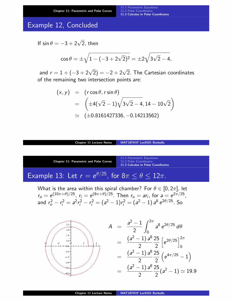
Example 13: Let r = eθ/25, for 8π ≤ θ ≤ 12π.

What is the area within this spiral chamber? For θ ∈ [0, 2π], letro = e(10π+θ)/25, ri = e(8π+θ)/25. Then ro = ari , for a = e2π/25,and r2

o − r2i = a2r2

i − r2i = (a2 − 1)r2

i = (a2 − 1) a8 e2θ/25. So

A =a2 − 1

2

∫ 2π

0a8 e2θ/25 dθ

=(a2 − 1) a8

2

25

2

[e2θ/25

]2π

0

=(a2 − 1) a8

2

25

2

(e4π/25 − 1

)=

(a2 − 1) a8

2

25

2(a2 − 1) ' 19.9


Documents

MAT187H1F Lec0101 Burbulla - math.utoronto.ca · Chapter 11: Parametric and Polar Curves MAT187H1F Lec0101 Burbulla Chapter 11 Lecture Notes Spring 2017 Chapter 11 Lecture Notes MAT187H1F