Embed Size (px)
Citation preview

Delft Center for Systems and Control
A Nonlinear Model PredictiveControl based EvasiveManoeuvre Assist Function
Gijs van Lookeren Campagne
Mas
tero
fScie
nce
Thes
is


A Nonlinear Model Predictive Controlbased Evasive Manoeuvre Assist
Function
Master of Science Thesis
For the degree of Master of Science in Systems and Control at DelftUniversity of Technology
Gijs van Lookeren Campagne
June 21, 2019
Faculty of Mechanical, Maritime and Materials Engineering (3mE) · Delft University ofTechnology

The work in this thesis was supported by Volvo Car Corporation. Their cooperation isgratefully acknowledged.
Copyright c© Delft Center for Systems and Control (DCSC)All rights reserved.
Abstract
In recent years, research in the field of autonomous driving has been subject to a signifi-cant increase in interest. Along with the advances in automation and electrification, carsare slowly transitioning to computers on wheels. The ever-increasing processing power invehicles gives rise to the implementation of advanced control strategies. The increase in com-putational power not only allows for novel solutions to automated driving but can also beused for advanced control systems aimed at collision avoidance. At the same time, significantadvances have been made towards efficient nonlinear optimisation methods, giving rise to newpossibilities for real-time applications.
This thesis focuses on an Evasive Manoeuvre Assistance Function (EMA) to avoid obstaclesat the limits of handling using a Model Predictive Control (MPC) approach. Vehicles atthe limits of handling typically operate in the nonlinear region of the tyre. For this reason,a Nonlinear Model Predictive Control (NMPC) approach is employed. A baseline scenariowith a lateral displacement of 2 metres is considered, representing a common near rear-endcollision situation. An optimal trajectory and steering sequence is computed by the MPCover a defined horizon. As MPC considers a model to calculate an optimal control input, anonlinear two-track model with a simplified Magic Formula is used.
The main drawback of real-time NMPC has always been its computational burden. For thebaseline scenario, the limits of real-time NMPC are explored, using the state-of-the-art non-linear optimisation methods: Sequential Quadratic Programming (SQP) and Interior-PointMethod (IPM). Both methods are compared in simulation and an SQP approach is tested onan embedded system within a test vehicle, subject to the disturbances and uncertainties thatcome with physical driving.
It was found that the proposed NMPC strategies make for a robust yet aggressive manoeuvrewith high lateral accelerations, utilising the nonlinear operating region of the tyre. Further-more, computation times on an embedded system in a test vehicle were found to be sufficientlylow for real-time application.
Master of Science Thesis Gijs van Lookeren Campagne

ii
Gijs van Lookeren Campagne Master of Science Thesis
Table of Contents
Preface xiii
1 Introduction 11-1 Motivation . . . . . . . . . . . . . . . . . . . . . . . . . . . . . . . . . . . . . . 11-2 Problem definition . . . . . . . . . . . . . . . . . . . . . . . . . . . . . . . . . . 31-3 Major contributions . . . . . . . . . . . . . . . . . . . . . . . . . . . . . . . . . 51-4 Thesis outline . . . . . . . . . . . . . . . . . . . . . . . . . . . . . . . . . . . . 5
2 Literature survey 72-1 Current state-of-the-art . . . . . . . . . . . . . . . . . . . . . . . . . . . . . . . 72-2 Design choices . . . . . . . . . . . . . . . . . . . . . . . . . . . . . . . . . . . . 8
3 System dynamics 113-1 Vehicle coordinate frames . . . . . . . . . . . . . . . . . . . . . . . . . . . . . . 123-2 Vehicle model . . . . . . . . . . . . . . . . . . . . . . . . . . . . . . . . . . . . 12
3-2-1 Vehicle model for steering only scenario . . . . . . . . . . . . . . . . . . 133-2-2 Vehicle model for steering and braking scenario . . . . . . . . . . . . . . 14
3-3 Nonlinear tyre model . . . . . . . . . . . . . . . . . . . . . . . . . . . . . . . . 15
4 Model Predictive Control 174-1 What is MPC? . . . . . . . . . . . . . . . . . . . . . . . . . . . . . . . . . . . . 174-2 Motivation for MPC . . . . . . . . . . . . . . . . . . . . . . . . . . . . . . . . . 194-3 Solving the MPC problem . . . . . . . . . . . . . . . . . . . . . . . . . . . . . . 204-4 Constraints . . . . . . . . . . . . . . . . . . . . . . . . . . . . . . . . . . . . . . 204-5 Implementation . . . . . . . . . . . . . . . . . . . . . . . . . . . . . . . . . . . 21
Master of Science Thesis Gijs van Lookeren Campagne
iv Table of Contents
5 Nonlinear programming 235-1 Transcription methods . . . . . . . . . . . . . . . . . . . . . . . . . . . . . . . . 24
5-1-1 Multiple Shooting method . . . . . . . . . . . . . . . . . . . . . . . . . 255-1-2 Direct collocation method . . . . . . . . . . . . . . . . . . . . . . . . . . 27
5-2 Sequential Quadratic Programming . . . . . . . . . . . . . . . . . . . . . . . . . 295-3 Interior-point Method . . . . . . . . . . . . . . . . . . . . . . . . . . . . . . . . 33
6 Simulation results 356-1 Interior-Point Method (IPM) . . . . . . . . . . . . . . . . . . . . . . . . . . . . 38
6-1-1 Steering only (IPM) formulation . . . . . . . . . . . . . . . . . . . . . . 386-1-2 Steering & braking (IPM) formulation . . . . . . . . . . . . . . . . . . . 396-1-3 Trajectory (IPM) . . . . . . . . . . . . . . . . . . . . . . . . . . . . . . 406-1-4 Notable results (IPM) . . . . . . . . . . . . . . . . . . . . . . . . . . . . 41
6-2 Sequential Quadratic Programming (SQP) . . . . . . . . . . . . . . . . . . . . . 436-2-1 Steering only (SQP) formulation . . . . . . . . . . . . . . . . . . . . . . 436-2-2 Trajectory (SQP) . . . . . . . . . . . . . . . . . . . . . . . . . . . . . . 446-2-3 Notable results (SQP) . . . . . . . . . . . . . . . . . . . . . . . . . . . . 44
6-3 Overview of simulation results . . . . . . . . . . . . . . . . . . . . . . . . . . . 45
7 Experimental results 477-1 Experimental setup . . . . . . . . . . . . . . . . . . . . . . . . . . . . . . . . . 477-2 Obtaining the measurement states . . . . . . . . . . . . . . . . . . . . . . . . . 507-3 Torque request . . . . . . . . . . . . . . . . . . . . . . . . . . . . . . . . . . . . 507-4 Results . . . . . . . . . . . . . . . . . . . . . . . . . . . . . . . . . . . . . . . . 52
7-4-1 Trajectory . . . . . . . . . . . . . . . . . . . . . . . . . . . . . . . . . . 537-4-2 Notable results . . . . . . . . . . . . . . . . . . . . . . . . . . . . . . . 54
7-5 Friction utilisation . . . . . . . . . . . . . . . . . . . . . . . . . . . . . . . . . . 557-6 Overview of results . . . . . . . . . . . . . . . . . . . . . . . . . . . . . . . . . 56
8 Conclusion 578-1 Recommendations . . . . . . . . . . . . . . . . . . . . . . . . . . . . . . . . . . 58
8-1-1 Stability constraints . . . . . . . . . . . . . . . . . . . . . . . . . . . . . 588-1-2 More advanced vehicle model . . . . . . . . . . . . . . . . . . . . . . . . 588-1-3 Implementation with additional driver applied torque . . . . . . . . . . . 598-1-4 Longitudinal inputs on an experimental setup . . . . . . . . . . . . . . . 598-1-5 Obstacle dependent cost function for collision avoidance . . . . . . . . . 598-1-6 Experimental tests with higher steering wheel torque limits . . . . . . . . 598-1-7 Embedded implementation of IPM . . . . . . . . . . . . . . . . . . . . . 598-1-8 Spatial formulation for MPC . . . . . . . . . . . . . . . . . . . . . . . . 60
Gijs van Lookeren Campagne Master of Science Thesis

Table of Contents v
A Simulation results 61A-1 SQP & IPM (steering only) compared at computational limits . . . . . . . . . . 61
A-1-1 SQP & IPM (steering only) formulation . . . . . . . . . . . . . . . . . . 61A-1-2 Trajectory . . . . . . . . . . . . . . . . . . . . . . . . . . . . . . . . . . 62A-1-3 Notable results . . . . . . . . . . . . . . . . . . . . . . . . . . . . . . . 63A-1-4 Computation times . . . . . . . . . . . . . . . . . . . . . . . . . . . . . 64A-1-5 Friction utilisation . . . . . . . . . . . . . . . . . . . . . . . . . . . . . . 65
A-2 IPM (steering only) . . . . . . . . . . . . . . . . . . . . . . . . . . . . . . . . . 69A-2-1 Trajectory . . . . . . . . . . . . . . . . . . . . . . . . . . . . . . . . . . 69A-2-2 Notable results . . . . . . . . . . . . . . . . . . . . . . . . . . . . . . . 70A-2-3 Computation times . . . . . . . . . . . . . . . . . . . . . . . . . . . . . 70A-2-4 Friction utilisation . . . . . . . . . . . . . . . . . . . . . . . . . . . . . . 70
A-3 IPM (Steering & braking) . . . . . . . . . . . . . . . . . . . . . . . . . . . . . . 72A-3-1 Computation times . . . . . . . . . . . . . . . . . . . . . . . . . . . . . 72A-3-2 Friction utilisation . . . . . . . . . . . . . . . . . . . . . . . . . . . . . . 73
A-4 SQP (steering only) . . . . . . . . . . . . . . . . . . . . . . . . . . . . . . . . . 74A-4-1 Computation times . . . . . . . . . . . . . . . . . . . . . . . . . . . . . 74A-4-2 Friction utilisation . . . . . . . . . . . . . . . . . . . . . . . . . . . . . . 75
A-5 Scalability to different scenarios . . . . . . . . . . . . . . . . . . . . . . . . . . . 76A-5-1 Comparison of multiple references . . . . . . . . . . . . . . . . . . . . . 76A-5-2 Comparison of multiple initial velocities . . . . . . . . . . . . . . . . . . 78
A-6 Horizon comparison . . . . . . . . . . . . . . . . . . . . . . . . . . . . . . . . . 79A-6-1 IPM . . . . . . . . . . . . . . . . . . . . . . . . . . . . . . . . . . . . . 79A-6-2 SQP . . . . . . . . . . . . . . . . . . . . . . . . . . . . . . . . . . . . . 79
A-7 Sampling time comparison . . . . . . . . . . . . . . . . . . . . . . . . . . . . . 80A-7-1 IPM . . . . . . . . . . . . . . . . . . . . . . . . . . . . . . . . . . . . . 80A-7-2 SQP . . . . . . . . . . . . . . . . . . . . . . . . . . . . . . . . . . . . . 81
B Experimental results 83B-1 Results at 50 KPH . . . . . . . . . . . . . . . . . . . . . . . . . . . . . . . . . . 83B-2 Results at 60 KPH . . . . . . . . . . . . . . . . . . . . . . . . . . . . . . . . . . 85B-3 Results at 90 KPH . . . . . . . . . . . . . . . . . . . . . . . . . . . . . . . . . . 87B-4 Comparison between driver, simulation and experiment . . . . . . . . . . . . . . 90
Bibliography 91
Glossary 95List of Acronyms . . . . . . . . . . . . . . . . . . . . . . . . . . . . . . . . . . . 95List of Symbols . . . . . . . . . . . . . . . . . . . . . . . . . . . . . . . . . . . 95
Master of Science Thesis Gijs van Lookeren Campagne

vi Table of Contents
Gijs van Lookeren Campagne Master of Science Thesis

List of Figures
1-1 Braking and steering distance compared [1] . . . . . . . . . . . . . . . . . . . . 11-2 Evasive manoeuvre trajectory . . . . . . . . . . . . . . . . . . . . . . . . . . . . 21-3 Friction circle for different kinds of driving behaviour [2] . . . . . . . . . . . . . 31-4 Reference displacement . . . . . . . . . . . . . . . . . . . . . . . . . . . . . . . 41-5 Baseline scenario . . . . . . . . . . . . . . . . . . . . . . . . . . . . . . . . . . . 4
2-1 Overview of literature study outcome . . . . . . . . . . . . . . . . . . . . . . . . 8
3-1 Comparison between nonlinear and linear tyre model . . . . . . . . . . . . . . . 113-2 Vehicle coordinate frames . . . . . . . . . . . . . . . . . . . . . . . . . . . . . . 123-3 Longitudinal wheel dynamics . . . . . . . . . . . . . . . . . . . . . . . . . . . . 143-4 Slip angle . . . . . . . . . . . . . . . . . . . . . . . . . . . . . . . . . . . . . . 153-5 Pacejka’s Magic formula . . . . . . . . . . . . . . . . . . . . . . . . . . . . . . 16
4-1 MPC reference tracking [3] . . . . . . . . . . . . . . . . . . . . . . . . . . . . . 174-2 MPC structure . . . . . . . . . . . . . . . . . . . . . . . . . . . . . . . . . . . . 214-3 Sampling times within MPC . . . . . . . . . . . . . . . . . . . . . . . . . . . . 224-4 Schematic overview of simulation and experimental setup . . . . . . . . . . . . . 22
5-1 Multiple shooting method . . . . . . . . . . . . . . . . . . . . . . . . . . . . . . 255-2 Fourth order Runge-Kutta method . . . . . . . . . . . . . . . . . . . . . . . . . 265-3 Direct collocation method for one control interval . . . . . . . . . . . . . . . . . 275-4 Optimal solution . . . . . . . . . . . . . . . . . . . . . . . . . . . . . . . . . . . 31
6-1 Volvo XC60 in CarMaker . . . . . . . . . . . . . . . . . . . . . . . . . . . . . . 356-2 Trajectory layout . . . . . . . . . . . . . . . . . . . . . . . . . . . . . . . . . . . 376-3 Steering & braking trajectory using IPM . . . . . . . . . . . . . . . . . . . . . . 40
Master of Science Thesis Gijs van Lookeren Campagne

viii List of Figures
6-4 Results of steering & braking scenario using IPM . . . . . . . . . . . . . . . . . 416-5 Brake torques at the front wheels . . . . . . . . . . . . . . . . . . . . . . . . . . 426-6 Trajectory of steering only scenario using SQP . . . . . . . . . . . . . . . . . . . 446-7 Results of steering only scenario using SQP . . . . . . . . . . . . . . . . . . . . 45
7-1 Volvo V40 test vehicle . . . . . . . . . . . . . . . . . . . . . . . . . . . . . . . . 477-2 Code generation procedure . . . . . . . . . . . . . . . . . . . . . . . . . . . . . 487-3 Steering wheel torque model . . . . . . . . . . . . . . . . . . . . . . . . . . . . 517-4 Trajectory of experimental test at vx0 = 70km/h . . . . . . . . . . . . . . . . . 537-5 Requested torque and steering wheel angle at vx0 = 70km/h . . . . . . . . . . . 537-6 Results of experimental test at vx0 = 70km/h . . . . . . . . . . . . . . . . . . . 547-7 Lateral tyre forces and slip angles at vx0 = 70km/h . . . . . . . . . . . . . . . . 55
8-1 Nonlinear phase portrait . . . . . . . . . . . . . . . . . . . . . . . . . . . . . . . 588-2 Influence of formulation type on cost for combined steering & braking . . . . . . 60
A-1 Comparison of trajectories of steering only scenario for SQP and IPM . . . . . . 62A-2 Comparison of results for SQP and IPM . . . . . . . . . . . . . . . . . . . . . . 63A-3 Computation times for SQP and IPM . . . . . . . . . . . . . . . . . . . . . . . 64A-4 Friction utilisation of rear left wheel for SQP and IPM . . . . . . . . . . . . . . 65A-5 Obtained slip angles for SQP and IPM . . . . . . . . . . . . . . . . . . . . . . . 66A-6 Lateral tyre forces and slip angles for SQP . . . . . . . . . . . . . . . . . . . . . 67A-7 Lateral tyre forces and slip angles for IPM . . . . . . . . . . . . . . . . . . . . . 68A-8 Trajectory of steering only scenario using IPM . . . . . . . . . . . . . . . . . . . 69A-9 Results of steering only scenario using IPM . . . . . . . . . . . . . . . . . . . . 70A-10 Computation time of steering only scenario using IPM . . . . . . . . . . . . . . . 71A-11 Utilised friction for steering only scenario using IPM . . . . . . . . . . . . . . . . 71A-12 Brake torques at the rear wheels . . . . . . . . . . . . . . . . . . . . . . . . . . 72A-13 Computation time of steering & braking scenario using IPM . . . . . . . . . . . 72A-14 Utilised friction for steering & braking scenario using IPM . . . . . . . . . . . . . 73A-15 Computation time of steering scenario using SQP . . . . . . . . . . . . . . . . . 74A-16 Utilised friction for steering only scenario using SQP . . . . . . . . . . . . . . . . 75A-17 Scalability of reference position using SQP (N = 40) . . . . . . . . . . . . . . . 76A-18 Scalability of reference position using SQP (N = 80) . . . . . . . . . . . . . . . 77A-19 Scalability of reference position using IPM . . . . . . . . . . . . . . . . . . . . . 77A-20 Scalability of initial velocity using IPM . . . . . . . . . . . . . . . . . . . . . . . 78A-21 Scalability of initial velocity using SQP . . . . . . . . . . . . . . . . . . . . . . . 78A-22 Comparison of different horizons using IPM . . . . . . . . . . . . . . . . . . . . 79A-23 Comparison of different horizons using SQP . . . . . . . . . . . . . . . . . . . . 79A-24 Comparison of different sampling times using IPM . . . . . . . . . . . . . . . . . 80
Gijs van Lookeren Campagne Master of Science Thesis
List of Figures ix
A-25 Comparison of different sampling times using SQP . . . . . . . . . . . . . . . . 81
B-1 Trajectory of experimental test at vx0 = 50km/h . . . . . . . . . . . . . . . . . 84B-2 Results of experimental test at vx0 = 50km/h . . . . . . . . . . . . . . . . . . . 84B-3 Requested torque and steering wheel angle at vx0 = 50km/h . . . . . . . . . . . 85B-4 Trajectory of experimental test at vx0 = 60km/h . . . . . . . . . . . . . . . . . 86B-5 Results of experimental test at vx0 = 60km/h . . . . . . . . . . . . . . . . . . . 86B-6 Requested torque and steering wheel angle at vx0 = 60km/h . . . . . . . . . . . 87B-7 Trajectory of experimental test at vx0 = 90km/h . . . . . . . . . . . . . . . . . 88B-8 Results of experimental test at vx0 = 90km/h . . . . . . . . . . . . . . . . . . . 88B-9 Requested torque and steering wheel angle at vx0 = 90km/h . . . . . . . . . . . 89B-10 Trajectory comparison for driver, simulation and experiment . . . . . . . . . . . 90B-11 Torque request and steering angle comparison for driver, simulation and experiment 90
Master of Science Thesis Gijs van Lookeren Campagne

x List of Figures
Gijs van Lookeren Campagne Master of Science Thesis
List of Tables
1-1 Scenario targets . . . . . . . . . . . . . . . . . . . . . . . . . . . . . . . . . . . 4
4-1 Overview of control methods for collision avoidance manoeuvres [4] . . . . . . . 20
5-1 Overview of approaches for solving the Nonlinear Programme (NLP) . . . . . . . 24
6-1 XC60 vehicle parameters . . . . . . . . . . . . . . . . . . . . . . . . . . . . . . 356-2 Magic Formula tyre parameters . . . . . . . . . . . . . . . . . . . . . . . . . . . 366-3 MPC parameters . . . . . . . . . . . . . . . . . . . . . . . . . . . . . . . . . . . 386-4 Longitudinal wheel parameters . . . . . . . . . . . . . . . . . . . . . . . . . . . 396-5 MPC parameters . . . . . . . . . . . . . . . . . . . . . . . . . . . . . . . . . . . 436-6 Overview of CasADi vs. Acado . . . . . . . . . . . . . . . . . . . . . . . . . . . 466-7 Overview of different tunings in simulation . . . . . . . . . . . . . . . . . . . . . 46
7-1 V40 vehicle parameters . . . . . . . . . . . . . . . . . . . . . . . . . . . . . . . 477-2 Torque model parameters at vx0 = 70km/h . . . . . . . . . . . . . . . . . . . . 527-3 MPC time parameters for experimental setup . . . . . . . . . . . . . . . . . . . 527-4 Overview of all experimental results . . . . . . . . . . . . . . . . . . . . . . . . 56
A-1 MPC parameters . . . . . . . . . . . . . . . . . . . . . . . . . . . . . . . . . . . 62
B-1 Torque model parameters at vx0 = 50km/h . . . . . . . . . . . . . . . . . . . . 83B-2 Experimental results at vx0 = 50km/h . . . . . . . . . . . . . . . . . . . . . . . 83B-3 Torque model parameters at vx0 = 60km/h . . . . . . . . . . . . . . . . . . . . 85B-4 Experimental results at vx0 = 60km/h . . . . . . . . . . . . . . . . . . . . . . . 85B-5 Torque model parameters at vx0 = 90km/h . . . . . . . . . . . . . . . . . . . . 87B-6 Experimental results at vx0 = 90km/h . . . . . . . . . . . . . . . . . . . . . . . 87
Master of Science Thesis Gijs van Lookeren Campagne

xii List of Tables
Gijs van Lookeren Campagne Master of Science Thesis
Preface
MPC is a control strategy that found its origin in the 1970s in the process industry. Known asa computationally expensive control method, it was mainly used for slow processes. In recentyears, due to advances in computing power and efficient novel solvers, MPC has become amore popular solution for applications with shorter sampling times. One of the novel fieldssubject to ongoing experiments with MPC, is the automotive industry.
In March 2019, a Tesla Model 3 crashed into a truck, with autopilot enabled. The roofseparated from the car and the driver was killed during the accident. The circumstances ofthis crash are similar to another fatal autopilot crash, in 2016. In both scenarios, a truckcrossed the Tesla’s path. Travelling at 110 km/h, the vehicle failed to execute an evasivemanoeuvre, as stated by the National Transportation Safety Board (NTSB).
Volvo’s CEO, Håkan Samuelsson, stated that in order to launch autonomous driving suc-cessfully, an enormous amount of computational power is needed. Volvo aims at having alevel 4 autonomous vehicle on the road by 2021, according to the SAE (Society of Automo-tive Engineers) autonomous driving guideline. At level 4, no driver intervention is needed toensure safety. Volvo has also put out its so-called Vision 2020 statement in which it statesthat no one is to be seriously injured or killed by 2020. To achieve this, various AdvancedDriver Assistance Systems (ADAS) systems are put in place so that the vehicle is able toavoid accidents by intervening in emergency scenarios.
In October 2018 the partnership between computer hardware manufacturer NVIDIA andVolvo came about with plans to work together on solutions to autonomous driving. Totake autonomous driving to the next level, powerful integrated computers need to developed.This powerful processing power opens doors not only to novel image processing solutions forautonomous driving, but also to more advanced control strategies to control the car. Theseadvanced control strategies can then be used to create or improve existing ADAS.
This thesis endeavours to use the newly available processing power for efficient advancedcontrol strategies for an emergency manoeuvre, at the limits of handling. The thesis workwas carried out in the Vehicle Motion & Control department at Volvo Cars, Gothenburg. Iwould like to thank my supervisor at Volvo, Derong Yang and my supervisor in Delft, ManuelMazo Espinosa for their assistance during this thesis.
Master of Science Thesis Gijs van Lookeren Campagne

xiv Preface
Gijs van Lookeren Campagne Master of Science Thesis
Chapter 1
Introduction
1-1 Motivation
In 94% of all vehicle crashes the critical pre-event that led to the crash was caused by the driverof the vehicle [5]. The critical reason is often due to a recognition, decision or performanceerror of the driver. In [6] a driving simulator test was carried out for a near collision situation.It was found that in 50% of the accidents a swerving manoeuvre should have been initiated.In most cases however, the driver resorted to braking only. Today’s driver assistance systemsare able to assist drivers through warning signals or braking assistance. For scenarios wheresolely braking is not sufficient, there are currently no assistance systems in place that allowfor complete collision avoidance.
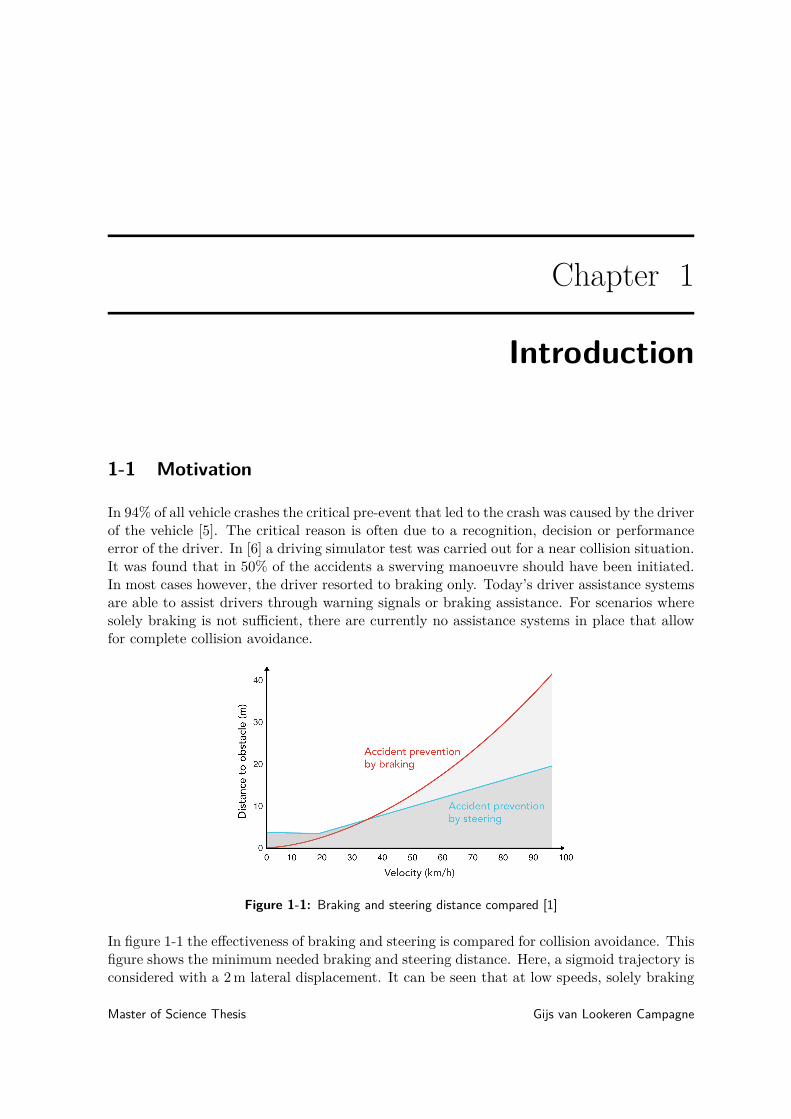
Figure 1-1: Braking and steering distance compared [1]
In figure 1-1 the effectiveness of braking and steering is compared for collision avoidance. Thisfigure shows the minimum needed braking and steering distance. Here, a sigmoid trajectory isconsidered with a 2 m lateral displacement. It can be seen that at low speeds, solely braking
Master of Science Thesis Gijs van Lookeren Campagne
2 Introduction
is sufficient and is in fact a better way to prevent an accident than steering. At higher speeds,the minimum needed distance to avoid the obstacle is lower than for braking. This goes toshow that there is a lot to gain when collision avoidance problems are not only consideredfrom a longitudinal (braking) perspective, but also from a lateral (steering) perspective.
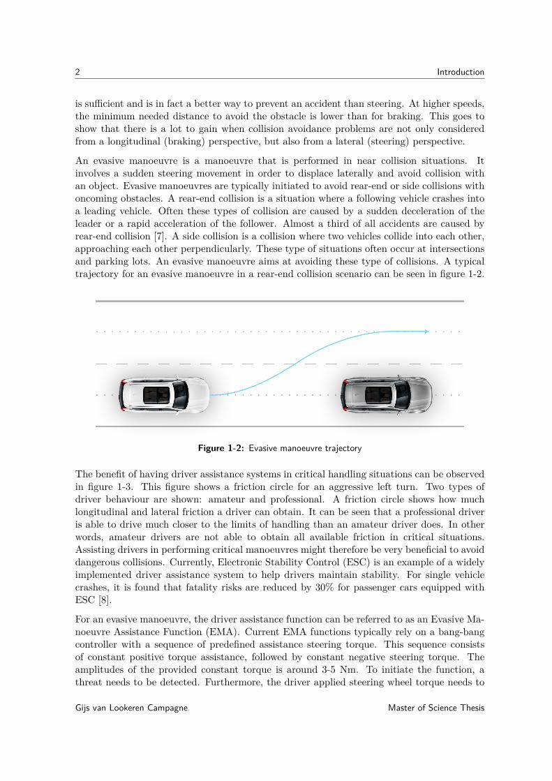
An evasive manoeuvre is a manoeuvre that is performed in near collision situations. Itinvolves a sudden steering movement in order to displace laterally and avoid collision withan object. Evasive manoeuvres are typically initiated to avoid rear-end or side collisions withoncoming obstacles. A rear-end collision is a situation where a following vehicle crashes intoa leading vehicle. Often these types of collision are caused by a sudden deceleration of theleader or a rapid acceleration of the follower. Almost a third of all accidents are caused byrear-end collision [7]. A side collision is a collision where two vehicles collide into each other,approaching each other perpendicularly. These type of situations often occur at intersectionsand parking lots. An evasive manoeuvre aims at avoiding these type of collisions. A typicaltrajectory for an evasive manoeuvre in a rear-end collision scenario can be seen in figure 1-2.
Figure 1-2: Evasive manoeuvre trajectory
The benefit of having driver assistance systems in critical handling situations can be observedin figure 1-3. This figure shows a friction circle for an aggressive left turn. Two types ofdriver behaviour are shown: amateur and professional. A friction circle shows how muchlongitudinal and lateral friction a driver can obtain. It can be seen that a professional driveris able to drive much closer to the limits of handling than an amateur driver does. In otherwords, amateur drivers are not able to obtain all available friction in critical situations.Assisting drivers in performing critical manoeuvres might therefore be very beneficial to avoiddangerous collisions. Currently, Electronic Stability Control (ESC) is an example of a widelyimplemented driver assistance system to help drivers maintain stability. For single vehiclecrashes, it is found that fatality risks are reduced by 30% for passenger cars equipped withESC [8].
For an evasive manoeuvre, the driver assistance function can be referred to as an Evasive Ma-noeuvre Assistance Function (EMA). Current EMA functions typically rely on a bang-bangcontroller with a sequence of predefined assistance steering torque. This sequence consistsof constant positive torque assistance, followed by constant negative steering torque. Theamplitudes of the provided constant torque is around 3-5 Nm. To initiate the function, athreat needs to be detected. Furthermore, the driver applied steering wheel torque needs to
Gijs van Lookeren Campagne Master of Science Thesis

1-2 Problem definition 3
be above a certain threshold value.
Figure 1-3: Friction circle for different kinds of driving behaviour [2]
In order to provide a driver assistance system, a control system needs to be put in place.In this thesis, the application of Model Predictive Control (MPC) is researched to solve theevasive manoeuvre problem. In recent years MPC control strategies have seen a significant in-crease in usage for numerous new applications, among which the automotive industry [9]. Therecent spike in interest to use MPC for new applications can be ascribed to the ever increas-ing processing power in modern day computers. This allows to solve complex optimisationproblems, that were not deemed to be solvable before.
1-2 Problem definition
Rear-end crashes between two vehicle are the type of crashes that occur most frequently[7]. As can be seen in figure 1-4, the obstacle width denotes the lateral displacement neededto avoid the obstacle. It is assumed that using today’s sensor fusion methods, the obstacle’swidth can be measured. This obstacle width serves to create the reference displacement whichis used as an input to the MPC. On average, cars are around 2 m wide [10]. In order to beable to compare different methods and controllers for the same scenario, a baseline obstaclewidth of 2 m is considered throughout this thesis.
The evasive manoeuvre scenario can therefore be described as reaching a lateral referenceposition of 2 m as fast as possible, with a minimal longitudinal displacement Xs, as shown infigure 1-5. In practice, this means that the function needs to be triggered by a set of triggeringconditions. The function then executes a manoeuvre based on the obstacle’s width.
In evasive manoeuvres, cars typically tend to be near the limits of handling. This meansthat the tyres operate near their friction limits. In these conditions, the relation between thelateral tyre forces and the slip of the tyre, is nonlinear. Furthermore, the vehicle dynamics
Master of Science Thesis Gijs van Lookeren Campagne

4 Introduction
Figure 1-4: Reference displacement
are inherently nonlinear. To cope with these nonlinearities, a Nonlinear Model PredictiveControl (NMPC) strategy is considered in this thesis.
In this thesis, the EMA problem will be approached from a fully autonomous perspective. Inother words, no driver applied steering wheel torque is taken into consideration.
Figure 1-5: Baseline scenario
The objective of this thesis is:
To develop a real-time NMPC strategy to laterally displace 2 m within theshortest possible longitudinal displacement.
Based on the literature study, a set of scenario targets is formulated:
Table 1-1: Scenario targets
Scenario target ValueSampling frequency 25 HzLateral acceleration 6-9 m/s2
Longitudinal distance travelled 20-25 mMaximum allowable overshoot 0.5 m
Gijs van Lookeren Campagne Master of Science Thesis

1-3 Major contributions 5
The main novelty of this master thesis is the focus on solving the NMPC problem online. Byregarding state-of-the art solvers, the limits of real-time NMPC are explored. It is assessedwhether this approach is feasible in terms of computational burden. The designed MPC is thentested in the virtual test environment CarMaker before being tested on a rapid prototypingdSPACE system within a physical vehicle.
1-3 Major contributions
This thesis aims to include the following major contributions to the field:
• Analysis of the current possibilities of NMPC for limit handling scenarios, with a focuson dealing with computational complexity.
• Development and testing of a real-time NMPC control strategy on an embedded systemwithin a physical car.
• Comparison of the two major Nonlinear Programme (NLP) solvers for NMPC.
1-4 Thesis outline
In chapter 2, a summary is presented of the literature survey carried out prior to this thesis.Here, emphasis is put on the current state-of-the-art researches in the field and a decisiontree is shown to define the main approach of this thesis. MPC relies on a model of the systemdynamics to define a control input. The nonlinear vehicle and tyre model used in the MPCare discussed in chapter 3. After having defined the model within the MPC, an introductionto MPC is given in chapter 4. In this chapter, the general formulation for MPC is explainedand it advantages over other control strategies are discussed. To solve a nonlinear MPCproblem, NLP methods need to be regarded. The two most renowned methods for solvingnonlinear MPC problems are explained in chapter 5. In chapter 6 and 7 the results of theCarMaker simulation and experimental test runs are discussed, respectively. Finally, basedon the findings in this thesis, a conclusion will be drawn in chapter 8.
Master of Science Thesis Gijs van Lookeren Campagne

6 Introduction
Gijs van Lookeren Campagne Master of Science Thesis

Chapter 2
Literature survey
2-1 Current state-of-the-art
Previous research for limit handling [11] [12] and obstacle avoidance scenarios [13] [4] [14][15] [16] [17] [18] [19] relied on linearisation of the vehicle dynamics in order to cope withthe computional burden. In [20] only the tyre model was linearised. In these researches,in one way or another, concessions were made in terms of model accuracy. A NonlinearModel Predictive Control (NMPC) approach was employed in [21]. For an obstacle avoidancescenario in icy conditions, an obstacle was avoided successfully at vx = 10 m/s, with lowcomputation times. In this research, the proposed Model Predictive Control (MPC) schemewas only tested in simulations.
Experimental tests introduce a novelty to this thesis as there have been few experimentaltests in past research for NMPC based evasive manoeuvre type scenarios. Most researchinvolves simulation only. The additional uncertainties that come with experimental tests(e.g. inaccurate measurement signals) introduce yet another degree of complexity.
There has been some research using NMPC for similar scenarios that also includes experi-mental tests: In [22] a NMPC approach was used successfully for a double lane change over150 m longitudinal displacement which did not involve limit handling. In [23] a NMPC ap-proach was used for a double lane change manoeuvre in icy conditions. Here, the commercialNPSOL package was used, using a Sequential Quadratic Programming (SQP) method. It wasfound that at 17 m/s, a similar velocity as regarded in this thesis, simulation computationtimes were far too long (1.3 s) to perform in real-time. For experimental tests at 10 m/s thecontroller was not able to stabilise and the vehicle would start to skid. In this case, the MPCsolver failed to come up with a feasible solution.
Based on the literature study it is concluded that as of today, an evasive manoeuvre scenariousing MPC with nonlinear vehicle and tyre dynamics, has never been implemented successfullyon an experimental setup before. In previous research, the dynamics were either linearised,or the propsed MPC was not tested on an experimental setup. A thorough search of therelevant literature did not yield any researches comparable to this thesis.
Master of Science Thesis Gijs van Lookeren Campagne

8 Literature survey
2-2 Design choices
A schematic framework of the design choices made in the literature survey can be observedin figure 2-1. The path denoted in red will be the main approach to solve the problem in thisthesis. On the left the four main stages of the literature study are shown. The options thatwere considered for these stages are listed on the right. The main theme during the literaturesurvey was based on the trade-off between computational complexity and accuracy.
Figure 2-1: Overview of literature study outcome
Based on past research, the vehicle models that were considered are a bicycle model and asimple two-track model. Both models have three degrees of freedom. As these models sharea lot of similarities, the complexity of both models is similar. Therefore, the slightly moreaccurate two track model is used.In terms of tyre models Pacejka’s Magic Formula [24] remains unrivalled in terms of accuracyand computational complexity. Its major downside is the large amount of parameters thatneed to be determined.Path planning and path tracking will be carried out by the MPC. Dedicated path planningmethods are more suitable for dynamic and complex driving environments. The main scenario
Gijs van Lookeren Campagne Master of Science Thesis

2-2 Design choices 9
in this thesis does not benefit of any complex dedicated path planning method. A cost functionwithin the MPC allows to define a destination and penalise any movement away from thisdestination such that the vehicle moves to the destination.
The MPC problem is solved by means of the two most renowned Nonlinear Programme (NLP)methods for NMPC: SQP and Interior-Point Method (IPM). Both these methods are testedand compared extensively in simulation runs in a highly realistic CarMaker simulation envi-ronment. Finally, an SQP method is implemented on an embedded dSPACE MicroAutoboxII system in a test vehicle.
Master of Science Thesis Gijs van Lookeren Campagne

10 Literature survey
Gijs van Lookeren Campagne Master of Science Thesis

Chapter 3
System dynamics
As Model Predictive Control (MPC) is a model-based control strategy, a model is neededto predict future outputs of the system. Based on a literature survey, a 3 degree-of-freedomnonlinear two-track model was selected. It was found that this model provides a balancedtrade-off between computational complexity and model accuracy. A nonlinear tyre model wasused to be give a more accurate description of the tyre dynamics at large slip angles. Duringlimit handling, cars typically tend to be in the nonlinear region, where slip angles are large.The difference between a linear tyre model and a nonlinear tyre model can be observed infigure 3-1.
Figure 3-1: Comparison between nonlinear and linear tyre model
The tyre model that is used is Pacejka’s Magic Formula [24]. This empirical formula describesthe relation between the slip angle and slip ratio to the lateral and longitudinal tyre force,respectively. Based on the literature survey it was found that this tyre model provides thebest balance in terms of computational complexity and accuracy.
Master of Science Thesis Gijs van Lookeren Campagne

12 System dynamics
3-1 Vehicle coordinate frames
In figure 3-2 the different coordinate frames are shown. The global, local and wheel coordinateframes are denoted by C0, C1 (red) and C2 (blue) respectively. Green denotes the velocitiesat the front wheel. Due to the fact that only the front wheel turn when steering, the velocityof the front wheels needs to be mapped to the wheel coordinate frame.
Figure 3-2: Vehicle coordinate frames
3-2 Vehicle model
In this thesis, two scenarios are considered. The first scenario is a steering only scenario, whereonly a steering input is considered. In the second scenario, the brakes at the individual wheelsare added as inputs such that a combined steering and braking manoeuvre is carried out.Both these scenarios incorporate different vehicle models. For both scenarios the followingequations of motion in the vehicle coordinate system (C1) serve as the basis of the vehiclemodel [25]:
mx = myψ + Fxf ,l + Fxf ,r + Fxr,l + Fxr,r
my = −mxψ + Fyf ,l + Fyf ,r + Fyr,l + Fyr,r
Izψ = lf (Fyf ,l + Fyf ,r)− lr(Fyr,l + Fyr,r) + w
2 (−Fxf ,l + Fxf ,r − Fxr,l + Fxr,r)(3-1)
This vehicle model incorporates longitudinal, lateral and yaw degrees-of-freedom. They areexpressed as x, y and ψ, respectively. The parameters lf and lr denote the respective longi-tudinal distances from the centre of gravity to the front and rear axle. The track width is
Gijs van Lookeren Campagne Master of Science Thesis

3-2 Vehicle model 13
denoted by w. The yaw moment of inertia is denoted by Iz and the mass of the vehicle isdisplayed as m. The longitudinal and lateral tyre forces are expressed as Fxi and Fyi , in theC1 frame.The velocities in the global coordinate coordinate frame (C0) can be mapped from the vehiclecoordinates (C1):
Y = x sinψ + y cosψX = x cosψ − y sinψ
(3-2)
The lateral (Fyi) and longitudinal forces (Fxi) in the vehicle coordinate frame are mappedfrom the tyre forces in the wheel coordinate frame (C2) to the vehicle coordinate frame (C1).
Fyi = Fli sin δ + Fci cos δFxi = Fli cos δ − Fci sin δ
(3-3)
where Fli and Fci denote the longitudinal and lateral tyre forces in the C2 coordinate frame,respectively. The steering angle δ is only considered for the front wheels. For the rear wheels,δ is always equal to 0.
3-2-1 Vehicle model for steering only scenario
For the steering only scenario the system dynamics of (3) are used with 7 states and 1 input,as shown in (3-4). The steering rate is implemented as an input, whereas the steering angleenters the system as a state. This allows to incorporate the actuator limits, for which both thesteering rate and steering angle need to be constrained. MPC allows to put constraints on theinputs and states. If the steering angle is set as the input, only the angle can be constraineddirectly, but not its derivative. The state vector x and control input u are defined as:
x =
XYxyψ
ψδ
, u = δ (3-4)
Here, the global positions X and Y (as opposed to local) are used as they will be of interestwhen calculating an optimal control input such that a particular position is reached. The statevector x is not to be confused with a local vehicle position x (C1), which is not considered inthis thesis.For the steering only scenario, only lateral dynamics are implemented as longitudinal dynam-ics are relatively insignificant if no braking is applied. To simplify the model and thereforereduce computational complexity, a constant deceleration x = c is used to account for thedecrease in velocity. Thus, the longitudinal dynamics shown in 3-1 are omitted and replacedby a constant deceleration x = c.
Master of Science Thesis Gijs van Lookeren Campagne

14 System dynamics
3-2-2 Vehicle model for steering and braking scenario
In this scenario, the brake torques are added as inputs at each wheel. The brake torques Tbi
enter the wheel equations of motion (3-5), for which the dynamics are given by [25]:
Idf,lωf,l = −Flf,l
r − Tbf,l−Bdωf,l
Idf,rωf,r = −Flf,r
r − Tbf,r−Bdωf,r
Idr,lωr,l = −Flr,l
r − Tbr,l−Bdωr,l
Idr,r ωr,r = −Flr,rr − Tbr,r −Bdωr,r
(3-5)
Here, Ididenotes the moment of inertia of each wheel. The angular velocities of the wheels
are given by ωi. The wheel radius is displayed as r. The driveline damping coefficient isexpressed as Bd. These equations of motion, combined with the dynamics shown in (3-1)represent the dynamics used for the steering an braking scenario. Here it is assumed thatno torque is provided by the engine. Naturally, braking has a significant impact on thelongitudinal dynamics. Therefore, the longitudinal dynamics of (3-1) are no longer omitted.
Figure 3-3: Longitudinal wheel dynamics
The total amount of states and inputs for this scenario is then given by:
x =
XYxyψ
ψδωf,lωf,rωr,lωr,r
, u =
δ
Tbf,l
Tbf,r
Tbr,l
Tbr,r
(3-6)
Gijs van Lookeren Campagne Master of Science Thesis

3-3 Nonlinear tyre model 15
3-3 Nonlinear tyre model
Figure 3-4: Slip angle
The slip angle at each wheel is defined as the angle between the direction in which the wheelis travelling and the angle in which it is pointing:
αi = tan−1 vci
vli(3-7)
The longitudinal and lateral velocities in the wheel coordinate frame are given by:
vli = vyi sin δ + vxi cos δvci = vyi cos δ − vxi sin δ
(3-8)
where the velocities in the vehicle frame are:
vyf,l= y + aψ vxf,l
= x− cψvyf,r
= y + aψ vxf,r= x+ cψ
vyr,l= y − bψ vxr,l
= x− cψvyr,r = y − bψ vxr,r = x+ cψ
(3-9)
The lateral tyre force is given by Pacejka’s Magic Formula [24]:
Fci = −D sin(C tan−1((1− E)Bαi + E tan−1(Bαi))) (3-10)
where the coefficient D denotes the peak tyre force:
D = AFzi (3-11)
Master of Science Thesis Gijs van Lookeren Campagne

16 System dynamics
The lateral tyre forces depend on the normal loads at each wheel. During a manoeuvre, thenormal loads change due to load transfer. Load transfer dynamics depend on the lateralacceleration ay, which is not included in the states. To prevent an algebraic loop, extrastates need to be added to model the load transfer dynamics [21]. Therefore, to keep thecomputational complexity down, a static load is assumed:
Fzf= mglr
2(lf + lr)
Fzr = mglf2(lf + lr)
(3-12)
The slope at α = 0 is given by the slope of the product BCD. This slope is equal to thecornering stiffness used in linear tyre models. The parameter E influences the curvature nearthe peak. The tyre is saturated at a slip angle asat. At this slip angle, the peak tyre force Dis obtained.
Figure 3-5: Pacejka’s Magic formula
Similar as for the lateral tyre force, a relation exists between the slip ratio κ and longitudinaltyre force:
Fli = −D sin(C tan−1((1− E)Bκi + E tan−1(Bκi))) (3-13)
where the slip ratio κ (in the case of braking) is given by:
κ = rωivli− 1 (3-14)
Gijs van Lookeren Campagne Master of Science Thesis

Chapter 4
Model Predictive Control
4-1 What is Model Predictive Control (MPC)?
In Model Predictive Control (MPC) a cost function is optimised such that a reference istracked over a horizon N . Current time step measurements and future time step predictedoutputs are used to track the reference over the horizon. The predicted outputs are predictedusing a model of the system. By minimising a cost function, a sequence of optimal controlinputs is calculated over a horizon. The current time step control input is then implementedat each time step. This process is then reiterated for the next time step. The horizon shiftsalong with the current time step and can therefore be referred to as a receding horizon. Thepredictive nature of MPC allows to account for future time steps.
Figure 4-1: MPC reference tracking [3]
To define an objective a cost function is used to describe the desired behaviour. In the cost
Master of Science Thesis Gijs van Lookeren Campagne
18 Model Predictive Control
function, the difference between the reference states and the measured and predicted statesis minimised over a horizon. A general formulation for an MPC optimisation problem is:
minx(k),u(k)
J(x(k), u(k))
subject to x(k) ∈ X , u(k) ∈ Ux(k + 1) = f(x(k), u(k))
(4-1)
where the states and inputs can be contained within sets X and U :
X := {x ∈ Rn | xmin ≤ x ≤ xmax}U := {u ∈ Rm | umin ≤ u ≤ umax}
(4-2)
Furthermore, the optimisation problem is subject to the system dynamics f(x(k), u(k)). Thegeneral cost function for MPC is as follows:
J = ||x(N)− xr(N)||2P +N∑k=1||x(t+ k)− xr(t+ k)||2Q + ||u(t+ k)− ur(t+ k)||2R (4-3)
where xr and ur denote the reference state vector and control input. The current time stepis t and the horizon is denoted by N . The iterations for which the output is predicted andthe cost function is minimised are k = 1, . . . , N . The weight matrices Q and R specify theweights on tracking the reference states and penalising the input, respectively:
Q =
q1 0 . . . 00 q2 . . . 0...
... . . . 00 0 0 qn
, R =
r1 0 . . . 00 r2 . . . 0...
... . . . 00 0 0 rm
(4-4)
The individual weights on each state and input are denoted by q1 . . . qn and r1 . . . rm, respec-tively. A higher weight indicates that tracking a certain state or penalisation of an input isdeemed more important.
Essentially, an MPC control strategy is very much analogous to driving a car [9]. The driverhas a reference trajectory in mind over a certain horizon (e.g. staying within a road lane).Based on previous experiences of driving, the driver has a mental model of the car and knowhow the car will behave when applying a certain input. Naturally, the control input is onlyapplied at the current time step but is also planned ahead (e.g. planning to brake before anupcoming turn). This is in contrast to classical control strategies such as PID, where onlypast and current errors are taken into account [9].
Gijs van Lookeren Campagne Master of Science Thesis
4-2 Motivation for MPC 19
4-2 Motivation for MPC
Over the recent years, MPC has become a more attractive solution for automotive applications[9]. This can be ascribed to numerous reasons. First off, MPC allows to implement constraints.It is therefore easy to take into account e.g. actuator limits in the optimisation problem.Secondly, tuning effort is low as a model in considered in the optimisation itself. This modelis considered in the cost function and allows to simply put weights on objectives that aredeemed important. Lastly, MPC naturally is a robust type of control as an optimal solutionis calculated for each time step. When a disturbance interferes, this will be accounted for inthe optimal control input that is calculated in the next time step.
The major drawback of MPC is its computational complexity. Complex (nonlinear) systemdynamics and an optimisation problem over an entire horizon need to be taken into account.Compared to more conventional control methods like Proportional-Integral-Derivative control(PID) control, MPC comes with a higher computational burden. Due to the trend towardsautomation within vehicles, processors within vehicles become more powerful each iteration.Volvo Cars for instance, have joined forces with NVIDIA to supply advanced computers gearedtowards AI solutions for autonomous driving [26]. This advance in available computationalpower within cars will also allow to cope with MPC’s computational burden better over thenext few years.
In [4] a comparison is drawn between multiple control methods for a collision avoidancescenario. An overview of its findings is shown in table 4-1. It was found that PID controlrequires a lot of effort to tune right for complex systems and the actuator limits are nottaken into account. Robust control is a control strategy where uncertainties are taken intoaccount. Robust control shows a trade-off between performance and robustness, and itsperformance is insufficient for collision avoidance applications. Input-output linearisation hasthe advantage that the performance and stability of the controller can be analysed easily.For evasive manoeuvres at the limits of the actuators with nonlinear dynamics, this type ofcontrol is not suitable [4].
MPC allows to include constraints (such as actuator constraints, state constraints, maximumfeasible tire forces) which gives it an edge over other methods [27]. It is able to handle com-plex models well and therefore less tuning effort is needed, as a lot of the model informationis considered. Tuning is mostly a matter of adjusting weights in the cost function. Tun-ing the cost function provides a straight-forward and intuitive way of achieving the desiredperformance. Furthermore, it is able to cope with model errors as planned trajectories arereplanned at every time step [4]. MPC’s major drawback compared to other methods, is itscomputational complexity.
Master of Science Thesis Gijs van Lookeren Campagne

20 Model Predictive Control
RobustControl
PID control I/OLinearisation
MPC
VehicleDynamics
◦ − ◦ +
Actuator Limits ◦ − − +
ComputationalComplexity
◦ + ◦ −
Customizationof Performance
− + ◦ +
Tuning Effort + − ◦ +
Table 4-1: Overview of control methods for collision avoidance manoeuvres [4]
4-3 Solving the MPC problem
The two most established approaches to solve a Nonlinear Model Predictive Control (NMPC)problem are Sequential Quadratic Programming (SQP) and the Interior-Point Method (IPM).In this thesis, both these methods are compared for solving an evasive manoeuvre problem.In section 5 the workings of both methods are be explained. In section 6 both methods arecompared in a highly realistic CarMaker simulation environment. Due to the fact that noopen source code generation tool for the used Nonlinear Programme (NLP) solver for IPMis available, real-life tests are only carried out for SQP. These can be observed in chapter 7.Based on the comparisons in simulations a conclusion can be made as to whether IPM is apromising method for solving this problem.
4-4 Constraints
Hard constraints can be imposed directly on the states and control inputs. This allows totake into account the actuator limits in the optimisation. As explained earlier in this thesis,this allows to constrain the steering rate, as the actuators in the steering wheel are limitedto a rate of 12rad/s. By taking into account the steering ratio, the steering rate of the frontwheels can be determined. It is also possible to put constraints on functions of the states andcontrol inputs. In this research the steering rate and steering angle are constrained:
δmin ≤ δ ≤ δmax
δmin ≤ δ ≤ δmax(4-5)
For the combined steering and braking scenario, four additional brake torques are added ascontrol inputs. It was found that the brake torque computed by the MPC is nowhere near thelimit of brake torque that can be applied. Braking near the limits while steering aggressively
Gijs van Lookeren Campagne Master of Science Thesis
4-5 Implementation 21
inevitably makes for an unstable manoeuvre, so high brake torque will not be consideredby the MPC. Besides, braking slows down the vehicle, making for a slower manoeuvre andtherefore a higher cost as the reference displacement is reached at a later stage. For thesereasons, the brake torque remains unconstrained in the optimisation.
Aside from steering, it is also possible to constrain other states, such as the global positionY . However, hard constraining positions is prone to cause computational or infeasibilityissues within the optimisation. Therefore it is desired to only implement hard constraintswhen absolutely necessary. It is preferred to tune the cost function to reach the desiredperformance. Penalising undesired behaviour in the cost function is known to be significantlymore efficient than through hard constraints.
4-5 Implementation
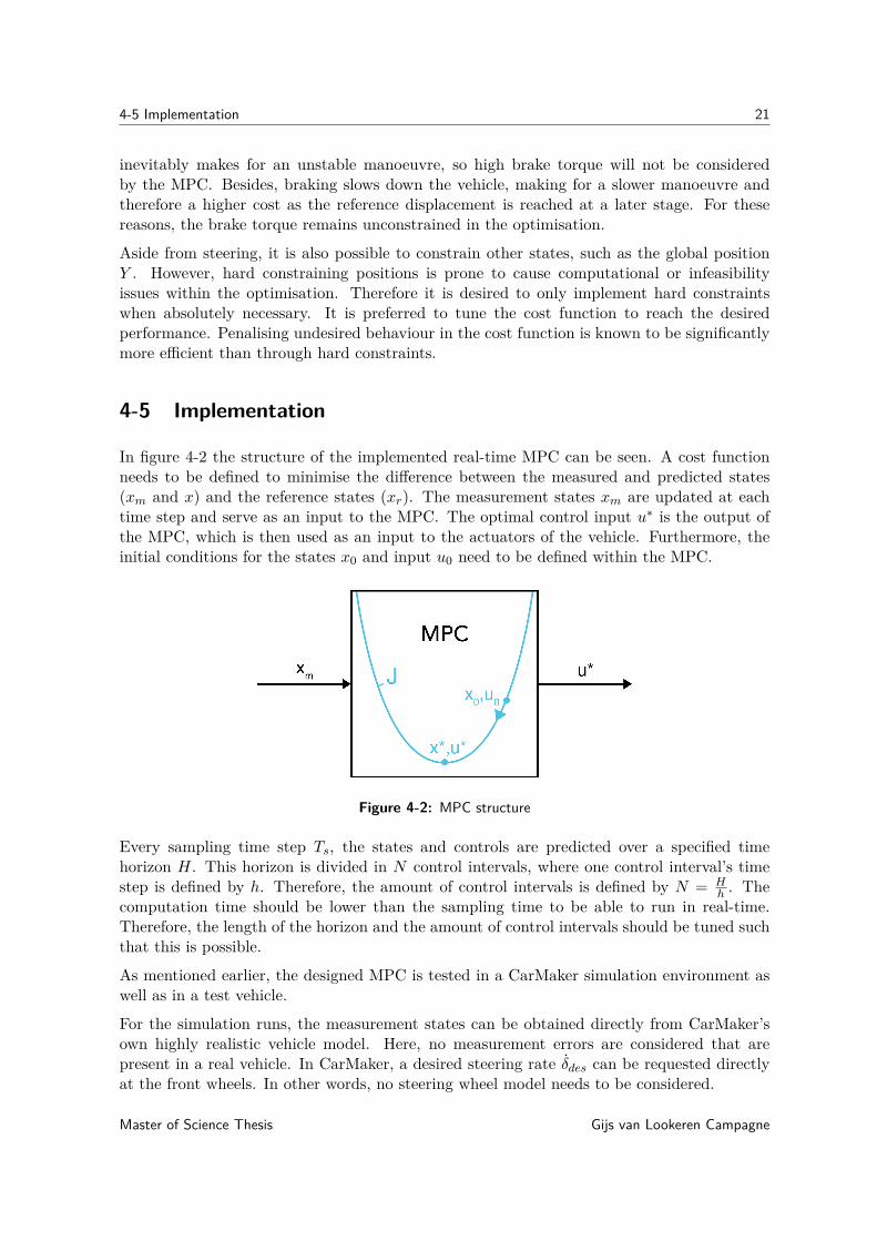
In figure 4-2 the structure of the implemented real-time MPC can be seen. A cost functionneeds to be defined to minimise the difference between the measured and predicted states(xm and x) and the reference states (xr). The measurement states xm are updated at eachtime step and serve as an input to the MPC. The optimal control input u∗ is the output ofthe MPC, which is then used as an input to the actuators of the vehicle. Furthermore, theinitial conditions for the states x0 and input u0 need to be defined within the MPC.
Figure 4-2: MPC structure
Every sampling time step Ts, the states and controls are predicted over a specified timehorizon H. This horizon is divided in N control intervals, where one control interval’s timestep is defined by h. Therefore, the amount of control intervals is defined by N = H
h . Thecomputation time should be lower than the sampling time to be able to run in real-time.Therefore, the length of the horizon and the amount of control intervals should be tuned suchthat this is possible.
As mentioned earlier, the designed MPC is tested in a CarMaker simulation environment aswell as in a test vehicle.
For the simulation runs, the measurement states can be obtained directly from CarMaker’sown highly realistic vehicle model. Here, no measurement errors are considered that arepresent in a real vehicle. In CarMaker, a desired steering rate δdes can be requested directlyat the front wheels. In other words, no steering wheel model needs to be considered.
Master of Science Thesis Gijs van Lookeren Campagne

22 Model Predictive Control
Figure 4-3: Sampling times within MPC
During experimental tests, challenges arise that were not present during simulation runs.First and foremost, C code needs to be built so that the MPC can be employed on thedSPACE system in the test vehicle. Secondly, the measurement signals measured by theInertial Measurement Unit (IMU) are not as accurate as the measurement signals in thesimulation environment. This provides a challenge for the MPC in terms of robustness.Lastly, a sufficiently accurate representation of a steering wheel torque model needs to bederived. This allows to map the requested steering rate to a requested steering torque. Thisway, the actuator is able to track the desired steering rate computed by the MPC. A schematicoverview of the simulation and experimental setup can be observed in 4-4.
Figure 4-4: Schematic overview of simulation and experimental setup
Gijs van Lookeren Campagne Master of Science Thesis
Chapter 5
Nonlinear programming
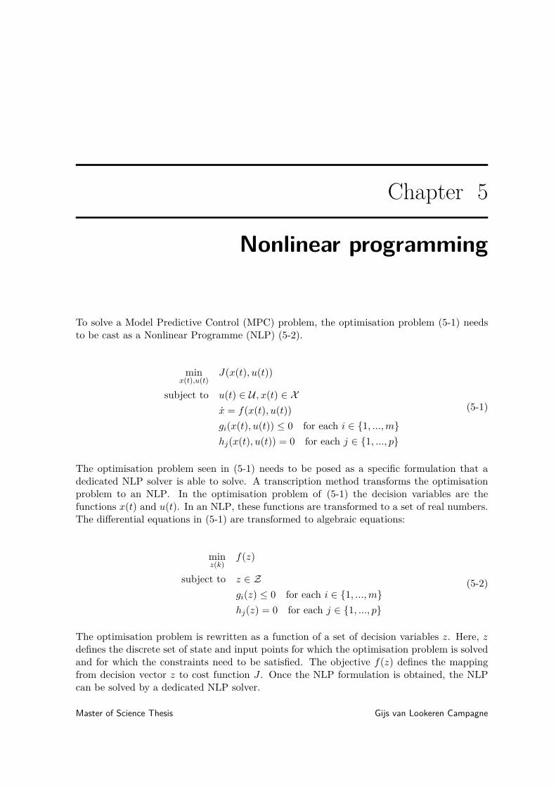
To solve a Model Predictive Control (MPC) problem, the optimisation problem (5-1) needsto be cast as a Nonlinear Programme (NLP) (5-2).
minx(t),u(t)
J(x(t), u(t))
subject to u(t) ∈ U , x(t) ∈ Xx = f(x(t), u(t))gi(x(t), u(t)) ≤ 0 for each i ∈ {1, ...,m}hj(x(t), u(t)) = 0 for each j ∈ {1, ..., p}
(5-1)
The optimisation problem seen in (5-1) needs to be posed as a specific formulation that adedicated NLP solver is able to solve. A transcription method transforms the optimisationproblem to an NLP. In the optimisation problem of (5-1) the decision variables are thefunctions x(t) and u(t). In an NLP, these functions are transformed to a set of real numbers.The differential equations in (5-1) are transformed to algebraic equations:
minz(k)
f(z)
subject to z ∈ Zgi(z) ≤ 0 for each i ∈ {1, ...,m}hj(z) = 0 for each j ∈ {1, ..., p}
(5-2)
The optimisation problem is rewritten as a function of a set of decision variables z. Here, zdefines the discrete set of state and input points for which the optimisation problem is solvedand for which the constraints need to be satisfied. The objective f(z) defines the mappingfrom decision vector z to cost function J . Once the NLP formulation is obtained, the NLPcan be solved by a dedicated NLP solver.
Master of Science Thesis Gijs van Lookeren Campagne

24 Nonlinear programming
In this chapter, two approaches to solving the MPC problem will be presented. The firstapproach is an Interior-Point Method (IPM) using the IPOPT [28] solver. Here, the stateand control trajectories are transcribed using a direct collocation method. The open-sourcepackage CasADi [29] is used to implement and solve the NLP. As explained previously, thisapproach will only be tested in simulation.
A Sequential Quadratic Programming (SQP) method is implemented using the qpOASES [30]solver in the open-source package ACADO [31]. This approach will be tested in simulationas well as during real-life tests on an embedded dSPACE MicroAutobox II setup in a VolvoV40 test car.
An overview of both approaches can be seen in table 5-1:
Table 5-1: Overview of approaches for solving the NLP
Solver Transcription method Framework Simulation TestsI. IPOPT (IPM) Direct Collocation CasADi Yes NoII. qpOASES (SQP) Multiple Shooting ACADO Yes Yes
CasADi (IPOPT/Direct collocation) is known to be faster for larger problems (a high numberof states) [32]. Smaller to medium sized problems are likely to be solved faster by ACADOusing SQP and a multiple shooting method. Problem size varies for different experimentsthroughout this thesis. In practice, this means that lower fidelity vehicle models are likely toperform better using ACADO (and SQP) and higher fidelity models will probably performbetter using CasADi (and IPM). SQP is known to be better at handling highly (hard)constrained problems. A comparison between both CasADi and ACADO will provide insightin which framework will suit the scope of this thesis better. Both methods will make use ofso-called warm-starts to initialise at each iteration. This means that the previous optimalsolution is used as the initial condition for the next time step. Generally, the previous solutionproves to be a good initial guess for the next time step.
5-1 Transcription methods
Transcription methods for optimal control can be categorised in different groups. First off,there are direct and indirect methods. In direct methods, the problem is first discretised andthen optimised. In indirect methods, the necessary conditions for optimality are calculatedfirst. Then, these conditions are discretised and solved. The transcription methods consideredin this thesis, rely on direct transcription. Indirect transcription methods are very accurate,but hard to solve in practice as they require very accurate initial guesses to converge [33].
Direct methods can be divided in simultaneous and sequential approaches. A single shootingmethod is an example of a sequential method. In this method, only the control trajectoriesare discretised, by a piecewise smooth approximation. The discretised control trajectoriesthen enter the NLP. A single shooting method can be compared to a cannon shooting at atarget. First, an estimate is made of a good shooting angle. Then it is checked whether thetarget has been hit. If not, the angle is adjusted based on the previous result so that the
Gijs van Lookeren Campagne Master of Science Thesis

5-1 Transcription methods 25
problem is solved sequentially using multiple iterations. The resulting NLP using a singleshooting method is generally a smaller sized problem, but highly nonlinear [34].
Convergence can be improved by considering a Multiple shooting method, where the problemsize is bigger, but includes less nonlinearities. Compared to a single shooting method, amultiple shooting method typically results in better convergence of NLPs and a higher degreeof numerical stability (i.e. less sensitive to errors due to e.g. poorly chosen initial guesses)[35]. Furthermore, the resulting NLP has a sparser structure that can be exploited [34]. In amultiple shooting method, not only the control trajectories are discretised, but also the statetrajectories. A direct collocation method results in an even larger NLP, but yields an evensparser structure compared to multiple shooting. Both the multiple shooting method anddirect collocation method are explained in more detail in the next subsections.
The decision variables in this chapter are hereafter denoted by x.
5-1-1 Multiple Shooting method
A shooting method is a transcription method that is based on simulation. Typically, a Runga-Kutta scheme is used to obtain the discrete-time dynamics. In Multiple shooting methodsonly the states and control inputs at the beginning of each control interval are included. Thereare no intermediate collocation points as seen in the direct collocation method.
In figure 5-1 the multiple shooting method is shown graphically. First, the continuous (5-1a)state and control trajectories are discretised (5-1b). The amount of control intervals is denotedby N . The control inputs u(t) are discretised to obtain the decision variables u0, u1, . . . , uN−1:
u(t) = uk, for t ∈ [tk, tk+1], k = 0, . . . , N − 1 (5-3)
Similarly, the state decision variables x0, x1, . . . , xN are are defined. Now, every interval kconsists of a control signal uk and a start state xk, as shown in figure 5-1b. Starting from xkand by integrating over each interval, the state at the next interval xk+1 can be determined.
(a) Continuous state and control (b) Discretised state and control (c) Integrated state trajectories
Figure 5-1: Multiple shooting method
In figure 5-1c it can be seen that there is a mismatch between the state obtained by integratingand the start state of the next time step. Continuity constraints are added to make sure thatthere is no mismatch between these two states:
Master of Science Thesis Gijs van Lookeren Campagne

26 Nonlinear programming
xk+1 − xk+1 = 0 (5-4)
In this thesis, a Runge-Kutta approach is used to obtain the state at the next time step xk+1.Runge-Kutta methods are a class of methods to integrate ordinary differential equations. Inthis case, a fourth order Runge-Kutta method is employed. It approximates the solutionto a differential equation x = f(t, x) with initial condition x(t0) = x0. The order of theRunge-Kutta method refers to the amount of approximations of the slope within one timestep. In figure 5-2 a visualisation for the fourth order Runge-Kutta method can be observed.The slope at the start point and end point are defined by R1 and R4. The slopes at the twomidpoints are R2 and R3.
Figure 5-2: Fourth order Runge-Kutta method
To determine an approximation of xk+1, a weighted average of the slopes at R1, R2, R3 andR4 is used:
xk+1 = xk + 16(R1 + 2R2 + 2R3 +R4)h
tk+1 = tk + h(5-5)
The midpoint slopes are weighted twice as much as the start and end point. The individualslopes at each point are defined as:
R1 = f(tk, xk)R2 = f(tk + h/2, xk +R1/2)R3 = f(tk + h/2, xk +R2/2)R4 = f(tk + h, xk +R3)
(5-6)
Gijs van Lookeren Campagne Master of Science Thesis
5-1 Transcription methods 27
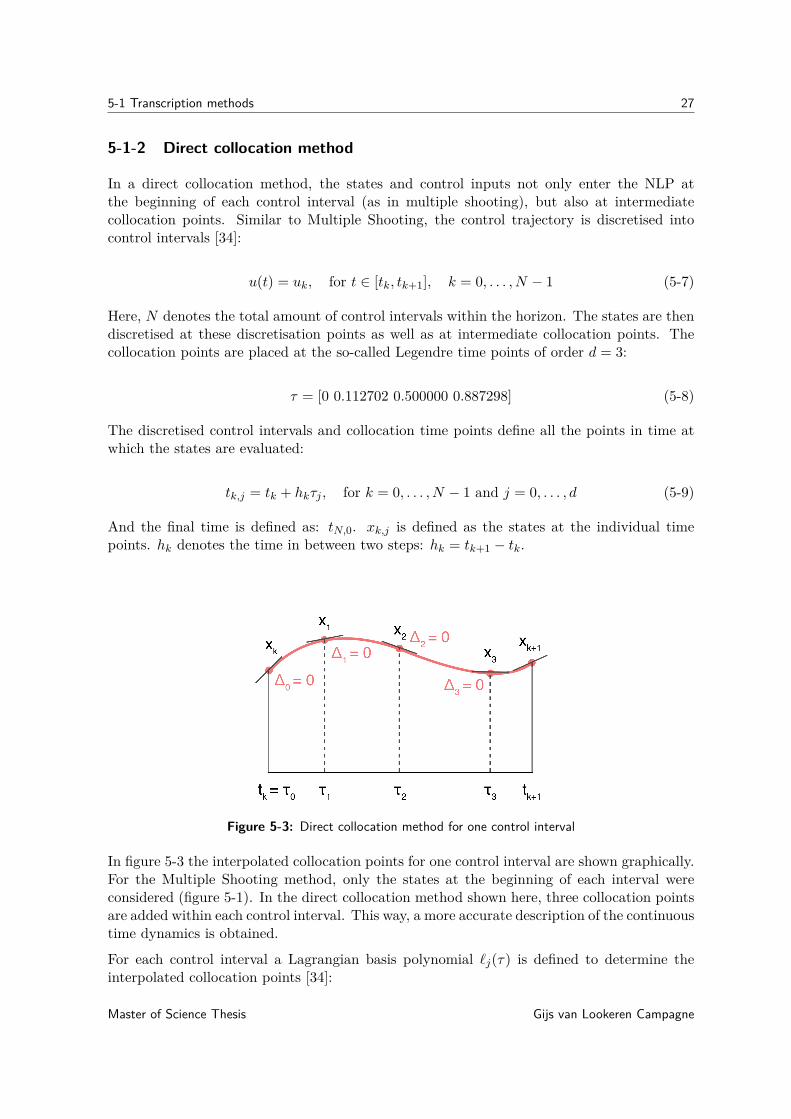
5-1-2 Direct collocation method
In a direct collocation method, the states and control inputs not only enter the NLP atthe beginning of each control interval (as in multiple shooting), but also at intermediatecollocation points. Similar to Multiple Shooting, the control trajectory is discretised intocontrol intervals [34]:
u(t) = uk, for t ∈ [tk, tk+1], k = 0, . . . , N − 1 (5-7)
Here, N denotes the total amount of control intervals within the horizon. The states are thendiscretised at these discretisation points as well as at intermediate collocation points. Thecollocation points are placed at the so-called Legendre time points of order d = 3:
τ = [0 0.112702 0.500000 0.887298] (5-8)
The discretised control intervals and collocation time points define all the points in time atwhich the states are evaluated:
tk,j = tk + hkτj , for k = 0, . . . , N − 1 and j = 0, . . . , d (5-9)
And the final time is defined as: tN,0. xk,j is defined as the states at the individual timepoints. hk denotes the time in between two steps: hk = tk+1 − tk.
Figure 5-3: Direct collocation method for one control interval
In figure 5-3 the interpolated collocation points for one control interval are shown graphically.For the Multiple Shooting method, only the states at the beginning of each interval wereconsidered (figure 5-1). In the direct collocation method shown here, three collocation pointsare added within each control interval. This way, a more accurate description of the continuoustime dynamics is obtained.
For each control interval a Lagrangian basis polynomial `j(τ) is defined to determine theinterpolated collocation points [34]:
Master of Science Thesis Gijs van Lookeren Campagne

28 Nonlinear programming
`j(τ) =d∏
m=0,m 6=j
τ − τmτj − τm
(5-10)
`j(τ) =d∏
m=0,m 6=j
τ − τmτj − τm
= τ − τ0τj − τ0
. . .τ − τj−1τm − τj−1
τ − τj+1τm − τj+1
. . .τ − τd−1τm − τd−1
(5-11)
`j(τm) ={
1, if j = m
0, otherwise(5-12)
The states can then be approximated as a linear combination of the Lagrange basis polyno-mials:
xk(t) =d∑
m=0`m
(t− tkhk
)xk,m (5-13)
The approximations of the state derivatives at the individual collocations points (except atτ0) are:
˜xk(tk,j) = 1hk
d∑m=0
˙m(τj)xk,m (5-14)
The state at the end of a control interval is defined as:
xk+1,0 =d∑
m=0`m(1)xk,m (5-15)
To ensure that the state derivatives are approximated correctly the so-called collocation equa-tions enter the NLP as a constraint (as shown in figure 5-3):
∆k,j = hkf(tk,j , xk,j , uk)−d∑
m=0
˙m(τj)xk,m = 0, for k = 0, . . . , N−1 and j = 1, . . . , d (5-16)
Furthermore, the approximated end state enters the NLP as well to ensure that the states atthe next time step are equal to the state at the end of the previous time step:
xk+1,0 −d∑
m=0`m(1)xk,m = 0, k = 0, . . . , N − 1 (5-17)
Gijs van Lookeren Campagne Master of Science Thesis

5-2 Sequential Quadratic Programming 29
5-2 Sequential Quadratic Programming
Now that both transcription methods have been defined, NLP methods are considered tosolve the posed optimisation problem.In SQP an NLP is modelled as a Quadratic Programming (QP) subproblem at each iterationxk. This subproblem is then solved to find the next iteration xk+1 [36]. This process isiterated to find an optimal solution x∗. In contrast to to IPM, in SQP the iterations donot require to be feasible. The NLP solver that is used is qpOASES [30]. It incorporatestwo established algorithms in nonlinear optimisation: The Active Set method and Newton’smethod.SQP aims to solve the following general optimisation problem:
minx∈Rn
f(x)
subject to h(x) = 0g(x) ≤ 0
(5-18)
ACADO allows for condensed formulation of the system dynamics to decrease the compu-tational complexity. In this condensed formulation the states of the decision variables areeliminated and evaluated as a function of the current time states and future time controlinputs [37].In SQP the next iteration is found by solving a quadratic subproblem of the form [36]:
mindx
k
(rk)Tdxk + 12(dxk)TBkdxk
subject to ∇h(xk)Tdxk + h(xk) = 0∇g(xk)Tdxk + g(xk) ≤ 0
(5-19)
.Here, dx = x − xk. Now, rk and Bk need to be chosen such that the subproblem reflectsthe original problem. This can be done by taking the local quadratic approximation of f atxk, resulting in setting rk to be equal to the gradient of f at point xk. Bk is chosen as theHessian of f at point xk, ∇2
xxL(xk, λk, νk), but is approximated by a Gauss-Newton Hessianapproximation. For an objective of f(x) = ||r(x)||22 the Gauss-Newton Hessian becomes [38]:
Bk = 2∇xr(xk)∇xr(xk)T (5-20)
A Lagrangian function incorporates all information of the optimisation problem in 5-18 intoone function:
L(x, λ, ν) = f(x) + λTh(x) + νT g(x) (5-21)
Here, λ ∈ Rp and ν ∈ Rm are the Lagrange multipliers for the equality and inequalityconstraints, respectively. The Lagrangian multipliers denote the change in the objective
Master of Science Thesis Gijs van Lookeren Campagne

30 Nonlinear programming
function with respect to a change in the respective constraints. SQP uses a quadratic modelof the Lagrangian function as the objective to be minimised, such that the nonlinearities ofthe original problem are captured [36]:
minx
L(x, λ∗, ν∗)
subject to h(x) = 0g(x) ≤ 0
(5-22)
where λ∗ and v∗ denote the optimal multipliers. As the optimal multipliers are unknown,approximations λk and vk can be used instead. The quadratic Taylor-series approximation ofthe Lagrangian in x is used as the objective function instead of the original objective function[36]. The advantage of this function is that its iterations are identical to iterations generatedusing Newton’s method. The quadratic Taylor-series approximation of the Lagrangian is:
L(xk, λk, νk) +∇L(xk, λk, νk)Tdxk + 12(dxk)THL(xk, λk, νk)dxk (5-23)
The gradient of the Lagrangian forms the following system and is equivalent to the Karush-Kuhn-Tucker Conditions (KKT) conditions:
∇L(x, λ, ν) =
dLdxdLdλdLdν
=
∇f + λ∇h+ ν∇g∗hg∗
(5-24)
As mentioned previously the first term contains the optimisation problem of (5-18), whichis minimised by regarding its derivative and setting this term equal to zero. The secondKKT condition is there to ensure feasibility, as h(x) = 0 is a constraint imposed in theoriginal optimisation problem. In the third KKT condition, the active set is denoted by g∗.The KKT conditions need to be met for the solution to be considered optimal [39]. As SQPincorporates an active set strategy only active inequality constraints are taken into account forthe optimisation. This means that inequality constraints far away from the optimal solutionare temporarily ignored and are called inactive. When an inequality constraint is violated,this inequality constraint becomes active and may be treated as an equality constraint. Usingbacktracking, the step length α is chosen such that solution is on the boundary of the feasibleregion again.
In figure 5-4 the procedure for a simple example of the active set method is shown. In mostcases, the optimal solution lies on the boundary of the feasible set, as in the example shownbelow. In the case where the optimal solution lies within the feasible set, all Lagrangianmultipliers disappear and the problem will be solved as if it is unconstrained.
At the initial point x0 = (0, 0) (I) the green (−x1 + x2 ≤ 0) and red (x2 ≥ 0) inequalityconstraints become active. The blue constraint (x1 + x2 ≤ 1) remains inactive at the initialpoint. When the step length is too large, the next iteration could end up outside of the feasibleset (II). Therefore the step length needs to be chosen such that it is as large as possible butthe next iteration remains within the feasible set (III). This can be achieved by means of
Gijs van Lookeren Campagne Master of Science Thesis

5-2 Sequential Quadratic Programming 31
backtracking. In point III the blue and red constraint become active and the green constraintbecomes inactive. Then it is checked whether the Lagrange multiplier for both constraintsare positive. When the Lagrange multiplier is negative, the constraint associated with thatmultiplier is dropped and becomes inactive. In this case, the Lagrange multiplier for thered constrained is negative, resulting in this constrained being dropped. When the Lagrangemultipliers for all active constraints are positive, the associated point is the optimal solution.The latter is the case for point IV and therefore an optimal solution is found here.
(a) Initial point (b) Backtracking (c) Optimal solution
Figure 5-4: Optimal solution
The Hessian of the Lagrangian is defined as:
HL(x, λ, µ) =
∇2xxL(x, λ, ν) ∇h ∇g∇h 0 0∇g 0 0
(5-25)
The quadratic subproblem can then be rewritten as:
mindx
∇L(xk, λk, νk)Tdxk + 12(dxk)TBkdxk
subject to ∇h(xk)Tdxk + h(xk) = 0∇g(xk)Tdxk + g(xk) ≤ 0
(5-26)
.
At iteration k, the NLP (5-2) can be cast as the following quadratic subproblem:
mindx
k
∇f(xk)Tdxk + 12(dxk)TBkdxk
subject to ∇h(xk)Tdxk + h(xk) = 0∇g(xk)Tdxk + g(xk) ≤ 0
(5-27)
Equations (5-26) and (5-27) are equivalent when there are only equality constraints. In thecase of inequality constraints they are equivalent if the NLP is posed using slack variables s:
Master of Science Thesis Gijs van Lookeren Campagne

32 Nonlinear programming
minx∈Rn,d∈Rp
f(x)
subject to h(x) = 0g(x) + s = 0s ≥ 0
(5-28)
The solution dx found by solving the QP in (5-27) is then used to obtain a new iterate xk+1.Aside from defining xk+1, new Lagrangian multipliers λk+1 and νk+1 are needed for the nextiteration. The directions for the multipliers are defined as:
dλk = λqp − λkdvk = vqp − vk
(5-29)
Where λqp and νqp are the optimal Langange multipliers of the QP in (5-27). Then, asteplength parameter α needs to be chosen such that:
φ(xk + αdxk) ≤ φ(xk) (5-30)
Here, φ is a merit function. The purpose of the merit function is to track and measure theprogress of the optimisation, such that global convergence can be guaranteed. When thevalue of the merit function φ reduces, a step towards a solution has been taken. When theinequality in (5-30) holds for a time step k, the value of φ will be reduced for the next timestep. The step length α needs to be adjusted at each time step to guarantee a reduction of φat each time step.
The next iterates for x, λ and ν can then be written as:
xk+1 = xk + αdxk
λk+1 = λk + αdλk
νk+1 = νk + αdνk
(5-31)
When dxk is smaller than a set relative tolerance δ and the KKT conditions are met, thesolution has converged.
Gijs van Lookeren Campagne Master of Science Thesis
5-3 Interior-point Method 33
5-3 Interior-point Method
Aside from SQP, an Interior-Point Method (IPM) is used to solve the NLP shown in (5-2).The NLP solver that is used is IPOPT [28]. It incorporates a so-called Primal-Dual Barrierapproach. It allows to solve problems of the form:
minx∈Rn
f(x)
subject to c(x) = 0x ≥ 0
(5-32)
It also possible to define a lower bound for x here, but this is omitted for the sake of simplicity.A barrier method typically moves an inequality constraint to the cost function. It does so byincluding a logarithmic barrier term in the cost function:
minx∈Rn
φµ(x) = f(x)− µn∑i=1
ln(xi)
subject to c(x) = 0(5-33)
The parameter µ is used to penalise states being close to the barrier. When µ is decreasediteratively, the minimum is reached. This problem is equivalent to solving the primal-dualequations:
∇f(x) +∇c(x)λ− ν = 0c(x) = 0
XNe− µe = 0(5-34)
The primal-dual equations of (5-34) together with x, ν ≥ 0 denote the Karush-Kuhn-Tucker(KKT) conditions. X and N represent diagonal matrices with the indices of x and ν, respec-tively.
The first equation in (5-34) is the gradient of the Lagrangian function (5-35). The Lagrangianallows to combine all constraints and the function to be minimised in one function. Evaluatingwhere its gradient equals zero will therefore yield the minimum.
L(x, µ, z) = f(x) + c(x)Tλ− ν (5-35)
Here, λ ∈ Rm is a Lagrange multiplier that refers to the equality constraint c(x) = 0 in (5-32).The inequality constraint x ≥ 0 in (5-32) is incorporated by the Lagrange multiplier ν ∈ Rn.To speed up the iterative process of decreasing µ, Newton steps can be taken to approachthe optimum. The search directions dxk, dλk and dνk need to be found to find the next iterationxk+1, λk+1, νk+1:
Master of Science Thesis Gijs van Lookeren Campagne

34 Nonlinear programming
xk+1 = xk + αkdxk
λk+1 = λk + αkdλk
νk+1 = νk + αkdνk
(5-36)
Here, αk denotes the step size. The search directions are found by solving equation (5-37) fordxk, dλk and dνk: Wk Ak −I
ATk 0 0Nk 0 Xk
dxkdλkdνk
= −
∇f(xk) +Akλk − νkc(xk)
XkNke− µje
(5-37)
Here, Ak = ∇c(xk) and Wk is Hessian of the Lagrangian (5-35):
Wk = ∇2xxL(xk, λk, νk) = ∇2
xx(f(xk) + c(xk)Tλk − νk) (5-38)
Nk and Xk are defined as:
Nk =
ν1 0 0
0 . . . 00 0 νn
, Xk =
x1 0 0
0 . . . 00 0 xn
(5-39)
The nonsymmetric linear system (5-37) can be solved equivalently by solving a symmetriclinear system:
[Wk + Σk AkATk 0
] [dxkdλk
]= −
[∇φµj (xk) +Akλk
c(xk)
](5-40)
Where Σk = X−1k Nk. After having solved (5-40) for dxk and dλk , the search direction dzk can
be expressed as:
dzk = µjX−1k e− νk − Σkd
xk (5-41)
Gijs van Lookeren Campagne Master of Science Thesis
Chapter 6
Simulation results
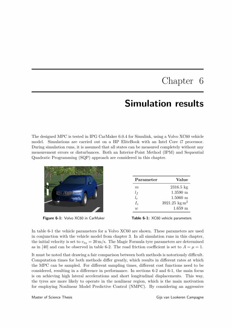
The designed MPC is tested in IPG CarMaker 6.0.4 for Simulink, using a Volvo XC60 vehiclemodel. Simulations are carried out on a HP EliteBook with an Intel Core i7 processor.During simulation runs, it is assumed that all states can be measured completely without anymeasurement errors or disturbances. Both an Interior-Point Method (IPM) and SequentialQuadratic Programming (SQP) approach are considered in this chapter.
Figure 6-1: Volvo XC60 in CarMaker
Parameter Valuem 2316.5 kglf 1.3590 mlr 1.5060 mIz 3921.25 kg m2
w 1.659 m
Table 6-1: XC60 vehicle parameters
In table 6-1 the vehicle parameters for a Volvo XC60 are shown. These parameters are usedin conjunction with the vehicle model from chapter 3. In all simulation runs in this chapter,the initial velocity is set to vx0 = 20 m/s. The Magic Formula tyre parameters are determinedas in [40] and can be observed in table 6-2. The road friction coefficient is set to A = µ = 1.
It must be noted that drawing a fair comparison between both methods is notoriously difficult.Computation times for both methods differ greatly, which results in different rates at whichthe MPC can be sampled. For different sampling times, different cost functions need to beconsidered, resulting in a difference in performance. In sections 6-2 and 6-1, the main focusis on achieving high lateral accelerations and short longitudinal displacements. This way,the tyres are more likely to operate in the nonlinear region, which is the main motivationfor employing Nonlinear Model Predictive Control (NMPC). By considering an aggressive
Master of Science Thesis Gijs van Lookeren Campagne
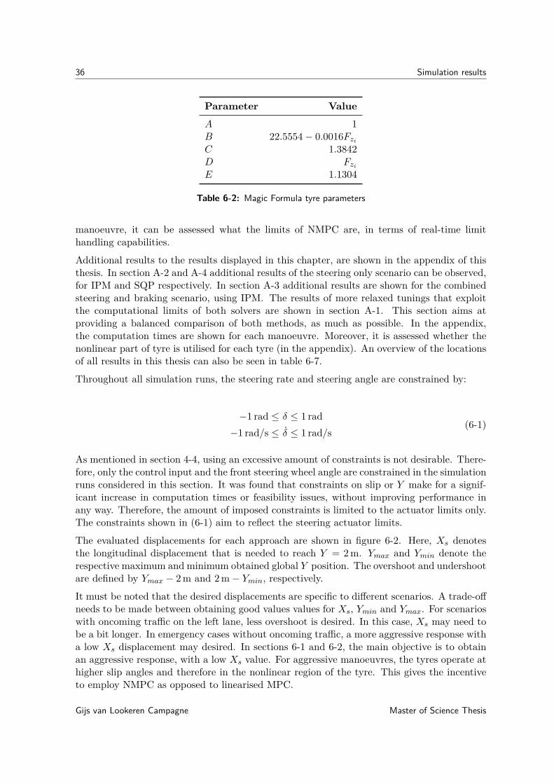
36 Simulation results
Parameter ValueA 1B 22.5554− 0.0016Fzi
C 1.3842D Fzi
E 1.1304
Table 6-2: Magic Formula tyre parameters
manoeuvre, it can be assessed what the limits of NMPC are, in terms of real-time limithandling capabilities.
Additional results to the results displayed in this chapter, are shown in the appendix of thisthesis. In section A-2 and A-4 additional results of the steering only scenario can be observed,for IPM and SQP respectively. In section A-3 additional results are shown for the combinedsteering and braking scenario, using IPM. The results of more relaxed tunings that exploitthe computational limits of both solvers are shown in section A-1. This section aims atproviding a balanced comparison of both methods, as much as possible. In the appendix,the computation times are shown for each manoeuvre. Moreover, it is assessed whether thenonlinear part of tyre is utilised for each tyre (in the appendix). An overview of the locationsof all results in this thesis can also be seen in table 6-7.
Throughout all simulation runs, the steering rate and steering angle are constrained by:
−1 rad ≤ δ ≤ 1 rad−1 rad/s ≤ δ ≤ 1 rad/s
(6-1)
As mentioned in section 4-4, using an excessive amount of constraints is not desirable. There-fore, only the control input and the front steering wheel angle are constrained in the simulationruns considered in this section. It was found that constraints on slip or Y make for a signif-icant increase in computation times or feasibility issues, without improving performance inany way. Therefore, the amount of imposed constraints is limited to the actuator limits only.The constraints shown in (6-1) aim to reflect the steering actuator limits.
The evaluated displacements for each approach are shown in figure 6-2. Here, Xs denotesthe longitudinal displacement that is needed to reach Y = 2 m. Ymax and Ymin denote therespective maximum and minimum obtained global Y position. The overshoot and undershootare defined by Ymax − 2 m and 2 m− Ymin, respectively.
It must be noted that the desired displacements are specific to different scenarios. A trade-offneeds to be made between obtaining good values values for Xs, Ymin and Ymax. For scenarioswith oncoming traffic on the left lane, less overshoot is desired. In this case, Xs may need tobe a bit longer. In emergency cases without oncoming traffic, a more aggressive response witha low Xs displacement may desired. In sections 6-1 and 6-2, the main objective is to obtainan aggressive response, with a low Xs value. For aggressive manoeuvres, the tyres operate athigher slip angles and therefore in the nonlinear region of the tyre. This gives the incentiveto employ NMPC as opposed to linearised MPC.
Gijs van Lookeren Campagne Master of Science Thesis

37
Figure 6-2: Trajectory layout
For all scenarios, the body slip β = atan(vy/vx) is evaluated. This is the slip measured at thecentre of gravity of the vehicle.
Master of Science Thesis Gijs van Lookeren Campagne
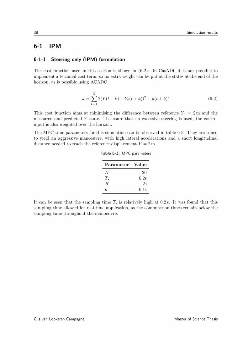
38 Simulation results
6-1 IPM
6-1-1 Steering only (IPM) formulation
The cost function used in this section is shown in (6-2). In CasADi, it is not possible toimplement a terminal cost term, so no extra weight can be put at the states at the end of thehorizon, as is possible using ACADO.
J =N∑k=1
2(Y (t+ k)− Yr(t+ k))2 + u(t+ k)2 (6-2)
This cost function aims at minimising the difference between reference Yr = 2 m and themeasured and predicted Y state. To ensure that no excessive steering is used, the controlinput is also weighted over the horizon.
The MPC time parameters for this simulation can be observed in table 6-3. They are tunedto yield an aggressive manoeuvre, with high lateral accelerations and a short longitudinaldistance needed to reach the reference displacement Y = 2 m.
Table 6-3: MPC parameters
Parameter ValueN 20Ts 0.2sH 2sh 0.1s
It can be seen that the sampling time Ts is relatively high at 0.2 s. It was found that thissampling time allowed for real-time application, as the computation times remain below thesampling time throughout the manoeuvre.
Gijs van Lookeren Campagne Master of Science Thesis

6-1 IPM 39
6-1-2 Steering & braking (IPM) formulation
In this section, the extended vehicle model of section 3-2-2 is used. The time parameters inthis scenario remain the same as was shown in table 6-3. The initial velocity also remains thesame at 20m/s. To incorporate the longitudinal wheel dynamics, the following parametersare defined:
Parameter ValueRw 0.365 mBd 1 Nms/radIwz 1.772 kg m2
Table 6-4: Longitudinal wheel parameters
For this problem a different cost function is used:
J =N∑k=1
5(Y (t+ k)− Yr(t+ k))2 + 10−3x(t+ k)2 + u(t+ k)TRu(t+ k) (6-3)
where the input weight matrix R is defined as:
R =
1 0 0 0 00 10−6 0 0 00 0 10−6 0 00 0 0 10−6 00 0 0 0 10−6
(6-4)
To force the MPC to use the brakes more, the longitudinal velocity is incorporated in the costfunction. Without this term, the MPC is not inclined to use the brakes. Braking slows downthe manoeuvre so it will take longer to reach the destination, thus increasing the cost overtime. Therefore, without this velocity term, the brakes are barely used. The cost functionshown here, was found to provide the maximum usage of the brakes, whilst still maintainingstability.
Master of Science Thesis Gijs van Lookeren Campagne
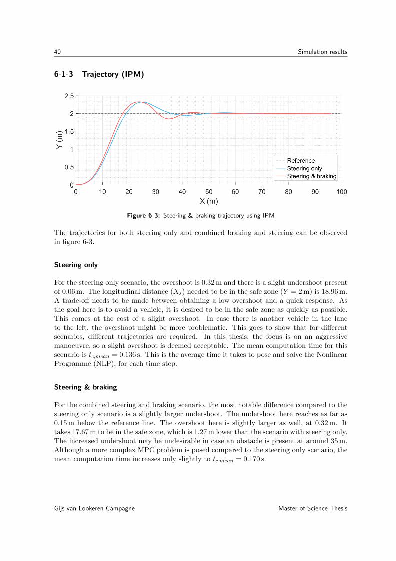
40 Simulation results
6-1-3 Trajectory (IPM)
Figure 6-3: Steering & braking trajectory using IPM
The trajectories for both steering only and combined braking and steering can be observedin figure 6-3.
Steering only
For the steering only scenario, the overshoot is 0.32 m and there is a slight undershoot presentof 0.06 m. The longitudinal distance (Xs) needed to be in the safe zone (Y = 2 m) is 18.96 m.A trade-off needs to be made between obtaining a low overshoot and a quick response. Asthe goal here is to avoid a vehicle, it is desired to be in the safe zone as quickly as possible.This comes at the cost of a slight overshoot. In case there is another vehicle in the laneto the left, the overshoot might be more problematic. This goes to show that for differentscenarios, different trajectories are required. In this thesis, the focus is on an aggressivemanoeuvre, so a slight overshoot is deemed acceptable. The mean computation time for thisscenario is tc,mean = 0.136 s. This is the average time it takes to pose and solve the NonlinearProgramme (NLP), for each time step.
Steering & braking
For the combined steering and braking scenario, the most notable difference compared to thesteering only scenario is a slightly larger undershoot. The undershoot here reaches as far as0.15 m below the reference line. The overshoot here is slightly larger as well, at 0.32 m. Ittakes 17.67 m to be in the safe zone, which is 1.27 m lower than the scenario with steering only.The increased undershoot may be undesirable in case an obstacle is present at around 35 m.Although a more complex MPC problem is posed compared to the steering only scenario, themean computation time increases only slightly to tc,mean = 0.170 s.
Gijs van Lookeren Campagne Master of Science Thesis

6-1 IPM 41
6-1-4 Notable results (IPM)
(a) Steering angle (b) Body slip angle
(c) Lateral acceleration (d) Longitudinal velocity
Figure 6-4: Results of steering & braking scenario using IPM
Steering only
The aggressiveness of the manoeuvre is apparent from the steering angle plot (6-4a), especiallyin the first segment where the car makes a left turn. The body slip is displayed in figure 6-4b.This is the slip angle, measured at the centre of gravity of the vehicle. The two bursts ofslip are the results of the two short consecutive turns. The lateral acceleration in figure 6-4creaches a maximum of 8.19 m/s2 and a minimum of −7.10 m/s2. At the end of the manoeuvrethe longitudinal velocity vx (6-4d) is 18.42 m/s.
Steering & braking
For the steering and braking scenario, the MPC tries to correct for the undershoot at aroundX = 35m. This can be seen from the steering angle output (6-4a) around the 1.4s mark,where the steering angle is much larger than in the steering only scenario. Much more slip(6-4b) is obtained is during the manoeuvre, especially during the right turn of the manoeuvre.The maximum value for ay is 8.64 m/s2. Due to increasing steering angle at the 1.4 s mark,a higher lateral acceleration (6-4c) is obtained (at 2 s) as the MPC is trying to correct for
Master of Science Thesis Gijs van Lookeren Campagne
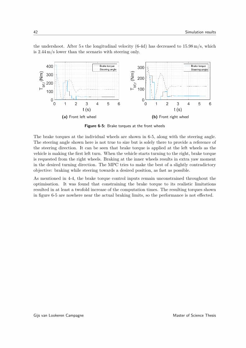
42 Simulation results
the undershoot. After 5 s the longitudinal velocity (6-4d) has decreased to 15.98 m/s, whichis 2.44 m/s lower than the scenario with steering only.
(a) Front left wheel (b) Front right wheel
Figure 6-5: Brake torques at the front wheels
The brake torques at the individual wheels are shown in 6-5, along with the steering angle.The steering angle shown here is not true to size but is solely there to provide a reference ofthe steering direction. It can be seen that brake torque is applied at the left wheels as thevehicle is making the first left turn. When the vehicle starts turning to the right, brake torqueis requested from the right wheels. Braking at the inner wheels results in extra yaw momentin the desired turning direction. The MPC tries to make the best of a slightly contradictoryobjective: braking while steering towards a desired position, as fast as possible.
As mentioned in 4-4, the brake torque control inputs remain unconstrained throughout theoptimisation. It was found that constraining the brake torque to its realistic limitationsresulted in at least a twofold increase of the computation times. The resulting torques shownin figure 6-5 are nowhere near the actual braking limits, so the performance is not effected.
Gijs van Lookeren Campagne Master of Science Thesis

6-2 SQP 43
6-2 SQP
6-2-1 Steering only (SQP) formulation
The steering only scenario is also evaluated using an SQP method. The MPC time parameters,shown in table 6-5 proved to yield good performance for the manoeuvre. The sampling timeis chosen to be much smaller, as an SQP approach results in relatively short computationtimes for this problem, compared to IPM.
Table 6-5: MPC parameters
Parameter ValueN 40Ts 0.04 sH 1.6 sh 0.04 s
The cost function, used in ACADO is the following:
J = 100(Y (N)− Yr(N))2 +N∑k=1
1 · 10−5(Y (t+ k)− Yr(t+ k))2 (6-5)
As mentioned before, ACADO allows for a terminal cost term that penalises the differencebetween the state and reference state at the end of the horizon. In this case, the weighton this terminal cost term is much higher than the weight on the states over the horizon.Decreasing the weight of the terminal cost term resulted in unsatisfactory performance usingSQP.
In this cost function there is no penalisation of the control input as the optimal control inputcalculated by the MPC was not found to be excessive. Furthermore, hard constraints ensurethat the control input stays within reasonable bounds.
A shifting strategy is incorporated for the SQP method. With a shifting strategy, the pre-dicted states are shifted one time step forward and used as an initial guess, essentially warmstarting the optimisation to increase convergence rates. The downside of a shifting strategyis that a delay block needs to be implemented to prevent an algebraic loop, delaying themanoeuvre by one sampling time step Ts. The slight delay with lower computation timesis favoured over no delay with higher computation times. Therefore, a shifting strategy isincluded.
Master of Science Thesis Gijs van Lookeren Campagne
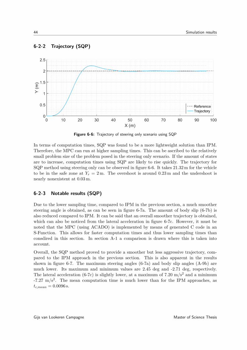
44 Simulation results
6-2-2 Trajectory (SQP)
Figure 6-6: Trajectory of steering only scenario using SQP
In terms of computation times, SQP was found to be a more lightweight solution than IPM.Therefore, the MPC can run at higher sampling times. This can be ascribed to the relativelysmall problem size of the problem posed in the steering only scenario. If the amount of statesare to increase, computation times using SQP are likely to rise quickly. The trajectory forSQP method using steering only can be observed in figure 6-6. It takes 21.32 m for the vehicleto be in the safe zone at Yr = 2 m. The overshoot is around 0.23 m and the undershoot isnearly nonexistent at 0.03 m.
6-2-3 Notable results (SQP)
Due to the lower sampling time, compared to IPM in the previous section, a much smoothersteering angle is obtained, as can be seen in figure 6-7a. The amount of body slip (6-7b) isalso reduced compared to IPM. It can be said that an overall smoother trajectory is obtained,which can also be noticed from the lateral acceleration in figure 6-7c. However, it must benoted that the MPC (using ACADO) is implemented by means of generated C code in anS-Function. This allows for faster computation times and thus lower sampling times thanconsdired in this section. In section A-1 a comparison is drawn where this is taken intoaccount.
Overall, the SQP method proved to provide a smoother but less aggressive trajectory, com-pared to the IPM approach in the previous section. This is also apparent in the resultsshown in figure 6-7. The maximum steering angles (6-7a) and body slip angles (A-9b) aremuch lower. Its maximum and minimum values are 2.45 deg and -2.71 deg, respectively.The lateral acceleration (6-7c) is slightly lower, at a maximum of 7.20 m/s2 and a minimum-7.27 m/s2. The mean computation time is much lower than for the IPM approaches, astc,mean = 0.0096 s.
Gijs van Lookeren Campagne Master of Science Thesis

6-3 Overview of simulation results 45
(a) Steering angle (b) Body slip angle
(c) Lateral acceleration (d) Longitudinal velocity
Figure 6-7: Results of steering only scenario using SQP
6-3 Overview of simulation results
An overview of the results of all scenarios and tunings, considered in simulation runs, is shownin table 6-7. The main differences between CasADi and ACADO, as found in this thesis, areillustrated in table 6-6.
It was found that the IPM approach in this thesis scaled better with problem size. A combinedsteering and braking scenario was implemented successfully, with only a slight increase incomputation times compared to a steering only scenario. The combined steering and brakingscenario involved an addition of 4 states, 4 control inputs and longitudinal dynamics. However,computation times remained in the same order of magnitude.
Remarkably, the more relaxed (steering only) tuning (section A-1) for IPM yielded a lowervalue for Xs than the aggressive tuning in section 6-1, while a lower maximum lateral accel-eration was obtained. This can be attributed to the excessive amount of slip present in thetuning found in 6-1.
For SQP, a combined steering and braking scenario could not be carried out. Compilationtimes for the C coded S-Function increased from around 5 minutes to around 2 hours, reducingthe ease of repeatability for different tunings. In most cases, the vehicle would not convergeto the desired lateral displacement at all. In other cases, the brakes were barely used (Tbi
<1 Nm). No tuning was found for which the combined steering and braking scenario could be
Master of Science Thesis Gijs van Lookeren Campagne
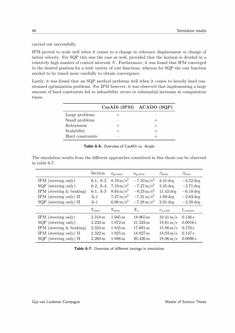
46 Simulation results
carried out successfully.
IPM proved to scale well when it comes to a change in reference displacement or change ofinitial velocity. For SQP this was the case as well, provided that the horizon is divided in arelatively high number of control intervals N . Furthermore, it was found that IPM convergedto the desired position for a wide variety of cost functions, whereas for SQP the cost functionneeded to be tuned more carefully to obtain convergence.
Lastly, it was found that an SQP method performs well when it comes to heavily hard con-strained optimisation problems. For IPM however, it was observed that implementing a largeamount of hard constraints led to infeasibility errors or substantial increases in computationtimes.
CasADi (IPM) ACADO (SQP)Large problems + –Small problems – +Robustness + ◦Scalability + +Hard constraints – +
Table 6-6: Overview of CasADi vs. Acado
The simulation results from the different approaches considered in this thesis can be observedin table 6-7.
Section ay,max ay,min βmax βmin
IPM (steering only) 6-1, A-2 8.19 m/s2 −7.10 m/s2 3.41 deg −4.52 degSQP (steering only) 6-2, A-4 7.19 m/s2 −7.27 m/s2 2.45 deg −2.71 degIPM (steering & braking) 6-1, A-3 8.64 m/s2 −8.23 m/s2 11.42 deg −6.10 degIPM (steering only) II A-1 7.27 m/s2 −7.21 m/s2 1.89 deg −2.63 degSQP (steering only) II A-1 6.98 m/s2 −7.28 m/s2 2.01 deg −2.28 deg
Ymax Ymin Xs vx,end tc,mean
IPM (steering only) 2.318 m 1.945 m 18.965 m 18.41 m/s 0.136 sSQP (steering only) 2.232 m 1.972 m 21.322 m 18.61 m/s 0.0016 sIPM (steering & braking) 2.324 m 1.845 m 17.691 m 15.98 m/s 0.170 sIPM (steering only) II 2.322 m 1.925 m 18.827 m 18.03 m/s 0.147 sSQP (steering only) II 2.260 m 1.986 m 20.426 m 18.06 m/s 0.0096 s
Table 6-7: Overview of different tunings in simulation
Gijs van Lookeren Campagne Master of Science Thesis
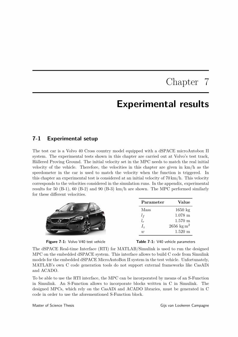
Chapter 7
Experimental results
7-1 Experimental setup
The test car is a Volvo 40 Cross country model equipped with a dSPACE microAutobox IIsystem. The experimental tests shown in this chapter are carried out at Volvo’s test track,Hällered Proving Ground. The initial velocity set in the MPC needs to match the real initialvelocity of the vehicle. Therefore, the velocities in this chapter are given in km/h as thespeedometer in the car is used to match the velocity when the function is triggered. Inthis chapter an experimental test is considered at an initial velocity of 70 km/h. This velocitycorresponds to the velocities considered in the simulation runs. In the appendix, experimentalresults for 50 (B-1), 60 (B-2) and 90 (B-3) km/h are shown. The MPC performed similarlyfor these different velocities.
Figure 7-1: Volvo V40 test vehicle
Parameter ValueMass 1650 kglf 1.078 mlr 1.570 mIz 2656 kg m2
w 1.520 m
Table 7-1: V40 vehicle parameters
The dSPACE Real-time Interface (RTI) for MATLAB/Simulink is used to run the designedMPC on the embedded dSPACE system. This interface allows to build C code from Simulinkmodels for the embedded dSPACEMicroAutoBox II system in the test vehicle. Unfortunately,MATLAB’s own C code generation tools do not support external frameworks like CasADiand ACADO.
To be able to use the RTI interface, the MPC can be incorporated by means of an S-Functionin Simulink. An S-Function allows to incorporate blocks written in C in Simulink. Thedesigned MPCs, which rely on the CasADi and ACADO libraries, must be generated in Ccode in order to use the aforementioned S-Function block.
Master of Science Thesis Gijs van Lookeren Campagne

48 Experimental results
As of today, CasADi supports code generation for everything except for the Nonlinear Pro-gramme (NLP) solver itself. It is possible to generate code that is dependent on libraries (inthis case CasADi and IPOPT). The libraries then need to be linked on the embedded system.As the dSPACE RTI only supports generated code from its MATLAB/Simulink interface(using S-Functions), the CasADi generated MPC can not be compiled for the embedded sys-tem. An alternative is to compile the CasADi core and IPOPT from source on the embeddedsystem.
ACADO on the other hand, supports full C code generation. The generated C code forMPC can be implemented in Simulink through an S-Function block. The C code needs tobe adjusted as some parts of ACADO are incompatible with dSPACE (such as internal timerrelated functions and print messages). After the C code is adjusted and an S-Function isbuilt, the entire controller can be built for the embedded system using the RTI.
Due to the slightly more user friendly way of embedding C code using ACADO, only thisapproach is tested in the test vehicle. CasADi and ACADO are compared in simulation andit is expected that their difference in performance should be similar in physical tests. Thecomplete code generation procedure is shown schematically in figure 7-2.
Figure 7-2: Code generation procedure
In the test scenario, the function will be triggered manually. In reality, the Evasive ManoeuvreAssistance Function (EMA) function is triggered when a set of conditions are met. As somecurrent Volvo models are already equipped with EMA functions, these triggering conditionsare already in place. During the test drives, Electronic Stability Control (ESC) was turnedoff.
The tyre model parameters for the test vehicle are unknown. Therefore, the same tyre modelparameters are used as during simulation runs. This introduces a mismatch between the tyremodel within the MPC and the real-life tyre behaviour and poses a challenge to the robustnessof the MPC.
Due to the fact that timer related functions are incompatible with the used dSPACE system,they are disabled. Therefore, no computation times can considered for the experimental tests.It was found however, that a sampling frequency of 25 Hz never resulted in any task overrunerrors. Task overrun errors occur when the dSPACE system is carrying out a task while thenext task is already scheduled to start. In other words, the computation time is higher thanthe sampling time and a real-time application is not possible. When a task overrun errorsoccurs, the designed software need to be reflashed on the MicroAutoBox to be able to testagain, which is time consuming. Due to the fact that repeatability was important to tune the
Gijs van Lookeren Campagne Master of Science Thesis

7-1 Experimental setup 49
MPC properly, the sampling frequency is set at 25 Hz for all experimental tests in this thesis,even though it may be possible to run at higher frequencies in some instances.
Master of Science Thesis Gijs van Lookeren Campagne

50 Experimental results
7-2 Obtaining the measurement states
During testing, measurement signals from the on-board Inertial Measurement Unit (IMU)are used. A Controller Area Network (CAN) bus is used for communication between theactuators, the AutoBox and the sensors.
The states that are measured by the IMU are: x, αr and ψ. Here, αr denotes the slip anglemeasured at the rear axle. From these states, y can be obtained:
y = x tanαr + ψlr (7-1)
X = x cosψ − y sinψY = x sinψ + y cosψ
(7-2)
By integrating X and Y the global positions X and Y are obtained. Measured signals areinevitably subject to noise with a slight bias resulting in so-called drift when the signal isintegrated. Over longer periods of time, this will result in a significant mismatch betweenmeasured state and the true state. In order to reduce the influence of drift on the measure-ments, the integrators will start from a set initial condition every time the evasive manoeuvrefunction is triggered. This ensures that there is no build-up of the integrator’s output priorto the function activation.
7-3 Torque request
During simulation runs in the previous section, it was possible to request a desired steeringangle at the steering wheel. In the test vehicle, steering wheel torque is requested as opposedto steering angle. To map steering rate or angle to steering wheel torque, a steering modelneeds to be developed. A steering model typically relies on accurately estimated parameterssuch as the torsion bar stiffness and steering column damping [41].
Torque can be requested by a so-called Driver Steering Recommendation (DSR) torque requestthat is sent to the MicroAutoBox. DSR is in place to assist the driver in difficult handlingsituations by giving a slight nudge on the steering wheel to recommend the driver to turnthe steering wheel. This nudge is given by a torque offset on the steering wheel in therecommended direction. Normally, the DSR torque request is limited at 3Nm for ordinarydriving and at 5Nm for the autopilot function. In the V40 test vehicle these limits are turnedoff and the actuator is limited by 7Nm. This is the maximum amount of Torque that ispossible to request through the MicroAutoBox.
A complex relation exists between wheel angle and applied torque at the steering wheels, dueto the presence of a power steering module. Boost curves are used to convert driver appliedtorque to a total amount of torque on the pinion, which is then translated to a displacementof the rack. When the rack is displaced, the wheels turn accordingly. The assistance torque isdependent on the vehicle velocity and the driver applied torque. As advanced steering wheelmodelling is not within the scope of this thesis, a simplified model is used. This providesan opportunity to test the robustness of the MPC as the model simplification makes for amismatch between the requested and the applied steering rate.
Gijs van Lookeren Campagne Master of Science Thesis

7-3 Torque request 51
A simplified dynamic equation for a steering model with a steering wheel applied torque Tdis used [41]:
Jsθ = Td −Ksθ − bsθ (7-3)
Figure 7-3: Steering wheel torque model
Where θ is the steering wheel angle. The angular velocity and acceleration of the steeringwheel are denoted by θ and θ, respectively. The model parameters are the torsion stiffness Ks,the moment of inertia of the steering system and bs is the damping coefficient. Furthermore,a static steering ratio (i = 15.2) is assumed, such that θ can be mapped directly to the frontwheel angle δ.
The objective here is to map the output of the MPC to a corresponding steering wheel torque.The output of the MPC is the steering rate at the front wheels, from which a desired steeringwheel rate θdes is obtained. As the MPC’s output is not subject to noise, it is possible todifferentiate θdes to obtain θdes.
Due to mismatches between the model used in the MPC and the car’s behaviour, the measuredsteering wheel angle θ is used as integrating θdes leads to error build-up. This leads to thefollowing mapping from θdes to Td [41]:
Jsθdes = Td −Ksθ − bsθdes (7-4)
Ideally, the model in the MPC would be adjusted such that it outputs torque directly. Thiswould introduce the need for another state so that the steering rate enters the model as astate. Unfortunately, the MicroAutoBox’s computational power is limited and the additionof another state resulted in the MicroAutoBox going into deadlock. Another downside ofembedding the torque model in the MPC is that it is not possible to adjust the inertia,stiffness and damping parameters on the go. Due to the complex nature of a steering modelwith a power assist module there is no fixed set of parameters that are correct for every speed.Therefore, it is desired that these can be adjusted easily without recompiling and flashingsoftware on the MicroAutoBox every iteration. The dSPACE RTI allows for this. For thesereasons, the torque model is outside the S-Function with the MPC and uses the MPC’s outputas an input to obtain desired torque.
Master of Science Thesis Gijs van Lookeren Campagne

52 Experimental results
7-4 Results
The torque model parameters in table 7-2 were found to give a reasonable mapping fromsteering rate to torque, with satisfactory performance. These parameters were not expectedto provide a highly accurate mapping but merely tuned such that a satisfactory performancewas achieved.
Ks bs Js
4.5 0.9 0.05
Table 7-2: Torque model parameters at vx0 = 70km/h
The time parameters for the experimental setup are shown in table 7-3. Electronic ControlUnit (ECU)s typically operate at 100 Hz, whereas the MPC operates at 25 Hz. To cope withthese different sampling times, rate transition blocks are used to convert the sampling timesof the measurement signals. The measurement signals are sampled at 100 Hz and need to beconverted to the MPC’s sampling time, at 25 Hz. The optimal steering rate output of theMPC block is then converted back to 100 Hz, such that it can be used to request steeringwheel actuation.
Parameter ValueN 40Ts 0.04 sNTs 1.6 sh 0.04 s
Table 7-3: MPC time parameters for experimental setup
While the MPC parameters remain the same as in the simulation runs, the cost function isdifferent:
J = 1 · 106(Y (N)− Yr(N))2 +N∑k=1
5 · 10−6(Y (t+ k)− Yr(t+ k))2 (7-5)
This is the same, more relaxed cost function that is used for the comparison between SQP andIPM in section A-1. It was found that this cost function makes for a more robust manoeuvre,that can also be extended to different initial velocities, as shown in the appendix.
Throughout all experimental runs, the steering rate and steering angle are constrained by:
−1 rad ≤ δ ≤ 1 rad−1 rad/s ≤ δ ≤ 1 rad/s
(7-6)
Gijs van Lookeren Campagne Master of Science Thesis

7-4 Results 53
7-4-1 Trajectory
Figure 7-4: Trajectory of experimental test at vx0 = 70km/h
The trajectory for an experimental test at 70 km/h is shown in figure 7-4. It can be seen thata reasonable overshoot of 0.273m is obtained. Compared to the simulation runs, it takes muchmore time for the vehicle to start moving to the left (figure 7-4). This can be ascribed due tothe delay between applied torque on the steering wheel and the steering angle, as shown infigure 7-5. Moreover, the torque saturates at 7 Nm and it therefore is not possible to providemore aggressive steering. This can be observed in figure 7-5. The experimental results arerecorded on a rainy day, so it may be expected the real friction coefficient is lower than theone used in the tyre model within the MPC.
In figure 7-5 the requested steering wheel torque and measured steering angle are shown. Itcan be seen that there is a delay of around 0.13 s for the steering angle to increase as a resultof the requested torque. In a real-life scenario it would be desired to account for this delayby initiating the evasive manoeuvre function slightly earlier.
Figure 7-5: Requested torque and steering wheel angle at vx0 = 70km/h
Master of Science Thesis Gijs van Lookeren Campagne

54 Experimental results
7-4-2 Notable results
The delay between applied torque and steering angle can also be observed in figure 7-6. Forpractical applications, it may be desired to initiate the manoeuvre slightly earlier to accountfor the delay. The amount of body slip (7-6b) is lower than for the simulation runs, witha maximum of 0.50 deg. The lateral acceleration (7-6c) is also slightly less aggressive at amaximum of 6.33 m/s2. In figure 7-6d it can be seen that there is a slight mismatch betweenthe initial velocity of the MPC and the velocity measured by the IMU. However, a smallmismatch does not hinder performance.
(a) Steering angle (b) Body slip angle
(c) Lateral acceleration (d) Longitudinal velocity
Figure 7-6: Results of experimental test at vx0 = 70km/h
Gijs van Lookeren Campagne Master of Science Thesis
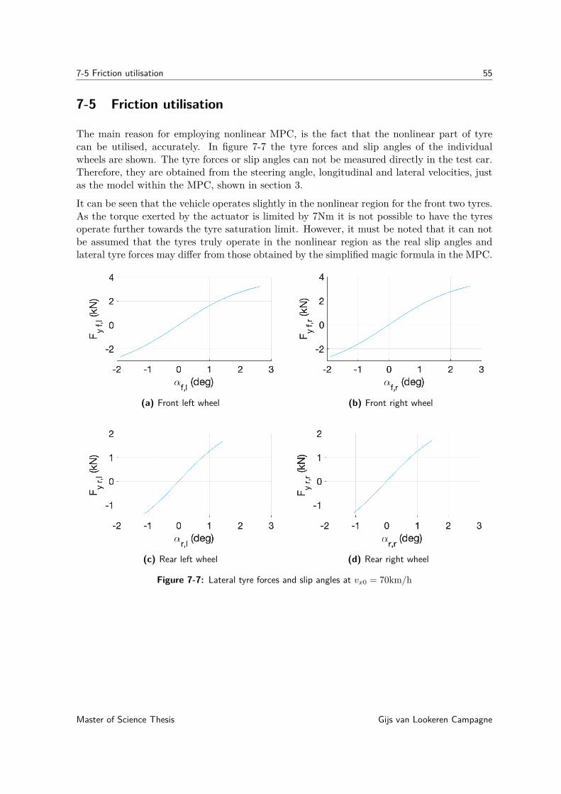
7-5 Friction utilisation 55
7-5 Friction utilisation
The main reason for employing nonlinear MPC, is the fact that the nonlinear part of tyrecan be utilised, accurately. In figure 7-7 the tyre forces and slip angles of the individualwheels are shown. The tyre forces or slip angles can not be measured directly in the test car.Therefore, they are obtained from the steering angle, longitudinal and lateral velocities, justas the model within the MPC, shown in section 3.
It can be seen that the vehicle operates slightly in the nonlinear region for the front two tyres.As the torque exerted by the actuator is limited by 7Nm it is not possible to have the tyresoperate further towards the tyre saturation limit. However, it must be noted that it can notbe assumed that the tyres truly operate in the nonlinear region as the real slip angles andlateral tyre forces may differ from those obtained by the simplified magic formula in the MPC.
(a) Front left wheel (b) Front right wheel
(c) Rear left wheel (d) Rear right wheel
Figure 7-7: Lateral tyre forces and slip angles at vx0 = 70km/h
Master of Science Thesis Gijs van Lookeren Campagne
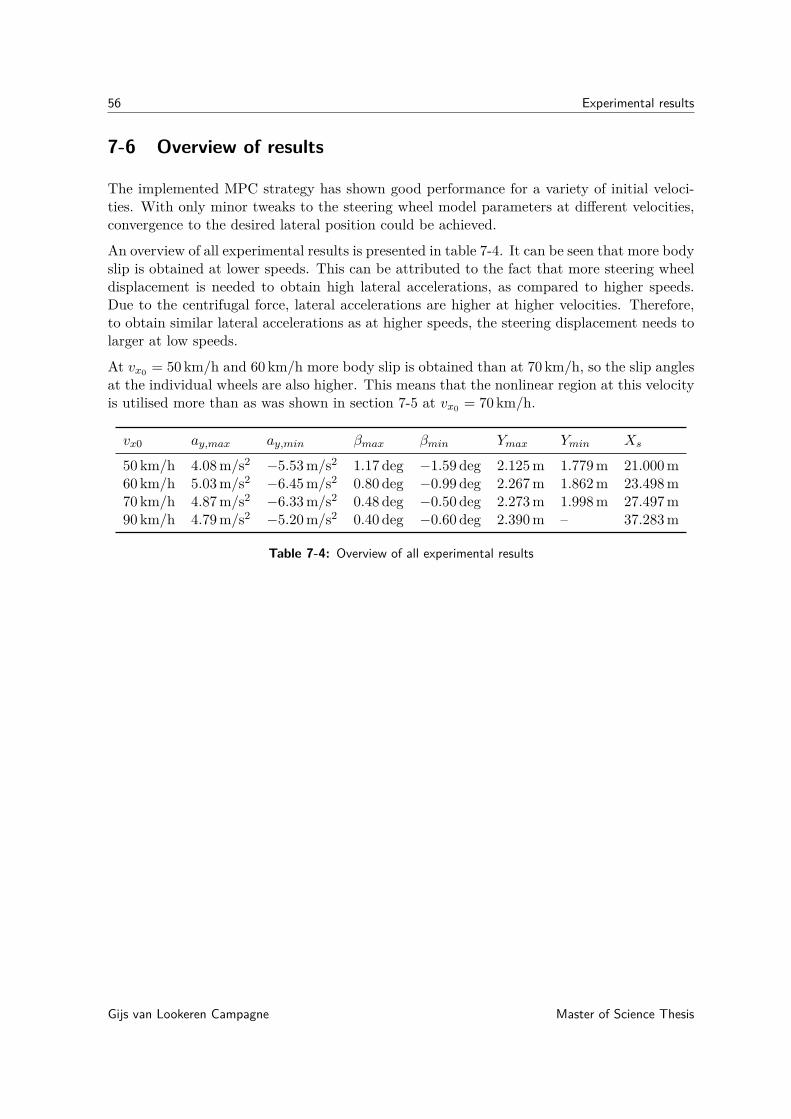
56 Experimental results
7-6 Overview of results
The implemented MPC strategy has shown good performance for a variety of initial veloci-ties. With only minor tweaks to the steering wheel model parameters at different velocities,convergence to the desired lateral position could be achieved.
An overview of all experimental results is presented in table 7-4. It can be seen that more bodyslip is obtained at lower speeds. This can be attributed to the fact that more steering wheeldisplacement is needed to obtain high lateral accelerations, as compared to higher speeds.Due to the centrifugal force, lateral accelerations are higher at higher velocities. Therefore,to obtain similar lateral accelerations as at higher speeds, the steering displacement needs tolarger at low speeds.
At vx0 = 50 km/h and 60 km/h more body slip is obtained than at 70 km/h, so the slip anglesat the individual wheels are also higher. This means that the nonlinear region at this velocityis utilised more than as was shown in section 7-5 at vx0 = 70 km/h.
vx0 ay,max ay,min βmax βmin Ymax Ymin Xs
50 km/h 4.08 m/s2 −5.53 m/s2 1.17 deg −1.59 deg 2.125 m 1.779 m 21.000 m60 km/h 5.03 m/s2 −6.45 m/s2 0.80 deg −0.99 deg 2.267 m 1.862 m 23.498 m70 km/h 4.87 m/s2 −6.33 m/s2 0.48 deg −0.50 deg 2.273 m 1.998 m 27.497 m90 km/h 4.79 m/s2 −5.20 m/s2 0.40 deg −0.60 deg 2.390 m – 37.283 m
Table 7-4: Overview of all experimental results
Gijs van Lookeren Campagne Master of Science Thesis

Chapter 8
Conclusion
In this thesis a real-time Nonlinear Model Predictive Control (NMPC) strategy was developedthat was able to carry out an aggressive evasive manoeuvre successfully. It was shown thatthe NMPC problem could be solved efficiently by regarding two state-of-the-art NonlinearProgramme (NLP) solvers.
Even though some simplifications were made in terms of vehicle and tyre models, good per-formance was obtained. This goes to show that the proposed MPC scheme is a robust methodand a promising prospect for limit handling safety systems. By employing even more accuratevehicle models, performance is likely to increase even further. This will become more feasibleas the processing power of Electronic Control Unit (ECU)s increases.
Compared to previous research, low sampling times were achieved for aggressive manoeuvres.In simulation, lateral accelerations up to 8.46 m/s2 were achieved. With limited actuation ofthe steering wheel, lateral accelerations up to 6.45 m/s2 were obtained for experimental testsin a test vehicle. In both cases, reasonable overshoots were obtained, while maintaining ashort longitudinal distance travelled. Moreover, it was shown that the nonlinear region ofthe tyre was utilised, which was the main motivation for implementing NMPC. A samplingfrequency of 25 Hz was accomplished on the embedded system in the test vehicle.
This thesis has shown that the proposed MPC strategy is able to handle model mismatchesand measurement inaccuracies well. Furthermore, the computational complexity that hasalways been an issue with NMPC has not shown to be problematic for real-time execution. Itcan be concluded that a mature MPC strategy on ECUs may very well be a feasible solutionfor future limit handling applications.
All in all, it can be concluded that Sequential Quadratic Programming (SQP) generallyperforms better for smaller constrained problems, whereas an Interior-Point Method (IPM)is more suited for larger unconstrained problems.
Master of Science Thesis Gijs van Lookeren Campagne
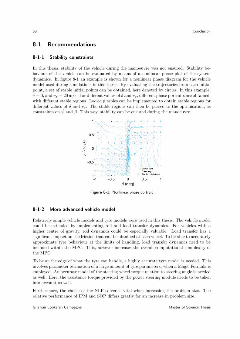
58 Conclusion
8-1 Recommendations
8-1-1 Stability constraints
In this thesis, stability of the vehicle during the manoeuvre was not ensured. Stability be-haviour of the vehicle can be evaluated by means of a nonlinear phase plot of the systemdynamics. In figure 8-1 an example is shown for a nonlinear phase diagram for the vehiclemodel used during simulations in this thesis. By evaluating the trajectories from each initialpoint, a set of stable initial points can be obtained, here denoted by circles. In this example,δ = 0, and vx = 20 m/s. For different values of δ and vx, different phase portraits are obtained,with different stable regions. Look-up tables can be implemented to obtain stable regions fordifferent values of δ and vx. The stable regions can then be passed to the optimisation, asconstraints on ψ and β. This way, stability can be ensured during the manoeuvre.
Figure 8-1: Nonlinear phase portrait
8-1-2 More advanced vehicle model
Relatively simple vehicle models and tyre models were used in this thesis. The vehicle modelcould be extended by implementing roll and load transfer dynamics. For vehicles with ahigher centre of gravity, roll dynamics could be especially valuable. Load transfer has asignificant impact on the friction that can be obtained at each wheel. To be able to accuratelyapproximate tyre behaviour at the limits of handling, load transfer dynamics need to beincluded within the MPC. This, however increases the overall computational complexity ofthe MPC.
To be at the edge of what the tyre can handle, a highly accurate tyre model is needed. Thisinvolves parameter estimation of a large amount of tyre parameters, when a Magic Formula isemployed. An accurate model of the steering wheel torque relation to steering angle is neededas well. Here, the assistance torque provided by the power steering module needs to be takeninto account as well.
Furthermore, the choice of the NLP solver is vital when increasing the problem size. Therelative performance of IPM and SQP differs greatly for an increase in problem size.
Gijs van Lookeren Campagne Master of Science Thesis
8-1 Recommendations 59
8-1-3 Implementation with additional driver applied torque
MPC and human driver behaviour are very analogous to each other. Human drivers do notonly take into account current time steps, but also future time steps. At the same time,human drivers may plan to carry out a manoeuvre that results in a loss of stability. Similarto an MPC problem, this can be regarded as a an infeasible manoeuvre.
The predictive nature of MPC may very well be helpful in critical situations where drivershave trouble finding an optimal solution to avoid a crash. The MPC can be used to assessthe risk of different situations and take measures in time. Depending of the the situation,driver intervention or assistance can be applied, just as current Evasive Manoeuvre AssistanceFunction (EMA) functions do. The advantage of MPC is that the driver can be assisted atan earlier stage, which can be crucial in near-collision situations.
8-1-4 Longitudinal inputs on an experimental setup
The combined steering and braking scenario is not tested on an experimental setup in thisthesis. It was found that SQP has more trouble handling a combined steering and brakingscenario than IPM does. Combined steering and braking might prove to be critical in near-collision situations. Not only braking could be implemented, but also positive torque on eachwheel, essentially yielding torque vectoring. This allows for quick and agile turns which couldbe very useful in critical situations.
8-1-5 Obstacle dependent cost function for collision avoidance
In this thesis a fixed baseline scenario was defined for a rear-collision situation. In reality,an infinite amount of near-collision scenarios could occur. For practical implementation, itwould be desired that the presence of obstacles is considered in the cost function. This way,an optimal trajectory can be determined, based on the position of different obstacles.
8-1-6 Experimental tests with higher steering wheel torque limits
Along with the transition to autonomous driving, power steering modules in vehicles will beable to provide higher steering wheel torques. This means that the actuator limits are sethigher than 7 Nm, allowing for more aggressive manoeuvres and the ability to truly utilisethe nonlinear part of the tyre in limit handling scenarios.
8-1-7 Embedded implementation of IPM
For larger sized problems, IPM solved by IPOPT becomes a more attractive approach. Thecommercial ForcesPro packages allows for self contained C code generation that can be de-ployed on embedded systems, using IPM. To extend the MPC scheme of this thesis toproblems that involve more advance vehicle models, a C coded IPM solver may prove to bea promising solution for an embedded system within a vehicle.
Master of Science Thesis Gijs van Lookeren Campagne
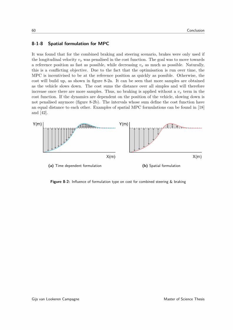
60 Conclusion
8-1-8 Spatial formulation for MPC
It was found that for the combined braking and steering scenario, brakes were only used ifthe longitudinal velocity vx was penalised in the cost function. The goal was to move towardsa reference position as fast as possible, while decreasing vx as much as possible. Naturally,this is a conflicting objective. Due to the fact that the optimisation is run over time, theMPC is incentivised to be at the reference position as quickly as possible. Otherwise, thecost will build up, as shown in figure 8-2a. It can be seen that more samples are obtainedas the vehicle slows down. The cost sums the distance over all simples and will thereforeincrease once there are more samples. Thus, no braking is applied without a vx term in thecost function. If the dynamics are dependent on the position of the vehicle, slowing down isnot penalised anymore (figure 8-2b). The intervals whose sum define the cost function havean equal distance to each other. Examples of spatial MPC formulations can be found in [18]and [42].
(a) Time dependent formulation (b) Spatial formulation
Figure 8-2: Influence of formulation type on cost for combined steering & braking
Gijs van Lookeren Campagne Master of Science Thesis

Appendix A
Simulation results
A-1 SQP & IPM (steering only) compared at computational limits
In sections 6-1 and 6-2 the steering only scenario was executed by means of both SequentialQuadratic Programming (SQP) and the Interior-Point Method (IPM). It was found that SQPresulted in significantly shorter computation times. To directly compare two methods thattake around 0.15 s (IPM) and 1.5·10−3s (SQP) would be unfair. Therefore, in this comparisonboth methods are tuned such that they run at the limits of what the computation time allowsfor.
A-1-1 SQP & IPM (steering only) formulation
The cost functions used in this chapter are listed below. The cost function for IPM remainsthe same cost function used for the steering only scenario in section 6-1.
JIPM =N∑k=1
2(Y (t+ k)− Yr(t+ k))2 + u(t+ k)2 (A-1)
Due to the fact that the Model Predictive Control (MPC) time parameters (table A-1) forSQP are considerably different from those used in section 6-2, a different cost function is usedfor SQP:
JSQP = 106(Y (N)− Yr(N))2 +N∑k=1
5 · 10−6(Y (t+ k)− Yr(t+ k))2 (A-2)
The MPC parameters for IPM and SQP found in table A-1 were found to match each otherin terms of performance. The computation times for both these tunings in simulation werefound to be just below the sampling time to ensure that both methods are close the limitsof the processor’s real-time capabilities. The sampling time for IPM is decreased to 0.1s to
Master of Science Thesis Gijs van Lookeren Campagne
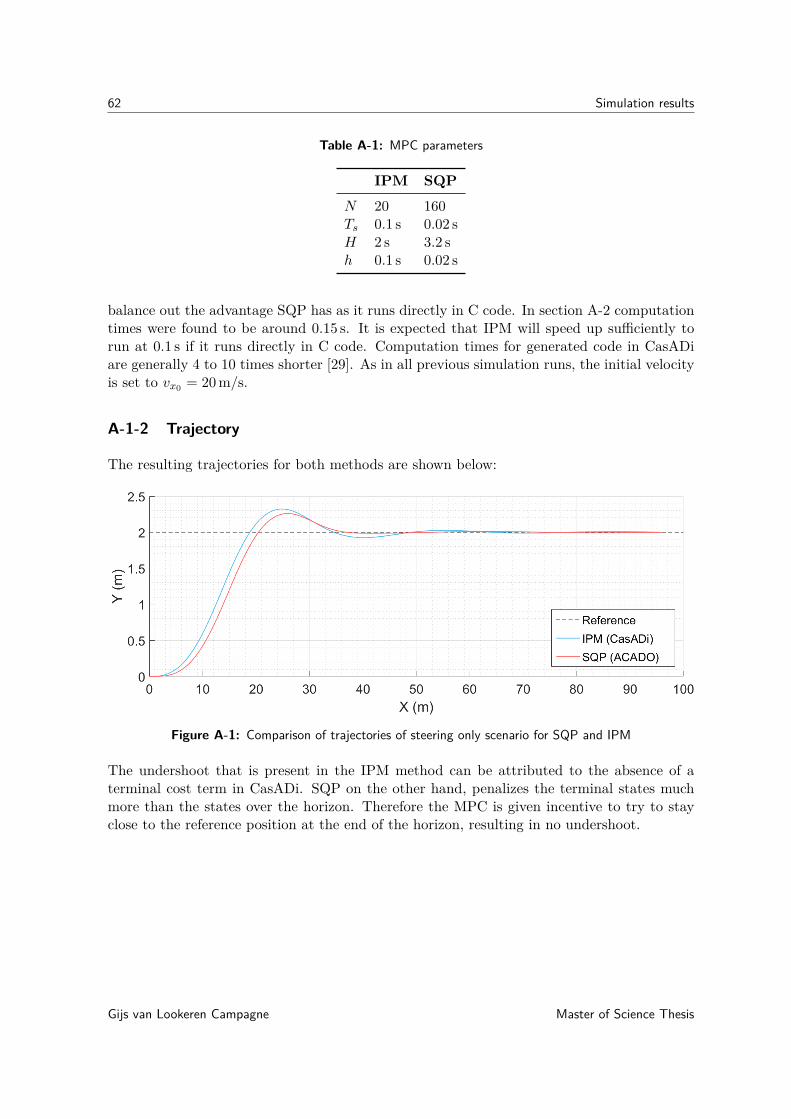
62 Simulation results
Table A-1: MPC parameters
IPM SQPN 20 160Ts 0.1 s 0.02 sH 2 s 3.2 sh 0.1 s 0.02 s
balance out the advantage SQP has as it runs directly in C code. In section A-2 computationtimes were found to be around 0.15 s. It is expected that IPM will speed up sufficiently torun at 0.1 s if it runs directly in C code. Computation times for generated code in CasADiare generally 4 to 10 times shorter [29]. As in all previous simulation runs, the initial velocityis set to vx0 = 20 m/s.
A-1-2 Trajectory
The resulting trajectories for both methods are shown below:
Figure A-1: Comparison of trajectories of steering only scenario for SQP and IPM
The undershoot that is present in the IPM method can be attributed to the absence of aterminal cost term in CasADi. SQP on the other hand, penalizes the terminal states muchmore than the states over the horizon. Therefore the MPC is given incentive to try to stayclose to the reference position at the end of the horizon, resulting in no undershoot.
Gijs van Lookeren Campagne Master of Science Thesis

A-1 SQP & IPM (steering only) compared at computational limits 63
A-1-3 Notable results
The remaining measurements are shown in figure A-2. It can be seen that SQP and IPMshow nearly identical behaviour for these tunings. The identical behaviour helps to validatethat both methods do indeed yield an optimal trajectory for the posed problem.
Compared to the previous tuning for IPM in section A-2, a much smoother response is ob-tained by decreasing the sampling time to 0.1s. It does make for a less aggressive manoeuvrewith a considerably lower steering angle and body slip.
(a) Steering angle (b) Body slip angle
(c) Lateral acceleration (d) Longitudinal velocity
Figure A-2: Comparison of results for SQP and IPM
Master of Science Thesis Gijs van Lookeren Campagne

64 Simulation results
A-1-4 Computation times
The computation times for both methods are shown below. The mean computation timestc,mean for IPM and SQP are 0.147 s and 0.0096 s, respectively.
(a) Computation times (IPM) (b) Computation times (SQP)
Figure A-3: Computation times for SQP and IPM
Gijs van Lookeren Campagne Master of Science Thesis

A-1 SQP & IPM (steering only) compared at computational limits 65
A-1-5 Friction utilisation
The reason for employing Nonlinear Model Predictive Control (NMPC) was to be able toutilise the nonlinear region of the tyre. In this section it is assessed whether the nonlinearpart of the tyre is used indeed. The tyre model within the MPC is a simplified Magic Formula,as shown in section 3. In the vehicle model that CarMaker uses, a full 5.2 Magic Formula[43] is used. As there is a mismatch between the model within the MPC and the highlyrealistic CarMaker vehicle model, both models yield different slip angles and tyre forces. Inthis section, the utilised friction for both the model within the MPC as well as simulations inCarMaker is considered.
In figure A-3 the measured slip angles are shown for the rear left wheel in CarMaker. Theyare plotted against the lateral tyre forces, using the simplified Magic Formula used in theMPC, as shown in equation (3-10).
This figure displays to what extent the nonlinear part of the tyre is being utilised. For bothSQP and IPM the nonlinear part of tyre is clearly utilised. The maximum slip angles for bothmethods are still somewhat off the tyre saturation point. However, it can not be assumedthat larger slip angles will result in better performance. The MPC runs an optimisationover time. By increasing the slip on the wheels, more longitudinal velocity is lost whileexecuting the manoeuvre. This results in the car taking more time to reach to its referenceposition compared to a situation with less slip. Therefore, the MPC is more likely to opt fora manoeuvre with slightly lower slip angles.
(a) SQP (b) IPM
Figure A-4: Friction utilisation of rear left wheel for SQP and IPM
The utilised friction for both methods is very similar. The maximum slip angle for IPM isslightly higher than for SQP. SQP is more present at the lower slip angles whereas IPMutilises the higher slip angles slightly more. The slip angle frequency distribution for bothmethods is shown in figure A-5. It can be seen that IPM utilises large slip angles slightlymore than SQP.
Master of Science Thesis Gijs van Lookeren Campagne

66 Simulation results
Figure A-5: Obtained slip angles for SQP and IPM
Gijs van Lookeren Campagne Master of Science Thesis
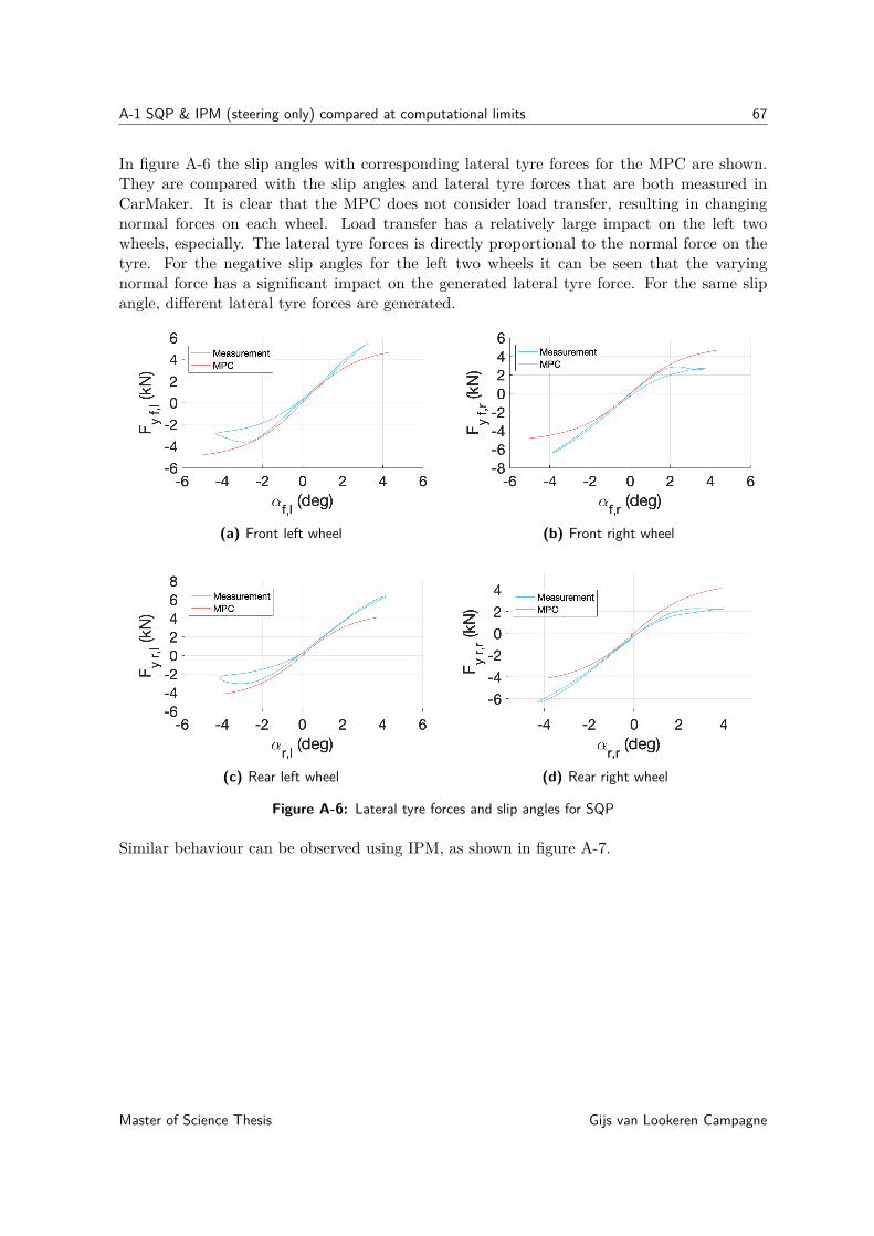
A-1 SQP & IPM (steering only) compared at computational limits 67
In figure A-6 the slip angles with corresponding lateral tyre forces for the MPC are shown.They are compared with the slip angles and lateral tyre forces that are both measured inCarMaker. It is clear that the MPC does not consider load transfer, resulting in changingnormal forces on each wheel. Load transfer has a relatively large impact on the left twowheels, especially. The lateral tyre forces is directly proportional to the normal force on thetyre. For the negative slip angles for the left two wheels it can be seen that the varyingnormal force has a significant impact on the generated lateral tyre force. For the same slipangle, different lateral tyre forces are generated.
(a) Front left wheel (b) Front right wheel
(c) Rear left wheel (d) Rear right wheel
Figure A-6: Lateral tyre forces and slip angles for SQP
Similar behaviour can be observed using IPM, as shown in figure A-7.
Master of Science Thesis Gijs van Lookeren Campagne

68 Simulation results
(a) Front left wheel (b) Front right wheel
(c) Rear left wheel (d) Rear right wheel
Figure A-7: Lateral tyre forces and slip angles for IPM
Gijs van Lookeren Campagne Master of Science Thesis
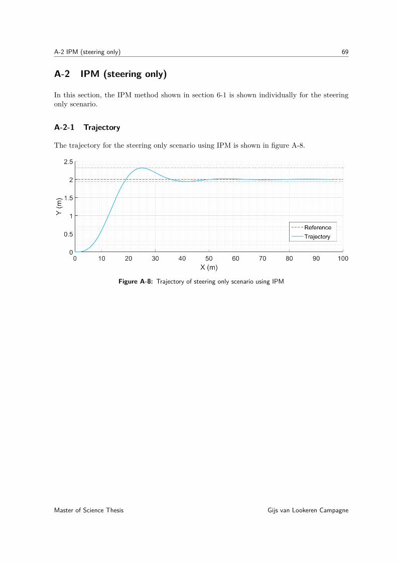
A-2 IPM (steering only) 69
A-2 IPM (steering only)
In this section, the IPM method shown in section 6-1 is shown individually for the steeringonly scenario.
A-2-1 Trajectory
The trajectory for the steering only scenario using IPM is shown in figure A-8.
Figure A-8: Trajectory of steering only scenario using IPM
Master of Science Thesis Gijs van Lookeren Campagne
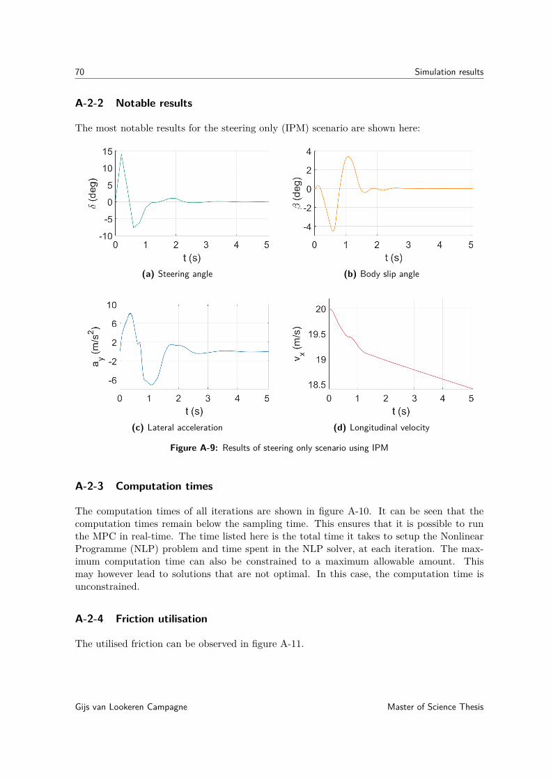
70 Simulation results
A-2-2 Notable results
The most notable results for the steering only (IPM) scenario are shown here:
(a) Steering angle (b) Body slip angle
(c) Lateral acceleration (d) Longitudinal velocity
Figure A-9: Results of steering only scenario using IPM
A-2-3 Computation times
The computation times of all iterations are shown in figure A-10. It can be seen that thecomputation times remain below the sampling time. This ensures that it is possible to runthe MPC in real-time. The time listed here is the total time it takes to setup the NonlinearProgramme (NLP) problem and time spent in the NLP solver, at each iteration. The max-imum computation time can also be constrained to a maximum allowable amount. Thismay however lead to solutions that are not optimal. In this case, the computation time isunconstrained.
A-2-4 Friction utilisation
The utilised friction can be observed in figure A-11.
Gijs van Lookeren Campagne Master of Science Thesis
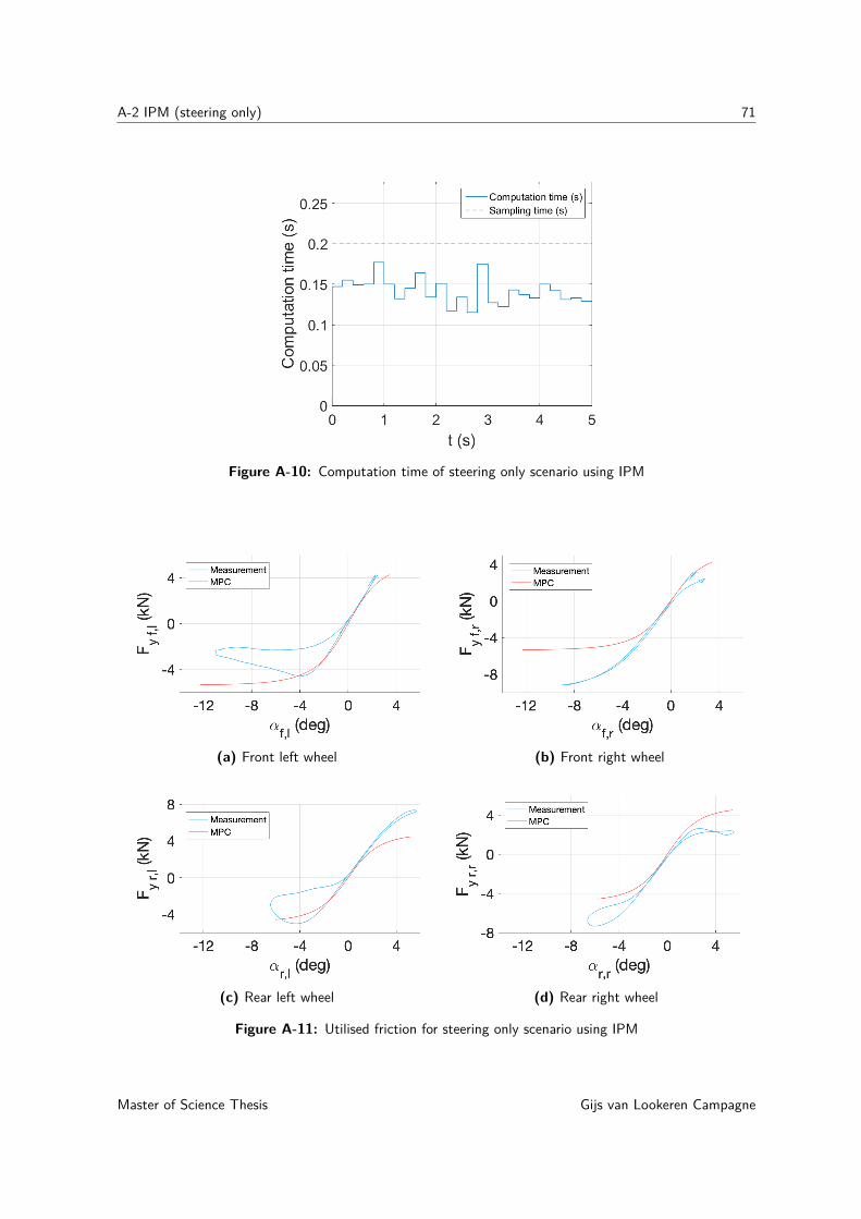
A-2 IPM (steering only) 71
Figure A-10: Computation time of steering only scenario using IPM
(a) Front left wheel (b) Front right wheel
(c) Rear left wheel (d) Rear right wheel
Figure A-11: Utilised friction for steering only scenario using IPM
Master of Science Thesis Gijs van Lookeren Campagne
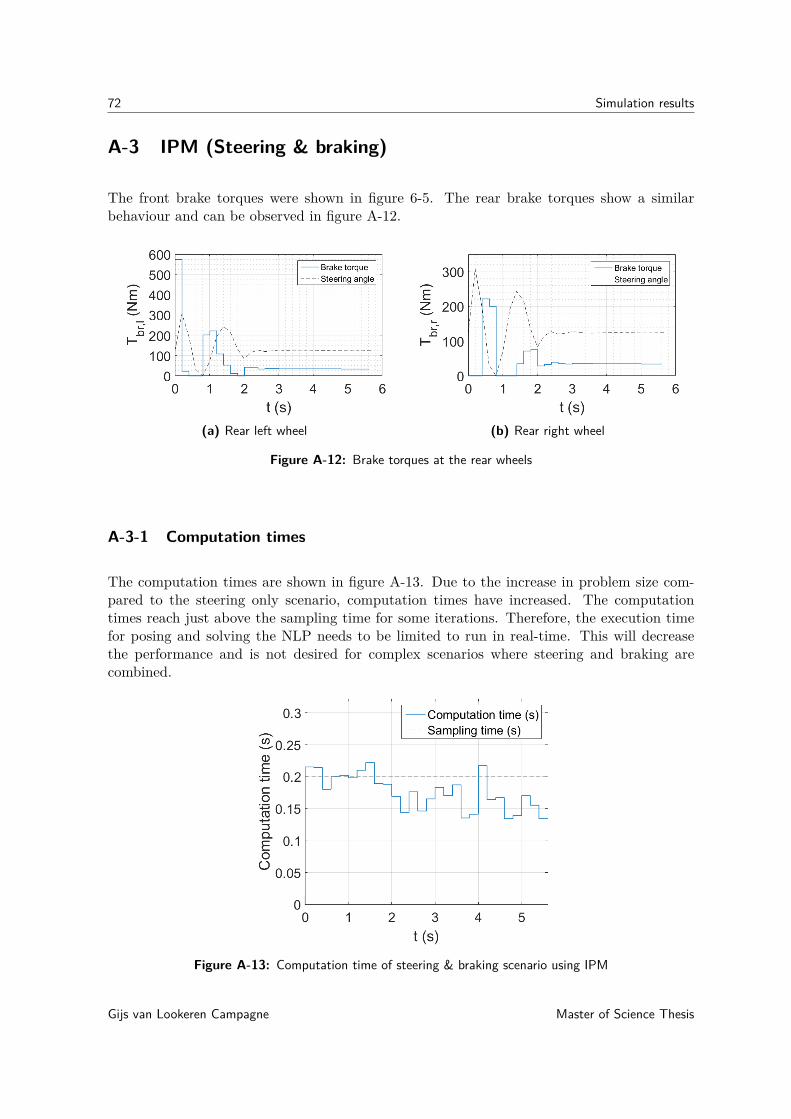
72 Simulation results
A-3 IPM (Steering & braking)
The front brake torques were shown in figure 6-5. The rear brake torques show a similarbehaviour and can be observed in figure A-12.
(a) Rear left wheel (b) Rear right wheel
Figure A-12: Brake torques at the rear wheels
A-3-1 Computation times
The computation times are shown in figure A-13. Due to the increase in problem size com-pared to the steering only scenario, computation times have increased. The computationtimes reach just above the sampling time for some iterations. Therefore, the execution timefor posing and solving the NLP needs to be limited to run in real-time. This will decreasethe performance and is not desired for complex scenarios where steering and braking arecombined.
Figure A-13: Computation time of steering & braking scenario using IPM
Gijs van Lookeren Campagne Master of Science Thesis

A-3 IPM (Steering & braking) 73
A-3-2 Friction utilisation
The utilised friction for the steering and braking scenario (IPM) can be seen in figure A-14.The simplified Magic Formula does not incorporate any combined slip. Longitudinal andlateral slip influence each other, so a solely lateral tyre model lacks accuracy for a combinedslip scenario. More advanced tyre models incorporate combined slip behaviour. Along withthe previously explained lack of load transfer, a significant model mismatch is present here.
(a) Front left wheel (b) Front right wheel
(c) Rear left wheel (d) Rear right wheel
Figure A-14: Utilised friction for steering & braking scenario using IPM
Master of Science Thesis Gijs van Lookeren Campagne

74 Simulation results
A-4 SQP (steering only)
A-4-1 Computation times
The computation times for SQP are shown in figure A-15. Clearly, computation times arewell below the sampling time (0.04s). ACADO and SQP are known to perform efficiently forsmaller sized problems, such as is the case in this scenario.
Figure A-15: Computation time of steering scenario using SQP
Gijs van Lookeren Campagne Master of Science Thesis
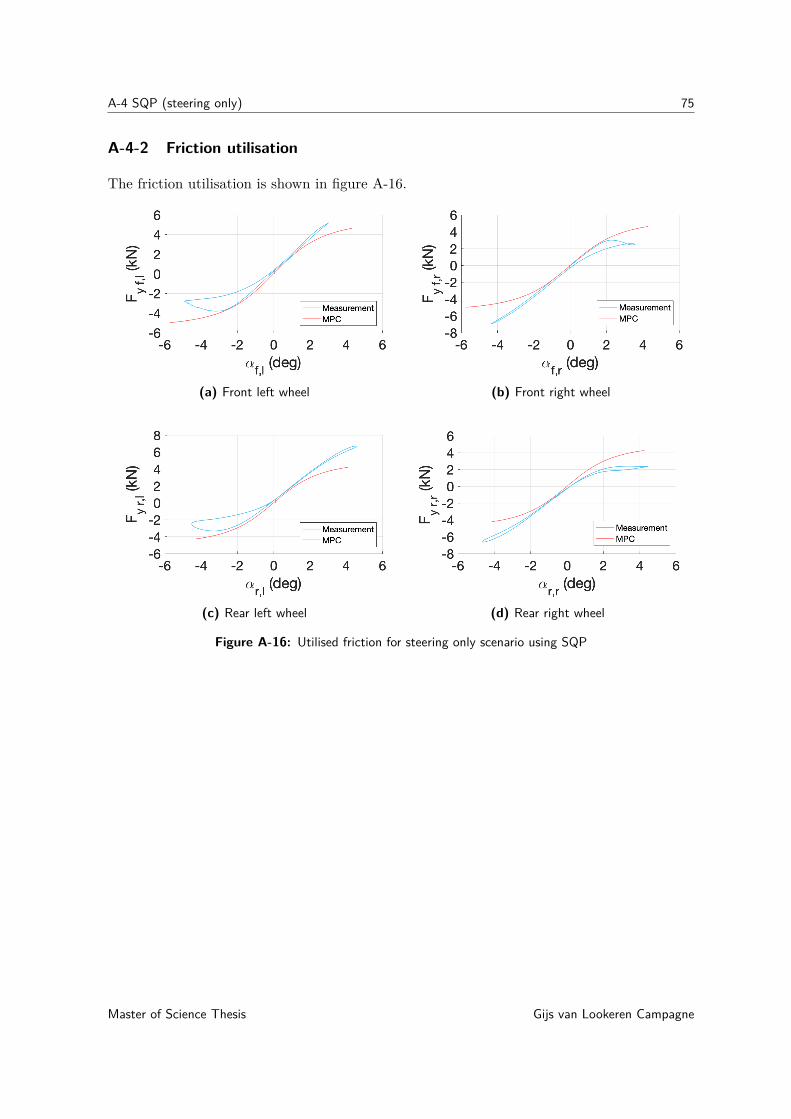
A-4 SQP (steering only) 75
A-4-2 Friction utilisation
The friction utilisation is shown in figure A-16.
(a) Front left wheel (b) Front right wheel
(c) Rear left wheel (d) Rear right wheel
Figure A-16: Utilised friction for steering only scenario using SQP
Master of Science Thesis Gijs van Lookeren Campagne

76 Simulation results
A-5 Scalability to different scenarios
In this section a comparison is made between the use of different reference positions in thecost function and the influence of different initial velocities on the performance of the MPC.The aim here is to see how well the MPC scales when a slightly different problem is posed.It must be noted that for each objective the MPC can be retuned. However, in real-lifedriving scenarios there are are an infinite amount of possible scenarios and it is cumbersometo tune for each different scenario. Therefore, in this section the MPC formulation remains thesame throughout the different scenarios so that it can be observed how well the MPC scaleswith different problems. Of course, scalability may differ among different cost functions. Anaggressively tuned cost function is more likely to fail when it is applied to a different problem.The results in this section are aimed to reflect the general scalability that was observed fordifferent tunings of both SQP and IPM during this thesis. The cost functions remain thesame as in (6-2) and (6-5).
In the reference comparisons only the global reference position Yr is changed. The weightsin the cost function remain the same. In the initial velocity comparison the cost functionremains completely the same and only the initial velocity is adjusted.
A-5-1 Comparison of multiple references
In this section different reference positions are compared for both NLP methods.
SQP
Figure A-17: Scalability of reference position using SQP (N = 40)
In figure A-17 the same MPC is used as as in section 6-2-1. It can be seen that the MPCdoes not scale well for different reference positions as it fails to track Yr = 1m and Yr = 3mwith the same performance as Yr = 2m, which it was tuned for. There is a large overshootpresent for Yr = 3m and an offset for Yr = 1m. However when the horizon is increased toN = 80, SQP scales much better for different reference positions, as can be seen in A-18.
Gijs van Lookeren Campagne Master of Science Thesis

A-5 Scalability to different scenarios 77
Figure A-18: Scalability of reference position using SQP (N = 80)
IPM
Figure A-19: Scalability of reference position using IPM
IPM, on the other hand, scales very well with different reference positions for the baselinetuning found in section A-2. The overshoot scales proportional to the given reference and itis possible to track Yr = 4 m with ease.
Master of Science Thesis Gijs van Lookeren Campagne

78 Simulation results
A-5-2 Comparison of multiple initial velocities
In order to show the versatility of the proposed MPC scheme, the trajectories for differentinitial velocities are shown in this section.
IPM
Figure A-20: Scalability of initial velocity using IPM
IPM is able to scale well with different inital velocities as well. As seen before, IPM reachesthe 2m safe-zone slightly faster than SQP.
SQP
Figure A-21: Scalability of initial velocity using SQP
SQP is able to track the reference at different initial velocities without the need for increasingthe amount of control intervals.
Gijs van Lookeren Campagne Master of Science Thesis

A-6 Horizon comparison 79
A-6 Horizon comparison
The time horizons considered in the previous sections were kept constant at 2 s and 1.6 s forIPM and SQP, respectively. In this section, both time horizons H are increased twofold.
A-6-1 IPM
Figure A-22: Comparison of different horizons using IPM
It can be seen that an increase in the horizon makes for a slightly less aggressive manoeuvre.This can be attributed to the fact that for a short horizon only the first part of the manoeuvreis considered. For a longer horizon, the weight of the first part of the manoeuvre is relativelylower, resulting in a more relaxed manoeuvre.
A-6-2 SQP
Figure A-23: Comparison of different horizons using SQP
Master of Science Thesis Gijs van Lookeren Campagne
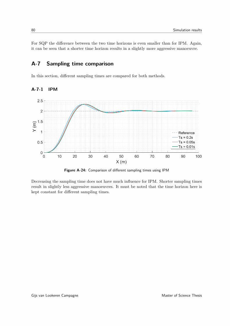
80 Simulation results
For SQP the difference between the two time horizons is even smaller than for IPM. Again,it can be seen that a shorter time horizon results in a slightly more aggressive manoeuvre.
A-7 Sampling time comparison
In this section, different sampling times are compared for both methods.
A-7-1 IPM
Figure A-24: Comparison of different sampling times using IPM
Decreasing the sampling time does not have much influence for IPM. Shorter sampling timesresult in slightly less aggressive manoeuvres. It must be noted that the time horizon here iskept constant for different sampling times.
Gijs van Lookeren Campagne Master of Science Thesis

A-7 Sampling time comparison 81
A-7-2 SQP
Figure A-25: Comparison of different sampling times using SQP
It must be noted that decreasing the sampling time to 0.01 s did not result in convergence tothe reference position. This can be attributed to the fact that the amount of control intervalsremains unchanged for the different sampling times shown here, resulting in a very short timehorizon. When N = 40, a sampling time of 0.04 s results in H = 1.6 s, whereas Ts = 0.01 sresults in H = 0.4 s. If the time horizon is kept constant as was done using IPM, it is likelythat behaviour for the different sampling times is similar as for IPM. The MPC is not able toconverge to the reference for such short time horizons. It can be concluded that a balancedtrade-off needs to be made in regard to Ts and N .
Master of Science Thesis Gijs van Lookeren Campagne

82 Simulation results
Gijs van Lookeren Campagne Master of Science Thesis
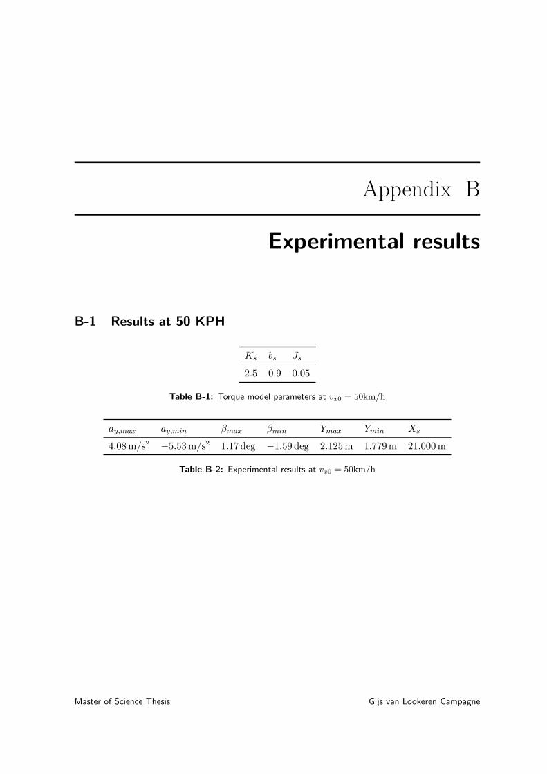
Appendix B
Experimental results
B-1 Results at 50 KPH
Ks bs Js
2.5 0.9 0.05
Table B-1: Torque model parameters at vx0 = 50km/h
ay,max ay,min βmax βmin Ymax Ymin Xs
4.08 m/s2 −5.53 m/s2 1.17 deg −1.59 deg 2.125 m 1.779 m 21.000 m
Table B-2: Experimental results at vx0 = 50km/h
Master of Science Thesis Gijs van Lookeren Campagne

84 Experimental results
Figure B-1: Trajectory of experimental test at vx0 = 50km/h
(a) Steering angle (b) Body slip angle
(c) Lateral acceleration (d) Longitudinal velocity
Figure B-2: Results of experimental test at vx0 = 50km/h
Gijs van Lookeren Campagne Master of Science Thesis

B-2 Results at 60 KPH 85
Figure B-3: Requested torque and steering wheel angle at vx0 = 50km/h
B-2 Results at 60 KPH
Ks bs Js
3.5 0.9 0.05
Table B-3: Torque model parameters at vx0 = 60km/h
vx0 ay,max ay,min βmax βmin Ymax Ymin Xs
5.03 m/s2 −6.45 m/s2 0.80 deg −0.99 deg 2.267 m 1.862 m 23.498 m
Table B-4: Experimental results at vx0 = 60km/h
Master of Science Thesis Gijs van Lookeren Campagne
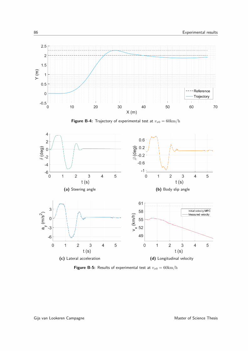
86 Experimental results
Figure B-4: Trajectory of experimental test at vx0 = 60km/h
(a) Steering angle (b) Body slip angle
(c) Lateral acceleration (d) Longitudinal velocity
Figure B-5: Results of experimental test at vx0 = 60km/h
Gijs van Lookeren Campagne Master of Science Thesis

B-3 Results at 90 KPH 87
Figure B-6: Requested torque and steering wheel angle at vx0 = 60km/h
B-3 Results at 90 KPH
Ks bs Js
4.5 0.9 0.05
Table B-5: Torque model parameters at vx0 = 90km/h
ay,max ay,min βmax βmin Ymax Ymin Xs
4.79 m/s2 −5.20 m/s2 0.40 deg −0.60 deg 2.39 m – 37.283 m
Table B-6: Experimental results at vx0 = 90km/h
Master of Science Thesis Gijs van Lookeren Campagne
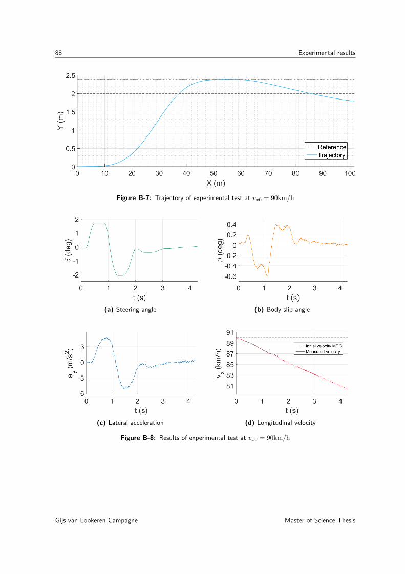
88 Experimental results
Figure B-7: Trajectory of experimental test at vx0 = 90km/h
(a) Steering angle (b) Body slip angle
(c) Lateral acceleration (d) Longitudinal velocity
Figure B-8: Results of experimental test at vx0 = 90km/h
Gijs van Lookeren Campagne Master of Science Thesis
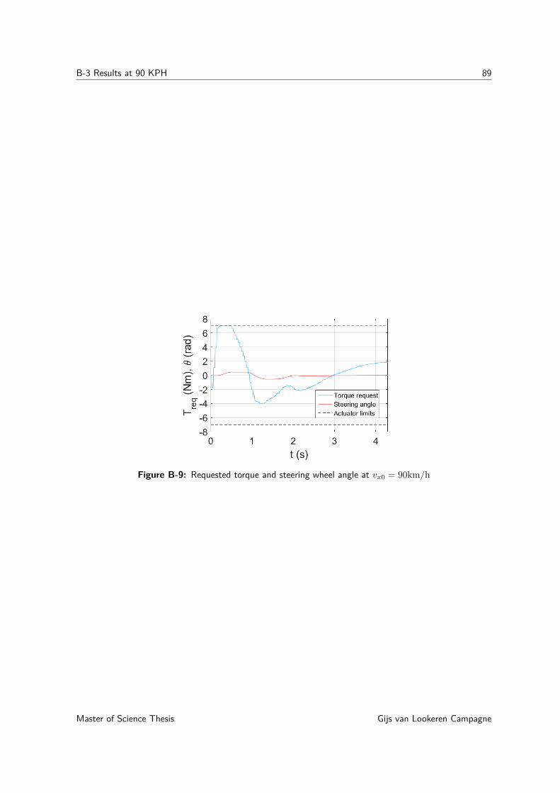
B-3 Results at 90 KPH 89
Figure B-9: Requested torque and steering wheel angle at vx0 = 90km/h
Master of Science Thesis Gijs van Lookeren Campagne

90 Experimental results
B-4 Comparison between driver, simulation and experiment
Figure B-10: Trajectory comparison for driver, simulation and experiment
While carrying out experimental tests, driver data was logged as well. A comparison of driver,simulation and experimental data can be seen in figures B-10 and B-11. No cones or any otherpositioning marks were used when the driver carried out the manoeuvre. The driver had noreference as to what was the actual lateral displacement. Therefore, the lateral displacementis slightly larger and it is hard to draw a fair comparison. It can be seen that a driver isable to initiate a more aggressive manoeuvre. The lateral displacement is larger for the samedistance travelled. For a higher torque actuator limit, the Model Predictive Control (MPC)initiated manoeuvre would come closer to the aggressiveness of the driver.
Figure B-11: Torque request and steering angle comparison for driver, simulation and experiment
In figure B-11, the steering wheel torque (experiment), torsion bar torque (driver) and steeringangles are shown. For driver applied torque, only the torsion bar torque can be measured.The torque applied at the steering wheel is different from the torque measured at the torsionbar. This results in a lower measured torque magnitude for the torsion bar. However, theoverall pattern of applied torque is similar for the driver data and the experimental data.
Gijs van Lookeren Campagne Master of Science Thesis
Bibliography
[1] T. Dang, J. Desens, U. Franke, D. Gavrila, L. Schäfers, and W. Ziegler, “Steering andEvasion Assist,” in Handbook of Intelligent Vehicles, vol. 1-2, pp. 1–1599, 2012.
[2] R. Bentley, Speed secrets: professional race driving techniques. 1998.
[3] “Model Predictive Control - MPC technology from ABB - What is new.”
[4] B. Yi, Integrated Planning and Control for Collision Avoidance Systems. 2018.
[5] S. Singh, “Critical reasons for crashes investigated in the National Motor Vehicle CrashCausation Survey,” National Highway Traffic Safety Administration, no. February, pp. 1–2, 2015.
[6] D. Lechner and G. Malaterre, “Emergency Manuever Experimentation Using a DrivingSimulator,” Sae 910016, 1991.
[7] S. Singh, “Driver attributes and rear-end crash involvement propensity,” pp. 1–29, 2003.
[8] J. N. Dang, “Statistical Analysis of the Effectiveness of Electronic Stability Control(ESC) Systems Final Report,” NHTSA Report No. DOT HS, vol. 810, no. July, p. 794,2007.
[9] E. Camacho and C. Alba, Model predictive control. 2013.
[10] Bovag, “Mobiliteit in Cijfers Auto’s 2015/2016,” 2015.
[11] V. A. Laurense, J. Y. Goh, and J. C. Gerdes, “Path-tracking for autonomous vehicles atthe limit of friction,” Proceedings of the American Control Conference, pp. 5586–5591,2017.
[12] C. E. Beal and J. C. Gerdes, “Model predictive control for vehicle stabilization at thelimits of handling,” IEEE Transactions on Control Systems Technology, vol. 21, no. 4,pp. 1258–1269, 2013.
Master of Science Thesis Gijs van Lookeren Campagne

92 Bibliography
[13] A. Katriniok and D. Abel, “LTV-MPC approach for lateral vehicle guidance by frontsteering at the limits of vehicle dynamics,” Proceedings of the IEEE Conference on De-cision and Control, pp. 6828–6833, 2011.
[14] N. R. Kapania, J. Subosits, and J. Christian Gerdes, “A Sequential Two-Step Algo-rithm for Fast Generation of Vehicle Racing Trajectories,” Journal of Dynamic Systems,Measurement, and Control, vol. 138, no. 9, p. 091005, 2016.
[15] S. Heinrich, “Obstacle Avoidance with Safety Guarantees Feasibility of MPC-based Steer-ing Algorithms,” p. 95, 2015.
[16] S. J. Anderson, S. C. Peters, T. E. Pilutti, and K. Iagnemma, “Design and developmentof an optimal-control-based framework for trajectory planning, threat assessment, andsemi-autonomous control of passenger vehicles in hazard avoidance scenarios,” SpringerTracts in Advanced Robotics, vol. 70, no. STAR, pp. 39–54, 2011.
[17] A. Carvalho, Y. Gao, A. Gray, H. E. Tseng, and F. Borrelli, “Predictive control of anautonomous ground vehicle using an iterative linearization approach,” IEEE Conferenceon Intelligent Transportation Systems, Proceedings, ITSC, no. Itsc, pp. 2335–2340, 2013.
[18] S. M. Erlien, S. Fujita, and J. C. Gerdes, “Shared Steering Control Using Safe Envelopesfor Obstacle Avoidance and Vehicle Stability,” IEEE Transactions on Intelligent Trans-portation Systems, vol. 17, no. 2, pp. 441–451, 2016.
[19] J. Funke, M. Brown, S. M. Erlien, and J. C. Gerdes, “Collision Avoidance and Stabiliza-tion for Autonomous Vehicles in Emergency Scenarios,” IEEE Transactions on ControlSystems Technology, vol. 25, no. 4, pp. 1204–1216, 2017.
[20] Y. Gao, “Model Predictive Control for Autonomous and Semiautonomous Vehicles,”ProQuest Dissertations and Theses, 2014.
[21] J. V. Frasch, A. Gray, M. Zanon, H. J. Ferreau, S. Sager, F. Borrelli, and M. Diehl,“An auto-generated nonlinear MPC algorithm for real-time obstacle avoidance of groundvehicles,” Control Conference (ECC), 2013 European, pp. 4136–4141, 2013.
[22] A. Gray, Y. Gao, T. Lin, J. K. Hedrick, H. E. Tseng, and F. Borrelli, “Predictive controlfor agile semi-autonomous ground vehicles using motion primitives,” American ControlConference (ACC), 2012, pp. 4239–4244, 2012.
[23] P. Falcone, F. Borrelli, J. Asgari, H. E. Tseng, and D. Hrovat, “Predictive active steer-ing control for autonomous vehicle systems,” IEEE Transactions on Control SystemsTechnology, vol. 15, no. 3, pp. 566–580, 2007.
[24] H. B. P. . E. Bakker, “Experience with the magic formula tyre model,” Vehicle SystemDynamics, vol. 21, no. sup1, pp. 30–46, 1992.
[25] P. Falcone, H. Eric Tseng, F. Borrelli, J. Asgari, and D. Hrovat, “MPC-based yaw andlateral stabilisation via active front steering and braking,” in Vehicle System Dynamics,vol. 46, pp. 611–628, 2008.
[26] V. Cars, “Volvo Cars and NVIDIA deepen ties,” 2018.
Gijs van Lookeren Campagne Master of Science Thesis

93
[27] T. Shim, G. Adireddy, and H. Yuan, “Autonomous vehicle collision avoidance systemusing path planning and model-predictive-control-based active front steering and wheeltorque control,” Proceedings of the Institution of Mechanical Engineers, Part D: Journalof Automobile Engineering, vol. 226, no. 6, pp. 767–778, 2012.
[28] A. Wachter, On the implementation of an interior-point filter line-search algorithm forlarge-scale nonlinear programming. 2005.
[29] J. A. E. Andersson, J. Gillis, G. Horn, J. B. Rawlings, and M. Diehl, “CasADi: a softwareframework for nonlinear optimization and optimal control,” Mathematical ProgrammingComputation, 2018.
[30] H. J. Ferreau, C. Kirches, A. Potschka, H. G. Bock, and M. Diehl, “qpOASES: a para-metric active-set algorithm forÂăquadratic programming,” Mathematical ProgrammingComputation, vol. 6, no. 4, pp. 327–363, 2014.
[31] B. Houska, H. J. Ferreau, and M. Diehl, “Automatica An auto-generated real-time iter-ation algorithm for nonlinear MPC in the,” Automatica, vol. 47, no. 10, pp. 2279–2285,2011.
[32] J. Andersson, “Performance of Casadi vs. Acado for NMPC [Online forum comment],”2017.
[33] V. Leek, “An Optimal Control Toolbox for MATLAB Based on CasADi,” 2016.
[34] J. Andersson and M. Diehl, User Documentation for CasADi v2.2.0. 2015.
[35] H. Bock and K. Plitt, “A Multiple Shooting Algorithm for Direct Solution of OptimalControl Problems *,” IFAC Proceedings Volumes, vol. 17, no. 2, pp. 1603–1608, 1984.
[36] P. T. Boggs, W. J. Tolle, and J. W. Tolle, “Sequential Quadratic Programming,” ActaNumerica, vol. 4, no. November 2008, pp. 1–52, 1996.
[37] J. M. Maciejowski, “(Maciejowsky, 2000) - Predictive Control with Constraints,” 2002.
[38] M. Diehl, H. G. Bock, H. Diedam, P.-b. Wieber, M. Diehl, H. G. Bock, H. Diedam,P.-b. W. Fast, and D. Multiple, “Fast Direct Multiple Shooting Algorithms for OptimalRobot Control,” 2009.
[39] J. T. Betts, “Survey of Numerical Methods for Trajectory Optimization,” Journal ofGuidance, Control, and Dynamics, vol. 21, no. 2, pp. 193–207, 1998.
[40] D. Yang, T. J. Gordon, B. Jacobson, and M. Jonasson, “Quasi-linear optimal pathcontroller applied to post impact vehicle dynamics,” IEEE Transactions on IntelligentTransportation Systems, vol. 13, no. 4, pp. 1586–1598, 2012.
[41] D. I. Katzourakis, Driver Steering Support Interfaces Near the Vehicle’s Handling Limits.2012.
[42] Y. Gao, A. Gray, J. V. Frasch, T. Lin, E. Tseng, J. K. Hedrick, and F. Borrelli, “SpatialPredictive Control for Agile Semi-Autonomous Ground Vehicles,” Proceedings of the 11thInternational Symposium on Advanced Vehicle Control, vol. VD11, no. 2, pp. 1–6, 2012.
[43] H. B. Pacejka, Tyre characteristics and vehicle handling and stability. 2007.
Master of Science Thesis Gijs van Lookeren Campagne

94 Bibliography
Gijs van Lookeren Campagne Master of Science Thesis
Glossary
List of Acronyms
MPC Model Predictive Control
NMPC Nonlinear Model Predictive Control
PID Proportional-Integral-Derivative control
NLP Nonlinear Programme
QP Quadratic Programming
IPM Interior-Point Method
SQP Sequential Quadratic Programming
KKT Karush-Kuhn-Tucker Conditions
EMA Evasive Manoeuvre Assistance Function
IMU Inertial Measurement Unit
RTI Real-time Interface
ADAS Advanced Driver Assistance Systems
CAN Controller Area Network
ECU Electronic Control Unit
DSR Driver Steering Recommendation
ESC Electronic Stability Control
Master of Science Thesis Gijs van Lookeren Campagne
96 Glossary
List of Symbols
Bd Driveline damping coefficientH Time horizonh Control interval time stepIz Yaw moment of inertia of the vehicle C1
IdiWheel moment of inertia C2
m Mass of the vehicleN Horizonr Wheel radiusTbi
Brake torque at wheel C2
ur Reference control inputw Track widthxr Reference state vectorXs Longitudinal distance travelled to reach Y = 2 mωi Angular velocity of wheel C2
C0 Global coordinate frameC1 Local vehicle coordinate frameC2 Local wheel coordinate framelf Distance from centre of gravity to front axlelr Distance from centre of gravity to front axleαi Slip angle C2
x Longitudinal acceleration C1
y Lateral acceleration C1
δ Steering rate C1
ψ Yaw rate C1
x Longitudinal velocity C1
y Lateral velocity C1
κ Slip ratioFci Lateral tyre force C2
Fli Longitudinal tyre force C2
Fzi Normal force on wheelu Control inputvci Lateral wheel velocity C2
vli Longitudinal wheel velocity C2
vxi Longitudinal wheel velocity C1
vyi Lateral wheel velocity C1
x State vectorβ Body slip angleδ Steering angle C1
Gijs van Lookeren Campagne Master of Science Thesis

97
ψ Yaw angle C1
X Global longitudinal position C0
Y Global lateral position C0
Master of Science Thesis Gijs van Lookeren Campagne

98 Glossary
Gijs van Lookeren Campagne Master of Science Thesis