i

Faculty of Science and Technology

MASTER’S THESIS

Study program/ Specialization:

Petroleum Engineering/Reservoir

Engineering

Spring semester, 2013

Open access

Writer : Ibnu Hafidz Arief …………………………………………

(Writer’s signature)

Faculty supervisor: Prof.Dr. Hans

Kleppe

External supervisor(s):

-

Title of thesis:

Computer Assisted History Matching : A Comprehensive Study of Methodology

Credits (ECTS): 30 Credits

Key words:

Assisted History Matching, Computer

Program, Experimental Design, Proxy

Model, Optimization Algorithm

Pages: 50 pages

Enclosure: 6 pages

Stavanger, 17th

of June 2013

i

Abstract

History matching is an important step in reservoir simulation study. The objective is to

validate a reservoir model before it is used for prediction. In conventional way, people do

history matching by manually adjusting uncertain parameters until an acceptable match is

achieved. As a consequence, history matching becomes a delicate problem and consumes a

lot of time. Furthermore, in several cases it is hard to obtain a match by manual process.

In order to have a more efficient history matching process, many researchers conducted

studies by involving a computer based program to obtain a match. The method is normally

called assisted history matching (AHM). One of the AHM methods involves the use of

experimental design, proxy model and optimization algorithm. The basic concept of this

method is to use proxy model which is generated from set of experiments to replace reservoir

simulation in the optimization process. This method has practical application in the industry.

However, without a proper understanding, using this method to solve a history matching

problem would be as difficult as conventional way.

In this master thesis, an extensive study of AHM methodology is performed in order to have

a comprehensive understanding on how the methodology solves a history matching problem.

The methodology limitations are also identified so that proper improvements can be carried

out. The main improvements are the introduction of average proxy error in objective function

and the proposal of selecting response variables to become matching variables based on the

quality of proxy model.

This study also investigates different experimental design methods, proxy models and global

optimization algorithms. In experimental design subject, complete CCF design and fractional

CCF design are elaborated. Two types of proxy models e.g. kriging and second polynomial

equation were investigated. Four optimization algorithms e.g. simulated annealing, direct

search, global search and genetic algorithm are analyzed to select the best performance

algorithm. In the final stage, the improved methodology was used to solve history matching

problem of two artificial study cases.

ii

Acknowledgments

This thesis is accomplished in the framework of obtaining the Master of Science of Petroleum

Engineering at University of Stavanger. In this occasion, I would like to thank to Prof. Dr.

Hans Kleppe for the support and technical guidance given during the Master thesis research.

It was a great chance and experience of exchanging knowledge.

An optimal condition to study is of course supported strongly by the facilities and the

financial support. Therefore I would like to thank University of Stavanger and Norwegian

Government for financing my study through Quota Scheme Scholarship Program.

Moreover, I would like to thank to all of my friends, especially Ceyhun Sadigov for the great

friendship and how we all struggle hard for our studies and future. And most important

gratitude I would like to dedicate to my family (especially my parents) and my wife Ratna

Ayu Savitri for their amazing support. I am a step closer to realizing all my dreams.

Stavanger, June 2013

Ibnu Hafidz Arief

iii

Contents

Abstract ..................................................................................................................................... i

Acknowledgments ................................................................................................................... ii

Contents .................................................................................................................................. iii

List of Figures ......................................................................................................................... v

List of Tables ......................................................................................................................... vi

Chapter 1 Introduction ........................................................................................................... 1

1.1 Study Background ...................................................................................................... 1

1.2 Study Objectives .......................................................................................................... 1

1.3 Thesis outlines ............................................................................................................ 2

Chapter 2 Underlying Theory ................................................................................................ 3

2.1 Assisted History Matching ......................................................................................... 3

2.2 Experimental Design .................................................................................................. 5

2.2.1 Cubic Centered Face (CCF) ............................................................................. 6

2.2.2 Plackett-Burman ............................................................................................... 7

2.3 Proxy Model ................................................................................................................ 7

2.3.1 Polynomial Equation ........................................................................................ 8

2.3.2 Ordinary Kriging Equation ............................................................................... 8

2.4 Global Optimization Algorithm .................................................................................. 8

2.4.1 Simulated Annealing Algorithm ........................................................................ 9

2.4.2 Genetic Algorithm ............................................................................................. 9

2.4.3 Direct Search Algorithm ................................................................................. 10

2.4.4 Global Search Algorithm ................................................................................ 11

Chapter 3 Description of Assisted History Matching Methodology ................................ 13

3.1 Methodology Workflow ............................................................................................ 13

3.1.1 Initial Experiments .......................................................................................... 13

3.1.2 Proxy Models .................................................................................................. 13

3.1.3 Objective Function Definition ......................................................................... 13

3.1.4 Global Optimization Algorithm ...................................................................... 14

3.2 Assisted History Matching Toolbox ......................................................................... 14

iv

Chapter 4 Reservoir Model Description ............................................................................. 16

4.1 Reservoir Model ........................................................................................................ 16

4.2 Uncertain Parameters .............................................................................................. 16

4.3 Selection of Uncertain Parameters .......................................................................... 18

4.4 Study Case Definition ............................................................................................... 20

Chapter 5 Results Discussions ............................................................................................. 22

5.1 Methodology Validation ........................................................................................... 22

5.1.1 Selection of Experimental Design Method ...................................................... 22

5.1.2 Selection of Proxy Model ................................................................................ 25

5.1.3 Selection of Global Optimization Algorithm ................................................... 26

5.2 Improvement of the Existing Workflow ................................................................... 29

5.2.1 Selection of Response Variables ..................................................................... 29

5.2.2 Modified Objective Function .......................................................................... 30

5.3 History Matching Results ......................................................................................... 34

5.3.1 Matching of Case 1 ......................................................................................... 34

5.3.2 Matching of Case 2 ......................................................................................... 37

Chapter 6 Summary and Future Work .............................................................................. 42

6.1 Summary and Conclusions ...................................................................................... 42

6.2 Future Work ............................................................................................................. 43

Appendix ................................................................................................................................ 45

Nomenclatures ....................................................................................................................... 47

Bibliography .......................................................................................................................... 49

v

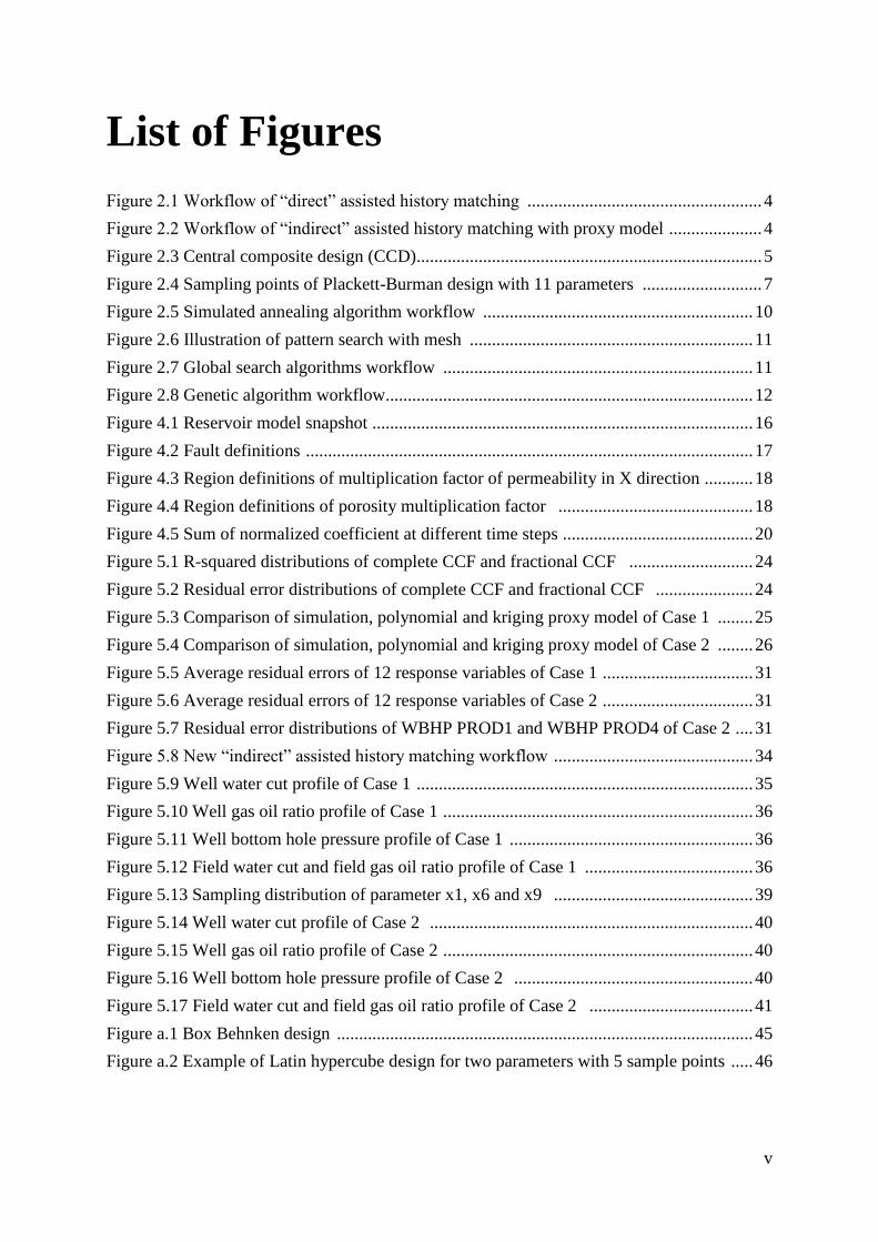
List of Figures

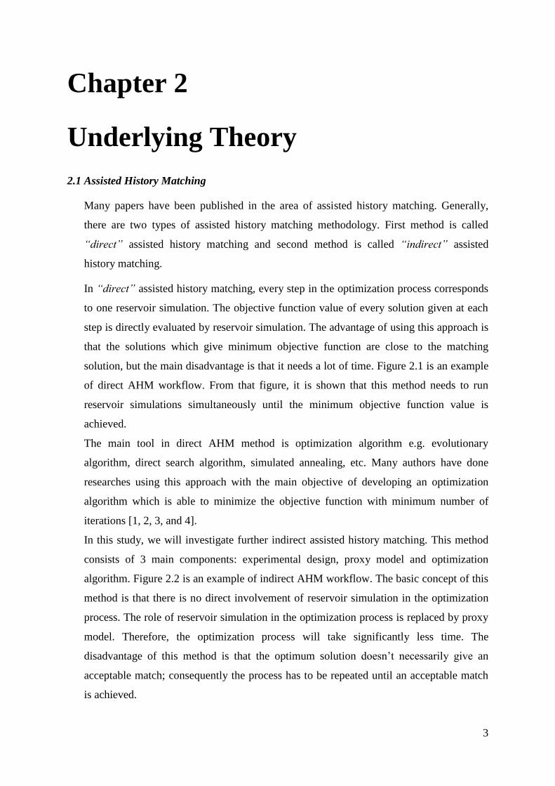
Figure 2.1 Workflow of “direct” assisted history matching ..................................................... 4

Figure 2.2 Workflow of “indirect” assisted history matching with proxy model ..................... 4

Figure 2.3 Central composite design (CCD).............................................................................. 5

Figure 2.4 Sampling points of Plackett-Burman design with 11 parameters ........................... 7

Figure 2.5 Simulated annealing algorithm workflow ............................................................. 10

Figure 2.6 Illustration of pattern search with mesh ................................................................ 11

Figure 2.7 Global search algorithms workflow ...................................................................... 11

Figure 2.8 Genetic algorithm workflow ................................................................................... 12

Figure 4.1 Reservoir model snapshot ...................................................................................... 16

Figure 4.2 Fault definitions ..................................................................................................... 17

Figure 4.3 Region definitions of multiplication factor of permeability in X direction ........... 18

Figure 4.4 Region definitions of porosity multiplication factor ............................................ 18

Figure 4.5 Sum of normalized coefficient at different time steps ........................................... 20

Figure 5.1 R-squared distributions of complete CCF and fractional CCF ............................ 24

Figure 5.2 Residual error distributions of complete CCF and fractional CCF ...................... 24

Figure 5.3 Comparison of simulation, polynomial and kriging proxy model of Case 1 ........ 25

Figure 5.4 Comparison of simulation, polynomial and kriging proxy model of Case 2 ........ 26

Figure 5.5 Average residual errors of 12 response variables of Case 1 .................................. 31

Figure 5.6 Average residual errors of 12 response variables of Case 2 .................................. 31

Figure 5.7 Residual error distributions of WBHP PROD1 and WBHP PROD4 of Case 2 .... 31

Figure 5.8 New “indirect” assisted history matching workflow ............................................. 34

Figure 5.9 Well water cut profile of Case 1 ............................................................................ 35

Figure 5.10 Well gas oil ratio profile of Case 1 ...................................................................... 36

Figure 5.11 Well bottom hole pressure profile of Case 1 ....................................................... 36

Figure 5.12 Field water cut and field gas oil ratio profile of Case 1 ...................................... 36

Figure 5.13 Sampling distribution of parameter x1, x6 and x9 ............................................. 39

Figure 5.14 Well water cut profile of Case 2 ......................................................................... 40

Figure 5.15 Well gas oil ratio profile of Case 2 ...................................................................... 40

Figure 5.16 Well bottom hole pressure profile of Case 2 ...................................................... 40

Figure 5.17 Field water cut and field gas oil ratio profile of Case 2 ..................................... 41

Figure a.1 Box Behnken design .............................................................................................. 45

Figure a.2 Example of Latin hypercube design for two parameters with 5 sample points ..... 46

vi

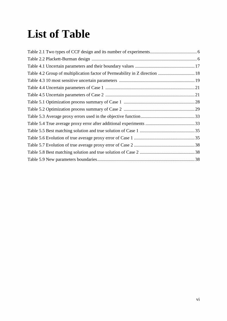
List of Table

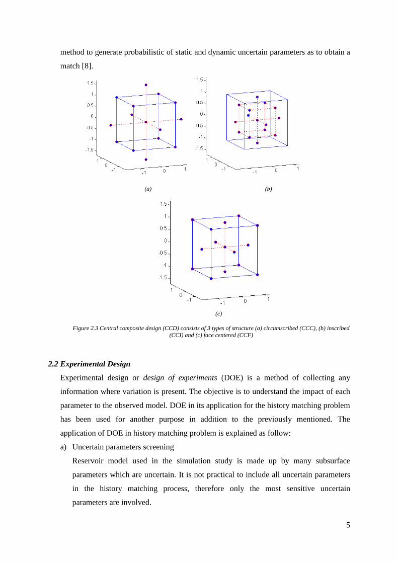
Table 2.1 Two types of CCF design and its number of experiments ......................................... 6

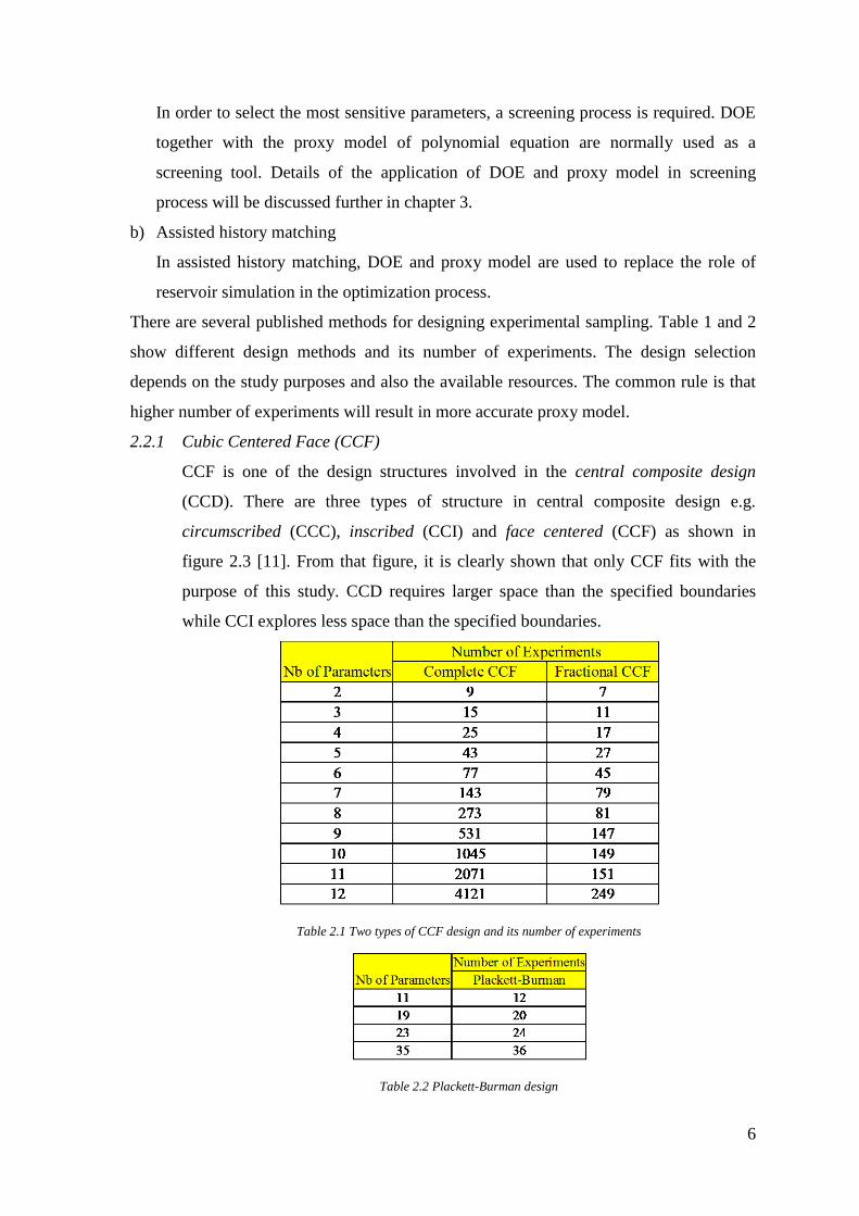
Table 2.2 Plackett-Burman design ............................................................................................ 6

Table 4.1 Uncertain parameters and their boundary values .................................................... 17

Table 4.2 Group of multiplication factor of Permeability in Z direction ................................ 18

Table 4.3 10 most sensitive uncertain parameters .................................................................. 19

Table 4.4 Uncertain parameters of Case 1 .............................................................................. 21

Table 4.5 Uncertain parameters of Case 2 .............................................................................. 21

Table 5.1 Optimization process summary of Case 1 .............................................................. 28

Table 5.2 Optimization process summary of Case 2 .............................................................. 29

Table 5.3 Average proxy errors used in the objective function ............................................... 33

Table 5.4 True average proxy error after additional experiments ........................................... 33

Table 5.5 Best matching solution and true solution of Case 1 ................................................ 35

Table 5.6 Evolution of true average proxy error of Case 1 ..................................................... 35

Table 5.7 Evolution of true average proxy error of Case 2 ..................................................... 38

Table 5.8 Best matching solution and true solution of Case 2 ................................................ 38

Table 5.9 New parameters boundaries ..................................................................................... 38

1

Chapter 1

Introduction

1.1 Study Background

Reservoir simulation plays an important role in the petroleum industry. Its common

applications are calculation of petroleum reserves and prediction of petroleum production.

Since reserves and production profiles are the two most important figures in the

petroleum business, it is important that reservoir simulation gives output with an

acceptable degree of accuracy. To achieve an accurate prediction of both reserves and

production profiles, the reservoir model used in the simulation must be reliable.

The only way of obtaining a reliable reservoir model is by doing history matching.

History matching is a tuning process of reservoir model by adjusting values of uncertain

reservoir parameters in order to achieve a better match between simulated and

observation data. In conventional history matching, the engineer adjusts the value of

uncertain reservoir parameters manually by trial and error until a sufficient match is

achieved. In most cases, history matching is a delicate, exhaustive and time consuming

process and furthermore in some cases it is difficult to achieve an acceptable match with

the conventional approach.

Assisted History Matching (AHM) consists of optimization techniques which

automatically adjust uncertain reservoir parameters until stopping criteria are achieved.

The aim is to make history matching less time consuming and more reliable. The AHM

procedures studied in this work involve the use of experimental design, proxy model and

optimization algorithm as the tools for finding the matching solutions. It is important that

the engineer has a comprehensive understanding of the AHM methodology before they

use it to solve history matching problem. Therefore, in this study a comprehensive

investigation of the methodology is emphasized.

1.2 Study Objectives

This study is set to achieve the following objectives:

a) Basic understanding of the concepts involved in the methodology

2

b) Identify limitations of the existing workflow so that some improvements can be

carried out

c) Investigate different types of experimental design methods, different proxy models

and different global optimization algorithms

The result of this study will be a comprehensive explanation of the methodology, some

improvements of the existing workflow enabling acceleration of the matching process, the

selection of the best proxy model and the global optimization algorithm.

1.3 Thesis outlines

This thesis report consists of six chapters. Chapter 1 includes discussion of the general

study background, the objectives to be achieved and the outline of the thesis report.

Underlying theory is covered in chapter 2. In this chapter, the discussion begins with the

review of published studies in the AHM area. Then it is continued with the explanation of

three main components in AHM methodology e.g. experimental design, proxy model and

global optimization algorithm.

Chapter 3 comprises detail explanation of AHM methodology used in this study. In

addition, an assisted history matching toolbox which was developed to conduct this study

is also explained in this chapter.

Chapter 4 discuses about an artificial 3D reservoir model which was developed as history

matching cases. These cases will be matched by using the proposed AHM methodology.

This chapter also includes detail information about uncertain parameters used in history

matching cases.

Discussions of the results are further elaborated in chapter 5. This chapter covers a deep

investigation of the methodology, improvements of the existing workflow and

comparison analysis of different experimental designs, proxy models and global

optimization algorithms. In addition, the matching process of the two study cases is also

shown in this chapter. Summary, conclusions and possible future works will be elaborated

in the chapter 6.

3

Chapter 2

Underlying Theory

2.1 Assisted History Matching

Many papers have been published in the area of assisted history matching. Generally,

there are two types of assisted history matching methodology. First method is called

“direct” assisted history matching and second method is called “indirect” assisted

history matching.

In “direct” assisted history matching, every step in the optimization process corresponds

to one reservoir simulation. The objective function value of every solution given at each

step is directly evaluated by reservoir simulation. The advantage of using this approach is

that the solutions which give minimum objective function are close to the matching

solution, but the main disadvantage is that it needs a lot of time. Figure 2.1 is an example

of direct AHM workflow. From that figure, it is shown that this method needs to run

reservoir simulations simultaneously until the minimum objective function value is

achieved.

The main tool in direct AHM method is optimization algorithm e.g. evolutionary

algorithm, direct search algorithm, simulated annealing, etc. Many authors have done

researches using this approach with the main objective of developing an optimization

algorithm which is able to minimize the objective function with minimum number of

iterations [1, 2, 3, and 4].

In this study, we will investigate further indirect assisted history matching. This method

consists of 3 main components: experimental design, proxy model and optimization

algorithm. Figure 2.2 is an example of indirect AHM workflow. The basic concept of this

method is that there is no direct involvement of reservoir simulation in the optimization

process. The role of reservoir simulation in the optimization process is replaced by proxy

model. Therefore, the optimization process will take significantly less time. The

disadvantage of this method is that the optimum solution doesn’t necessarily give an

acceptable match; consequently the process has to be repeated until an acceptable match

is achieved.

4

Figure 2.1 Workflow of “direct” assisted history matching

Figure 2.2 Workflow of “indirect” assisted history matching with proxy model

Experimental design is used to generate initial experiments. The initial experiments are

the basis of creating a proxy model. The proxy model will replace reservoir simulation in

the optimization process. The optimization algorithm searches optimum solutions which

give minimum objective function. However, these optimum solutions do not necessarily

give an acceptable match and the optimization has to be repeated with an improved proxy

model. The proxy model is improved by adding the optimum solutions to the initial

experiments. This recursive procedure is stopped when an acceptable match is achieved.

Related works about indirect AHM have been published in SPE paper [5, 6, 7, 8, and 9]

where each researcher focused on different subjects of this method. Baoyan Li and F.

Friedmann studied proxy model [9] and L. den Boer et al used experimental design

1. Perform reservoir

simulation of base

case run

(Iter 0)

2. Optimization

3. New solution is

produced

( Iter = iter +1 )

5. Minimum

objective function

or maximum

number of iteration

is achieved

6. Finish

Yes

No

4. Perform reservoir

simulation

1. Design initial

experiments (CCF,

Box-Behnken,

Latin Hypercube,

etc)

2. Perform reservoir

simulations

3. Build proxy model

with fitting

regression model

(kriging,

polynomial, etc)

4. Use optimization

algorithm to

minimize the

objective function

5. Set of solutions

are generated from

the optimization

process

6. Perform reservoir

simulations

7. Check if the

solutions have

given an

acceptable match

9. Update the proxy

modelFinish

Yes

No

5

method to generate probabilistic of static and dynamic uncertain parameters as to obtain a

match [8].

(a) (b)

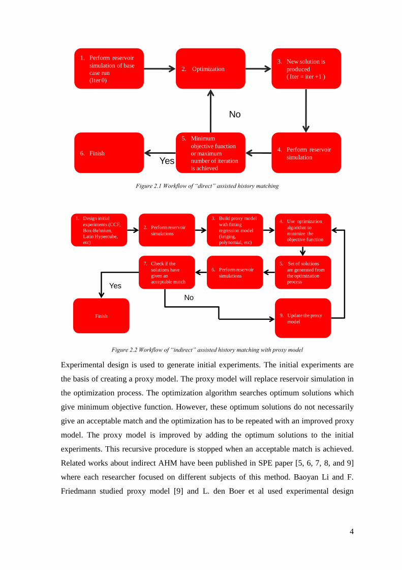
(c)

Figure 2.3 Central composite design (CCD) consists of 3 types of structure (a) circumscribed (CCC), (b) inscribed

(CCI) and (c) face centered (CCF)

2.2 Experimental Design

Experimental design or design of experiments (DOE) is a method of collecting any

information where variation is present. The objective is to understand the impact of each

parameter to the observed model. DOE in its application for the history matching problem

has been used for another purpose in addition to the previously mentioned. The

application of DOE in history matching problem is explained as follow:

a) Uncertain parameters screening

Reservoir model used in the simulation study is made up by many subsurface

parameters which are uncertain. It is not practical to include all uncertain parameters

in the history matching process, therefore only the most sensitive uncertain

parameters are involved.

6

In order to select the most sensitive parameters, a screening process is required. DOE

together with the proxy model of polynomial equation are normally used as a

screening tool. Details of the application of DOE and proxy model in screening

process will be discussed further in chapter 3.

b) Assisted history matching

In assisted history matching, DOE and proxy model are used to replace the role of

reservoir simulation in the optimization process.

There are several published methods for designing experimental sampling. Table 1 and 2

show different design methods and its number of experiments. The design selection

depends on the study purposes and also the available resources. The common rule is that

higher number of experiments will result in more accurate proxy model.

2.2.1 Cubic Centered Face (CCF)

CCF is one of the design structures involved in the central composite design

(CCD). There are three types of structure in central composite design e.g.

circumscribed (CCC), inscribed (CCI) and face centered (CCF) as shown in

figure 2.3 [11]. From that figure, it is clearly shown that only CCF fits with the

purpose of this study. CCD requires larger space than the specified boundaries

while CCI explores less space than the specified boundaries.

Table 2.1 Two types of CCF design and its number of experiments

Table 2.2 Plackett-Burman design

7

Generally, CCF design consists of a 2k full factorial (or 2

k-p fractional factorial

with 1/2p fraction) with nf runs, 2k axial or star runs and 1 center run with k is the

number of parameters [10]. An example with k=5, for complete CCF design there

are 25 runs plus 10 star runs and 1 center run, therefore by total there are 43

experiments. For the case of fractional CCF with ½ fractions the number of

experiments is calculated as follow, 25-1

= 16 runs plus 10 star runs and 1 center

run, therefore by total there are 27 experiments.

2.2.2 Plackett-Burman

Plackett-Burman is another design method which is used in this study. This

design is two level factorials design. For studying k= N-1 variables in N runs,

where N is the multiple of 4 e.g. N = 12, 16, 20, 24. Figure 2.4 shows the example

of the design sampling with 11 parameters. Plackett-Burman is a dedicated design

for fitting first order model. It is aimed to find the influence of the main effect of

each parameter. It requires less number of experiments for large number of

parameters involved. For the other experimental design methods are provided in

the appendix.

Figure 2.4 sampling points of Plackett-Burman design with 11 parameters

2.3 Proxy Model

The results from the experiments are then modeled with an empirical equation. This

equation can be used for at least two purposes. First, the equation generated can be used

to determine the sensitivity of each parameter and it is normally applied in parameter

8

screening process. Second, the empirical equation can also be used to replace real

experiment/simulation in order to predict the response of non sampling points.

In this study, there are two types of empirical equation that will be investigated e.g.

polynomial equation and kriging equation. By the end of this study, one of the equations

will be recommended as the proxy model in the AHM workflow.

2.3.1 Polynomial Equation

Equation 2.1 and 2.2 are two types of polynomial equation. Equation 2.1 is first

order polynomial equation while equation 2.2 is second order polynomial

equation.

n

i

iio xY1

……………………………………………... (2.1)

l

n

k

n

l

kkl

n

j

jj

n

i

iio xxxxY

1

1

111

………………… (2.2)

The values of coefficient βi, βj, βkl are determined through least square method

which minimizes the sum of the deviations between the predicted value and the

real value [12]. Index “n” in equation 2.1 and 2.2 is the number of parameters.

2.3.2 Ordinary Kriging Equation

Kriging is a popular method to solve spatial prediction problem. It is commonly

used for predicting the value of non sampling point. Equation 2.4 shows the

kriging system where the property’s value of non sampling points (s0) is a

weighted average of the property’s value of sampling points (si) [13]. Distance is

used as variogram model. Details equation can be seen in appendix.

…………………………………………… (2.3)

For the application in AHM, some adjustments have to be made especially at the

parameters scale. The scale of the uncertain parameters has to be normalized with

the same maximum and minimum values as it is the in real spatial problem.

2.4 Global Optimization Algorithm

Optimization algorithm has an important role in solving history matching problem. It

helps the engineer to find the solutions which could give an acceptable match to the

historical data. However, sometimes, several algorithms are trapped in the local minima

before they could find the matching solutions. Therefore, in this study, different

)()(1

0

^

n

i

ii sZwsZ

9

algorithms are investigated to see which algorithm is able to find the matching solutions

without being trapped in the local minima.

Four global optimization algorithms are selected in this study e.g. simulated annealing,

genetic algorithm, direct search, and global search algorithm. These algorithms can be

found in the Global Optimization Toolbox MatLab™.

2.4.1 Simulated Annealing Algorithm

Simulated annealing is an algorithm for solving constrained or unconstrained

optimization problems. The basic concept of simulated annealing is a model of

heating material and then slowly lowering the temperature to decrease defects,

thus minimizing the system energy [14].

The main parameter in this algorithm is temperature. Temperature significantly

influences the algorithm in a way such that not to get trapped in local minima. At

the beginning of the program an initial temperature is set, then cooling rate is

applied in order to reduce the temperature so that it can achieve a convergence.

…………………………………….. (2.4)

…………………… (2.5)

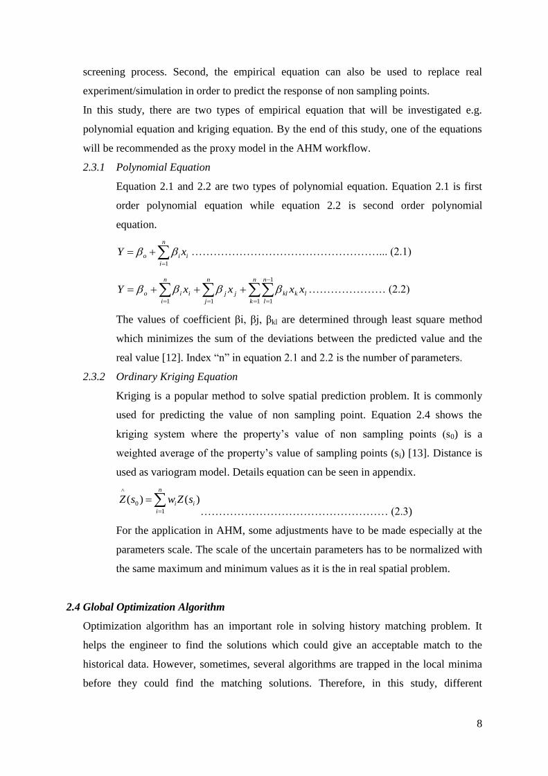
Figure 2.5 shows the workflow of simulated annealing algorithm. New solution

which is random neighboring points of current solutions is generated in order to

compare their objective function value. If the objective function of new solution is

smaller than current solution then this new solution becomes best solution so far.

Nevertheless, in order to avoid to get trapped in local minima, current solution

could still become best solution if the evaluation criterion of the probability

function is met (equation 2.9 and 2.10). For the next iteration temperature is

reduced by specified cooling rate.

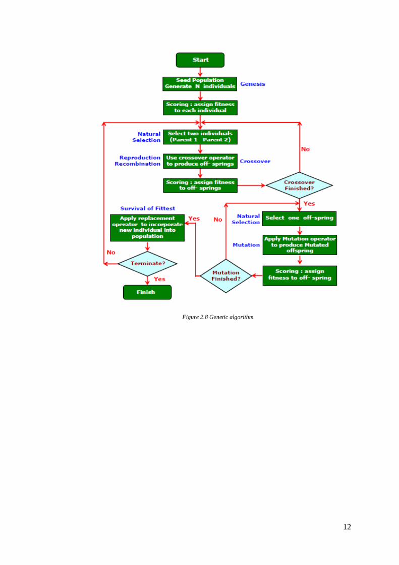
2.4.2 Genetic Algorithm

Genetic algorithm is a powerful, domain independent, search technique that was

inspired by Darwinian Theory [15]. Genetic algorithm is population based

algorithm which means that at each iteration more than one solution are created.

The basic concept of this algorithm is natural selection that strong individuals are

more survive and will also inherit their strong characteristics to their offspring.

There are two main genetic operators in this algorithm e.g. crossover and

mutation. Crossover is a genetic operator which provides mechanism for the

offspring to inherit characteristics of both parents. Mutation is a probabilistic

TFObjevalueRandom /

)()( CurSolFObjNewSolFObjFObj

10

based operator, which happen to some individuals in population. By having

mutation, new characteristics are introduced into the population which they don’t

inherit from their parents. Genetic algorithm scheme is shown in figure 2.8 [16].

Figure 2.5 Simulated annealing algorithm workflow

2.4.3 Direct Search Algorithm

Another global optimization algorithm is direct search algorithm. Mechanism in

direct search algorithm is that it searches a set of points around the current points

which gives lower value of objective function than current point. At each step, the

algorithm searches a set of points, called a mesh, around the current point. The

mesh is formed by adding the current point to a scalar multiple of a set of vectors

called a pattern. If the pattern search algorithm finds a point in the mesh that

improves the objective function at the current point, the new point becomes the

current point at the next step of the algorithm [16].

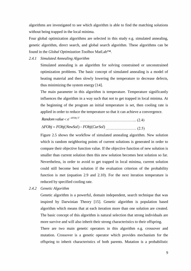
Figure 2.6 shows a current solution (red dot) and the rectangle which consists of

four possible solutions (black dot) forms a mesh network. In each step, possible

solutions in the current mesh are evaluated. The best solution will become current

solution for the next iteration. Also at each iteration mesh size is always updated,

basically if the current mesh could give a better solution than the current solution

then the mesh size will be bigger in the next iteration, but if a better solution could

not be found in the current mesh then the mesh size is reduced in the next

iteration.

Current solution

(CurSol) & current

temperature

Generate new solution

(NewSol)

Fobj(NewSol) <

Fobj(CurSol)

BestSol=NewSol

Cursol=NewSolUpdate temperature

Evaluate Probability

Function f(temperature)

BestSol=CurSol

Cursol=CurSol

Stopping criteria

achieved ?

Finish

Yes

NoYes

No

Yes

No

11

Figure 2.6 Illustration of pattern search with mesh

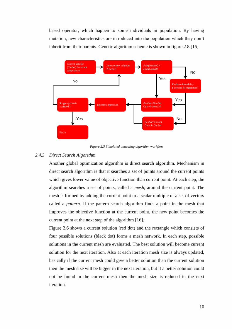
2.4.4 Global Search Algorithm

Global search algorithm has more complex algorithm than the three previous

algorithms. Basic concept of global search is actually local solver, different trial

points are generated using scatter search algorithm [17], these trial points later

becomes candidate of starting point for local solver if they are likely to improve

the best local minimum so far [14]. Figure 2.7 [14] is a diagram on how global

search algorithm works. Fmincon is local solver which is used in global search

collaborated with scatter search algorithm.

Figure 2.7 Global search algorithms workflow

12

Figure 2.8 Genetic algorithm

13

Chapter 3

Methodology Description

3.1 Methodology Workflow

Figure 2.2 shows a general workflow of assisted history matching that is investigated in

this study. There are at least 3 major components in the workflow. First is generation of

experimental design, second is generation of proxy model and the last component is

optimization process.

3.1.1 Initial Experiments

Initial experiments are required to build a proxy model. In AHM, common

methods used are CCF, Box Behnken and Latin Hypercube design. Initial

experiments play an important role in determining the quality of proxy model.

Basically, more initial experiments would result in a better proxy model. In this

study, two types of CCF design; fractional CCF and complete CCF are

investigated.

3.1.2 Proxy Model

Proxy model replaces the role of reservoir simulation in the optimization process.

Therefore, an accurate proxy model is required to have a good result from the

optimization. Several methods that can be used to generate a proxy model are

polynomial, kriging, EnKf and etc. In this study, only kriging and polynomial

proxy model are further researched.

Proxy model is basically built from set of empirical equations, either is kriging,

polynomial or other types of equation. The number of empirical equations required

to build proxy model is depends on the number of response variables and time

steps used. As an illustration, in this study there are 12 response variables used in

history matching process with 72 number of time steps, so there are 864 empirical

equations required.

3.1.3 Objective Function

In order to find a matching solution, we need to define an objective function.

Equation 3.1 shows the objective function used in this study. The value of

objective function shows an average percentage of error of all matching variables

14

and time steps. The consequence of using this objective function is not to involve

zero observation data.

%100/1

1

,

1

,, xYObsYObsYcalcWp

FObjp

t

ti

k

i

titii

…………………. (3.1)

datan observatio

modelproxy from response observe of value

factor weighting

variablesresponse ofnumber

steps timeofnumber

function objective

obs

calc

Y

Y

W

k

p

FObj

3.1.4 Global Optimization Algorithm

There are many available optimization algorithm but not all of them are powerful

enough to find the most optimum solution. Some algorithms are often getting

trapped in local minima before it could find the optimum solution. In this study,

four algorithms that are classified as global optimization algorithm in MatLab

Toolbox are researched further. Those algorithms are simulated annealing, direct

search, global search and genetic algorithm.

3.2 Assisted History Matching Toolbox

In order to conduct this study, a computer program is used to run the whole workflow.

Below are the main steps that need to be developed in the program:

a. Generation of experimental sampling

b. Generation of simulation input files

c. Importing simulation results and observation data

d. Generation of proxy model

e. Generation of objective function

f. Optimization

In order to do steps from point a to e, an Excel VBA based toolbox was developed. This

toolbox is able to generate sampling points from some design methods e.g. complete

CCF, fractional CCF, Latin hypercube, Box Behnken and Plackett-Burman. After

sampling points have been generated, the next step is to write simulation input file for all

those experiments. It would be time-consuming if the simulation input file is written

manually for every experiment. Therefore, this step is done automatically in the toolbox.

This toolbox also contains a program to import and format simulation results and

15

observation data before they are being processed. The main part of this toolbox is to

generate proxy model from previously entered simulation results and to create an

objective function. This toolbox is able to build both kriging and polynomial proxy

model. The optimization of the objective function is done in MatLab by using Global

Optimization Toolbox.

16

Chapter 4

Reservoir Model Description

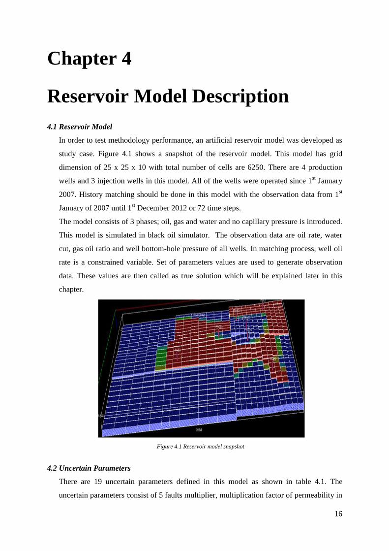
4.1 Reservoir Model

In order to test methodology performance, an artificial reservoir model was developed as

study case. Figure 4.1 shows a snapshot of the reservoir model. This model has grid

dimension of 25 x 25 x 10 with total number of cells are 6250. There are 4 production

wells and 3 injection wells in this model. All of the wells were operated since 1st January

2007. History matching should be done in this model with the observation data from 1st

January of 2007 until 1st December 2012 or 72 time steps.

The model consists of 3 phases; oil, gas and water and no capillary pressure is introduced.

This model is simulated in black oil simulator. The observation data are oil rate, water

cut, gas oil ratio and well bottom-hole pressure of all wells. In matching process, well oil

rate is a constrained variable. Set of parameters values are used to generate observation

data. These values are then called as true solution which will be explained later in this

chapter.

Figure 4.1 Reservoir model snapshot

4.2 Uncertain Parameters

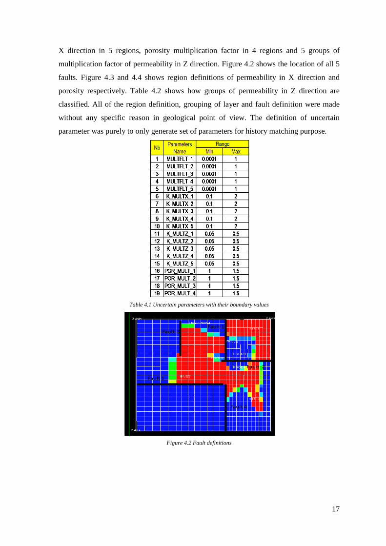
There are 19 uncertain parameters defined in this model as shown in table 4.1. The

uncertain parameters consist of 5 faults multiplier, multiplication factor of permeability in

17

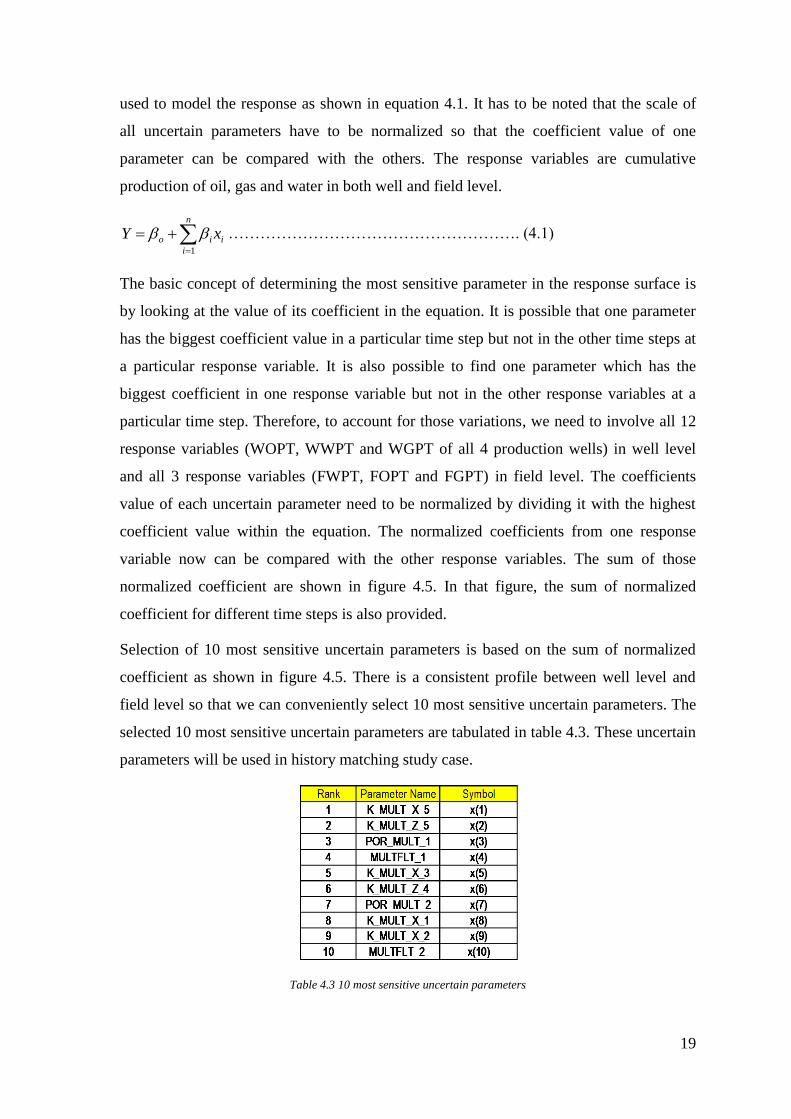
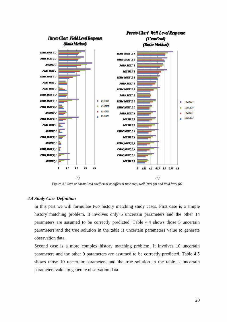
X direction in 5 regions, porosity multiplication factor in 4 regions and 5 groups of

multiplication factor of permeability in Z direction. Figure 4.2 shows the location of all 5

faults. Figure 4.3 and 4.4 shows region definitions of permeability in X direction and

porosity respectively. Table 4.2 shows how groups of permeability in Z direction are

classified. All of the region definition, grouping of layer and fault definition were made

without any specific reason in geological point of view. The definition of uncertain

parameter was purely to only generate set of parameters for history matching purpose.

Table 4.1 Uncertain parameters with their boundary values

Figure 4.2 Fault definitions

Fault 1

Fault 2

Fault 3

Fault 4

Fault 5

18

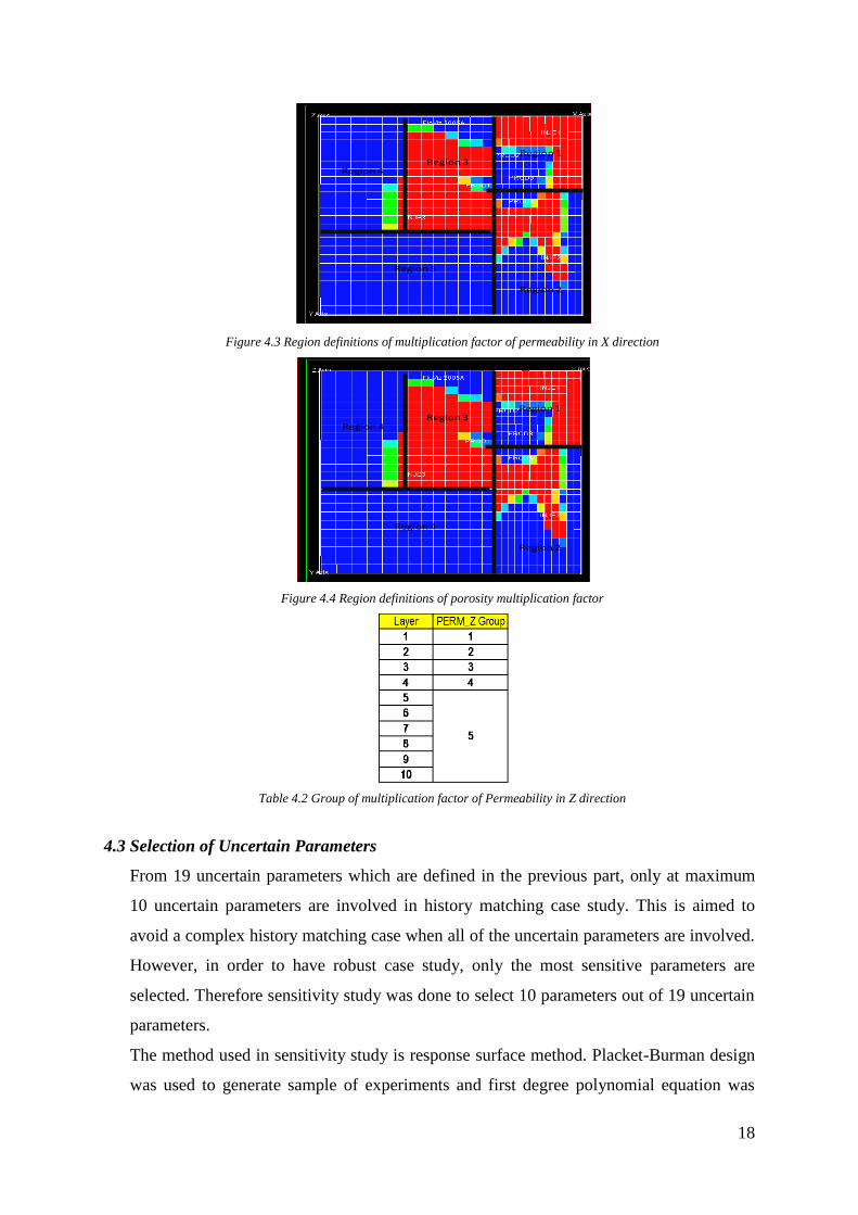
Figure 4.3 Region definitions of multiplication factor of permeability in X direction

Figure 4.4 Region definitions of porosity multiplication factor

Table 4.2 Group of multiplication factor of Permeability in Z direction

4.3 Selection of Uncertain Parameters

From 19 uncertain parameters which are defined in the previous part, only at maximum

10 uncertain parameters are involved in history matching case study. This is aimed to

avoid a complex history matching case when all of the uncertain parameters are involved.

However, in order to have robust case study, only the most sensitive parameters are

selected. Therefore sensitivity study was done to select 10 parameters out of 19 uncertain

parameters.

The method used in sensitivity study is response surface method. Placket-Burman design

was used to generate sample of experiments and first degree polynomial equation was

Region 1

Region 2

Region 3

Region 5

Region 4

Region 1

Region 2

Region 3

Region 4

Region 4

19

used to model the response as shown in equation 4.1. It has to be noted that the scale of

all uncertain parameters have to be normalized so that the coefficient value of one

parameter can be compared with the others. The response variables are cumulative

production of oil, gas and water in both well and field level.

n

i

iio xY1

………………………………………………. (4.1)

The basic concept of determining the most sensitive parameter in the response surface is

by looking at the value of its coefficient in the equation. It is possible that one parameter

has the biggest coefficient value in a particular time step but not in the other time steps at

a particular response variable. It is also possible to find one parameter which has the

biggest coefficient in one response variable but not in the other response variables at a

particular time step. Therefore, to account for those variations, we need to involve all 12

response variables (WOPT, WWPT and WGPT of all 4 production wells) in well level

and all 3 response variables (FWPT, FOPT and FGPT) in field level. The coefficients

value of each uncertain parameter need to be normalized by dividing it with the highest

coefficient value within the equation. The normalized coefficients from one response

variable now can be compared with the other response variables. The sum of those

normalized coefficient are shown in figure 4.5. In that figure, the sum of normalized

coefficient for different time steps is also provided.

Selection of 10 most sensitive uncertain parameters is based on the sum of normalized

coefficient as shown in figure 4.5. There is a consistent profile between well level and

field level so that we can conveniently select 10 most sensitive uncertain parameters. The

selected 10 most sensitive uncertain parameters are tabulated in table 4.3. These uncertain

parameters will be used in history matching study case.

Table 4.3 10 most sensitive uncertain parameters

20

(a) (b)

Figure 4.5 Sum of normalized coefficient at different time step, well level (a) and field level (b)

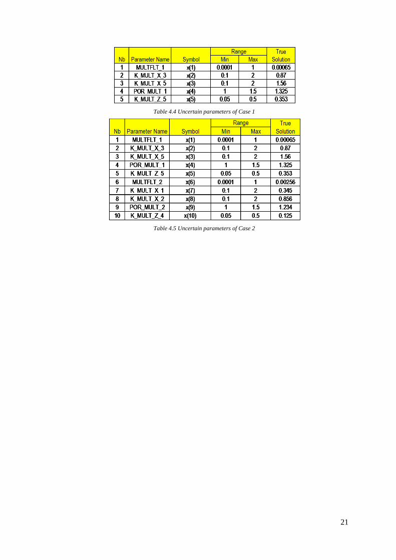
4.4 Study Case Definition

In this part we will formulate two history matching study cases. First case is a simple

history matching problem. It involves only 5 uncertain parameters and the other 14

parameters are assumed to be correctly predicted. Table 4.4 shows those 5 uncertain

parameters and the true solution in the table is uncertain parameters value to generate

observation data.

Second case is a more complex history matching problem. It involves 10 uncertain

parameters and the other 9 parameters are assumed to be correctly predicted. Table 4.5

shows those 10 uncertain parameters and the true solution in the table is uncertain

parameters value to generate observation data.

21

Table 4.4 Uncertain parameters of Case 1

Table 4.5 Uncertain parameters of Case 2

22

Chapter 5

Results Discussions

This chapter consists of three main discussion topics. The first discussion is methodology

validation which comprises comparison of several methods in experimental design, proxy

model and global optimization algorithm. Second discussion is about the workflow

improvements which are aimed to accelerate the matching process. The matching results of

the two study cases are explained in the last discussion topic.

5.1 Methodology Validation

The three main concepts which are introduced in the previous chapter e.g. experimental

design, proxy model and global optimization algorithm will be studied further in this

section.

5.1.2 Selection of Experimental Design Method

Initial experiments are the basis for creating a proxy model. A proxy model is

represented as a second degree polynomial equation. For the purpose of this study,

it is necessary to have a good proxy model. Therefore, two methods of

experimental design are studied in order to investigate the accuracy of proxy

model generated from each method.

R-squared and residual errors are used as the main criteria to assess the quality of

proxy model. The criteria can be explained as follow:

a. R-squared

The R squared value is a measure of how well observed outcomes are

reproduced by the model, as the proportion of total variation of outcomes

explained by the model. The closer the magnitude of r squared to unity then

the more the correlation between proxy model and real simulation results.

b. Residual error

In addition to r squared criteria, an accurate proxy model would also have

residual error close to zero. The equation of r squared and residual error are

presented in equation 5.1 and 5.2.

23

n

i

icalcisim

n

i

isimicalc

yy

yy

R

1

2

,,

1

2

,,2

)(

)(

1 ………………………………………… (5.1)

%100(%) xy

yyRS

sim

simcalc ………………………………………… (5.2)

datan observatio

modelproxy of response observe of value

sexperiment ofnumber n

error residual

obs

calc

Y

Y

RS

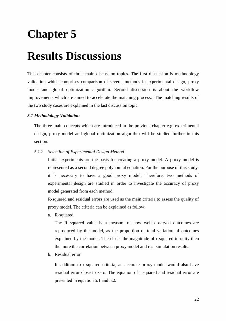
Complete CCF design is used in Case 1 which results in 43 initial experiments.

For Case 2, because it involves 10 uncertain parameters, fractional CCF design is

employed in order to have a practical number of initial experiments (149 initial

experiments). The proxy models were generated for 12 response variables and 72

time steps.

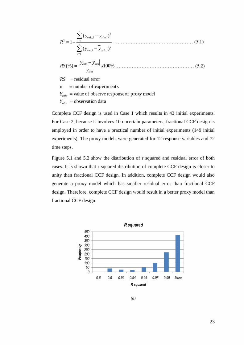
Figure 5.1 and 5.2 show the distribution of r squared and residual error of both

cases. It is shown that r squared distribution of complete CCF design is closer to

unity than fractional CCF design. In addition, complete CCF design would also

generate a proxy model which has smaller residual error than fractional CCF

design. Therefore, complete CCF design would result in a better proxy model than

fractional CCF design.

(a)

050

100150200250300350400450

0.6 0.9 0.92 0.94 0.96 0.98 0.99 More

Fre

qu

ency

R squared

R squared

24

(b)

Figure 5.1 R-squared distributions of complete CCF (a) and fractional CCF (b)

(a)

(b)

Figure 5.2 Residual error distributions of complete CCF (a) and fractional CCF (b)

0

100

200

300

400

500

600

0.6 0.9 0.92 0.94 0.96 0.98 0.99 More

Fre

qu

ency

R Squared

R squared

0

5000

10000

15000

20000

25000

Fre

qu

en

cy

Residual error (%)

Residual Error Distribution

0

100002000030000

40000

50000

60000

70000

8000090000

0.5 1

1.5 2

2.5 3

3.5 4

4.5 5

5.5 6

6.5 7

Mor

e

Fre

qu

ency

Residual Error (%)

Residual Error Distribution

25

5.1.3 Selection of Proxy Model

The quality of proxy model also depends on the fitting regression model. In this

study there are two proxy models that are investigated e.g. second degree

polynomial equation and ordinary kriging equation. The model which results in a

better proxy model will be used further for matching process.

In order to select the best proxy from the two models, a comparison to the

simulator is conducted. The true solution of the uncertain parameters in Case 1

and Case 2 are entered into second degree polynomial equation and kriging

equation. The profiles generated from the two equations are then compared with

the result from simulation.

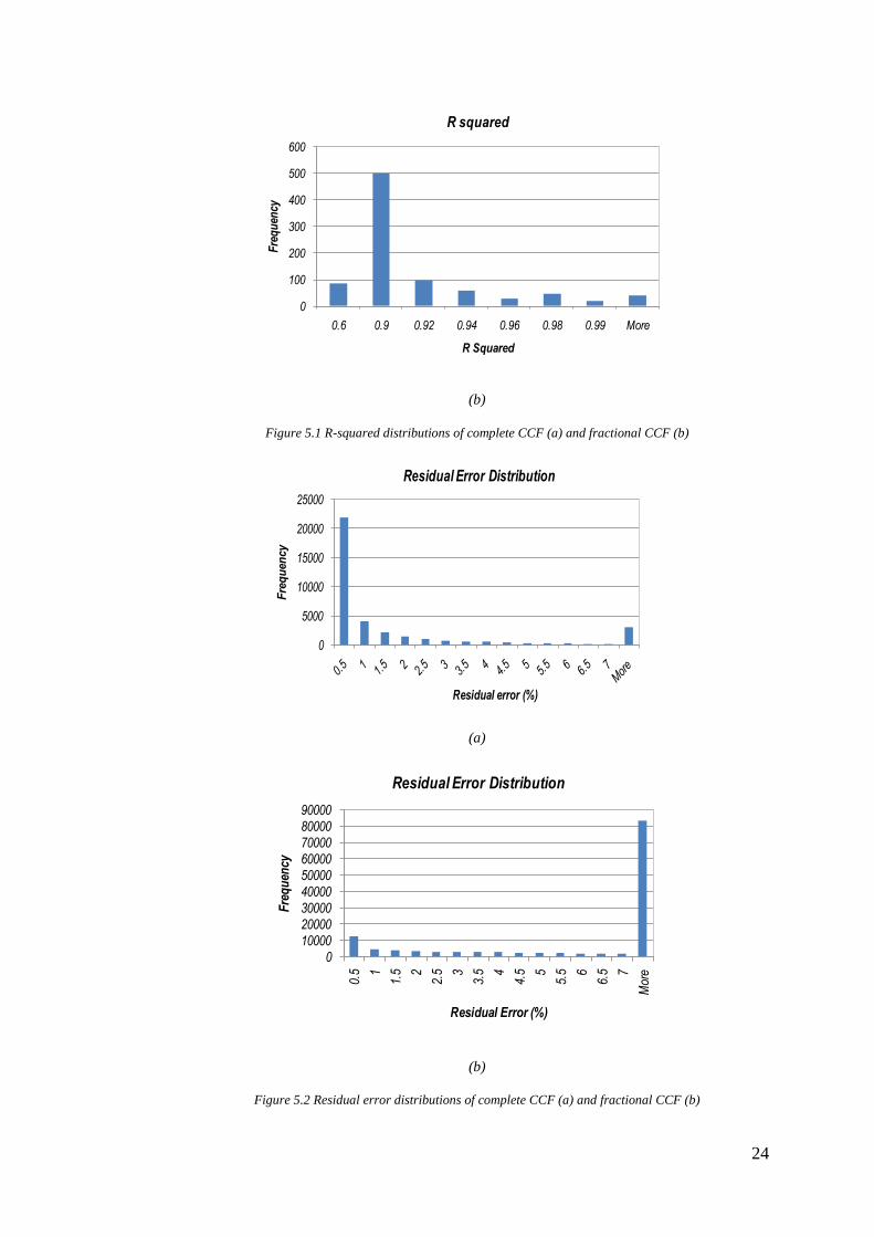
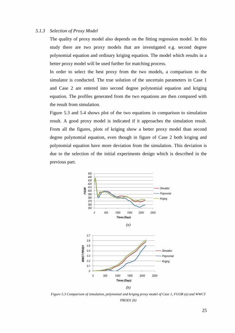
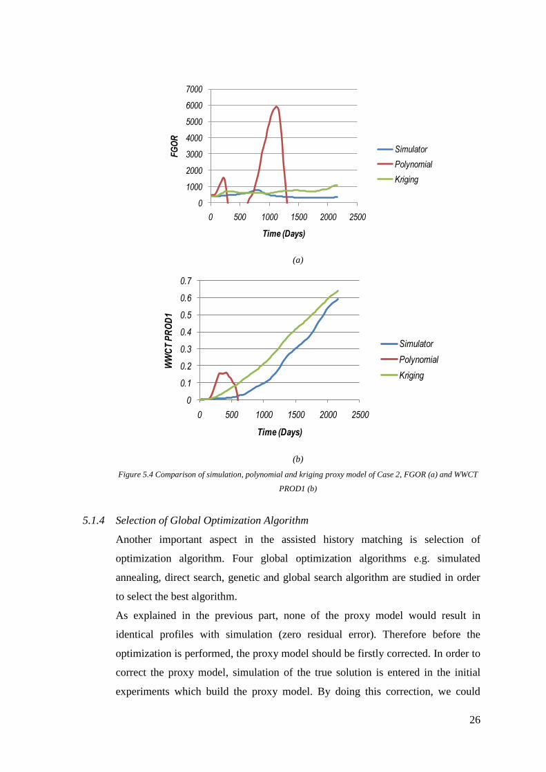
Figure 5.3 and 5.4 shows plot of the two equations in comparison to simulation

result. A good proxy model is indicated if it approaches the simulation result.

From all the figures, plots of kriging show a better proxy model than second

degree polynomial equation, even though in figure of Case 2 both kriging and

polynomial equation have more deviation from the simulation. This deviation is

due to the selection of the initial experiments design which is described in the

previous part.

(a)

(b)

Figure 5.3 Comparison of simulation, polynomial and kriging proxy model of Case 1, FGOR (a) and WWCT

PROD1 (b)

350

360

370

380

390

400

410

420

430

440

450

0 500 1000 1500 2000 2500

FG

OR

Times (Days)

Simulator

Polynomial

Kriging

0

0.1

0.2

0.3

0.4

0.5

0.6

0.7

0 500 1000 1500 2000 2500

WW

CT

PR

OD

1

Times (Days)

Simulator

Polynomial

Kriging

26

(a)

(b)

Figure 5.4 Comparison of simulation, polynomial and kriging proxy model of Case 2, FGOR (a) and WWCT

PROD1 (b)

5.1.4 Selection of Global Optimization Algorithm

Another important aspect in the assisted history matching is selection of

optimization algorithm. Four global optimization algorithms e.g. simulated

annealing, direct search, genetic and global search algorithm are studied in order

to select the best algorithm.

As explained in the previous part, none of the proxy model would result in

identical profiles with simulation (zero residual error). Therefore before the

optimization is performed, the proxy model should be firstly corrected. In order to

correct the proxy model, simulation of the true solution is entered in the initial

experiments which build the proxy model. By doing this correction, we could

0

1000

2000

3000

4000

5000

6000

7000

0 500 1000 1500 2000 2500

FG

OR

Time (Days)

Simulator

Polynomial

Kriging

0

0.1

0.2

0.3

0.4

0.5

0.6

0.7

0 500 1000 1500 2000 2500

WW

CT

PR

OD

1

Time (Days)

Simulator

Polynomial

Kriging

27

expect that the solution generated from the optimization has to be close to the true

solution.

Algorithm properties

In general, most properties of all algorithms are set as their default value in

MatLab Global Optimization Toolbox. Below are some changes that were made in

this study:

a. Maximum iteration (or generations for genetic algorithm) is 1000

b. Number of population for genetic algorithm is 50

c. Minimum changes of objective function value is 1e-6

Each of algorithms is given five attempts to find the true solution. In order to have

a robust optimization process, the initial solution is set to be random. The

summary of the optimization process are shown in Table 5.1 and 5.2. The main

comparison parameters are the value of objective function and the optimization

time. The best algorithm is the one which could generate smallest objective

function in a short processing time.

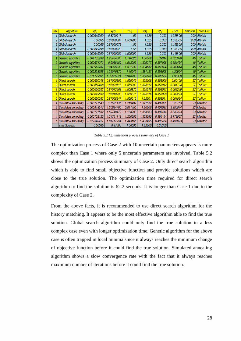
The optimization process of Case 1 can be seen in table 5.1. Global search

algorithm gives the least value of objective function around 0.0001 but it needs

200 second for one attempt of optimization. Direct search algorithm also generates

a small objective function less than 0.01 but with shorter processing time (27

seconds) than global search algorithm. The optimization process of direct search

algorithm stopped because the changes in objective function have reached the

minimum value. From five optimization attempts done by genetic algorithm, only

one generates a solution which is close to the true solution. Genetic algorithm

needs 46 seconds of optimization process before it stopped because of reaching

the minimum change of objective function. Simulated annealing algorithm

appears to be the worst since none of the generated solutions are close to the true

solution. It stopped the optimization process because maximum number of

iteration is reached. This is an indication that the convergence rate is slow.

28

Table 5.1 Optimization process summary of Case 1

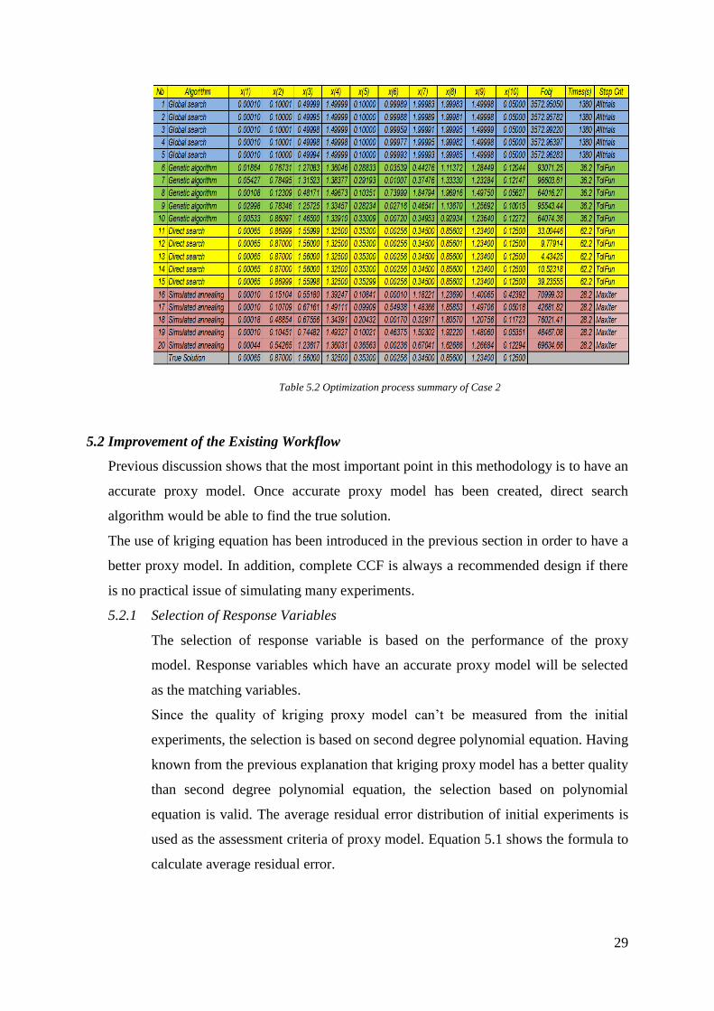
The optimization process of Case 2 with 10 uncertain parameters appears is more

complex than Case 1 where only 5 uncertain parameters are involved. Table 5.2

shows the optimization process summary of Case 2. Only direct search algorithm

which is able to find small objective function and provide solutions which are

close to the true solution. The optimization time required for direct search

algorithm to find the solution is 62.2 seconds. It is longer than Case 1 due to the

complexity of Case 2.

From the above facts, it is recommended to use direct search algorithm for the

history matching. It appears to be the most effective algorithm able to find the true

solution. Global search algorithm could only find the true solution in a less

complex case even with longer optimization time. Genetic algorithm for the above

case is often trapped in local minima since it always reaches the minimum change

of objective function before it could find the true solution. Simulated annealing

algorithm shows a slow convergence rate with the fact that it always reaches

maximum number of iterations before it could find the true solution.

29

Table 5.2 Optimization process summary of Case 2

5.2 Improvement of the Existing Workflow

Previous discussion shows that the most important point in this methodology is to have an

accurate proxy model. Once accurate proxy model has been created, direct search

algorithm would be able to find the true solution.

The use of kriging equation has been introduced in the previous section in order to have a

better proxy model. In addition, complete CCF is always a recommended design if there

is no practical issue of simulating many experiments.

5.2.1 Selection of Response Variables

The selection of response variable is based on the performance of the proxy

model. Response variables which have an accurate proxy model will be selected

as the matching variables.

Since the quality of kriging proxy model can’t be measured from the initial

experiments, the selection is based on second degree polynomial equation. Having

known from the previous explanation that kriging proxy model has a better quality

than second degree polynomial equation, the selection based on polynomial

equation is valid. The average residual error distribution of initial experiments is

used as the assessment criteria of proxy model. Equation 5.1 shows the formula to

calculate average residual error.

30

p

t

k

i

tititiij xYsimYsimYcalcWp 1 1

,,, %100/1

…………………… (5.3)

simulation of response observe of value

modelproxy of response observe of value

factor weighting

variablesresponse ofnumber

steps timeofnumber

j experiment oferror residual average

sim

calc

j

Y

Y

W

k

p

Below are examples of the selection process of Case 1 and Case 2:

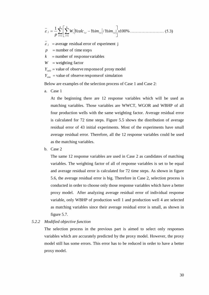
a. Case 1

At the beginning there are 12 response variables which will be used as

matching variables. Those variables are WWCT, WGOR and WBHP of all

four production wells with the same weighting factor. Average residual error

is calculated for 72 time steps. Figure 5.5 shows the distribution of average

residual error of 43 initial experiments. Most of the experiments have small

average residual error. Therefore, all the 12 response variables could be used

as the matching variables.

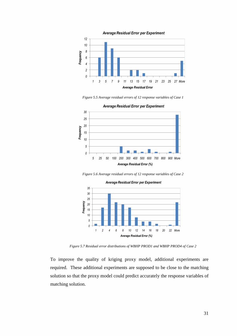
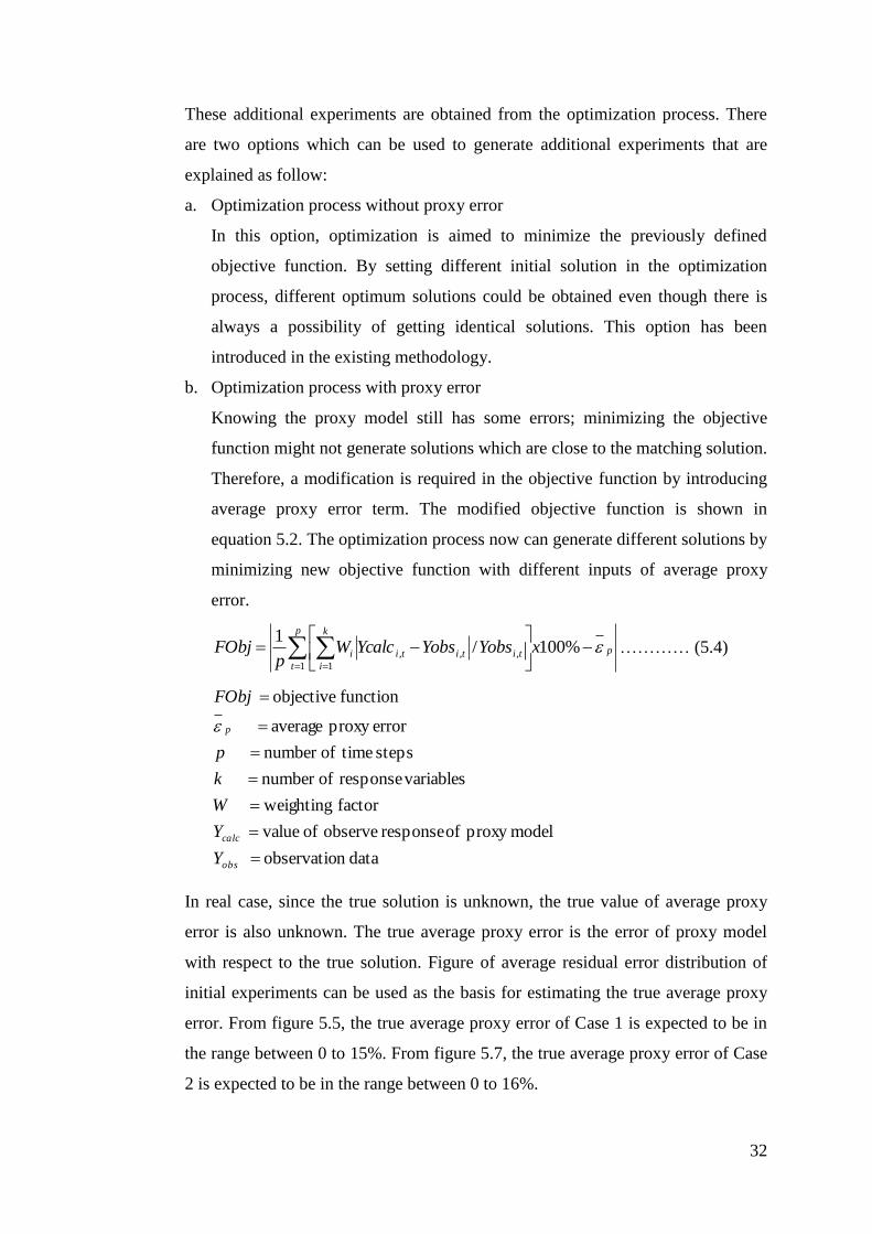
b. Case 2

The same 12 response variables are used in Case 2 as candidates of matching

variables. The weighting factor of all of response variables is set to be equal

and average residual error is calculated for 72 time steps. As shown in figure

5.6, the average residual error is big. Therefore in Case 2, selection process is

conducted in order to choose only those response variables which have a better

proxy model. After analyzing average residual error of individual response

variable, only WBHP of production well 1 and production well 4 are selected

as matching variables since their average residual error is small, as shown in

figure 5.7.

5.2.2 Modified objective function

The selection process in the previous part is aimed to select only responses

variables which are accurately predicted by the proxy model. However, the proxy

model still has some errors. This error has to be reduced in order to have a better

proxy model.

31

Figure 5.5 Average residual errors of 12 response variables of Case 1

Figure 5.6 Average residual errors of 12 response variables of Case 2

Figure 5.7 Residual error distributions of WBHP PROD1 and WBHP PROD4 of Case 2

To improve the quality of kriging proxy model, additional experiments are

required. These additional experiments are supposed to be close to the matching

solution so that the proxy model could predict accurately the response variables of

matching solution.

0

2

4

6

8

10

12

1 3 5 7 9 11 13 15 17 19 21 23 25 27 MoreF

req

uen

cy

Average Residual Error

Average Residual Error per Experiment

0

5

10

15

20

25

30

5 25 50 100 200 300 400 500 600 700 800 900 More

Fre

qu

ency

Average Residual Error (%)

Average Residual Error per Experiment

0

5

10

15

20

25

30

35

1 2 4 6 8 10 12 14 16 18 20 22 More

Fre

qu

ency

Average Residual Error (%)

Average Residual Error per Experiment

32

These additional experiments are obtained from the optimization process. There

are two options which can be used to generate additional experiments that are

explained as follow:

a. Optimization process without proxy error

In this option, optimization is aimed to minimize the previously defined

objective function. By setting different initial solution in the optimization

process, different optimum solutions could be obtained even though there is

always a possibility of getting identical solutions. This option has been

introduced in the existing methodology.

b. Optimization process with proxy error

Knowing the proxy model still has some errors; minimizing the objective

function might not generate solutions which are close to the matching solution.

Therefore, a modification is required in the objective function by introducing

average proxy error term. The modified objective function is shown in

equation 5.2. The optimization process now can generate different solutions by

minimizing new objective function with different inputs of average proxy

error.

p

p

t

k

i

tititii xYobsYobsYcalcWp

FObj

%100/1

1 1

,,, ………… (5.4)

datan observatio

modelproxy of response observe of value

factor weighting

variablesresponse ofnumber

steps timeofnumber

errorproxy average

function objective

obs

calc

p

Y

Y

W

k

p

FObj

In real case, since the true solution is unknown, the true value of average proxy

error is also unknown. The true average proxy error is the error of proxy model

with respect to the true solution. Figure of average residual error distribution of

initial experiments can be used as the basis for estimating the true average proxy

error. From figure 5.5, the true average proxy error of Case 1 is expected to be in

the range between 0 to 15%. From figure 5.7, the true average proxy error of Case

2 is expected to be in the range between 0 to 16%.

33

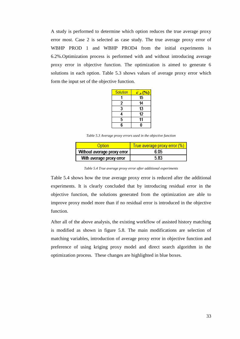
A study is performed to determine which option reduces the true average proxy

error most. Case 2 is selected as case study. The true average proxy error of

WBHP PROD 1 and WBHP PROD4 from the initial experiments is

6.2%.Optimization process is performed with and without introducing average

proxy error in objective function. The optimization is aimed to generate 6

solutions in each option. Table 5.3 shows values of average proxy error which

form the input set of the objective function.

Table 5.3 Average proxy errors used in the objective function

Table 5.4 True average proxy error after additional experiments

Table 5.4 shows how the true average proxy error is reduced after the additional

experiments. It is clearly concluded that by introducing residual error in the

objective function, the solutions generated from the optimization are able to

improve proxy model more than if no residual error is introduced in the objective

function.

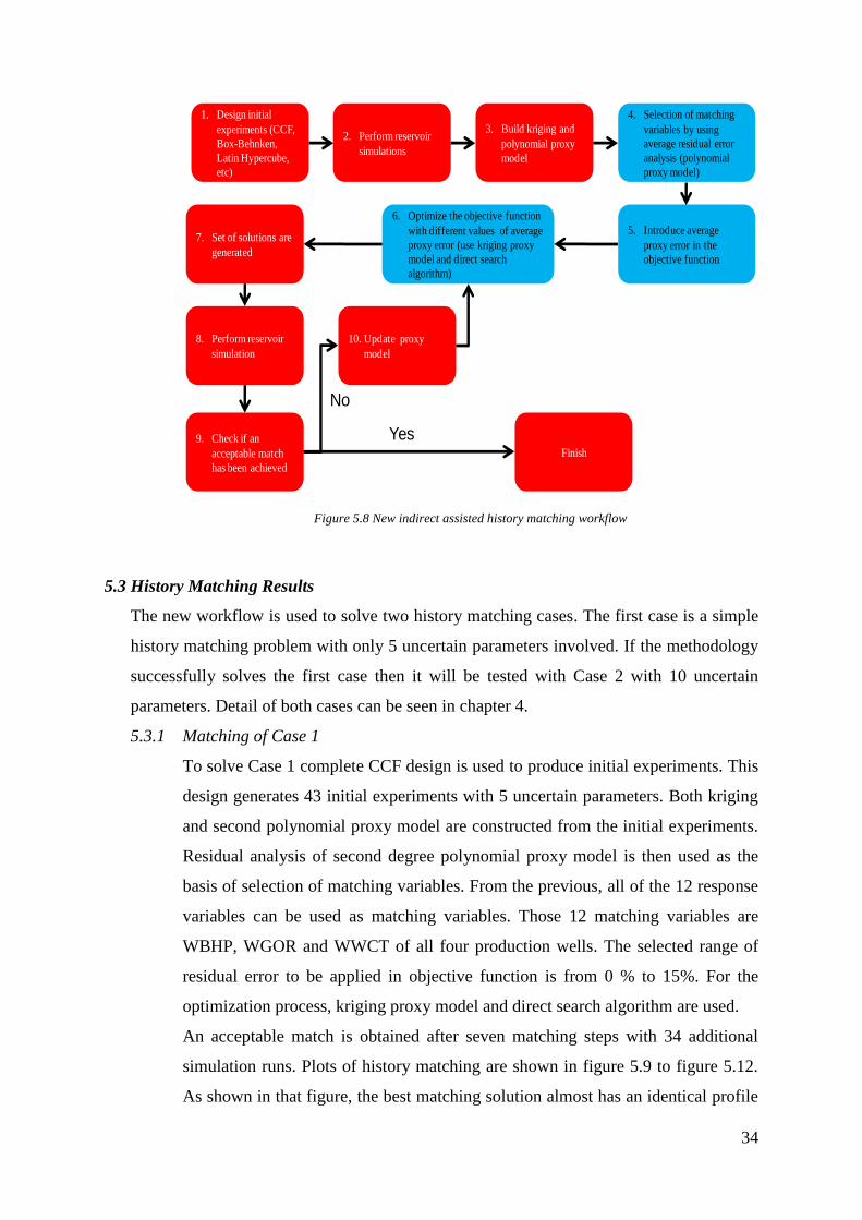
After all of the above analysis, the existing workflow of assisted history matching

is modified as shown in figure 5.8. The main modifications are selection of

matching variables, introduction of average proxy error in objective function and

preference of using kriging proxy model and direct search algorithm in the

optimization process. These changes are highlighted in blue boxes.

34

Figure 5.8 New indirect assisted history matching workflow

5.3 History Matching Results

The new workflow is used to solve two history matching cases. The first case is a simple

history matching problem with only 5 uncertain parameters involved. If the methodology

successfully solves the first case then it will be tested with Case 2 with 10 uncertain

parameters. Detail of both cases can be seen in chapter 4.

5.3.1 Matching of Case 1

To solve Case 1 complete CCF design is used to produce initial experiments. This

design generates 43 initial experiments with 5 uncertain parameters. Both kriging

and second polynomial proxy model are constructed from the initial experiments.

Residual analysis of second degree polynomial proxy model is then used as the

basis of selection of matching variables. From the previous, all of the 12 response

variables can be used as matching variables. Those 12 matching variables are

WBHP, WGOR and WWCT of all four production wells. The selected range of

residual error to be applied in objective function is from 0 % to 15%. For the

optimization process, kriging proxy model and direct search algorithm are used.

An acceptable match is obtained after seven matching steps with 34 additional

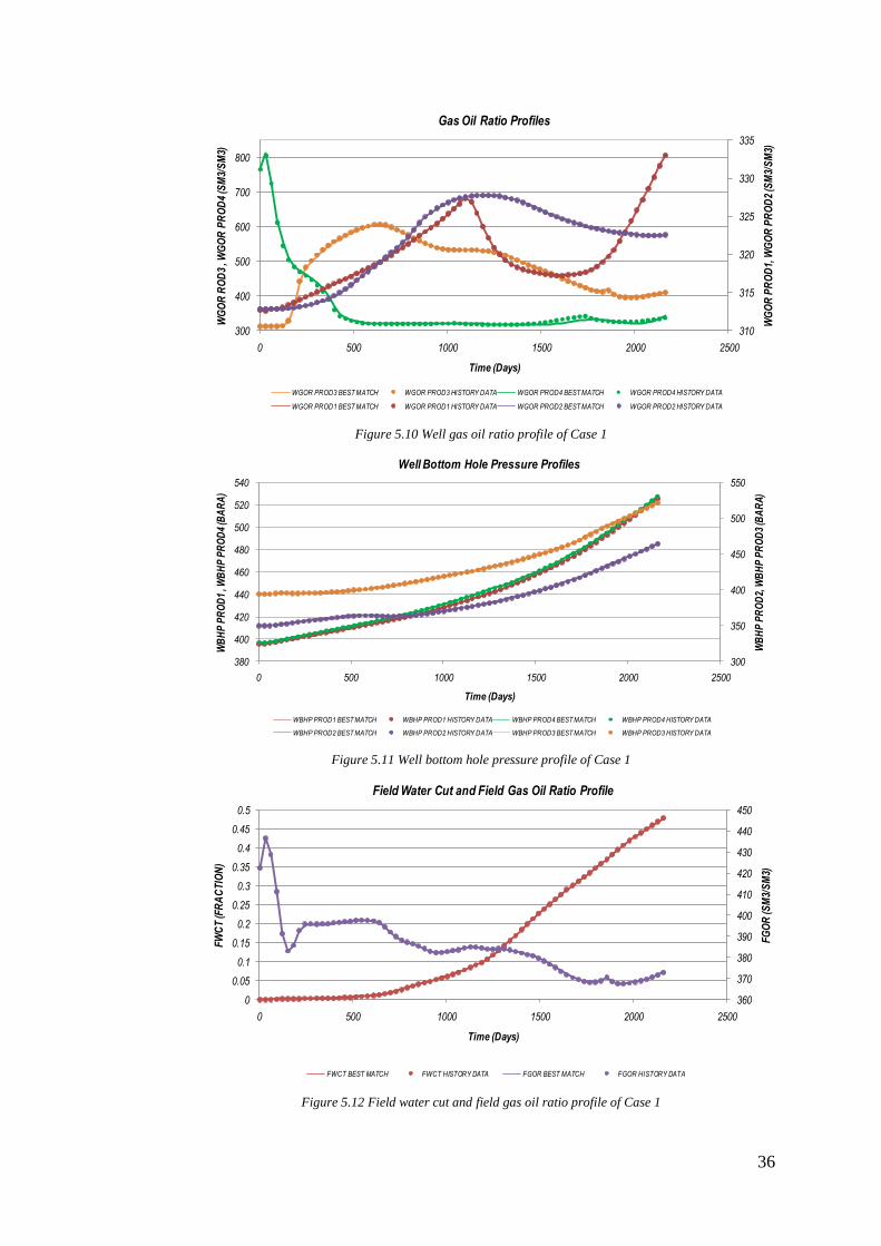
simulation runs. Plots of history matching are shown in figure 5.9 to figure 5.12.

As shown in that figure, the best matching solution almost has an identical profile

1. Design initial

experiments (CCF,

Box-Behnken,

Latin Hypercube,

etc)

2. Perform reservoir

simulations

3. Build kriging and

polynomial proxy

model

4. Selection of matching

variables by using

average residual error

analysis (polynomial

proxy model)

5. Introduce average

proxy error in the

objective function

6. Optimize the objective function

with different values of average

proxy error (use kriging proxy

model and direct search

algorithm)

7. Set of solutions are

generated

10. Update proxy

model

Finish

Yes

No

8. Perform reservoir

simulation

9. Check if an

acceptable match

has been achieved

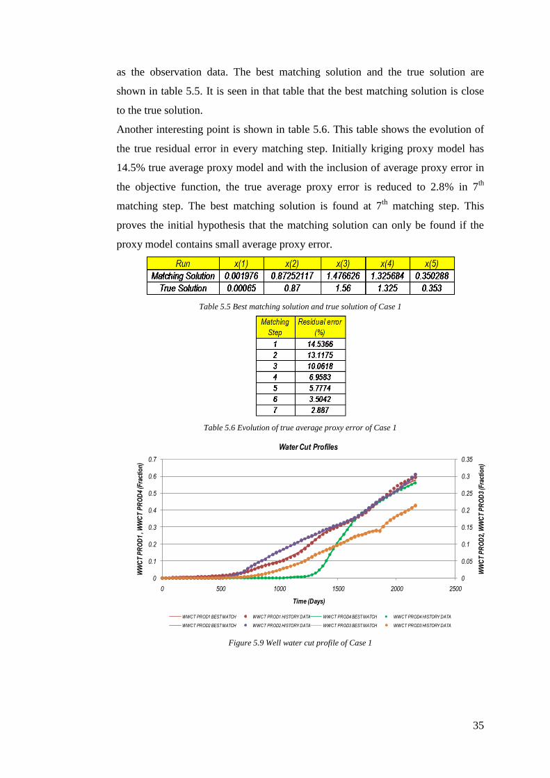
35

as the observation data. The best matching solution and the true solution are

shown in table 5.5. It is seen in that table that the best matching solution is close

to the true solution.

Another interesting point is shown in table 5.6. This table shows the evolution of

the true residual error in every matching step. Initially kriging proxy model has

14.5% true average proxy model and with the inclusion of average proxy error in

the objective function, the true average proxy error is reduced to 2.8% in 7th

matching step. The best matching solution is found at 7th

matching step. This

proves the initial hypothesis that the matching solution can only be found if the

proxy model contains small average proxy error.

Table 5.5 Best matching solution and true solution of Case 1

Table 5.6 Evolution of true average proxy error of Case 1

Figure 5.9 Well water cut profile of Case 1

0

0.05

0.1

0.15

0.2

0.25

0.3

0.35

0

0.1

0.2

0.3

0.4

0.5

0.6

0.7

0 500 1000 1500 2000 2500

WW

CT

PR

OD

2, W

WC

T P

RO

D3

(Fra

ctio

n)

WW

CT

PR

OD

1 , W

WC

T P

RO

D4

(Fra

ctio

n)

Time (Days)

Water Cut Profiles

WWCT PROD1 BEST MATCH WWCT PROD1 HISTORY DATA WWCT PROD4 BEST MATCH WWCT PROD4 HISTORY DATA

WWCT PROD2 BEST MATCH WWCT PROD2 HISTORY DATA WWCT PROD3 BEST MATCH WWCT PROD3 HISTORY DATA

36

Figure 5.10 Well gas oil ratio profile of Case 1

Figure 5.11 Well bottom hole pressure profile of Case 1

Figure 5.12 Field water cut and field gas oil ratio profile of Case 1

310

315

320

325

330

335

300

400

500

600

700

800

0 500 1000 1500 2000 2500

WG

OR

PR

OD

1, W

GO

R P

RO

D2

(SM

3/S

M3)

WG

OR

RO

D3

, WG

OR

PR

OD

4 (S

M3/

SM

3)

Time (Days)

Gas Oil Ratio Profiles

WGOR PROD3 BEST MATCH WGOR PROD3 HISTORY DATA WGOR PROD4 BEST MATCH WGOR PROD4 HISTORY DATA

WGOR PROD1 BEST MATCH WGOR PROD1 HISTORY DATA WGOR PROD2 BEST MATCH WGOR PROD2 HISTORY DATA

300

350

400

450

500

550

380

400

420

440

460

480

500

520

540

0 500 1000 1500 2000 2500

WB

HP

PR

OD

2, W

BH

P P

RO

D3

(BA

RA

)

WB

HP

PR

OD

1 , W

BH

P P

RO

D4

(BA

RA

)

Time (Days)

Well Bottom Hole Pressure Profiles

WBHP PROD1 BEST MATCH WBHP PROD1 HISTORY DATA WBHP PROD4 BEST MATCH WBHP PROD4 HISTORY DATA

WBHP PROD2 BEST MATCH WBHP PROD2 HISTORY DATA WBHP PROD3 BEST MATCH WBHP PROD3 HISTORY DATA

360

370

380

390

400

410

420

430

440

450

0

0.05

0.1

0.15

0.2

0.25

0.3

0.35

0.4

0.45

0.5

0 500 1000 1500 2000 2500

FG

OR

(SM

3/S

M3)

FW

CT

(FR

AC

TIO

N)

Time (Days)

Field Water Cut and Field Gas Oil Ratio Profile

FWCT BEST MATCH FWCT HISTORY DATA FGOR BEST MATCH FGOR HISTORY DATA

37

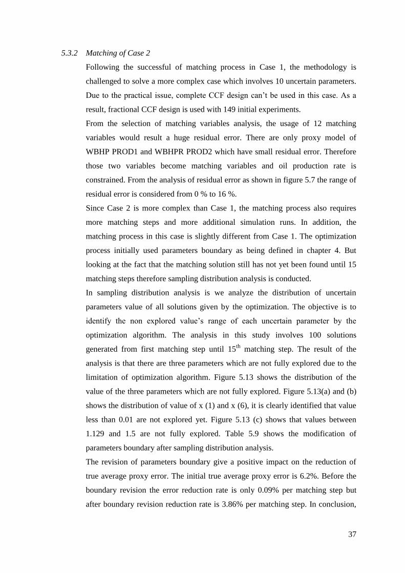
5.3.2 Matching of Case 2

Following the successful of matching process in Case 1, the methodology is

challenged to solve a more complex case which involves 10 uncertain parameters.

Due to the practical issue, complete CCF design can’t be used in this case. As a

result, fractional CCF design is used with 149 initial experiments.

From the selection of matching variables analysis, the usage of 12 matching

variables would result a huge residual error. There are only proxy model of

WBHP PROD1 and WBHPR PROD2 which have small residual error. Therefore

those two variables become matching variables and oil production rate is

constrained. From the analysis of residual error as shown in figure 5.7 the range of

residual error is considered from 0 % to 16 %.

Since Case 2 is more complex than Case 1, the matching process also requires

more matching steps and more additional simulation runs. In addition, the

matching process in this case is slightly different from Case 1. The optimization

process initially used parameters boundary as being defined in chapter 4. But

looking at the fact that the matching solution still has not yet been found until 15

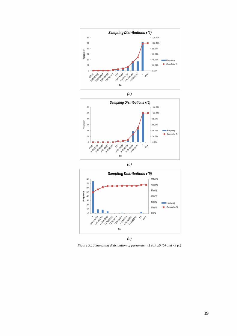
matching steps therefore sampling distribution analysis is conducted.

In sampling distribution analysis is we analyze the distribution of uncertain

parameters value of all solutions given by the optimization. The objective is to

identify the non explored value’s range of each uncertain parameter by the

optimization algorithm. The analysis in this study involves 100 solutions

generated from first matching step until 15th

matching step. The result of the

analysis is that there are three parameters which are not fully explored due to the

limitation of optimization algorithm. Figure 5.13 shows the distribution of the

value of the three parameters which are not fully explored. Figure 5.13(a) and (b)

shows the distribution of value of x (1) and x (6), it is clearly identified that value

less than 0.01 are not explored yet. Figure 5.13 (c) shows that values between

1.129 and 1.5 are not fully explored. Table 5.9 shows the modification of

parameters boundary after sampling distribution analysis.

The revision of parameters boundary give a positive impact on the reduction of

true average proxy error. The initial true average proxy error is 6.2%. Before the

boundary revision the error reduction rate is only 0.09% per matching step but

after boundary revision reduction rate is 3.86% per matching step. In conclusion,

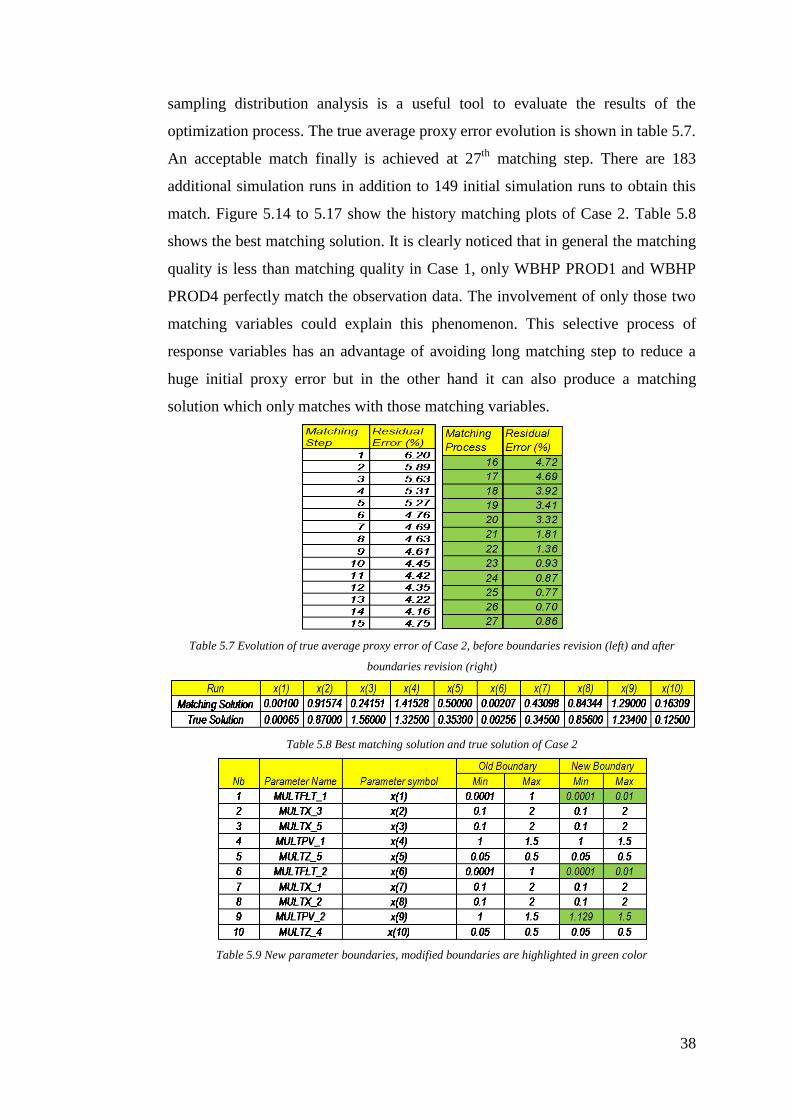
38

sampling distribution analysis is a useful tool to evaluate the results of the

optimization process. The true average proxy error evolution is shown in table 5.7.

An acceptable match finally is achieved at 27th

matching step. There are 183

additional simulation runs in addition to 149 initial simulation runs to obtain this

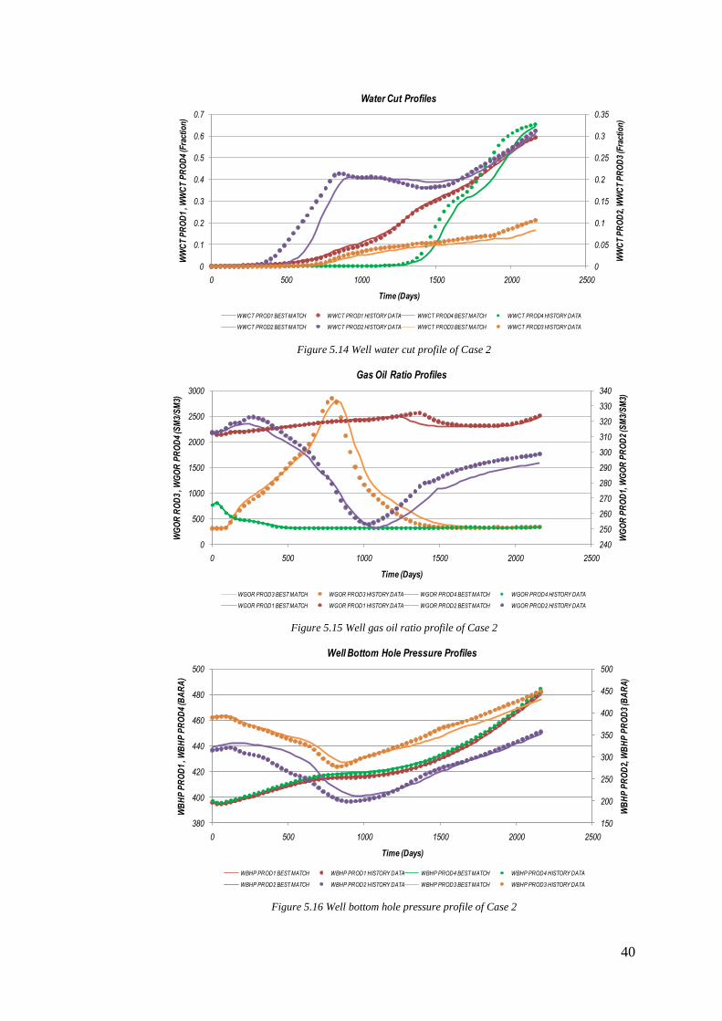
match. Figure 5.14 to 5.17 show the history matching plots of Case 2. Table 5.8

shows the best matching solution. It is clearly noticed that in general the matching

quality is less than matching quality in Case 1, only WBHP PROD1 and WBHP

PROD4 perfectly match the observation data. The involvement of only those two

matching variables could explain this phenomenon. This selective process of

response variables has an advantage of avoiding long matching step to reduce a

huge initial proxy error but in the other hand it can also produce a matching

solution which only matches with those matching variables.

Table 5.7 Evolution of true average proxy error of Case 2, before boundaries revision (left) and after

boundaries revision (right)

Table 5.8 Best matching solution and true solution of Case 2

Table 5.9 New parameter boundaries, modified boundaries are highlighted in green color

39

(a)

(b)

(c)

Figure 5.13 Sampling distribution of parameter x1 (a), x6 (b) and x9 (c)

0.00%

20.00%

40.00%

60.00%

80.00%

100.00%

120.00%

0

10

20

30

40

50

60

Fre

qu

ency

Bin

Sampling Distributions x(1)

Frequency

Cumulative %

0.00%

20.00%

40.00%

60.00%

80.00%

100.00%

120.00%

0

10

20

30

40

50

60

Fre

qu

ency

Bin

Sampling Distributions x(6)

Frequency

Cumulative %

0.00%

20.00%

40.00%

60.00%

80.00%

100.00%

120.00%

0

10

20

30

40

50

60

70

80

Fre

qu

en

cy

Bin

Sampling Distributions x(9)

Frequency

Cumulative %

40

Figure 5.14 Well water cut profile of Case 2

Figure 5.15 Well gas oil ratio profile of Case 2

Figure 5.16 Well bottom hole pressure profile of Case 2

0

0.05

0.1

0.15

0.2

0.25

0.3

0.35

0

0.1

0.2

0.3

0.4

0.5

0.6

0.7

0 500 1000 1500 2000 2500

WW

CT

PR

OD

2, W

WC

T P

RO

D3

(Fra

ctio

n)

WW

CT

PR

OD

1 , W

WC

T P

RO

D4

(Fra

ctio

n)

Time (Days)

Water Cut Profiles

WWCT PROD1 BEST MATCH WWCT PROD1 HISTORY DATA WWCT PROD4 BEST MATCH WWCT PROD4 HISTORY DATA

WWCT PROD2 BEST MATCH WWCT PROD2 HISTORY DATA WWCT PROD3 BEST MATCH WWCT PROD3 HISTORY DATA

240

250

260

270

280

290

300

310

320

330

340

0

500

1000

1500

2000

2500

3000

0 500 1000 1500 2000 2500

WG

OR

PR

OD

1, W

GO

R P

RO

D2

(SM

3/S

M3)

WG

OR

RO

D3

, WG

OR

PR

OD

4 (S

M3/

SM

3)

Time (Days)

Gas Oil Ratio Profiles

WGOR PROD3 BEST MATCH WGOR PROD3 HISTORY DATA WGOR PROD4 BEST MATCH WGOR PROD4 HISTORY DATA

WGOR PROD1 BEST MATCH WGOR PROD1 HISTORY DATA WGOR PROD2 BEST MATCH WGOR PROD2 HISTORY DATA

150

200

250

300

350

400

450

500

380

400

420

440

460

480

500

0 500 1000 1500 2000 2500

WB

HP

PR

OD

2, W

BH

P P

RO

D3

(BA

RA

)

WB

HP

PR

OD

1 , W

BH

P P

RO

D4

(BA

RA

)

Time (Days)

Well Bottom Hole Pressure Profiles

WBHP PROD1 BEST MATCH WBHP PROD1 HISTORY DATA WBHP PROD4 BEST MATCH WBHP PROD4 HISTORY DATA

WBHP PROD2 BEST MATCH WBHP PROD2 HISTORY DATA WBHP PROD3 BEST MATCH WBHP PROD3 HISTORY DATA

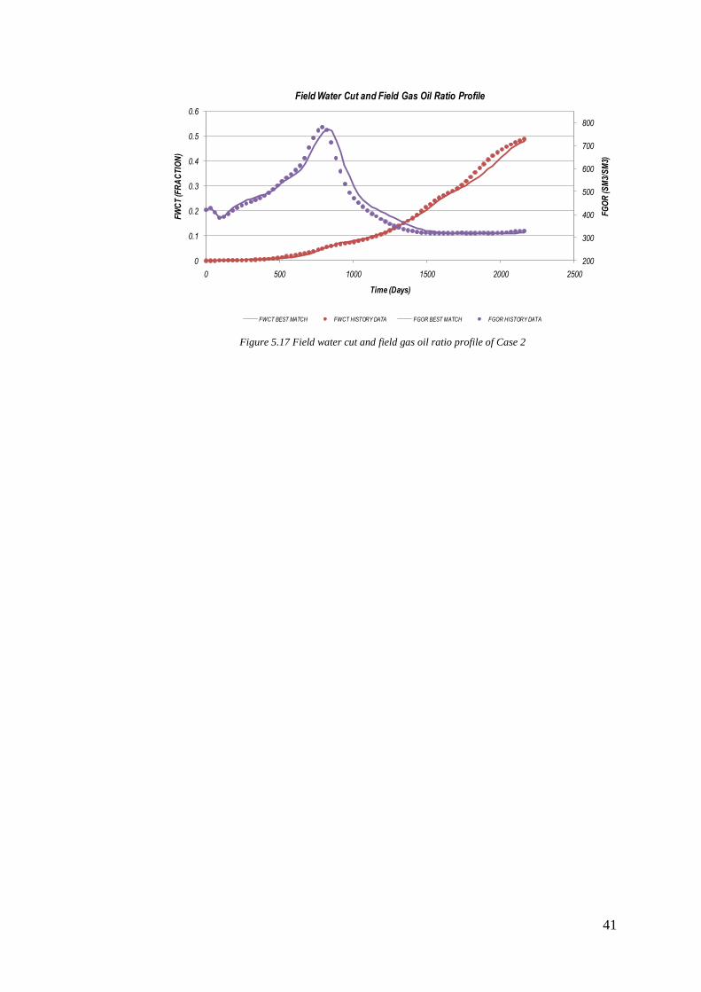
41

Figure 5.17 Field water cut and field gas oil ratio profile of Case 2

200

300

400

500

600

700

800

0

0.1

0.2

0.3

0.4

0.5

0.6

0 500 1000 1500 2000 2500

FG

OR

(SM

3/S

M3)

FW

CT

(FR

AC

TIO

N)

Time (Days)

Field Water Cut and Field Gas Oil Ratio Profile

FWCT BEST MATCH FWCT HISTORY DATA FGOR BEST MATCH FGOR HISTORY DATA

42

Chapter 6

Summary and Future Work

In this thesis, an investigation of computer assisted history matching is performed. A

comprehensive understanding of the subject is required to identify methodology limitations

so that improvements can be introduced in order to accelerate matching process. This study

also compares two types of proxy models e.g. kriging equation and second degree polynomial

equation which are used in the optimization process. Different global optimization algorithms

were also investigated in order to determine the best performance algorithm in solving history

matching problem.

6.1 Summary and Conclusions

a) The quality of proxy model plays an important role in assisted history matching.

Optimization algorithm is able to find the matching solution only if the proxy model

accurately predicts reservoir simulation responses.

b) Proxy model is initially built from a set of initial sample of experiments. The quality

of this initial proxy model depends on the sampling method. This study shows that

complete CCF design could generate a better proxy model than fractional CCF

design.

c) Different types of proxy model have different degree of accuracy in predicting

reservoir simulation. Kriging proxy model is able to predict reservoir simulation

more accurately than second degree polynomial equation.

d) The initial proxy model always has some error. This error must be minimized so that

the optimization algorithm is able to find a good match. This error can be reduced by

adding more experiments in the population which build the proxy model. The

additional experiments have to be located close to the matching or true solution so

that kriging proxy model can predict the response in that location more accurate.

These additional experiments are generated from the preceding optimization process.

This study proves that the inclusion of average proxy error in the objective function

is able to generate solutions which more improve the quality of proxy model.

e) Different values of average proxy error are inputted in the objective function in order

to have different solutions from the optimization. These values can be obtained from

43

average residual error analysis of secondary polynomial proxy model of initial

experiments.

f) From the investigation of different global optimization algorithms for the two cases,

it is concluded that direct search algorithm give the best performance in finding a

matching solution. Simulated annealing algorithm has slow convergence rate

therefore the maximum iteration is reached before it could find the matching

solution. Genetic algorithm is often trapped in the local minima. While global search

algorithm needs a longer time to find the matching solution.

g) Case 1 can be easily matched with only 7 matching steps and 34 additional reservoir

simulations in addition to the 43 initial experiments. The matching quality is almost

perfect. This is because of several reasons: first, the initial residual error is quite

small since complete CCF design is used to generate the initial experiments. Second,

all of the 12 response variables are included as matching variables.

h) Case 2 is more difficult to solve. There were 27 matching steps with 183 additional

simulations required to find an acceptable match. The matching quality is less than in

Case1. This is first because fractional CCF was used instead of complete CCF so that

the initial proxy model is not so accurate. Second, because the average quality of the

initial proxy model is bad, therefore we could only select response variables which

are accurately predicted by the proxy model.

i) Direct search algorithm in Case 2 could not explore all values of uncertain

parameters so that the reduction rate of residual error is slow. To overcome this

problem, sampling distribution analysis was conducted to redefine parameter

boundaries to force direct search algorithm to explore unexplored zones. Reduction

rate of residual error is significantly increased after the revision of boundary.

6.2 Future Work

a) Only two types of CCF design methods were investigated in this study. It will be

useful to investigate other design methods such as Box Behnken and Latin

Hypercube design.

b) Proxy model used in this study are second degree polynomial and ordinary kriging

equation. It will be of interest to study other types of proxy model such as universal

kriging, neural networks and Ensemble Kalman Filter.

c) A further improvement of direct search algorithm is also required so that it can

explore all values of the uncertain parameters.

44

d) In this study, the methodology was used to solve an artificial history matching

model. It will be of interest to use the same methodology to solve real history

matching problem.

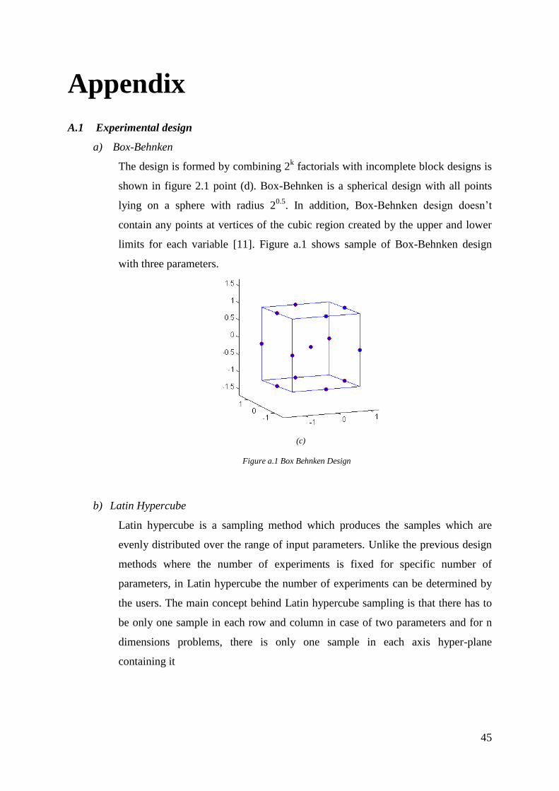
45

Appendix

A.1 Experimental design

a) Box-Behnken

The design is formed by combining 2k factorials with incomplete block designs is

shown in figure 2.1 point (d). Box-Behnken is a spherical design with all points

lying on a sphere with radius 20.5

. In addition, Box-Behnken design doesn’t

contain any points at vertices of the cubic region created by the upper and lower

limits for each variable [11]. Figure a.1 shows sample of Box-Behnken design

with three parameters.

(c)

Figure a.1 Box Behnken Design

b) Latin Hypercube

Latin hypercube is a sampling method which produces the samples which are

evenly distributed over the range of input parameters. Unlike the previous design

methods where the number of experiments is fixed for specific number of

parameters, in Latin hypercube the number of experiments can be determined by

the users. The main concept behind Latin hypercube sampling is that there has to

be only one sample in each row and column in case of two parameters and for n

dimensions problems, there is only one sample in each axis hyper-plane

containing it

46

Figure a.2 example of Latin hypercube design for two parameters with 5 sample points

The main advantageous of this design is that the number of experiments doesn’t

depend on the number of variables, so that this design is suitable for a problem

which involves many variables. Figure a.2 shows one example of Latin hypercube

design of two parameters with 5 sample points.

A.2 Kriging Proxy Model

The values of weighting factor of all the sampling points are determined with the

following equations:

……………………………………………………. (2)

………………………………….. (3)

…………….. (4)

………………. (5)

Based on the equations above, weighting factor is a function of two semi variogram

functions: first is semi variogram of non-sampling point and sampling points and

second, semi variogram between the sampling points.

γ1ΓW

)...,,.........,( ,21 nwwwW

T

nssssssγ )1),(....,),........(),(( 02010

1nj 1,nifor , 0

,...,2,1i 1,njfor , 1

,...,2,1j 1,nifor , 1

n1,2,.....,j ,n 1,2,....,ifor ),(

n

n

ss ji

Γ

47

Nomenclatures

AHM = Assisted History Matching

DOE = Design of Experiment

CCD = Central Composite Design

CCF = Cubic Centered Face

CCI = Cubic Centered Inscribed

CCC = Cubic Centered Circumscribed

Y = Response variables of polynomial equation

β = Parameters coefficient in polynomial equation

n = Number of parameters

Z = Response variables of kriging equation

s0 = Point of interest / un-sampled point

si = Sampled point i

wi = Weighting factor of sampled point si

Fobj = Objective function

T = Temperature

NewSol = New solution

CurSol = Current solution

p = Number of time steps

k = number of matching variables

VBA = Visual Basic Application

WWPT = Well water production total

WOPT = Well oil production total

WGPT = Well gas production total

FOPT = Field oil production total

FWPT = Field water production total

FGPT = Field gas production total

R2 = R squared

RS = Residual error

ycalc = Value of observe variables calculated from proxy model

ysim = Value of response variables obtained from simulation

yobs = Observation data

48

j = Average residual error of experiment j (%)

p = Average proxy error

Wi = Weighting factor of matching variable i

TolFun = Minimum changes of objective function

MaxIter = Maximum number of iterations

W = Matrix vector of weighting factor (kriging formula)

= Semi variogram

si-sj = Distance between sampled point i and point j

s0-sj = Distance between unsampled point and sampled point j

49

Bibliography

[1] C. Maschio and D.J. Schiozer. Development and application of methodology for

assisted history matching. Paper SPE 94882 prepared for SPE Latin American and

Caribbean Petroleum Engineering Conference held in Rio de Janeiro, 20 – 23 June,

2005.

[2] P. Ferraro and F.Verga. Use of evolutionary algorithm in single and multi-objective

optimization techniques for assisted history matching. This paper was presented at the

Offshore Mediterranean Conference and Exhibition in Ravenna, Italy, 25-27 March,

2009.

[3] Chaohui Chen, et al. Assisted history matching using three derivative-free

optimization algorithms. Paper SPE 154112 was prepared for presentation at the

EAGE incorporating SPE Europec held in Copenhagen, Denmark, 4-7 June, 2012.

[4] M. Cancelliere, et al. Benefits and limitations of assisted history matching. Paper SPE

146278 was prepared for presentation at the SPE Offshore Europe Oil and Gas

Conference and Exhibition held in Aberdeen, UK, 6-8 September, 2011.

[5] H. Cheng, K. Dehghani and T. Billiter. A structured approach for probabilistic-

assisted history matching using evolutionary algorithms: Tengiz field application.

Paper SPE 116212 was prepared for presentation at SPE ATCE held in Denver,

Colorado, USA, 21-24 September, 2008.

[6] R. Gupta, et al. History matching of field production using design of experiments. The

SPE paper 115685 was prepared for presentation at the SPE APOGCE held in Perth,

Australia, 20-22 October, 2008.

[7] S. Thomas and L. Nicolas. Using experimental design, assisted history matching tools

and Bayesian framework to get probabilistic production forecast. Paper SPE 113498

was prepared for presentation at SPE Europec and EAGE held in Rome, Italy, 9-12

June, 2008.

[8] L. den Boer et al. A new technique to achieve history matches using probabilistic

approach. Paper SPE 102871 was prepared for presentation at the SPE ATCE held in

San Antonio, Texas, USA, 24-27 September, 2006.

[9] Baoyan Li and F. Friedmann. Semi automatic resolution design for history matching.

SPE journal, 2007.

[10] M. C. Douglas. Design and Analysis of Experiments 6th Edition. Arizona, USA, 2005.

50

[11] Mathworks. Design of Experiments Statistics Toolbox. Users Guide, 2010.

[12] S. W. Timothy. Comparison of response surface and kriging models in the

multidisciplinary design of an aerospike nozzle. ICASE Report No. 98-16. Institute for

computer applications in science and engineering NASA Langley Research Center. Hampton

VA, 1998.

[13] C. Nicholas. Statistics lecture notes: ordinary kriging. University of California, LA,

2013.

[14] Mathworks. Global Optimization Toolbox. Users Guide, 2010.

[15] S.M. Sadiq and Y. Habib. Iterative Computer Algorithms with Applications in

Engineering. California, USA, 1999.

[16] RC. Chakraborty. Fundamental of genetic algorithm. AI course lecture

www.myreaders.info, 2010.

[17] Glover, F. A template for scatter search and path re-linking. Artificial Evolution (J.-

K. Hao, E.Lutton, E.Ronald, M.Schoenauer, D.Snyers, eds.). Lecture Notes in

Computer Science, 1363, Springer, Berlin/Heidelberg, 1998, pp. 13–54