Embed Size (px)
Citation preview

Exchange-rate regimes and economic recovery
A cross-sectional study of the growth
performance following the 2008 financial crisis
By: Sebastian Fristedt Supervisor: Xiang Lin
Södertörns University | Institution of Economics
Master Thesis 30 ECTS
Economics | Spring Semester 2017

ABSTRACT
This paper applies a cross-‐sectional regression analysis of 83 countries over the period 2009-‐11 in order to examine the role played by the exchange-‐rate regime in explaining how countries fared in terms of economic growth recovery following the recent financial crisis. After controlling for income categorization, regime classification, using alternative regime definitions, and accounting for various other determinants, the paper finds a significant relationship between the regime choice and the recovery performance, where those countries with more flexible arrangements fared better. These results were conditional on the regime classification scheme and the income level, implying an asymmetric effect of the regime during the recovery period between high and low income countries. The paper also finds that proxies for initial conditions as well as trade and financial channels were highly significant determinants of the growth performance during the recovery period.
KEYWORDS: Exchange-‐rate regime; Financial crisis; Global financial crisis, Economic growth recovery.

Table of Contents
Introduction ........................................................................................................................... 6 1.1 Background ................................................................................................................................. 6 1.2 Study objective ............................................................................................................................ 8 1.3 Problem statement ...................................................................................................................... 8 1.4 Methodology ............................................................................................................................... 8 1.5 Scope of study ........................................................................................................................... 10 1.6 Thesis structure ......................................................................................................................... 10
Definitions ............................................................................................................................ 12 2.1 Exchange-‐rate regime ................................................................................................................ 12 2.2 The impossible trinity principle ................................................................................................... 13 2.3 Exchange-‐rate Regime Classification ........................................................................................... 14
Previous Empirical Studies ..................................................................................................... 16
Theory ................................................................................................................................... 18 4.1 Growth framework .................................................................................................................... 18 4.2 Link between exchange-‐rate and monetary policy ....................................................................... 19
4.2.1 Long-‐run effects ........................................................................................................................ 20 4.2.2 Short-‐run effects ....................................................................................................................... 24
4.3 Link Between exchange-‐rate regime and economic growth and recovery ..................................... 27 4.3.1 Adjustment to shock ................................................................................................................. 28 4.3.2 Level of uncertainty ................................................................................................................... 31
4.3.3 Link to productivity ................................................................................................................. 32
Empirical Analysis .................................................................................................................. 34 5.1 Simple averages ......................................................................................................................... 34 5.2 Regression model ...................................................................................................................... 40 5.3 Regression analysis .................................................................................................................... 46
Conclusion ............................................................................................................................. 60
References ............................................................................................................................ 64
Appendix A: Data and summary statistics .............................................................................. 69
Appendix B: Normality, Heteroscedasticity, Multicollinearity and Linearity Checks ............... 76
Appendix C: Regression Result Tables and Robustness Tests ................................................. 82

Tables, Figures, and Equations
Tables
Table 1. Description of regression model variables 40 Table 2. Regression (1) results IMF Classification 46 Table 3. Regression (2) results Reinhart & Rogoff classification 56 Table 4. Regression (3) results with alternative peg definition 58 Table 5. Dataset: Classification, variables, and definitions 69 Table 6. Summary statistic 70 Table 7. Correlation Matrix 70 Table 8. Heteroscedasticity and Multicollinearity 79
Test statistics Table 9. Regression (1) results: IMF’s de facto classification scheme 82 Table 10. Regression (2) results: Reinhart & Rogoff de facto classification scheme 83 Table 11. Regression (3) results: Alternative peg definition IMF classification 84 Table 12. Regression (3) results: Alternative peg definition 85 Reinhart & Rogoff classification Figures Figure 1. Typology of Exchange-‐rate Regimes 13 Figure 2. Long-‐run Neutrality of Money 20 Figure 3. The Dutch Guilder’s Nominal and Real Exchange-‐rate 1970-‐2010 23 Figure 4. Monetary Expansion with Fixed Exchange-‐rates and 25 Perfect Capital Mobility Figure 5. Monetary Expansion with Flexible Exchange-‐rates and 26 Perfect Capital Mobility Figure 6. Growth Performance 35 Figure 7. Exchange-‐rate Regime Distribution 36 Figure 8. Growth Performance 37 Figure 9. Growth Performance Low-‐income Countries 38 Figure 10. Growth Performance High-‐income Countries 39 Figure 11. Rebound Effect 71 Figure 12. Foreign Exchange Reserves 71 Figure 13. Capital Formation (High-‐income) 72 Figure 14. Capital Formation (Low-‐income) 72 Figure 15. Current Account Balance 73 Figure 16. Trading Partner Recovery 73 Figure 17. Private Credit 74 Figure 18. Credit Restraint (Low-‐income) 74 Figure 19. Credit Restraint (High-‐income) 75 Figure 20. Kernel Density Test 76
Figure 21. pnorm Test 77 Figure 22. qnorm Test 78 Figure 23. Heteroscedasticity Diagnostic Plot 80 Figure 24. Linearity Check 81
Equations Equation 1. General Growth Framework Specification 18 Equation 2. Regression Model Equation 40

6
Introduction
1.1 Background
Almost one decade ago, the subprime mortgage market in the U.S. was approaching its absolute
breaking point and the severity of the situation was becoming undeniable. Short thereafter, the
investment bank Lehman Brothers filed for chapter 11 bankruptcy, constituting the largest
bankruptcy filling in U.S. history to date, triggering a full-‐blown global financial crisis only
comparable in magnitude to the great depression of the 1930s. The excessive and retrospectively
precarious risk taking that had preceded by banks acted to exacerbate the global impact as the
crisis rapidly spread from the U.S. to the rest of the world in an unprecedented manner.
As the crisis expanded, economists contemplated whether or not developing and emerging
market economies would be expected to follow the advanced market economies into a deep
recession-‐ as they quarreled how trade and finance has lead business cycles to become highly
synchronized-‐ or whether the impact of the recession could be mitigated by decoupling.
Pessimists questioned whether decoupling would be possible considering the current era of
globalization and financial interdependency. Optimist on the other hand recognized the ongoing
development of increasing trade activity between developing and emerging economies, as well
as the overall growth in domestic income and productivity as signs that the developing and
emerging economies were learning to spread their wings.
As the crisis deepened, most countries were primarily affected by external shocks to their
economies, largely through two main channels. The first was a substantial drawback of their total
exports, which for commodity producers lead to a significant drop in their terms of trade. The
second channel manifested as a sharp decline in the net flows of capital. The exposure was
however not fully homogenous among countries: where some were more open to trade than
others; some had large deficits in their current accounts and/or large short-‐term external debts,
whereas others had large foreign currency debts. The initial response also greatly varied among
countries, where some relied on monetary easing and some on fiscal expansion, some used their

7
accumulated reserves in order to uphold their exchange-‐rate, while others chose to let it adjust
accordingly.
Although it was largely the advanced economies and not the developing and emerging
economies that were at the epicenter of the recent crisis, their joint experience during and after
the crisis nevertheless is of upmost importance and may hold important lessons for the future,
whether it be in academic or policy circles. This paper addresses one such a lesson, namely the
one that concerns the choice of exchange-‐rate regime. The question being whether the
exchange-‐rate regime played a significant role in terms of how economies fared in this crisis,
particularly in terms of their output losses and economic recovery.
Economic growth theory and the literature on exchange-‐rate regimes suggests both direct and
indirect channels through which the choice of exchange-‐rate regime can affect the economic
growth of a country during the recovery period following the recent crisis. The direct channel
refers to the absorption ability of external shocks to the economy, whereby easing adjustment
should be associated with relatively smaller output losses and greater growth resilience. The
indirect channel arises through how it affects other key factors of economic growth, such as
investment, trade, financial sector development, and productivity. Although a popular
perception of the recent crisis was that It was weathered relatively better by those economies
with more flexible exchange-‐rate arrangements, it remains an empirical matter to estimate the
significance of the role that the choice of exchange-‐rate regime supposedly played in this matter.
This paper attempts to examine these issues by using a sample of 83 countries in a cross-‐sectional
regression analysis over the period 2009-‐11. In particular, an examination of the growth episodes
preceding and covering the crisis and recovery periods forms the basis for assessing whether or
not the choice of exchange-‐rate regime holds explanatory power over how these countries
performed in, and recovered from, the crisis in relation to one another. In addition to determining
the role that the exchange-‐rate regime played, the paper attempts to complement earlier
empirical work by identifying other important factors of economic performance and recovery
during and after the recent crisis and to determine whether these results are conditional to the

8
level of country development.
1.2 Study objective
The objective of this paper is to review the channels through which the choice of exchange-‐rate
regime theoretically can affect the economic growth performance during the recovery period
following a financial crisis and to empirically investigate the statistical validity of this relationship.
Additionally, to conduct an examination to specify whether there exists an asymmetric effect of
the impact that the choice of exchange-‐rate regime holds on the economic growth recovery
between high and low income countries. The foundation for the econometric specification used
in the empirical analysis will be derived from an extensive analysis of both general economic
growth theory and the literature on exchange-‐rate regimes. A secondary objective consists of
theoretically identifying and empirically estimating other important deterministic factors that
may have affected the recovery process.
1.3 Problem statement
The analysis of this paper will be formed by focusing on the following questions: (i) Did the choice
of exchange-‐rate regime play a deterministic role in the growth recovery following the financial
crisis of 2008? And, (ii) was the significance of this relationship symmetric across high and low
income countries?
1.4 Methodology
This paper will apply an econometric cross-‐sectional analysis consisting of 83 sampled countries
during the period 2009-‐11 in order to determine if the exchange-‐rate regime played a statistically
significant role in the economic recovery performance following the financial crisis of 2008, and
if the significance of this relationship suggest symmetry between high and low income countries.
The dependent variable used in the econometric analysis will be a measure of the average annual
per capita GDP growth for the period 2009-‐11. The explanatory variables of interest for this study
are the dummy variables that denote the choice of exchange-‐rate regime. The empirical analysis

9
uses the exchange-‐rate regime classification at the beginning of the recovery period provided by
(i) the IMF’s de facto classification published in 2009 Annual Report on Exchange Rate
Arrangements and Exchange Restrictions and (ii) the Reinhart & Rogoff (2011) de facto
classification scheme. The paper classifies the exchange-‐rate regime of the countries according
to the following definition, where (i) fixed exchange-‐rate regimes include hard pegs and
conventional pegs, (ii) flexible exchange-‐rate regimes include pure floats and managed floats,
and (iii) intermediate regimes include everything in between.
The empirical analysis controls for other deterministic factors of the economic growth recovery
by including variables that capture initial conditions, trade exposure and financial channels.
These variables include; the initial GDP per capita growth drop in 2008, the reserves to GDP ratio
in 2007, current account balance, trade (%GDP), capital formation (%GDP), private credit (%GDP),
FDI (%GDP). The estimated regression results will be tested using a broad set of robustness
checks including; grouping countries based on their level of income, alternative regime
classification scheme, alternative peg definitions, using a non-‐linear effect for the reserves, a
dummy for oil exporting countries, a dummy for countries with an inflation target, a dummy for
Latin American countries, and a proxy for fiscal policy. The macroeconomic variables used in the
empirical analysis are constructed from the World Bank’s databank and the IMF’s database.
Subsequently, appropriate specification models will be identified for the empirical analysis
according to a selection criterion based on the adjusted R2. These models will be subject to a
number of diagnostics test to assure that the estimates are unbiased and allow for valid
hypothesis testing. These tests include checking for normality, homoscedasticity,
multicollinearity and linearity. Both the model estimates and diagnostics tests will be carried out
using STATA as the program of choice.
The income categorization is based on the income classification system provided by the World
Bank that uses the World Bank Atlas method. Whereby low-‐income economies are those with a
GNI per capita that equals 0 < $1,045 or lower; middle-‐income economies with a GNI per capita
equal to $1,045 > $12,736; and high-‐income economies with a GNI per capita equal to X > $12,736

10
or higher. This method makes a distinction between higher-‐middle-‐income economies and lower-‐
middle-‐income economies at a GNI per capita equal to $4,125. For the purpose of this empirical
application the authors group these categories where high-‐income economies consist of higher-‐
middle-‐income to high-‐income economies and the low-‐income economies consists of lower-‐
middle-‐income to low-‐income economies.
1.5 Scope of study
The empirical analysis conducted within this study was confined to a sample of 83 observations
consisting of low and high income countries. The sample selection was drawn from the
population to include a fairly equal distribution of income levels, assuring that both income
groups be jointly represented by the outcome of the study. The observations were selected from
the list provided by the World Bank Organization of low and high income countries. Although the
construction of the sample was arbitrary and therefore renders no evident reason to believe that
the study suffers from sample selection bias, it is important to recognize that a different or larger
sample may lead to a significantly different conclusion than the one presented by this study. The
sample size is however sufficiently large to generate a credible regression and statistically
significant inferences. Extending the same logic to account for the selected recovery period,
model specification, and exchange-‐rate regime classification scheme, the authors admittedly
recognizes that the results may be conditional to the particular definition of recovery period,
model specification, and de facto exchange-‐rate regime classification scheme. Inferences made
on the relative significance of the choice of exchange-‐rate regime between low and high income
countries may also be conditional on how the income levels are defined.
1.6 Thesis structure
The opening section of this paper will provide the reader with several definitions and brief
discussions of a number of fundamental concepts that are necessary to fully comprehend in order
to effectively follow the subsequent sections. The authors strongly believe that this is a superior

11
approach as it makes the flow of the paper smoother and easier for the reader to follow. Less
contextually important concepts and notations are described in footnotes throughout the paper.
The following section consists of an overview of the existing empirical findings on the relationship
between the choice of exchange-‐rate regime and economic growth, in particular during recovery
periods. The aim of this section is to compare the outcome of previous studies and determine
how this paper positions itself and contribute to the existing body of research.
Further, a theoretical discussion will precede with the purpose of articulating the theoretical
arguments as to how the economic growth during the recovery period may be affected by the
choice of exchange-‐rate regime, taking both general economic growth theory and the literature
on exchange-‐rate regimes into consideration. We start by presenting an examination of the
general economic growth theory that has been adopted in order to account for the basis of the
model specification used in the econometric analysis. Next follows an extensive examination of
the long and short run relationship between monetary policy and economic growth, funneling
into a more detailed discussion of the specific theorized channels through which the choice of
exchange-‐rate regime can affect the economic growth recovery following a crisis.
The empirical analysis of the paper presides with a section of simple averages where the
economic performance of the sample countries before, during, and after the recent financial
crisis is illustrated and analyzed on the premise of how countries with different exchange-‐rate
regimes fared. This will be followed be a detailed description of the model specification of the
regression analysis, and a presentation of the explanatory variables and their theoretical
justification.
The concluding section contains a summation of the decisive results and estimates of this paper,
as well as a discussion on whether these results are consistent with the general economic growth
theory and the earlier empirical findings. Lastly, the authors will articulate their conclusive
remarks and formulate a closing answer to the problem statement.

12
Definitions
2.1 Exchange-‐rate regime
An exchange-‐rate regime is a structure implemented by the monetary authority of each country
in order to establish the exchange-‐rate of their domestic currency in the foreign-‐exchange
market. It is at the discretion of each country to autonomously adopt any exchange-‐rate regime
it believes to be optimal, and will typically do so, while not exclusively, by using monetary policy.
According to their degree of flexibility, the distinction amid these exchange-‐rate structures are
commonly made between fixed, intermediate and flexible regimes.
Fixed exchange-‐rate regime
A fixed exchange-‐rate, generally referred to as a peg, is well-‐defined as an exchange-‐rate regime
committed to maintain a fixed domestic currency, either to a foreign currency, a currency basket,
or any other tangible measure of value. The monetary authority determines the exchange-‐rate
and commits to buy or sell the domestic currency at a specific price. This predetermined price
level is maintained by the monetary authority through interest rate adjustments and/or official
intervention in the foreign-‐exchange market.
Intermediate exchange-‐rate regime
Crawling pegs, crawling bands, horizontal bands, and target zones are ordinarily referred to as
intermediate exchange-‐rate regimes. These regimes seek to combine stability and flexibility by
applying a rule-‐based system for adjustment of the par value. This is typically achieved either
through band of rates or as a function of inflation discrepancies. The IMF offers the following
description of a crawling peg -‐ “The currency is adjusted periodically in small amounts at a fixed
rate or in response to changes in selective quantitative indicators, such as past inflation
differentials vis-‐à-‐vis major trading partners, differentials between inflation target and expected
inflation in major trading partners.”

13
Flexible exchange-‐rate regime
A flexible exchange-‐rate regime allows the exchange-‐rate of the domestic currency to be
exclusively determined by the free market forces of supply and demand, rather then being
pegged or controlled by the monetary authority. There are two distinct types of flexible
exchange-‐rates, namely managed floats and pure floats. The former occurs when there is some
evidence of official intervention, while the later exist when there are no official intervention
activities.
Figure 1 Typology of exchange-‐rate regimes
Source: Source: Policonomics 2012©
2.2 The impossible trinity principle
The impossible trinity principle underlines the dilemma each country is faced with when deciding
upon which exchange-‐rate regime to adopt. The principle states that any one regime may only
inherit two of the following three characteristics simultaneously; free flow of capital, fixed
exchange-‐rate regime, and sovereign monetary policy (Findlay & O’Rourke 2007).
A key implication of the trilemma is the trade-‐off forced upon policy-‐makers; where an increase
in any one of the variables would induce a decline in the weighted average of the remaining two.

14
If a country were to opt for greater financial openness, for instance, it is faced with the choice of
sacrificing either exchange-‐rate stability or monetary policy independence contingent on the
particular policy preference (Aizenman et al 2013).
Under fixed exchange-‐rates, monetary authorities need to intervene in the foreign-‐exchange
market in order to maintain the exchange-‐rate at the determined equilibrium level. This type of
regime is typically adopted by countries characterized by; being open economies, small in size,
having concentrated trade, and harmonious inflation rate. Flexible regimes are on the other hand
generally adopted by countries that are characterized by; being closed economies, large in size,
having dispersed trade, and divergent inflation rate (Edison & Melvin 1990).
2.3 Exchange-‐rate Regime Classification
The value of a currency under a fixed exchange-‐rate regime would intuitively fluctuate no more
then within the narrow pre-‐established limits, where the monetary authority holds a formal
commitment to maintain its parity by intervening in the foreign-‐exchange market. The nature of
a floating currency then by contrast entails that the monetary authority of a flexible exchange-‐
rate regime holds no such a commitment. Naturally, it follows that the best description of an
exchange-‐rate regime should be the one that derives from what the stated intentions of the
monetary authority is. The system which categorizes countries based on what their monetary
authority allegedly claims their particular exchange-‐rate regime to be, asserts the basis of a de
jure classification scheme.
However, it has become common practice among various non-‐compliant governments to exploit
those benefits often times associated with a de jure fixed exchange-‐rate regime, for instance by
running an expansionary monetary policy which is inconsistent with their formal commitment of
maintaining the parity of the asserted peg. Similarly, a monetary authority that denies any kind
of formal commitment while regularly intervening in the foreign-‐exchange market, reasonably
can not be considered to hold a floating currency. The preceding cases illustrates how inferences
made solely on the basis of the de jure classification scheme may be vastly misleading and

15
inaccurate1. The apparent necessity of an alternative scheme that does not rely on the countries
own announcement, has lead to the formation of a de facto classification. A scheme following a
de facto classification categorizes countries according to the observed actual behavior of the
particular monetary authority in regards to their nominal exchange-‐rate, without taking heed of
whatever the governments’ own claim may or may not be.
The understanding of the discrepancy between the IMF’s de jure classification and de facto
classification is relatively well established by now. The phenomenon was first observed by Calvo
and Reinhart (2002). The behavior came to be referred to as the fear of floating and describes a
pattern of how countries seemingly acts to limit fluctuations in the external value of their
domestic currency. This behavior has ben found to be fairly widespread across both regions and
economic development levels. However, what is less known is that various de facto schemes are
in discord and uses different statistical approaches to ascertain the de facto regime
classification2.
1
The extent of this misalignment has been documented by Rose (2011), whereby an examination of existing datasets classifying the exchange-‐rate regime of countries revealed a significant level of divergence, where the de facto exchange-‐rate regime often times depart from their de jure classification. Eichengreen and Razo-‐Gracia (2013) reaffirms these findings and empirically demonstrates how disagreements in the level of flexibility among various de facto regimes are usual and non-‐random occurrences. This behavior was further found to be more common among EMEs and developing economies as opposed to advanced economies. The prevalence was also significantly higher in those economies with relatively developed financial markets, low foreign exchange reserves, and open capital accounts. 2 See, (Ghosh et al 2002); (Calvo & Reinhart 2002); (Reinhart & Rogoff 2004); (Levy-‐Yeyati & Sturzenegger 2005).

16
Previous Empirical Studies
Tsangarides (2012) examined the significance of the role that the choice of exchange-‐rate regime
holds in explaining how emerging economies performed during and after the recent global
financial crisis of 2008, in terms of growth resilience and output losses. The result indicated that
there was no difference in growth performance for fixed and flexible exchange-‐rate regimes
during the crisis. However, the analysis of the post-‐crisis period 2010-‐11, suggested that fixed
exchange-‐rate regimes fared far worse, and that the growth recovery appeared to be more rapid
among the economies with a flexible exchange-‐rate regime. The result highlights the asymmetric
effect of the exchange-‐rate regime during and post-‐crisis recovery.
In a sample of 75 developing countries during the period 1973-‐96, Broda (2002) found that the
responses to negative terms-‐of-‐trade shocks varied significantly across different exchange-‐rate
regimes. In response to these negative shocks, the study found that countries with fixed
exchange-‐rate regimes experienced significantly large declines in real GDP, while the real
exchange-‐rate slowly depreciated by means of aggregate fall in prices. Countries with flexible
exchange-‐rate regimes generally experience relatively small declines in real GDP and large and
instant real exchange-‐rate depreciations.
In a study based on 17 industrialized countries, Feldman (2011) examined the relationship
between exchange-‐rate volatility and unemployment. While controlling for other deterministic
factors of the level of unemployment, such as labor market institutions, business cycle
fluctuations, product market regulations, and the trade share of GDP, the results found a
significant relationship between the two and suggested that higher levels of volatility in the real
effective exchange-‐rate tend to lead to an increasing unemployment rate. The model predicted
that increasing exchange-‐rate volatility in period t leads to higher levels of unemployment in the
following periods, with obvious negative consequences for economic growth. These results are
consistent with the argued link between fixed exchange-‐rate regimes and output and/or
unemployment volatility (Mussa et al 2000), where flexible exchange-‐rate regimes result in lower
quantity volatilities, by facilitating real wage and price adjustments. However, speculative forces
17
have been shown to make the nominal exchange-‐rate its own source of volatility, thus suggesting
the possibility that a flexible exchange-‐rate regime in some cases can exacerbate the movements
of output and unemployment.
As far as the link between exchange-‐rate regime and economic growth goes, Ghosh et al (1995)
examined a sample of 145 countries over a period of 1960-‐90 and found that their may well be a
significant relationship between the choice of exchange-‐rate regime and the economic growth
rate in a country. The results suggest an indirect relationship, where the exchange-‐rate regime
effects the economic growth by stimulating increased levels of productivity and investment.
Higher investment was observed to be triggered by the increased policy confidence promoted by
pegged regimes, with an average of 2 percentage points of total GDP across the sample countries.
However, an important consideration is that a misallocation of resources in the economy can be
caused by a pegged rate set at the wrong level, and ultimately result in a slower productivity
growth compared to the countries whom had adopted a more flexible arrangement. This
relatively high rate of productivity growth observed under a flexible exchange-‐rate, somewhat,
reflects the relatively faster growth of external trade under these regimes. The study concluded
that the fastest growth was found under the intermediate regimes, with an average of over 2
percent annually.
Huang and Malhotra (2004) studied the relative importance of the choice of exchange-‐rate
regime in terms of economic growth, between advanced and developing countries. In a
comparison of the relationship between the choice of regime and the resulting economic growth
for advanced European and developing Asian countries, using the classification system of de facto
exchange-‐rate regime, the results uncovered two significant regularities. The choice of regime
did not indicate any significant effect on economic growth or of its variability among the
European countries, although the data, however, recognized slightly higher economic growth
rates to be associated with flexible exchange-‐rate regimes. The choice of exchange-‐rate regime
did however turn out to be a significant determinant of economic growth among the observed
Asian countries, where a non-‐linearly managed float was predicted to be the best choice. The
evidence discovered by this study suggests that the relative importance of the choice of

18
exchange-‐rate regime, in terms of economic growth, critically differs across levels of country
development.
Theory
4.1 Growth framework
The contemporary empirical growth literature draws on a general framework that specifies that
the growth rate (GR) of a country at time t is a function of state variables (SV) and control
variables (CV). This general specification of economic growth is consistent with both the
neoclassical and the endogenous models of growth.
Equation 1. General growth framework specification
𝐺𝑅# = 𝐹 𝑆𝑉# ; 𝐶𝑉# .
A neoclassical growth framework integrates the (SV) in order to capture the effect of the initial
position of the economy, whereas the (CV) are included to capture the alterations in in steady-‐
state levels across different countries. A fundamental prediction of this growth framework is the
idea of conditional convergence, meaning that growth rates tend to be higher when the relative
initial level of GDP per capita in relation to the steady-‐state position is lower. This prediction is
derived from the neoclassical assumption of diminishing returns to capita, where higher growth
rates and rate of returns are linked to countries that have a relatively low initial capital per labor
ratio, in comparison to their long-‐run ratio. The convergence is, however, conditional due to the
interdependency of the steady-‐state levels of output and capital per laborer and the growth rate
of the population, the rate of saving, and the general position of the production function
properties that differ across countries (Barro & Sala-‐i-‐Martin 2004).
An endogenous growth framework, on the other hand, always assumes an economy to be in its
long-‐run equilibrium steady-‐state. Instead, the independent variables are used to capture the
different levels of steady-‐state growth rates across different countries. Economic growth is thus

19
emphasized by the endogenous growth framework as being the endogenous outcome of an
economy, and not the result of any external forces (Barro & Sala-‐i-‐Martin 2004).
It follows that this specification is consistent with both the neoclassical growth framework, in as
much as it explains the determinants of differential transitional growth rates among countries as
they converge towards their long-‐run steady-‐states, and the endogenous growth framework, as
the user is allowed to determine the differences of the steady-‐state growth rates across
countries. It is therefore appropriate to make use of this growth specification as a basis for
empirical analysis, since it is in accordance to general growth theory and at the same time
provides a comprehensive foundation that effectively accommodates both the neoclassical and
endogenous growth models. Consequently, the validity of this specification is solid regardless to
whether the user adopts the assumption of the considered country to be in its long-‐run steady-‐
state or not. It should, however, be noted that there is a major drawback of using such a general
specification. Due to the fact that the theory of economic growth does not provide any clear
consensus of which specific control variables to include, although this choice may be relatively
self-‐evident, it becomes problematic to translate such a framework into a specification that can
be empirically tested (Barro & Sala-‐i-‐Martin 2004).
4.2 Link between exchange-‐rate and monetary policy
The exchange-‐rate determines the price at which the domestic currency is valued in terms of
foreign currencies. The exchange-‐rate is of great practical importance to those market agents
involved in international transactions, whether it be for investment or trade. In addition, the
exchange-‐rate also has a principal position in monetary policy, where it may be used as an
instrument, a target, or an indicator-‐ depending on the particular framework of monetary policy
(Latter 1996).
It is important to separate the short and long run effects when evaluating the relationship
between the exchange-‐rate and monetary policy (Baldwin & Wyplosz 2004). While changes to
the exchange-‐rate may have an impact on the real economy and on the balance of payments in

20
the sort-‐run, due to the stickiness of prices (Parkin 2012), macroeconomic theory states that
money is neutral in the long-‐run, meaning that any effort to over stimulate an economy through
either expansionary monetary policy or currency devaluation will only result in a higher inflation
rate, short of any real economic growth (Goldstein 2002).
4.2.1 Long-‐run effects
Neutrality of money
The neutrality of money is the principle that describes how any change in nominal variables, such
as the exchange-‐rate, has no effect on the real variables in the economy, such as real GDP,
employment, and real consumption. The reason is that these nominal changes will be absorbed
by the proportional changes in the price level of the economy in the long-‐run. The implications
are that the monetary authority theoretically holds no ability to affect the real economy thought
monetary policy in the long-‐run (Patinkin 1989).
Figure 2. Long-‐run Neutrality of Money
Source: Baldwin & Wyplosz 2006

21
The graphical depiction of the theory illustrates the aggregate supply (AS) and aggregate demand
(AD) and how they convey the relationship between the inflation rate, as measured on the
vertical axis, and the change of the output gap measured on the horizontal axis. The negative
slop of the AD-‐curve illustrates how increased inflation erodes the purchasing power of money
and by doing so discouraging investment and consumption. The short-‐run AS curve illustrates
that monetary policy matters in the short-‐run and can be channeled into real economic activity
via the interest rate, credit expansion, stock market and exchange-‐rate.
However, the long-‐run AS-‐curve depicts a different story, namely how these changes in the
nominal variables has no real economic effects in the long-‐run, and will be offset by proportional
changes in the price level. If the price of consumer goods were to rise faster than wages, it would
mean that the purchasing power of wages would gradually decline. Eventually, workers would
become dissatisfied and begin to bargain for wage increases. Similarly, were we to experience
wages rising faster than prices, firms would be facing rapidly increasing cost and would sooner
or later be forced to increase their prices (Baldwin & Wyplosz 2006).
Purchasing Power Parity (PPP)
In the long-‐run, the PPP can be used to illustrate a second implication of the relationship between
the exchange-‐rate and the neutrality of money. The PPP can be seen as an artificial currency and
a statistical indicator that represents the disparities in national price-‐levels that are unaccounted
for by exchange-‐rates. The relative prices of a representative and comparable basket of goods
and services are used as a basis for this measurement among countries (Jovanovic 2013).
The PPP principle builds on the vital distinction between nominal and real exchange-‐rates. Where
the nominal exchange-‐rate is the value of foreign currency expressed in terms of the domestic
currency and the real exchange-‐rate is the the cost of foreign goods and services expressed in
terms of domestic goods and services. The real exchange-‐rate is the nominal exchange-‐rate
adjusted by the domestic and foreign price-‐levels, and is thus a measure of a countries relative
competitiveness (Burda & Wyplosz 2012).

22
𝑅𝑒𝑎𝑙 𝐸𝑥𝑐ℎ𝑎𝑛𝑔𝑒 𝑟𝑎𝑡𝑒 = 𝑁𝑜𝑚𝑖𝑛𝑎𝑙 𝐸𝑥𝑐ℎ𝑎𝑛𝑔𝑒 𝑟𝑎𝑡𝑒 ∗ 𝐷𝑜𝑚𝑒𝑠𝑡𝑖𝑐 𝑝𝑟𝑖𝑐𝑒 𝑙𝑒𝑣𝑒𝑙
𝐹𝑜𝑟𝑒𝑖𝑔𝑛 𝑝𝑟𝑖𝑐𝑒 𝑙𝑒𝑣𝑒𝑙
The principle suggests that alterations in the nominal exchange-‐rate between two currencies will
be equivalent to the difference in the inflation rate between these same countries. The difference
between domestic and foreign inflation rate is termed as the inflation differential (Husted &
Melvin 2012).
𝐸𝑥𝑐ℎ𝑎𝑛𝑔𝑒 𝑟𝑎𝑡𝑒 𝑎𝑝𝑝𝑟𝑒𝑐𝑖𝑎𝑡𝑖𝑜𝑛 = 𝐹𝑜𝑟𝑒𝑖𝑔𝑛 𝑖𝑛𝑓𝑙𝑎𝑡𝑖𝑜𝑛 𝑟𝑎𝑡𝑒 − 𝐷𝑜𝑚𝑒𝑠𝑡𝑖𝑐 𝑖𝑛𝑓𝑙𝑎𝑡𝑖𝑜𝑛 𝑟𝑎𝑡𝑒BCDEF#GHC IGDDJKJC#GFE
When the domestic country experiences a real exchange-‐rate appreciation, their goods and
services will become relatively more expensive compared to the foreign country and their
competitiveness will consequently fall. An appreciation in the real exchange-‐rate will follow from
an appreciation of the nominal exchange-‐rate and/or if the relative domestic prices are rising
faster than that of foreign prices. Conversely, a depreciation in the domestic real exchange-‐rate
will mean a relative increase in their level of competitiveness (Burda & Wyplosz 2012).
However, this effect can not go on forever and this is where the principle of neutrality becomes
important. In the long-‐run the nominal exchange-‐rate will adjust towards restoring the relative
competitiveness. This change will be equivalent to the full amount of the accumulated inflation
differential, and will thus nullify the short-‐run change in relative competitiveness. This
assumption implies that nominal variables can not affect real variables in the long-‐run, and that
countries must retain its competitiveness in the long-‐run. In the long-‐run, the real exchange-‐rate
should thus be unaffected by short-‐run fluctuations in nominal exchange-‐rates and relative price
levels. The PPP thereby asserts that the real-‐exchange rate is constant in the long-‐run (Burda &
Wyplosz 2012).
23
Δ𝜎𝜎
𝐶ℎ𝑎𝑛𝑔𝑒 𝑖𝑛 𝑟𝑒𝑎𝑙 𝐸𝑥𝑐ℎ𝑎𝑛𝑔𝑒 𝑟𝑎𝑡𝑒
= Δ𝑆𝑆
𝐶ℎ𝑎𝑛𝑔𝑒 𝑖𝑛 𝑛𝑜𝑚𝑖𝑛𝑎𝑙 𝐸𝑥𝑐ℎ𝑛𝑎𝑔𝑒 𝑟𝑎𝑡𝑒
+ 𝜋 − 𝜋 ∗
𝐼𝑛𝑓𝑙𝑎𝑡𝑖𝑜𝑛 𝑑𝑖𝑓𝑓𝑒𝑟𝑒𝑛𝑡𝑖𝑎𝑙= 0.
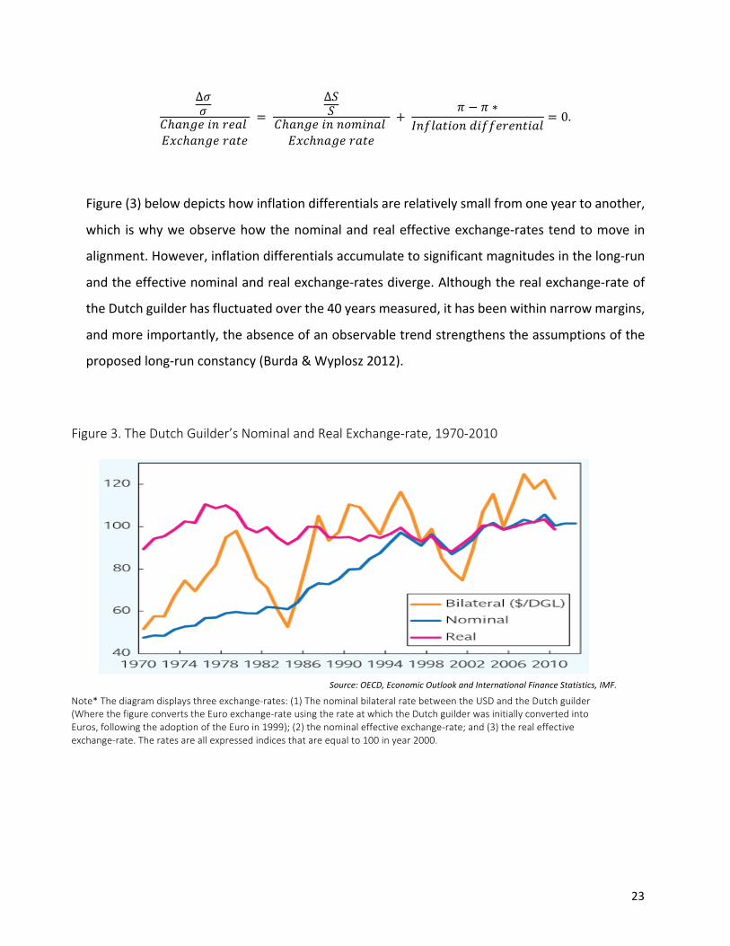
Figure (3) below depicts how inflation differentials are relatively small from one year to another,
which is why we observe how the nominal and real effective exchange-‐rates tend to move in
alignment. However, inflation differentials accumulate to significant magnitudes in the long-‐run
and the effective nominal and real exchange-‐rates diverge. Although the real exchange-‐rate of
the Dutch guilder has fluctuated over the 40 years measured, it has been within narrow margins,
and more importantly, the absence of an observable trend strengthens the assumptions of the
proposed long-‐run constancy (Burda & Wyplosz 2012).
Figure 3. The Dutch Guilder’s Nominal and Real Exchange-‐rate, 1970-‐2010
Source: OECD, Economic Outlook and International Finance Statistics, IMF.
Note* The diagram displays three exchange-‐rates: (1) The nominal bilateral rate between the USD and the Dutch guilder (Where the figure converts the Euro exchange-‐rate using the rate at which the Dutch guilder was initially converted into Euros, following the adoption of the Euro in 1999); (2) the nominal effective exchange-‐rate; and (3) the real effective exchange-‐rate. The rates are all expressed indices that are equal to 100 in year 2000.
24
4.2.2 Short-‐run effects
Interest rates
The preceding section concluded that, although the neutrality of money principle asserts that
monetary policy does not have a long-‐run effect on the real economy, it can have an impact in
the short-‐run. An expansive monetary policy will put downward pressure on the interest rate,
making firm investment more attractive. The result of this monetary intervention will be higher
aggregate spending, lower unemployment, and GDP growth. The now relatively high foreign
interest rates will make foreign financial assets more attractive, which under a floating exchange-‐
rate will yield a depreciation in the domestic nominal exchange-‐rate. This will cause a real
depreciation, stimulate the export sector and by doing so increase the relative competitiveness
of the home country (Baldwin & Wyplosz 2004).
The situation changes when considering the same scenario under a fixed exchange-‐rate regime.
In a state of rising prices and costs, the real exchange-‐rate will appreciate, which will have a
hampering effect on the country’s competitiveness and lead to a trade balance deficit. This could
be counteracted by lowering the interest rate as previously discussed, however, since the country
has committed to a fixed exchange-‐rate policy, their monetary authority will need to intervene
with other measures. The exchange-‐rate appreciation will be mitigated by increasing foreign
reserves and selling the domestic currency, thereby increasing the supply of money.
The theory of sterilization permits the monetary authority under a fixed exchange-‐rate regime to
exercise some control over its own supply of money, as long as foreign and domestic financial
assets are imperfect substitutes. However, if the financial assets were to be perfect substitutes,
they would have to yield the same rate of return to all investors. With the fixed exchange-‐rate,
this implies that the domestic interest rate will be equal to the foreign interest rate, because with
perfect capital mobility, any deviation of the domestic interest rate from the foreign interest rate
would encourage investors to only hold the assets yielding the highest rate of return adjusted to
the relative risk. This means that the monetary authority under a fixed exchange-‐rate regime is

25
not able to control both the money stock and the exchange-‐rate, and is thus left a small room for
sovereign monetary policy (Husted & Melvin 2012).
Figure 4. Monetary Expansion with Fixed Exchange-‐rates and Perfect Capital Mobility
Source: International Economics Eighth Edition 2010.
With perfect capital mobility the balance of payment curve BP is a flat line at the domestic
interest rate I, which is equivalent to foreign interest rate iF under the assumption of perfect
capital mobility. If the monetary authority were to expand the money supply, the LM-‐curve would
consequently shift from LM à LM’. The IS-‐LM equilibrium then moves from e à e’, and although
e’ results in a new equilibrium in the money and goods markets, there will be a large outflow of
capital and a large official settlements of balance deficit. This will put downward pressure on the
domestic currency in the foreign-‐exchange market, and in order to maintain the fixed exchange-‐
rate, the monetary authority must intervene by selling foreign exchange reserve and buying the
domestic currency. This intervention on the foreign-‐exchange market will lead to a decline in the
supply of money and shift the LM-‐curve back to LM’ à LM, and by doing so restoring the initial
IS-‐LM equilibrium at e. This effect would be instantaneous with perfect capital mobility and no
deviation from e would actually be observed. This concludes that any effort to change the money
supply by shifting the LM-‐curve would cause just the opposite effect on the interest rate and the
intervention activity (Husted & Melvin 2012).

26
Figure (5) illustrates the effect of an expansionary monetary policy under a flexible exchange-‐
rate regime. The important difference from the analysis made above in figure (4) is that under a
flexible regime, the monetary authority is not obliged to intervene in the foreign-‐exchange
market to maintain a particular exchange-‐rate parity. In the absence of intervention, the official
settlements balance will always equal zero. In addition, it allows the supply of money to change
to any level desired by the monetary authority, and it is this autonomy of monetary policy that is
one of the main virtues of a flexible exchange-‐rate regime, as often argued by its proponents
(Husted & Melvin 2012).
A monetary expansion will increase the supply of money and shift the LM-‐curve rightward to LM’.
The corresponding income and interest rate at point e’ would yield a state of equilibrium in the
money and goods markets, but would also lead to a higher deficit in the capital account as an
effect of the domestic interest rate I being lower then the foreign interest rate iF at this point.
The official settlement deficit is averted by following adjustment of the flexible exchange-‐rate to
a level that restores the equilibrium at point e’’. Specifically, the pressure created by the official
settlements deficit would trigger a depreciation in the domestic currency, and the IS-‐curve would
shift right towards IS’, as the domestic net-‐exports increase. At the new equilibrium e’’, income
is higher and the domestic interest rate I is equal to the foreign interest if. This concludes that
the level of income can be changed with monetary policy under a flexible exchange-‐rate regime.
Figure 5. Monetary Expansion with Flexible Exchange-‐rates and Perfect Capital Mobility
Source: International Economics Eighth Edition 2010

27
As the exchange-‐rate is adjusted to restore the balance of payments equilibrium, the monetary
authority is able to choose its monetary policy autonomously of the policies preferred by other
countries (Husted & Melvin 2012).
4.3 Link Between exchange-‐rate regime and economic growth and recovery
The natural-‐rate hypothesis implies that macroeconomic policy can only hope to achieve price
stability in the medium-‐run. The implications of this principle in terms of exchange-‐rate policy, is
that the nominal exchange-‐rate as a policy tool, is incapable of keeping unemployment rates
below its natural level in any sustainable manner (Goldstein 2002). This means that any attempt
of the monetary authority to over stimulate the economy, either by conducting an expansionary
monetary policy or by devaluating its domestic currency, will only result in higher inflation rate,
without any increase in the real economic variables (Barro & Gordon 1983).
Hence, as a nominal variable, the exchange-‐rate-‐regime might not be a causal determinant of the
long-‐run economic growth. However, monetary policy can have an impact on economic growth
in the short-‐run, and thus be a conceivable deterministic factor of the economic growth recovery
following a financial crisis (Baldwin & Wyplosz 2004). While there indeed is no definite theoretical
evidence that explains which exchange-‐rate regime is more apt to stimulate post-‐crisis economic
growth, the literature on exchange-‐rate regimes argues the existence of both direct and indirect
channels, through which the choice of exchange-‐rate regime theoretically may affect economic
growth. These channels include the regimes effect on: i) shock adjustment; ii) level of uncertainty;
and iii) financial sector development (Bailliu et al 2003).

28
4.3.1 Adjustment to shock
Most relevant for the topic of this paper is the direct channel through which the choice of
exchange-‐rate regime can effect the post-‐crisis economic growth recovery. The literature on
exchange-‐rate regimes has emphasized how the adjustment process of an economy following a
shock can differ greatly in regards to the nature of the considered exchange-‐rate regime. For
instance, it has been argued that although the long-‐run equilibrium is equal among flexible and
fixed exchange-‐rate regimes, the adjustment process and movement towards that equilibrium
will not be identical (Mundell 1968).
Bailliu et al (2003) argues that the effect is channeled through the exchange-‐rate regimes’
influence on economic growth by ‘’dampening or amplifying the impact and adjustment to
economic shocks’’. The mitigation of business cycles has indeed been revealed to have a positive
impact on the growth rate of an economy. For instance, a model developed by Barlevy (2001)
effectively demonstrates how mitigating the cyclical fluctuations increases economic growth by
raising the average level of investment and by lessening its volatility. Similarly, Kneller and Young
(2001) found a significant negative relationship between the variability of output and the long-‐
run economic growth in their sample survey of 24 OECD countries, covering the period from
1961-‐97.
It has been argued that flexible exchange-‐rate regimes promote higher economic growth, since
such an arrangement will allow an economy, characterized by nominal rigidities, easy and fast
adaptation and absorption to economic shocks, as it allows the movement of exchange-‐rates to
act as shock-‐absorbers. Thus, given that the economy is operating close to capacity on average,
one would expect relatively higher growth when the adjustment process to economic shocks is
smoother (Bailliu et al 2003).
Similarly, Friedman (1953) claims that flexible exchange-‐rate regimes are able to absorb external
shocks; as apposed to a stringent exchange-‐rate target, where the adjustment is directed through
the change in the relative prices. Nonetheless, in a world of Keynesian prices, characterized as
distributing a sort of stickiness, this process of adjustment is sluggish, and thus ultimately

29
impairing the economic growth as an effect of the excessive burden created in the economy.
Furthermore, in an environment of perfect (or at least high) capital mobility, needed changes in
the interest rate produce increasingly high costs for the economy, in their struggle to defend its
peg during a currency attack. In regards to this, Fisher (2001) argues that the free movement of
capital across borders in modern times has made fixed exchange-‐rate regimes unsustainable,
often causing severe recessions in times of crisis.
Some would oppose, however, the notion of flexible exchange-‐rate regimes being able to absorb
external shocks to the economy. For instance, Levy-‐Yeyati and Sturzenegger (2002) explain that
such circumstances may instead stimulate protectionistic behavior and distorted prices, causing
a misallocation of resources in the economy. However, the cause of this effect is ambiguous, and
Nilsson and Nilsson (2000) argue that the protectionistic behavior observed under flexible
exchange-‐rate regimes in fact could be promoted by the increasing exchange-‐rate volatility under
such circumstances.
Moreover, there are some parts of the literature that claims that flexible exchange-‐rate regimes
in fact are more prone to economic shocks. They argue, that compared to a fixed exchange-‐rate
regime, the exchange-‐rate volatility introduced under a flexible regime adds an additional source
of shocks to the economy that may amplify the effects of the business cycle and actually dampen
the growth following the shock. This effect could be exacerbated in economies with relatively
weak or underdeveloped financial markets, since they will have issues with accommodating
significant exchange-‐rate movements under a flexible arrangement (Bailliu et al 2003).
In addition, the independent monetary policy that is allowed under a flexible exchange-‐rate
regime, provides the economy with additional means to accommodate both domestic and
foreign economic shocks. Some would contend, however, that this argument only is valid for
those economies that have a certain monetary policy credibility. Indeed, some economies has
shown that by fixing the exchange-‐rate to a hard currency rather then attempting to conduct an
independent monetary policy has resulted in a much smoother business cycle (Bailliu et al 2003).
Flexible exchange-‐rate regimes in Latin America has for instance been found to not having
30
promoted a more stabilizing monetary policy, but instead tending to be more pro cyclical
(Hausmann et al. 1999).
The comparison has up until now focused on flexible versus fixed exchange-‐rate regimes,
however, there are numerous other regime options positioned in between these two polar
extremes; often referred to as intermediate exchange-‐rate regimes. A common view is that
increasing capital mobility has lead intermediate exchange-‐rate regimes to become
unsustainable arrangements for economies. The intuition of this argument is that intermediate
exchange-‐rate regimes supposedly lacks credibility and therefore are more likely to be the
subject to speculative currency attacks (Bailliu et al 2003).
It has been noted that intermediate exchange-‐rate regimes often tend to be more difficult for
foreign investors to monitor than pure floats or hard pegs (Frankel et al. 2001). Others, argue
that economies that choose an intermediate exchange-‐rate regime fundamentally are more
susceptible to economic crises. The reason is that such an arrangement does not provide
sufficient incentives for neither private market agents or policy-‐makers to assume actions that
would increase the resiliency of the economy to economic crises (Eichengreen 2000; Glick 2000).
However, there are those who claim that intermediate exchange-‐rate regimes are a viable
option, and even more so when considering the effects for emerging economies. The virtue of an
intermediate arrangement is thought of being the trade-‐off it admits between flexibility and
credibility for countries in their choice of exchange-‐rate regime, or for those countries that are
transitioning to a flexible exchange-‐rate regime or monetary union (Williamson 2000).
It is nevertheless important to take into consideration that the creation of all intermediate
exchange-‐rate regimes is heterogeneous, thus making it very important to distinguish between
credible intermediate exchange-‐rate regimes and those where credibility is scarce (Bailliu et al
2003). This reinforces the need to control for differentiated exchange-‐rate regime classification
schemes when assessing what type of monetary policy framework that is currently being
employed by different countries.

31
4.3.2 Level of uncertainty
Proponents of fixed exchange-‐rate regimes often argue how such an arrangement reduces the
level of uncertainty and lowers the interest rate variability, and thereby generating an economic
environment suitable for both trade and investment. A fixed exchange-‐rate is thought to
promote more rapid output growth in the medium to long run due to the greater level of
openness to international trade it imposes (Petreski 2009). This idea is shared by Gylfason (2000)
who argues that it is the relative stability a credible peg imposes that acts to stimulate
international trade and investment, accordingly invigorating increased economic efficiency and
growth.
Furthermore, De Grauwe and Schnabl (2004) argues that there are two contributing factors that
may trigger relatively higher levels of output growth under a fixed exchange-‐rate regime. Firstly,
international trade and division of labor may be induced by the absence of exchange-‐rate risk,
and secondly, that the credibility imposed by a credible fixed exchange-‐rate will lead to a
reduction in the risk premium of a countries interest rate, where lower interest rates are
associated with higher investment and consumption levels.
Other strains of the exchange-‐rate literature identify two channels through which a flexible
exchange-‐rate regime may hamper the volume of international trade and investment. The first
way is related to the relatively high level of exchange-‐rate uncertainty it imposes for agents
conducting international trade and investment, and a second way is due to the creation of trade
barriers that are formed as a response to the relatively high levels of exchange-‐rate volatility
under such arrangements (Brada & Mendez 1988).
The former discussion adheres to the notion that the level of uncertainty increases when a
flexible exchange-‐rate arrangement is adopted, and extends the argument to conclude that it is
a stable macroeconomic environment that primarily stimulates international trade and
investment. However, Viaene and de Vries (1992) scrutinizes this general assumption, and
questions whether the level of exchange-‐rate uncertainty is unambiguously negatively correlated
to international trade and investment. They argue that market agents’ incentives for conducting

32
international trade and investment in fact can be augmented by intensified exchange-‐rate
fluctuations, depending on their particular level of risk acceptance. It follows that there may well
be a positive correlation between international trade and investment and increasing levels of
exchange-‐rate uncertainty, as long as the levels of risk acceptance are sufficiently high.
An important proponent of this perception is that agents are provided with efficient tools, such
as forward markets, for hedging the associated exchange-‐rate risk, instruments that are not
always available, particularly in developing markets (Bailliu et al 2003). Bordo and Flandreau
(2001) analysis of the post-‐Bretton Woods period support this notion, where they found evidence
that suggested that those countries with relatively more developed financial systems tended to
have more flexible exchange-‐rate arrangements.
4.3.3 Link to productivity
The Solow growth model shows how output growth either can be a result of an increase in one
of the factors of production and/or of the total factor productivity. Therefore, if the pervious
arguments made by proponents of fixed exchange-‐rate regimes are true, namely, that the
existence of an exchange-‐rate target acts to stimulate international trade and investment, then
it should also be true that lower levels of output under such an arrangement must be associated
with lower productivity growth. This theoretical relationship becomes even more pronounced in
developing and emerging markets where there is an overall lack of well-‐developed financial
markets (Petreski 2009).
Consequently, given the overall underdevelopment of financial markets, a country operating
under a fixed exchange-‐rate regime may experience how aggregate external shocks channel into
real economic activity. This will ultimately trigger a spiral where an increasing number of firms
experience a credit constraint, with obvious ripple effects on the aggregate economic growth
(Aghion et al 2005).
Producing firms have to decide whether to invest in short-‐term capital or in productivity
enhancing long-‐term venture. The latter strategy typically requires a relatively higher demand

33
for liquidity in order to allow maneuvering around idiosyncratic liquidity shocks over the medium-‐
run, which are often caused by external aggregate shocks to the economy. Underdeveloped
credit markets are unfortunately unable to supply the domestic firms with the needed liquidity
and only the firms, who’s profits are sufficiently large may borrow to cover their liquidity cost.
The external aggregate shock will cause the profitability of many firms to fall, and this will thus
reduce the likelihood that any of their liquidity needs can be filled. The overall impact is that a
large portion of the potential productivity enhancing investments will be unfulfilled. Therefore,
the main implication of this theory is that firms operating in an economic environment with a
perfect (or at least well-‐developed) financial market are in a better position to maneuver the
aggregate shocks, thus, stimulating firms to peruse these investments which theoretically should
promote economic growth (Petreski 2009).
34
Empirical Analysis
5.1 Simple averages
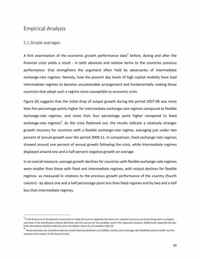
A first examination of the economic growth performance data3 before, during and after the
financial crisis yields a result -‐ in both absolute and relative terms to the countries previous
performance-‐ that strengthens the argument often held by adversaries of intermediate
exchange-‐rate regimes. Namely, how the present day levels of high capital mobility have lead
intermediate regimes to become unsustainable arrangement and fundamentally making those
countries that adopt such a regime more susceptible to economic crisis.
Figure (6) suggests that the initial drop of output growth during the period 2007-‐08 was more
than five percentage points higher for intermediate exchange-‐rate regimes compared to flexible
exchange-‐rate regimes, and more than four percentage point higher compared to fixed
exchange-‐rate regimes4. As the crisis flattened out, the results indicate a relatively stronger
growth recovery for countries with a flexible exchange-‐rate regime, averaging just under two
percent of annual growth over the period 2009-‐11. In comparison, fixed exchange-‐rate regimes
showed around one percent of annual growth following the crisis, while intermediate regimes
displayed around one and a half percent negative growth on average.
In an overall measure, average growth declines for countries with flexible exchange-‐rate regimes
were smaller than those with fixed and intermediate regimes, with output declines for flexible
regimes-‐ as measured in relations to the previous growth performance of the country (fourth
column) -‐ by about one and a half percentage point less than fixed regimes and by two and a half
less than intermediate regimes.
3 A full disclosure of the dataset is presented in Table (5) found in Appendix (A) where the sampled countries are listed along with a complete overview of the classification scheme definition and the sources for the variables used in the regression analysis. Additionally, Appendix (A) also holds descriptive statistics table (6) and a correlation matrix for all variables table (7). 4 These estimates are consistent with the results found by Berkmen et al (2009), namely, that exchange-‐rate flexibility acted to buffer out the severity of the impact of the financial crisis.

35
Figure 6. Growth Performance
What accounts for these findings? In part, the findings are in accord with economic theory and
the literature on exchange-‐rate regimes, namely, the notion that flexible exchange-‐rate regimes
would be expected to promote higher economic growth recovery, since such an arrangement
allows easy and fast adaptation and absorption of economic shocks. Thus, given that the
economy of a country is operating at, or close to, capacity on average, one would expect relatively
higher growth recovery when the adjustment process to economic shocks are smoother.
However, the perception that fixed exchange-‐rates fared the worst during the financial crisis may
be mistaken and driven by observations of a few exceptional cases (such as the enormous
declines in output growth in the Baltic states) rather than being based on any representative
samples.
However, these results may also in part be an artifact of regime classification, since there were a
number of countries with de jure pegs that responded to the increasing intensity of the financial
crisis by moving towards a more de facto flexible arrangement, thus making use of the exchange-‐
rate as an adjustment toll where it had previously been lacking. In fact, previous empirical work
estimates a significant plunge in the number of countries with fixed exchange-‐rate regimes-‐ in
particular soft pegs and/or intermediate arrangements-‐ following the onset of the financial crisis

36
through the first and second quarter of 2009. Figure (7) depicts the distribution of exchange-‐rate
regimes over time and suggests a tendency of countries moving towards more de facto flexible
arrangements (where the lighter shades are representative of more flexible regimes), with an
approximate reduction of twenty percent in the number of countries with a relatively less flexible
arrangement during the financial crisis. This pattern was to a large extent reversed by the first
quarter of 20105.
It is therefore important to consider that these results may be the product of using a particular
de facto exchange-‐rate classification scheme. Indeed, by expanding the analysis and grouping the
exchange-‐rate regimes according to the Reinhart & Rogoff de facto classification scheme
significantly changes the interpretation of the results, as can be seen below in figure (8). With
this alternative classification scheme, fixed exchange-‐rate regimes in fact fared far worse than
5 A comparable tendency of transitory shifts towards more de facto flexibility was observed following the aftermath of the Asian Crisis (see Tsangarides 2012)
Figure 7. Exchange-‐rate regime distribution
Source: Tsangardies (2012)

37
both flexible and intermediate exchange-‐rate regimes, both as measured in absolute terms and
in relation to the previous growth performances.
Figure 8. Growth performance
Moreover, these patterns seemed to be consistent for both low and high income countries with
no apparent inconsistencies. Fig (9) presents a comparison of economic growth before, during,
and after the crisis for low-‐income countries using (i) IMF’s de facto classification in the left panel
and (ii) Reinhart & Rogoff’s de facto classification in the right panel. The results present a similar
discrepancy as those previously discussed, where the growth performance following the crisis
associated with fixed exchange-‐rate regimes significantly changes depending on which
classification scheme that is used. Fig (9: right panel) shows how low-‐income countries with a
fixed-‐exchange rate regime were hit harder by the crisis and additionally fared significantly worse
during the recovery period following the crisis6. This effect is what is to be expected given the
6 Huang and Makhotra (2004) has found supporting evidence that more flexible exchange-‐rate arrangements indeed promote higher growth
performance, particularly among low-‐income Asian countries. Further, it has been empirically validated that developing countries facing terms-‐
of-‐trade shocks fared better with flexible exchange-‐rate arrangements compared to fixed ones; see, (Broda 2002); (Edwards & Levy-‐Yeyati
2005); and (Rafiq 2011).

38
overall underdevelopment of their financial markets, where aggregate external shocks can
channel into real economic activity. This ultimately causes an increasing amount of firms to
experience a credit constrain, which then may translate into weak economic growth
performance.
Figure 9. Growth Performance Low-‐income Countries
Similar patterns are observed in fig (10) that compares the economic development for high-‐
income countries before, during, and after the recent crisis. Evident from this comparison is that
the crisis initially hit the high-‐income countries harder than the low-‐income countries, where the
countries with fixed and intermediate exchange-‐rate regimes fared significantly worse than
countries with more flexible arrangements. The recovery growth has also been relatively sluggish
for the high-‐income countries, were countries with fixed exchange-‐rate regimes has experienced
negative growth rates, regardless of which classification scheme that is considered.

39
Figure 10. Growth Performance High-‐income Countries

40
5.2 Regression model
The cross-‐sectional regression analysis will make use of several linear and non-‐linear model
specifications in order to investigate the significance of the role that the exchange-‐rate regime
played during the recovery performance following the recent financial crisis. Given the challenges
of selecting an appropriate set of control variables to explain the growth process, we draw on
economic growth theory and the literature on exchange-‐rate regimes to choose and motivate a
suitable conditioning set to make sure that other important deterministic factors of growth are
taken into account. The robustness of the results will be tested using a broad set of checks
including; multiple exchange-‐rate regime classification schemes, multiple peg definitions,
grouping the countries based on their level of income, using a non-‐linear effect for the foreign
exchange reserves, a dummy for oil exporting countries, a dummy for countries with an inflation
target, a dummy for Latin countries, and a proxy for fiscal policy.
The income categorization is based on the income classification system provided by the World
Bank that uses the World Bank Atlas method. Whereby low-‐income economies are those with a
GNI per capital that equals 0 < $1,045 or lower; middle-‐income economies with a GNI per capita
equal to $1,045 > $12,736; and high-‐income economies with a GNI per capita equal to X > $12,736
or higher. This method makes a distinction between higher-‐middle-‐income economies and lower-‐
middle-‐income economies at a GNI per capita equal to $4,125. For the purpose of this empirical
estimation the authors group these categories where high-‐income economies consist of higher-‐
middle-‐income to high-‐income economies and the low-‐income economies consists of lower-‐
middle-‐income to low-‐income economies.
Table (2) presents the results of the model specifications when the sample countries are
categorized based on the IMF de facto classification scheme, while table (3) repeats the analysis
and present the results of the model specifications when the sample countries are categorized
based on the Reinhart and Rogoff de facto classification scheme. Table(4) repeats the procedure
once again in order to tests the robustness of the results attained in table (2) and table (3) by
running the regression after using an alternative definition for pegs.

41
Equation 2. Regression model equation
GDPGrowth = α + β1 FIX + β2 FLEX + β3 GDPdrop + β4 CA + β5 FDI + β6 CF + β7 PC + β8 T + β9 RES/GDP + ε
Table 1. Description of regression model variables
Variable Description Expected outcome
GDPGrowth = Average per capita GDP growth 2009-‐11 Dependent variable
α = Intercept (Intermediate regime)
FIX = Dummy=1 if exchange-‐rate is fixed, = 0 otherwise
FLEX = Dummy=1 if exchange-‐rate is flexible, = 0 otherwise
GDPdrop = Initial drop of per capita GDP growth 2007-‐08 +
CA = Current account balance as a ratio of GDP +
FDI = Foreign Direct Investment as a ratio of GDP +
CF = Capital Formation as a ratio of GDP +
PC = Domestic Private Credit as a ratio of GDP +7
T = Trade as a ratio of GDP +
RES/GDP = Foreign exchange reserves as a ratio of GDP 2007 +
ε = Error term
7 Previous studies have found the relationship between private credit and economic growth to be negative. See for instance; (Bailliu et al. 2003); (Takáts & Upper 2013).

42
Overview of variables and expected outcome
Per capita GDP growth
The per capita GDP growth will be used as the dependent variable in the regression analysis. The
variable is a measure of the national income-‐growth per capita and is appropriate to include in
order to examine the potential relationship between exchange-‐rate regimes and economic
growth recovery following the financial crisis. The variable is computed as an average of the
reported annual per capita GDP growth rates for the period 2009-‐11.
Exchange-‐rate regime
Dummy variables for exchange-‐rate regime are added to the regression model to measure the
level of impact that the choice of regime possibly may have had on the economic growth
following the current crisis. Since this is a categorical variable that contains more then two levels,
multiple dummy variables are required. The authors argue that since an intermediate exchange-‐
rate regime, per definition, is a mixture of the other two types of bipolar regimes, it is appropriate
not to code this level. The interpretation of the variables will thus be that the levels that are
coded (fixed and flexible) will be compared to the level that is not coded (Intermediate). The
countries included in the studied sample are categorized accordingly to the IMF de facto
classification scheme, whereas robustness will be tested using a categorization based on de facto
exchange-‐rate regime classification by Reinhart and Rogoff (2011).
Initial GDP drop
The initial drop of GDP per capita is included as an independent variable in order to capture the
convergence effect and is expected to hold a positive sign according to neoclassical theory. This
variable controls for the effect of transitional dynamics, where a relatively lower initial level of
GDP per capita theoretically will result in a relatively higher rate of economic growth, and vice
versa. In addition, earlier empirical work by Tsangardies (2012) has found evidence of a significant
rebound effect, where those countries, who’s economies contracted the most during the current
financial crisis, later experienced a relatively faster growth recovery. The value used will be the
per capita GDP growth rate in 2008.

43
Current account balance
The current account balance is included as a variable to control for the impact that the balance
of trade holds on economic growth following a financial crisis. The current account is defined as
the sum of goods and services exported less goods and services imported. The rationale is that
the relatively larger capital flows associated with a current account deficit preceding a financial
crisis, will require a relatively larger trade balance adjustment, thus likely exacerbating the effects
of financial shocks to the economy. The coefficient on the current account balance variable is
thus expected to hold a positive sign. The represented value of the variable is current account
balance as a ratio to GDP 2007.
Trade (%GDP)
Trade is included in order to control for the potential role that trade exposure holds on the level
of economic recovery following a crisis. The variable is expressed as the sum of imports and
exports of all goods and services as a ratio of total GDP. General growth theory states that a
relatively higher level of international trade is likely to stimulate economic productivity and
promote faster output growth (Gylfason 2000). Further, the ability of an economy to absorb the
external shock, potentially transmitted through the collapse in global trade that followed the
current crisis is expected to have increased the growth resilience (Berkmen et al 2009).
Maintaining or quickly reestablishing a positive terms-‐of-‐trade is expected to have had a positive
impact on the recovery process, and the expected sign on the coefficient is therefore positive.
The value of this variable is computed as an average of the trade as a percentage of total GDP for
the period 2009-‐11.
FDI (%GDP)
FDI is included to control for the flow of foreign capital into the home country following the
period of the crisis. On the macro-‐level, the empirical literature finds support of an existing
positive exogenous effect of FDI on economic growth, although this relationship has been shown
to be somewhat conditional on the local conditions of the home country, such as relative levels
of human-‐capital and financial-‐sector development (see Borensztein et al. 1998; Alfaro et al.
2004; Carkovic and Levine 2005). On the micro-‐level, it has been shown that FDI is a relatively

44
stable source of foreign capital during and after economic crisis and that MNC subsidiaries can
be instrumental in mitigating the severity of the economic collapse and assisting the process of
economic recovery (Athukorala 2003). The inflow of FDI is thus expected to have a positive sign
on its coefficient. The value of the variable will be conveyed as a computed average of the FDI as
a percentage of GDP for the period 2009-‐11.
Capital formation (%GDP)
Capital formation enters as a variable to capture the impact that changing capital accumulation
has on the economic growth recovery. Capital formation is a measure of the net addition of total
capital stock and the net changes in the level of inventory (IMF). A country uses a certain
combination of labor and capital stock in their production of goods and services, therefore, an
accumulating capital stock should theoretically allow the country to raise Its production capacity
and therefore lead to economic growth. The variable is thus expected to show a positive sign in
its coefficient. The value will be expressed as the average gross capital formation as a percentage
of GDP over the period 2009-‐11.
Private credit (%GDP)
Private credit is included in order to control for the link between economic growth and financial
market development. Domestic credit are financial resources that are provided to the domestic
private sector by financial corporations and institutions via various instruments, such as, trade
credits, loans, and purchases of non-‐equity securities. Economic theory suggests that firms active
in markets with relatively advanced financial markets are more probable to pursue productivity
enhancing investments, which should fuel economic growth (Petreski 2008). Furthermore, Abiad
et al (2011); and Bijsterbosch & Dahlhaus (2011) has empirically documented the relationship
between private credit and post-‐crisis economic growth, and found that economic recoveries
accompanied with credit growth generally are faster than credit-‐less recoveries. The sign of the
coefficient is thus expected to be positive and the value of the variable is computed as an average
of the reported measures over the period 2009-‐11.

45
Foreign exchange reserve (%GDP)
Foreign exchange reserves enter as a variable to control for its applicability to back liabilities of
the domestically issued currency as well as a proxy for monetary policy action. Foreign exchange
reserves are primarily used to provide the monetary authority with flexibility and resilience in
order to withstand currency and market shocks. Foreign exchange reserves consist of those
reserve assets held by the monetary authority in foreign currencies, such as; gold, IMF funds,
bank deposits, bonds, foreign banknotes, treasury bills and other forms of government securities.
Thus, since a relatively larger reserve accumulation by several countries preceding the financial
crisis may have been used to mitigate the output loss and/or offset the fall in capital flows, the
sign of the coefficient is expected to be positive. The value of the variable is computed using
constant 2010 USD as a ratio to the total GDP in 2007.

46
5.3 Regression analysis
Our regressions on economic growth recovery following the financial crisis of 2008 leads with an
examination of the unconditional effect of the choice of exchange-‐rate regime and then precedes
by sequentially adding variables that capture and control for the initial conditions and the linkage
to trade and financial channels. Table (2) presents a summary of the regression result based on
the IMF de facto classification scheme. A report of the estimated result of all model specifications
are presented in its entirety in Table (9) found in the Appendix (C).
Table 2. Regression (1) results IMF Classification
IMF de facto classification
Specification
No controls
+ Initial conditions,
trade exposure,
financial channels
& Oilx
High-income
countries only
Low-income
countries only
α -‐1.6175 (1.5677)
0.7634 (1.3674)
1.4516 (1.8915)
-‐.1279 (1.8989)
Fix 2.4334 (1.6354)
.3030 (1.0025)
.3410 (.9556)
-‐.4186 (1.0224)
Flex 3.3838 (1.6180)
1.1219 (1.0009)
1.1968 (.9610)
.8149 (1.1229)
Adjusted R-squared 0.0452 0.6569 0.6417 0.3713
Notes 1. Robust standard errors in parentheses: ***p<0.01, **p<0.05, *p<0,1 2. Fixed regime=1 for hard peg to conventional peg, otherwise=0 3. Flexible regime=1 for managed float to pure float, otherwise=0 4. High-income=1 if GNI per capita X>$4,125 5. Low-income=1 if GNI per capita X<$4,125
The estimated result reported in Table (2) considerably changes the picture of the simple
averages previously discussed in figure (6). Namely, when controlling for initial conditions, trade
exposure, financial channels and oil exporting countries; the estimated results suggests that
there is no statistically significant relationship to be found between the choice of exchange-‐rate
regime and the economic growth recovery following the financial crisis of 2008. Countries with

47
fixed regimes fare no worse nor better than those counties with intermediate or flexible regimes,
and vice versa-‐ the estimated coefficient on the exchange-‐rate dummy variables and the
intercept were statistically insignificant across all model specifications.
The estimated coefficients on the exchange-‐rate regime dummy variables and the intercept,
denoting intermediate exchange-‐rate regime, all held a positive sign. The interpretation of the
positive sign held by the estimated regime coefficients is in conflict with the results shown in
Table (2), which concluded that negative growth rates during the recovery period were observed
among countries with intermediate exchange-‐rate regimes. These results suggest that positive
recovery growth rates should be expected on average when controlling for other determinant
factors, regardless of which regime is adopted by the country. However, the estimated results do
not allow us attach any validity to these inferences, as the null hypothesis that the estimated
coefficient on the regime variables is equal to zero can not be rejected at any meaningful level of
significance.
Inspecting the result of the other potential determinants, several statistically significant factors
affecting the economic growth performance following the crisis can be identified. The estimated
coefficient of the initial GDP drop shows the hypothesized sign and is statistically significant at
the 1% level across all model specifications. This result is depicted in figure (11) found in Appendix
(A) and supports the assumption of the conditional convergence mechanism, and strengthens
the hypothesized and previously documented rebound effect, where the countries that
contracted the most during the crisis, consequently experienced a relatively more rapid
economic growth recovery.
The results further indicate the relative importance of the initial conditions and shows how the
foreign exchange reserves as a ratio of GDP displays the expected sign on its coefficient and is
statistically significant at the 5% level in the baseline model specification. The results are plotted
in figure (12) and are consistent with the theorized relationship between foreign exchange
reserves and economic growth recovery, and how relatively large accumulations of the former
by several countries preceding the financial crisis of 2008 may have been used to lessen the
severity of the output loss and offset decreasing capital flows. This suggests that the monetary

48
authority of those countries with relatively larger accumulated foreign exchange-‐reserves were
provided with a greater level of flexibility to bear the negative shock to their economy that
occurred during the crisis.
The trade channel proved to be an important determinant of the economic growth recovery
following the crisis and showed the expected sign on its coefficient in all model specifications and
was statistically significant in all but one (2) model specification. The authors believe this
inconsistency to be caused by the relatively high level of correlation (0.6917) between trade and
FDI, rendering model specification (2) with imperfect multicollinearity. As an effect of this
imperfect linear relationship, the omission of the FDI variable from the baseline model was
justified.
Trade is thus an important determinant of economic growth recovery and the argument for its
validity can be strengthen by highlighting the relationship between economic recovery rate of a
country in relation to the recovery rate of its largest trading partner after the crisis. Figure (16)
plots a clear positive relationship between the growth recovery of the home country and that of
its largest trading partner8. Lastly, it is interesting to note the negative correlation (-‐0.1863) found
between trade and flexible exchange-‐rate regimes strengthens the principle often conveyed by
proponents of fixed exchange-‐rate regimes; namely, that the reduced level of uncertainty and
relatively lowered interest rate variability it (fixed exchange-‐rate) entails, encourages an
economic environment which stimulates international trade.
The results for the capital formation variable revealed the theoretically expected sign and was
statistically significant at 5% across all model specifications. This supports the notion provided by
economic growth theory of how the impact of positive changes in the accumulation of capital
can be used to raise the production productivity and effectively stimulate economic growth.
Further, even though business cycles have become increasingly more synchronized through
channels of trade and finance in the recent decades, economic downturns are less prompt to
8 Previous studies on EMEs’ growth performance during financial crisis has found the growth of trading partners to be an important determinant of the extent of output collapse experienced by the EMEs during the 2008 crisis period-‐ where a decline in the trading partner’s growth of 1 percent consequently resulted in a growth decline of 2 percent for the EMEs over the studied sample (see Tsangarides 2012).

49
congest across national borders if the industrial composition is relatively less homogeneous9. As
the sample of this study includes both high and low income countries, the result may indicate
that decoupling may have helped lessen the severity of the recession and/or quicken the rate of
recovery for the developing countries. In fact, the average recovery growth rate over the studied
sample was about 1.8 percentage points higher for low-‐income countries than it was for high-‐
income countries, where higher rates of capital formation among the low-‐income countries
seamed to be associated with relatively higher levels of economic growth over the examined
period, as can be seen by comparing figure (13) and figure (14) found in Appendix A.
The estimated result attributes explanatory power to the private credit variable and found it to
be statistically significant at 1% across all model specifications and shows a negative sign on its
coefficient. Although general economic growth theory predicts there to be a positive relationship
between domestic credit to the private sector and economic growth under normal conditions,
the relationship becomes a bit more ambiguous under periods of crisis. Even though there are
some studies that have in fact found economic recoveries accompanied with credit growth to
generally be more rapid than credit-‐less recoveries10, the result of this paper supports the
contrary. Namely, these result either suggests, (i) that declining domestic credit to the private
sector not necessarily acts as a constraint to the economic recovery process following the
financial crisis after the output has bottomed out11, or (ii) that there may exist some threshold
level above which credit to the private sector no longer positively affects the economic growth
recovery rate12.
Figure (18) supports this argument and illustrates a tendency of clustering around a certain
interval of private credit which is associated with relatively higher rates of economic recovery.
The right part of the figure shows how observations become more dispersed and how
9 See (Danninger 2016). 10 See (Abiad et al 2011); and (Bijsterbosch & Dahlhaus 2011). 11 Takáts & Upper (2013) examined the relationship between private credit and economic recovery over a sample consisting of 39 financial crises (all examined crises were preceded by a credit boom, just as the one that is the subject of this paper). The results indicated that changes in private credit, either in real-‐terms or in relative terms to GDP, convey no significant correlation with the economic growth recovery during the first two years following the end of a financial crisis. 12 see Arcand et al (2012)

50
corresponding growth rates decline as private credit exceeds a certain threshold (diamond shape
in figure). However, although the estimated coefficient is highly significant and can be justifiably
kept in the specification, its relative magnitude is very small, meaning that not too much
emphasis should be place on its relative importance.
Further, the results are also consistent with the theoretical notion that explains how lower levels
of output growth under fixed exchange-‐rate regimes must be associated with relatively lower
productivity growth13. More important, is that this affect becomes exacerbated in developing
and emerging markets where there is a lack of well-‐functioning credit markets. Given this relative
underdevelopment of financial markets, the outcome of an aggregate external shock to the
economy under an operating fixed exchange-‐rate regime is thus expected to channel into real
economic activity, ultimately resulting in an increasing number of domestic firms that will
experience a credit constraint-‐ which would impede the level of economic growth rate ceteris
paribus. Figure (19) and figure (20) plots the observations of low-‐income countries with a fixed
exchange-‐rate regime compared to high-‐income countries with fixed exchange-‐rate regimes, and
it is evident that the negative relationship between credit constraint and economic growth is
amplified for the low-‐income countries, whom are assumed to have relatively less developed
financial markets on average over the studied sample.
The statistical significance of the estimated coefficient on the current account balance variable is
dubious, yet correctly signed over all model specifications. The current account balance is
statistically insignificant in model specification (2) when we also control for another financial
channel (FDI). When FDI is omitted the coefficient on the current account balance variable
becomes statistically significant at the 5% level. The discrepancy may be caused by the correlation
between FDI (a proxy for capital inflows) and the current account balance, as a larger deficit in
the current account correspondently requires larger capital inflows. Although the correlation
13 This assumption is an outcome of the Solow growth model, which shows how output growth either can result from the increase in one of the factors of production or an increase in the total factor productivity. If the often argued principle that an exchange-‐rate target stimulates investment and trade is true, then it must be that a lower level of output growth under a fixed exchange-‐rate regime is associated with lower productivity growth (Aghion et al 2005).

51
between the two variables is too low to suspect imperfect multicoleanerity, the coefficient on
current account becomes more significant when FDI is omitted. Figure (15) depicts the positive
relationship between growth recovery and current account balance and shows how a deficit in
the latter tends to be associated with a lower rate of recovery growth over the studied sample.
The results presented in table (2) remain largely unchanged after a broad set of robustness
checks are tested. These checks include running the baseline regression after grouping the
countries based on their level of income, using a non-‐linear effect for the foreign exchange
reserves, a dummy for oil exporting countries, a dummy for countries with an inflation target, a
dummy for Latin countries, and a proxy for fiscal policy. Model specifications (9) and (10) finds
that the choice of exchange-‐rate regime appears to be an equally insignificant deterministic
factor for both high and low income countries in terms of its impact on their economic recovery
following the period of the crisis. The sign on the intercept and the coefficient of the fixed
exchange-‐rate regime variable becomes negative in model specification (10), implying that those
low-‐income countries with an intermediate or fixed exchange-‐rate regime fared relatively worse
compared to those low-‐income countries with a flexible regime. However, the estimated
coefficient comes no where near any conventional level of significance and the poor fit of this
particular specification suggests that there may be other omitted deterministic factors that are
specifically of importance for low-‐income countries in terms of economic growth14.
Both the sign on the coefficient and the level of insignificance remain persistent on the intercept
and the exchange-‐rate dummy variables in model specification (4) where a non-‐linear effect for
foreign exchange reserves is included. These results suggest that there is no evident reason to
believe that there were diminishing returns associated with holding foreign reserves in terms of
their mitigating effect on declining output. Further, the result remains equally unaffected when
a dummy variable denoting oil exporting countries was added in model specification (5). The oil
exporting variable showed statistical significance at 1%, and it is reasonable to assume that the
14 Barro and Sala-‐i-‐Martin (2004) argue that there may be deterministic factors of economic growth that are particularly important for low-‐income countries, such as; rule of law: provision of infrastructure services, taxation, well protected intellectual property rights, and a sound regulatory framework. In addition, Fristedt (2016) argued that education expectancy may be an important comparative advantage for low-‐income countries due to the immensely higher spread of education expectancy in these countries compared to more developed ones. This result supports the notion of how human capital increases productivity and promotes economic growth.

52
extreme fall in the price of oil during 2008 had a strong negative impact on oil exporting countries
and hampered their economic growth recovery15. Model specification (6) suggests that there is
no statistically significant effect of adding a dummy variable for inflation targeting regimes16.
Further, the estimated results in model specification (7) remain unchanged when including a
variable to control for the influence of fiscal policy by using fiscal expense as a proxy. The fiscal
policy variable exhibited a negative sign on its coefficient and was statistically significant at the
10% level. Contrary to the fiscal stimulus recommendations proposed by the IMF following the
recent crisis17, these findings are consistent with the crowding out theory, which stipulates that
expansionary fiscal policy should not increase the falling aggregate demand as the higher public
spending effectively crowds out private spending. The results are also robust to including a
variable that controls for Latin American countries. In addition to preserving the estimated results
in the baseline specification, the alternative specifications tested suggest that adding these
variables or grouping the countries based on the level of income has no statistical significant
effect and that the estimated results therefore are robust to these changes.
The general assumption of normality is obligated to hold in order to assure that the estimated p-‐
values used for the hypothesis testing are valid. The authors used the Kernel density test to check
the data for distribution normality. Figure (20) found in Appendix (B) plots the test results for the
models reported in Table (2) using the normal option and finds the distribution of the residuals
to show a very slight narrowness from the overlaid normal density in the plots. Using a
standardized normal probability (P-‐P) plot allows us to check for non-‐normality in the mid-‐ranges
of the estimated data while non-‐normality near the tails can be checked by plotting the quintiles
15 In a study of the macroeconomic performance during 107 major commodity booms and busts, Céspedes and Velasco (2012) found a significant correlation, namely that output-‐loss is expected to be larger the larger the change is in the commodity price and the smaller the level of exchange-‐rate flexibility is. 16 Inflation targeting had before the recent financial crisis become the de facto standard monetary policy framework. However, the difficulty of stimulating an economy using this instrument when interest rates are near zero and the economy is deleveraging as well as facing problems in regards to liquidity shortage and financial instability, has caused practitioners to questions its virtues. Former ECB Executive Board member Lorenzo Bini Smaghi (2013) for instance wrote: ´´ Inflation targeting did not prevent the financial Crisis or provide sufficient stimulus to get the economy out from the crisis.´´ 17 In order to help offset the on going global contraction the IMF (2009) recommended countries to implement a fiscal policy with stimulus measures equaling 2% of their total GDP. These actions are derived from the Keynesian theory of how public deficit spending can act to supplant part of the declining aggregate demand following the crisis and prevent that economic resources are wasted due to the lagging demand.

53
of the model variables against the quintiles of a normal distribution. Figure (21) shows that there
are some minor deviations from the straight line at the near lower and upper extremes. These
deviations from normality are however rather trivial and we may therefore accept that the
residuals are close enough to a normal distribution.
Another important caveat to the results on the recovery performance estimated by using the OLS
regression is the main assumption of homogeneity of the variance of the residuals. In particular,
how a well-‐fitted model should distribute no observable pattern when the residuals are plotted
against the fitted values. The authors implement a method for detecting heteroscedasticity by
combining non-‐graphical tests with diagnostic plots. Table (8) found in Appendix (B) reports the
results derived from running the (i) Breusch-‐Pagan test followed by (ii) the White’s test for the
models reported in Table (2). Whereby both test the null-‐hypothesis of how the variance of the
residuals are homogenous.
The Breusch-‐Pagan test checks for the linear form of heteroskedasticity and the test found the
chi-‐squared to be low with a correspondingly high p-‐value for model (5) and (10) and that there
is no reason to assume the error variance to be heteroskedastic enough to cause any problems
for the reported test statistic. The test found the chi-‐squared to be somewhat higher with a lower
p-‐value for model (9) so that the null hypothesis can be rejected at 10% but not at the 1% and
5% level. The results found by running the White’s test to check for other types of
heteroskedasticity such as nonlinearities found the chi-‐squared to be slightly higher (with a
correspondingly lower p-‐value) compared to the Breusch-‐Pagan test and that we may only reject
the null hypothesis of homoscedasticity at the 10% but not at the 1% and 5% due to the p-‐value
equaling 0.0666. Whereas the null hypothesis could be rejected at the 1% level for model (9) and
(10).
However, the White’s test can be difficult to calculate when the number of explanatory variables
are higher and thereby possibly making the test less powerful. It follows that the discrepancy
observed when testing for heteroskedasticity may be the product of this inherent shortcoming
of the White’s test. In particular, by combing the test results with a diagnostic plot allows us to
determine the relative severity of the heteroscedasticity and to decide whether any correction

54
for heteroscedasticity is required. The plots found in figure (23) does not indicate any
strong evidence of heteroscedasticity in our data for any of the discussed models and we may
conclude that our results are robust for heteroscedasticity.
Furthermore, it is important to check for linear relationships among the predictors in order to
assure that the estimates derived for the OLS regression model can be uniquely computed. The
main concern in this context is that as the degree of collinearity increases the estimates of the
regression model coefficients become unpredictable and may cause the standard errors for these
coefficients to get inflated. This section uses the variance inflation factor (VIF) in order to quantify
the severity of any potential multicollinearity that the OLS recession model may be subject to.
This method generates an index that directly measures how much the variance of the estimated
regression coefficient increases due to collinearity.
As can be seen by the computed VIF-‐test results reported in table (8) found in Appendix (B) there
is no reason to believe that there is multicollinearity present in any of these regression models.
An initial look at the VIF values clearly states that neither of the estimated variables for any of
the models contain a VIF-‐value greater than 10, thus rendering no merit for further investigation.
Likewise, the tolerance, defined as 1/VIF, strengthens this result as neither variable has a
tolerance value lower than 0.1. This allows us to conclude that there is no evident indication that
any of the variables should be considered as a linear combination of any of the other independent
variables.
Another important assumption when using a linear regression is that the relationship between
the dependent and independent variables is linear. The most straightforward technique to use
when testing the linearity assumption in a multiple regression model is to plot the standardized
residuals against the explanatory variables one at a time. The intuition behind this test is that if
a clear non-‐linear pattern is observable there is an issue of non-‐linearity, if not the plot should
just show a random scatter of dots. Figure (24) clearly illustrates how there exist no indication of
any strong departure from linearity for any of the explanatory variables which allows us to
conclude that the assumption of linearity holds for our regression model.

55
In summary, should it be said that the overall fit of these specifications are arguably high,
considering how cross-‐country empirical studies tend to distribute relatively low adjusted R-‐
squared values. Further, the regression analysis controlling for income categorization, non-‐
linearity and other potential deterministic factors of the growth performance following the crisis,
suggest that countries with fixed exchange-‐rate regimes fared no better nor worse than countries
with intermediate or flexible exchange-‐rate regimes, and there appears to exist no residual
difference in growth performance during the recovery period among these regimes. In addition,
the regression analysis finds variables capturing initial conditions, trade exposure and financial
channels to be important deterministic factors of relative growth performance during the
recovery period following the crisis.
Regression using alternative regime classification scheme
Table (3) shows a summation of the estimated results of a second regression on the economic
growth performance following the financial crisis of 2008 using an alternative regime
classification scheme based on the Reinhart and Rogoff (2011) classification of de facto exchange-‐
rate regimes in order to check the robustness of the regression results to a change of regime
classification scheme. A total report of the estimated result of all model specifications are
presented in Table (10) found in Appendix (C). The estimated results presented directly below in
Table (3) differ to some extent from the estimated results presented above in Table (2) and
supports the notion of a existing discrepancy between different regime classification schemes18.
Namely, the result indicates that there in fact seems to exist a statistically significant relationship
between the choice of exchange-‐rate regime and the economic growth performance during the
recovery period following the recent financial crisis.
18 See Frankel & Wei (2008)

56
The positive correlation between flexible exchange-rate regimes and growth performance remain
statistically significant when controlling for initial conditions, trade channels, financial channels
and oil exporting countries. The results are robust to using a non-linear effect for the foreign
exchange reserves, a dummy for countries with an inflation target, and a proxy for fiscal policy.
In particular, the results suggest that adjustment tools such as fiscal policy may need more time to
take effect, so that the load of the recovery process need to be fully carried by the exchange-rate
regime. The results are however not robust to running the baseline specification after grouping the
countries based on their level of income, where the choice of exchange-rate regime only showed
statistical significance among the high-income countries.
What accounts for these finding? The authors of this paper believes that the opposing results may
well be an artifact of the regime classification and that it is possible that the categorization scheme
developed by Reinhart and Rogoff more efficiently encompasses the empirically documented
tendency of countries with fixed exchange-rate regimes responding to the increasing intensity of
the financial crisis by moving towards a more de facto flexible exchange-rate arrangement, as was
Table 3. Regression (2) results Reinhart & Rogoff classification
Reinhart & Rogoff de facto classification
Specification
No controls
+ Initial conditions,
trade exposure,
financial channels
& Oilx
High-income
countries only
Low-income
countries only
Intercept 1.3110*** (.5531)
.4794 (.9506)
.7871 (1.7922)
-‐.5244 (1.8673)
Fix -‐.7039 (.7610)
.1672 (.4698)
.1708 (.6084)
.1491 (.9124)
Flex .5009 (.7490)
.8756** (.4587)
1.7733*** (.7661)
1.1648 (.9565)
Adjusted R-squared 0.0092 0.6536 0.6586 0.3675
Notes 1. Robust standard errors in parentheses: ***p<0.01, **p<0.05, *p<0,1. 2. Fixed regime=1 for hard peg to conventional peg, otherwise=0. 3. Flexible regime=1 for managed float to pure float, otherwise=0 4. High-income=1 if X>$4,125 5. Low-income=1 if X<$4,125

57
shown by figure (7) in the previous section. In fact, it should be noted that the the Reinhart and
Rogoff classification scheme considers 18 percent fewer of the sampled countries to be categorized
as a fixed exchange-rate regime compared to the previously considered IMF classification scheme.
The models reported in Table 3 were tested for normality, homoscedasticity and multicollinearity
using the same set of test methods as discussed under Table (2). The test results are reported in
Appendix B and suggests that the we may dismiss the presence of non-normality,
heteroscedasticity and multicollinearity in the data used to run these models.
In summary, the overall fit of the specifications using the alternative exchange-rate classification
scheme are equally as high as the specifications using the IMF classification scheme. Further, the
regression analysis controlling for non-linearity and other potential deterministic factors of the
growth performance during the recovery period following the financial crisis, suggest that
countries with flexible exchange-rate regimes fared significantly better than countries with
intermediate or fixed exchange-rate regimes, and that there in fact appears to be a residual
difference in growth performance during the recovery period among these exchange-rate regimes.
The results were however not robust to controlling for income categorization and the regime choice
only remained statistically significant over the sample of high-income countries, thus suggesting
an asymmetric effect of choice of exchange-rate regime during the recovery period between high
and low income countries. In consistency with regression (1), the analysis of regression (2) also
finds variables capturing initial conditions, trade exposure and financial channels to be highly
significant factors of the relative growth performance during the recovery period following the
crisis among the observed countries.
Regression using alternative peg definition
Table (4) shows a summary of the estimated results of a third regression on the relationship
between the economic growth performance during the recovery period and the choice of exchange-
rate regime when an alternative peg definition is applied. Using a broader peg definition where
pegs range from hard to crawling peg arrangements allows us to classify the countries’ exchange-

58
rate regimes into flexible and non-flexible arrangements, and by doing so isolate the relative
performance between the bipolar regimes. A complete overview of the estimated results
of all model specifications is reported in table (11) and (12) found in Appendix (C).
The upper half of table (4) categorized the countries’ exchange-rate regimes according the IMF’s
de facto classification scheme using the broader definition of pegs. When controlling for initial
conditions, trade exposure, and financial channels, the estimated results indicates that there in fact
seems to be a strong correlation between the choice of exchange-rate regime and the economic
performance during the recovery period. The baseline regression shows that countries with more
flexible exchange-rate regimes outperformed countries with non-flexible exchange-rate regimes at
a statistical significance level of 1%.
Table 4. Regression (3) results with alternative peg definition
IMF’s de facto classification
Specification:
No controls
+ Initial conditions,
trade exposure,
financial channels
& Oilx
High-income
countries only
Low-income
countries only
Flexible 1.0327* (.6085)
.9143*** (.3732)
.9888** (.4976)
.8833 (.7892)
Adjusted R-squared 0.0224 0.6650 0.6538 0.3837
Reinhart & Rogoff de facto classification
Flexible .8729* (.6313)
.7846** (.3787)
.6549* (.4753)
1.1028 (.8601)
Adjusted R-squared 0.0110 0.6577 0.6331 0.5302
Notes: 1. Robust standard errors in parentheses: ***p<0.01, **p<0.05, *p<0,1. 2. Fixed regime=1 for hard peg to crawling-peg, otherwise=0. 3. Flexible regime=1 for managed float to pure float, otherwise=0 4. High-income=1 if X>$4,125 5. Low-income=1 if X<$4,125

59
The lower half of table (4) shows the results attained by using the same broad definition of peg but
categorizing the countries’ exchange-rate regimes based on the Reinhart & Rogoff de facto
classification scheme. The estimated results are highly consistent with those of the upper half of
the table, where the recovery growth rate was on average expected to be 0.8 percent higher for
countries with more flexible arrangements, at the 5% significance level. These result were robust
to using a non-linear effect for the foreign exchange reserves, a dummy for oil exporting countries,
a dummy for countries with an inflation target, a dummy for Latin American countries, and a proxy
for fiscal policy. The results were not robust to running the baseline specification after grouping
the countries based on their level of income, where the choice of exchange-rate regime only
showed statistical significance among the high-income countries.
The models reported in Table 4 were tested for normality, homoscedasticity and multicollinearity
using the same set of test methods as discussed under Table (2) and (3). The test results are reported
in Appendix B and suggests that the we may dismiss the potential presence of non-normality,
heteroscedasticity and multicollinearity in the data used to run these models.
In summary, the overall fit of the specifications using the broader definition of pegs are equally as
high as their counterpart specifications using the stricter definition of pegs. The regression analysis
controlled for non-linearity and other potential deterministic factors of the relative growth
performance during the recovery period, and found that countries with flexible exchange-rate
arrangements fared significantly better than those countries with non-flexible arrangements, and
significant evidence of a residual difference between these bipolar regime categories in terms of
their economic growth recovery. However, the results of the regression were not robust to
controlling for income categorization and the choice of exchange-rate regime only remained
statistically significant among the observed high-income countries, thus being consistent with the
asymmetric effect of the exchange-rate regime during the recovery period between low and high
income countries, as was found in regression (2). The results were also consistent with those found
in regression (1) and regression (2) in terms of finding the variables capturing initial conditions,
trade exposure and financial channels to be highly significant factors of the relative growth
performance during the recovery period following the crisis among the observed countries.

60
Conclusion
The aim of this paper has been to review the theoretical channels through which the choice of
exchange-‐rate regime may have affected the economic growth performance during the recovery
period following the recent financial crisis, in particular to empirically investigate if the role of
the exchange-‐rate regime was a significant determinant in explaining why some countries
seemingly fared better than others. A secondary interest has been to examine whether the
relative significance of this relationship is of equal magnitude across low and high income
countries. Economic growth theory and the literature on exchange-‐rate regimes provide both
direct and indirect channels through which the choice of exchange-‐rate regime may affect the
recovery growth performance, in particular in terms of output losses and growth resilience.
Using a cross-‐sectional regression analysis of 83 countries over the recovery period 2009-‐11
following the recent financial crisis, this study find some supporting evidence that the choice of
exchange-‐rate regime in fact did play a significant role in explaining the growth performance
during the recovery period. Despite the inherent limitations of cross-‐sectional regression
analysis, using multiple model specifications to control for other potential determinants and
using a variety of robustness and diagnostics tests, the validity of the evidence presented by the
paper holds some merit. The results are consistent with the popular perception and suggests that
the theorized virtues associated with flexible exchange-‐rate regimes during times of crises,
significantly contributed to a relatively stronger growth recovery. In particular, providing the
adequate tools for letting their exchange-‐rates move in the right direction and thereby reducing
the initial misalignments following the crisis and thereby accelerating the recovery process.
The findings were conditional and the significance of the regime variables proved to be an artifact
of the exchange-‐rate regime classification scheme. This irregularity makes any conclusive
statements ambiguous, however, the authors believe that the results are valid due to the
following reasons (i) the exchange-‐rate regime classification scheme that found flexible
exchange-‐rate regimes to be a significant factor during the recovery is more in alignment with
the real observed policy behavior during the crisis period. In particular, how certain countries

61
transitioned towards more flexible arrangement and effectively adding the exchange-‐rate to
their arsenal of policy adjustment tolls where this previously hade been a forgone instrument.
And (ii) the regression which controlled for the relative regime performance using a broader
definition of pegs confirmed that more flexible arrangements were a significant factor during
growth recovery following the period of the crisis, regardless of which regime classification
scheme that was considered.
The results also uncovered the existence of what appeared to be a residual difference in the
relative significance that the choice of exchange-‐rate regime had on the recovery performance
for low and high income countries, where it only proved to be a significant factor among the
latter group. This asymmetric affect that the choice of exchange-‐rate regime held on the recovery
performance from the crises suggests that the importance of using the exchange-‐rate as a policy
adjustment tool was greater among the high income countries, and that there may be omitted
factors that are of greater significance for low-‐income countries in terms of their recovery growth
performance.
A secondary objective of this paper has been to identify other important determinants that may
explain to some degree why some countries fared relatively better than others following the
financial crisis. The findings suggest that the variables capturing the initial conditions and the
variables proxying the trade and financial channels are highly important factors that contributed
to the economic growth performance during the recovery period for the sampled countries. In
addition to finding the rebound effect to be a significantly predominant factor during the
recovery from the crisis, the results also suggest that the monetary authority of countries with
better initial conditions in terms of relatively larger accumulations of foreign exchange reserves
were provided with greater flexibility to bear the negative shocks to the output growth and offset
the decreasing capital flows. Moreover, the authors believe that the same trade and financial
channels that may have acted to exacerbate the initial growth collapse during the crisis period
later turned out to be important deterministic factors of the recovery performance. This
inference is consistent with the observed rebound effect and provides a possible explanation of
why this effect was observed to be so strong across the studied sample.

62
One major finding of this paper was the negative relationship between domestic credit to the
private sector and the recovery performance. Although this result has been empirically
documented before, it spurred some curiosity as it contradicts general economic growth theory.
These results either suggests (i) that declining domestic credit to the private sector not
necessarily acts as a constraint to the economic recovery process following the crisis after the
output has bottomed out, or (ii) that there may exist some threshold level above which credit to
the private sector no longer positively affects the economic growth recovery rate.
In hindsight, it is known that many high income countries began to utilize quantitative easing
when it became apparent that adjustments of the over-‐night rate were no longer an adequate
measure of keeping the economy from falling into a recession. The rapid increase of credit in the
high income economies also rapidly redirected large quantities of capital towards the EMEs,
complicating their own pursuit of apt macroeconomic policies to maintain their own economic
recovery without inflationary pressure. These findings question the somewhat obtuse notion
implicit in quantitative easing, namely that monetary authorities can create economic growth via
their monetary machinations and that it in fact may have had a hampering affect on the overall
recovery from the financial crisis.
The composition and presentation of this study separates itself from previous studies and
thereby yields a novel and comprehensive assessment on the reoccurring debate in policy and
academic circles on whether the choice of exchange-‐rate regime affects economic growth
recovery following the onset of a financial crisis. The rejoinder to the problem statement that has
formed the basis of this analysis is that the choice of exchange-‐rate regime seemingly did play a
significant role in the recovery process following the recent financial crisis, where countries with
more flexible arrangements exhibited stronger growth resilience. These findings were however
an artifact of the exchange-‐rate regime classification scheme and proved to be conditional to the
income level of the country. This gives rise to the concluding remark that the discrepancy
between regime classification schemes and the evident asymmetry existing between the relative
importance of exchange-‐rate regime between high and low income countries raises some
important questions subject to future scrutiny and reaffirms that the never-‐ending debate on the

63
relationship between exchange-‐rate regimes and economic growth is likely to continue well into
the future.

64
References
Abiad, A. G., Li, B. G., & Dell'Ariccia, G. (2011). Creditless recoveries.
Aghion, P., Bacchetta, P., Ranciere, R. and Rogoff, K. (2005) ‘’Productivity Growth and the Exchange Rate Regime: The Role of Financial Development’’. NBER Working Paper Series, 23, p. 1-‐27.
Aizenman, J., Chinn, M. and Ito, H. (2013). The 'Impossible Trinity' Hypothesis in an Era of Global Imbalances: Measurement and Testing. SSRN Journal.
Alfaro, L., Chanda, A., Kalemli-‐Ozcan, S., & Sayek, S. (2004). FDI and economic growth: the role of local financial markets. Journal of international economics, 64(1), 89-‐112.
Arcand, J. L., Berkes, E., & Panizza, U. (2012). Too much finance?
Athukorala, P. C. (2003). FDI in Crisis and Recovery: Lessons from the 1997-‐98 Asian Crisis (Economics RSPAS Working Paper).
Bailliu, J., Lafrance, R. and Perrault, J.F. (2003) ́ ́Does Exchange Rate Policy Matter for Growth?’’ International Finance, 6th edition.
Baldwin, R. and Wyplosz, C. (2004). The economics of European Integration. New York: McGraw-‐Hill Education.
Baldwin, Richard E., and Charles Wyplosz. (2006) ‘The economics of European integration’. Vol. 2. London: McGraw-‐Hill.
Barlevy, G. (2001). “The Cost of Business Cycles under Endogenous Growth.” <URL: http:// www.faculty.econ.northwestern.edu/faculty/barlevy/lucas6.pdf>.
Bijsterbosch, M. and T Dahlhaus (2011) “Determinants of Credit-‐less Recoveries”, European Central Bank, Working Paper Series, No 1358
Bordo, M. D., & Flandreau, M. (2003). Core, periphery, exchange rate regimes, and globalization. In Globalization in historical perspective (pp. 417-‐472). University of Chicago Press.
Borensztein, Lee, and Gregorio. (1998). ‘’How does foreign direct investment affect economic growth?’’ Elsevier Science B.V.
Brada, J. C. and Méndez, J. A. (1988)’’ Exchange Rate Risk, Exchange Rate Regime and the Volume of International Trade’’, Kyklos,41(2), p.263-‐280.

65
Broda, C. (2002). “Terms of Trade and Exchange Rate Regimes in Developing Countries.” Federal Reserve Bank of New York Staff Report No. 148.
Burda, M., and Wyplosz, C. (2012) Macroeconomics: a European text. Oxford university press. ISO 690
Calvo, G.A. and Reinhart, C.M. (2002) ‘’Fear of Floating’’. Quarterly Journal of Economics, 117, p.379-‐408.
Carkovic, M. and R. Levine (2005) Does Foreign Direct Investment Accelerate Economic Growth? In T. Moran, E. Grahan, and M. Blomstrˆm (eds.), Does Foreign Direct Investment Promote Development? Washington D.C.: Institute for International Economics.
Céspedes, L. F., & Velasco, A. (2012). Macroeconomic performance during commodity price booms and busts. IMF Economic Review, 60(4), 570-‐599.
Danninger, P. (2016). Did the Global Financial Crisis Impact European Industrial Concentration?.
De Grauwe, P. and Schnabl, G. (2004)’’Exchange Rates Regimes and Macroeconomic Stability in Central and Eastern Europe’’. CESifo Working Paper, 1182,
Edison, H. and Melvin, M. (1990) ‘’The Determinants and Implications of the Choice of an Exchange Rate System, in Monetary Policy for a Volatile Global Economy’’, ed, W. Haraf and T.Willett, Washington, D.C.: American Enterprise Institute.
Edwards, S., & Yeyati, E. L. (2005). Flexible exchange rates as shock absorbers. European Economic Review, 49(8), 2079-‐2105.
Eichengreen. (2000). “Solving the Currency Conundrum.” Paper prepared for Council on Foreign Relations. March.
Eichengreen, B., & Razo-‐Garcia, R. (2013). How reliable are de facto exchange rate regime classifications?. International Journal of Finance & Economics, 18(3), 216-‐239.
Feldman, H. (2011). The Unemployment Effect of Exchange Rate Volatility in Industrial Countries, Bath Economic Research Papers, no. 1/11, University of Bath, Department of Economics
Findlay, R. & O’Rourke, K. H. (2007). Power and Plenty. Trade, War, and the World Economy in the Second Millennium, Princeton and Oxford: Princeton University Press
Fisher, S. (2001) Exchange Rate Regimes: Is the Bipolar View Correct? Journal of Economic Perspectives, 15, p.3-‐24.

66
Frankel, J., E. Fajnzylber, S. Schmukler, and L. Serven. (2001). “Verifying Exchange Rate Regimes.” Journal of Development Economics 66: 351–86.
Frankel, J., & Wei, S. J. (2008). Estimation of de facto exchange rate regimes: Synthesis of the techniques for inferring flexibility and basket weights. IMF Economic Review, 55(3), 384-‐416.
Fristedt, S. (2016). Does the choice of exchange-‐rate regime effect economic growth?: A study across different levels of country development.
Gelos, M. G., Rennhack, M. R., Walsh, M. J. P., & Berkmen, P. (2009). The global financial crisis: Explaining cross-‐country differences in the output impact (No. 9-‐280). International Monetary Fund. ISO 690
Ghosh, A., Gulde, A-‐M., Ostry, J. and Wolf, H. (1995). “Does the Nominal Exchange Rate Regime Matter?” IMF Working Paper 95/121.
Ghosh, A., Gulde, A-‐M., Ostry, J. and Wolf, H. (2002). ‘’Exchange rate regimes: choices and consequences.’’ The MIT Press, Cambridge, MA.
Glick, R. (2000). “Fixed or Floating: Is it Still Possible to Manage in the Middle?” Pacific Basin Working Paper Series No. PB00-‐02.
Goldstein, M. (2002)’’Managed Floating Plus’’. Washington DC: Institute for International Economics, Policy Analyses in International Economics.
Gylfason, T. (2000)’’Fix or Flex? Alternative Exchange Rate Regimes in an Era of Global Capital Mobility’’, North American Journal of Economics and Finance
Haizhou H. and Priyanka M. (2004)’’Exchange Rate Regimes and Economic Growth: Evidence from Developing Asian and Advanced European Economies’’. Research Department, IMF.
Hausmann, R., M. Gavin, C. Pages-‐Serra, and E. Stein. (1999). Financial Turmoil and the Choice of an Exchange Rate Regime. Working Paper No. 400. Washington: Inter-‐American Development Bank.
Husted, S., and Melvin, M. (2010) ‘’International Economics: Eighth Edition.’’ Pearson. Edition 8th.
Jovanovic, M. (2013). The Economics of European Integration. Cheltenham: Edward Elgar Publishing.
Ilzetzki, E., Reinhart, C. M., & Rogoff, K. S. (2011). The country chronologies and background material to exchange rate arrangements into the 21st century: Will the anchor currency hold.

67
IMF. (2009). IMF Note on Global Economic Policies and Prospects. Meeting of the Group of Twenty Ministers and Central Bank Governors. March 13-‐14, 2009. London, U.K.
Kneller, R. and G. Young. (2001). “Business Cycle Volatility, Uncertainty and Long–run Growth.” The Manchester School 69(5): 534–52.
Latter. T. (1996) ‘The choice of exchange rate regime’. Issued by the center for central banking studies. Bank of England, London. ISBN 1 85730 024 6
Levy-‐Yeyati, E. and Sturzenegger, F. (2002)’’To Float or to Fix: Evidence on the impact of Exchange Rate Regimes on Growth.’’ American Economic Review, 12(2), p. 1-‐49.
Mundell, R.A. (1968). “The Monetary Dynamics of International Adjustment under Fixed and Flexible Exchange Rates.” In International Economics, Chapter 11. New York: The Mac-‐ Millan Company.
Mussa, M., Berg, A., Mauro, P., Swoboda, A. K., Jadresic, E., & Masson, P. R. (2000). Exchange Rate Regimes in an Increasingly Integrated World Economy (No. 193). International Monetary Fund.
Nilsson, K. and Nilsson, L. (2000)’’Exchange Rate Regimes and Export Performance of Developing Countries. ‘’Blackwell Publishers.
Parkin, M., & Bade, R. (2012). Macroeconomics: Canada in the Global Environment. Pearson Education Canada.
Patinkin, Don, and Otto Steiger.(1989). "In Search of the" Veil of Money" and the" Neutrality of Money": A Note on the Origin of Terms." The Scandinavian Journal of Economics 91.1: 131-‐146.
Petreski, M. (2009)’’Analysis of exchange-‐rate regime effect on growth: Theoretical channels and empirical evidence with panel data.’’ National Bank of the Republic of Macedonia
Rafiq, M. S. (2011). Sources of economic fluctuations in oil-‐exporting economies: implications for choice of exchange rate regimes. International Journal of Finance & Economics, 16(1), 70-‐91.
Reichlin, L., & Baldwin, R. (2013). Is inflation targeting dead? Central banking after the Crisis. Centre for Economic Policy and Research, 7-‐32.
Reinhart, Carmen M. and Rogoff, K. (2004).’’The Modern History of Exchange Rate Arrangements: A Reinterpretation.’’ Quarterly Journal of Economics, Vol. 119(1), pp. 1-‐47.
Rose, A. K. (2011). Exchange rate regimes in the modern era: fixed, floating, and flaky. Journal of Economic Literature, 49(3), 652-‐672.
Takáts, E. and Upper, C. (2013). ´´Credit and growth after financial crisis.´´ BIS Working Papers.

68
Tsangarides, C. G. (2012). Crisis and recovery: Role of the exchange rate regime in emerging market economies. Journal of Macroeconomics, 34(2), 470-‐488.
Viaene, V.M. and de Vries, C.G. (1992).’’ International Trade and Exchange Rate Volatility.’’ European Economic Review, P.1311-‐1321.
Williamson, J. (2000). Exchange Rate Regimes for Emerging Markets: Reviving the Intermediate Option. Washington, D.C.: Institute for International Economics.

69
Appendix A: Data and summary statistics
Table 5. Dataset: Classification, variables, and definitions
Countries in sample
Argentina, Armenia, Australia, Austria, Bangladesh, Belarus, Belgium, Benin, Bolivia, Brazil, Bulgaria, Cambodia, Canada, Chad, Chile, China, Colombia, Croatia, Czech Republic, Denmark, Egypt, Estonia, Ethiopia, Finland, France, Georgia, Germany, Ghana, Greece, Guatemala, Guyana, Honduras, Hong Kong, Hungary, Iceland, India, Indonesia, Ireland, Italy, Japan, Korea. Rep, Latvia, Lithuania, Malaysia, Mali, Mexico, Moldova, Morocco, Nepal, Netherland, New Zealand, Nigeria, Norway, Pakistan, Paraguay, Peru, Philippines, Poland, Portugal, Romania, Russia, Senegal, Serbia, Singapore, Slovenia, South Africa, Spain, Sri Lanka, Sweden, Switzerland, Thailand, Togo, Tunisia, Turkey,
Uganda, Ukraine, United Kingdom, United States, Uruguay, Vietnam, Venezuela, Yemen, Zambia.
Exchange-‐rate regime classification
Category Description Classification 1 Classification 2
1 No separate legal tender peg Peg
2 Currency board peg Peg
3 Conventional peg peg Peg
4 Stabilized Intermediate Peg
5 Peg with horizontal bands Intermediate Peg
6 Crawling peg Intermediate Peg
7 Managed float Float Float
8 Pure float Float Float
Variable definitions and sources
Variables Description Source GDPGrowth Average per capita GDP growth 2009-‐11 World bank FIX Dummy=1 for fixed regime IMF classification
FLEX Dummy=1 for flexible regime IMF classification
FIX* Dummy=1 for fixed regime Reinhart & Rogoff Classification FLEX* Dummy=1 for flexible regime Reinhart & Rogoff Classification
GDPdrop Initial drop of per capita GDP growth 2007-‐08 World Bank
CA Current account balance as a ratio of GDP 2009-‐11 World Bank
FDI Foreign Direct Investment as a ratio of GDP 2009-‐11 World Bank CF Capital Formation as a ratio of GDP 2009-‐11 World Bank
PC Domestic Private Credit as a ratio of GDP 2009-‐11 World Bank
T Trade as a ration of GDP 2009-‐11 World Bank RES/GDP Foreign exchange reserves as a ratio of GDP 2007 IMF OILX Dummy=1 for oil exporter IMF
IT Dummy=1 for inflation targeting regime IMF
FE Fiscal expense as a ratio of GDP 2009-‐11 World bank Latin. A Dummy=1 for Latin American countries World Bank

70
Table 6. Summary statistic
Variables: Mean Median Maximum Minimum Std. Dev GDPGrowth 1.2546 0.3328 9.3243 -‐6.3836 2.7788
FIX 0.4096 0 1 0 0.4947 FLEX 0.5542 1 1 0 0.50007
FIX* 0.3373 0 1 0 0.4756 FLEX* 0.3614 0 1 0 0.4833 GDPdrop -‐2.3703 -‐2.8554 8.8570 -‐14.5598 4.8661 CA -‐2.4815 -‐2.8970 26.1038 -‐25.5485 8.9343 FDI 4.0400 2.4233 33.4052 -‐3.6181 5.4453 CF 23.0638 22.8339 47.2464 10.2354 6.2185 PC 72.9089 54.1120 195.0538 4.0256 53.2359 T 86.7340 69.8149 418.197 22.7799 60.144 RES/GDP 0.1793 0.1517 0.9232 0.0034 0.1505 OILX 0.3493 0 1 0 0.4796 IT 0.2891 0 1 0 0.4561 FE 25.5840 22.9532 52.2922 2.1858 12.6147 Latin. A 0.1325301 0 1 0 0.3411274 N = 83
Table 7. Correlation Matrix
GDPGrowth FIX FLEX GDPdrop CA FDI CF PC T RES/GDP
GDPGrowth 1.0000
FIX -‐0.1323 1.0000
FLEX 0.2065 -‐0.9288 1.0000
GDPdrop 0.7135 -‐0.0334 0.1009 1.0000
CA 0.3122 -‐0.1491 0.1543 0.2371 1.0000
FDI 0.1114 0.2145 -‐0.1465 -‐0.0183 0.2118 1.0000
CF 0.4357 0.0730 -‐0.0435 0.3364 0.1559 0.0620 1.0000
PC -‐0.3534 -‐0.0229 -‐0.0323 -‐0.2712 0.1989 0.1130 -‐0.0307 1.0000
T -‐0.0439 0.1400 -‐0.1863 -‐0.2712 0.2309 0.6917 0.0229 0.2004 1.0000
RES/GDP 0.2584 -‐0.0210 0.0402 0.1584 0.2954 -‐0.0328 0.3734 0.2746 -‐0.0846 1.0000

71
Figure 12. Foreign exchange reserves
Figure 11. Rebound effect

72
Figure 13. Capital formation (High-‐income)
Figure 14. Capital formation (Low-‐income)

73
Figure 15. Current account balance
Figure 16. Trading partner recovery

74
Figure 17. Private credit
Figure 18. Credit restraint (Low-‐income)

75
Figure 19. Credit restraint (High-‐income)

76
Appendix B: Normality, Heteroscedasticity, Multicollinearity and Linearity Checks Figure 20. Kdensity test

77
Figure 21. pnorm test

78
Figure 22. qnorm test

79
Table 8. Heteroscedasticity & Multicollinearity test statistics
Model: M(5)R1 M(9)R1 M(10)R1 M(4)R2 M(9)R2 M(10)R2
Breusch-‐Pagan test Chi2(1) 1.00 3.29 0.28 0.50 3.33 0.07
Prob > Chi2 0.3177 0.0698 0.5958 0.4778 0.0682 0.8986
White’s test
Chi2(n) 60.47 47.62 32.00 59.79 50.00 32.00 Prob > Chi2 .0615 0.3665 0.4167 0.1618 0.4334 0.4167
Mean VIF 2.79 2.32 1.71 1.43 1.64 1.73
Model: M(4)R3 M(8)R3 M(8)R3 M(4)R4 M(8)R4 M(9)R4
Breusch-‐Pagan test
Chi2(1) 0.86 3.01 0.28 0.55 3.36 0.00 Prob > Chi2 0.3545 0.0928 0.5958 0.4588 0.0666 0.9936
White’s test Chi2(n) 60.91 44.80 32.00 57.87 46.77 32.00
Prob > Chi2 0.2096 0.3551 0.4167 0.0523 0.2828 0.4167
Mean VIF 1.35 1.59 1.71 1.34 1.52 1.71
Note: The model row reads; Model (x) Regression group (y)

80
Figure 23. Heteroscedasticity diagnostic plot

81
Figure 24. Linearity Check

82
Appendix C: Regression Result Tables and Robustness Tests
Table 9. Regression (1) results: IMF’s de facto classification scheme Dependent variable: Average per capita GDP growth 2009-‐11
Specification: 1 2 3 4 5 6 7 8 9 (High-‐income)
10 (Low-‐
income) Independent variable:
Estimated coefficient
Estimated coefficient
Estimated coefficient
Estimated coefficient
Estimated coefficient
Estimated coefficient
Estimated coefficient
Estimated coefficient
Estimated coefficient
Estimated coefficient
Constant -‐1.6175 (1.5677)
.1625 (1.4284)
-‐.1649 (1.3593)
-‐.1620 (1.3679)
.7634 (1.3674)
-‐.1646 (1.3699)
.6792 (1.4668)
-‐.5047 (1.3939)
1.4516 (1.8915)
-‐.1279 (1.8989)
FIX 2.4334 (1.6354)
.0574 (1.1162)
.3701 (1.0361)
.3866 (1.0443)
.3030 (1.0025)
.3696 (1.0541)
.0855 (1.0464)
.3379 (1.0354)
.3410 (.9556)
-‐.4186 (1.0224)
FLEX 3.3838 (1.6180)
.9329 (1.0977)
1.2089 (1.0341)
1.2570 (1.0549)
1.1219 (1.0009)
1.2093 (1.0459)
.8718 (1.0517)
1.1486 (1.0345)
1.1968 (.9610)
.8149 (1.1229)
GDPdrop .3061*** (.0467)
.3118*** (.0459)
.3094*** (.0470)
.3119*** (.0444)
.3118*** (.0463)
.2976*** (.0466)
.3139*** (.0459)
.2983*** (.0681)
.3617*** (.0959)
Current Account Balance
.0321 (.0244)
.0326* (.0244)
.0343 (.0252)
.0541** (.0251)
.0326 (.0245)
.0257 (.0246)
.0273 (.0248)
.0514** (.0280)
-‐.0169 (.0596)
Trade .0047 (.0049)
.0074** (.0035)
.0074** (.0035)
.0049* (.0035)
.0074** (.0035)
.0069** (.0035)
.0077*** (.0035)
.0069** (.0036)
.0071 (.0157)
Capital Formation .0749** (.0344)
.0743** (.0343)
.0735** (.0346)
.0634** (.0335)
.0743** (.0348)
.0728** (.0341)
.0819*** (.0350)
.0060 (.0647)
.0666 (.0596)
Private Credit -‐.0152*** (.0040)
-‐.0151*** (.0039)
-‐.0149*** (.0040)
-‐.0149*** (.0038)
-‐.0151*** (.0041)
-‐.0127*** (.0042)
-‐.0139*** (.0041)
-‐.0168*** (.0043)
.0060 (.0210)
FDI .0399 (.0520)
Reserves/GDP 2.22e-‐12** (1.07e-‐12)
2.21e-‐12** (1.07e-‐12)
1.38e-‐12 (3.17e-‐12)
2.40e-‐12*** (1.04e-‐12)
2.20e-‐12** (1.10e-‐12)
2.00e-‐12** (1.07e-‐12)
2.20e-‐12** (1.07e-‐12)
2.93e-‐12*** (1.20e-‐12)
4.17e-‐12 (9.04e-‐12)
Reserves/GDP2 6.33e-‐25 (2.28e-‐24)
OILX -‐1.0382*** (.4202)
Inflation target -‐.0018 (.5087)
Fiscal expense -‐.0264* (.0180)
Latin America .6395 (.5928)
R-‐squared 0.0684 0.6717 0.6690 0.6694 0.6946 0.6690 0.6785 0.6742 0.7002 0.5336
Adj R-‐squared 0.0452 0.6312 0.6333 0.6286 0.6569 0.6282 0.6389 0.6341 0.6417 0.3713
F-‐statistic 2.94 16.59 18.70 16.42 18.45 16.40 17.12 16.79 11.97 3.29
P-‐value 0.0587 0.0000 0.0000 0.0000 0.0000 0.0000 0.0000 0.0000 0.0000 0.0119
N 83 83 83 83 83 83 83 83 50 33
Notes * 1. Robust standard errors in parentheses: ***p<0.01, **p<0.05, *p<0,1. 2. Fixed regime=1 for hard peg to conventional peg, otherwise=0. 3. Flexible regime=1 for managed float to pure float, otherwise=0 4. High-income=1 if X>$4,125 5. Low-income=1 if X<$4,125

83
Table 10. Regression (2) results: Reinhart & Rogoff de facto classification scheme Dependent variable: Average per capita GDP growth 2009-‐11
Specification: 1 2 3 4 5 6 7 8 9 (High income)
10 (Low income)
Independent variable:
Estimated coefficient
Estimated coefficient
Estimated coefficient
Estimated coefficient
Estimated coefficient
Estimated coefficient
Estimated coefficient
Estimated coefficient
Estimated coefficient
Estimated coefficient
Constant 1.3110*** (.5531)
.6238 (.9314)
.6209 (.9528)
.4794 (.9506)
.5776 (.9424)
1.2072 (.9763)
1.9926** (.9862)
-‐.0294 (1.0297)
.7871 (1.7922)
-‐.5244 (1.8673)
FIX -‐.7039 (.7610)
.0946 (.4880)
.0958 (.4962)
.1672 (.4698)
.1434 (.5031)
.1359 (.4818)
.2032 (.4643)
.2764 (.5006)
.1708 (.6084)
.1491 (.9124)
FLEX .5009 (.7490)
.7704* (.4756)
.7695* (.4819)
.8756** (.4587)
.7161* (.4939)
.7847* (.4691)
.8855** (.4530)
.9015** (.4809)
1.7733*** (.7661)
1.1648 (.9565)
GDPdrop .3022***
(.0467) .3024*** (.0480)
.3006*** (.0449)
.3037*** (.0471)
.2840*** (.0472)
.2838*** (.0455)
.3039*** (.0464)
.2923*** (.0665)
.3539*** (.0942)
Current Account Balance
.0464** (.0245)
.0463* (.0257)
.0702*** (.0252)
.0455** (.0247)
.0376* (.0246)
.0613*** (.0254)
.0401* (.0247)
.0497** (.0272)
-‐.0111 (.0586)
Trade .0058*
(.0035) .0058* (.0035)
.0031 (.0035)
.0061* (.0036)
.0053* (.0034)
.0028 (.0034)
.0061* (.0034)
.0073** (.0035)
.0075 (.0157)
Capital Formation
.0734** (.0348)
.0735** (.0352)
.0625** (.0337)
.0722** (.0351)
.0722** (.0343)
.0617** (.0333)
.0857*** (.0356)
.0055 (.0631)
.0703 (.0611)
Private Credit -‐.0165*** (.0040)
-‐.0165*** (.0041)
-‐.0164*** (.0039)
-‐.0168*** (.0041)
-‐.0136*** (.0043)
-‐.0137*** (.0042)
-‐.0151*** (.0041)
-‐.0167*** (.0042)
.0039 (.0209)
Reserves/GDP 2.15e-‐12**
(1.09e-‐12)
2.20e-‐12 (3.17e-‐12)
2.33e-‐12*** (1.05e-‐12)
2.24e-‐12** (1.11e-‐12)
1.88e-‐12* (1.08e-‐12)
2.08e-‐12** (1.04e-‐12)
2.08e-‐12** (1.08e-‐12)
2.95e-‐12*** (1.17e-‐12)
5.50e-‐12 (8.50e-‐12)
Reserves/GDP2 -‐3.93e-‐26
(2.28e-‐24)
OILX -‐1.1320*** (.4236)
-‐1.0957*** (.4188)
Inflation target .2150 (.4885)
Fiscal expense -‐.0311* (.0176)
-‐.0289* (.0170)
Latin. A .8868* (.6148)
R-‐squared 0.0334 0.6614 0.6614 0.6916 0.6623 0.6753 0.7035 0.6708 0.7144 0.5307
Adj R-‐squared 0.0092 0.6248 0.6197 0.6536 0.6207 0.6352 0.6523 0.6302 0.6586 0.3675
F-‐statistic 1.38 18.07 15.85 18.19 15.91 16.87 17.08 16.53 12.82 3.25
P-‐value 0.2571 0.0000 0.0000 0.0000 0.0000 0.0000 0.0000 0.0000 0.0000 0.0126
N 83 83 83 83 83 83 83 83 50 33
Notes* 1. Robust standard errors in parentheses: ***p<0.01, **p<0.05, *p<0,1. 2. Fixed regime=1 for hard peg to conventional peg, otherwise=0. 3. Flexible regime=1 for managed float to pure float, otherwise=0 4. High-income=1 if X>$4,125 5. Low-income=1 if X<$4,125

84
Table 11. Regression (3) results: Alternative peg definition IMF classification Dependent variable: Average per capita GDP growth 2009-‐11
Specification: 1 2 3 4 5 6 7 8 (High-‐income)
9 (Low-‐
income) Independent variable:
Estimated coefficient
Estimated coefficient
Estimated coefficient
Estimated coefficient
Estimated coefficient
Estimated coefficient
Estimated coefficient
Estimated coefficient
Estimated coefficient
Constant .6698* (.4579)
.1473 (.9365)
.1647 (.9451)
1.0126 (.9632)
.1443 (.9455)
.7264 (1.0027)
-‐.2219 (.9951)
1.6291 (1.6846)
-‐.6072 (1.7625)
FLEX 1.0327* (.6085)
.9099*** (.3870)
.9369*** (.4047)
.9143*** (.3732)
.9192** (.4479)
.8399** (.3864)
.8785*** (.3876)
.9888** (.4976)
.8833 (.7892)
GDPdrop .3131*** (.0453)
.3111*** (.0463)
.3129*** (.0437)
.3131*** (.0456)
.2975*** (.0461)
.3151*** (.0453)
.2989*** (.0666)
.3741*** (.0934)
Current Account Balance
.0314 (.0242)
.0329 (.0251)
.0532** (.0248)
.0314 (.0243)
.0246 (.0244)
.0262 (.0246)
.0481* (.0276)
-‐.0251 (.0580)
Trade .0075** (.0034)
.0075** (.0035)
.0050* (.0035)
.0075** (.0035)
.0070** (.0034)
.0078*** (.0035)
.0072** (.0036)
.0083 (.0155)
Capital Formation
.0754*** (.0340)
.0747** (.0343)
.0643** (.0331)
.0756** (.0345)
.0737** (.0337)
.0830*** (.0347)
.0093 (.0637)
.0664 (.0590)
Private Credit -‐.0158*** (.0039)
-‐.0156*** (.0039)
-‐.0155*** (.0037)
-‐.0157*** (.0040)
-‐.0132*** (.0042)
-‐.0145*** (.0040)
-‐.0175*** (.0042)
.0050 (.0208)
Reserves/GDP 2.28e-‐12** (1.06e-‐12)
1.56e-‐12 (3.12e-‐12)
2.47e-‐12*** (1.02e-‐12)
2.27e-‐12** (1.09e-‐12)
2.05e-‐12** (1.06e-‐12)
2.26e-‐12** (1.06e-‐12)
3.02e-‐12*** (1.18e-‐12)
2.66e-‐12 (8.72e-‐12)
Reserves/GDP2 5.50e-‐25 (2.24e-‐24)
OILX -‐1.0716*** (.4150)
Inflation target -‐.02055 (.4902)
Fiscal expense -‐.0268* (.0175)
Latin America .6390 (.5874)
R-‐squared 0.0343 0.6704 0.6707 0.6977 0.6704 0.6805 0.6756 0.7032 0.5229
Adj R-‐squared 0.0224 0.6397 0.6351 0.6650 0.6348 0.6460 0.6406 0.6538 0.3837
F-‐statistic 2.88 21.80 18.84 21.35 18.82 19.70 19.27 14.22 3.76
P-‐value 0.0935 0.0000 0.0000 0.0000 0.0000 0.0000 0.0000 0.0000 0.0069
N 83 83 83 83 83 83 83 50 33
Notes * 1. Robust standard errors in parentheses: ***p<0.01, **p<0.05, *p<0,1. 2. Fixed regime=1 for hard peg to crawling-peg, otherwise=0. 3. Flexible regime=1 for managed float to pure float, otherwise=0 4. High-income=1 if X>$4,125 5. Low-income=1 if X<$4,125

85
Table 12. Regression (4) results: Alternative peg definition Reinhart & Rogoff classification Dependent variable: Average per capita GDP growth 2009-‐11
Specification: 1 2 3 4 5 6 7 8 (High-‐income)
9 (Low-‐
income)
Independent variable:
Estimated coefficient
Estimated coefficient
Estimated coefficient
Estimated coefficient
Estimated coefficient
Estimated coefficient
Estimated coefficient
Estimated coefficient
Estimated coefficient
Constant .9391*** (.3795)
.6693 (.8956)
.6706 (.9114)
1.5529 (.9224)*
.6497 (.9021)
1.2678 (.9464)
.1579 (.9676)
2.5639* (1.6245)
-‐.4233 (1.7258)
FLEX .8729* (.6313)
.7192** (.3931)
.7201* (.4057)
.7846** (.3787)
.6500* (.4334)
.7112** (.3877)
.7488** (.3915)
.6549* (.4753)
1.1028 (.8601)
GDPdrop .3024*** (.0464)
.3023*** (.0477)
.3010*** .(0446)
.3038*** (.0468)
.2844*** (.0469)
.3044*** (.0462)
.3085*** (.0692)
.3537*** (.0923)
Current Account Balance
.0456** (.0240)
.0457* (.0254)
.0687*** (.0246)
.0445** (.0243)
.0366* (.0242)
.0386* (.0244)
.0635*** (.0270)
-‐.0118 (.0572)
Trade .0059* (.0034)
.0059* (.0034)
.0033 (.0034)
.0062* (.0035)
.0055* (.0034)
.0064** (.0034)
.0053* (.0035)
.0075 (.0154)
Capital Formation .0728**
(.0344) .0727** (.0348)
.0614** (.0334)
.0715** (.0348)
.0713** (.0340)
.0827*** (.0350)
.0007 (.0653)
.0682 (.0585)
Private Credit -‐.0164*** (.0040)
-‐.0164*** (.0040)
-‐.0162*** (.0038)
-‐.0166*** (.0040)
-‐.0134*** (.0043)
-‐.0149*** (.0041)
-‐.0185*** (.0044)
.0044 (.0203)
Reserves/GDP 2.17e-‐12** (1.07e-‐12)
2.14e-‐12 (3.13e-‐12)
2.38e-‐12** (1.03e-‐12)
2.26e-‐12** (1.10e-‐12)
1.92e-‐12* (1.07e-‐12)
2.16e-‐12** (1.07e-‐12)
2.79e-‐12*** (1.20e-‐12)
5.46e-‐12 (8.32e-‐12)
Reserves/GDP2 2.17e-‐26 (2.24e-‐24)
OILX -‐1.1233*** (.4204)
Inflation target .1843 (.4735)
Fiscal expense -‐.0309* (.0175)
Latin America .8014 (.5922)
R-‐squared 0.0231 0.6613 0.6613 0.6911 0.6620 0.6749 0.6695 0.6855 0.5302
Adj R-‐squared 0.0110 0.6297 0.6247 0.6577 0.6254 0.6398 0.6337 0.6331 0.3931
F-‐statistic 1.91 20.92 18.06 20.69 18.11 19.20 18.73 13.08 3.87
P-‐value 0.1706 0.0000 0.0000 0.0000 0.0000 0.0000 0.0000 0.0000 0.0059
N 83 83 83 83 83 83 83 50 33
Notes * 1. Robust standard errors in parentheses: ***p<0.01, **p<0.05, *p<0,1. 2. Fixed regime=1 for hard peg to crawling-peg, otherwise=0. 3. Flexible regime=1 for managed float to pure float, otherwise=0 4. High-income=1 if X>$4,125 5. Low-income=1 if X<$4,125

86