Master Thesis Project

Real time estimation of measurement in annular pressure and

their relationship with pore and fracture pressure profile

TEK-3901

Syed Yasir Hassan

June, 2016

Faculty of Science and Technology

University of Tromsø, Norway

i

Abstract

The drilling industry still faces the challenge of acquiring accurate and viable precision

of subsurface pressure data. To address this, drilling industry is keen to establish

accurate and reliable measurement of pressure in wellbore and to estimate the pore

pressure and fracture pressure profile with utmost precision.

In any drilling operation, it is important to maintain the annulus pressure within the

geo- pressure margins (collapse and pore pressure on one side and fracturing pressure

on the other side) For safe and effective drilling operation, it is therefore important to

employ a method of estimating pore and fracture pressure before drilling and to update

these estimate as the well is drilled and new information is required.

In this thesis, we describe the way to predict pressure in between the sensor points. For

this purpose, we use three different methods to estimate pressure in between the sensor

points. We then describe how to deal with the uncertainties in between the sensor

points by interpolation methods thereby estimating pressure points. Finally, we show

how to integrate these methods to better quantify the uncertainties in real time data.

However there are some external factors that influence the estimation of downhole

pressure. These are the actual temperature gradient along the well, the proportion of

cuttings in suspension, the presence of gas in the drilling fluid, the variations of

borehole size due to cuttings beds or hole enlargements. This thesis presents qualitative

estimations of the influence of these factors on the pressure estimation accuracy.

The proposed methodology in this thesis can help in reducing many drilling problems

such as circulation loss, stuck pipe, and well collapse. As a result, the industry may

save much non-productive time. In addition, well planners will have improved

information to make critical decisions.

ii

Acknowledgments

This thesis is submitted in fulfillment of the requirements for a Master’s Degree in

Safety and Technology in the High North at the University of Tromsø, Norway.

The idea behind this thesis was provided courtesy of my external supervisor, Bill

Koederitz (NOV) to whom I wish to extend my full gratitude. He always took the time

to share his expertise within the fields of drilling engineering and software

development and gave guidance and support throughout this whole project. I would

also like to thank everyone else at the NOV Cedar Park office, Austin ,Texas, USA. for

their friendliness and for taking their time to help whenever needed. I also wish to

thank Hans Ronney Kjempekjenn, VP (Drilling Dynamic Solution), NOV for his help

and financial support to this project.

I wish to thank my faculty supervisor Maneesh Singh for all his guidance, advice and

support and also my course coordinator Javad Barabady for his cooperation during

coursework.

Last but not the least, I would like to thank my family back home and my wife for their

patience and support during the tenure of my project.

iii

Table of Contents

Abstract…………………………………………………………………………………i

Acknowledgments…………………………………………………………………...…ii

Table of Contents…………………………………………………………………...…iii

Lists of Abbreviation…………………………………………………………………..v

1.Structure of the thesis…………………………………………………......………….1

1.1Research Objective……………………………………………………….……...1

1.2 Aim of the Research…………………………………………………………….1

1.3 Problem Identification…………………………………………………………..1

1.4 Background and Literature Review……………………………………………..2

1.5 Scope of the Research…………………………………………………………...2

1.6 Limitation of the Research…………………………………………………...….2

1.7 Organization of the Thesis………………………………………………………3

2. Introduction and Literature Review………………………………………………….4

2.1 Basic concept- Pressure………………………………………………………….4

2.1.1 Pore Pressure definition…………………………………………………….4

2.1.2 Basic concept-Pore pressure………………………………………………..6

2.2 Pressure gradient in drilling industry…………………………………………....10

2.3 Drilling technique………………………………………………………..…...…11

2.3.1 Conventional drilling……………………………………………………….12

2.3.2 Underbalanced drilling……………………………………………………..14

2.3.3 Managed pressure drilling………………………………………………….16

2.4 Pressure control during drilling………………………………………………….17

2.5 Uncertainty of measurements……………………………………...…………….19

2.5.1 Introduction…………………………………………………………………19

2.5.2 Uncertainty in measurement of sensors…………………………………….20

3.Methodology……………………………………………………………………...…23

3.1 Data…………………………………………………...…………………………23

3.2 Methods……………………………………………………………………...….25

iv

3.2.1 Method A (Pressure estimates based on Measured Depth)………………...26

3.2.2 Method B (Pressure estimates based on True Vertical Depth (TVD))……..26

3.2.3 Method C (Pressure estimates based on Decomposition)…………………..26

3.3 Data processing and data analysis………………………………………….…….27

4.Case study……………………………………………………...……………………31

4.1 Course of the analysis………………………………………………………...…31

4.2 Prediction of the pressure……………………………………………………….36

4.2.1 Prediction of Sensor 1(Based on Sensor0 and Sensor2)…………………..40

4.2.2 Prediction of Sensor 1(Based on Sensor0 and Sensor3)…………………..42

4.2.3 Prediction of Sensor 2 (Based on Sensor0 and Sensor3)………………….44

4.2.4 Prediction of Sensor 2 (Based on Sensor1 and Sensor3)………………….46

5.Discussion……………………………………………………………………...……48

5.1 Deviation with respect to geometry of the well………………………………….48

5.1.1 Pressure prediction…………………………………………………………...48

5.1.2 Error in pressure prediction………………………………………………….48

5.2 Hypothesis……………………………………………………………………….50

5.3 Mudwindow……………………………………………………………………...51

6. Conclusion………………………………………………………………………….53

7. Future Work………………………………………………………………….……..54

8. Appendix……………………………………………………………………………55

9. Reference…………………………………………………………………………...56

v

Lists of Abbreviations

ASM1- Along String Measurement 1

ASM2-Along String Measurement 2

BHA- Bottom Hole Assembly

BHP-Bottom Hole Pressure

BHPSTAT-Static Bottom Hole Pressure

BHPDYN-Dynamic Bottom Hole Pressure

ECD-Equivalent Circulation Depth

EMS- Enhanced Measurement System

EMW- Equivalent MudWeight

IADC-International Association of Drilling Contractor

MD-Measured Depth

MPD-Managed Pressure Drilling

MWD-MudWeight Density

NPT-Non-Productive Time

PAF- Annular Frictional Pressure

PBP- Amount of back pressure

PBPSTAT- Amount of back pressure applied during static condition

PBPDYN-Amount of back pressure applied during dynamic condition

PC-Pressure exerted by the cutting

ppg-pound per gallon

RFT-Repeated Formation Tester

SI Unit- The International system of Metric Unit.

Sensor0- EMS tool (at the lowest bottom of the well)

Sensor1-ASM1 tool (at the intermediate depth of the well)

vi

Sensor2-ASM2 tool (at the shallowest depth of the well)

Sensor3- Atmospheric sensor (constant)

TD-Total Depth

TVD-True Vertical Depth

UBD-Underbalanced Drilling

1

1. Structure of the Thesis 1.1 Research Objective

An accurate prediction of the sub-surface pore pressures and fracture gradients is a

necessary requirement to safely, economically and efficiently drill the wells required to

test and produce oil and natural gas reserves. An understanding of the pore pressure is

a requirement of the drilling plan in order to choose proper casing points and design a

casing program that will allow the well to be drilled most effectively and maintain well

control during drilling and completion operations. Well control events such as

formation fluid kicks, lost circulation, surface blowouts and underground blowouts can

be avoided with the use of accurate pore pressure and fracture gradient predictions in

the design process and during the drilling operations.

The objective of my research would be to develop simplistic alternative methods that

could estimates pressure at points other than the measured one and to evaluate the

accuracy of that estimated pressure.

1.2 Aim of the Research

The aim of this research work is to develop methodologies to quantify pressure at a

point away from sensor along the wellbore. In doing so, there involves the high level

of uncertainties in pressure measurements caused by various variables that include;

mud weight, concentration of drill cuttings, geometry of the well, geology of the

formation and various others.

The proposed research work will also aim on literature review for estimation of pore

and fracture pressure profile and to quantify the uncertainties in annular pressure

measurements with respect to the pore and fracture pressure profile.

1.3 Problem Identification

For safe, economic and efficient drilling operation, it is important to keep the wellbore

pressure within the operating window confined by pore pressure on one side and

fracture pressure on the other. However, it is quite challenging for the drilling industry

to accurately predict that operating window based on many factors that includes

uncertainties in the downhole pressure regime, measurement of the sensor itself and

2

pore and fracture pressure profile estimates. Therefore, steps needed to be taken to

develop reliable technique as to address these uncertainties and to ensure safe,

economic and efficient drilling operation.

1.4 Background and Literature Review

At any time during the drilling operation it is critical to keep the wellbore pressure

within the operational window confined by pore or collapse pressure on one side and

fracture pressure on the other side.

Drilling programs are designed to stay within the operating window with good

margins, but in some cases wells have to be drilled with small margins; increasing the

possibility of taking a kick, collapsing or fracturing. In these cases it is critical to have

precise pressure control otherwise the results could be catastrophic

1.5 Scope of the Research

The research work proposes that it is possible to estimate the pressure at the point

other than the measured one along the borehole by applying new and simple technical

approach. In current practice, pressures are measured at the point where the sensors

are located. However, there is no measurement of pressure at locations away from the

sensor points. Once the pressure of interest have been estimated in combination with

pressures measured at the sensors, we are able to quantify the borehole pressure with

uncertainties.

1.6 Limitation of the Project.

It is accepted that every concept is loaded with imperfection but the imperfection

decreases with the decrease in the broadness of the application. Hence, a concept may

perform well within the limit of space, time, boundary condition, parameters,

variation in the input data etc. Therefore, the concept strongly depends upon the

objective and scope of the work.

In our project, there are limitations as to how well we can accurately estimate the

value of the pressure between any two points in the borehole. The variables such as

cuttings along the borehole, presence of gas, density, rheology of the mud , geometry

of the well and various others made it hard for us to estimates these pressure

accurately and reliability.

3

1.7 Organization of the Thesis

The thesis consists of six chapters, which are:

Chapter 1 describes the structure of the thesis that includes the aim of the research,

scope of the work and limitation of the research work.

Chapter 2 introduces the research subjects. It describes in brief the background of the

research topic, the framework used for estimating uncertainties in annular pressure

measurement in relationship with pore and fracture pressure profile.

Chapter 3 describes the methodology adopted for collecting the dataset used by

drilling industry.

Chapter 4 includes case study that deals with analyzing and evaluation of the dataset

Chapter 5 presents the summary of the research work and highlights the important

result obtained during the course of the research work.

Chapter 6 includes conclusion that has been drawn from the project

Chapter 7 covers the recommendation for future research work

Chapter 8 includes appendix work illustrating raw data in the form of excel sheet

Finally, relevant reference list are present at the end of the thesis.

4

2. Introduction & Literature Review

2.1 Basic Concept - Pressure

Fluids differ from solids in that they .are unable to support shear stress. When a body is

submerged in a fluid such as water, the fluid exerts a force perpendicular to the surface

at all locations around the surface. of the body. If the body is small enough so we can

neglect any differences in the. vertical water column, the force (F) per unit area (A) is

the same in all .directions. This force per unit area is called the pressure P of the fluid:

P = F/A 2.1

The SI unit of pressure is Newton per square meter (N/m2

), which is called Pascal

(Pa). The equivalent imperial unit is pounds per square inch (psi = lb/in).

Many liquids used in oilwell drilling are relatively incompressible. This means that the

ratio of mass to volume, called density, is approximately constant. For a liquid whose

density is constant, the pressure increases linearly with depth. The pressure P at any

point in a liquid column is:

P =Po + pgh 2.2

P is the pressure at the surface and h is the height of the vertical liquid column.

The Greek letter p (rho) is the density. Density has the unit mass/volume (kg/m3

= g/cm3

). g is the acceleration due to gravity at the earth surface and equal to

9.81 m/s2

(Gyllenhammar,C.F 2003)

2.1.1 Pore-Pressure Definition

Pore pressure is defined as the fluid pressure in the pore space of the rock matrix.

These are actually the fluid pressure in the pore spaces of the geological formation. In

a geologic setting with perfect communication between the pores, the pore pressure is

the hydrostatic pressure due to the weight of the fluid

Hydrostatic pressure is often referred to as normal pressure conditions.

5

Hydrostatic pressure, Ph, is the pressure caused by the weight of a column of fluid:

Ph =pf gz 2.3

where z, ρf and g are the height of the column, the fluid density, and acceleration due

to gravity, respectively. The size and shape of the cross-section of the fluid column

have no effect on hydrostatic pressure. The fluid density depends on the fluid type,

concentration of dissolved solids (i.e., salts and other minerals) and gasses in the fluid

column, and the temperature and pressure. Thus, in any given area, the fluid density is

depth dependent. In the SI system, the unit of pressure is Pascal (abbreviated by Pa),

and in the British system, the unit is pounds per square inch (abbreviated by psi).

Pore pressure is one of the most important parameters for drilling planning and

geotechnical and geological analysis. The pore pressure is the fluid pressure within the

pore spaces of formations. Pore pressure can vary from hydrostatic pressure to severely

overpressure (48% to 95% of the overburden stress). If the pore pressure is lower or

higher than the hydrostatic pressure (Normal Pore Pressure), it is an abnormal pore

pressure. When pore pressure exceeds the normal pressure it is overpressure.

Abnormal pore pressures, particularly overpressures, can greatly increase drilling

down time and cause serious drilling incidents. If the abnormal pressures are not

accurately predicted before drilling well blow outs, pressure kicks and fluid influx can

happen.

Conditions that deviate from normal pressure are said to be either over pressured or

under pressured, depending on whether the pore pressure is greater than or less than

the normal pressure. The term “geopressure” is often used to describe abnormally high

pore fluid pressures. (Øyvind Kvam., 2005)

The concept of abnormal pressure, especially geopressure, is most important in hydro-

carbon exploration and production. Abnormal pore pressure can greatly increase

drilling non-productive time and cause serious catastrophic incidents like blowout,

pressure kicks, fluid influx etc. As fields have matured, there is a rising demand in the

industry to explore areas that previously were regarded as too technically challenging.

This includes deep-water areas, which are often associated with high pore pressures.

(Øyvind Kvam., 2005)

6

2.1.2 Basic Concept- Pore Pressure

The overburden pressure S (Z) is defined as the combined weight of sediments and

fluid overlying a formation. Mathematically, the overburden pressure can be defined as

S (z) = ∫ ρ (𝑧)𝑍

𝑧0g dz 2.4

where

ρ(z) = φ(z)ρ f (z) + (1 − φ(z))ρm (z). 2.5

In equation (4), φ is the porosity, while ρ f and ρm are the fluid and rock matrix

densities, respectively. If the density is known, the overburden pressure can be

measured. (Fjær et al., 1989)

The overburden pressure is depth dependent and increases with depth. In the literature,

the overburden pressure has also been referred to as the geostatic or lithostatic

pressure. (Dutta, 2002)

The effective pressure or differential pressure, σ, is the pressure which is acting on the

solid rock framework. According to Terzaghi’s principle (Terzaghi, 1943), it is defined

as the difference between the overburden pressure, S, and the pore pressure, P: (figure

2.1)

σ = S – P 2.6

It is σ that controls the compaction process of sedimentary rocks; any condition at

depth that causes reduction in σ will also reduce the compaction rate and result in

geopressure.

7

Fig2.1 Relationship between overburden stress and the pore pressure (Terzaghi, 1943)

It is also convenient to define the pressure gradient G, which strictly speaking is not

really a gradient, but an engineering term. The pressure gradient is simply defined as

the ratio of pressure to burial depth. Pressure gradients can describe overburden, fluid

and effective pressures.

From the definitions above it is clear that a high pore pressure will give a

correspondingly low effective pressure. The degree of overpressure may in extreme

cases be such that the effective pressure equals zero, and in some rare cases even is

less than zero.

There are basically four mechanisms by which abnormal pore pressure is generated

which are; Compaction, Diagenesis, Differential Density and Fluid Migration.

(Buorgoyne et al 1991)

The most common overpressure .generating mechanism is compaction. When

sediments are deposited in a deltaic depositional .environment (the most common

depositional environment) the sediments are initially .unconsolidated and remain in

suspension with the carrying fluid, typically seawater. .As the depositional process

continues, the sediments come into contact with each. other and are able to support the

weight of the sediments being deposited above them. by the grain-to-grain contact

points. Throughout this process, the formation continues to. remain in hydraulic

communication with the fluid source above. As the depositional process. continues, the

weight of the overlying sediments begins to compact the sediments causing the

sediments to realign, resulting in a reduced porosity and expulsion of fluid from the

formation. . As long as the pore fluid can escape as quickly as required by the natural

compaction .process, the formation pore space will remain in hydraulic communication

with .the fluid source and the pore pressure is solely the hydrostatic pressure generated

from. the density of the pore fluid. However, if the natural compaction process is faster

.than the rate of the pore fluid expulsion, abnormal formation pressures will be

8

.generated due to some of the load being placed upon the sediments being supported

by.the pressure in the pore fluids.

The second overpressure generating mechanism is Diagenesis which is defined as “the

physical, chemical or .biological alteration of sediments into sedimentary rock at

relatively low temperatures. and pressures that can result in changes to the rock’s

original mineralogy and texture”. . It includes compaction, cementation,

recrystallization, and perhaps replacement, as in the. development of dolomite. In Gulf

of Mexico sedimentary basins, one diagenetic process. is the conversion of

montmorillonite clays to illites, chlorites and kaolinite .clays during compaction when

in presence of potassium ions. Water is present in clay .deposits as both free water and

bound water. The bound water has significantly higher density. .During diagenesis, as

the bound water becomes free water, the higher density bound .water must undergo a

volume increase as it desorbs. If the free water is not allowed to escape (i.e. rapid

compaction, precipitates caused from diagenesis, caprock, etc.), .then the pore pressure

will become abnormally high pressured. Diagenesis typically occurs .under bottom-

hole temperatures of at least 200° F.

The third overpressure .generating mechanism described by Bourgoyne et al 1991 is

differential density. . This mechanism occurs when a formation contains a pore fluid

with a density significantly less than the normal pore fluid density for the area. If the

structure has significant dip, then the extension of the structure up dip will result in

higher pore pressure gradients than.experienced down dip where the pressure gradient

is known. Although the up dip pore pressure will be lower in absolute pressure, the

pressure gradient will be higher.requiring a higher hydrostatic gradient to control the

pore pressure.

The fourth and final overpressure generation mechanism explained by Bourgoyne et al

1991 is fluid migration. This mechanism occurs when overpressured formations have a

communication path .to a normally pressured formation and the normally pressure

formation becomes charged. . The hydraulic communication path can be man-made or

naturally occurring.

The dominant methods. of evaluating pore pressures based on the measurements of

compressional-wave velocities, formation resistivities, or drilling penetration rates

9

(Malinverno et al., 2004). Repeat formation tester tools (RFT’s) offer a direct

measurement of the pore pressure in permeable formations. In impermeable formations

such as thick shale, the pore pressure may be estimated based on well logging methods

and from drilling parameters such as penetration rate and mud weights. However, such

measurements are highly.uncertain.

Figure 2.2 clearly demonstrates the profile of hydrostatic pressure, formation pore

pressure, overburden stress and vertical effective stress with true vertical depth (TVD)

in a typical oil and gas exploration well.

At relatively shallow depth (less than 2000m), pore pressure. is hydrostatic, indicating

continuous, interconnected column of pore fluids from surface .to that depth. At depth

(greater than 2000m) overpressure starts implying that the deeper formation is

hydraulically isolated from .shallower formation. Around 3800 m, pore pressure

approaching towards the .overburden stress, refers to as hard overpressure. The

effective stress is defined to be the .subtraction of pore pressure from overburden

stress.( Zhang.J, 2011)

Fig 2.2 Hydrostatic pressure, pore pressure, overburden stress and effective stress in

wellbore (Zhang,J, 2011)

10

Well data only provide measurements. along the well path. An alternative method

comes from basin modeling, which can.provide information on how the pore pressure

has developed over geological time. . However, the results from basin modeling are

critically dependent on the input parameters (Borge, 2000). Methods based on seismic

data are attractive because the seismic velocities depend on pore pressure. Thus,

seismic data, in theory, provide a measurement of the pore pressure. (Borge, 2000).

2.2 Pressure Gradient in Drilling Industry

Pore pressure gradient expressed usually in. pounds per square inch per foot

(abbreviated by psi/ft) in the British system of units , is. one of the most important

parameters for drilling plan and for other geological purposes. .The pore pressure

gradient is the pore pressure divided by the true vertical depth at a .given depth.

Knowledge of the pore pressure in an area is important for several reasons. .In

overpressure zones, there is often little difference between the fluid pressure and the

.reservoir fracture pressure. In order to maintain a safe and controlled drilling, the mud

.weight must lie in this interval (i.e. between fluid pressure and fracture pressure). The

.mud weight should be appropriately selected based on pore pressure gradient,

.wellbore stability and fracture gradient. If a too low mud weight is used

(underbalanced drilling) while drilling through high-pressure zones, there is danger of

well kicks. In rare cases .one might encounter dangerous blowouts, although the risk of

this is significantly. reduced the last decade thanks to modern equipment. If the mud

weight is too high, .the fracture pressure is exceeded, which results into fracture the

formation, causing .mud losses or even lost circulation and. drill pipe may be stuck

(Figure 2.3). In either case, valuable operation time is lost. (Kvam.Ø., 2005)

Mud weight is expressed in the metric unit, g/cm3 (also called specific gravity or SG)

11

Fig2.3 Pore pressure gradient, fracture gradient, overburden stress gradient, mud

weight and casing shoes with depth. (Zhang,J, 2011)

Based on the previous, it is no. surprise that research on pressure control and pressure

prediction is of interest.to the industry. However it is also important for other reasons.

Knowledge of pore pressure can help in estimating the effectiveness of hydrocarbon

seals, finding migration pathways, basin geometry and provide input for basin

modeling Dutta (2002b).

2.3 Drilling techniques

The introduction of weighted drilling fluid and thus overbalanced drilling in 1901, was

the first step towards today’s sophisticated and advanced drilling techniques. Over the

last century, the search for oil and gas has gradually moved into ever-more demanding

environments. This has led to the development of new and safe drilling techniques that

are able to cope with these situations. As of today, the various drilling techniques are

commonly differentiated between (Olsen, E.J, 2012 ; Breckels and Enkelen, 1982)

2.3.1 Conventional drilling

2.3.2 Underbalanced drilling (UBD)

2.3.3 Managed Pressure drilling (MPD)

While conventional drilling is performed with an “open-to-the-atmosphere” drilling

fluid circulation system, both UBD and MPD are performed with a closed and usually

12

pressurized circulation system. As illustrated in figure 2.4, one of the main differences

between these drilling techniques lies in the drilling operating pressures of the various

techniques.

During an underbalanced operation, the annular pressure is maintained below

formation pore pressure. Conversely, in conventional drilling the annular pressure is

maintained far above the pore pressure. Whilst in MPD, the annular pressure is

maintained at, or just above the formation pore pressure (Kin, A.A, 2013)

Fig 2.4 Operation window for different drilling techniques (Olsen, E.J., 2012)

2.3.1 Conventional Drilling

Conventional drilling is performed with a bottom-hole wellbore pressure, BHP, higher

than the formation-pore pressure. This scenario is referred to as overbalanced drilling:

BHP > Pf 2.7

During a drilling operation, the mud pumps are, for various reasons, turned off and on

frequently, for instance during tripping and connection operations. When circulation of

drilling fluid and cuttings are ceased, static wellbore conditions apply, whereas when

circulation occur, dynamic wellbore conditions apply. The static BHP during

conventional drilling is solely determined by the hydrostatic head of drilling fluid in

the wellbore (Figure 2.5), expressed as:

13

BHPstat = Phydrostatic = ρm · g · T V D 2.8

where BHPstat is the static bottom hole pressure, ρm is the drilling fluid density, g is the

gravity constant (9,81m/s2 ) and T V D is the true vertical depth. During dynamic

conditions, the term “equivalent circulating density” (ECD) is commonly used to

describe the actual density exerted on the formation. The dynamic bottom hole

pressure, BHPdyn, is then expressed as:

BHPdyn = ECD · g · T V D 2.9

According to the drilling lexicon provided by the IADC, ECD is defined as: “The sum

of pressure exerted by hydrostatic head of fluid, drilled solids, and friction pressure

losses in the annulus divided by depth of interest (IADC, 2014).” Thus, ECD can be

expressed as:

ECD = ρm + PAF + PC g · T V D 2.10

where PAF is the annular friction pressure, and PC is the pressure exerted by cuttings.

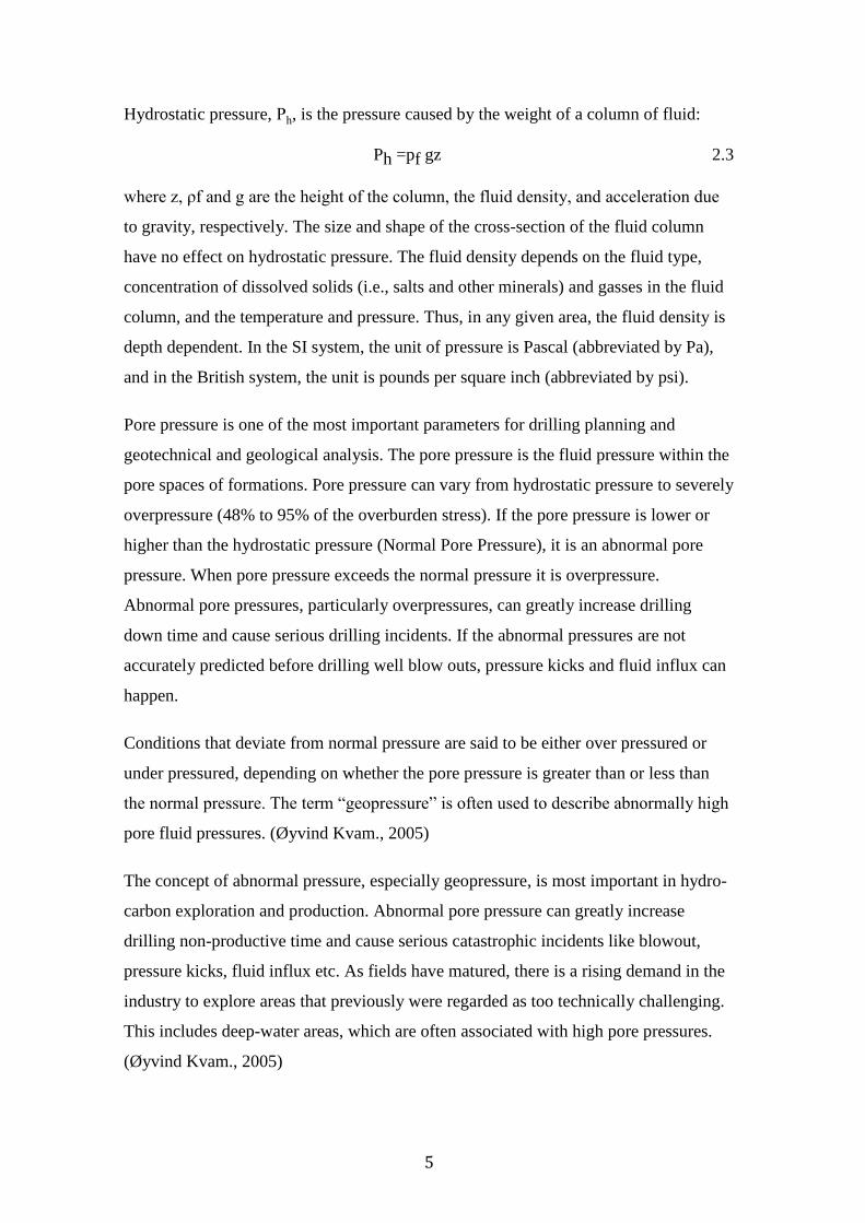
As illustrated by Figures 2.4 and 2.5, the wellbore pressure increases as circulation of

drilling fluid and transport of cuttings occur, thus BHPdyn > BHPstat. It is important to

consider both the static and the dynamic wellbore pressures during the planning and

drilling phase of a well. The static wellbore pressure must be sufficient to keep the

wellbore pressure above the formation-pore pressure, whereas the dynamic wellbore

pressure must stay below the formation-fracture pressure. This may pose problems in

narrow mud weight windows, and thus cause losses/influx to occur which eventually

may trigger the need for setting casing/liner earlier than planned.

14

Fig2.5 Static wellbore pressure to the right and dynamic wellbore pressure to the left

during conventional drilling.

2.3.2 Underbalanced Drilling

Underbalanced drilling is, as opposed to conventional drilling, successfully achieved

when the effective circulating borehole pressure is less than the formation-pore

pressure, thus (Golan, M.,2014):

BHP < Pf 2.11

This implies that an influx of formation fluid is intentionally invited into the wellbore.

In order to accurately control and regulate the wellbore underbalance, and thus the

amount of formation fluid influx, external back pressure is applied from the surface).

The static bottom hole pressure during UBD is then expressed as (Golan, M.,2014):

BHPstat = ρm · g · T V D + PBP,stat 2.12

where PBP,stat is the amount of back pressure applied during static conditions. When

the mud pumps are turned on and circulation initiated, the bottom-hole pressure is

expressed as (Golan, M.,2014):

BHPdyn = ECD · g · T V D + PBP,dyn 2.13

15

Where PBP,dyn is the amount of back pressure applied during dynamic conditions. As

illustrated by Figure 2.6 and, the amount of backpressure applied during static and

dynamic conditions may be regulated so that a more stable bottom-hole pressure is

obtained.

If a porous fluid containing formation is drilled through underbalanced, fluids will

enter the wellbore. This makes it more complicated to estimate the bottom-hole

pressure during both static and dynamic conditions especially if the formation fluid is

gas, which will displace and replace drilling fluid. This will cause the wellbore

pressure to decrease as gas normally has a lower density than drilling fluid. The

relatively low density of gas combined with fluid circulation, causes the gas to migrate

towards the surface. As gas rises and the hydrostatic fluid pressure decreases, the gas

will expand and cause even more drilling fluid to be displaced. From a conventional

point of view, the situation described above is considered as a kick, that is an

uncontrolled influx of formation fluid. However, during underbalanced drilling it is the

intention to invite drilling fluid into the wellbore. Through the invention of back

pressure, such a situation can effectively be controlled in a safe manner. If suddenly

the flow of formation fluids exceeds a wanted value, the back pressure can be

increased slightly, thus avoiding an uncontrollable situation (Golan, M.,2014)

Fig2.6 Static wellbore pressure to the right land dynamic wellbore pressure to the left

during underbalance drilling

16

Underbalanced drilling is normally more costly and time-consuming than conventional

drilling. Despite this, underbalanced drilling has evolved to become a relatively

common procedure. Mainly because an underbalanced well induces very little damage

to the formation, which is especially appreciated when drilling the reservoir section.

Oil/gas production is thus enhanced and the need for expensive well stimulation is

eliminated. In addition, masked or subtle hydrocarbon pay zones may be discovered

during underbalanced drilling (reveals itself by generating a kick) [(Golan, M.,2014);

(Olsen, E.J, 2012b)].

There are however some disadvantages associated with UBD, such as [(Olsen, E.J,

2012c);(www.egyptoil-gas.com)]:

• Increased overall production risk

• Wellbore instability.

• Well control issues.

• Increased drill string vibration and higher torque and drag.

• Problems with the MWD mud pulse signals.

• Problems related to flaring, storing or injection of the formation fluids transported to

surface during drilling

2.3.3 Managed Pressure Drilling

In 2004, the IADC defined MPD as: “An adaptive drilling process used to precisely

control the annular pressure profile throughout the wellbore (www.iadc.org).“ The

stated objectives are to: “Ascertain the downhole pressure environment limits and to

manage the annular hydraulic pressure profile accordingly (www.iadc.org).” The

IADC effectively differentiates MPD from UBD by stating the following: “It is the

intention of MPD to avoid continuous influx of formation fluids to the surface. Any

influx incidental to the operation will be safely contained using an appropriate process

(www.iadc.org).” In order to achieve this stated intention, MPD is performed with a

BHP at, or slightly above the pore pressure, thus:

BHP ≥ Pf 2.14

Problems related to lost circulation and wellbore kicks can to a great extent be

mitigated through MPD. If it is sensed that drilling fluid is being lost to the formation,

the back pressure can quickly be reduced to bring the wellbore pressure below the

17

formation-fracture pressure. The amount of drilling fluid actually lost and the damage

exerted on the formation is then very low due to the rapid response .The

same principle applies if a kick is detected. The back pressure is increased to bring the

wellbore pressure above the formation-pore pressure, thus quickly bringing the

situation under control (Haghshenas et al., 2008)

Fig2.7 Lost circulation to the left and kick to the right (www.drilling-mud.org)

During overbalanced drilling in porous/permeable formations, a filter cake is formed

along the borehole wall. This filter cake consists of cuttings and precipitated particles

from the drilling fluid. The pressure gradient in the filter cake varies from wellbore

pressure to pore pressure at the borehole wall. If a sufficient amount of the drill string

is embedded in the filter cake, movement/rotation of it becomes impossible. This

situation is referred to as a differentially stuck pipe, illustrated in Figure 2.7.

Differential sticking is the most frequent stuck pipe cause, and thus a great contributor

of non productive time (NPT). As the wellbore overbalance is kept very low during

MPD, the occurrence of differential sticking is greatly reduced with this drilling

technique (Kinn, A.A., 2013)

2.4 Pressure control during drilling

A fundamental requirement for a safe and responsible drilling operation is proper

control of the wellbore pressure. The wellbore pressure must be sufficiently high to

avoid a collapsed borehole situation and/or unwanted influx of formation fluids,

referred to as a kick. Meanwhile, the pressure in the wellbore must not exceed the

18

maximum pressure the formation is able to withstand. If this occur, fractures will be

formed along the borehole wall and drilling fluid will be lost to the formation, referred

to as lost circulation. The pressure conditions at which these incidents occur are

commonly presented in a plot known as the mud weight window (Fjaer. E. et al.,

2008).

Until the early 1900s, drilling after hydrocarbons were conducted without any form of

pressure control whatsoever. The hydrocarbons encountered during drilling would flow

uncontrolled to the surface and lead to a blowout. An unwanted influx of formation

fluid is, as mentioned above, referred to as a kick. However, if the ability to control

this influx is lost and hydrocarbons are flowing with an uncontrollable rate towards the

surface, the situation has developed to a much more serious situation, namely a

blowout. Such a situation may potentially inflict large economic consequences, and in

a worst case scenario involve loss of human lives. The aforementioned drilling strategy

in the early 20th century caused several blowouts to occur, such as the Spindletop

blowout on January 10, 1901. On that day, it was reported in the morning news that a

solid stream of petroleum roses out of the earth, 200 feet (61 meter) into the air. The

Spindletop well flowed uncontrolled for nine days before it was finally brought under

control, leaking up to 100 000 barrels (15 900 m3) per day. A picture taken of the

Spindletop blowout is presented in figure 2.8 (Langley, W.D and Dunsavage, P.M,

1970)

Fig2.8 Spindletop blowout in 1901 ((Langley, W.D and Dunsavage, P.M, 1970)

19

2.5 Uncertainty of measurement

2.5.1 Introduction

The term “uncertainty of measurement” was established to uniform the terminology.

“The uncertainty of measurement is a parameter, associated with the result of a

measurement, that characterizes the dispersion of the values that could reasonably be

attributed to the measurand.” .The measurand is the particular quantity to be measured.

The term “uncertainty of measurement” is sometimes used only as “uncertainty” but it

may have also another meaning. In metrology, the term “error” does not mean the

same thing as “uncertainty”. (Bell., S, 2001)

Uncertainty is a quantification of the doubt about the measurement result while error is

the difference between the measured value and the true value of the object being

measured. The importance of determining uncertainties should be obvious. No result

can be considered understandable without the associated uncertainty. Errors and

uncertainties come from very different sources which all have to be examined and

uncertainties estimated. (Bell., S, 2001)

In a measuring process, the sources may be such follows (Bell., S, 2001):

The measuring instruments (EDM instrument, reflector, thermometer and barometer.

The item being measured (calibration baseline)

The measurement process (measurement procedure)

Imported uncertainties (projection correction, instrument calibrations)

Operator skill (measurer)

The environment (atmospheric conditions),

Sampling issues (atmospheric conditions determined at a wrong place)

Accurate and reliable well bore pressure prediction is necessary for safe drilling

operations, especially now that oil and gas operators venture into more-challenging

environments. Drilling program are designed to stay within the operating window

between pore pressure and fracture pressure profile in the subsurface but in some cases

difficult challenges occur that make it difficult for the drilling company to drilled a

well within a good margin of operating window, thereby increasing the possibility of

taking a risk of kick, collapsing or fracturing. Therefore, it is very critical to have

precise control on wellbore pressure, failing result into a catastrophic incident.

20

A wide range of parameters is required for accurate study, many of which are subject

to uncertainties caused by measurement errors. Error also can be introduced into data

through the methods of interpretation used. Imperfect or lack of human knowledge of a

system is another source of input uncertainties. (Bell., S, 2001)

2.5.2 Uncertainty in measurement of sensor

This portion will be related to the uncertainty involved in accuracy and measurement

of the sensor itself which in turn could have a major impact on the uncertainty of the

wellbore pressure regime.

Sensor allow us to quantify the data and information at a given point .in space and

time. The data from a sensor represents an historic record of the subsurface property at

a. specific point and time of measurement. It is very important to consider exactly

what the sensor reading represents, i.e annular pressure within borehole represents the

cumulative effect of different forces impact on sensor reading.For example, in case of

circulating well, the pressure sensor will provide data comprising both of hydrostatic

fluid column and frictional effects caused by circulation of the fluids. So this

information can be. thought of as the superposition of a multitude of different pressure

events. occurring simultaneously, each with a potentially changing magnitude in time. .

It is important to know the different process that is going on in wellbore. .By knowing

this information we could attribute different value to different processes or components

thereby .generating baseline measurement. Once the baseline measurement is

established, .variation of the measured data needed to be calibrated to get the best

result.(Coley, J. C & Edwards, T.S 2013).

For data analysis, accuracy of sensor is required but unfortunately all sensors exhibit

some degree of inaccuracy and this can be reduced significantly by calibrating the

individual sensor across a range of anticipated operating condition. .By comparing the

measured values to the actual test values the behavior .of sensor can be accurately

characterized to adjust the sensor output (Coley, J. C & Edwards, T.S 2013)..

There is always an issue with sensor error and how could .it have impact on calculated

value of subsurface pressure. Fig 2.9 shows a depth-based path of annular. pressure

data for one of the section drilled. The sensor data is plotted against a calculated

21

hydrostatic pressure curve. From the figure, one of the sensors (designated 969)

consistently reports a pressure significantly higher than the other sensor in the well.

This offset appears to be constant and does not show any indication of drifting further

from the true value, which suggest some degree of constant offset error (Coley, J. C &

Edwards, T.S 2013)

22

Fig2.9 Plot of MD(ft) versus Annular Pressure (psi), the constant discrepancy in the value reported by X-Link969 (Coley, J. C & Edwards, T.S

2013)..

23

3. Methodology 3.1 Data

Data were gathered from different Wire Pipe Automation Project for wells drilled in

the USA. Drilling Automation System Provider is responsible for enabling drilling

automation job. Data measured by downhole sensors are transferred through network

drillstring. In several drilling automation jobs, there are multiple sensors that collect

data. Every 2.56 sec, each dataset is statistical summary of 2048 samples of pressure

measurement (figure 3). Generally, we have multiple tools located at BottomHole

Assembly (BHA) and along the drillstring. This data is sent in real time to the surface

system where it is decoded and then sent to the integration platform. The Integration

platform then supplied this data to application including data logging, and to the user.

24

Fig 3 How the drilling data is recorded in a real time. (Courtesy Drilling Company)

25

3.2 Methods

There are certain techniques that need to be employed to estimate pressure at the point

other than the measured one along the borehole. Each method has its own limitation

depends upon whether it is employed in static or circulated state and the geometry of

the well. We assume that at any point in the borehole we have the pressure P,

consisting of hydrostatic and frictional pressure components.

The general equation to measure Pressure at any point is given by

P = P1 + ∆𝑃ℎ𝑦𝑑 + ∆𝑃 𝑓𝑟𝑖 3.1

To manipulate whether hydrostatic pressure dominates friction pressure, there are

general practices that need to be considered (table 3).

Table 3

State of the

well

Geometry of the

well

Pressure State

Hydrostatic

Pressure

Friction Pressure

If the well is in

static state Vertical position Significant

Insignificant

If the well is in

static state Horizontal position Significant

Insignificant

If the well is in

circulation state Vertical position Significant

Significant

If the well is in

circulation state Horizontal position Significant

Significant

If the well is in

static condition Inclined position Significant

Insignificant

If the well is in

circulation

condition

Inclined position Significant Significant

Based on above-mentioned criteria, three methods are proposed which are:

3.2.1 Method A (Pressure estimates based on Measured Distance (MD))

26

3.2.2 Method B (Pressure estimated based on True Vertical Depth (TVD)).

3.2.3 Method C (Pressure estimated based on Decomposition)

3.2.1 Method A (Pressure estimates based on Measured Distance (MD))

Method A is based on linear relationship between the two pressure point along the

measured depth in the borehole. Let us consider a point I at any distance between the

two pressure point i.e P0 and P1. . The Measured Depth (MD) at point I is given as

MDI and with respect to pressure at point 0 or 1 is MD0 and MD1 respectively.

The Pressure at point I is calculated by following equation which is given by:

Pi= P0+( P1-P0) 𝑀𝐷𝐼−𝑀𝐷0

𝑀𝐷1−𝑀𝐷0 3.2

However, Method A has some limitation if we change the geometry of the well and

whether if the well is static and circulated .

3.2.2 Method B (Pressure estimated based on True Vertical Depth (TVD)).

The Method B relies on true vertical depth of any pressure point along the borehole

with respect to the surface. The True Vertical Depth (TVD) at point I is given as TVDI

and with respect to pressure at point 1 or 2 is TVD1 and TVD2 respectively.

Hydrostatic pressure increases with depth of the well. So in this case. hydrostatic

pressure will be maximum as compared to the friction pressure. Friction pressure will

only be greater as compared to the hydrostatic pressure, if there is high flow rate,

higher viscosity etc.

The pressure at point I is calculated by following equation

Pi= Po+ (P1-Po) +𝑇𝑉𝐷𝑖−𝑇𝑉𝐷2

𝑇𝑉𝐷1−𝑇𝑉𝐷2 3.3

3.2.3 Method C (Pressure estimated based on Decomposition)

This method works on the approach that Hydrostatic pressure will be based on True

Vertical Depth (TVD) and Friction pressure will be based on Measured Depth (MD).

During Drilling operation, pressure generated from one point to another along the

borehole called as pressure difference. These pressure difference are assumed to be

composed of two components i.e static pressure and friction pressure.

27

Method C works on the principle by which if measured pressure and condition of the

well are known, then the two components of the pressure difference could be

separated. It is based on linear interpolation of two points using TVD on static

component and measurement depth on frictional components.

For this method, we have to check of the well is static or not

If well is static, then compute pressures using TVD-based linear interpolation of static

pressures given as

Piestimated = P1 + (P2-P1) x (TVDi- TVD1)/(TVD2- TVD1) 3.4

In case, if well isn’t static then hydrostatic component of pressure using TVD-based

linear interpolation of static pressures given as

Pihyd = P1 Pstatic + (P2 Pstatic -P1 Pstatic ) x (TVDi-TVD1)/(TVD2- TVD1) 3.5

And then compute frictional component of pressure using MD-based linear

interpolation of computed frictional pressures given as

∆Pifric = ∆P1fric + (∆P2fric -∆P1fric ) x (MDi-MD1)/(MD2- MD1) 3.6

Finally, estimated pressure is then combination of hydrostatic and frictional component

given as

Pestimated = Phydrostatic + ∆Pfriction 3.7

3.3 Data Processing and Data Analyzing

The raw data recorded on rig at one second intervals is collected in the form of Well A

drilling dataset version 0.csv which is reduced to time interval with minimum of three

down hole sensor measurement along the drill string. The raw data then need to be

processed for quality checking , data cleanup and elimination of irrelevant data (See

Appendix). There are several steps and procedures that need to be done once drilling

data is acquired. For this specific dataset, these steps are;

Initial data:

Well A drilling data entire well.csv- all drilling data for well

28

Well A drilling data VER 0.csv – dataset reduced to timer interval with

minimum of 3 downhole annular pressure measurements

Well A directional survey.csv – Directional survey, including MD vs TVD data

for well

This is the planned procedure for processing and analyzing the data for this well. Note:

The value -999.25 is used to denote invalid data.

Following are the four steps that need to be carried out to estimate the predicted

pressure from the raw data which are:

Step 1 – Generate Well A drilling data VER 1.csv, as follows:

Start with Well A drilling data VER 0.csv.

Mark all Mud Weight In and Out values as invalid.

Manually add some surface-measured Mud Weight In and Out values.

Step 2 - Generate Well A drilling data VER 2.csv, as follows (using App1):

Start with Well A drilling data VER 1.csv.

Compute Measured Depth for each sensor, by subtracting Bit-to-sensor

distance from Bit Position, and add to data file.

Compute TVD for each sensor, by linear interpolation using MD vs TVD data,

and add to data file.

o TVDi = TVD0 + (TVD1-TVD0)x(MDi-MD0)/(MD1-MD0)

Compute SMW-estimated static pressures at each sensor (SMW = Surface Mud

Weight In and Out) for each sensor, and add to data file. Equation for this is:

o P = 0.052 * MW * TVD

o MW = mud weight, ppg

o TVD = true vertical depth, ft

o P = pressure, psi

Visually compare SMW-estimated pressures with measured data, to verify that

measured data and Bit-to-sensor data is reasonable.

Step 3 - Generate Well A drilling data VER 3.csv, as follows (using App2):

Start with Well A drilling data VER 2.csv.

Identify invalid pressure measurements and mark as invalid.

29

o Pressure data is output every 2.56 seconds, so after 3 seconds of no

change a pressure value is considered to be invalid.

o Visually observe data. Remove any obvious outliers that appear to be

not from specific sensor.

Add static pressure data at all measurement points. Do this by:

o Identify static states with valid data and store measured pressure as

static pressure.

o Mark all other static pressure values as invalid.

Generate all possible (12, from 4 x 3) pressure predictions for intermediate

points using each of the 3 methods as already discussed earlier and add to

dataset.

o Method A – “MD-Based”

Compute pressures based on linear interpolation of measured

depth, using current measured pressures. Equation is:

Pi = P1 + (P2-P1)x(MDi-MD1)/(MD2-MD1)

o P = pressure, psi

o MD = measured depth, ft

o All depths are in feet.

o Point i denotes the measured depth at which a

pressure prediction is desired.

o Points 1 and 2 specify the sensors which are on

either side of point i.

o Method B – “TVD-Based”

Compute pressures based on linear interpolation of measured

depth, using current measured pressures. Equation is:

Pi = P1 + (P2-P1) x (TVDi-TVD1)/(TVD2-TVD1)

o P = pressure, psi

o TVD = measured depth, ft

o All depths are in feet.

o Point I denotes the true vertical depth at which a

pressure prediction is desired.

o Points 1 and 2 specify the sensors which are on

either side of point i.

30

o Method C- “Decomposition”

Determine if well is static or not.

If well is static:

o Update static pressures (i.e. record)

o Compute pressures using TVD-based linear

interpolation of static pressures.

Piestimated = P1 + (P2-P1) x (TVDi- TVD1)/(TVD2-

TVD1)

Else if well is not static:

o Compute hydrostatic component of pressure using

TVD-based linear interpolation of static pressures

(i.e. the latest ones recorded).

Pi hyd = P1 P static + (P2 P static -P1 P static ) x

(TVDi-TVD1)/(TVD2- TVD1)

o Compute frictional component of pressure using

MD-based linear interpolation of computed

frictional pressures.

Compute frictional components at points 1

and 2:

∆Pfric = P – P static .

Interpolate frictional component at point i

∆Pi fric = ∆P1fric + (∆P2fric -∆P1fric ) x

(MDi-MD1)/(MD2- MD1)

o Compute estimated pressures as sum of hydrostatic

and frictional pressures.

Pestimated = Phydrostatic + ∆Pfriction

Step 4 – Assess estimation of pressure predictions

Generate predicted pressure from three methods.

Analyze predicted pressure and draw conclusions as to effectiveness of

pressure prediction methods.

31

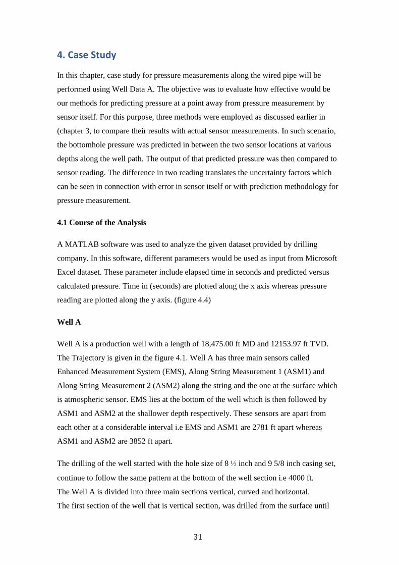
4. Case Study In this chapter, case study for pressure measurements along the wired pipe will be

performed using Well Data A. The objective was to evaluate how effective would be

our methods for predicting pressure at a point away from pressure measurement by

sensor itself. For this purpose, three methods were employed as discussed earlier in

(chapter 3, to compare their results with actual sensor measurements. In such scenario,

the bottomhole pressure was predicted in between the two sensor locations at various

depths along the well path. The output of that predicted pressure was then compared to

sensor reading. The difference in two reading translates the uncertainty factors which

can be seen in connection with error in sensor itself or with prediction methodology for

pressure measurement.

4.1 Course of the Analysis

A MATLAB software was used to analyze the given dataset provided by drilling

company. In this software, different parameters would be used as input from Microsoft

Excel dataset. These parameter include elapsed time in seconds and predicted versus

calculated pressure. Time in (seconds) are plotted along the x axis whereas pressure

reading are plotted along the y axis. (figure 4.4)

Well A

Well A is a production well with a length of 18,475.00 ft MD and 12153.97 ft TVD.

The Trajectory is given in the figure 4.1. Well A has three main sensors called

Enhanced Measurement System (EMS), Along String Measurement 1 (ASM1) and

Along String Measurement 2 (ASM2) along the string and the one at the surface which

is atmospheric sensor. EMS lies at the bottom of the well which is then followed by

ASM1 and ASM2 at the shallower depth respectively. These sensors are apart from

each other at a considerable interval i.e EMS and ASM1 are 2781 ft apart whereas

ASM1 and ASM2 are 3852 ft apart.

The drilling of the well started with the hole size of 8 ½ inch and 9 5/8 inch casing set,

continue to follow the same pattern at the bottom of the well section i.e 4000 ft.

The Well A is divided into three main sections vertical, curved and horizontal.

The first section of the well that is vertical section, was drilled from the surface until

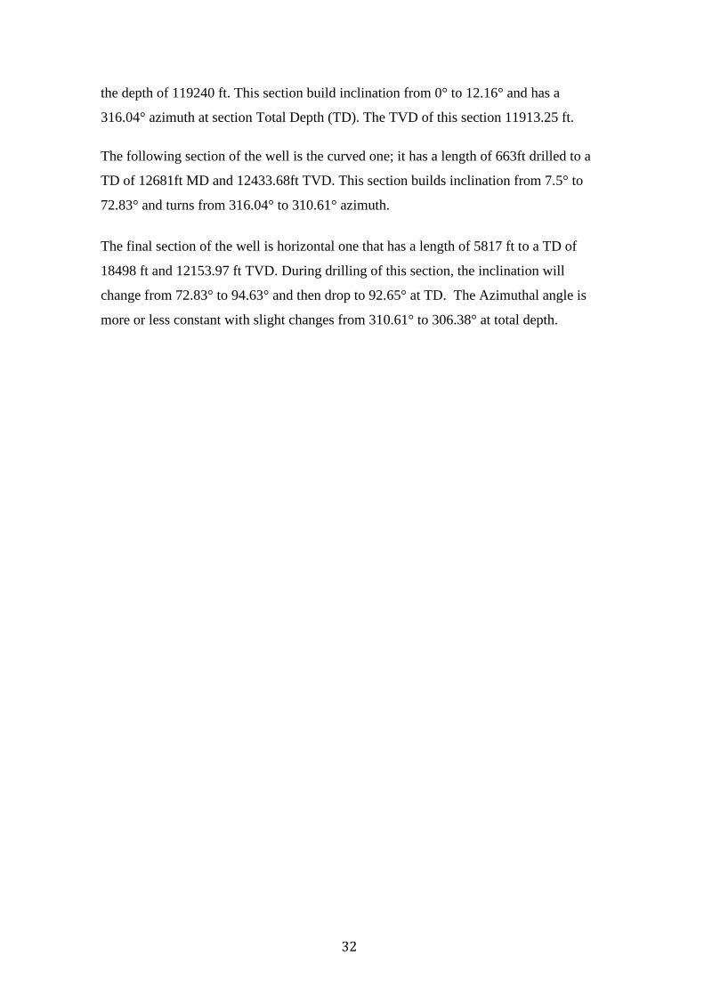
32

the depth of 119240 ft. This section build inclination from 0° to 12.16° and has a

316.04° azimuth at section Total Depth (TD). The TVD of this section 11913.25 ft.

The following section of the well is the curved one; it has a length of 663ft drilled to a

TD of 12681ft MD and 12433.68ft TVD. This section builds inclination from 7.5° to

72.83° and turns from 316.04° to 310.61° azimuth.

The final section of the well is horizontal one that has a length of 5817 ft to a TD of

18498 ft and 12153.97 ft TVD. During drilling of this section, the inclination will

change from 72.83° to 94.63° and then drop to 92.65° at TD. The Azimuthal angle is

more or less constant with slight changes from 310.61° to 306.38° at total depth.

33

Fig4.1 Three dimensional directional survey for Well A with three different sensors at different location

34

Figure 4.2 displays the temperature profile for Well A. The x-axis is represented by the

Temperature in ºC whereas y-axis is represented by True Vertical Depth (TVD) in ft.

As seen from the figure, the temperature gradually increases with depth during drilling

operation and it continues to increase to a depth of 11600 TVD ft where we notice

decrease in temperature resulting from change in pipe connection for which drilling

operation halts for some time and also possibly caused by extended circulation of the

fluid to cool the well. Connection of the drilling pipe normally occurs after 93 ft during

the course which results into the decrease in temperature. As drilling operation

resumes, we have notice the same trend i.e increase in temperature throughout the

section except at the bottom of section where we have seen abrupt increase in the

temperature profile suggesting that the wellbore fluid in the lateral direction of the well

is harder to cool, resulting into the sharp increase in temperature.

35

Fig4.2 Temperature profile for Well A.

36

To perform the analysis, a set of basic criteria have been set. These parameters are

according to those measured while drilling and given in the daily drilling reports and

also including data that has been processed manually.

4.2 Prediction of Pressure

Prediction of pressure will be carried out based on three sensors along string. A total of

12 pressure prediction will be made to estimate pressure in between two sensor along

the string. These predictions will be established by using three methods that have

already been discussed in chapter 3.

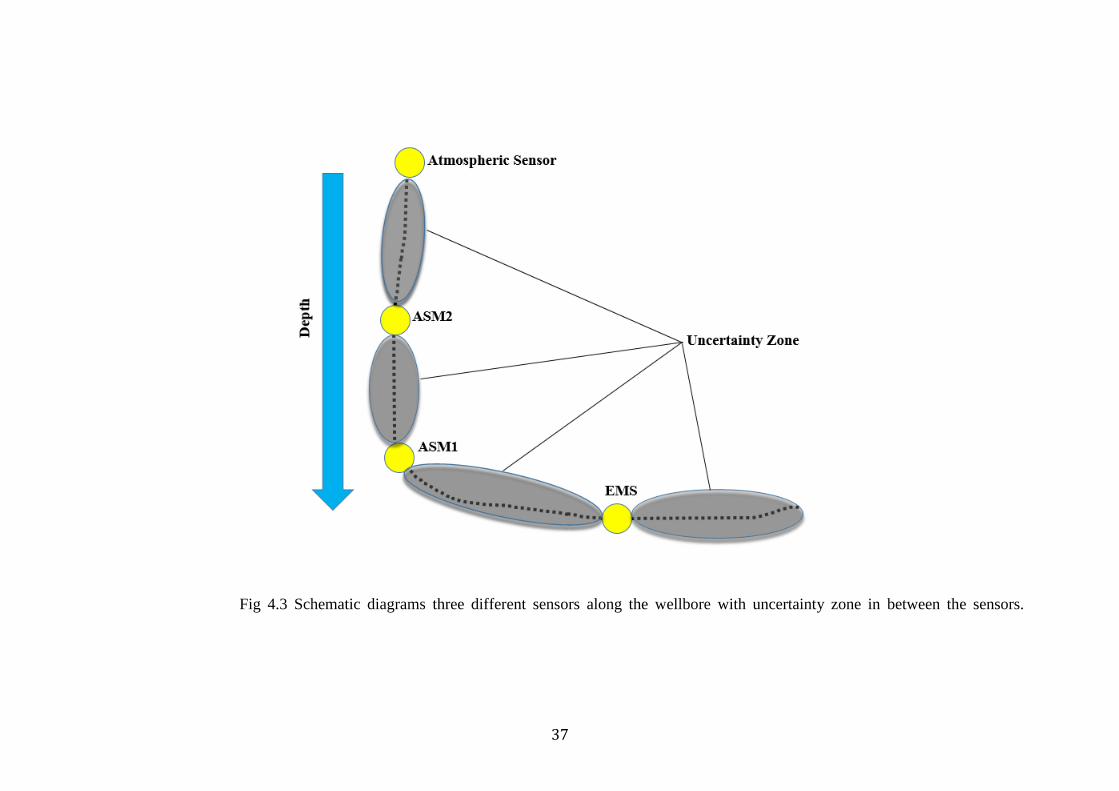
Pressure at a certain sensor location is known and to predict pressure measurement in

between sensors, there lie a lot of uncertainties (figure 4.3). Our objective is to

accurately estimate these pressures, therefore, we employ a simple concept that runs on

a principle that predicted pressure at an area of interest is equal to the either side of the

known (measured) pressure at sensor location. Through this technique, not only we can

able to predict pressure in between the points but also to check the effectiveness of

predicted pressure against the measured one

37

Fig 4.3 Schematic diagrams three different sensors along the wellbore with uncertainty zone in between the sensors.

38

In figure 4.4, pressures are recorded by three different sensors below the casing shoe

are displayed. The x-axis represent the time in seconds during the drilling operation

whereas y-axis represents the pressure recorded by sensors in psi. The blue lines

displays the pressure recorded by deeper sensor i.e EMS and is denoted by P0 whereas

red and yellow lines display the pressure recorded by shallower sensors called ASM1

and ASM2 respectively and are denoted by P1 and P2 respectively. P3 sensor which is

at surface is an atmospheric sensor and is constant(i.e. atmospheric pressure).

Trend in pressure measurement shows the linear relationship. With the time, pressure

continues to increase throughout the section. The dip along the pressure readings

results from change in connection of pipe during drilling operations. It is noted that in

the beginning of the section, especially in case of ASM1and ASM2 sensor data, some

of the data are missing due to the invalid dataset.

39

Fig 4.4 Pressure reading from three different sensors

40

In order to analyze the effectiveness of our methods (as illustrated in chapter 3) ,the

predicted pressure along the wellbore was compared to the pressure measurement by

sensor itself. This was performed by each seconds along the wellbore section. For each

point of sensor along the section, pressure was measured and recorded in surface in

real time. It is noted that the pressure can only be recorded where the sensor is

currently located in real time. During the drilling operation, pressure was recorded

where the sensor was located. Therefore, we have to rely on prediction method to

estimate the pressure in between the sensor point.

4.2.1 Prediction of Sensor 1 (Based on Sensor 0 and Sensor 2)

Figure 4.5 shows the comparison of predicted pressure versus measured one. The

pressure was predicted in between the two sensors point i.e at Sensor 0 (EMS) and

ASM2 (Sensor2). Three methods were employed to compare predicted pressure versus

measured one by sensor 1(ASM1). Based on the figure, it seems that in the beginning

of the section three predicted pressure are more or less superimposed on measured one

but then later in the section around 1500000 predicted pressure (P102-A) proceeded

below the measured one by a difference of almost -1000 psi. The two other predicted

pressure (P102-B & P102-C) are superimposed on each other and proceeded above the

measured one by a difference of almost +1000 psi.

41

Fig 4.5 Comparison of predicted pressure versus measured one for sensor 1 (Based on Sensor 0 and Sensor 2) with the geometry of the well in

small window

42

4.2.2 Prediction of Sensor 1 (Based on Sensor 0 and Sensor 3)

Figure 4.6 displays the comparison of predicted pressure (between Sensor 0 and Sensor

3) versus measured one Sensor 1. In the beginning of the figure, all of the three

predicted pressure are more or less overlapping on each other but then later in the

section at about1500000 seconds predicted pressure for sensor1 tend to drift away from

the measured pressure. Predicted pressure (P103A) drifted away from the measured

one by difference of -1000psi whereas predicted pressure (P103B and P103C) by a

difference of +1000psi respectively

43

Fig 4.6 Comparison of predicted pressure versus measured one for sensor 1 (Based on Sensor 0 and Sensor 3) with the geometry of the well in

small window

44

4.2.3 Prediction of Sensor 2 (Based on Sensor 0 and Sensor 3)

Figure 4.7 displays the comparison of predicted pressure (in between the Sensor 0 and

Sensor 3) versus measured one (Sensor 2). Based on the figure, predicted pressure has

drifted away from the measured one throughout the section. In the beginning, the

predicted pressure drifted away from the measured one by a difference of 200 until the

point where the section reaches 1500000 seconds. After that three of our predicted

pressure sign off in different direction i.e the predicted pressure (P203 A) are more or

less superimposed on measured one through the section of 1500000 to 17500000 and

then drifted below by a difference of 500 psi at the end of the section, whereas

predicted pressure (P203B and P203C) never superimposed on the measured pressure

and continue to drifted above from the measured one by a difference of 800 psi.

45

Fig 4.7 Comparison of predicted pressure versus measured one for sensor 2 (Based on Sensor 0 and Sensor 3) with the geometry of the well in

small window

46

4.2.4 Prediction of Sensor 2 (Based on Sensor 1 and Sensor 3)

Figure 4.8 displays comparison of predicted pressure (in between Sensor 1 and Sensor

3) versus measure pressure (Sensor 2). All of the three predicted pressure

(P213A,P213B and P213C) are superimposed on each other and drifted away from the

measured pressured by a difference of more or less 100 psi throughout the section but

then later in the section around 2300000 seconds, one of the predicted pressure (P213

A) trending towards the measured pressure (Sensor 2).

47

Fig4.8 Comparison of predicted pressure versus measured one for sensor 2 (Based on Sensor 1 and Sensor 3 with the geometry of the well in

small window

48

5. Discussion This chapter presents discussions based on the findings from the analyses. Discussions

regarding the credibility of the analysis including simulator biases and other effects

that may produce misleading results will be presented.

5.1 Deviation with respect to the geometry of the well

The well geometry plays a part in how much of the well is affected by applying

backpressure at the surface. If the well is static and completely horizontal at some

section, the pressure in this section would be constant as the TVD is the same.

Consequently, addition of backpressure at surface would result in the same pressure

increase in each part of the horizontal section. However, if the well is vertical, the

pressure will be different as the TVD is not constant along the wellpath. This is only

true when the well is static, like during connections. If there is circulation, the friction

loss will depend primarily on the well length and secondary on the geometry of the

well.

5.1.1 Pressure Prediction

This thesis features some of the information from International Research Institute of

Stavanger (IRIS). This information relates to the estimation of pressure at any point

along the well. However, this thesis does not employ modeling technique to estimate

pressure but instead used simple interpolation methodology to estimate pressure in

between the sensor points along the well. (Erick, C and Lande. H.P., 2013)

Well geometry and positioning of sensors along the drill pipe plays an important role

in predicting pressure in between the sensor points. The more constant the geometry of

the well would be, the more likely the prediction of the pressure would be

superimposed upon the measured one. As the sensor moves along the drill pipe during

the drilling operation, some of the sensors move past the vertical section of the well

and ended up in either curved part or horizontal section of the well. This could also

influence the prediction of the pressure based on whether sensor is located in vertical,

curved or horizontal part of the well.

5.1.2 Error in Pressure Prediction

Different methods have been applied to check the effectiveness of our prediction with

respect to the measured pressure. Every method has some limitation and weakness

49

depending upon geometry of the well and condition of the well i.e whether well is in

static or flowing condition.

We assume that hydrostatic component is the dominant contributor to the pressure i.e

93% EMS sensor when the well is in circulated mode and 100 % in static well. This

would have impact on estimating pressure when interpolating between the two points

along the wellbore.(in between the EMS sensor and sensor at the surface)

We assume that if the well is static, in such case hydrostatic component would be

dominant and therefore, method B predicts pressure more precisely than method A and

if the well is flowing, in such case there will be a frictional component as well as

horizontal component. However if the well is vertical positioned, then method A and

method B would be identical as both measured depth and true vertical depth are same,

in that case method B would be more applicable in predicting pressure accurately than

method A.

The hydrostatic component of pressure is mis-represented by Method A, as Method A

effectively assumes the hydrostatic component is a function of measure depth, when in

reality it is linearly related to true vertical depth. Using the wrong depths produces a

wrong linear estimate, which is usually low due to the relationship between measured

depth and true vertical depth (true vertical depth is always equal to or less than

measured depth).

For Method C, there are two component including hydrostatic component as a function

of true vertical depth and frictional component as a function of measured depth.

The error that we have seen in our prediction for method C especially at the end of the

section could be caused by the assumption that density would be the same during the

interval of static well. It is possible density would change during that time. For

example, when circulation and rotation stop, cuttings could fall out and settle on the

wellbore wall. This could produce the static density. When circulation and rotation

start, these cuttings could be re-suspended in the mud and its density would therefore

increase (without the knowledge of the method). This would introduce some error,

biased in one direction. Another possibility is the density increases as cuttings are

drilled and added to the mud, although if the annulus is fully saturated with same

concentration of cuttings from bit to surface, then it is in steady state (i.e. cuttings

drilled at same rate as cuttings removed).

50

The other causes of the error could be the measurement by sensor itself. EMS tool

started reading pressure high as it went further out in the lateral, with the high

temperatures being a big factor. The temperatures seen by the tool approached its

limits, and the tool later (i.e. after our data) failed. If P0 measured pressure at EMS

sensor is thus reading high, it would result in higher pressure estimates whenever it is

included.

5.2 Hypothesis

This subchapter present finding from the various papers/publications and is not directly

related to my thesis due to the lack of the data. However, It is important to mention

these facts and finding to better understand the scenario of the thesis project. The

whole idea of presenting these facts and finding is to correlate it with my findings to

better explain the uncertainties phenomenon both with the measurement of the sensor

itself and the factor that influence these uncertainties such as variation in mud density,

geothermal properties of formation rocks, flow of cutting along the well.

Uncertainty in the pressure could also be governed by change in mud density. The

effect of density uncertainty increases with length and depth of the well, both within

the same well and between different wells. This is reasonable to assume since the

hydrostatic well pressure is directly linked to the mud density. Increasing mud weight

also increases the casing shoe pressure. This increase is only affected by the setting

depth of the shoe and not the length of the section. This is also reasonable to assume

given that the hydrostatic pressure at a certain depth is only affected by the true

vertical depth of the overlaying fluid column. When density changes occur in a

downhole environment as a result of pressure, temperature, influxes and cuttings

transport, other parameters such as rheology is likely to change as well. This will

influence the downhole hydraulics and possibly give additional changes. . (Erick, C

and Lande. H.P., 2013)

Pressure variation in the measurement could also be affected by variation in

geothermal properties of formation rocks. Generally, increase in thermal conductivity

of the formation rocks increases the pressure and vice versa. However at more shallow

depth the uncertainty in thermal conductivity is strongly dominating. The resulting

pressure variations might be effected by both well depth and length of the openhole

51

section. . (Erick, C and Lande. H.P., 2013)

The relationship between heat transfer in the formation and the wellbore pressure is the

mud temperature. If more heat is transferred from the formation, the mud temperature

will increase and this will affect rheological properties and most importantly, the

density. (Erick, C and Lande. H.P., 2013)

5.3 Mud Window The mud weight window, occasionally referred to as the drilling operating window or

the drilling window, defines the maximum and minimum well pressure that is

acceptable during drilling. On the low side, the well pressure is bound by the

formation-pore pressure, Pf , or the collapse pressure of the formation . Whereas on the

high side, the well pressure is bound by the formation-fracture pressure, Pfra

Prior to drilling, a mud weight window is constructed based on estimations of the

underground stress and pressure environment. These estimations are then further used

to plan an optimal well design.

We assumed the pore pressure gradient across the South Texas where the well is

located as 0.465 psi/ft.

When pressures are related to mud density, it is customary to convert the pressure

value at a specific depth to a density value which is Equivalent Mudweight (EMW),

we have a formula

EMW= 0.465/0.052 = 9ppg (pound per gallon) 5.1

General Fracture pressure gradient of an area is 12.8ppg to 14 ppg. We assumed these

values based on the general trend of the well that has been drilled in these area (South

Texas, USA) (fig 5).

52

Fig5 Estimated mudweight window for Well A

Safety Margin

Pore Pressure

Fracture Pressure

53

6. Conclusion

This thesis has provided a new base that how uncertainties in the pressure regime

in the subsurface could be measured.

Three different methods were used to generate 12 predicted pressure in between

the sensors.

The geometry of the well plays an important role in contributing errors to

predicting pressure against the measured one.

The more vertical the path of the well would be, the more likely the predicted

pressure matches the measured one. As soon as well trend changes to curved or

horizontal path, predicted pressure would be way off from the measured one.

Each method has limitation and advantages in its own way depending upon the

geometry and condition of the well.

Among of all three methods, Method C rated the best one followed by Method B

and then Method A.

Uncertainties in mud density can generate significant pressure variations both at

the bottomhole depth and at another critical depth, a distance far away from the

downhole measurements

Uncertainties in formation geothermal properties such as an increase in either the

specific heat capacity or thermal conductivity will increase the wellbore pressure

and vice versa

Mud window were generated based on general geology of the SW Texas which are

then used to plan a optimal well design

54

7. Future Work The work presented in this thesis is a different approach to the effect on estimation of

pressure measurement in between the two points along the well bore. The effects that

influence the pressure estimation include mud-density variation, geothermal properties of

the formation rocks, reliability of the sensor itself etc. Future work on this topic would

include analysis of more cases studies i.e, for different well geometries, formation

properties and detailed analysis of cutting transport along the well. More simulations could

also be run in real time data for different configurations of pressure sensor types to isolate

the individual effect.

Future work could also be to have different well planning data so one could check the

viability of the proposed methodology presented in this thesis to estimate pressure

measurement. Once that has been established, such methodology should be employed for

the future projects to ensure safe and effective drilling operation.

55

8.Appendix Second

(sec)

Bit

position

(m)

Hole –

Depth

(m)

MD_0

(m)

MD_1

(m)

MD_2

(m)

TVD_0

(m)

TVD_1

(m)

TVD_2

(m)

P_0

(psi)

P_1

(psi)

P_2

(psi)

P1

0&2A

(psi)

P1

0&3A

(psi)

P2

1&3A

(psi)

P2

0&3A

(psi)

P1

0&2B

(psi)

P1

0&3B

(psi)

P2

1&3B

(psi)

P2

0&3B

(psi)

P1

0&2C

(psi)

P1

0&3C

(psi)

P2

1&3C

(psi)

P2

0&3C

(psi)

0 10141.2 10143.6 10064.24 7283.24 3496.24 10062.8 7282.3 3495.8 6677.8 4782.3 2188.7 4777.1 4832.6 2295.7 2319.8 4777.1 4832.6 2295.7 2319.9 -999.2 -999.2 -999.2 -999.2

1 10141.2 10143.6 10064.24 7283.24 3496.24 10062.8 7282.3 3495.8 6685.9 4782.3 2188.7 4781.7 4838.4 2295.7 2322.6 4781.8 4838.5 2295.7 2322.7 -999.2 -999.2 -999.2 -999.2

2 10141.2 10143.6 10064.24 7283.24 3496.24 10062.8 7282.3 3495.8 6685.9 4782.3 2197.0 4785.2 4838.47 2295.7 2322.6 4785.3 4838.5 2295.7 2322.7 -999.2 -999.2 -999.2 -999.2

3 10141.2 10143.6 10064.24 7283.24 3496.24 10062.8 7282.3 3495.8 6677.8 -999.2 2197.0 -999.2 -999.2 -999.2 2319.8 -999.2 -999.2 -999.2 2319.9 -999.2 -999.2 -999.2 -999.2

4 10141.2 10143.6 10064.24 7283.24 3496.24 10062.8 7282.3 3495.8 6677.8 -999.2 2188.7 -999.2 -999.2 -999.2 2319.8 -999.2 -999.2 -999.2 2319.9 -999.2 -999.2 -999.2 -999.2

5 10141.2 10143.6 10064.24 7283.24 3496.24 10062.8 7282.3 3495.8 6677.8 -999.2 2188.7 -999.2 -999.2 -999.2 2319.8 -999.2 -999.2 -999.2 2319.9 -999.2 -999.2 -999.2 -999.2

6 10141.2 10143.6 10064.24 7283.24 3496.24 10062.8 7282.3 3495.8 6677.8 4790.5 2197.0 4785.2 4838.4 2299.6 2322.6 4785.3 4838.5 2299.7 2322.7 -999.2 -999.2 -999.2 -999.2

7 10141.2 10143.6 10064.24 7283.24 3496.24 10062.8 7282.3 3495.8 6685.9 4790.5 2197.0 4785.2 4838.4 2299.6 2322.6 4785.3 4838.5 2299.7 2322.7 -999.2 -999.2 -999.2 -999.2

8 10141.2 10143.6 10064.24 7283.24 3496.24 10062.8 7282.3 3495.8 6685.9 4782.3 2197.0 4780.6 4832.6 2295.7 2319.8 4780.6 4832.6 2295.7 2319.9 -999.2 -999.2 -999.2 -999.2

9 10141.2 10143.6 10064.24 7283.24 3496.24 10062.8 7282.3 3495.8 6677.8 4782.3 2197.0 -999.2 4832.6 -999.2 -999.2 -999.2 4832.6 -999.2 -999.2 -999.2 -999.2 -999.2 -999.2

56

9. References “A new technology for reducing the density of drilling fluid”, [Online],

Downloaded from: http://www.egyptoil-gas.com/admin/industry/

Technology%20&%20Solutions%20Issue%207%20July%202007.pdf,

Bell, S. 2001 .A beginner guide for uncertainty of measurement. Measurement

Good practice guide number 11 (Issue 2) © Crown Copyright 1999.

Reproduced by permission of the Controller of HMSO. ISSN 1368-6550

Breckels, I.M. and van Eekelen H.A.M., “Relationship Between Horizontal

Stress and Depth in Sedimentary Basins”, this paper forms part Journal of

Petroleum Technology, Volume 34, Number 9, pages 2191-2199., September

1982. http://dx.doi.org/10.2118/10336-PA

(Borge 2000) Borge, H.:. Fault controlled pressure modelling in sedimentary

basins, Norwegian University of Science and Technology.

Bourgoyne A.T. Jr, et al.: “Applied Drilling Engineering,” SPE, Richardson,

TX, 1991, pp. 246 – 252.

Coley.J Christopher and Edwards, T.Stephen 2013. The use of along string

annular pressure measurements to monitor solid transport and hole cleaning.

SPE/IADC 163567 Drilling conference and exhibition.

Erick, C and Lande. H.P: “ Factor influencing the estimation of downhole

pressure far away from the measurement point during drilling operation” IRIS,

Stavanger, Norway, 2013.

Dutta, N. C2002, Geopressure prediction using seismic data: Current status and

road ahead: Geophysics, 67, 2012- 2041.

Fjær, E., Holt, R., Horsrud, P., Raaen, A. M., and Risnes, R., 1989, Petroleum

related rock mechanics: Elsevier.

Fjær, E., Holt, R.M., Horsrud, P. et.al 2008, “Petroleum Related Rock Me-

chanics”, second edition, Development in Petroleum Science, Elsevier

Golan, M., “IADC RIGPASS, Underbalanced Drilling Orientation”, Professor

at NTNU.

Gyllenhammar, Carl Fredrik (2003) A critical review of currently available

pore pressure methods and their input parameters: glaciations and compaction

57

of north sea sediments., Durham theses, Durham University. Available at

Durham E-Theses Online: http://etheses.dur.ac.uk/4090/

Haghshenas, A., Paknejad, A. S., Rehm, B. et.al 2008, “‘The Why and Basic

Principles of Managed Well-Bore Pressure”, Chapter one, Gulf Publishing

Company.

“IADC, Drilling Lexicon”, [Online], Downloaded from: http://

www.iadclexicon.org/equivalent-circulating-density-ecd/ (accessed

11.05.2014)

International Association of Drilling Contractors “Managed Pres- sure Drilling”

[online], Downloaded from: http://www.iadc.org/ ubo-mpd-

committee/subcommittees/

Kinn, A. A., “Comparison of Methods Enabling MPD from Floaters”, Special-

ization Project in the Unit TPG4520-Drilling Engineering at NTNU, autumn

2013.

Kvam.Øyvind., 2005. Pore pressure estimation from single and repeated

seismic data sets.A dissertation for the partial fulfillment of requirement for the

degree Doktor Ingeniør at the Department of Petroleum Engineering and

Applied Geophysics, Norwegian University of Science and Technology

Langley, W. D. and Dunsavage, P. M., “Pollution Control in the Oil Industry -

From Spindletop to Santa Barbara”, SPE-3096-MS, this paper was prepared for

the 45th Annual Fall Meeting of the Society of Petroleum Engineers of AIME,

Houston, Texas, U.S.A., 4-7 October 1970. http://dx.doi.org/10. 2118/3096-MS

Malinverno, A., Sayers, C.M., Woodward, M.J. and Bartman, R.C., 2004,

Integrating diverse measurements to predict pore pressure with uncertainties

while drilling: Paper SPE 90001, Society of Petroleum Engineers Annual

Technical Conference and Exhibition.

Olsen, E. J., “Managed Pressure Drilling (MPD), Subsea, History in Brief,

Drilling Technology”, Lecture presented in the unit “TPG4215,

Høyavviksboring” at NTNU, 12 October 2012a.

Olsen, E. J., “Underbalanced Operations, IADC Riggpass”, Lecture presented

in the unit “TPG4215, Høyavviksboring” at NTNU, 06 October 2012b.

Olsen, E. J., “UBO Theory” Lecture presented in the unit “TPG4215,

58

Høyavviksboring” at NTNU, 06 October 2012c.

[Online], Downloaded from: http://www.drilling-mud.org/,

Terzaghi, K., Peck, R.B., Mesri, G., 1996. Soil Mechanics in Engineering

Practice, 3rd Edition. John Wiley & Sons.

Zhang.J. The pore pressure prediction from well logs:Methods, modifications,

and new approaches, Shell Exploration and Production company, Houston,

Texas, USA., June 2011.