Embed Size (px)
Citation preview

CFD Modelling of Combined Blast and Contact Cooling for Whole Fish
Ma
ste
r T
he
sis
Valur Oddgeir BjarnasonMay 2012

CFD Modelling of Combined Blast andContact Cooling for Whole Fish
Master Thesis
By
Valur Oddgeir Bjarnason s100980May 16th 2012
Section for Fluid MechanicsDepartment of Mechanical Engineering
Technical University of Denmark
SupervisorsDr. Jens Honore Walther, Associate Professor, DTU, Denmark
Dr. Björn Margeirsson, Research Group Leader, Matis, IcelandSigurjón Arason M.Sc., Chief Engineer, Matis, Iceland

Preface
This thesis consists of four main chapters: Introduction, Materials and methods, Resultsand Discussion. The Introduction presents the CBC-cooling method and how it effectsfish quality and storage life. The Materials and methods chapter presents the experimentalsetup and which methods were applied to solve the CFD model. In the Results chapter theexperimental results are presented and compared with the simulated results. Finally theDiscussion chapter contains a review of the obtained results.
Combined blast and contact (CBC) cooling is a cooling method developed by thecompany Skaginn ltd (Akranes, Iceland) in cooperation with Marel (Garðabær, Iceland).The method is based on moving the product through a freezer tunnel where it is laid on analuminum belt while cold air is blasted on its surface. The name of the cooler has beenchanged to SuperChiller but is referred to as CBC-cooler in this thesis.
The experimental results presented in this work are a part of the research and devel-opment project Super-Chilled Round Fish - Pre Rigor, which was funded by AVS R&DFund of Ministry of Fisheries in Iceland. The financial support is gratefully acknowl-edged. Measurements were conducted in August and September, 2011 in cooperation withRekstrarfélagið Eskja ltd (Hafnarfjörður, Iceland) which is a company equipped with aCBC-cooler.
I would like to express special gratitude to my main supervisor Dr. Jens HonoreWalther for his good guidance and support throughout the project. Special thanks also tomy two supervisors from Matís, Dr. Björn Margeirsson and Sigurjón Arason, for theirgreat support and for giving me the opportunity of taking part in this research.
iii

Abstract
Fish quality is highly influenced by the cooling method which is applied during processing.Earlier research has shown that precooling whitefish fillets to a superchilled temperaturein a CBC-cooler results in prolonged storage life. A CFD model which can simulate theeffects of the CBC-cooling might save time and cost when predicting the necessary chillingtime for a product when its thermal properties are known.
CFD models were created in two and three dimensions in FLUENT to simulate thesuperchilling process inside the CBC-cooler, and were compared with experimental resultsfrom two tests. The temperature inside the CBC-cooler and the chilling period for the firsttest were −7.4◦C and 6 minutes, respectively. The corresponding values for the secondtest were −14.1◦C and 14 minutes.
A thermal contact resistance between the aluminium belt and fish was determined tobe R = 0.028 m2 K/W and the k− ε RNG turbulence model was selected to simulate theair flow in the computational domain. These settings were obtained by comparison ofsimulated and experimental results from the first test (6 min in holding time at−7.4◦C) andwere used for all further simulations. The CFD model which simulated the settings in thesecond test resulted in a good comparison with measurements, although the temperatureduring the storage period resulted in an overestimation of temperature in the CFD model.Three meshes were compared and the one, which was most refined at the fish surface,generated the best results.
The three dimensional model was applied to the latter test to investigate if the heightdifferences along the fish had an effect on the temperature distribution. The CFD modelresulted in a good comparison, and showed that 3D effects were in place. The results atposition 1 (45 mm above the belt, closest to the fish surface in contact with air) were betterthan for the 2D case, which included the finest grid.
v
vi
A simulation of a 30 minute CBC-cooling and a storage period of one hour showed thatthe fish flesh did not reach initial freezing. Hence, it is assumed that a lower temperatureor a longer chilling period needs to be applied for a whole fish of this size (m ≈ 2.5 kg).
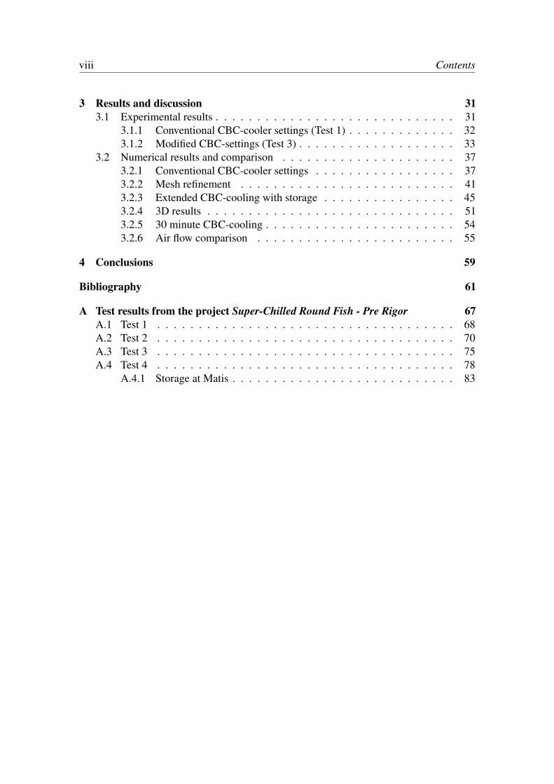
Contents
Preface iii
Abstract vi
1 Introduction 11.1 CBC-cooling of fillets . . . . . . . . . . . . . . . . . . . . . . . . . . . . 1
1.1.1 Storage Life . . . . . . . . . . . . . . . . . . . . . . . . . . . . . 31.2 CBC-cooling of whole fish . . . . . . . . . . . . . . . . . . . . . . . . . 41.3 Thesis Statement . . . . . . . . . . . . . . . . . . . . . . . . . . . . . . 5
2 Materials and methods 72.1 White fish properties . . . . . . . . . . . . . . . . . . . . . . . . . . . . 72.2 Temperature measurements . . . . . . . . . . . . . . . . . . . . . . . . . 102.3 Numerical modelling . . . . . . . . . . . . . . . . . . . . . . . . . . . . 14
2.3.1 Geometry . . . . . . . . . . . . . . . . . . . . . . . . . . . . . . 142.3.2 Mesh generation . . . . . . . . . . . . . . . . . . . . . . . . . . 192.3.3 Governing equations . . . . . . . . . . . . . . . . . . . . . . . . 212.3.4 Solution procedure . . . . . . . . . . . . . . . . . . . . . . . . . 232.3.5 Boundary conditions . . . . . . . . . . . . . . . . . . . . . . . . 252.3.6 Transient conduction . . . . . . . . . . . . . . . . . . . . . . . . 262.3.7 Thermal contact resistance . . . . . . . . . . . . . . . . . . . . . 262.3.8 Near wall treatment . . . . . . . . . . . . . . . . . . . . . . . . . 272.3.9 Error estimation . . . . . . . . . . . . . . . . . . . . . . . . . . . 29
vii
viii Contents
3 Results and discussion 313.1 Experimental results . . . . . . . . . . . . . . . . . . . . . . . . . . . . . 31
3.1.1 Conventional CBC-cooler settings (Test 1) . . . . . . . . . . . . . 323.1.2 Modified CBC-settings (Test 3) . . . . . . . . . . . . . . . . . . . 33
3.2 Numerical results and comparison . . . . . . . . . . . . . . . . . . . . . 373.2.1 Conventional CBC-cooler settings . . . . . . . . . . . . . . . . . 373.2.2 Mesh refinement . . . . . . . . . . . . . . . . . . . . . . . . . . 413.2.3 Extended CBC-cooling with storage . . . . . . . . . . . . . . . . 453.2.4 3D results . . . . . . . . . . . . . . . . . . . . . . . . . . . . . . 513.2.5 30 minute CBC-cooling . . . . . . . . . . . . . . . . . . . . . . . 543.2.6 Air flow comparison . . . . . . . . . . . . . . . . . . . . . . . . 55
4 Conclusions 59
Bibliography 61
A Test results from the project Super-Chilled Round Fish - Pre Rigor 67A.1 Test 1 . . . . . . . . . . . . . . . . . . . . . . . . . . . . . . . . . . . . 68A.2 Test 2 . . . . . . . . . . . . . . . . . . . . . . . . . . . . . . . . . . . . 70A.3 Test 3 . . . . . . . . . . . . . . . . . . . . . . . . . . . . . . . . . . . . 75A.4 Test 4 . . . . . . . . . . . . . . . . . . . . . . . . . . . . . . . . . . . . 78
A.4.1 Storage at Matis . . . . . . . . . . . . . . . . . . . . . . . . . . . 83
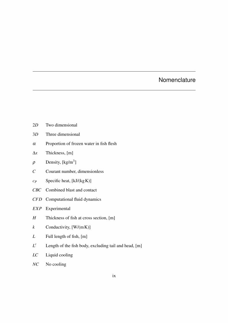
Nomenclature
2D Two dimensional
3D Three dimensional
α Proportion of frozen water in fish flesh
∆x Thickness, [m]
ρ Density, [kg/m3]
C Courant number, dimensionless
cP Specific heat, [kJ/(kgK)]
CBC Combined blast and contact
CFD Computational fluid dynamics
EXP Experimental
H Thickness of fish at cross section, [m]
k Conductivity, [W/(mK)]
L Full length of fish, [m]
L′ Length of the fish body, excluding tail and head, [m]
LC Liquid cooling
NC No cooling
ix
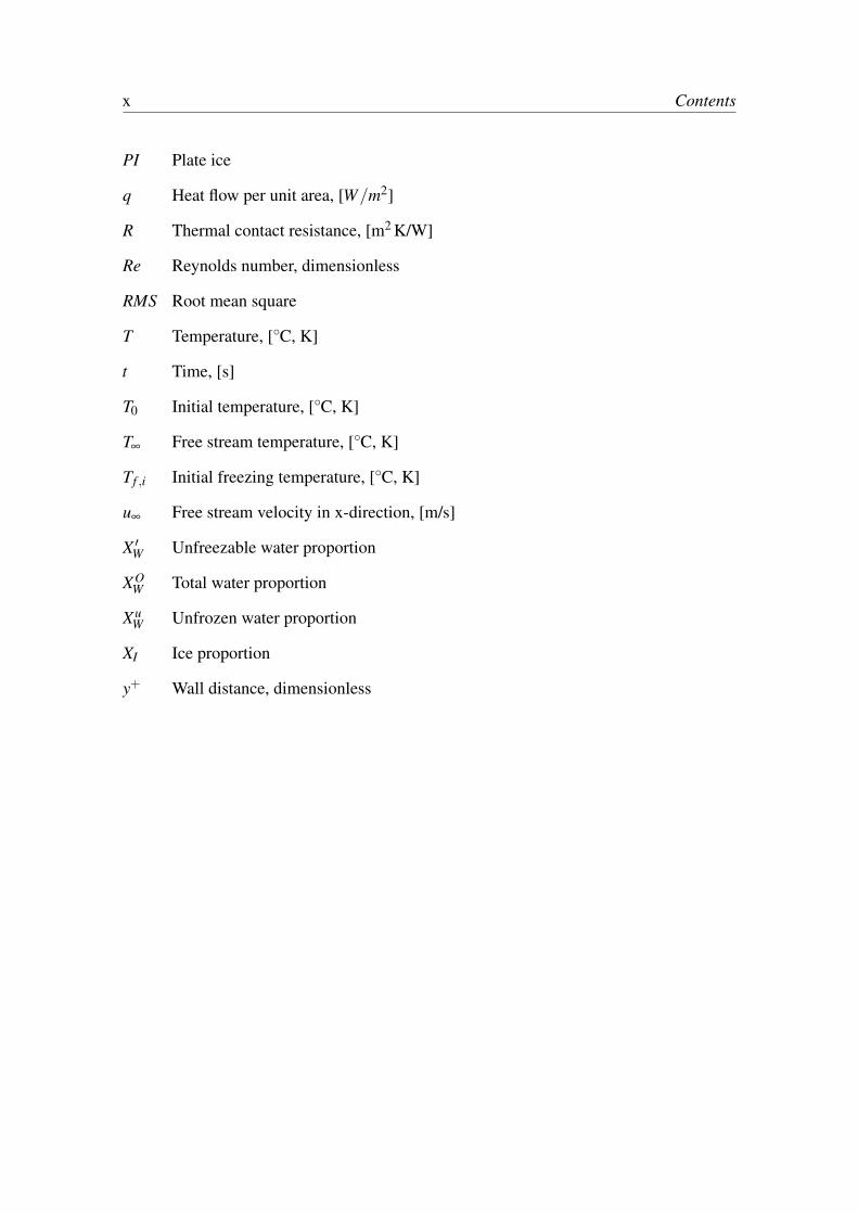
x Contents
PI Plate ice
q Heat flow per unit area, [W/m2]
R Thermal contact resistance, [m2 K/W]
Re Reynolds number, dimensionless
RMS Root mean square
T Temperature, [◦C, K]
t Time, [s]
T0 Initial temperature, [◦C, K]
T∞ Free stream temperature, [◦C, K]
Tf ,i Initial freezing temperature, [◦C, K]
u∞ Free stream velocity in x-direction, [m/s]
X ′W Unfreezable water proportion
XOW Total water proportion
XuW Unfrozen water proportion
XI Ice proportion
y+ Wall distance, dimensionless

CHAPTER 1
Introduction
Fish quality and hence, its value is mainly influenced by five factors: Handling, cooling,processing, packaging and storage. The storage life of fresh fish products is very limitedand is therefore an important factor to take into account when the product is to be exported.In order to maintain fish freshness during exportation, temperature control inside thestorage is very important. The Combined Blast and Contact (CBC) cooling method hasresulted in prolonged storage life of fish fillets [Lauzon et al., 2010] and possibly for wholefish [Gao, 2007].
1.1 CBC-cooling of filletsCBC-cooling is a processing technique developed by the company Skaginn ltd. (Akranes,Iceland). The technique is based on superchilling the product by transferring it through afreezer tunnel on a Teflon coated aluminium belt and simultaneously blasting cold air overit. The contact cooling is generated by the cooling energy accumulated in the aluminiumbelt. This cooling method which slightly freezes the skin in contact with the belt, withoutexcessively freezing the flesh, has mainly been applied for cooling fillets, not whole fish.Superchilling, as used for preservation of food, implies temperatures in the borderlinebetween chilling and freezing, i.e. slightly below the initial freezing point of the fish.
The CBC-cooling is considered a quick freezing process which results in good productquality. This is because food products in general contain a considerable amount of waterand when the product is considered frozen, most of its water content has been turned intoice. Slow freezing causes the formation of large ice crystals which might cause damage tothe cells in the biological material of the product. Quick freezing, such as the CBC-cooling,
1
2 1 Introduction
results in small ice crystal formation and less damage to the product [Granryd, 2005]. TheCBC-cooling delivers a stiff and robust product which makes cutting and trimming easier.Since the ice crystal formation is very small, its liquid remains inside the fish flesh. Theseadvantages result in a product of great quality with increased storage life compared toother methods [Magnússon et al., 2009]. The main challenge in this process is to maintaina stable and a sufficiently low temperature, which often is more difficult for fresh foodrather than frozen food.
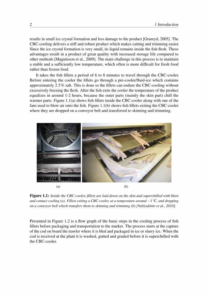
It takes the fish fillets a period of 6 to 8 minutes to travel through the CBC-cooler.Before entering the cooler the fillets go through a pre-cooler/fluid-ice which containsapproximately 2.5% salt. This is done so the fillets can endure the CBC-cooling withoutexcessively freezing the flesh. After the fish exits the cooler the temperature of the productequalizes in around 1-2 hours, because the outer parts (mainly the skin part) chill thewarmer parts. Figure 1.1(a) shows fish fillets inside the CBC-cooler along with one of thefans used to blow air onto the fish. Figure 1.1(b) shows fish fillets exiting the CBC-coolerwhere they are dropped on a conveyor belt and transferred to skinning and trimming.
(a) (b)
Figure 1.1: Inside the CBC-cooler, fillets are laid down on the skin and superchilled with blastand contact cooling (a). Fillets exiting a CBC-cooler, at a temperature around −1 ◦C, and droppingon a conveyor belt which transfers them to skinning and trimming (b) [Valtýsdóttir et al., 2010].
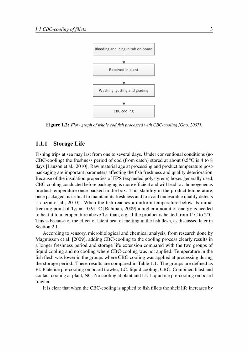
Presented in Figure 1.2 is a flow graph of the basic steps in the cooling process of fishfillets before packaging and transportation to the market. The process starts at the captureof the cod on board the trawler where it is bled and packaged in ice or slurry ice. When thecod is received at the plant it is washed, gutted and graded before it is superchilled withthe CBC-cooler.
1.1 CBC-cooling of fillets 3
Figure 1.2: Flow graph of whole cod fish processed with CBC-cooling [Gao, 2007].
1.1.1 Storage Life
Fishing trips at sea may last from one to several days. Under conventional conditions (noCBC-cooling) the freshness period of cod (from catch) stored at about 0.5◦C is 4 to 8days [Lauzon et al., 2010]. Raw material age at processing and product temperature post-packaging are important parameters affecting the fish freshness and quality deterioration.Because of the insulation properties of EPS (expanded polystyrene) boxes generally used,CBC-cooling conducted before packaging is more efficient and will lead to a homogeneousproduct temperature once packed in the box. This stability in the product temperature,once packaged, is critical to maintain its freshness and to avoid undesirable quality defects[Lauzon et al., 2010]. When the fish reaches a uniform temperature below its initialfreezing point of Tf,i = −0.91◦C [Rahman, 2009] a higher amount of energy is neededto heat it to a temperature above Tf,i than, e.g. if the product is heated from 1◦C to 2◦C.This is because of the effect of latent heat of melting in the fish flesh, as discussed later inSection 2.1.
According to sensory, microbiological and chemical analysis, from research done byMagnússon et al. [2009], adding CBC-cooling to the cooling process clearly results ina longer freshness period and storage life extension compared with the two groups ofliquid cooling and no cooling where CBC-cooling was not applied. Temperature in thefish flesh was lower in the groups where CBC-cooling was applied at processing duringthe storage period. These results are compared in Table 1.1. The groups are defined asPI: Plate ice pre-cooling on board trawler, LC: liquid cooling, CBC: Combined blast andcontact cooling at plant, NC: No cooling at plant and LI: Liquid ice pre-cooling on boardtrawler.
It is clear that when the CBC-cooling is applied to fish fillets the shelf life increases by
4 1 Introduction
3-4 days and the freshness period by 1-2 days compared with liquid cooling and no cooling.The comparison in Table 1.1 shows that the CBC-cooling is an important cooling techniquewhich can be used to gain and maintain the value of the product. The end of the freshnessperiod is defined as when the fish has lost the freshness characteristics and reached theneutral phase (Torry score 7 out of 10). The end of the maximum shelf life period is whenodour and flavour attributes (Torry score 5.5 out of 10) related to spoilage have becomeevident. The Torry scheme [Martinsdóttir et al., 2001] is used as an assessment of the fishflavour and odour with a scale from 1 to 10.
Table 1.1: Freshness period and shelf life from catch according to sensory evaluation. The codwas processed two days post-catch [Magnússon et al., 2009].
Group Freshness period Shelf lifePI, LC-CBC 6-8 days 14-15 days
PI, LC 6-7 days 9-12 daysPI, NC 5-8 days 8-11 days
LI, LC-CBC 8-9 days 15-16 days
Research performed by Martinsdóttir et al. [2004, 2005] showed that CBC-cooling slowsdown the deterioration process significantly compared with conventional processing. Byprocessing the the raw material one day from catch, a storage life of 13 days was obtainedfor cod fillets stored at 0.5◦C.
By working with the raw material three days from catch, a storage life of 14 days wasobtained for cod fillets stored in EPS boxes at 0.5◦C. Two days may be added to thisstorage life if the storage temperature is lowered from 0.5◦C to −1.5◦C [Olafsdóttir et al.,2006]. The storage temperature needs to be stable and close to −1.5◦C and −1.0◦C inorder to obtain the optimal storage for fish fillets.
Applying the CBC-cooling and storing the fish at 0.5◦C results in an overall sensoryshelf life of 12.5 to 14 days. When stored at −1.5◦C after the CBC-cooling, the storagelife is extended to at least 15 days. This shelf life extension is of high economical valuebecause it allows distant transportation of fresh fish by ship or truck, which is less expensivecompared to air freight [Olafsdóttir et al., 2006].
1.2 CBC-cooling of whole fishThe idea behind using the CBC-cooling technique on whole fish is to move the processshown in Figure 1.2 into the trawlers where the fish is caught. The largest amount ofinformation available about CBC-cooling of whole cod fish is found in research doneby Gao [2007]. In this research, CBC-cooling is compared with pre-cooling with slurryice and usage of cooling mats/packs. The cooling time of the CBC-cooler was fixed
1.3 Thesis Statement 5
at 11 minutes for all experiments. Two sets of experiments were made where differenttemperature settings were applied.
From the first experiment, conducted on December 8th, it was recommended that thecooling time of 11 minutes should be extended to decrease the central temperature down to−1◦C and that the air temperature should be in the range of −20◦C to −10◦C for wholecod with average weight around 1 kg.
From the second experiments, conducted on January 30th, it was concluded that anapproximate air temperature should be in the range of −23◦C to −20◦C for whole codwith an average weight around 1 kg, when cooled in a CBC-cooler for 11 minutes. Adifferent chilling time would result in different temperatures.
Results where CBC pre-cooling is compared with slurry ice and the use of coolingmats/packs show that CBC-cooling is a good method for delaying quality deteriorationof fresh cod fillets with regards to chemical and microbiological assessments. Carefultemperature monitoring in further chilled storage should be maintained to guarantee thefresh fish quality [Gao, 2007].
1.3 Thesis StatementThe main purpose of this work is two fold: (1) Conduct experiments to determine therequired setting in the CBC-cooler which cause superchilling of the flesh for whole fish,and (2) to generate CFD models in 2D and 3D to simulate the temperature behaviourinside a whole cod fish during CBC-cooling and the storage time. The simulated resultsare compared with experimental results. Results and settings used in this model canbe implemented for future simulations involving the CBC-cooling method, e.g. whenintroducing other fish species, such as salmon or when predicting longer cooling periods.

CHAPTER 2
Materials and methods
In this chapter the materials and methods used in the study are described. Firstly thethermal properties of white fish are presented, i.e. how the thermal conductivity andspecific heat vary with temperature. Secondly temperature measurements are describedby describing the placement of temperature data loggers inside and outside of the fishflesh along with the position of the anemometer used for recording air velocity inside theCBC-cooler. Lastly the theory and boundary conditions used for calculating the solutionare presented.
2.1 White fish propertiesWhen predicting the time necessary for cooling or heating of food products, informationon its thermal properties are of high importance. In order to obtain superchilling of theproduct, its core temperature must get below the products initial freezing temperature, Tf ,i.The fish product examined in this thesis is cod (Gadus morhua), which is one type of whitefish.
The initial freezing temperature(Tf ,i)
of cod is listed as −0.91◦C by Fikiin [1998]. Inresearch done by Margeirsson et al. [2012] a value of T f ,i = −0.92◦C was adopted in theFLUENT models because of a better fit with experimental data. The same value of Tf ,iis adopted in this study. When a product is cooled below its initial freezing temperature(Tf ,i), phase change of the water inside the fish muscle begins along with formation of icecrystals. According to Fikiin [1998] the total proportion of water within the fish flesh is80.3%.
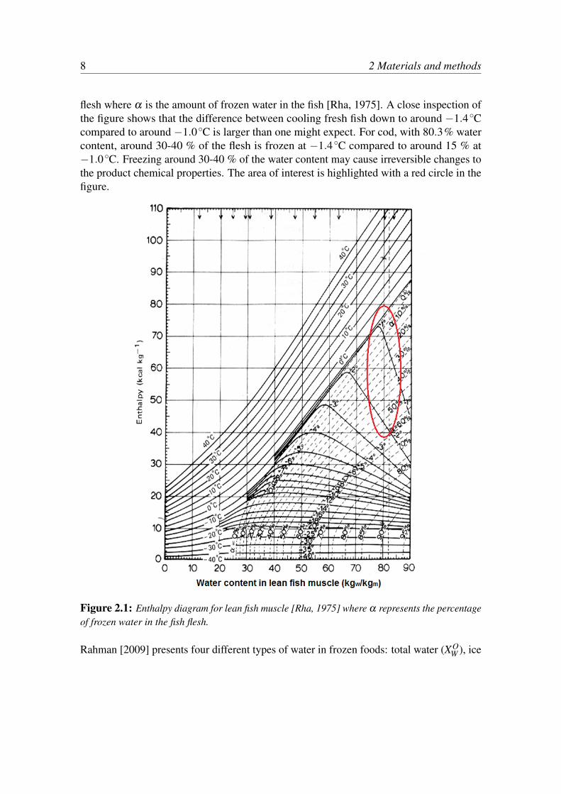
Figure 2.1 presents enthalpy as a function of the total amount of water within the fish
7
8 2 Materials and methods
flesh where α is the amount of frozen water in the fish [Rha, 1975]. A close inspection ofthe figure shows that the difference between cooling fresh fish down to around −1.4◦Ccompared to around −1.0◦C is larger than one might expect. For cod, with 80.3% watercontent, around 30-40 % of the flesh is frozen at −1.4◦C compared to around 15 % at−1.0◦C. Freezing around 30-40 % of the water content may cause irreversible changes tothe product chemical properties. The area of interest is highlighted with a red circle in thefigure.
Figure 2.1: Enthalpy diagram for lean fish muscle [Rha, 1975] where α represents the percentageof frozen water in the fish flesh.
Rahman [2009] presents four different types of water in frozen foods: total water (XOW ), ice
2.1 White fish properties 9
(XI), unfreezable water (X ′W ) and unfrozen water (XuW ). Total water can be written as
XOW = Xu
W +XI +X ′W (2.1.1)
Since not all water in the product is freezable, a good prediction for the amount of icecontent is achieved by
XI =(
XOW −X ′W
)(1−
Tf ,i
T
)(2.1.2)
with Tf ,i =−0.91◦C and(XO
W −X ′W)
as the total freezable water. Unfreezable water,expressed in kilograms of unfreezable water per kilogram of sample or dry solids, isdefined as:
X ′W = B(
1−XOW
)(2.1.3)
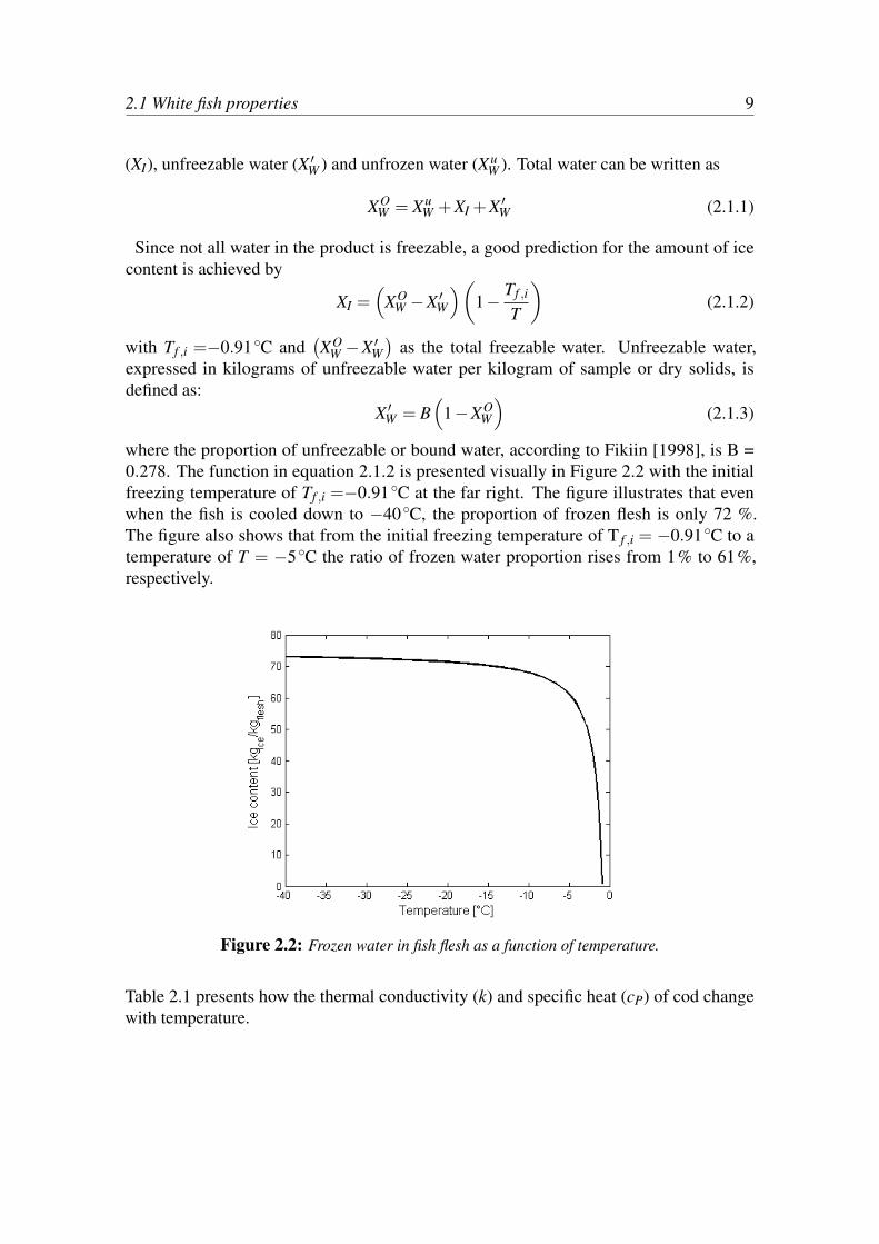
where the proportion of unfreezable or bound water, according to Fikiin [1998], is B =0.278. The function in equation 2.1.2 is presented visually in Figure 2.2 with the initialfreezing temperature of Tf ,i =−0.91◦C at the far right. The figure illustrates that evenwhen the fish is cooled down to −40◦C, the proportion of frozen flesh is only 72 %.The figure also shows that from the initial freezing temperature of T f ,i = −0.91◦C to atemperature of T = −5◦C the ratio of frozen water proportion rises from 1% to 61%,respectively.
Figure 2.2: Frozen water in fish flesh as a function of temperature.
Table 2.1 presents how the thermal conductivity (k) and specific heat (cP) of cod changewith temperature.
10 2 Materials and methods
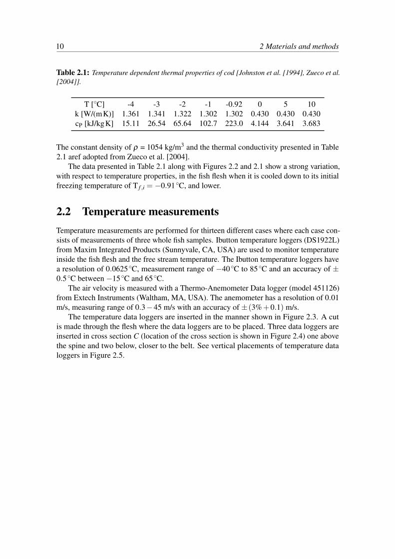
Table 2.1: Temperature dependent thermal properties of cod [Johnston et al. [1994], Zueco et al.[2004]].
T [◦C] -4 -3 -2 -1 -0.92 0 5 10k [W/(mK)] 1.361 1.341 1.322 1.302 1.302 0.430 0.430 0.430cP [kJ/kgK] 15.11 26.54 65.64 102.7 223.0 4.144 3.641 3.683
The constant density of ρ = 1054 kg/m3 and the thermal conductivity presented in Table2.1 aref adopted from Zueco et al. [2004].
The data presented in Table 2.1 along with Figures 2.2 and 2.1 show a strong variation,with respect to temperature properties, in the fish flesh when it is cooled down to its initialfreezing temperature of T f ,i = −0.91◦C, and lower.
2.2 Temperature measurementsTemperature measurements are performed for thirteen different cases where each case con-sists of measurements of three whole fish samples. Ibutton temperature loggers (DS1922L)from Maxim Integrated Products (Sunnyvale, CA, USA) are used to monitor temperatureinside the fish flesh and the free stream temperature. The Ibutton temperature loggers havea resolution of 0.0625◦C, measurement range of −40◦C to 85◦C and an accuracy of ±0.5◦C between −15◦C and 65◦C.
The air velocity is measured with a Thermo-Anemometer Data logger (model 451126)from Extech Instruments (Waltham, MA, USA). The anemometer has a resolution of 0.01m/s, measuring range of 0.3−45 m/s with an accuracy of ±(3%+0.1) m/s.
The temperature data loggers are inserted in the manner shown in Figure 2.3. A cutis made through the flesh where the data loggers are to be placed. Three data loggers areinserted in cross section C (location of the cross section is shown in Figure 2.4) one abovethe spine and two below, closer to the belt. See vertical placements of temperature dataloggers in Figure 2.5.
2.2 Temperature measurements 11
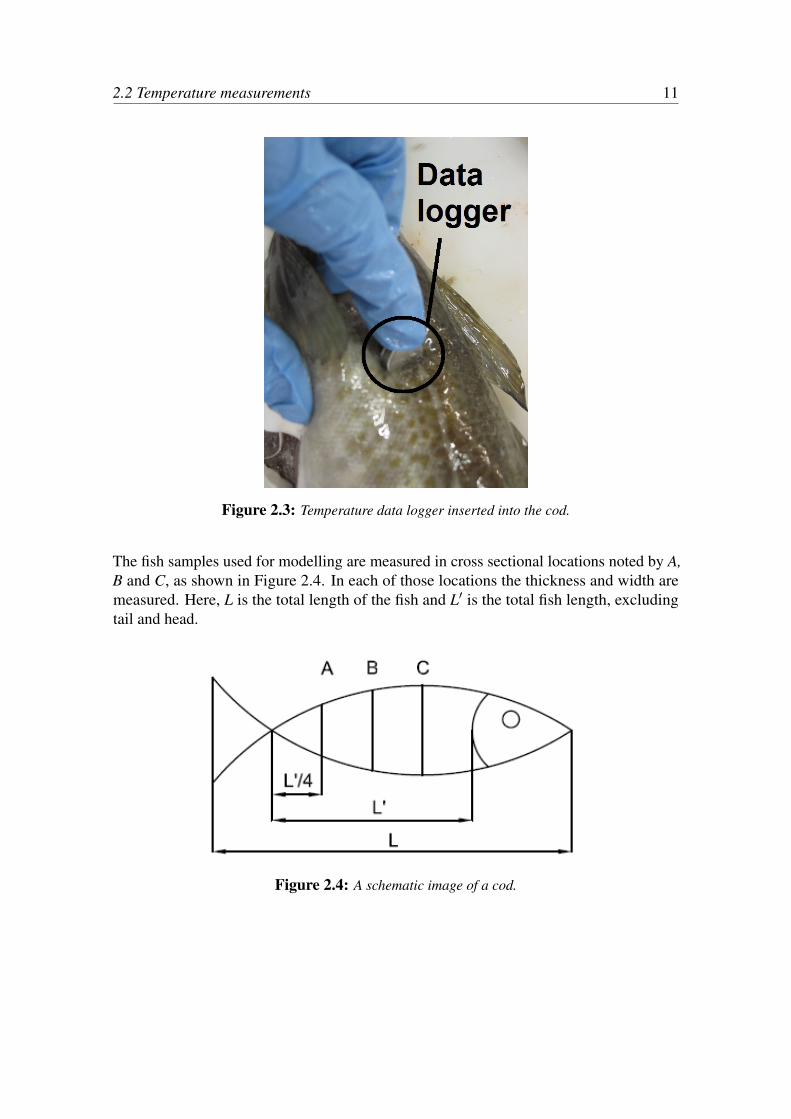
Figure 2.3: Temperature data logger inserted into the cod.
The fish samples used for modelling are measured in cross sectional locations noted by A,B and C, as shown in Figure 2.4. In each of those locations the thickness and width aremeasured. Here, L is the total length of the fish and L′ is the total fish length, excludingtail and head.
Figure 2.4: A schematic image of a cod.
12 2 Materials and methods
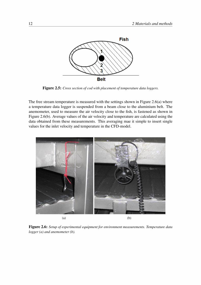
Figure 2.5: Cross section of cod with placement of temperature data loggers.
The free stream temperature is measured with the settings shown in Figure 2.6(a) wherea temperature data logger is suspended from a beam close to the aluminium belt. Theanemometer, used to measure the air velocity close to the fish, is fastened as shown inFigure 2.6(b). Average values of the air velocity and temperature are calculated using thedata obtained from these measurements. This averaging mae it simple to insert singlevalues for the inlet velocity and temperature in the CFD-model.
(a) (b)
Figure 2.6: Setup of experimental equipment for environment measurements. Temperature datalogger (a) and anemometer (b).
2.2 Temperature measurements 13
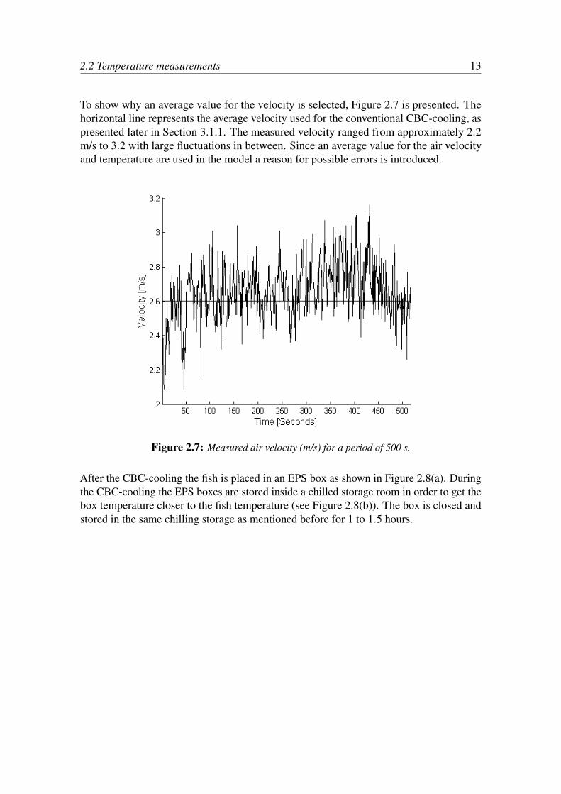
To show why an average value for the velocity is selected, Figure 2.7 is presented. Thehorizontal line represents the average velocity used for the conventional CBC-cooling, aspresented later in Section 3.1.1. The measured velocity ranged from approximately 2.2m/s to 3.2 with large fluctuations in between. Since an average value for the air velocityand temperature are used in the model a reason for possible errors is introduced.
Figure 2.7: Measured air velocity (m/s) for a period of 500 s.
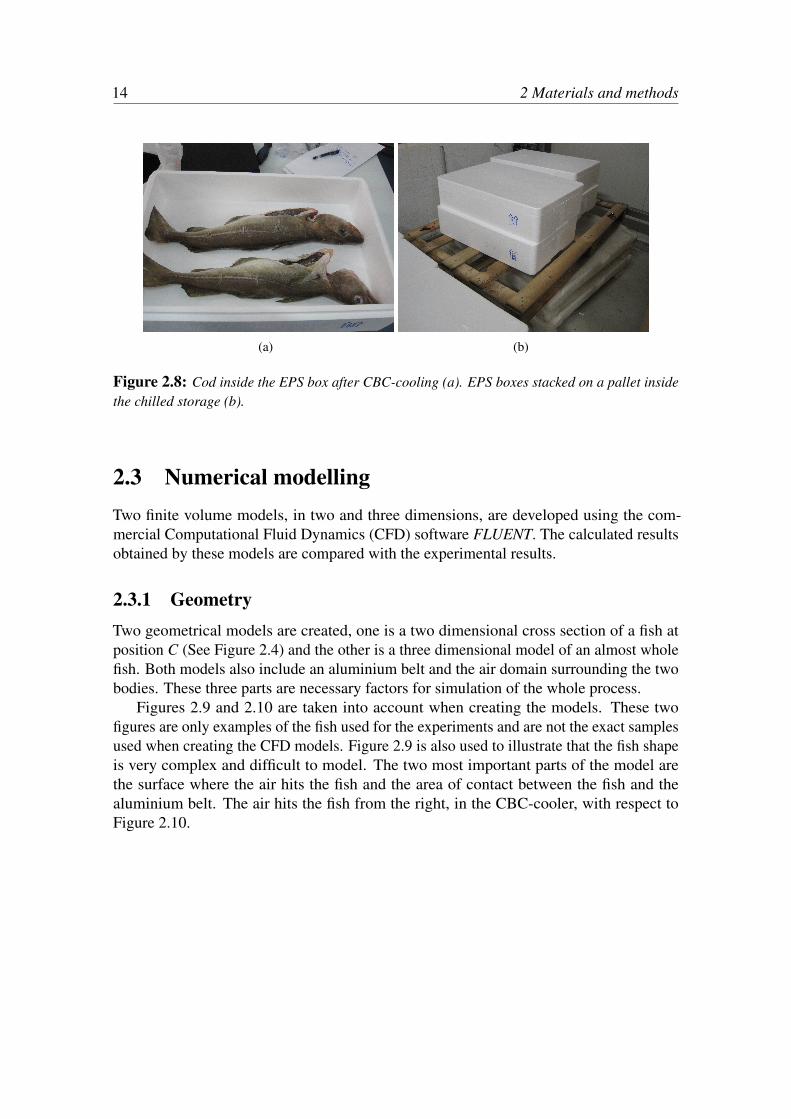
After the CBC-cooling the fish is placed in an EPS box as shown in Figure 2.8(a). Duringthe CBC-cooling the EPS boxes are stored inside a chilled storage room in order to get thebox temperature closer to the fish temperature (see Figure 2.8(b)). The box is closed andstored in the same chilling storage as mentioned before for 1 to 1.5 hours.
14 2 Materials and methods
(a) (b)
Figure 2.8: Cod inside the EPS box after CBC-cooling (a). EPS boxes stacked on a pallet insidethe chilled storage (b).
2.3 Numerical modellingTwo finite volume models, in two and three dimensions, are developed using the com-mercial Computational Fluid Dynamics (CFD) software FLUENT. The calculated resultsobtained by these models are compared with the experimental results.
2.3.1 GeometryTwo geometrical models are created, one is a two dimensional cross section of a fish atposition C (See Figure 2.4) and the other is a three dimensional model of an almost wholefish. Both models also include an aluminium belt and the air domain surrounding the twobodies. These three parts are necessary factors for simulation of the whole process.
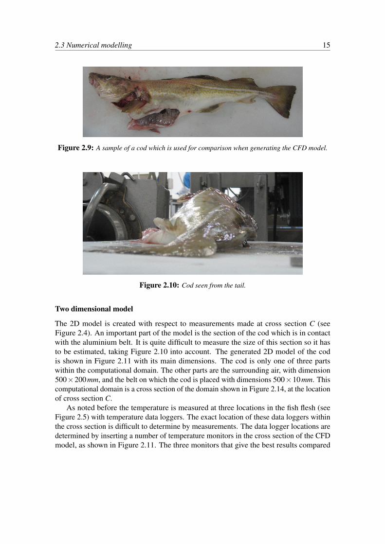
Figures 2.9 and 2.10 are taken into account when creating the models. These twofigures are only examples of the fish used for the experiments and are not the exact samplesused when creating the CFD models. Figure 2.9 is also used to illustrate that the fish shapeis very complex and difficult to model. The two most important parts of the model arethe surface where the air hits the fish and the area of contact between the fish and thealuminium belt. The air hits the fish from the right, in the CBC-cooler, with respect toFigure 2.10.
2.3 Numerical modelling 15
Figure 2.9: A sample of a cod which is used for comparison when generating the CFD model.
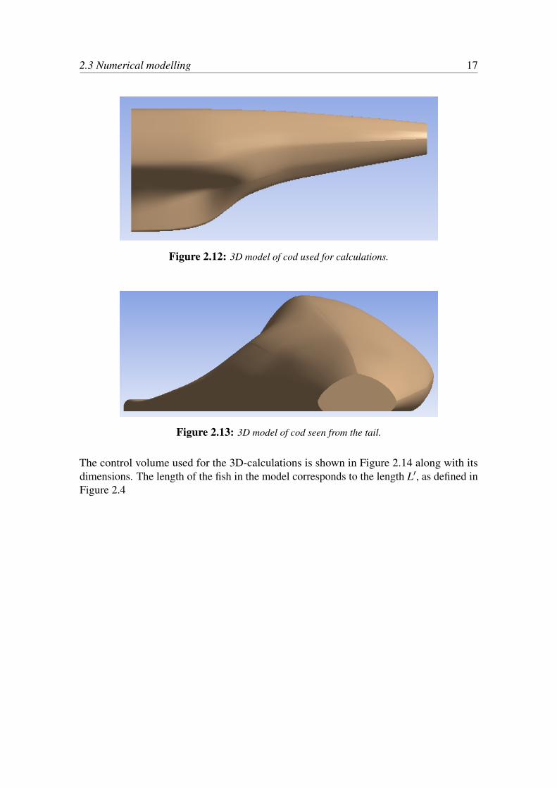
Figure 2.10: Cod seen from the tail.
Two dimensional model
The 2D model is created with respect to measurements made at cross section C (seeFigure 2.4). An important part of the model is the section of the cod which is in contactwith the aluminium belt. It is quite difficult to measure the size of this section so it hasto be estimated, taking Figure 2.10 into account. The generated 2D model of the codis shown in Figure 2.11 with its main dimensions. The cod is only one of three partswithin the computational domain. The other parts are the surrounding air, with dimension500×200 mm, and the belt on which the cod is placed with dimensions 500×10 mm. Thiscomputational domain is a cross section of the domain shown in Figure 2.14, at the locationof cross section C.
As noted before the temperature is measured at three locations in the fish flesh (seeFigure 2.5) with temperature data loggers. The exact location of these data loggers withinthe cross section is difficult to determine by measurements. The data logger locations aredetermined by inserting a number of temperature monitors in the cross section of the CFDmodel, as shown in Figure 2.11. The three monitors that give the best results compared

16 2 Materials and methods
with experiments are used in comparison. It should be noted that the position of thesemonitors vary for different fish specimen since the data logger locations within each fishare never exactly the same.
Figure 2.11: 2D model of the cod with dimensions (mm) and placement of temperature monitors.
The temperature from each monitor is stored after a pre-defined number of time stepsand written in a .out file which is used for post-processing. The temperature values areobtained by applying a vertex average to each cell. The vertex average of a specified fieldvariable on a surface is computed by dividing the summation of the vertex values of theselected variable by the total number of vertices [ANSYS, 2009].
Three dimensional model
The main reason for making the model in 3D is to see if the thickness variations alongthe length of the cod (z-direction) result in different effects on the temperature gradientsin cross section C compared with the 2D model. The height and width measurements ofcross sections A, B and C and the measured lengths between the cross sections (L’/4) areused to produce a 3D model. The 3D model is generated by using the Loft feature wherethe geometry of a number of aligned cross sections are used to create a solid body. Thegenerated geometry is shown in Figures 2.12 and 2.13.
2.3 Numerical modelling 17
Figure 2.12: 3D model of cod used for calculations.
Figure 2.13: 3D model of cod seen from the tail.
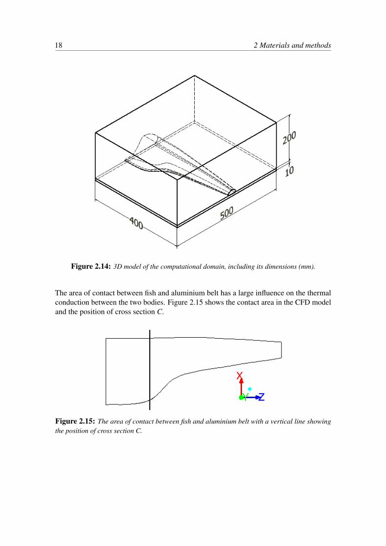
The control volume used for the 3D-calculations is shown in Figure 2.14 along with itsdimensions. The length of the fish in the model corresponds to the length L′, as defined inFigure 2.4
18 2 Materials and methods
Figure 2.14: 3D model of the computational domain, including its dimensions (mm).
The area of contact between fish and aluminium belt has a large influence on the thermalconduction between the two bodies. Figure 2.15 shows the contact area in the CFD modeland the position of cross section C.
Figure 2.15: The area of contact between fish and aluminium belt with a vertical line showingthe position of cross section C.
2.3 Numerical modelling 19
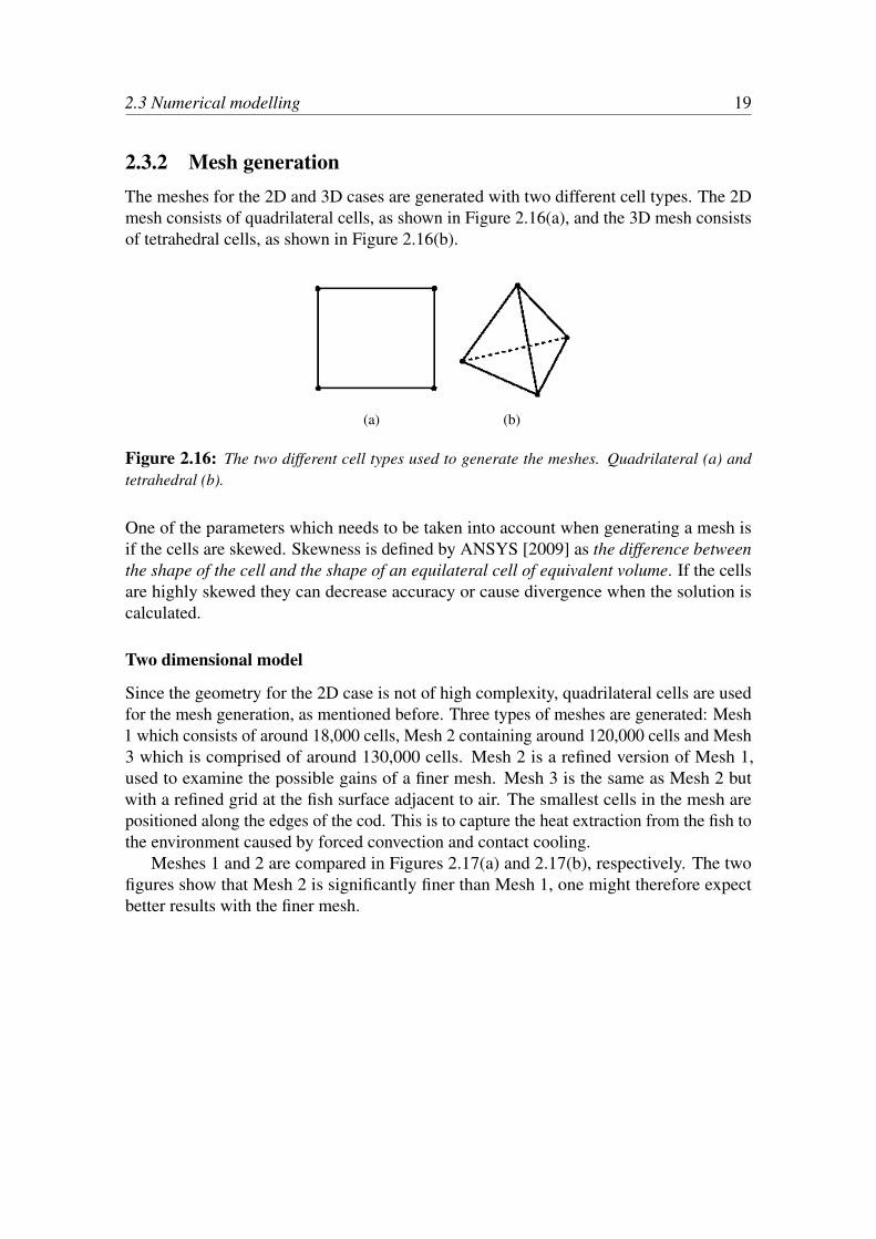
2.3.2 Mesh generationThe meshes for the 2D and 3D cases are generated with two different cell types. The 2Dmesh consists of quadrilateral cells, as shown in Figure 2.16(a), and the 3D mesh consistsof tetrahedral cells, as shown in Figure 2.16(b).
(a) (b)
Figure 2.16: The two different cell types used to generate the meshes. Quadrilateral (a) andtetrahedral (b).
One of the parameters which needs to be taken into account when generating a mesh isif the cells are skewed. Skewness is defined by ANSYS [2009] as the difference betweenthe shape of the cell and the shape of an equilateral cell of equivalent volume. If the cellsare highly skewed they can decrease accuracy or cause divergence when the solution iscalculated.
Two dimensional model
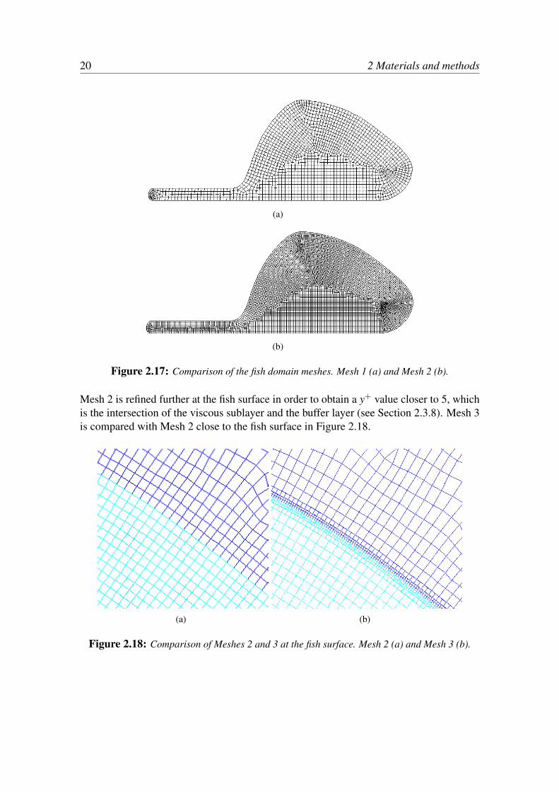
Since the geometry for the 2D case is not of high complexity, quadrilateral cells are usedfor the mesh generation, as mentioned before. Three types of meshes are generated: Mesh1 which consists of around 18,000 cells, Mesh 2 containing around 120,000 cells and Mesh3 which is comprised of around 130,000 cells. Mesh 2 is a refined version of Mesh 1,used to examine the possible gains of a finer mesh. Mesh 3 is the same as Mesh 2 butwith a refined grid at the fish surface adjacent to air. The smallest cells in the mesh arepositioned along the edges of the cod. This is to capture the heat extraction from the fish tothe environment caused by forced convection and contact cooling.
Meshes 1 and 2 are compared in Figures 2.17(a) and 2.17(b), respectively. The twofigures show that Mesh 2 is significantly finer than Mesh 1, one might therefore expectbetter results with the finer mesh.
20 2 Materials and methods
(a)
(b)
Figure 2.17: Comparison of the fish domain meshes. Mesh 1 (a) and Mesh 2 (b).
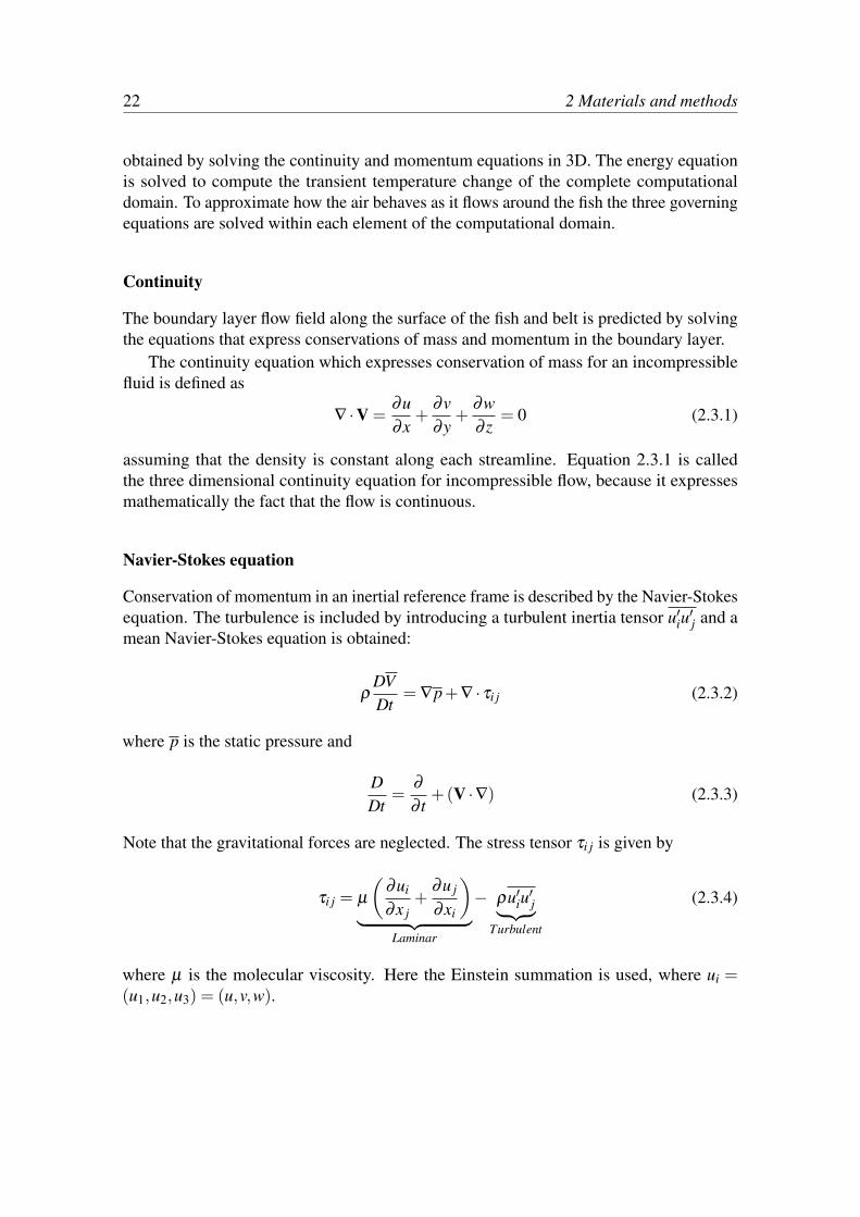
Mesh 2 is refined further at the fish surface in order to obtain a y+ value closer to 5, whichis the intersection of the viscous sublayer and the buffer layer (see Section 2.3.8). Mesh 3is compared with Mesh 2 close to the fish surface in Figure 2.18.
(a) (b)
Figure 2.18: Comparison of Meshes 2 and 3 at the fish surface. Mesh 2 (a) and Mesh 3 (b).

2.3 Numerical modelling 21
Three dimensional model
The 3D case consists of a semi-full fish model which is complex in shape. It is thereforenot the best option to use a mesh of quadrilateral cells. The selected cells for this case aretetrahedral which are easily adjusted to the defined geometry. The 3D mesh of the fish,seen from above, is presented in Figure 2.19. The whole computational domain consistsof a total of approximately 1,345,000 elements which is significantly higher than for thefinest 2D mesh (Mesh 3).
Figure 2.19: Mesh of the 3D model seen from above.
A cross section of the mesh in 3D is shown in Figure 2.20. When this cross section iscompared with the 2D cross section of Mesh 2 (see Figure 2.17(b)), it is clear that the2D mesh is finer. The 3D mesh might therefore not return results as accurate as the 2Dmeshes. The main purpose of the 3D case is to see if there are any longitudinal coolingeffects obtained in the fish flesh.
Figure 2.20: Mesh of the 3D model seen from the fish head.
2.3.3 Governing equationsThis section introduces the governing equations used to solve the fluid flow and heattransfer inside the computational domain. The flow field behaviour in the models is
22 2 Materials and methods
obtained by solving the continuity and momentum equations in 3D. The energy equationis solved to compute the transient temperature change of the complete computationaldomain. To approximate how the air behaves as it flows around the fish the three governingequations are solved within each element of the computational domain.
Continuity
The boundary layer flow field along the surface of the fish and belt is predicted by solvingthe equations that express conservations of mass and momentum in the boundary layer.
The continuity equation which expresses conservation of mass for an incompressiblefluid is defined as
∇ ·V =∂u∂x
+∂v∂y
+∂w∂ z
= 0 (2.3.1)
assuming that the density is constant along each streamline. Equation 2.3.1 is calledthe three dimensional continuity equation for incompressible flow, because it expressesmathematically the fact that the flow is continuous.
Navier-Stokes equation
Conservation of momentum in an inertial reference frame is described by the Navier-Stokesequation. The turbulence is included by introducing a turbulent inertia tensor u′iu
′j and a
mean Navier-Stokes equation is obtained:
ρDVDt
= ∇p+∇ · τi j (2.3.2)
where p is the static pressure and
DDt
=∂
∂ t+(V ·∇) (2.3.3)
Note that the gravitational forces are neglected. The stress tensor τi j is given by
τi j = µ
(∂ui
∂x j+
∂u j
∂xi
)︸ ︷︷ ︸
Laminar
− ρu′iu′j︸ ︷︷ ︸
Turbulent
(2.3.4)
where µ is the molecular viscosity. Here the Einstein summation is used, where ui =(u1,u2,u3) = (u,v,w).
2.3 Numerical modelling 23
Energy equation
By applying the law of conservation of energy and the Fourier’s law of heat conductionon a differential volume and taking the limiting case of this as volume goes to zero, onearrives at the general equation for thermal energy transport, defined as:
ρcPDTDt
=− ∂
∂xi(qi)+Φ (2.3.5)
where
Φ =µ
2
(∂ui
∂x j+
∂u′i∂x j
+∂u j
∂xi+
∂u′j∂xi
)2
(2.3.6)
and
qi =−k∂T∂xi︸ ︷︷ ︸
Laminar
+ρcpu′iT ′︸ ︷︷ ︸Turbulent
(2.3.7)
The velocities u,v and w can be obtained by solving Equation 2.3.2 [White, 2006]. Notethat within the fish cross section the specific heat, cp, and conductivity, k, are functions oftemperature as defined in Section 2.1.
The equations of continuity, momentum and energy can be made dimensionless byredefining the dependent and independent variables as dimensionless. This is done bydividing the variables by constant reference properties which apply for the flow. Bysubstitution of these dimensionless numbers into the energy equation and rearranging theequation, one of the dimensionless parameters obtained is the Reynolds number. Thesame number is obtained by substituting dimensionless parameters into the Navier-Stokesequation [White, 2006]. The Reynolds number is defined as:
Re =H u∞
ν(2.3.8)
Here, the length parameter H is the height of the fish at cross section C, as defined in Figure2.11. With the air inlet velocity, u∞ = 2.6 m/s and the kinematic viscosity at −7.4◦C as ν
= 1.26 × 10⁻⁵ m2/s a Reynolds number of 13,000 is obtained. According to Lienhard IVand Lienhard V [2010] turbulent behaviour for a circular cylinder in cross flow occursfor values of Re above 150. Since, in this case, Re = 13,000 the air flow is consideredturbulent.
2.3.4 Solution procedureThe solution obtained by the commercial CFD code FLUENT is solved using a pressurebased solver. The pressure based solver uses an algorithm where mass conservation of thevelocity field is achieved by solving a pressure equation. The pressure equation is derived
24 2 Materials and methods
from the continuity and momentum equations so that the velocity field, corrected by thepressure, satisfies continuity. The governing equations are non-linear and coupled to oneanother. Hence, a solution is obtained by iterating the entire set of governing equationsuntil convergence is obtained [ANSYS, 2009, p. 642].
FLUENT converts the general scalar transport equation to an algebraic equation whichcan be solved numerically by using the finite volume technique. This technique involvesapproximating the integral with a sum and using interpolation to obtain the required facevalue.
Discretisation of the governing equations on a given two dimensional triangular cell,for a scalar quantity, φ , may be expressed as
∂ρφ
∂ tV +
N f aces
∑f
ρ f~v f φ f ·~A =N f aces
∑f
φ ∇φ f ·~A f +SφV (2.3.9)
where N f aces is the number of faces enclosing the cell, φ f is the face value of φ , ρ f~v f ·~Ais the mass flux through the face, ~A is the face area, ∇φ f is the gradient of φ at the face
and V is the cell volume. The time dependent value of∂ρφ
∂ tV is a part of the temporal
discretisation.
Spatial discretisation
By default FLUENT stores discrete values of the scalar, φ , at the center of each cell. Inorder to determine the convection terms in Equation 2.3.9, face values (φ f ) are requiredand must be interpolated from the cell center values. This is done by using an upwindscheme, or in this study a second order upwind scheme.
Upwind means that the face value φ f is determined from cell values that are upstreamwith regards to the direction of the normal velocity vn (see Equation 2.3.9). Since highaccuracy is preferred to the solution, a second order upwind scheme is selected. Thisscheme computes cell face quantities by applying a multidimensional linear reconstructionwhich uses a Taylor series expansion to achieve high-order accuracy. The face value, φ f , iscomputed using the following expression:
φ f = φ +∇φ ·~r (2.3.10)
where φ and ∇φ are the cell-centered value and its gradient in the upstream cell and~r is thedistance from the upstream centroid to the face centroid. The gradient ∇φ is determinedby the Least squares cell-based method where the solution is assumed to vary linearly.
Temporal discretisation
Discretisation of the governing equations (Equations 2.3.1 to 2.3.5) in both space and timeis very important for transient simulations. When the temporal discretisation is applied, the
2.3 Numerical modelling 25
differential equations are integrated over a time step ∆t. The time derivative is discretisedby using second order discretisation.
The governing equations are linearised in the CFD code either in an implicit or explicitform. For the implicit form, which is selected in this case, the unknown value in each cellfor a given variable, is computed where relation between known and unknown values fromthe neighbouring cells are used. Each unknown value will therefore appear in more thanone equation in the system. To get a solution these equations must be solved simultaneouslyby iteration [ANSYS, 2009, p. 641-673].
The time step, ∆t, used when calculating the solution needs to be adjusted with respectto the dimensionless Courant number in the fluid domain. The Courant number is definedas
C =∆t ·u∞
∆xcell(2.3.11)
where ∆xcell is the width of the smallest fluid cell and u∞ is the free stream fluid velocityin the x-direction.
The system, which is solved with an implicit solver, requires that, for a stable andefficient calculation, the Courant number should not exceed a value of 20-40 in the mostsensitive regions of the domain [ANSYS, 2009]. Looking at Equation 2.3.11 one can seethat when the the mesh is refined the time step needs to be decreased to a value accordingto the width of the smallest fluid cell.
2.3.5 Boundary conditions
In order to generate good results, which show a good comparison, appropriate boundaryconditions must be applied to the computational domain. The most important settings,such as the inlet velocity, the initial temperature and the air temperature, are obtained bymeasurements as described in Section 2.2.
The fish is assumed to be at uniform initial temperature, T0. The air flow is consideredincompressible and uniform at the inlet of the control volume, representing the fans blowingin the air. The air temperature at the inlet is considered constant and expressed with T∞.Under real circumstances the temperature and velocity fluctuate during the cooling period(see Figure 2.7).
Since the CBC-cooling is a low temperature process which takes place within a closedspace, radiation effects are neglected.
The boundary conditions at the outlet and top wall of the control volume are set aspressure outlets with a constant temperature of T∞. A turbulence intensity of 10 % and alength scale of 1 cm is used within the fluid domain.
A coupled boundary condition is applied between the air and fish surface, as well asbetween the air and belt. This boundary condition allows interaction between the fluid andsolid zones, or in this case heat transfer.
26 2 Materials and methods
The 2D model is in fact a 3D model with symmetric boundary conditions at the viewplanes. The 2D model, therefore, simulates a fish with uniform thickness out of and intothe view plane. This means that the effect of thickness and geometry change along the fishhas no influence on the solution.
The solution for the modified CBC-cooler settings is calculated in two parts in FLUENT.The modified CBC-cooling conditions are applied for a period of 14 minutes. After theCBC-cooling the air flow is cut off and set to 0 m/s and adiabatic boundary conditions (noheat flux) are applied to the four surrounding walls because the good insulation of the EPSbox.
2.3.6 Transient conductionTransient conduction is defined as the mode of thermal energy flow within an object, inwhich temperatures change in time. During the transient conduction period, temperatureswithin the system will change in time towards a new equilibrium. Once equilibrium isreached, heat flow into the system will equal the heat flow out, and temperatures at eachpoint inside the system no longer change. At this point, transient conduction has ended,although steady-state conduction may continue if the heat flow continues [Lienhard IVand Lienhard V, 2010]. This definition describes the process of CBC-cooling in a goodmanner and is therefore applied to the CFD model.
In the cases presented in this thesis, steady-state is not reached during the time ofCBC-cooling. After the CBC-cooling the fish is placed in an EPS-box where it is stored forapproximately one hour. During this storage period the system reaches conditions whichare very close to steady state where the fish temperature is almost uniform. Temperatureclose to the fish center continues to get lower during the storage because the skin is so coldthat it keeps extracting heat from inside the fish until it reaches equilibrium. This processmight take up to two hours of storage time.
2.3.7 Thermal contact resistanceThe actual temperature profile through two materials in contact results in a temperaturedrop between the bodies. The temperature drop in the contact plane between the twomaterials is said to be the result of thermal contact resistance.
No real surface is perfectly smooth, and the actual surface roughness is believed to playa central role in determining the contact resistance. Two factors are of most importancewhen examining heat transfer at the joints: a) The solid-to-solid conduction at the spotsof contact, and b) The conduction through entrapped gases in the void spaces created bythe contact. Factor b) is assumed to represent the major resistance to heat flow, since thethermal conductivity of the gas is quite small compared to the solids [Holman, 2010].
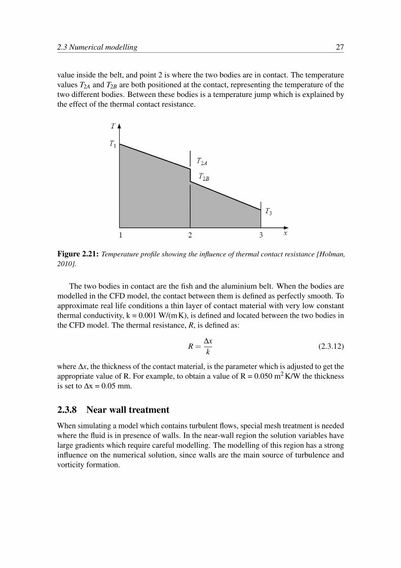
The temperature profile between two solid materials with a thermal contact resistance ispresented in Figure 2.21. Here T1 is a temperature value inside the fish, T3 is a temperature
2.3 Numerical modelling 27
value inside the belt, and point 2 is where the two bodies are in contact. The temperaturevalues T2A and T2B are both positioned at the contact, representing the temperature of thetwo different bodies. Between these bodies is a temperature jump which is explained bythe effect of the thermal contact resistance.
Figure 2.21: Temperature profile showing the influence of thermal contact resistance [Holman,2010].
The two bodies in contact are the fish and the aluminium belt. When the bodies aremodelled in the CFD model, the contact between them is defined as perfectly smooth. Toapproximate real life conditions a thin layer of contact material with very low constantthermal conductivity, k = 0.001 W/(mK), is defined and located between the two bodies inthe CFD model. The thermal resistance, R, is defined as:
R =∆xk
(2.3.12)
where ∆x, the thickness of the contact material, is the parameter which is adjusted to get theappropriate value of R. For example, to obtain a value of R = 0.050 m2 K/W the thicknessis set to ∆x = 0.05 mm.
2.3.8 Near wall treatmentWhen simulating a model which contains turbulent flows, special mesh treatment is neededwhere the fluid is in presence of walls. In the near-wall region the solution variables havelarge gradients which require careful modelling. The modelling of this region has a stronginfluence on the numerical solution, since walls are the main source of turbulence andvorticity formation.
28 2 Materials and methods
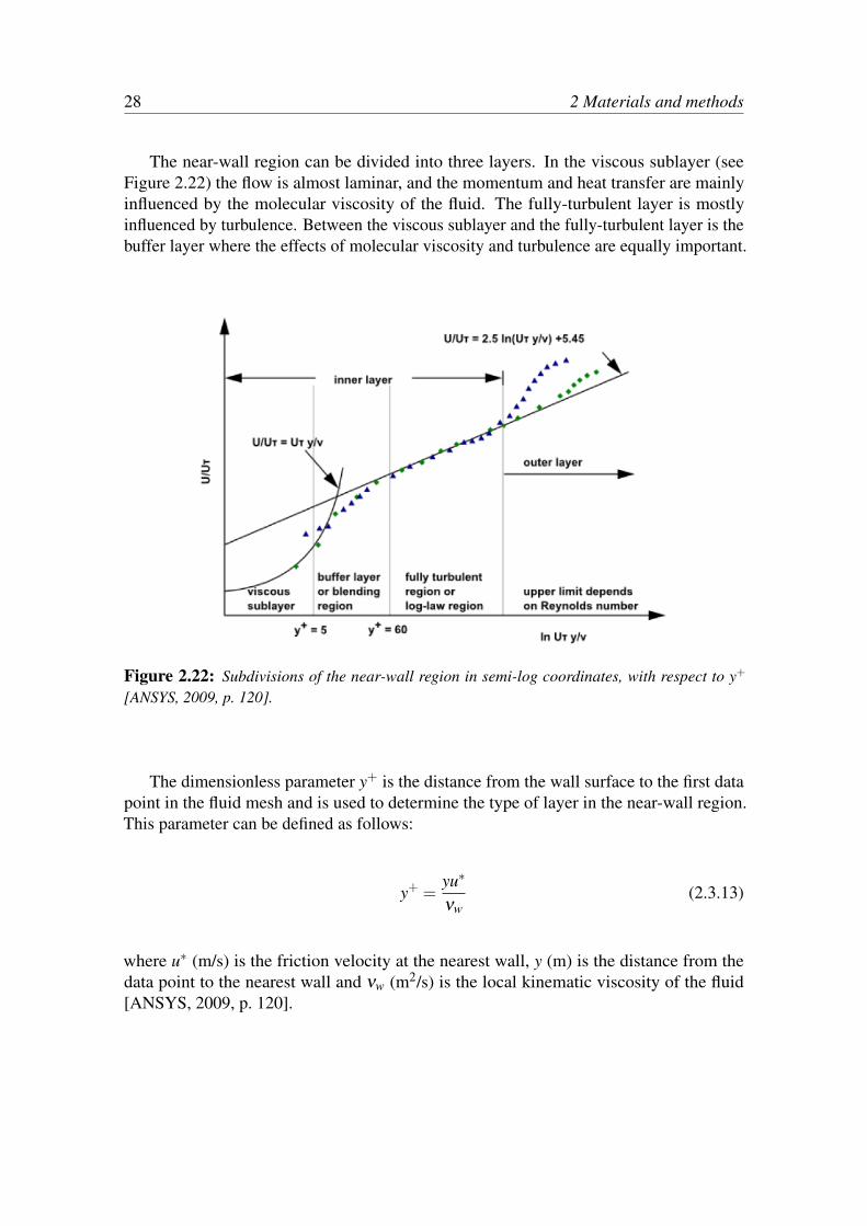
The near-wall region can be divided into three layers. In the viscous sublayer (seeFigure 2.22) the flow is almost laminar, and the momentum and heat transfer are mainlyinfluenced by the molecular viscosity of the fluid. The fully-turbulent layer is mostlyinfluenced by turbulence. Between the viscous sublayer and the fully-turbulent layer is thebuffer layer where the effects of molecular viscosity and turbulence are equally important.
Figure 2.22: Subdivisions of the near-wall region in semi-log coordinates, with respect to y+
[ANSYS, 2009, p. 120].
The dimensionless parameter y+ is the distance from the wall surface to the first datapoint in the fluid mesh and is used to determine the type of layer in the near-wall region.This parameter can be defined as follows:
y+ =yu∗
νw(2.3.13)
where u∗ (m/s) is the friction velocity at the nearest wall, y (m) is the distance from thedata point to the nearest wall and νw (m2/s) is the local kinematic viscosity of the fluid[ANSYS, 2009, p. 120].
2.3 Numerical modelling 29
2.3.9 Error estimationThe root mean square function is used to estimate the amount of deviation between theCFD- and measured results. The function is defined as:
RMS =
√√√√( 1N
N
∑i(TCFD−TEXP)
2
)(2.3.14)
where TCFD and TEXP are the calculated and experimental temperature values at eachmeasured point, respectively [Weisstein [2012]].

CHAPTER 3
Results and discussion
This chapter presents and compares the results from measurements and the CFD-models. Aturbulence model is selected for the air flow and the thermal contact resistance between fishand aluminium belt is determined. The selected turbulence model and the thermal contactresistance are then applied for different cases, involving longer periods of CBC-coolingincluding storage and a 3D case.
3.1 Experimental resultsMeasurements are conducted for four different tests where the temperature settings insidethe CBC-cooler is altered. The applied settings, presented in Table 3.1, are the idealsettings but the measured settings, which are used in the CFD model were obtained bymeasurements. The table also shows the chilling periods inside the CBC-cooler for eachtest. Test 4 consists twice of chilling periods of 15 and 30 minutes which is because themeasurements are made for fish with different masses. Test 1 and Test 3 with chillingperiods of 6 and 14 minutes, respectively, are used for comparison in this thesis. Theexperimental results which are not shown in this section are presented in Appendix A.
31
32 3 Results and discussion
Table 3.1: Applied temperature settings and chilling periods inside the CBC-cooler for the fourdifferent measurements.
Test no. 1 2 3 4
T∞ [◦C] -7.4 -13.0 -14.1 -13.6Chilling period [min] 6 10, 15, 20, 25 8, 14, 18 15, 30 ,15, 30, 0
Dimensions of the two fish specimen used for later comparison are presented in Table 3.2.The lengths L and L′ represent the total length and the length without head and tail as isshown in Figure 2.4.
Table 3.2: Dimensions of the fish specimen which are used for comparison for the two differenttemperature conditions in the CBC-cooler.
CBC settings L [cm] L′ [cm] m [kg]
Conventional 75 44 2.53Modified 72 40 2.77
3.1.1 Conventional CBC-cooler settings (Test 1)The settings used for the first case are the same as for conventional CBC-cooling of fishfillets, and are presented in Table 3.3.
Table 3.3: Conventional settings in the CBC-cooler along with the fish initial temperature.
u∞ [m/s] T∞ [◦C] T0 [◦C]
2.6 -7.4 4.3
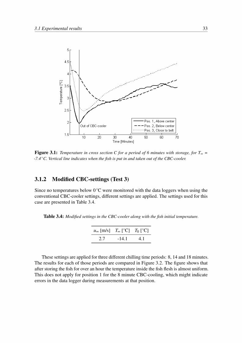
The fish is cooled for a period of 6 minutes in the CBC-cooler. The temperature profileinside the fish flesh during the CBC-cooling and a storage period of approximately 60minutes is presented in Figure 3.1. As shown in the figure, the fish is chilled down to atemperature close to 2◦C which is quite far from freezing. The ideal temperature for the fishafter CBC-cooling should be just below the initial freezing temperature of T f ,i=−0.91◦C,as discussed earlier. Thus the temperature settings and the cooling period are changed, asshown in Section 3.1.2.
It is clear, from Figure 3.1 (at t = 0 min), that the initial temperature of the fish flesh isnot uniform. The initial temperature, T0, in Table 3.3 is a selected value in the range of themeasured temperatures at the three positions.
3.1 Experimental results 33
Figure 3.1: Temperature in cross section C for a period of 6 minutes with storage, for T∞ =-7.4 ◦C. Vertical line indicates when the fish is put in and taken out of the CBC-cooler.
3.1.2 Modified CBC-settings (Test 3)
Since no temperatures below 0◦C were monitored with the data loggers when using theconventional CBC-cooler settings, different settings are applied. The settings used for thiscase are presented in Table 3.4.
Table 3.4: Modified settings in the CBC-cooler along with the fish initial temperature.
u∞ [m/s] T∞ [◦C] T0 [◦C]
2.7 -14.1 4.1
These settings are applied for three different chilling time periods: 8, 14 and 18 minutes.The results for each of those periods are compared in Figure 3.2. The figure shows thatafter storing the fish for over an hour the temperature inside the fish flesh is almost uniform.This does not apply for position 1 for the 8 minute CBC-cooling, which might indicateerrors in the data logger during measurements at that position.
34 3 Results and discussion
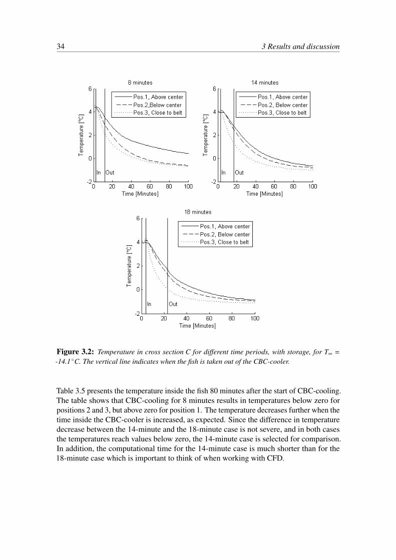
Figure 3.2: Temperature in cross section C for different time periods, with storage, for T∞ =-14.1 ◦C. The vertical line indicates when the fish is taken out of the CBC-cooler.
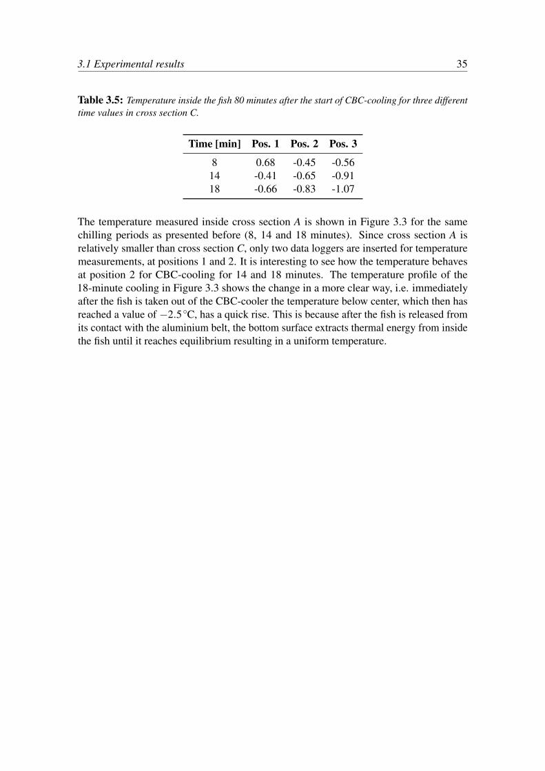
Table 3.5 presents the temperature inside the fish 80 minutes after the start of CBC-cooling.The table shows that CBC-cooling for 8 minutes results in temperatures below zero forpositions 2 and 3, but above zero for position 1. The temperature decreases further when thetime inside the CBC-cooler is increased, as expected. Since the difference in temperaturedecrease between the 14-minute and the 18-minute case is not severe, and in both casesthe temperatures reach values below zero, the 14-minute case is selected for comparison.In addition, the computational time for the 14-minute case is much shorter than for the18-minute case which is important to think of when working with CFD.
3.1 Experimental results 35
Table 3.5: Temperature inside the fish 80 minutes after the start of CBC-cooling for three differenttime values in cross section C.
Time [min] Pos. 1 Pos. 2 Pos. 3
8 0.68 -0.45 -0.5614 -0.41 -0.65 -0.9118 -0.66 -0.83 -1.07
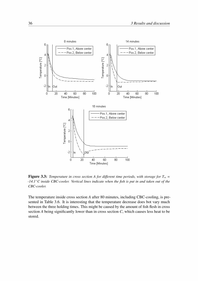
The temperature measured inside cross section A is shown in Figure 3.3 for the samechilling periods as presented before (8, 14 and 18 minutes). Since cross section A isrelatively smaller than cross section C, only two data loggers are inserted for temperaturemeasurements, at positions 1 and 2. It is interesting to see how the temperature behavesat position 2 for CBC-cooling for 14 and 18 minutes. The temperature profile of the18-minute cooling in Figure 3.3 shows the change in a more clear way, i.e. immediatelyafter the fish is taken out of the CBC-cooler the temperature below center, which then hasreached a value of −2.5◦C, has a quick rise. This is because after the fish is released fromits contact with the aluminium belt, the bottom surface extracts thermal energy from insidethe fish until it reaches equilibrium resulting in a uniform temperature.
36 3 Results and discussion
Figure 3.3: Temperature in cross section A for different time periods, with storage for T∞ =-14.1 ◦C inside CBC-cooler. Vertical lines indicate when the fish is put in and taken out of theCBC-cooler.
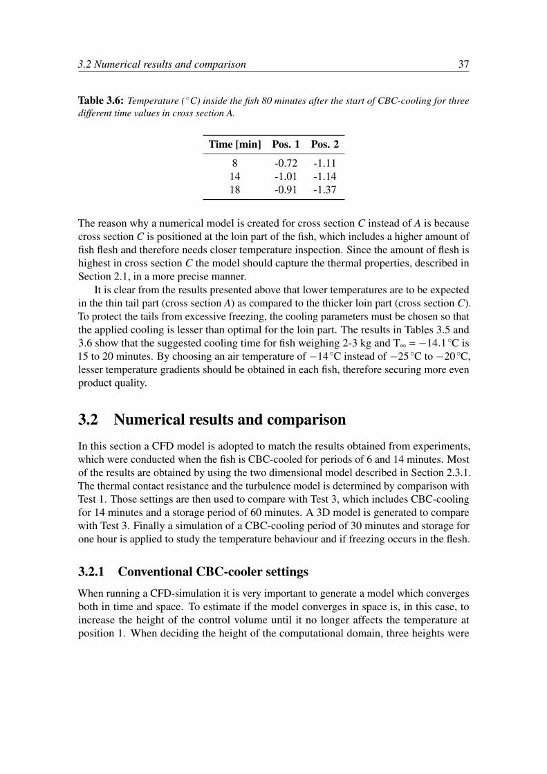
The temperature inside cross section A after 80 minutes, including CBC-cooling, is pre-sented in Table 3.6. It is interesting that the temperature decrease does bot vary muchbetween the three holding times. This might be caused by the amount of fish flesh in crosssection A being significantly lower than in cross section C, which causes less heat to bestored.
3.2 Numerical results and comparison 37
Table 3.6: Temperature ( ◦C) inside the fish 80 minutes after the start of CBC-cooling for threedifferent time values in cross section A.
Time [min] Pos. 1 Pos. 2
8 -0.72 -1.1114 -1.01 -1.1418 -0.91 -1.37
The reason why a numerical model is created for cross section C instead of A is becausecross section C is positioned at the loin part of the fish, which includes a higher amount offish flesh and therefore needs closer temperature inspection. Since the amount of flesh ishighest in cross section C the model should capture the thermal properties, described inSection 2.1, in a more precise manner.
It is clear from the results presented above that lower temperatures are to be expectedin the thin tail part (cross section A) as compared to the thicker loin part (cross section C).To protect the tails from excessive freezing, the cooling parameters must be chosen so thatthe applied cooling is lesser than optimal for the loin part. The results in Tables 3.5 and3.6 show that the suggested cooling time for fish weighing 2-3 kg and T∞ = −14.1◦C is15 to 20 minutes. By choosing an air temperature of −14◦C instead of −25◦C to −20◦C,lesser temperature gradients should be obtained in each fish, therefore securing more evenproduct quality.
3.2 Numerical results and comparisonIn this section a CFD model is adopted to match the results obtained from experiments,which were conducted when the fish is CBC-cooled for periods of 6 and 14 minutes. Mostof the results are obtained by using the two dimensional model described in Section 2.3.1.The thermal contact resistance and the turbulence model is determined by comparison withTest 1. Those settings are then used to compare with Test 3, which includes CBC-coolingfor 14 minutes and a storage period of 60 minutes. A 3D model is generated to comparewith Test 3. Finally a simulation of a CBC-cooling period of 30 minutes and storage forone hour is applied to study the temperature behaviour and if freezing occurs in the flesh.
3.2.1 Conventional CBC-cooler settingsWhen running a CFD-simulation it is very important to generate a model which convergesboth in time and space. To estimate if the model converges in space is, in this case, toincrease the height of the control volume until it no longer affects the temperature atposition 1. When deciding the height of the computational domain, three heights were
38 3 Results and discussion
tested: 150 mm, 200 mm and 250 mm. The results obtained with these different heightsshow that there is a difference in the solution between 150 mm and 200 mm but nodifference between 200 mm and 250 mm. The height of the computational domain istherefore set to 200 mm. Time convergence is obtained by adjusting the time step size sothat the Courant number (see Section 2.3.4) is satisfactory.
The settings in the CBC-cooler used for this comparison are as described in Section3.1.1. For these setting the temperature inside the fish does not reach a value below 2◦C, asshown in Section 3.1.1. As shown in Table 2.1 no significant changes occur with regardsto the thermal fish properties until below 0◦C.The measured temperature in the fish flesh isnot completely uniform and has an initial temperature ranging from 3.7◦C to 4.6◦C. Forthis comparison the initial temperature from FLUENT and measurements are given thesame value for the best comparison.
Thermal contact resistance
As mentioned in Section 2.2, three temperature data loggers, which were inserted in crosssection C two below center and one above (See Figure 2.5), are used for comparison.The thermal contact resistance, discussed in Section 2.3.7, is highly influential on thetemperature measured by the data loggers below center. Similarly the temperature abovethe center of the fish is mainly influenced with which turbulence model is used.
In research done by Margeirsson et al. [2011] a value of R = 0.050 m2 K/W was adoptedfor thermal contact resistance between fish fillets and food packaging. The value of R couldbe as high as 0.2 m2 K/W but since the water content of fresh cod is as high as 80−82%,a lower value of R may be expected. In this previosly mentioned research a value of R= 0.050 m2 K/W yielded a good agreement between experimental and simulated resultsand will therefore be examined in this study. The value of R for cod fish is a very delicateparameter which needs adjustment for different settings. Results obtained with valuesranging from R = 0.025 m2 K/W to R = 0.050 m2 K/W is introduced and compared withmeasurements.
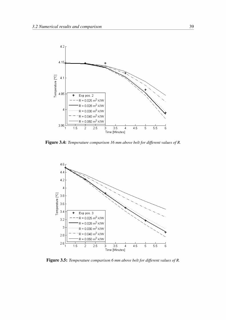
In this section the temperatures below the center of the fish are compared to decidewhat value of R is to be selected. Figures 3.4 and 3.5 give a visual comparison between theexperimental and calculated results for different values of R. A numerical comparison ispresented in Table 3.7 where the root mean square (RMS) error between measurementsand simulated results is compared for the different values of R. Note that the temperaturescales for Figures 3.4 and 3.5 range from 3.95 to 4.2◦C and 2.6 to 4.6◦C, respectively.
3.2 Numerical results and comparison 39
Figure 3.4: Temperature comparison 16 mm above belt for different values of R.
Figure 3.5: Temperature comparison 6 mm above belt for different values of R.
40 3 Results and discussion
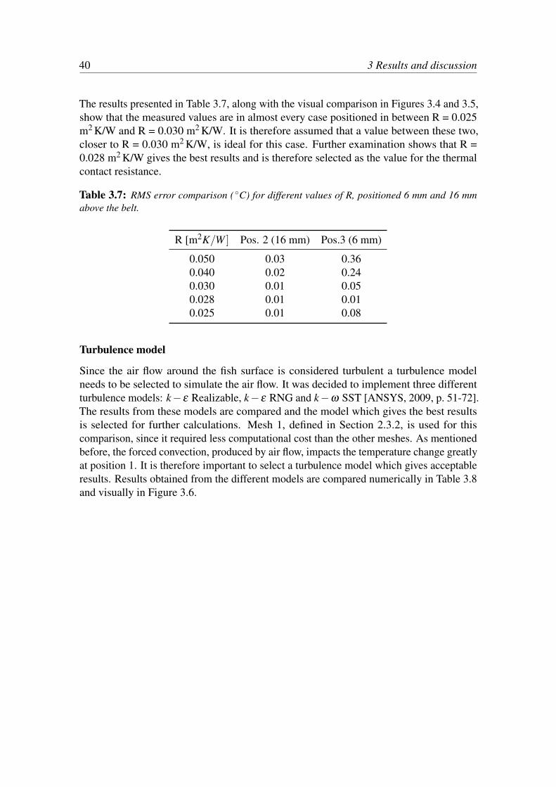
The results presented in Table 3.7, along with the visual comparison in Figures 3.4 and 3.5,show that the measured values are in almost every case positioned in between R = 0.025m2 K/W and R = 0.030 m2 K/W. It is therefore assumed that a value between these two,closer to R = 0.030 m2 K/W, is ideal for this case. Further examination shows that R =0.028 m2 K/W gives the best results and is therefore selected as the value for the thermalcontact resistance.
Table 3.7: RMS error comparison ( ◦C) for different values of R, positioned 6 mm and 16 mmabove the belt.
R [m2K/W ] Pos. 2 (16 mm) Pos.3 (6 mm)
0.050 0.03 0.360.040 0.02 0.240.030 0.01 0.050.028 0.01 0.010.025 0.01 0.08
Turbulence model
Since the air flow around the fish surface is considered turbulent a turbulence modelneeds to be selected to simulate the air flow. It was decided to implement three differentturbulence models: k−ε Realizable, k−ε RNG and k−ω SST [ANSYS, 2009, p. 51-72].The results from these models are compared and the model which gives the best resultsis selected for further calculations. Mesh 1, defined in Section 2.3.2, is used for thiscomparison, since it required less computational cost than the other meshes. As mentionedbefore, the forced convection, produced by air flow, impacts the temperature change greatlyat position 1. It is therefore important to select a turbulence model which gives acceptableresults. Results obtained from the different models are compared numerically in Table 3.8and visually in Figure 3.6.

3.2 Numerical results and comparison 41
Figure 3.6: Temperature comparison 56 mm above belt for different turbulence models
The results presented in Figure 3.6 and Table 3.8 show that the k− ε RNG turbulencemodel gives the best comparison. The k− ε RNG turbulence model is therefore used forfurther calculations.
Table 3.8: RMS error comparison ( ◦C) for different turbulence models positioned 56 mm abovebelt.
Turbulence model Pos. 1 (56 mm)k-ε Realizable 0.18k-ε RNG 0.14k-ω SST 0.25
3.2.2 Mesh refinement
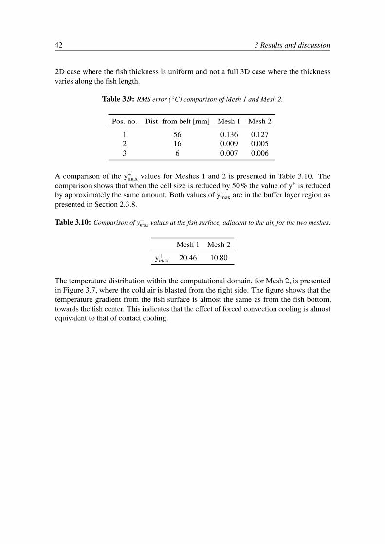
The selected R-value and turbulence model are now applied to Mesh 2, to see if it yieldsmore accurate results. The results for the two meshes are compared in Table 3.9. Thehighest percentage difference is approximately 44% at position 2 (16 mm above belt).Since this is only an increase from a RMS error of 0.009◦C to 0.005◦C, which is verysmall, no further mesh refinement is applied for this case. The highest RMS error, atposition 1 (45 mm above belt), might be explained by the fact that these results are for a
42 3 Results and discussion
2D case where the fish thickness is uniform and not a full 3D case where the thicknessvaries along the fish length.
Table 3.9: RMS error ( ◦C) comparison of Mesh 1 and Mesh 2.
Pos. no. Dist. from belt [mm] Mesh 1 Mesh 2
1 56 0.136 0.1272 16 0.009 0.0053 6 0.007 0.006
A comparison of the y+max values for Meshes 1 and 2 is presented in Table 3.10. The
comparison shows that when the cell size is reduced by 50% the value of y+ is reducedby approximately the same amount. Both values of y+
max are in the buffer layer region aspresented in Section 2.3.8.
Table 3.10: Comparison of y+max values at the fish surface, adjacent to the air, for the two meshes.
Mesh 1 Mesh 2
y+max 20.46 10.80
The temperature distribution within the computational domain, for Mesh 2, is presentedin Figure 3.7, where the cold air is blasted from the right side. The figure shows that thetemperature gradient from the fish surface is almost the same as from the fish bottom,towards the fish center. This indicates that the effect of forced convection cooling is almostequivalent to that of contact cooling.
3.2 Numerical results and comparison 43
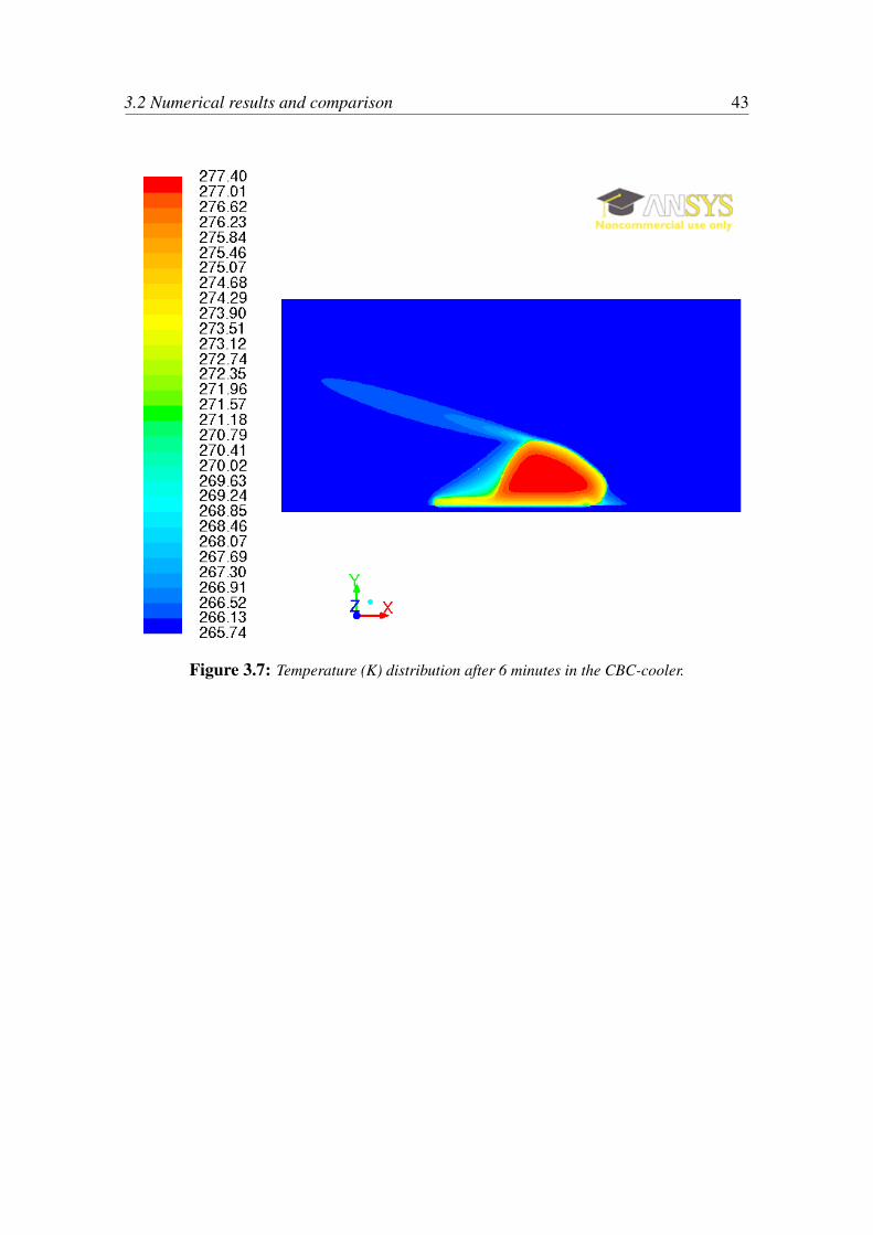
Figure 3.7: Temperature (K) distribution after 6 minutes in the CBC-cooler.
44 3 Results and discussion
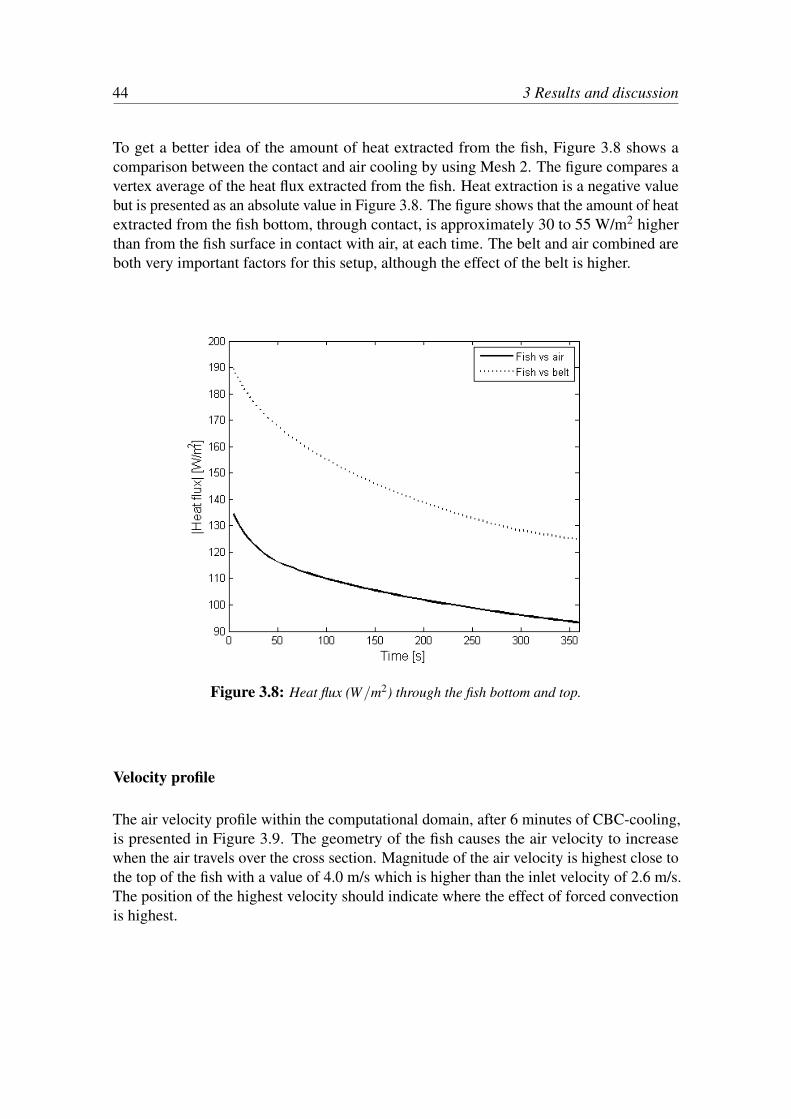
To get a better idea of the amount of heat extracted from the fish, Figure 3.8 shows acomparison between the contact and air cooling by using Mesh 2. The figure compares avertex average of the heat flux extracted from the fish. Heat extraction is a negative valuebut is presented as an absolute value in Figure 3.8. The figure shows that the amount of heatextracted from the fish bottom, through contact, is approximately 30 to 55 W/m2 higherthan from the fish surface in contact with air, at each time. The belt and air combined areboth very important factors for this setup, although the effect of the belt is higher.
Figure 3.8: Heat flux (W/m2) through the fish bottom and top.
Velocity profile
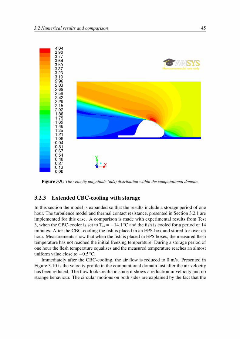
The air velocity profile within the computational domain, after 6 minutes of CBC-cooling,is presented in Figure 3.9. The geometry of the fish causes the air velocity to increasewhen the air travels over the cross section. Magnitude of the air velocity is highest close tothe top of the fish with a value of 4.0 m/s which is higher than the inlet velocity of 2.6 m/s.The position of the highest velocity should indicate where the effect of forced convectionis highest.
3.2 Numerical results and comparison 45
Figure 3.9: The velocity magnitude (m/s) distribution within the computational domain.
3.2.3 Extended CBC-cooling with storageIn this section the model is expanded so that the results include a storage period of onehour. The turbulence model and thermal contact resistance, presented in Section 3.2.1 areimplemented for this case. A comparison is made with experimental results from Test3, when the CBC-cooler is set to T∞ = −14.1◦C and the fish is cooled for a period of 14minutes. After the CBC-cooling the fish is placed in an EPS-box and stored for over anhour. Measurements show that when the fish is placed in EPS boxes, the measured fleshtemperature has not reached the initial freezing temperature. During a storage period ofone hour the flesh temperature equalises and the measured temperature reaches an almostuniform value close to −0.5◦C.
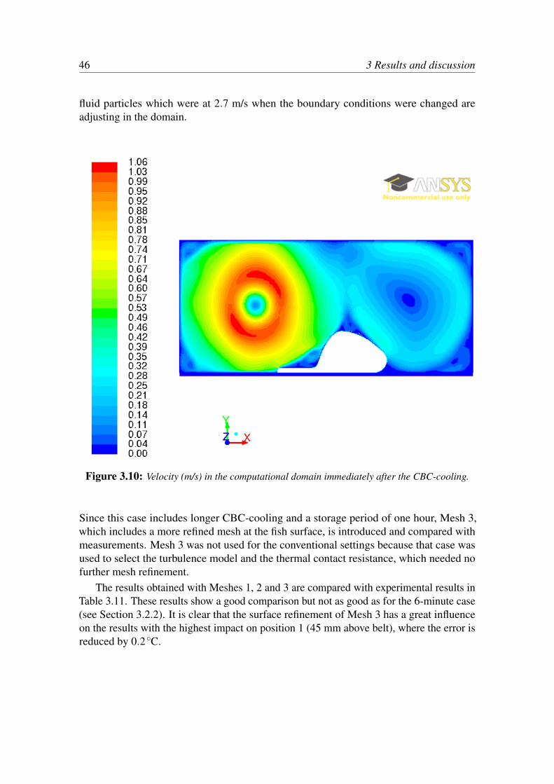
Immediately after the CBC-cooling, the air flow is reduced to 0 m/s. Presented inFigure 3.10 is the velocity profile in the computational domain just after the air velocityhas been reduced. The flow looks realistic since it shows a reduction in velocity and nostrange behaviour. The circular motions on both sides are explained by the fact that the
46 3 Results and discussion
fluid particles which were at 2.7 m/s when the boundary conditions were changed areadjusting in the domain.
Figure 3.10: Velocity (m/s) in the computational domain immediately after the CBC-cooling.
Since this case includes longer CBC-cooling and a storage period of one hour, Mesh 3,which includes a more refined mesh at the fish surface, is introduced and compared withmeasurements. Mesh 3 was not used for the conventional settings because that case wasused to select the turbulence model and the thermal contact resistance, which needed nofurther mesh refinement.
The results obtained with Meshes 1, 2 and 3 are compared with experimental results inTable 3.11. These results show a good comparison but not as good as for the 6-minute case(see Section 3.2.2). It is clear that the surface refinement of Mesh 3 has a great influenceon the results with the highest impact on position 1 (45 mm above belt), where the error isreduced by 0.2◦C.
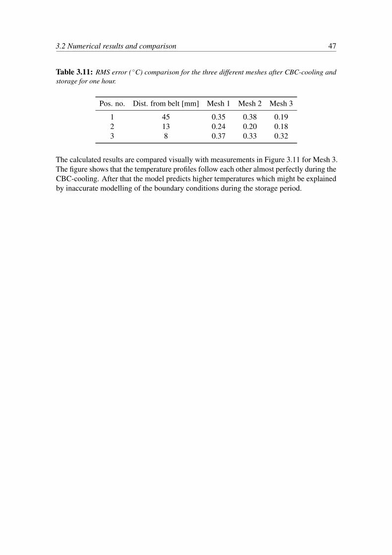
3.2 Numerical results and comparison 47
Table 3.11: RMS error ( ◦C) comparison for the three different meshes after CBC-cooling andstorage for one hour.
Pos. no. Dist. from belt [mm] Mesh 1 Mesh 2 Mesh 3
1 45 0.35 0.38 0.192 13 0.24 0.20 0.183 8 0.37 0.33 0.32
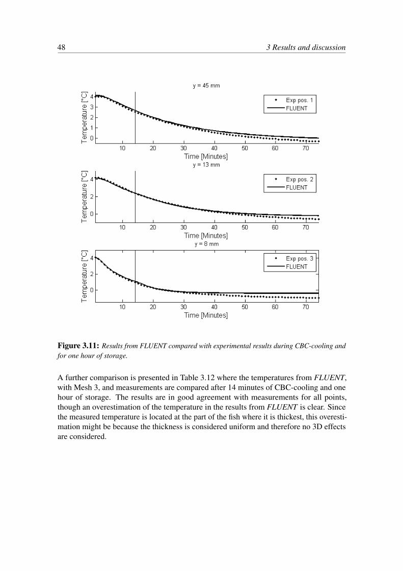
The calculated results are compared visually with measurements in Figure 3.11 for Mesh 3.The figure shows that the temperature profiles follow each other almost perfectly during theCBC-cooling. After that the model predicts higher temperatures which might be explainedby inaccurate modelling of the boundary conditions during the storage period.
48 3 Results and discussion
Figure 3.11: Results from FLUENT compared with experimental results during CBC-cooling andfor one hour of storage.
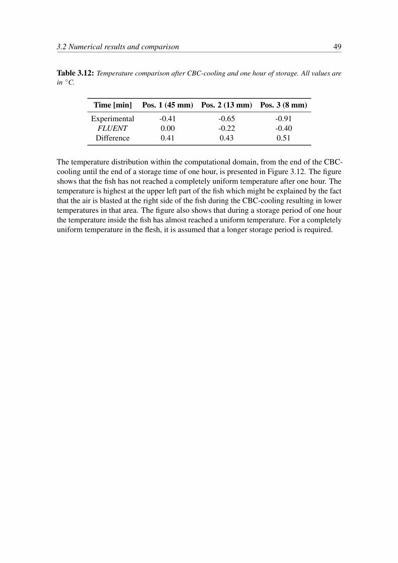
A further comparison is presented in Table 3.12 where the temperatures from FLUENT,with Mesh 3, and measurements are compared after 14 minutes of CBC-cooling and onehour of storage. The results are in good agreement with measurements for all points,though an overestimation of the temperature in the results from FLUENT is clear. Sincethe measured temperature is located at the part of the fish where it is thickest, this overesti-mation might be because the thickness is considered uniform and therefore no 3D effectsare considered.
3.2 Numerical results and comparison 49
Table 3.12: Temperature comparison after CBC-cooling and one hour of storage. All values arein ◦C.
Time [min] Pos. 1 (45 mm) Pos. 2 (13 mm) Pos. 3 (8 mm)
Experimental -0.41 -0.65 -0.91FLUENT 0.00 -0.22 -0.40Difference 0.41 0.43 0.51
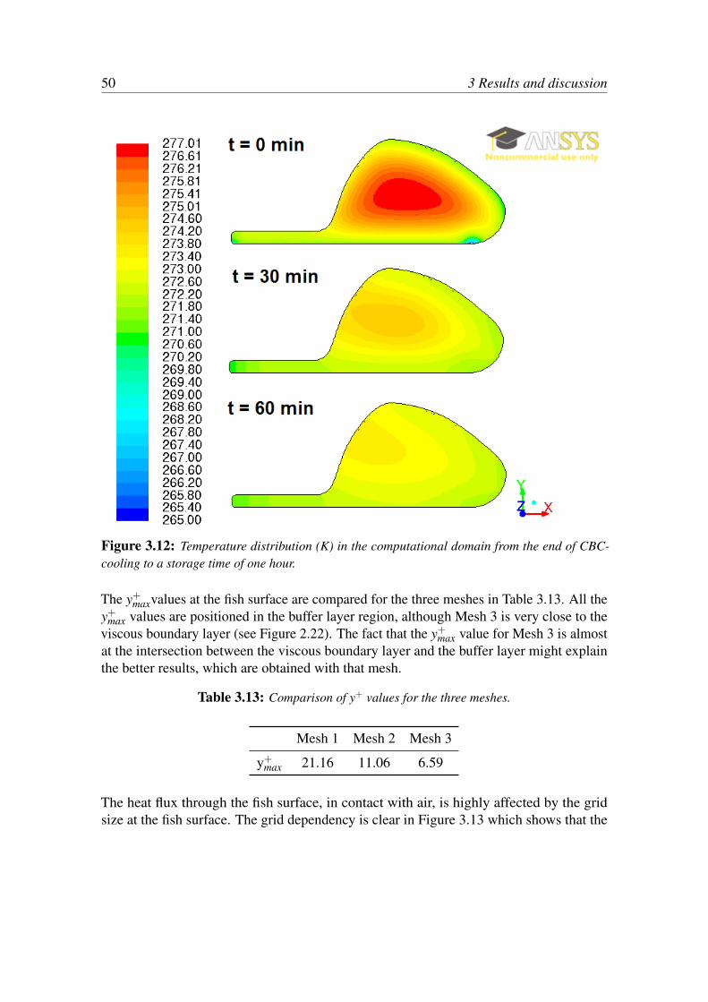
The temperature distribution within the computational domain, from the end of the CBC-cooling until the end of a storage time of one hour, is presented in Figure 3.12. The figureshows that the fish has not reached a completely uniform temperature after one hour. Thetemperature is highest at the upper left part of the fish which might be explained by the factthat the air is blasted at the right side of the fish during the CBC-cooling resulting in lowertemperatures in that area. The figure also shows that during a storage period of one hourthe temperature inside the fish has almost reached a uniform temperature. For a completelyuniform temperature in the flesh, it is assumed that a longer storage period is required.
50 3 Results and discussion
Figure 3.12: Temperature distribution (K) in the computational domain from the end of CBC-cooling to a storage time of one hour.
The y+maxvalues at the fish surface are compared for the three meshes in Table 3.13. All they+max values are positioned in the buffer layer region, although Mesh 3 is very close to theviscous boundary layer (see Figure 2.22). The fact that the y+max value for Mesh 3 is almostat the intersection between the viscous boundary layer and the buffer layer might explainthe better results, which are obtained with that mesh.
Table 3.13: Comparison of y+ values for the three meshes.
Mesh 1 Mesh 2 Mesh 3
y+max 21.16 11.06 6.59
The heat flux through the fish surface, in contact with air, is highly affected by the gridsize at the fish surface. The grid dependency is clear in Figure 3.13 which shows that the
3.2 Numerical results and comparison 51
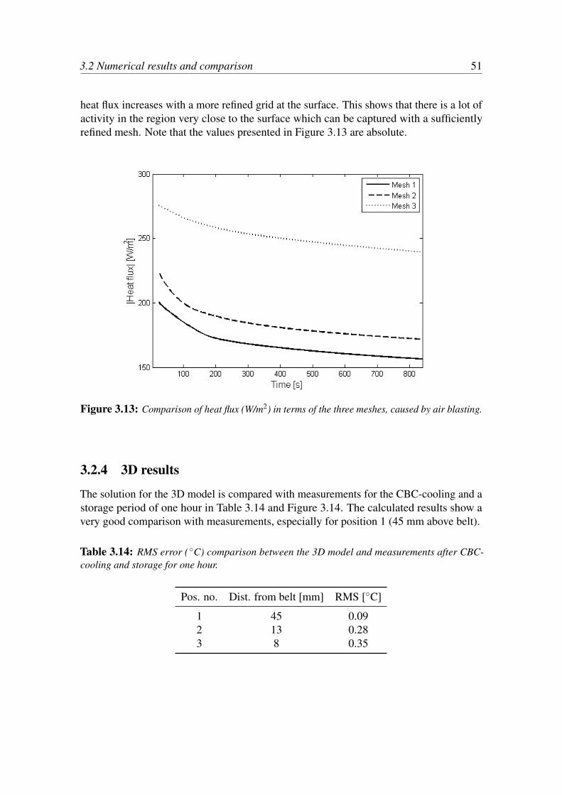
heat flux increases with a more refined grid at the surface. This shows that there is a lot ofactivity in the region very close to the surface which can be captured with a sufficientlyrefined mesh. Note that the values presented in Figure 3.13 are absolute.
Figure 3.13: Comparison of heat flux (W/m2) in terms of the three meshes, caused by air blasting.
3.2.4 3D results
The solution for the 3D model is compared with measurements for the CBC-cooling and astorage period of one hour in Table 3.14 and Figure 3.14. The calculated results show avery good comparison with measurements, especially for position 1 (45 mm above belt).
Table 3.14: RMS error ( ◦C) comparison between the 3D model and measurements after CBC-cooling and storage for one hour.
Pos. no. Dist. from belt [mm] RMS [◦C]
1 45 0.092 13 0.283 8 0.35
52 3 Results and discussion
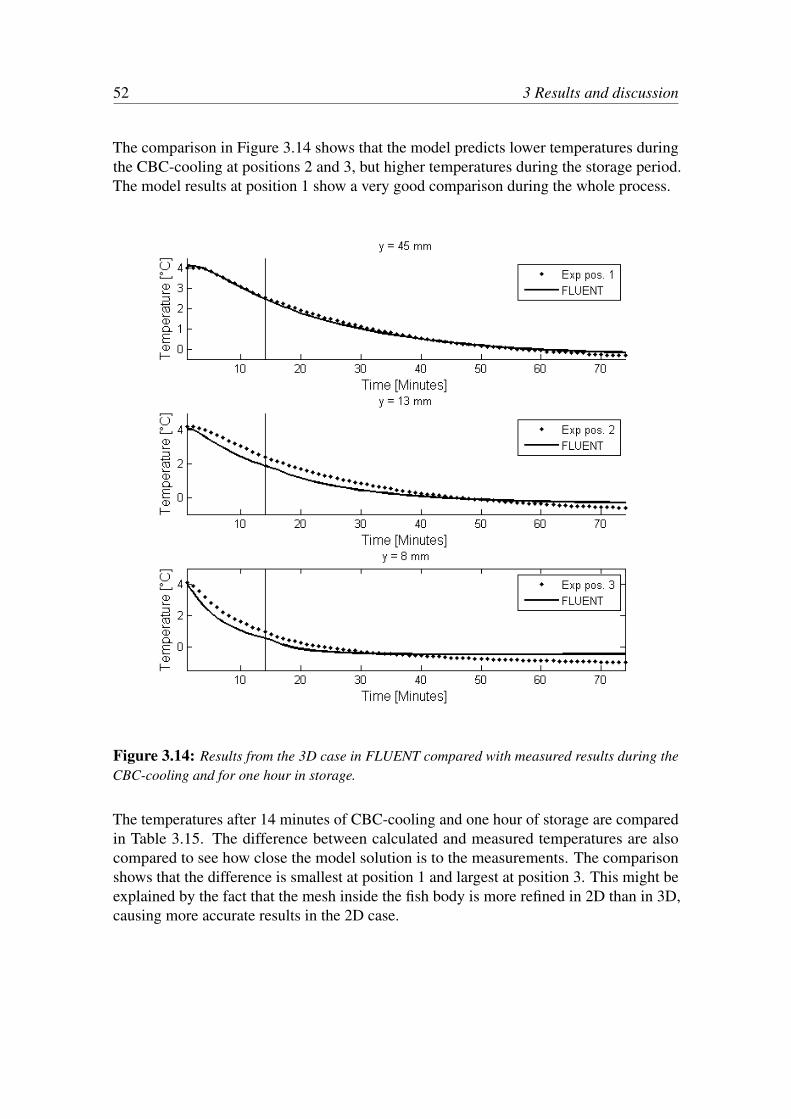
The comparison in Figure 3.14 shows that the model predicts lower temperatures duringthe CBC-cooling at positions 2 and 3, but higher temperatures during the storage period.The model results at position 1 show a very good comparison during the whole process.
Figure 3.14: Results from the 3D case in FLUENT compared with measured results during theCBC-cooling and for one hour in storage.
The temperatures after 14 minutes of CBC-cooling and one hour of storage are comparedin Table 3.15. The difference between calculated and measured temperatures are alsocompared to see how close the model solution is to the measurements. The comparisonshows that the difference is smallest at position 1 and largest at position 3. This might beexplained by the fact that the mesh inside the fish body is more refined in 2D than in 3D,causing more accurate results in the 2D case.

3.2 Numerical results and comparison 53
Table 3.15: Temperature comparison ( ◦C) after CBC-cooling and one hour of storage.
Time [min] Pos. 1 Pos. 2 Pos. 3
Experimental -0.41 -0.65 -0.91FLUENT -0.13 -0.27 -0.42Difference 0.28 0.38 0.49
A longitudinal cross section of the fish, positioned at the same x-coordinates as thetemperature monitors (See Figures 2.5 and 2.11), is examined. The temperature distributionalong the fish length, with a 10 min interval, during the storage period is shown in Figure3.15. The vertical lines in the figure show the position of cross section C. The figure showsthat the fish flesh keeps getting colder without any applied external cooling, such as airblasting. It is clear that the colder parts of the fish, closer to the tail, affect the temperatureat cross section C by removing more heat from it than if the fish thickness is uniform. Ifthe thickness of the fish is uniform, as for the 2D case, the longitudinal effect would lookthe same as at the left hand side of Figure 3.15, i.e. the effect would be negligible.
Figure 3.15: Temperature distribution (K) in the length cross section of the fish during storage.
The y+max value at the fish surface, obtained from the CFD model, is 12.90. This value is

54 3 Results and discussion
positioned in the buffer layer region (see Figure 2.22) and has almost the same value asMesh 2. More accurate results might be obtained by refining the grid at the fish surface,resulting in a value of y+max closer to the viscous sublayer, which was obtained with Mesh3.
3.2.5 30 minute CBC-coolingIn this section a 30 minute long CBC-cooling process is simulated. Since no measurementswere made to compare with these results, the results are only used to see what the modelpredicts and how it handles the fish thermal property changes as described in section 2.1.The temperature is monitored at the same positions as for Test 3 (see Section 3.2.3), i.e. 8,13 and 45 mm above belt.
The predicted temperature in the fish flesh at cross section C is presented in Figure3.16. The lowest value at position 3 is T = −0.78◦C which shows that the fish flesh hasnot reached the initial freezing temperature of T f ,i = −0.91◦C.
Figure 3.16: Results from the CFD model in FLUENT where 30 minutes of CBC-cooling and onehour of storage are applied.
The temperature distribution within the cross section after one hour of storage, which is
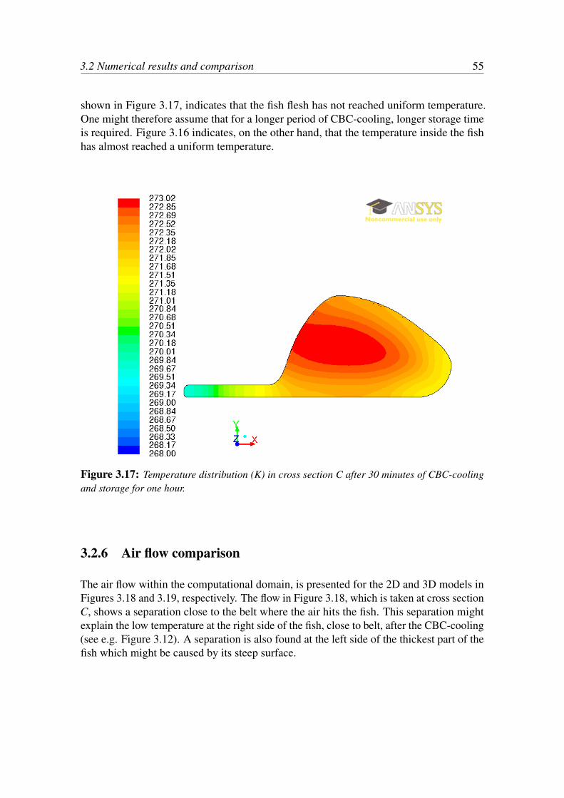
3.2 Numerical results and comparison 55
shown in Figure 3.17, indicates that the fish flesh has not reached uniform temperature.One might therefore assume that for a longer period of CBC-cooling, longer storage timeis required. Figure 3.16 indicates, on the other hand, that the temperature inside the fishhas almost reached a uniform temperature.
Figure 3.17: Temperature distribution (K) in cross section C after 30 minutes of CBC-coolingand storage for one hour.
3.2.6 Air flow comparison
The air flow within the computational domain, is presented for the 2D and 3D models inFigures 3.18 and 3.19, respectively. The flow in Figure 3.18, which is taken at cross sectionC, shows a separation close to the belt where the air hits the fish. This separation mightexplain the low temperature at the right side of the fish, close to belt, after the CBC-cooling(see e.g. Figure 3.12). A separation is also found at the left side of the thickest part of thefish which might be caused by its steep surface.

56 3 Results and discussion
Figure 3.18: Air flow at cross section C in 2D.
The flow presented in Figure 3.19 is from the 3D model and is positioned at the end of thefish, closest to the head. The fish geometry is smoother at this position, hence causing lessseparation in the air flow than what is shown in Figure 3.18. Both figures have in commonthe large separation which starts to form after the air has hit the fish. If the computationaldomain is larger, positioning the air outlet further to the left, different behaviour of the airflow might be observed. Since this large separation is located behind the fish it is assumedthat its effects are negligible to the final results.
Figure 3.19: Air flow close to the fish head in 3D.
3.2 Numerical results and comparison 57
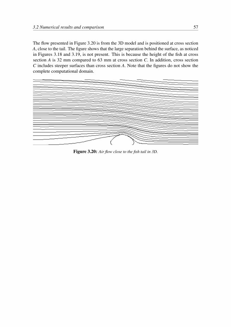
The flow presented in Figure 3.20 is from the 3D model and is positioned at cross sectionA, close to the tail. The figure shows that the large separation behind the surface, as noticedin Figures 3.18 and 3.19, is not present. This is because the height of the fish at crosssection A is 32 mm compared to 63 mm at cross section C. In addition, cross sectionC includes steeper surfaces than cross section A. Note that the figures do not show thecomplete computational domain.
Figure 3.20: Air flow close to the fish tail in 3D.

CHAPTER 4
Conclusions
Results from the CFD simulations were generally in good agreement with the experimentalresults. The thermal contact resistance between the fish and aluminium belt was determinedas R = 0.028 m2 K/W in Section 3.2.1. For the conventional CBC-cooler settings, this Rvalue resulted in RMS errors of 0.009◦C and 0.007◦C at positions 2 and 3, respectively.Note that this comparison only included a chilling period of 6 minutes and no storage.The same R value was applied for the extended chilling process, including storage, inSection 3.2.3. For that process, RMS errors of 0.183◦C and 0.319◦C were obtained at thecorresponding positions. This high increase in the error might be caused by the storageperiod, which was included for the second case, or that the thermal contact resistance Rchanges between fish samples.
The k− ε RNG turbulence model was preferred over the k− ε Realisable and k−ω
SST models to simulate the air flow in the computational domain. The model was appliedfor three different meshes for the extended chilling period with storage. Mesh 3, whichincluded a refined grid at the fish surface adjacent to the air, yielded the best results.
A simulation of the 3D model showed that the height differences along the fish effectedthe temperature distribution at cross section C. The results from the best 2D case (Mesh 3)and the 3D case are compared in Table 4.1. It is clear that the 2D and 3D results are not invery good agreement when compared to each other. The 3D model gives very good resultsfor position 1 but not as good as the 2D model for positions 2 and 3. The most likelyreason for this difference is, as mentioned before, the longitudinal effect of the model, i.e.the height difference along the fish length. The contact area between the fish and belt/EPSbox also varies along the fish length (see Figure 2.15), which might cause this difference.
59
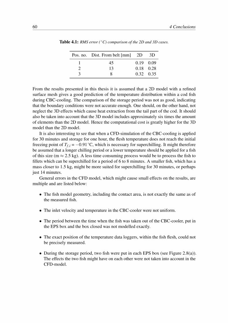
60 4 Conclusions
Table 4.1: RMS error ( ◦C) comparison of the 2D and 3D cases.
Pos. no. Dist. From belt [mm] 2D 3D
1 45 0.19 0.092 13 0.18 0.283 8 0.32 0.35
From the results presented in this thesis it is assumed that a 2D model with a refinedsurface mesh gives a good prediction of the temperature distribution within a cod fishduring CBC-cooling. The comparison of the storage period was not as good, indicatingthat the boundary conditions were not accurate enough. One should, on the other hand, notneglect the 3D effects which cause heat extraction from the tail part of the cod. It shouldalso be taken into account that the 3D model includes approximately six times the amountof elements than the 2D model. Hence the computational cost is greatly higher for the 3Dmodel than the 2D model.
It is also interesting to see that when a CFD-simulation of the CBC-cooling is appliedfor 30 minutes and storage for one hour, the flesh temperature does not reach the initialfreezing point of Tf ,i = −0.91◦C, which is necessary for superchilling. It might thereforebe assumed that a longer chilling period or a lower temperature should be applied for a fishof this size (m ≈ 2.5 kg). A less time consuming process would be to process the fish tofillets which can be superchilled for a period of 6 to 8 minutes. A smaller fish, which has amass closer to 1.5 kg, might be more suited for superchilling for 30 minutes, or perhapsjust 14 minutes.
General errors in the CFD model, which might cause small effects on the results, aremultiple and are listed below:
• The fish model geometry, including the contact area, is not exactly the same as ofthe measured fish.
• The inlet velocity and temperature in the CBC-cooler were not uniform.
• The period between the time when the fish was taken out of the CBC-cooler, put inthe EPS box and the box closed was not modelled exactly.
• The exact position of the temperature data loggers, within the fish flesh, could notbe precisely measured.
• During the storage period, two fish were put in each EPS box (see Figure 2.8(a)).The effects the two fish might have on each other were not taken into account in theCFD-model.
4 61
The results obtained in this study show that CFD modelling in terms of fluid flow andheat transfer has proven to be a realistic and functional tool to simulate superchilling ofwhole fish in a CBC-cooler. In future work CFD-modelling can be used to determineoptimal values for parameters such as holding time, chilling temperature and air velocity.

Bibliography
ANSYS. Ansys fluent 12.0 theory guide, 2009.
M. G. Arnþórsdóttir, S. Arason, and B. Margeirsson. Combined blast and contact cooling:Effects on physiochemical characteristics of fresh haddock (melanogrammus aeglefinus)fillets. (Matís report 14-08), 2008.
K. A. Fikiin. Ice content prediction methods during food freezing: a survey of the easterneuropean literature. Journal of Food Engineering, 1998.
H. Gao. Methods of pre-cooling for fresh cod (gadus morhua) and influences on qualityduring chilled storage at −1.5◦C. Technical report, The United Nations University:Fisheries Training Programme, 2007.
E. Granryd. Refrigerating Engineering - Part II. Royal Institute of Technology, KTH,Stockholm, 2005.
J. Holman. Heat Transfer. McGraw Hill, New York, 10 edition, 2010.
M. iButton R© Devices. ibutton products: ibuttons. http://www.maxim-ic.com/products/ibutton/products/ibuttons.cfm, 2011. Accessed August 10th,2011.
E. Instruments. 451126 - cfm/cmm vane anemometer datalogger. http://www.extech.com/instruments/categories.asp?catid=1, 2011. AccessedAugust 10th, 2011.
W. A. Johnston, A. R. Nicholson, and G. D. Stroud. Freezing and refrigerated storage infisheries, 1994. Accessed February 15th, 2012.
63
64 Bibliography
H. L. Lauzon, B. Margeirsson, K. Sveinsdóttir, M. Guðjónsdóttir, M. G. Karlsdóttir, andE. Martinsdóttir. Overview on fish quality research. impact of fish handling, processing,storage and logistics on fish quality deterioration. Matís report, (39-10), 2010.
J. H. Lienhard IV and J. H. Lienhard V. A Heat Transfer Textbook. Phlogiston Press,Cambridge Massachusets, fourth edition, 2010.
H. Magnússon, H. L. Lauzon, K. Sveinsdóttir, B. Margeirsson, E. Reynisson, A. R.Rúnarsson, M. Guðjónsdóttir, K. A. Þórarinsdóttir, S. Arason, and E. Martinsdóttir. Theeffect of different cooling techniques and temperature fluctuations on the storage life ofcod fillets (gadus morhua). Matís report, (23-09), 2009.
B. Margeirsson, H. L. Lauzon, L. Þorvaldsson, S. V. Árnason, S. Arason, K. L. Valtýsdóttir,and E. Martinsdóttir. Optimised chilling protocols for fresh fish. Matís report, (54-10),2010.
B. Margeirsson, H. Pálsson, V. Popov, R. Gospavic, S. Arason, K. Sveinsdóttir, andM. Þór Jónsson. Numerical modelling of temperature fluctuations in superchilled fishloins packaged in expanded polystyrene and stored at dynamic temperature conditions.International Journal of Refrigeration, 2012.
B. Margeirsson, R. Gospavic, H. Pálsson, S. Arason, and V. Popov. Experimental andnumerical modelling comparison of thermal performance of expanded polystyrene andcorrugated plastic packaging for fresh fish. 34(2):573–585, 2011.
E. Martinsdóttir, K. Sveinsdóttir, J. Luten, R. Schelvis-Smit, and G. Hyldig. Referencemanual for the fish sector : Sensory evaluation of fish freshness. QIM Eurofish, 2001.
E. Martinsdóttir, B. Guðbjörnsdóttir, and H. L. Lauzon. Áhrif roðkælingar á gæði fiskflaka.(Icelandic Fisheries Laboratories-report 03-04), 2004.
E. Martinsdóttir, B. Guðbjörnsdóttir, and H. L. Lauzon. Áhrif roðkælingar á gæði fiskflaka:Map-pökkuð og þídd. (Icelandic Fisheries Laboratories-report 10-05), 2005.
E. Martinsdóttir, H. L. Lauzon, B. Margeirsson, K. Sveinsdóttir, L. Þorvaldsson, H. Mag-nússon, E. Reynisson, A. V. Jónsdóttir, S. Arason, and M. Eden. The effect of coolingmethods at processing and use of gel-packs on storage life of cod (gadus morhua) loins -effect of transport via air and sea on temperature control and retail-packaging on coddeterioration. Matís report, (18-10), 2010.
G. Olafsdóttir, H. L. Lauzon, E. Martinsdóttir, J. Oehlenschläger, and K. Kristbergsson.Evaluation of shelf life of superchilled cod (gadus morhua) fillets and the influence oftemperature fluctuations during storage on microbial and chemical quality indicators.2006.
Bibliography 65
S. Rahman. Food properties handbook. CRC Press/Taylor Francis Group, 2009.
C. Rha. Theory, Determination and Control of Physical Properties of Food Materials.Reidel Publishing, Dordrecht, Boston, 1975.
K. L. Valtýsdóttir, B. Margeirsson, S. Arason, H. L. Lauzon, and E. Martinsdóttir. Guide-lines for precooling of fresh fish during processing and choice of packaging with respectto temperature control in cold chains. Matís report, (40-10), 2010.
E. W. Weisstein. Root mean square @ONLINE, 2012.
F. M. White. Viscous Fluid Flow. McGraw - Hill, third edition, 2006.
J. Zueco, F. Alhama, and C. G. Fernandez. Inverse determination of the specific heat offoods. Journal of Food Engineering, 64(3), 2004.

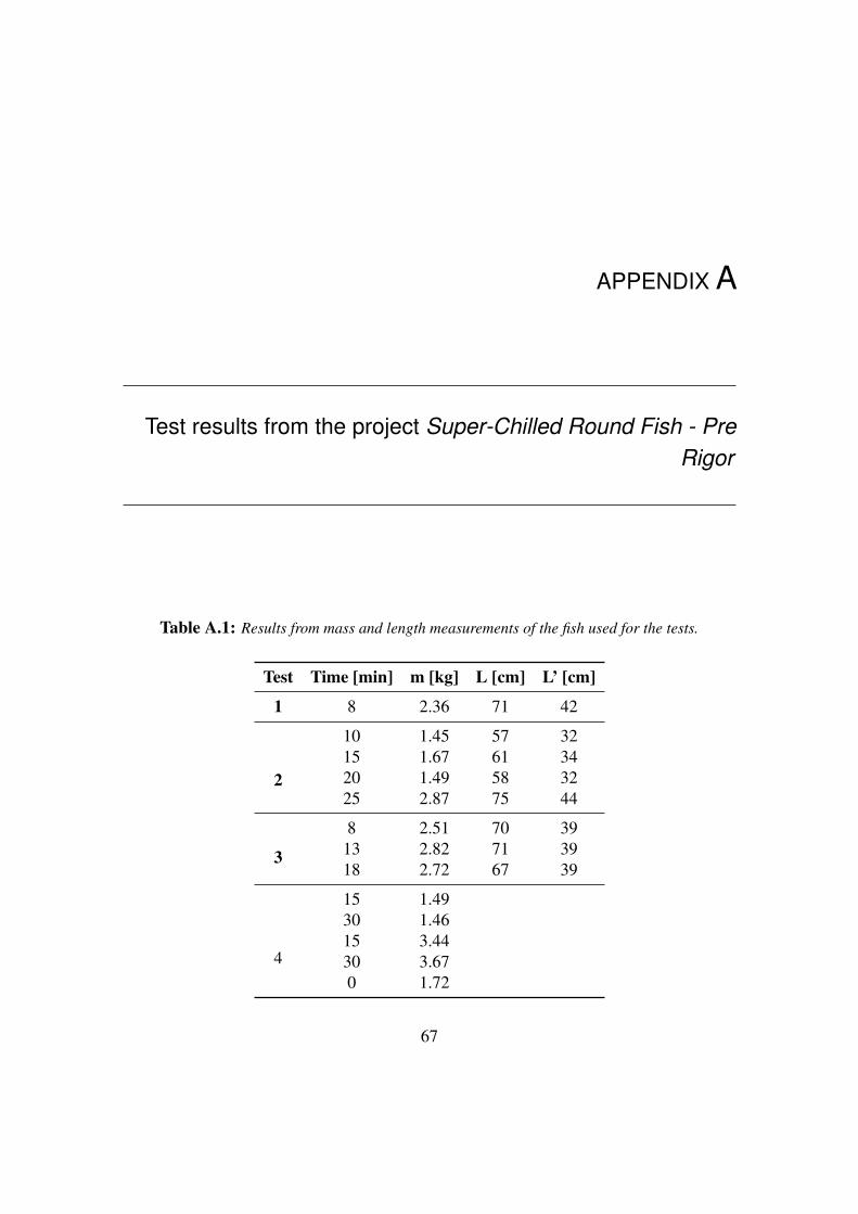
APPENDIX A
Test results from the project Super-Chilled Round Fish - PreRigor
Table A.1: Results from mass and length measurements of the fish used for the tests.
Test Time [min] m [kg] L [cm] L’ [cm]
1 8 2.36 71 42
2
10 1.45 57 3215 1.67 61 3420 1.49 58 3225 2.87 75 44
3
8 2.51 70 3913 2.82 71 3918 2.72 67 39
4
15 1.4930 1.4615 3.4430 3.670 1.72
67
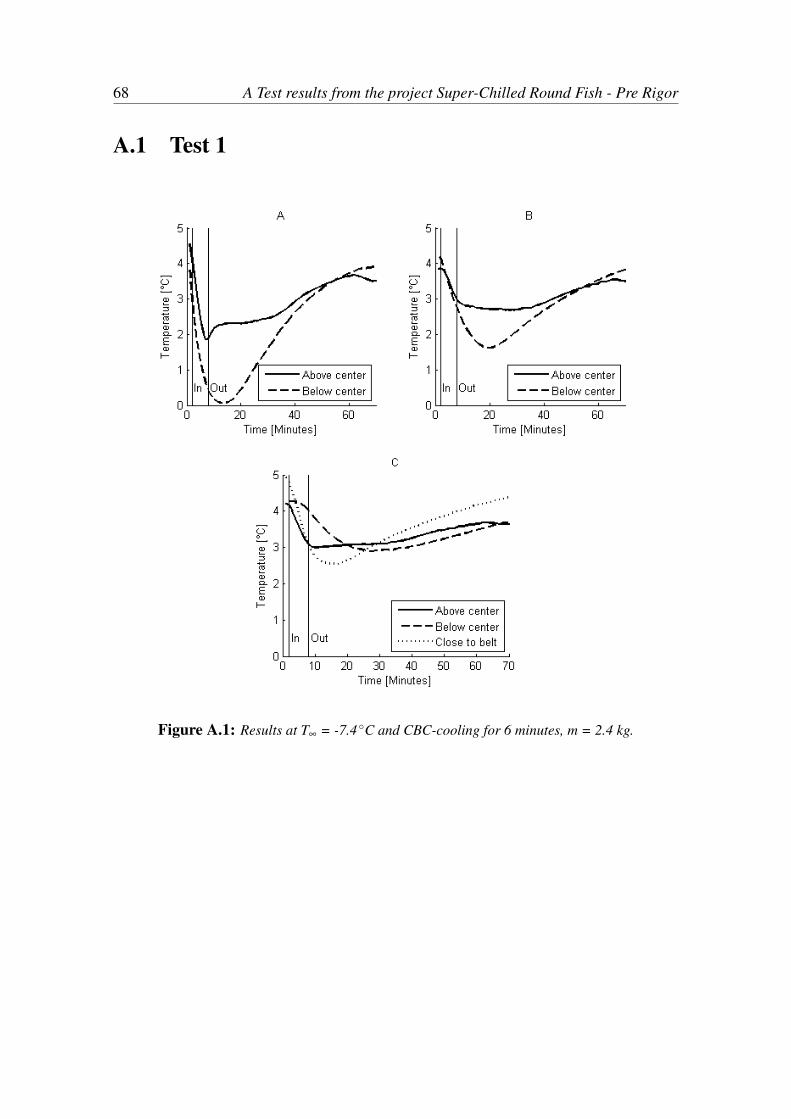
68 A Test results from the project Super-Chilled Round Fish - Pre Rigor
A.1 Test 1
Figure A.1: Results at T∞ = -7.4 ◦C and CBC-cooling for 6 minutes, m = 2.4 kg.
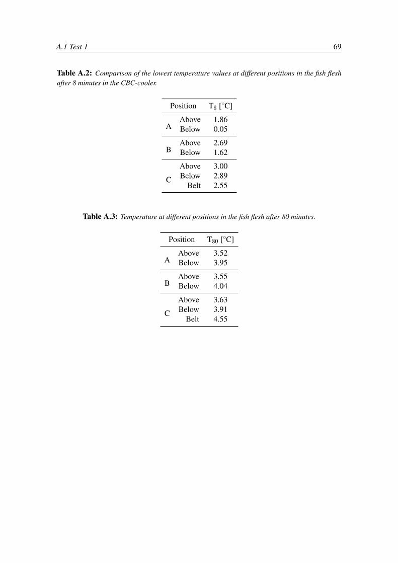
A.1 Test 1 69
Table A.2: Comparison of the lowest temperature values at different positions in the fish fleshafter 8 minutes in the CBC-cooler.
Position T8 [◦C]
AAbove 1.86Below 0.05
BAbove 2.69Below 1.62
C
Above 3.00Below 2.89
Belt 2.55
Table A.3: Temperature at different positions in the fish flesh after 80 minutes.
Position T80 [◦C]
AAbove 3.52Below 3.95
BAbove 3.55Below 4.04
C
Above 3.63Below 3.91
Belt 4.55
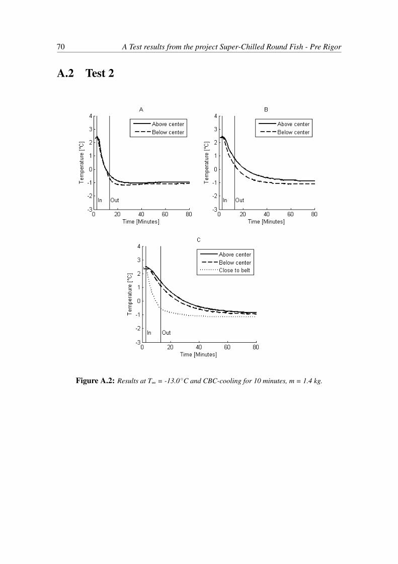
70 A Test results from the project Super-Chilled Round Fish - Pre Rigor
A.2 Test 2
Figure A.2: Results at T∞ = -13.0 ◦C and CBC-cooling for 10 minutes, m = 1.4 kg.
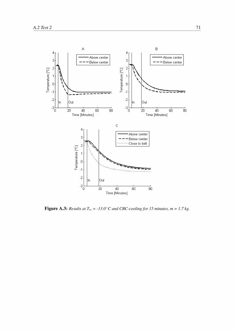
A.2 Test 2 71
Figure A.3: Results at T∞ = -13.0 ◦C and CBC-cooling for 15 minutes, m = 1.7 kg.
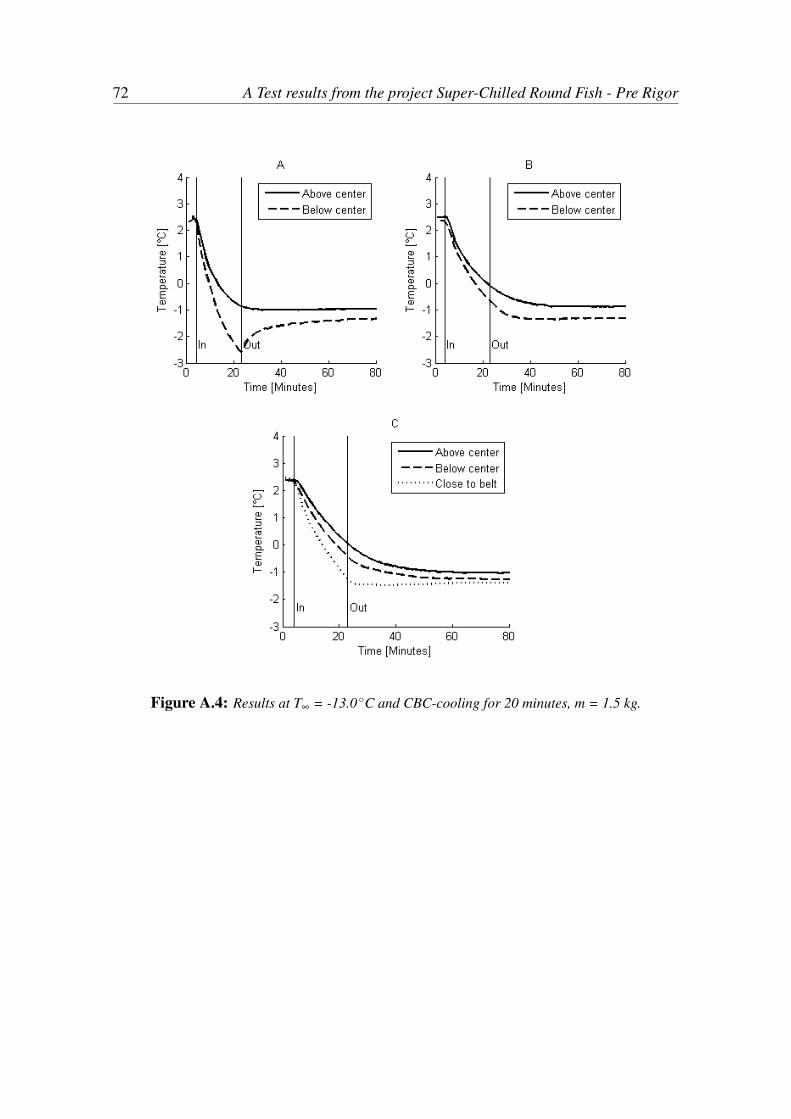
72 A Test results from the project Super-Chilled Round Fish - Pre Rigor
Figure A.4: Results at T∞ = -13.0 ◦C and CBC-cooling for 20 minutes, m = 1.5 kg.
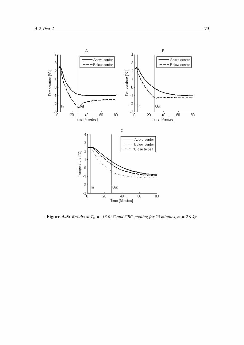
A.2 Test 2 73
Figure A.5: Results at T∞ = -13.0 ◦C and CBC-cooling for 25 minutes, m = 2.9 kg.
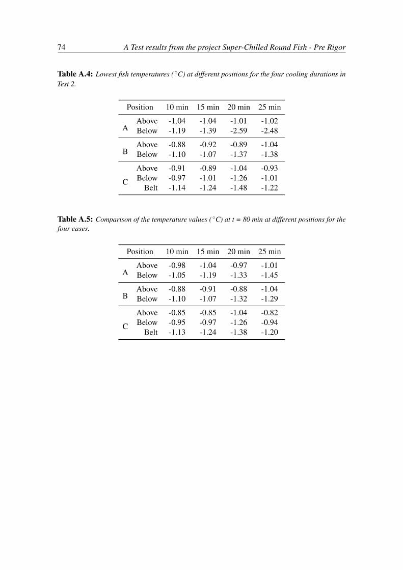
74 A Test results from the project Super-Chilled Round Fish - Pre Rigor
Table A.4: Lowest fish temperatures ( ◦C) at different positions for the four cooling durations inTest 2.
Position 10 min 15 min 20 min 25 min
AAbove -1.04 -1.04 -1.01 -1.02Below -1.19 -1.39 -2.59 -2.48
BAbove -0.88 -0.92 -0.89 -1.04Below -1.10 -1.07 -1.37 -1.38
C
Above -0.91 -0.89 -1.04 -0.93Below -0.97 -1.01 -1.26 -1.01
Belt -1.14 -1.24 -1.48 -1.22
Table A.5: Comparison of the temperature values ( ◦C) at t = 80 min at different positions for thefour cases.
Position 10 min 15 min 20 min 25 min
AAbove -0.98 -1.04 -0.97 -1.01Below -1.05 -1.19 -1.33 -1.45
BAbove -0.88 -0.91 -0.88 -1.04Below -1.10 -1.07 -1.32 -1.29
C
Above -0.85 -0.85 -1.04 -0.82Below -0.95 -0.97 -1.26 -0.94
Belt -1.13 -1.24 -1.38 -1.20
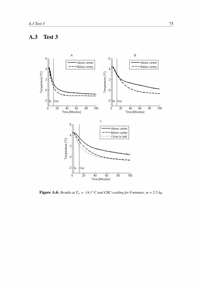
A.3 Test 3 75
A.3 Test 3
Figure A.6: Results at T∞ = -14.1 ◦C and CBC-cooling for 8 minutes, m = 2.5 kg.
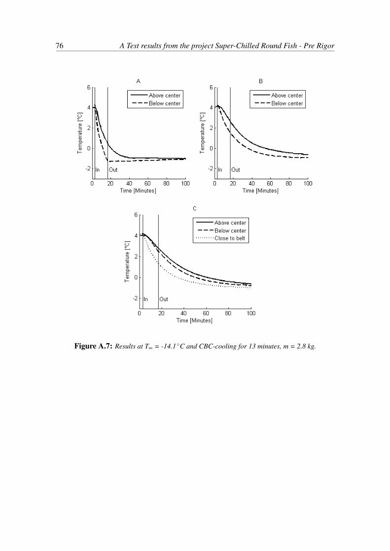
76 A Test results from the project Super-Chilled Round Fish - Pre Rigor
Figure A.7: Results at T∞ = -14.1 ◦C and CBC-cooling for 13 minutes, m = 2.8 kg.
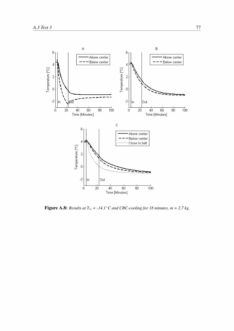
A.3 Test 3 77
Figure A.8: Results at T∞ = -14.1 ◦C and CBC-cooling for 18 minutes, m = 2.7 kg.
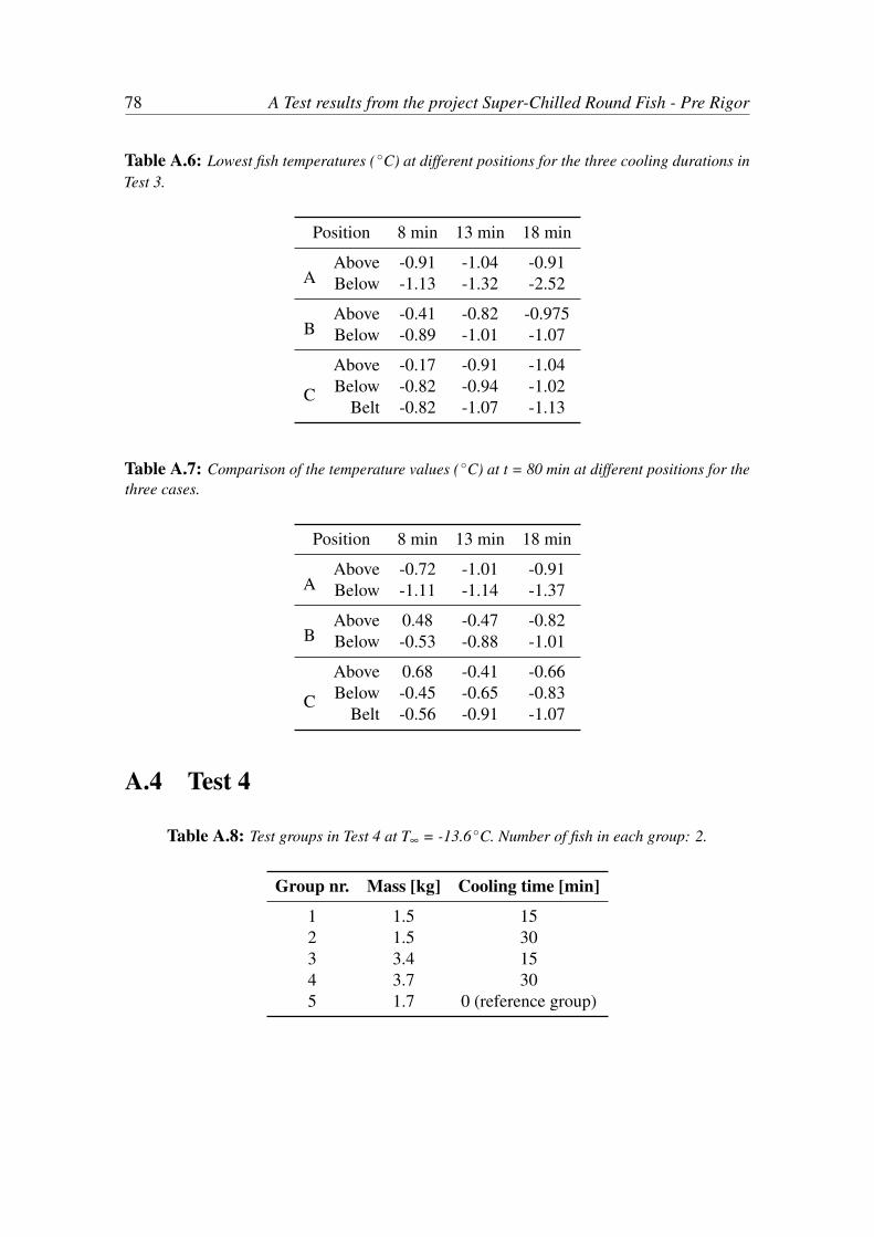
78 A Test results from the project Super-Chilled Round Fish - Pre Rigor
Table A.6: Lowest fish temperatures ( ◦C) at different positions for the three cooling durations inTest 3.
Position 8 min 13 min 18 min
AAbove -0.91 -1.04 -0.91Below -1.13 -1.32 -2.52
BAbove -0.41 -0.82 -0.975Below -0.89 -1.01 -1.07
C
Above -0.17 -0.91 -1.04Below -0.82 -0.94 -1.02
Belt -0.82 -1.07 -1.13
Table A.7: Comparison of the temperature values ( ◦C) at t = 80 min at different positions for thethree cases.
Position 8 min 13 min 18 min
AAbove -0.72 -1.01 -0.91Below -1.11 -1.14 -1.37
BAbove 0.48 -0.47 -0.82Below -0.53 -0.88 -1.01
C
Above 0.68 -0.41 -0.66Below -0.45 -0.65 -0.83
Belt -0.56 -0.91 -1.07
A.4 Test 4
Table A.8: Test groups in Test 4 at T∞ = -13.6 ◦C. Number of fish in each group: 2.
Group nr. Mass [kg] Cooling time [min]
1 1.5 152 1.5 303 3.4 154 3.7 305 1.7 0 (reference group)
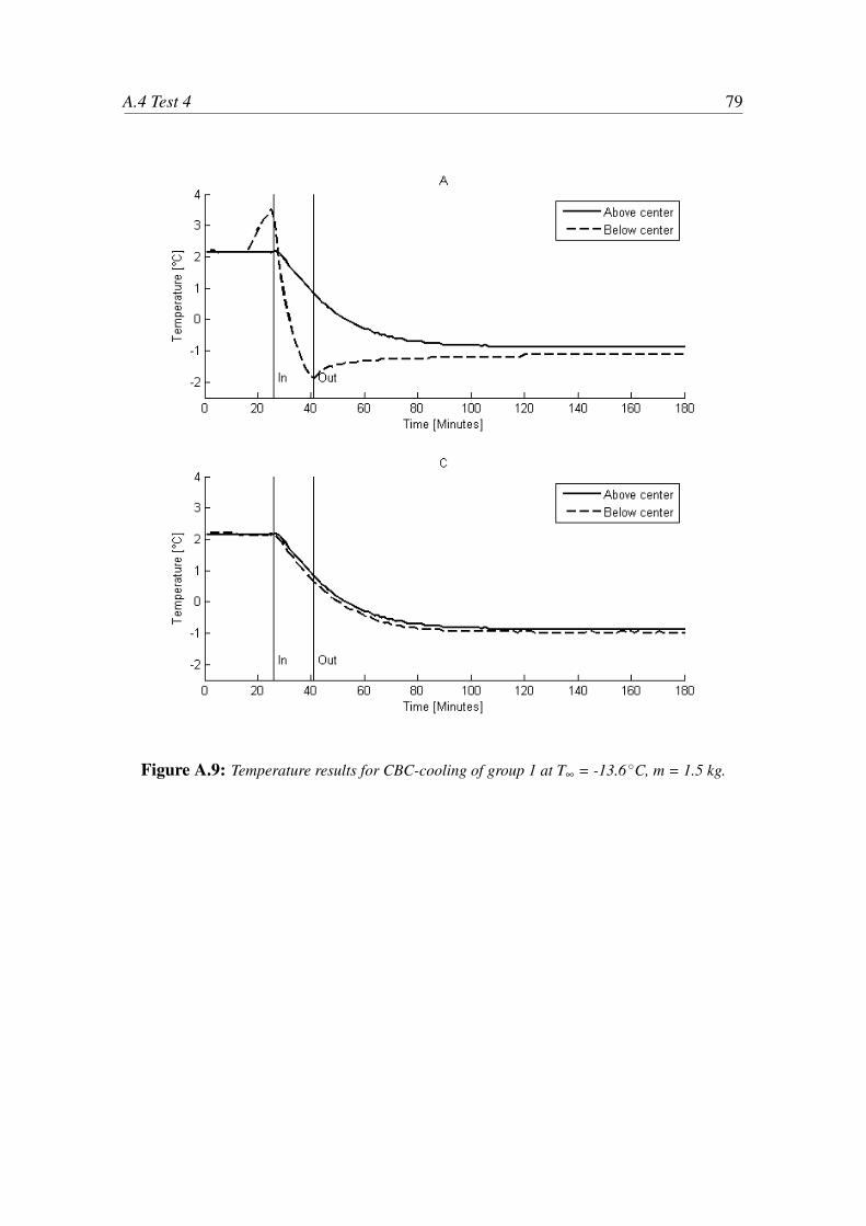
A.4 Test 4 79
Figure A.9: Temperature results for CBC-cooling of group 1 at T∞ = -13.6 ◦C, m = 1.5 kg.
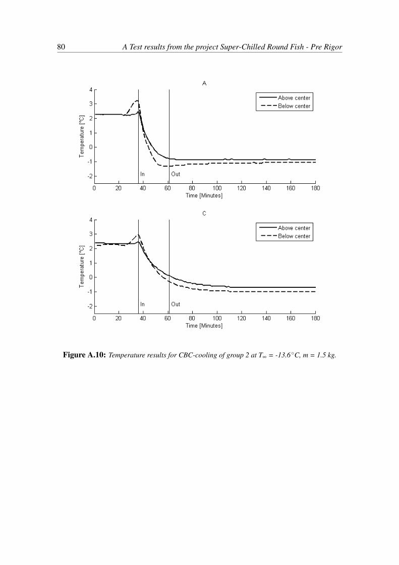
80 A Test results from the project Super-Chilled Round Fish - Pre Rigor
Figure A.10: Temperature results for CBC-cooling of group 2 at T∞ = -13.6 ◦C, m = 1.5 kg.
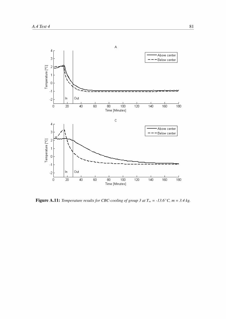
A.4 Test 4 81
Figure A.11: Temperature results for CBC-cooling of group 3 at T∞ = -13.6 ◦C, m = 3.4 kg.
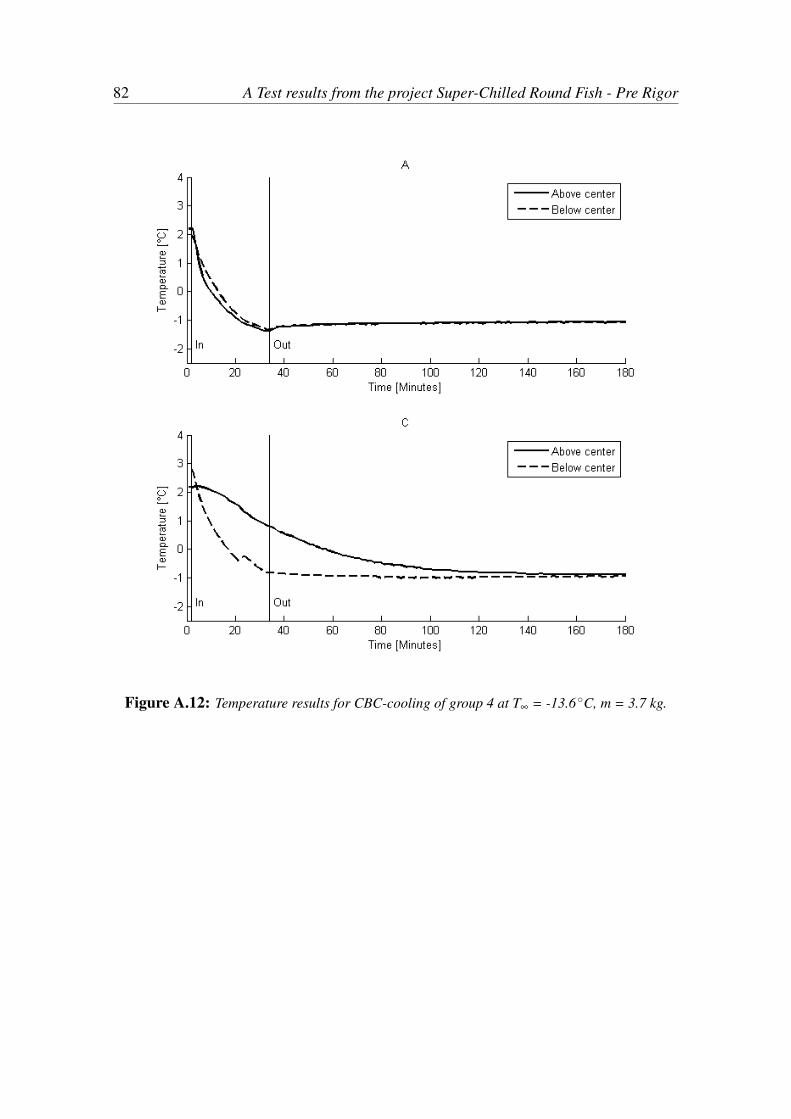
82 A Test results from the project Super-Chilled Round Fish - Pre Rigor
Figure A.12: Temperature results for CBC-cooling of group 4 at T∞ = -13.6 ◦C, m = 3.7 kg.
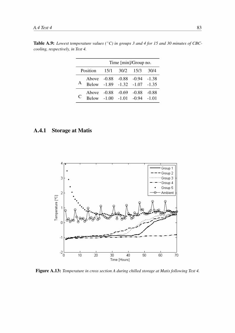
A.4 Test 4 83
Table A.9: Lowest temperature values ( ◦C) in groups 3 and 4 for 15 and 30 minutes of CBC-cooling, respectively, in Test 4.
Time [min]/Group no.
Position 15/1 30/2 15/3 30/4
AAbove -0.88 -0.88 -0.94 -1.38Below -1.89 -1.32 -1.07 -1.35
CAbove -0.88 -0.69 -0.88 -0.88Below -1.00 -1.01 -0.94 -1.01
A.4.1 Storage at Matis
Figure A.13: Temperature in cross section A during chilled storage at Matis following Test 4.
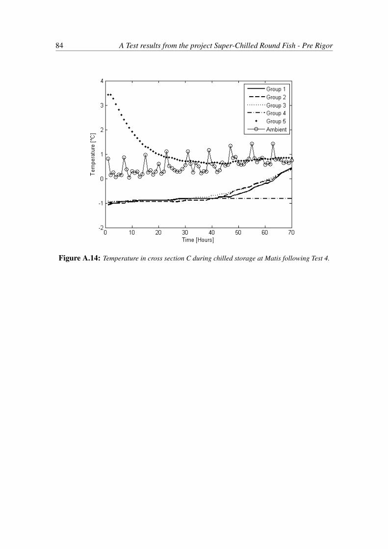
84 A Test results from the project Super-Chilled Round Fish - Pre Rigor
Figure A.14: Temperature in cross section C during chilled storage at Matis following Test 4.

DTU Mechanical Engineering
Section of Fluid Mechanics, Coastal and Maritime Engineering
Technical University of Denmark
Nils Koppels Allé, Bld. 403
DK- 2800 Kgs. Lyngby
Denmark
Phone (+45) 45 25 13 60
Fax (+45) 45 88 43 25
www.mek.dtu.dk