Embed Size (px)
Citation preview
UNIVERSITY OF ZAGREB FACULTY OF MECHANICAL ENGINEERING AND NAVAL ARCHITECTURE
MASTER THESIS
Tessa Uroić
Zagreb, 2014
UNIVERSITY OF ZAGREB FACULTY OF MECHANICAL ENGINEERING AND NAVAL ARCHITECTURE
MASTER THESIS Optimisation under uncertainty and constraints of a
tube bundle heat exchanger
Supervisors: Student:
Prof. Hrvoje Jasak Tessa Uroić Dr. Henrik Rusche
Zagreb, 2014

Tessa Uroić Master Thesis
I hereby declare that this thesis is entirely the result of my own work except where
otherwise indicated. I have fully cited all used sources and I have only used the ones
given in the list of references.
I would like to express my sincere gratitude to my supervisors, Prof. Hrvoje Jasak
and Dr. Henrik Rusche, who have given me many valuable comments, supported me
throughout my thesis and allowed me to explore and work in my own way.
I am also grateful to Prof. Zvonimir Guzović for his continuous support and
mentorship during my studies.
Finally, I would like to thank my colleague and partner Vanja Škurić, for his
immense patience, help and love.
_____________________________________________________________________________________ Faculty of Mechanical Engineering and Naval Architecture II
Tessa Uroić Master Thesis
Contents 1. Introduction ........................................................................................................... 1
2. Probability ............................................................................................................. 2
2.1. Definition of Probability ........................................................................... 2
2.1.1. Frequentistic Definition ................................................................ 2
2.1.2. Classical Definition ...................................................................... 2
2.1.3. Bayesian Definition ...................................................................... 3
2.2. Sample Space and Events ......................................................................... 4
2.3. The Three Axioms of Probability Theory ................................................. 4
2.4. Conditional Probability ............................................................................. 5
2.5. Characteristics of the Data ........................................................................ 6
2.5.1. Central Measures .......................................................................... 6
2.5.2. Dispersion Measures .................................................................... 7
2.5.3. Other Measures ............................................................................ 7
2.5.4. Measures of Correlation ............................................................... 8
2.6. Uncertainty Modeling ............................................................................. 10
2.6.1. Random Variables ...................................................................... 10
2.7. Methods of Reliability ............................................................................ 20
2.7.1. Failure Events and Basic Random Variables ............................. 20
2.7.2. Linear Limit State Functions and Normal Distributed Variables21
2.7.3. The Error Propagation Law ........................................................ 23
2.7.4. Non-linear Limit State Functions ............................................... 25
2.7.5. Sampling Methods ...................................................................... 27
3. Dakota Software Package and Optimization Capabilities .................................. 30
3.1. Optimization ........................................................................................... 31
3.1.1. Optimization Formulations ........................................................ 32
3.1.2. Optimization Methods ................................................................ 34
3.2. Optimization Under Uncertainty ............................................................. 36
3.2.1. Uncertain Variables .................................................................... 37
3.3. Uncertainty Quantification ...................................................................... 38
3.3.1. Sampling Methods ...................................................................... 39
3.3.2. Reliability methods .................................................................... 42
4. Multi-objective Optimization ............................................................................. 47
_____________________________________________________________________________________ Faculty of Mechanical Engineering and Naval Architecture III
Tessa Uroić Master Thesis
4.1. Aggregating Functions ............................................................................ 50
4.2. Multi-objective Optimization Algorithm MOGA and Pareto Front ....... 50
5. Tube Bank Heat Exchanger Problem ................................................................. 54
5.1. Problem Parameters ................................................................................ 55
6. Results and discussion ........................................................................................ 63
6.1. Multi-objective Genetic Algorithm Options ........................................... 63
6.2. Uncertainty Quantification ...................................................................... 73
6.2.1. Uncertainty Analysis of Design 1 with Relaxed Constraints ..... 74
6.2.2. Uncertainty Analysis of Design 2 and Design 3 with Relaxed Constraints .............................................................................................. 82
6.2.3. Uncertainty Analysis of Designs with Strong Constraints ......... 90
7. Conclusion .......................................................................................................... 95
_____________________________________________________________________________________ Faculty of Mechanical Engineering and Naval Architecture IV
Tessa Uroić Master Thesis
List of figures
Figure 1 Venn diagrams illustrating the union of events (left) and the intersection of events (right) [4] .... 4
Figure 2 Illustration of skewness ................................................................................................................. 8
Figure 3 Illustration of kurtosis ................................................................................................................... 8
Figure 4 Two examples of paired data sets [1] ............................................................................................ 9
Figure 5 Illustration of A) a cumulative distribution function and B) a probability density function for a continuous random variable [4] .................................................................................................................. 12
Figure 6 Illustration of A) a cumulative distribution function and B) a probability density function for a discrete random variable [4] ....................................................................................................................... 12
Figure 7 Illustration of probability density and cumulative distribution functions for different distribution types. Mean 𝜇 = 160 and standard deviation 𝜎 = 40 are the same for all the distributions except the Exponential distribution for which the expected value and the variance are equal [4] .............................. 16
Figure 8 Example of the density and distribution function of a normally distributed random variable defined by the parameters 𝜇 = 160 and 𝜎 = 40 [4] .................................................................................. 17
Figure 9 Illustration of the relationship between a Normal distributed random variable and a standard Normal distributed random variable [4] ..................................................................................................... 18
Figure 10 Double sided and symmetrical 1 − 𝛼 confidence interval on the mean value [4] ..................... 19
Figure 11 Illustration of the two-dimensional case of a linear limit state function and Normal distributed variables 𝑥 [4] ............................................................................................................................................. 22
Figure 12 Illustration of the error propagation law: The transformation of the density function 𝑓𝑌(𝑦) according to the relation 𝑦 = 𝑔(𝑥) and the linear approximation of the relation between the two random variables [4] ................................................................................................................................................ 25
Figure 13 Illustration of the linearization proposed by Hasofer and Lind [5] in standard normal space [4] .................................................................................................................................................................... 27
Figure 14 An example of Latin Hypercube sampling with four bins in design parameters 𝑥1 and 𝑥2. The dots are the sample sites. [7] ....................................................................................................................... 41
Figure 15 Distribution of input sample points for Monte Carlo ∆ and Latin Hypercube + sampling for number of samples equal to 5 and 10 [7] .................................................................................................... 42
Figure 16 Graphical depiction of calculation of cumulative distribution function in the original uncertain variable space [7] ........................................................................................................................................ 43
Figure 17 Graphical depiction of integration for the calculation of cumulative distribution function in the transformed uncertain variable space [7] .................................................................................................... 44
Figure 18 Example for the rank of 10 individuals and the corresponding probability to participate in the reproduction process, represented on a circular diagram [9] ...................................................................... 49
Figure 19 Schematic representation of the concept of Pareto optimal front [9] ........................................ 51
Figure 20 The domain is divided into three zones ..................................................................................... 54
Figure 21 The optimization workflow [1] .................................................................................................. 56
Figure 22 The loosely-coupled interface between Dakota and a simulation code [7] ............................... 57
Figure 23 The dimensions of the computational domain .......................................................................... 58
_____________________________________________________________________________________ Faculty of Mechanical Engineering and Naval Architecture V
Tessa Uroić Master Thesis
Figure 24 An example of computational mesh .......................................................................................... 59
Figure 25 Boundary conditions ................................................................................................................. 59
Figure 26 Depiction of cyclicAMI boundary condition ............................................................................ 60
Figure 27 Temperature field of one of the optimal solutions .................................................................... 61
Figure 28 Pressure field of one of the optimal solutions ........................................................................... 61
Figure 29 Domain for the strong constraints [1] ....................................................................................... 63
Figure 30 A comparison of different number of generations, each generation has 40 members ............... 64
Figure 31 A comparison of different number of generations, each generation has 80 members ............... 65
Figure 32 A comparison of two cases with approximately the same number of evaluations .................... 66
Figure 33 A comparison of two cases with approximately the same number of evaluations .................... 67
Figure 34 A comparison of different mutation rates for strong and relaxed constraints ........................... 68
Figure 35 Pareto fronts for relaxed and strong constraints ........................................................................ 69
Figure 36 A comparison of different crossover rates ................................................................................ 70
Figure 37 Custom design 1 – temperature and pressure field .................................................................... 71
Figure 38 Custom design 2 – temperature and pressure field .................................................................... 71
Figure 39 Custom design 3 – temperature and pressure field .................................................................... 72
Figure 40 Pareto front and three points corresponding to three custom designs ....................................... 73
Figure 41 The black triangle denotes Design 1 point on the Pareto front ................................................. 74
Figure 42 Temperature field of Design 1 ................................................................................................... 74
Figure 43 Pressure field of Design 1 ......................................................................................................... 75
Figure 44 The normal distribution of 𝑥137T .................................................................................................. 75
Figure 45 The normal distribution of 𝑦137T .................................................................................................. 76
Figure 46 Cumulative distribution function for pressure drop (Design 1)................................................. 77
Figure 47 Relative density function for pressure drop (method: Latin Hypercube sampling) ................... 79
Figure 48 Relative density function for pressure drop (method: Monte Carlo sampling) ......................... 79
Figure 49 Distribution of the uncertain variable, 𝑇𝑤𝑎𝑙𝑙37T ............................................................................ 80
Figure 50 Cumulative distribution function for temperature increase (Design 1) ..................................... 81
Figure 51 Density value for temperature increase ..................................................................................... 81
Figure 52 The green triangle denotes Design 2 point and the red triangle denotes Design 3 on the Pareto front ............................................................................................................................................................ 82
Figure 53 Temperature field of Design 2 .................................................................................................. 82
Figure 54 Pressure field of Design 2 ......................................................................................................... 83
Figure 55 Temperature field of Design 3 .................................................................................................. 83
Figure 56 Pressure field of Design 3 ......................................................................................................... 83
Figure 57 Cumulative distribution function for pressure drop (Design 2)................................................. 84
_____________________________________________________________________________________ Faculty of Mechanical Engineering and Naval Architecture VI

Tessa Uroić Master Thesis
Figure 58 Cumulative distribution function for pressure drop (Design 3)................................................. 84
Figure 59 Relative density function for pressure drop (method: Latin Hypercube sampling, Design 2) .. 85
Figure 60 Relative density function for pressure drop (method: LHS, Design 3) ..................................... 86
Figure 61 Relative density function for pressure drop with finer mesh (10000 cells) for Design 3 .......... 86
Figure 62 Cumulative distribution function for temperature increase (Design 2) ..................................... 87
Figure 63 Cumulative distribution function for temperature increase (Design 3) ..................................... 88
Figure 64 Density value for temperature increase (Design 2) ................................................................... 88
Figure 65 Density value for temperature increase (Design 3) ................................................................... 89
Figure 66 The positions of the three designs from [1] on the corresponding Pareto fronts ....................... 90
Figure 67 Temperature and pressure field of Design 1 ............................................................................. 91
Figure 68 Temperature and pressure field of Design 2 ............................................................................. 91
Figure 69 Temperature and pressure field of Design 3 ............................................................................. 92
_____________________________________________________________________________________ Faculty of Mechanical Engineering and Naval Architecture VII
Tessa Uroić Master Thesis
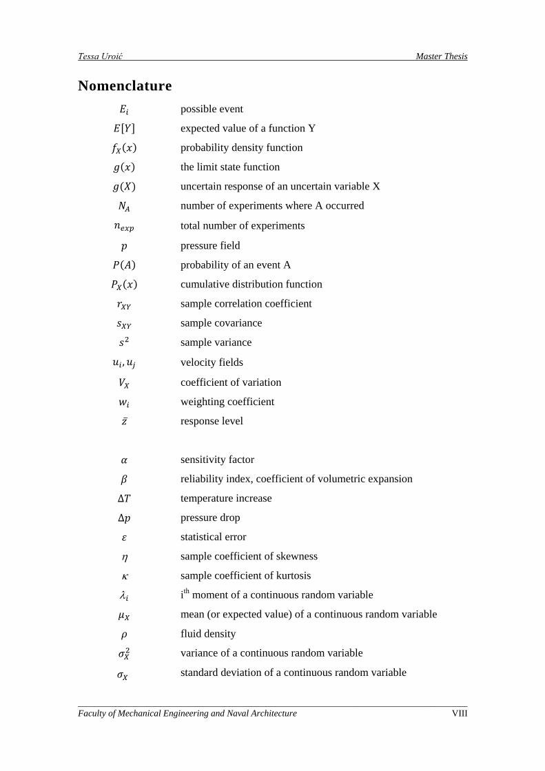
Nomenclature 𝐸𝑖 possible event
𝐸[𝑌] expected value of a function Y
𝑓𝑋(𝑥) probability density function
𝑔(𝑥) the limit state function
𝑔(𝑋) uncertain response of an uncertain variable X
𝑁𝐴 number of experiments where A occurred
𝑛𝑒𝑥𝑝 total number of experiments
𝑝 pressure field
𝑃(𝐴) probability of an event A
𝑃𝑋(𝑥) cumulative distribution function
𝑟𝑋𝑌 sample correlation coefficient
𝑠𝑋𝑌 sample covariance
𝑠2 sample variance
𝑢𝑖 ,𝑢𝑗 velocity fields
𝑉𝑋 coefficient of variation
𝑤𝑖 weighting coefficient
𝑧̅ response level
𝛼 sensitivity factor
𝛽 reliability index, coefficient of volumetric expansion
∆𝑇 temperature increase
∆𝑝 pressure drop
𝜀 statistical error
η sample coefficient of skewness
κ sample coefficient of kurtosis
λ𝑖 ith moment of a continuous random variable
𝜇𝑋 mean (or expected value) of a continuous random variable
𝜌 fluid density
𝜎𝑋2 variance of a continuous random variable
𝜎𝑋 standard deviation of a continuous random variable
_____________________________________________________________________________________ Faculty of Mechanical Engineering and Naval Architecture VIII
Tessa Uroić Master Thesis
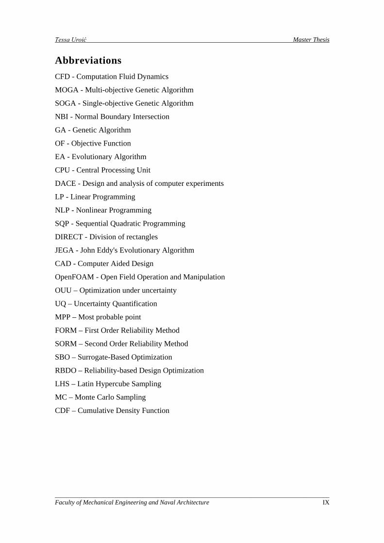
Abbreviations CFD - Computation Fluid Dynamics
MOGA - Multi-objective Genetic Algorithm
SOGA - Single-objective Genetic Algorithm
NBI - Normal Boundary Intersection
GA - Genetic Algorithm
OF - Objective Function
EA - Evolutionary Algorithm
CPU - Central Processing Unit
DACE - Design and analysis of computer experiments
LP - Linear Programming
NLP - Nonlinear Programming
SQP - Sequential Quadratic Programming
DIRECT - Division of rectangles
JEGA - John Eddy's Evolutionary Algorithm
CAD - Computer Aided Design
OpenFOAM - Open Field Operation and Manipulation
OUU – Optimization under uncertainty
UQ – Uncertainty Quantification
MPP – Most probable point
FORM – First Order Reliability Method
SORM – Second Order Reliability Method
SBO – Surrogate-Based Optimization
RBDO – Reliability-based Design Optimization
LHS – Latin Hypercube Sampling
MC – Monte Carlo Sampling
CDF – Cumulative Density Function
_____________________________________________________________________________________ Faculty of Mechanical Engineering and Naval Architecture IX
Tessa Uroić Master Thesis
Abstract Optimization is a discipline of numerical mathematics which aims to improve the
operation of a system or process as good as possible in some defined sense.
Optimization algorithms work to minimize (or maximize) an objective function,
typically calculated by the user simulation code, subject to constraints on design
variables and responses.
Parameters and settings of tube bank heat exchanger multi-objective optimization
are described. The problem consists of finding the best locations of the tubes to increase
heat exchange (i.e. the temperature increase of the fluid) while at the same time limit the
pressure loss. The two corresponding numerical parameters to optimize are the average
temperature difference ∆𝑇 and pressure drop ∆𝑝 between inflow and outflow.
The set of coupled numerical tools to solve the multi-objective optimization
consists of open source optimization software Dakota, open source CFD toolbox
OpenFOAM and open source software for geometry creation Salome. Multi-objective
Genetic Algorithm is used to obtain optimal designs.
Results of the optimization process are presented on corresponding Pareto fronts.
Different parameters of the Multi-objective Genetic Algorithm are examined and
discussed.
Uncertainty quantification or nondeterministic analysis is the process of
characterizing input uncertainties, forward propagating these uncertainties through a
computational model, and performing statistical or interval assessments on the resulting
responses. Uncertainty quantification is related to sensitivity analysis in that the
common goal is to gain an understanding of how variations in the parameters affect the
response functions of the engineering design problem. For uncertainty quantification,
some or all of the components of the parameter vector, are considered to be uncertain as
specified by particular probability distributions.
Effect of uncertain tube coordinates and uncertain tubes’ temperature is examined
and presented in graphs and histograms.
Three optimal points from [1] are chosen and their robustness evaluated by means
of the uncertainty quantification methods.
Key words: optimization under uncertainty, constraints, multi-objective
optimization, computational fluid dynamics
_____________________________________________________________________________________ Faculty of Mechanical Engineering and Naval Architecture X

Tessa Uroić Master Thesis
Sažetak Optimizacija je disciplina numeričke matematike za unaprijeđivanje rada sustava
ili procesa da bi rezultati bili najbolji mogući. Optimizacijski algoritmi za zadaću imaju
minimizaciju ili maksimizaciju funkcije cilja koja se proračunava simulacijom, uz
odgovarajuća ograničenja varijabli.
U radu su opisani parametri i postavke optimizacije po višestrukim funkcijama
cilja sa ograničenjima varijabli cijevnog izmjenjivača topline. Traže se optimalne
pozicije cijevi kako bi se povećao prirast temperature fluida uz što manji pad tlaka u
izmjenjivaču. temperaturni prirast i pad tlaka su ujedno i funkcije cilja za ovaj problem.
Za optimizaciju su korištena tri računalna alata: open source alat Salome za
konstrukciju geometrije, open source paket za računalnu dinamiku fluida OpenFOAM i
open source software za optimizaciju Dakota.
Ispitivani su različiti parametri genetskog algoritma za optimizaciju po
višestrukim funkcijama cilja te su rezultati prikazani preko Pareto linija.
Provedena je i kvantifikacija nesigurnosti varijabli – ispitivano je kako male
promjene u varijablama, koje su zadane normalnom raspodjelom, utječu na promatrani
sustav, odnosno funkcije cilja.
Utjecaj nesigurnih koordinata jedne cijevi i nesigurne temperature stijenki cijevi
prikazan je kumulativnim distribucijama i histogramima.
Ključne riječi: optimizacija, nesigurnost varijabli, višestruke funkcije cilja
_____________________________________________________________________________________ Faculty of Mechanical Engineering and Naval Architecture XI
Tessa Uroić Master Thesis
Prošireni sažetak Optimizacija je disciplina numeričke matematike za unaprijeđivanje rada sustava
ili procesa da bi rezultati bili najbolji mogući. Optimizacijski algoritmi za zadaću imaju
minimizaciju ili maksimizaciju funkcije cilja koja se proračunava simulacijom, uz
odgovarajuća ograničenja varijabli.
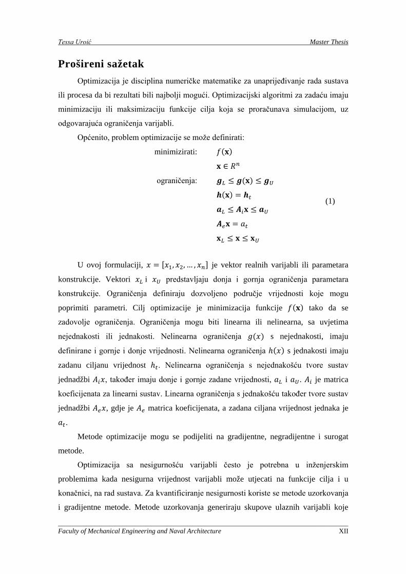
Općenito, problem optimizacije se može definirati:
minimizirati: 𝑓(𝐱)
𝐱 ∈ 𝑅𝑛
ograničenja: 𝒈𝐿 ≤ 𝒈(𝐱) ≤ 𝒈𝑈
𝒉(𝐱) = 𝒉𝑡
𝒂𝐿 ≤ 𝑨𝑖𝐱 ≤ 𝒂𝑈
𝑨𝑒𝐱 = 𝑎𝑡
𝐱𝐿 ≤ 𝐱 ≤ 𝐱𝑈
(1)
U ovoj formulaciji, 𝑥 = [𝑥1, 𝑥2, … , 𝑥𝑛] je vektor realnih varijabli ili parametara
konstrukcije. Vektori 𝑥𝐿 i 𝑥𝑈 predstavljaju donja i gornja ograničenja parametara
konstrukcije. Ograničenja definiraju dozvoljeno područje vrijednosti koje mogu
poprimiti parametri. Cilj optimizacije je minimizacija funkcije 𝑓(𝐱) tako da se
zadovolje ograničenja. Ograničenja mogu biti linearna ili nelinearna, sa uvjetima
nejednakosti ili jednakosti. Nelinearna ograničenja 𝑔(𝑥) s nejednakosti, imaju
definirane i gornje i donje vrijednosti. Nelinearna ograničenja ℎ(𝑥) s jednakosti imaju
zadanu ciljanu vrijednost ℎ𝑡. Nelinearna ograničenja s nejednakošću tvore sustav
jednadžbi 𝐴𝑖𝑥, također imaju donje i gornje zadane vrijednosti, 𝑎𝐿 i 𝑎𝑈. 𝐴𝑖 je matrica
koeficijenata za linearni sustav. Linearna ograničenja s jednakošću također tvore sustav
jednadžbi 𝐴𝑒𝑥, gdje je 𝐴𝑒 matrica koeficijenata, a zadana ciljana vrijednost jednaka je
𝑎𝑡.
Metode optimizacije mogu se podijeliti na gradijentne, negradijentne i surogat
metode.
Optimizacija sa nesigurnošću varijabli često je potrebna u inženjerskim
problemima kada nesigurna vrijednost varijabli može utjecati na funkcije cilja i u
konačnici, na rad sustava. Za kvantificiranje nesigurnosti koriste se metode uzorkovanja
i gradijentne metode. Metode uzorkovanja generiraju skupove ulaznih varijabli koje
_____________________________________________________________________________________ Faculty of Mechanical Engineering and Naval Architecture XII
Tessa Uroić Master Thesis
odgovaraju raspodjeli koju zadaje korisnik, procjenjuju vrijednost funkcije cilja te
smještaju konstrukciju u odgovarajući interval vrijednosti funkcije cilja. Za funkciju
cilja računaju se srednja vrijednost, standardna devijacija, intervali pouzdanosti te se
dobiva kumulativna raspodjela vjerojatnosti.
Gradijentne metode nazivaju se i metodama za procjenu pouzdanosti, a njihova
upotreba je uglavnom računalno manje zahtjevna od upotrebe metoda uzorkovanja. Ove
su metode bolje i u računanju statističkih podataka za događaje manje vjerojatnosti.
„Za zadani skup nesigurnih ulaznih varijabli, X, i zadane realne vrijednosti
mogućih odgovora sustava, g, koja je vjerojatnost da će funkcija cilja biti manja ili
jednaka nekoj vrijednosti, 𝑧̅?” To se pitanje matematički može zapisati: 𝑃[𝑔(𝑋) ≤ 𝑧̅] =
𝐹𝑔(𝑧̅), gdje je 𝐹𝑔(𝑧̅) kumulativna raspodjela vjerojatnosti nesigurnog odgovora
(vrijednosti funkcije cilja) 𝑔(𝑋).
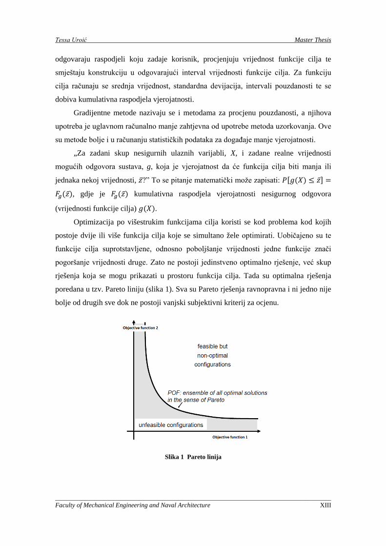
Optimizacija po višestrukim funkcijama cilja koristi se kod problema kod kojih
postoje dvije ili više funkcija cilja koje se simultano žele optimirati. Uobičajeno su te
funkcije cilja suprotstavljene, odnosno poboljšanje vrijednosti jedne funkcije znači
pogoršanje vrijednosti druge. Zato ne postoji jedinstveno optimalno rješenje, već skup
rješenja koja se mogu prikazati u prostoru funkcija cilja. Tada su optimalna rješenja
poredana u tzv. Pareto liniju (slika 1). Sva su Pareto rješenja ravnopravna i ni jedno nije
bolje od drugih sve dok ne postoji vanjski subjektivni kriterij za ocjenu.
Slika 1 Pareto linija
_____________________________________________________________________________________ Faculty of Mechanical Engineering and Naval Architecture XIII
Tessa Uroić Master Thesis
Za dobivanje Pareto rješenja, koristi se evolucijski algoritam koji se temelji na
Darwinovim postavkama teorije evolucije. „Geni“ (karakteristike) mogućih
konstrukcijskih rješenja križaju se i mutiraju. Takvim postupcima dobivaju se nova
rješenja, čije se performanse uspoređuju s performansama drugih konstrukcijskih
rješenja. Početna se rješenja određuju u inicijalnoj populaciji sa određenim brojem
članova, od kojih se zatim dio križa ili mutira određenom brzinom te nastaje nova
populacija. U novoj populaciji preživljavaju samo dominantni članovi, tj. oni čije su
performanse bolje. Tako se, kroz određeni broj populacija, određuju najjači članovi –
konstrukcije čije su se performanse pokazale najboljima.
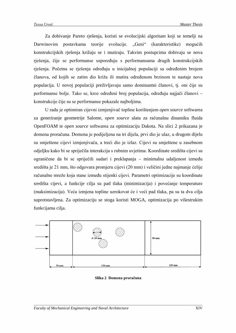
U radu je optimiran cijevni izmjenjivač topline korištenjem open source softwarea
za generiranje geometrije Salome, open source alata za računalnu dinamiku fluida
OpenFOAM te open source softwarea za optimizaciju Dakota. Na slici 2 prikazana je
domena proračuna. Domena je podijeljena na tri dijela, prvi dio je ulaz, u drugom dijelu
su smještene cijevi izmjenjivača, a treći dio je izlaz. Cijevi su smještene u zasebnom
odjeljku kako bi se spriječila interakcija s rubnim uvjetima. Koordinate središta cijevi su
ograničene da bi se spriječili sudari i preklapanja – minimalna udaljenost između
središta je 21 mm, što odgovara promjeru cijevi (20 mm) i veličini jedne najmanje ćelije
računalne mreže koja stane između stijenki cijevi. Parametri optimizacije su koordinate
središta cijevi, a funkcije cilja su pad tlaka (minimizacija) i povećanje temperature
(maksimizacija). Veća izmjena topline uzrokovat će i veći pad tlaka, pa su ta dva cilja
suprotstavljena. Za optimizaciju se stoga koristi MOGA, optimizacija po višestrukim
funkcijama cilja.
Slika 2 Domena proračuna
_____________________________________________________________________________________ Faculty of Mechanical Engineering and Naval Architecture XIV
Tessa Uroić Master Thesis
Zrak ulazi u domenu s temperaturom 𝑇𝑖𝑛𝑙𝑒𝑡 = 293 K i zagrijava se prolazeći
između cijevi. Temperatura stijenki cijevi je konstantna, 𝑇𝑤𝑎𝑙𝑙 = 353 K. Reynoldsov
broj jednak je 14 kako bi se osiguralo laminarno i stacionarno strujanje, a definiran je za
dimenziju promjera cijevi i ulaznu brzinu 𝑣𝑖𝑛𝑙𝑒𝑡 = 0.01 m/s. Rubni uvjeti gornje i donje
stijenke postavljeni su kao cyclicAMI jer dozvoljavaju različit broj ćelija. Tlak na izlazu
jednak je atmosferskom tlaku.
Jednadžbe koje opisuju sustav rješavaju se u OpenFOAM alatu:
Jednadžba kontinuiteta
𝜕𝜌𝜕𝑡
+𝜕(𝜌𝑢𝑖)𝜕𝑥𝑖
= 0 (2)
Jednadžba količine gibanja
𝜕(𝜌𝑢𝑖)𝜕𝑡
+𝜕�𝜌𝑢𝑖𝑢𝑗�𝜕𝑥𝑗
= 𝜌𝑔𝑖 −𝜕𝜕𝑥𝑖
�𝑝 +23𝜇𝜕𝑢𝑗𝜕𝑥𝑗
� +𝜕𝜕𝑥𝑗
�𝜇 �𝜕𝑢𝑖𝜕𝑥𝑗
+𝜕𝑢𝑗𝜕𝑥𝑖
�� (3)
Energijska jednadžba
𝜕(𝜌𝑒)𝜕𝑡
+𝜕�𝜌𝑒𝑢𝑗�𝜕𝑥𝑗
= 𝜌𝑔𝑖𝑢𝑖 −𝜕(𝑝𝑢𝑖)𝜕𝑥𝑖
−𝜕𝜕𝑥𝑗
�23𝜇𝜕𝑢𝑗𝜕𝑥𝑗
𝑢𝑖� +𝜕𝜕𝑥𝑗
�𝜇 �𝜕𝑢𝑖𝜕𝑥𝑗
+𝜕𝑢𝑗𝜕𝑥𝑖
� 𝑢𝑖� + +
+𝜕𝜕𝑥𝑗
�λ�𝜕𝑇𝜕𝑥𝑖
𝚤 +𝜕𝑇𝜕𝑥𝑗
𝚥 +𝜕𝑇𝜕𝑥𝑘
𝑘�⃗ �� + 𝜌𝑄 (4)
Evaluacija jednog skupa parametara (pozicija cijevi) uključuje sljedeće korake:
1. generiranje geometrije (cijevi) u softwareu Salome, koji koristi zadane pozicije
cijevi iz programa za optimizaciju Dakota
2. generiranje odgovarajuće domene i računalne mreže u snappyHexMeshu i
blockMeshu
3. CFD simulacija, tj. rješavanje odgovarajućih jednadžbi alatom OpenFOAM
4. izračun vrijednosti funkcija cilja (pad tlaka, povećanje temperature) koristeći
swak4Foam
_____________________________________________________________________________________ Faculty of Mechanical Engineering and Naval Architecture XV
Tessa Uroić Master Thesis
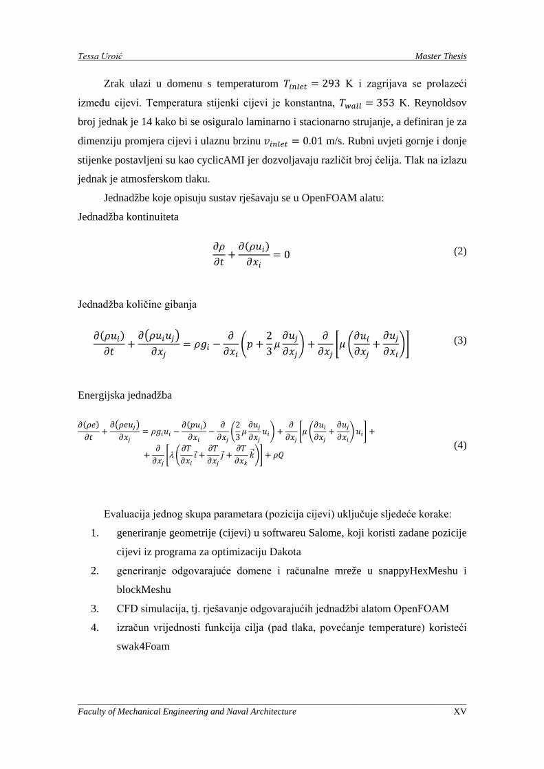
U prvom je dijelu rezultata prikazan utjecaj različitog broja generacija i veličine
populacije na izgled Pareto linije.
Slika 3 Usporedba različitog broja generacija uz konstantu veličinu populacije (40 članova)
Veći broj generacija dovodi do bolje statističke konvergencije, što je očekivano
jer je proveden veći broj evaluacija (broj evaluacija približno je jednak umnošku broja
generacija i veličine populacije), kao što je pokazano na slici 3. 20 generacija dalo je
manje padove tlaka za iste odgovarajuće promjene temperature, u usporedbi s 5 i 10
generacija. 15 generacija pokazalo je rezultate vrlo sličnima onima dobivenim za 20
generacija, pa se može zaključiti da je optimizacija s 15 generacija efikasnija jer je uz
manje evaluacija došla do istih rezultata. Također, većim brojem generacija pokriven je
širi raspon promjena temperature i tlaka, ali neka su područja rijetko pokrivena.
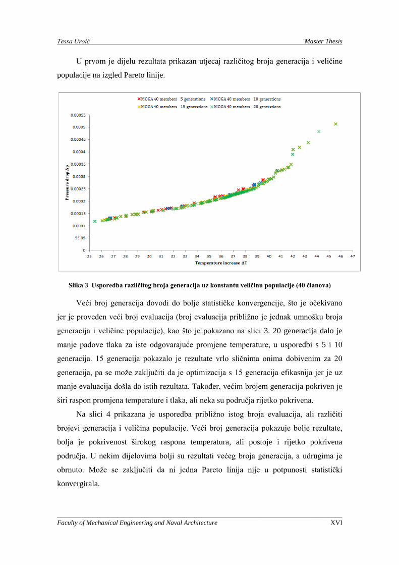
Na slici 4 prikazana je usporedba približno istog broja evaluacija, ali različiti
brojevi generacija i veličina populacije. Veći broj generacija pokazuje bolje rezultate,
bolja je pokrivenost širokog raspona temperatura, ali postoje i rijetko pokrivena
područja. U nekim dijelovima bolji su rezultati većeg broja generacija, a udrugima je
obrnuto. Može se zaključiti da ni jedna Pareto linija nije u potpunosti statistički
konvergirala.
_____________________________________________________________________________________ Faculty of Mechanical Engineering and Naval Architecture XVI
Tessa Uroić Master Thesis
Slika 4 Usporedba MOGA metode s približno istim brojem evaluacija
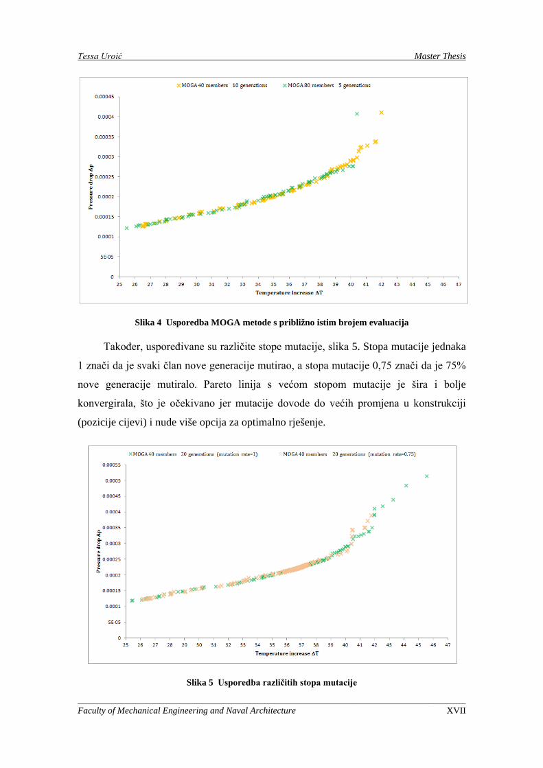
Također, uspoređivane su različite stope mutacije, slika 5. Stopa mutacije jednaka
1 znači da je svaki član nove generacije mutirao, a stopa mutacije 0,75 znači da je 75%
nove generacije mutiralo. Pareto linija s većom stopom mutacije je šira i bolje
konvergirala, što je očekivano jer mutacije dovode do većih promjena u konstrukciji
(pozicije cijevi) i nude više opcija za optimalno rješenje.
Slika 5 Usporedba različitih stopa mutacije
_____________________________________________________________________________________ Faculty of Mechanical Engineering and Naval Architecture XVII
Tessa Uroić Master Thesis
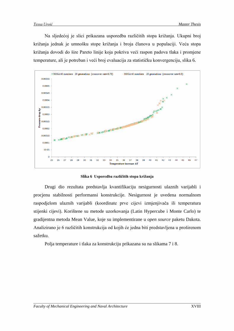
Na sljedećoj je slici prikazana usporedba različitih stopa križanja. Ukupni broj
križanja jednak je umnošku stope križanja i broja članova u populaciji. Veća stopa
križanja dovodi do šire Pareto linije koja pokriva veći raspon padova tlaka i promjene
temperature, ali je potreban i veći broj evaluacija za statističku konvergenciju, slika 6.
Slika 6 Usporedba različitih stopa križanja
Drugi dio rezultata predstavlja kvantifikaciju nesigurnosti ulaznih varijabli i
procjenu stabilnosti performansi konstrukcije. Nesigurnost je uvedena normalnom
raspodjelom ulaznih varijabli (koordinate prve cijevi izmjenjivača ili temperatura
stijenki cijevi). Korištene su metode uzorkovanja (Latin Hypercube i Monte Carlo) te
gradijentna metoda Mean Value, koje su implementirane u open source paketu Dakota.
Analizirano je 6 različitih konstrukcija od kojih će jedna biti predstavljena u proširenom
sažetku.
Polja temperature i tlaka za konstrukciju prikazana su na slikama 7 i 8.
_____________________________________________________________________________________ Faculty of Mechanical Engineering and Naval Architecture XVIII
Tessa Uroić Master Thesis
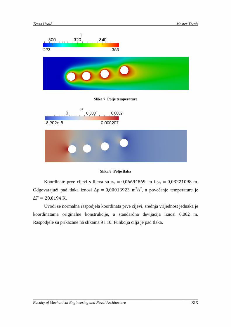
Slika 7 Polje temperature
Slika 8 Polje tlaka
Koordinate prve cijevi s lijeva su 𝑥1 = 0,06694869 m i 𝑦1 = 0,03221098 m.
Odgovarajući pad tlaka iznosi ∆𝑝 = 0,00013923 m2/s2, a povećanje temperature je
∆𝑇 = 28,0194 K.
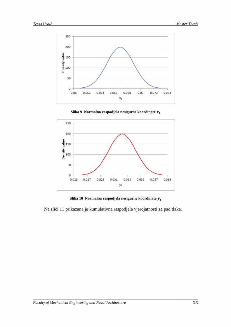
Uvodi se normalna raspodjela koordinata prve cijevi, srednja vrijednost jednaka je
koordinatama originalne konstrukcije, a standardna devijacija iznosi 0.002 m.
Raspodjele su prikazane na slikama 9 i 10. Funkcija cilja je pad tlaka.
_____________________________________________________________________________________ Faculty of Mechanical Engineering and Naval Architecture XIX
Tessa Uroić Master Thesis
Slika 9 Normalna raspodjela nesigurne koordinate 𝒙𝟏
Slika 10 Normalna raspodjela nesigurne koordinate 𝒚𝟏
Na slici 11 prikazana je kumulativna raspodjela vjerojatnosti za pad tlaka.
_____________________________________________________________________________________ Faculty of Mechanical Engineering and Naval Architecture XX
Tessa Uroić Master Thesis
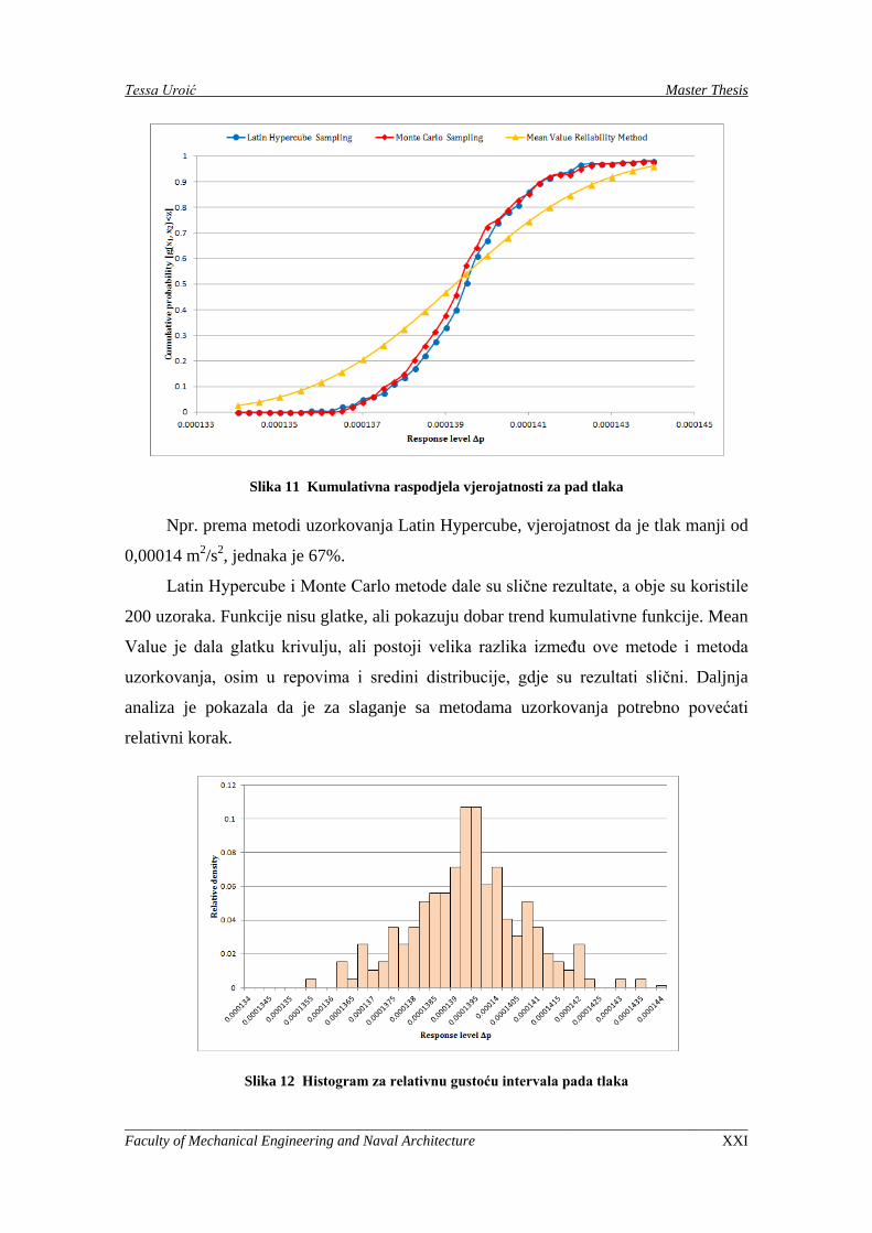
Slika 11 Kumulativna raspodjela vjerojatnosti za pad tlaka
Npr. prema metodi uzorkovanja Latin Hypercube, vjerojatnost da je tlak manji od
0,00014 m2/s2, jednaka je 67%.
Latin Hypercube i Monte Carlo metode dale su slične rezultate, a obje su koristile
200 uzoraka. Funkcije nisu glatke, ali pokazuju dobar trend kumulativne funkcije. Mean
Value je dala glatku krivulju, ali postoji velika razlika između ove metode i metoda
uzorkovanja, osim u repovima i sredini distribucije, gdje su rezultati slični. Daljnja
analiza je pokazala da je za slaganje sa metodama uzorkovanja potrebno povećati
relativni korak.
Slika 12 Histogram za relativnu gustoću intervala pada tlaka
_____________________________________________________________________________________ Faculty of Mechanical Engineering and Naval Architecture XXI

Tessa Uroić Master Thesis
Na slici 12 prikazan je histogram koji pokazuje relativnu gustoću intervala
funkcije cilja. Može se uočiti da je raspodjela približna normalnoj, ali blago nagnuta.
Izračunata srednja vrijednost jednaka je 𝜇∆𝑝 = 0,0001395 m2/s2, što je očekivano jer je
pad tlaka za originalnu konstrukciju jednak 0,00013923 m2/s2. Standardna devijacija
jednaka je 𝜎 = 0.0000017 m2/s2. Ova se konstrukcija može proglasiti relativno
stabilnom zbog uzdignute normalne raspodjele funkcije cilja (histogram, slika 12) i
relativno strme kumulativne raspodjele.
Ostale procjene i detaljni prikazi dani su u nastavku Diplomskog rada.
_____________________________________________________________________________________ Faculty of Mechanical Engineering and Naval Architecture XXII
Tessa Uroić Master Thesis
1. Introduction
In general, optimization theory is a body of mathematical results and numerical
methods for finding and identifying the best candidate from a collection of alternatives
without having to explicitly evaluate all possible alternatives [2]. To apply the
mathematical results and numerical techniques of optimization theory to concrete
engineering problems, it is necessary to define the boundaries of the engineering system
to be optimized, to define the quantitative criterion on the basis of which candidates will
be ranked to determine the best, to define a model that will express the manner in which
the variables are related.
Regardless of the performance criterion selected, in the context of optimization
the best solution will be the one with the minimum or maximum value of the
performance index. In many practical solutions, it is desirable to achieve a solution that
is the best with respect to a number of different criteria, but this is often not possible.
The following sections will provide additional information about this problem and
different approaches will be described.
Uncertainty quantification tries to determine how likely certain outcomes are if
some aspects of the system are not exactly known, [3]. Many problems in natural
sciences and engineering are associated with sources of uncertainty. For example,
parametric variability: the dimensions of a work piece in a process of manufacture may
not be exactly as designed and instructed, which would cause variability in its
performance.
Uncertainty propagation is the quantification of the uncertainties in system
output(s) propagated from the uncertain inputs. The targets of uncertainty propagation
analysis can be to evaluate low order moments of the outputs, i.e. mean value and
standard deviation, and evaluate the reliability of the outputs. The latter is especially
useful in reliability engineering where outputs of a system are usually closely related to
the performance of the system.
In the following chapters, methods for uncertainty quantification will be described
and results of the uncertainty analysis presented.
_____________________________________________________________________________________ Faculty of Mechanical Engineering and Naval Architecture 1
Tessa Uroić Master Thesis
2. Probability
Probability theory forms the basis of the assessment of probabilities of occurrence
of uncertain events and thus constitutes a cornerstone in the risk and decision analysis.
Only when a consistent basis has been established for the treatment of the uncertainties
influencing the probability that events with possible adverse consequences may occur, it
is possible to assess the risks associated with a given activity and thus to establish a
rational basis for decision making. The level of uncertainty associated with a considered
activity or phenomenon may be expressed by means of purely qualitative statements but
may also be quantified in terms of numbers or percentages.
Basics of probability theory will be introduced in this chapter, [4].
2.1. Definition of Probability
2.1.1. Frequentistic Definition
The frequentistic definition of probability is the typical interpretation of
probability by an experimentalist. In this interpretation the probability 𝑃(A) is simply
the relative frequency of occurrence of the event A as observed in an experiment with n
trials, i.e. the probability of an event A is defined as the number of times that the event
A occurs divided by the number of experiments that are carried out:
𝑃(𝐴) = 𝑙𝑖𝑚𝑁𝐴𝑛𝑒𝑥𝑝
𝑓𝑜𝑟 𝑛𝑒𝑥𝑝 → ∞ (2.1)
𝑁A is number of experiments where A occurred, 𝑛𝑒𝑥𝑝 is the total number of
experiments.
If a frequentist is asked what the probability of achieving a “head” when flipping
a coin is, he would principally not know what to answer until performing a large
number of experiments. In the mind of a frequentist, probability is a characteristic of
nature.
2.1.2. Classical Definition
The classical probability definition originates from the days when probability
calculus was founded by Pascal and Fermat. The inspiration for this theory can be found
_____________________________________________________________________________________ Faculty of Mechanical Engineering and Naval Architecture 2
Tessa Uroić Master Thesis
in games: cards or dice. The classical definition of the probability of the event A can be
formulated as:
𝑃(𝐴) =𝑛𝐴𝑛𝑡𝑜𝑡
(2.2)
where 𝑛A is the number of equally likely ways by which an experiment may lead to A,
𝑛𝑡𝑜𝑡 is the total number of equally likely ways in the experiment.
There is no real contradiction to the frequentistic definition, but the following
differences may be observed:
The experiment does not need to be carried out as the answer is known in
advance. For example, according to the classical definition of probability, the
probability of achieving a “head” when flipping a coin would be 0.5, as there is
only one possible way to achieve a “head” and there are two likely outcomes of
the experiment.
The classical theory gives no solution unless all equally possible ways can be
derived analytically.
2.1.3. Bayesian Definition
In the Bayesian interpretation the probability 𝑃(A) of the event A is formulated as
a degree of belief that A will occur:
𝑃(𝐴) = 𝑑𝑒𝑔𝑟𝑒𝑒 𝑜𝑓 𝑏𝑒𝑙𝑖𝑒𝑓 𝑡ℎ𝑎𝑡 𝐴 𝑤𝑖𝑙𝑙 𝑜𝑐𝑐𝑢𝑟 (2.3)
The degree of belief is a reflection of the state of mind of individual person in
terms of experience, expertise and preferences. The Bayesian interpretation of
probability is subjective or, more precise, person-dependant. It includes frequentistic
and classical interpretation in the sense that the subjectively assigned probabilities may
be based on experience from previous experiments (frequentistic) as well as
considerations of e.g. symmetry in coin-flipping problem (classical).
_____________________________________________________________________________________ Faculty of Mechanical Engineering and Naval Architecture 3
Tessa Uroić Master Thesis
2.2. Sample Space and Events
The set of all possible outcomes of an experiment is called the sample space
(denoted 𝛺). An event is defined as a subset of a sample space and thus a set of sample
points. If the subset is empty (i.e., contains no sample points) it is said to be impossible.
An event is said to be certain if it contains all sample points in the sample space (i.e.,
the event is identical to the sample space).
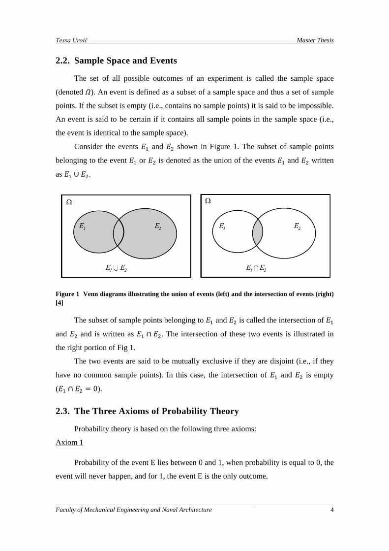
Consider the events 𝐸1 and 𝐸2 shown in Figure 1. The subset of sample points
belonging to the event 𝐸1 or 𝐸2 is denoted as the union of the events 𝐸1 and 𝐸2 written
as 𝐸1 ∪ 𝐸2.
Figure 1 Venn diagrams illustrating the union of events (left) and the intersection of events (right) [4]
The subset of sample points belonging to 𝐸1 and 𝐸2 is called the intersection of 𝐸1
and 𝐸2 and is written as 𝐸1 ∩ 𝐸2. The intersection of these two events is illustrated in
the right portion of Fig 1.
The two events are said to be mutually exclusive if they are disjoint (i.e., if they
have no common sample points). In this case, the intersection of 𝐸1 and 𝐸2 is empty
(𝐸1 ∩ 𝐸2 = 0).
2.3. The Three Axioms of Probability Theory
Probability theory is based on the following three axioms:
Axiom 1
Probability of the event E lies between 0 and 1, when probability is equal to 0, the
event will never happen, and for 1, the event E is the only outcome.
_____________________________________________________________________________________ Faculty of Mechanical Engineering and Naval Architecture 4
Tessa Uroić Master Thesis
0 ≤ 𝑃(𝐸) ≤ 1 (2.4)
for any given event 𝐸 ⊂ 𝛺 where P is the probability measure, 𝛺 is the sample space
and E is defined as a subset of a sample space.
Axiom 2
Probability of all events, i.e. probability of the entire sample space, is equal to 1.
𝑃(𝛺) = 1 (2.5)
where 𝛺 is the sample space.
Axiom 3
Given that 𝐸1,𝐸2 … is a sequence of mutually exclusive events (i.e. 𝐸1 ∩ 𝐸2 = 0
etc.) then:
𝑃 ��𝐸𝑖𝑖≥1
� = �𝑃(𝐸𝑖)𝑖≥1
(2.6)
These three axioms form the sole basis of the theory of probability.
2.4. Conditional Probability
Conditional probabilities are of special interest in risk and reliability analysis as
they form the basis of the updating of probability estimates based on new information,
knowledge and evidence.
The conditional probability of the event 𝐸1 given that the event 𝐸2 has occurred is
written as:
𝑃(𝐸1|𝐸2 �) =𝑃(𝐸1 ∩ 𝐸2)𝑃(𝐸2)
(2.7)
It is seen that the conditional probability is not defined if the conditioning event is
the empty set (𝑃(𝐸2) = 0).
The event 𝐸1 is said to be probabilistically independent of the event 𝐸2 if:
𝑃(𝐸1|𝐸2 �) = 𝑃(𝐸1) (2.8)
_____________________________________________________________________________________ Faculty of Mechanical Engineering and Naval Architecture 5
Tessa Uroić Master Thesis
implying that the occurrence of the event 𝐸2 does not affect the probability of 𝐸1. From
Eq. (2.7) the probability of the event 𝐸1 ∩ 𝐸2 may be given as:
𝑃(𝐸1 ∩ 𝐸2) = 𝑃(𝐸1|𝐸2 �)𝑃(𝐸2) (2.9)
and it follows immediately that if the events 𝐸1 and 𝐸2 are independent, then:
𝑃(𝐸1 ∩ 𝐸2) = 𝑃(𝐸1)𝑃(𝐸2) (2.10)
2.5. Characteristics of the Data
In this section, the numerical characteristics of the observed data containing
important information about the data and the nature of uncertainty associated with these.
These are also referred to as sample characteristics. Descriptive statistics play an
important role in engineering as a standardized basis for assessing and documenting
data obtained for the purpose of understanding and representing uncertainties.
2.5.1. Central Measures
One of the most useful numerical summaries is the sample mean. If the data set is
collected in the vector 𝑥 = (𝑥1, 𝑥2, … , 𝑥𝑛) the sample mean �̅� is simply given as:
�̅� =1𝑛�𝑥𝑖
𝑛
𝑖=1
(2.11)
The sample mean may be interpreted as a central value of the data set. if, on the basis of
the data set, one should give only one value characterizing the data, the sample mean
would normally be used.
Another central measure is the mode of the data set, i.e. the most frequently
occurring value in the data set. When data samples are real values, the mode in general
cannot be assessed numerically, but may be assessed from graphical representations of
the data.
It is often convenient to work with an ordered data set which is readily established
by rearranging the original data set 𝑥 = (𝑥1, 𝑥2, … , 𝑥𝑛) such that the data are arranged in
increasing order as 𝑥1𝑂 ≤ 𝑥2𝑂 ≤ ⋯ ≤ 𝑥𝑖𝑂 ≤ ⋯ ≤ 𝑥𝑛−1𝑂 ≤ 𝑥𝑛𝑂.
_____________________________________________________________________________________ Faculty of Mechanical Engineering and Naval Architecture 6
Tessa Uroić Master Thesis
The median of the data set is defined as the middle value in the ordered list of data
if n is odd. If n is even, the median is taken as the average value of the two middle
values.
2.5.2. Dispersion Measures
The variability or the dispersion of the data set around the sample mean is also an
important characteristic of the data set. The dispersion may be characterized by the
sample variance 𝑠2 given by:
𝑠2 =1𝑛�(𝑥𝑖 − �̅�)2𝑛
𝑖=1
(2.12)
The sample standard deviation s is defined as the square root of the sample variance.
From Eq. (2.12) it is seen that the sample standard deviation is assessed in terms of the
variability of the observations around the sample mean value �̅�.
2.5.3. Other Measures
Whereas the sample mean, mode and median are central measures of a data set
and the sample variance is a measure of the dispersion around the sample mean, it is
also useful to have some characteristics indicating the degree of symmetry of the data
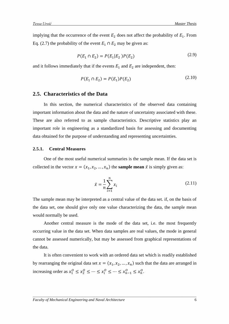
set. To this end, the sample coefficient of skewness (Figure 2), which is a simple
logical extension of the sample variance is suitable. The sample coefficient of skewness
η is defined as:
η =1𝑛∑ (𝑥𝑖 − �̅�)3𝑛𝑖=1
𝑠3 (2.13)
This coefficient is positive if the mode of the data set is less than its mean value
(skewed to the right) and negative if the mode is larger than the mean value (skewed to
the left).
_____________________________________________________________________________________ Faculty of Mechanical Engineering and Naval Architecture 7
Tessa Uroić Master Thesis
Figure 2 Illustration of skewness
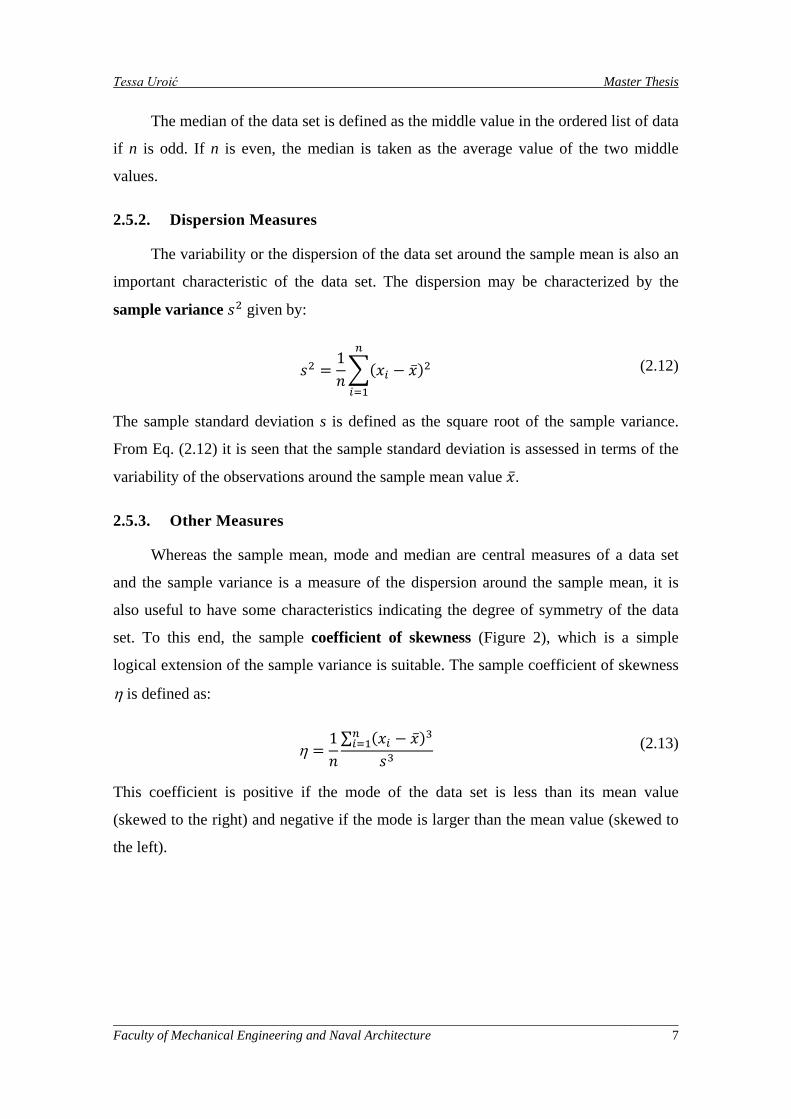
In a similar way, the sample coefficient of kurtosis κ (Figure 3) is defined as:
κ =1𝑛∑ (𝑥𝑖 − �̅�)4𝑛𝑖=1
𝑠4 (2.14)
which is a measure of how closely the data are distributed around the mode
(peakedness).
Figure 3 Illustration of kurtosis
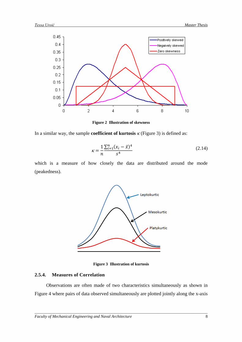
2.5.4. Measures of Correlation
Observations are often made of two characteristics simultaneously as shown in
Figure 4 where pairs of data observed simultaneously are plotted jointly along the x-axis
_____________________________________________________________________________________ Faculty of Mechanical Engineering and Naval Architecture 8
Tessa Uroić Master Thesis
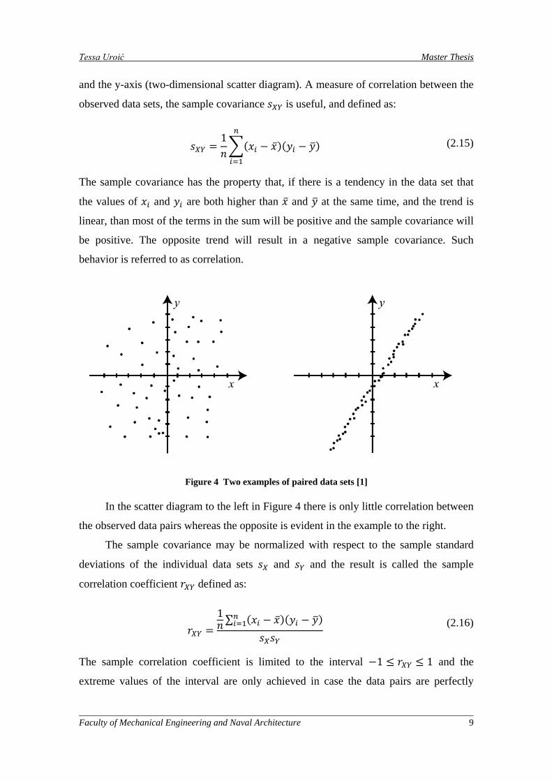
and the y-axis (two-dimensional scatter diagram). A measure of correlation between the
observed data sets, the sample covariance 𝑠𝑋𝑌 is useful, and defined as:
𝑠𝑋𝑌 =1𝑛�(𝑥𝑖 − �̅�)(𝑦𝑖 − 𝑦�)𝑛
𝑖=1
(2.15)
The sample covariance has the property that, if there is a tendency in the data set that
the values of 𝑥𝑖 and 𝑦𝑖 are both higher than �̅� and 𝑦� at the same time, and the trend is
linear, than most of the terms in the sum will be positive and the sample covariance will
be positive. The opposite trend will result in a negative sample covariance. Such
behavior is referred to as correlation.
Figure 4 Two examples of paired data sets [1]
In the scatter diagram to the left in Figure 4 there is only little correlation between
the observed data pairs whereas the opposite is evident in the example to the right.
The sample covariance may be normalized with respect to the sample standard
deviations of the individual data sets 𝑠𝑋 and 𝑠𝑌 and the result is called the sample
correlation coefficient 𝑟𝑋𝑌 defined as:
𝑟𝑋𝑌 =1𝑛∑ (𝑥𝑖 − �̅�)(𝑦𝑖 − 𝑦�)𝑛
𝑖=1
𝑠𝑋𝑠𝑌
(2.16)
The sample correlation coefficient is limited to the interval −1 ≤ 𝑟𝑋𝑌 ≤ 1 and the
extreme values of the interval are only achieved in case the data pairs are perfectly
_____________________________________________________________________________________ Faculty of Mechanical Engineering and Naval Architecture 9
Tessa Uroić Master Thesis
correlated, implying that the points on the scatter diagram lie on a straight line. For the
example shown in Fig. 4 there is almost zero correlation at the left hand side and almost
full positive correlation on the right hand side.
2.6. Uncertainty Modeling
For the purpose of discussing the phenomenon uncertainty in more detail, it is
assumed that the universe is deterministic and that the knowledge about the universe is
perfect. This implies that it is possible to achieve perfect knowledge about any state,
quantity or characteristic, by means of e.g. a set of exact equation systems and known
boundary conditions. It would be possible to gain knowledge about phenomena which
cannot be directly observed or have not taken place yet. In principle, following this line
of reasoning, the future as well as the past would be known or assessable with certainty.
Whether the universe is deterministic or not is a rather deep philosophical and
physical question. Despite the obviously challenging aspects of this question its answer
is, however, not a prerequisite for purposes of engineering decision making because
even if the universe is deterministic, our knowledge about it is still in part incomplete
and/or uncertain.
It has become standard to differentiate between uncertainties due to inherent
natural variability, model uncertainties and statistical uncertainties. The first mentioned
type of uncertainty is often denoted as aleatory uncertainty and the two latter types are
referred to as epistemic uncertainties.
2.6.1. Random Variables
The performance of an engineered system, facility or installation may usually be
modeled in mathematical and physical terms in conjunction with empirical relations.
For a given set of model parameters the performance of the considered system can
be determined on the basis of this model. The basic random variables are defined as the
parameter that represents the available knowledge as well as the associated uncertainty
in the considered model.
The basic random variables must be able to represent all types of uncertainties
that are included in the analysis. The uncertainties which must be considered are
physical uncertainty, statistical uncertainty and the model uncertainty. The physical
uncertainties are typically uncertainties associated with the environment, the geometry _____________________________________________________________________________________ Faculty of Mechanical Engineering and Naval Architecture 10
Tessa Uroić Master Thesis
of the structure and the material properties. The statistical uncertainties arise due to
incomplete statistical information e.g. due to a small number of material tests. Finally,
the model uncertainties must be considered to take into account the uncertainty
associated with the idealized mathematical descriptions used to approximate the actual
physical behavior of the structure.
Modern methods of reliability and risk analysis allow for a very general
representation of these uncertainties ranging from non-stationary stochastic processes
and fields to time invariant random variables. In most cases, it is sufficient to model the
uncertain quantities by random variables with given cumulative distribution functions
and distribution parameters estimated on basis of statistical and/or subjective
information. Therefore, the following is concerned with a basic description of the
characteristics of random variables.
Cumulative Distribution and Probability Density Functions
A random variable, which can take any real value, is called a continuous random
variable. The probability that such random variable takes a specific value is zero, as
there is an infinite number of values in real space. The probability that a continuous
random variable, X, is less than or equal to a value, x, is given by the cumulative
distribution function:
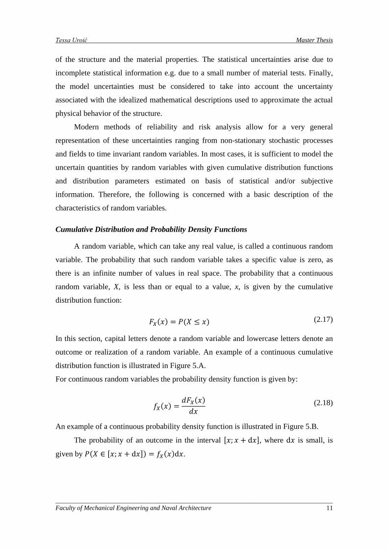
𝐹𝑋(𝑥) = 𝑃(𝑋 ≤ 𝑥) (2.17)
In this section, capital letters denote a random variable and lowercase letters denote an
outcome or realization of a random variable. An example of a continuous cumulative
distribution function is illustrated in Figure 5.A.
For continuous random variables the probability density function is given by:
𝑓𝑋(𝑥) =𝑑𝐹𝑋(𝑥)𝑑𝑥
(2.18)
An example of a continuous probability density function is illustrated in Figure 5.B.
The probability of an outcome in the interval [𝑥; 𝑥 + d𝑥], where d𝑥 is small, is
given by 𝑃(𝑋 ∈ [𝑥; 𝑥 + d𝑥]) = 𝑓𝑋(𝑥)d𝑥.
_____________________________________________________________________________________ Faculty of Mechanical Engineering and Naval Architecture 11
Tessa Uroić Master Thesis
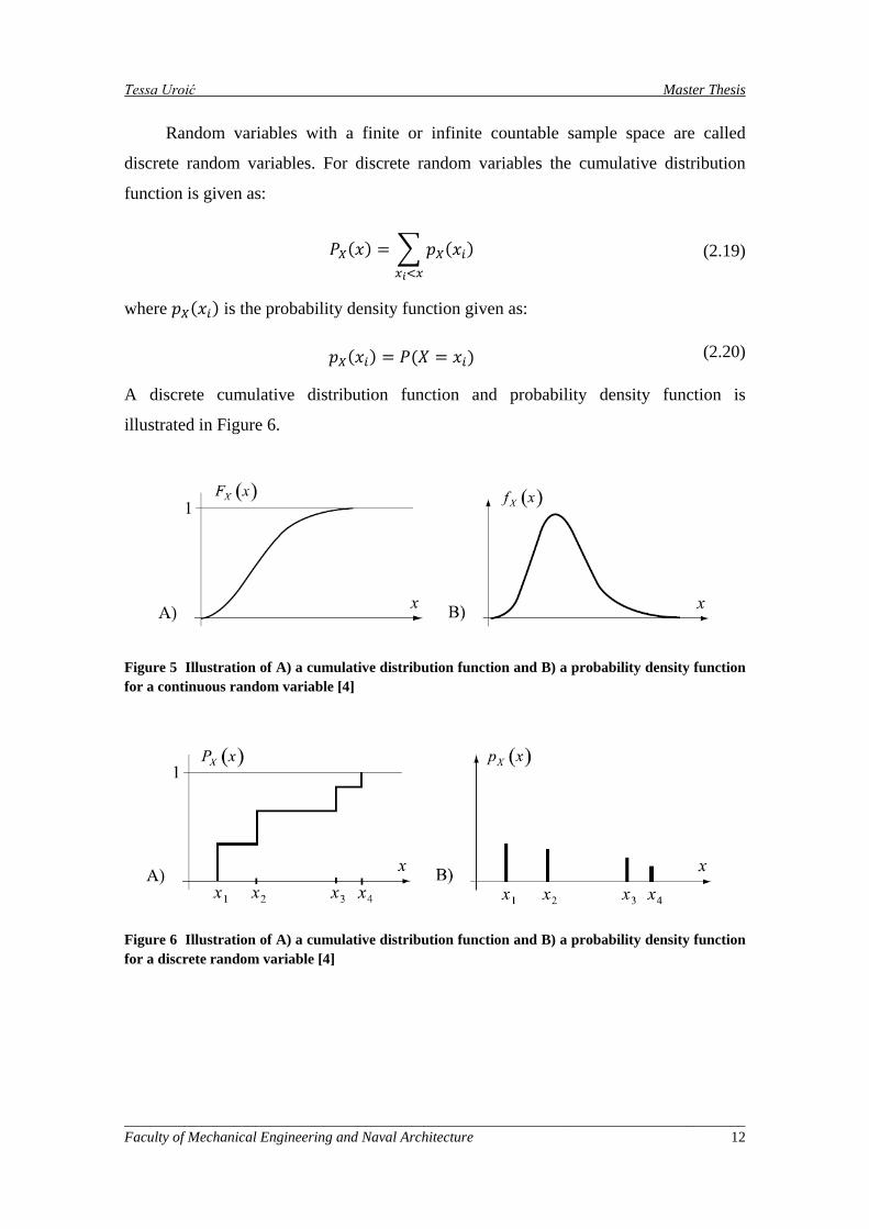
Random variables with a finite or infinite countable sample space are called
discrete random variables. For discrete random variables the cumulative distribution
function is given as:
𝑃𝑋(𝑥) = � 𝑝𝑋(𝑥𝑖)𝑥𝑖<𝑥
(2.19)
where 𝑝𝑋(𝑥𝑖) is the probability density function given as:
𝑝𝑋(𝑥𝑖) = 𝑃(𝑋 = 𝑥𝑖) (2.20)
A discrete cumulative distribution function and probability density function is
illustrated in Figure 6.
Figure 5 Illustration of A) a cumulative distribution function and B) a probability density function for a continuous random variable [4]
Figure 6 Illustration of A) a cumulative distribution function and B) a probability density function for a discrete random variable [4]
_____________________________________________________________________________________ Faculty of Mechanical Engineering and Naval Architecture 12
Tessa Uroić Master Thesis
Moments of Continuous Random Variable and the Expectation Operator
Probability distributions may be defined in terms of their parameters or moments.
Often cumulative distribution functions and probability density functions are written as
𝐹𝑋(𝑥;𝑝) and 𝑓𝑋(𝑥;𝑝) respectively to indicate the parameters p (or moments) defining
the functions. Whether the cumulative distribution and density function are defined by
their moments or by their parameters is a matter of convenience and it is generally
possible to establish one from another.
The ith moment λ𝑖 of a continuous random variable is defined by:
λ𝑖 = � 𝑥𝑖∞
−∞
𝑓𝑋(𝑥)𝑑𝑥 (2.21)
The mean (or expected value) of a continuous random variable X is defined as the first
moment:
𝜇𝑋 = 𝐸[𝑋] = � 𝑥∞
−∞
𝑓𝑋(𝑥)𝑑𝑥 (2.22)
where 𝐸[ ] is the expectation operation. Its linearity property is useful since it can be
used, for example, to find the following formula for variance of a random variable X in
terms of more easily calculated quantities:
𝜎𝑋2 = 𝐸[(𝑋 − 𝜇𝑥)2] = 𝐸[(𝑋2 − 2𝜇𝑋 ∙ 𝑋 + 𝜇𝑋2)]= 𝜇𝑋2 + 𝐸[𝑋2] − 2𝜇𝑋 ∙ 𝐸[𝑋] == 𝜇𝑋2 + 𝐸[𝑋2] − 2𝜇𝑋2= 𝐸[𝑋2] − 𝜇𝑋2 (2.23)
The variance 𝜎𝑋2, is described by the second central moment, i.e. for continuous random
variables it is:
𝜎𝑋2 = 𝑉𝑎𝑟[𝑋] = 𝐸[(𝑋 − 𝜇𝑋)2] = �(𝑥 − 𝜇𝑋)2∞
−∞
𝑓𝑋(𝑥)𝑑𝑥 (2.24)
where 𝑉𝑎𝑟[𝑋] denotes the variance of X.
The ratio between the standard deviation 𝜎𝑋 and the expected value 𝜇𝑋 of a
random variable X is denoted the coefficient of variation 𝑉𝑋 and is given by:
_____________________________________________________________________________________ Faculty of Mechanical Engineering and Naval Architecture 13
Tessa Uroić Master Thesis
𝑉𝑋 =𝜎𝑋 𝜇𝑋
(2.25)
The coefficient of variation provides a useful descriptor for the variability of a
random variable around its expected value.
The Probability Distribution for Functions of Random Variables
In some cases it is interesting to be able to derive the cumulative distribution
function 𝐹𝑌(𝑦) for a random variable 𝑌 which is given as a function of another random
variable X, i.e. 𝑌 = 𝑔(𝑋), with given cumulative distribution function 𝐹𝑋(𝑥). Under the
condition that the function 𝑔(𝑋) is monotonically increasing and furthermore,
represents a one-to-one mapping of 𝑥 into 𝑦, a realization of 𝑌 is only smaller than 𝑦0 if
correspondingly the realization of 𝑋 is smaller than 𝑥0 which in turn is given by
𝑥0 = 𝑔−1(𝑦0). In this case the cumulative distribution function 𝐹𝑌(𝑦) can be readily
determined by:
𝐹𝑌(𝑦) = 𝑃(𝑌 ≤ 𝑦) = 𝑃(𝑋 ≤ 𝑔−1(𝑦)) (2.26)
which is also written as:
𝐹𝑌(𝑦) = 𝑃(𝑌 ≤ 𝑦) = 𝑃(𝑋 ≤ 𝑔−1(𝑦)) (2.27)
𝐹𝑌(𝑦) = 𝐹𝑋(𝑔−1(𝑦)) (2.28)
The probability density function 𝑓𝑌(𝑦) is simply given by:
𝑓𝑌(𝑦) =𝑑𝐹𝑋(𝑔−1(𝑦))
𝑑𝑦 (2.29)
which immediately leads to:
𝑓𝑌(𝑦) =𝑑𝑔−1(𝑦)𝑑𝑦
𝑓𝑋(𝑔−1(𝑦)) (2.30)
and:
𝑓𝑌(𝑦) =𝑑𝑥𝑑𝑦
𝑓𝑋(𝑥) (2.31)
_____________________________________________________________________________________ Faculty of Mechanical Engineering and Naval Architecture 14
Tessa Uroić Master Thesis
It is noticed that the application of Equations (2.30) and (2.31) necessitates that 𝑔(𝑥) is
at least one time differentiable in regard to x.
If the function 𝑔(𝑥) instead of being monotonically increasing is monotonically
decreasing, a realization of 𝑌 smaller than 𝑦0 corresponds to a realization of X larger
than 𝑥0, in which case it is necessary to change the sign of the derivative d𝑥d𝑦
in Eq.
(2.31). Generally, for monotonically increasing or decreasing one-to-one functions 𝑔(𝑥)
there is:
𝑓𝑌(𝑦) = �𝑑𝑥𝑑𝑦� 𝑓𝑋(𝑥) (2.32)
Consider the random vector 𝑌 = (𝑌1,𝑌2, … ,𝑌𝑛)𝑇 with individual components given as
one-to-one mapping monotonically increasing or decreasing functions 𝑔𝑖, 𝑖 = 1,2, … ,𝑛
of the components of the random vector 𝑋 = (𝑋1,𝑋2, … ,𝑋𝑛)𝑇 as:
𝑌𝑖 = 𝑔𝑖(𝑋) (2.33)
then there is:
𝑓𝑌(𝑦) = |𝐽|𝑓𝑋(𝑥) (2.34)
where |𝐽| is the numerical value of the determinant of 𝐽 given by:
|𝐽| =
⎣⎢⎢⎢⎡𝑑𝑥1𝑑𝑦1
⋯𝑑𝑥1𝑑𝑦𝑛
⋮ ⋱ ⋮𝑑𝑥𝑛𝑑𝑦1
⋯𝑑𝑥𝑛𝑑𝑦𝑛⎦
⎥⎥⎥⎤
(2.35)
Finally, the expected value 𝐸[𝑌] of a function 𝑔(𝑥) of the random vector 𝑋 =
(𝑋1,𝑋2, … ,𝑋𝑛)𝑇 is given by:
𝐸[𝑌] = � ⋯ � 𝑔(𝑥)∞
−∞
∞
−∞
𝑓𝑋(𝑥)𝑑𝑥1 …𝑑𝑥𝑛 (2.36)
_____________________________________________________________________________________ Faculty of Mechanical Engineering and Naval Architecture 15
Tessa Uroić Master Thesis
The Central Limit Theorem and Derived Distributions
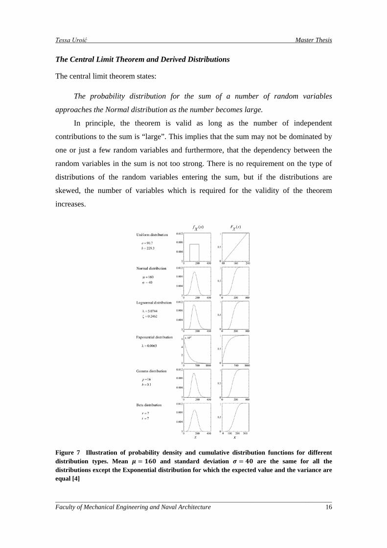
The central limit theorem states:
The probability distribution for the sum of a number of random variables
approaches the Normal distribution as the number becomes large.
In principle, the theorem is valid as long as the number of independent
contributions to the sum is “large”. This implies that the sum may not be dominated by
one or just a few random variables and furthermore, that the dependency between the
random variables in the sum is not too strong. There is no requirement on the type of
distributions of the random variables entering the sum, but if the distributions are
skewed, the number of variables which is required for the validity of the theorem
increases.
Figure 7 Illustration of probability density and cumulative distribution functions for different distribution types. Mean 𝝁 = 𝟏𝟔𝟎 and standard deviation 𝝈 = 𝟒𝟎 are the same for all the distributions except the Exponential distribution for which the expected value and the variance are equal [4]
_____________________________________________________________________________________ Faculty of Mechanical Engineering and Naval Architecture 16
Tessa Uroić Master Thesis
The Normal Distribution
The significant practical importance of the central limit theorem lies in the fact
that even though only weak information is available regarding the number of
contributions and their joint probability density function, rather strong information is
achieved for the distribution of sum of the contributions.
The Normal probability distribution is thus applied very frequently in practical
problems for the probabilistic modeling of uncertain phenomena which may be
considered to originate from a cumulative effect of several independent uncertain
contributions.
The Normal distribution has the property that the linear combination 𝑆 of 𝑛
Normal distributed random variable 𝑋𝑖 , 𝑖 = 1,2, … ,𝑛:
𝑆 = 𝑎0 + �𝑎𝑖𝑋𝑖
𝑛
𝑖=1
(2.37)
is also Normal distributed. The distribution is said to be closed in respect to summation.
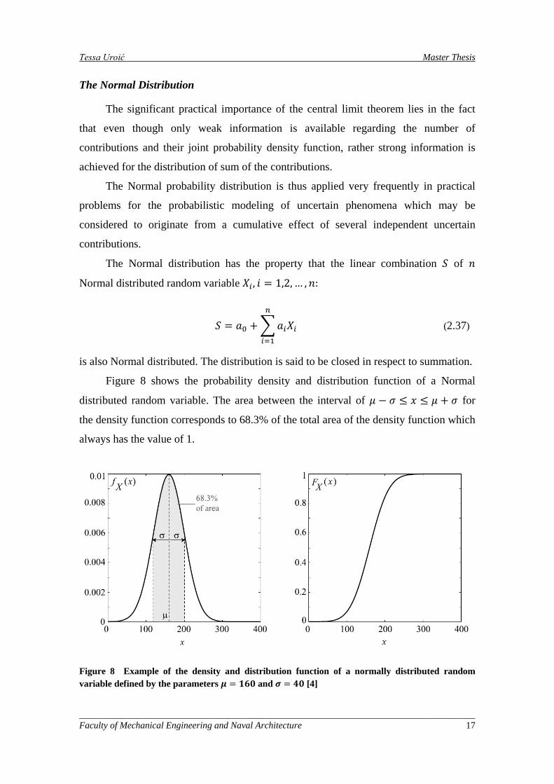
Figure 8 shows the probability density and distribution function of a Normal
distributed random variable. The area between the interval of 𝜇 − 𝜎 ≤ 𝑥 ≤ 𝜇 + 𝜎 for
the density function corresponds to 68.3% of the total area of the density function which
always has the value of 1.
Figure 8 Example of the density and distribution function of a normally distributed random variable defined by the parameters 𝝁 = 𝟏𝟔𝟎 and 𝝈 = 𝟒𝟎 [4]
_____________________________________________________________________________________ Faculty of Mechanical Engineering and Naval Architecture 17
Tessa Uroić Master Thesis
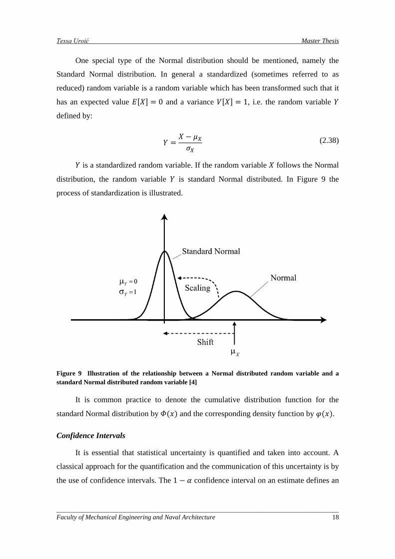
One special type of the Normal distribution should be mentioned, namely the
Standard Normal distribution. In general a standardized (sometimes referred to as
reduced) random variable is a random variable which has been transformed such that it
has an expected value 𝐸[𝑋] = 0 and a variance 𝑉[𝑋] = 1, i.e. the random variable 𝑌
defined by:
𝑌 =𝑋 − 𝜇𝑋𝜎𝑋
(2.38)
𝑌 is a standardized random variable. If the random variable 𝑋 follows the Normal
distribution, the random variable 𝑌 is standard Normal distributed. In Figure 9 the
process of standardization is illustrated.
Figure 9 Illustration of the relationship between a Normal distributed random variable and a standard Normal distributed random variable [4]
It is common practice to denote the cumulative distribution function for the
standard Normal distribution by 𝛷(𝑥) and the corresponding density function by 𝜑(𝑥).
Confidence Intervals
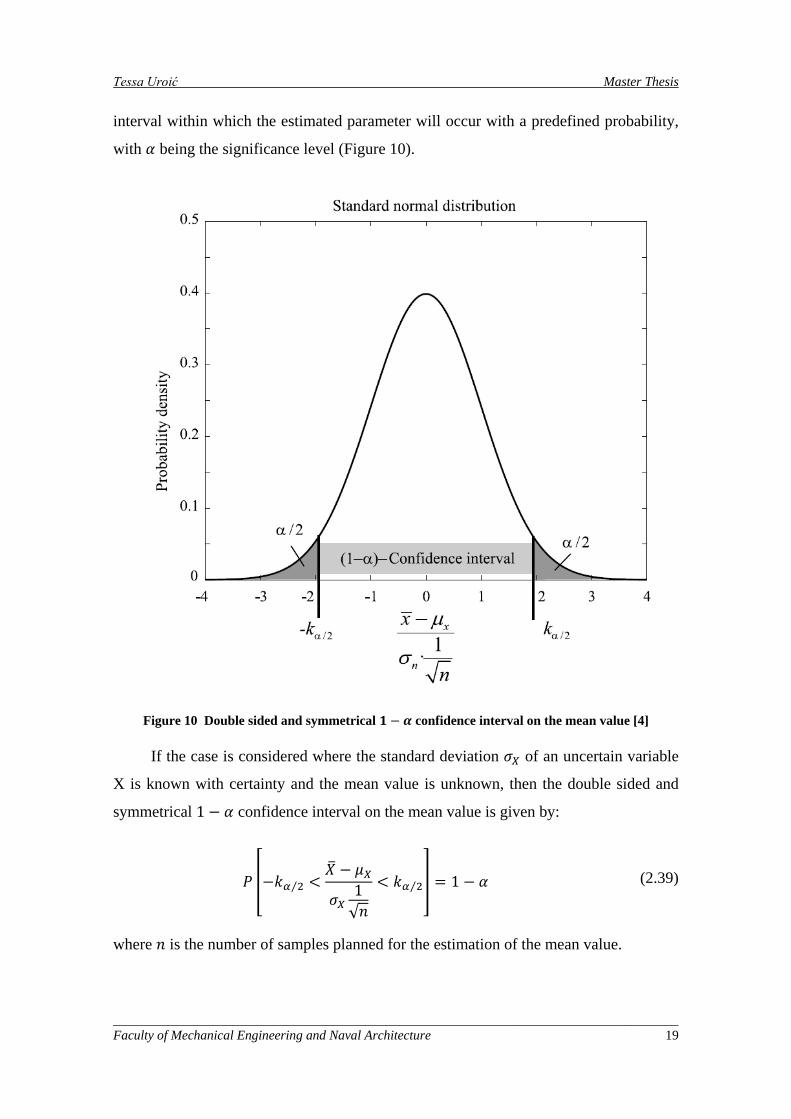
It is essential that statistical uncertainty is quantified and taken into account. A
classical approach for the quantification and the communication of this uncertainty is by
the use of confidence intervals. The 1 − 𝛼 confidence interval on an estimate defines an
_____________________________________________________________________________________ Faculty of Mechanical Engineering and Naval Architecture 18
Tessa Uroić Master Thesis
interval within which the estimated parameter will occur with a predefined probability,
with 𝛼 being the significance level (Figure 10).
Figure 10 Double sided and symmetrical 𝟏 − 𝜶 confidence interval on the mean value [4]
If the case is considered where the standard deviation 𝜎𝑋 of an uncertain variable
X is known with certainty and the mean value is unknown, then the double sided and
symmetrical 1 − 𝛼 confidence interval on the mean value is given by:
𝑃 �−𝑘𝛼 2⁄ <𝑋� − 𝜇𝑋
𝜎𝑋1√𝑛
< 𝑘𝛼 2⁄ � = 1 − 𝛼 (2.39)
where 𝑛 is the number of samples planned for the estimation of the mean value.
_____________________________________________________________________________________ Faculty of Mechanical Engineering and Naval Architecture 19
Tessa Uroić Master Thesis
From Eq. (2.39) it is seen that the confidence interval limits depend on 𝛼, 𝑛 and
𝜎𝑋. Typically 𝛼 is chosen as 0.1, 0.05 and 0.01 in engineering applications. Narrow
confidence intervals may be achieved by increasing the number of experiments, which
on the other hand, may be expensive to achieve and in some cases not even possible for
practical reasons.
2.7. Methods of Reliability
2.7.1. Failure Events and Basic Random Variables
In reliability analysis of technical systems and components the main problem is to
evaluate the probability of failure corresponding to a specified reference period.
However, other non-failure states of the considered component or system may also be
of interest, such as excessive damage, unavailability, etc.
In general, any state which may be associated with consequences in terms of
costs, loss of lives and impact to the environment is of interest. In the following section
no differentiation will be made between these different types of states. For simplicity,
all these events will be referred to as being failure events, bearing in mind, however,
that also non-failure states may be considered in the same manner.
It is convenient to describe failure events in terms of functional relations. If they
are fulfilled, the considered event will occur. A failure event may be described by a
functional relation, the limit state function 𝑔(𝑥), in the following way:
𝐹 = {𝑔(𝑥) ≤ 0} (2.40)
where the components of the vector 𝑥 are realizations of the basic random variables 𝑋
representing all the relevant uncertainties influencing the probability of failure. In Eq.
(2.40) the failure event 𝐹 is simply defined as the set of realizations of the function
𝑔(𝑥), which is zero or negative.
Having defined the failure event, the probability of failure 𝑃𝐹 may be determined
by the following integral:
𝑃𝐹 = � 𝑓𝑋(𝑥)𝑑𝑥𝑔(𝑥)≤0
(2.41)
_____________________________________________________________________________________ Faculty of Mechanical Engineering and Naval Architecture 20
Tessa Uroić Master Thesis
where 𝑓𝑋(𝑥) is the joint probability density function of the random variables 𝑋. This
integral is, however, non-trivial to solve and numerical approximations are expedient.
Various methods for the solution of the integral in Eq. (2.41) have been proposed
including numerical integration techniques, Monte Carlo simulations and asymptotic
Laplace expansions. Numerical integration techniques very rapidly become inefficient
for increasing size of the vector 𝑋. In the following section the focus is directed toward
the widely applied and quite efficient First Order Reliability Methods (FORM) [8],
which furthermore are consistent with the solutions obtained by asymptotic Laplace
integral expansions.
2.7.2. Linear Limit State Functions and Normal Distributed Variables
For illustrative purposes first the case where the limit state function 𝑔(𝑥) is linear
function of the basic random variables 𝑋 is considered. Then the limit state function
may be written as:
𝑔(𝑥) = 𝑎0 + �𝑎𝑖𝑥𝑖
𝑛
𝑖=1
(2.42)
The safety margin is then defined as 𝑀 = 𝑔(𝑥). Failure can be defined by:
𝑀 ≤ 0 (2.43)
If the basic random variables are Normal distributed, the linear safety margin M defined
through:
𝑀 = 𝑎0 + �𝑎𝑖𝑋𝑖
𝑛
𝑖=1
(2.44)
is also Normal distributed with mean value and variance:
𝜇𝑀 = 𝑎0 + �𝑎𝑖𝜇𝑋𝑖
𝑛
𝑖=1
(2.45)
_____________________________________________________________________________________ Faculty of Mechanical Engineering and Naval Architecture 21
Tessa Uroić Master Thesis
𝜎𝑀2 = �𝑎𝑖2𝜎𝑋𝑖2
𝑛
𝑖=1
+ 2�� � 𝑎𝑖𝑎𝑗𝐶𝑋𝑖𝑋𝑗
𝑛
𝑗=𝑖+1
𝑛
𝑖=1
�
= �𝑎𝑖2𝜎𝑋𝑖2
𝑛
𝑖=1
+ 2�� � 𝑎𝑖𝑎𝑗𝜌𝑖𝑗𝜎𝑋𝑖𝜎𝑋𝑗
𝑛
𝑗=𝑖+1
𝑛
𝑖=1
�
(2.46)
𝜌𝑖𝑗 are the correlation coefficients between the variables 𝑋𝑖 and 𝑋𝑗.
Defining the failure event by Eq. (2.40), the probability of failure can be written as:
𝑃𝐹 = 𝑃(𝑔(𝑥) ≤ 0) = 𝑃(𝑀 ≤ 0) (2.47)
which in this simple case reduces to the evaluation of the standard Normal distribution
function:
𝑃𝐹 = 𝛷 �0 − 𝜇𝑀𝜎𝑀
� = 𝛷(−𝛽) (2.48)
where the reliability index 𝛽 is given as:
𝛽 =𝜇𝑀𝜎𝑀
(2.49)
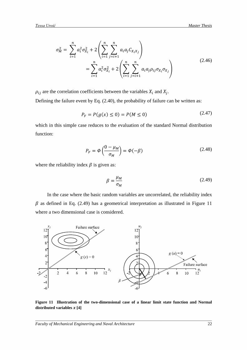
In the case where the basic random variables are uncorrelated, the reliability index
𝛽 as defined in Eq. (2.49) has a geometrical interpretation as illustrated in Figure 11
where a two dimensional case is considered.
Figure 11 Illustration of the two-dimensional case of a linear limit state function and Normal distributed variables 𝒙 [4]
_____________________________________________________________________________________ Faculty of Mechanical Engineering and Naval Architecture 22
Tessa Uroić Master Thesis
In Figure 11 the limit state function 𝑔(𝑥) has been transformed into the limit state
function 𝑔(𝑢) by standardization of the random variables as:
𝑈𝑖 =𝑋𝑖 − 𝜇𝑋𝑖𝜎𝑋𝑖
(2.50)
such that the random variables 𝑈𝑖 have mean values equal to zero and standard
deviation values equal to one.
The reliability index 𝛽 has the simple geometrical interpretation as the smallest
distance from the line (or generally the hyper-plane) forming the boundary between the
safe domain and the failure domain, i.e. the domain defined by the failure event. It
should be noted that this definition of the reliability index does not depend on the limit
state function but rather the boundary between the safe domain and the failure domain.
The point on the failure surface with the smallest distance to the origin is commonly
called the design point or the most likely failure point.
It is seen that the evaluation of the probability of failure in this simple case
reduces to a simple evaluation in terms of mean values and standard deviations of the
basic random variables, i.e. the first and second order information.
2.7.3. The Error Propagation Law
The results given in Eq.(2.45) and (2.46) have been applied to study the statistical
characteristics of errors 𝜀 accumulating in accordance with some differentiable function
ℎ(𝑥), i.e.
𝜀 = ℎ(𝑥) (2.51)
where 𝑥 = 𝑥1, 𝑥2, … , 𝑥𝑛 is a vector of realizations of the basic random variables X
representing measurement uncertainties with mean values 𝜇𝑋 = 𝜇𝑋1 , 𝜇𝑋2 , … , 𝜇𝑋𝑛 and
covariances 𝐶𝑋𝑖𝑋𝑗 = 𝜌𝑖𝑗𝜎𝑋𝑖𝜎𝑋𝑗 where 𝜎𝑋𝑖 are standard deviations and 𝜌𝑖𝑗 are the
correlation coefficients. The idea is to approximate the function ℎ(𝑥) by its Taylor
expansion including only the linear terms, i.e.:
𝜀 ≅ ℎ(𝑥0) + ��𝑥𝑖 − 𝑥𝑖,0�𝑛
𝑖=1
�𝜕ℎ(𝑥)𝜕𝑥𝑖
�𝑥=𝑥0
(2.52)
_____________________________________________________________________________________ Faculty of Mechanical Engineering and Naval Architecture 23
Tessa Uroić Master Thesis
where 𝑥0 = 𝑥1,0, 𝑥2,0, … , 𝑥𝑛,0 is the point in which the linearization is performed,
normally chosen as the mean value point.
�𝜕ℎ(𝑥)𝜕𝑥𝑖
�𝑥=𝑥0
, 𝑖 = 1,2, … ,𝑛 are the first order partial derivatives of ℎ(𝑥) taken in
𝑥 = 𝑥0. From Equations (2.52), (2.45) and (2.46) it is seen that the expected value of
the error 𝐸[𝜀] can be assessed by:
𝐸[𝜀] ≅ ℎ(𝜇𝑋) (2.53)
and its variance 𝑉𝑎𝑟[𝜀] can be determined by:
𝑉𝑎𝑟[𝜀] ≅���𝜕ℎ(𝑥)𝜕𝑥𝑖
�𝑥=𝑥0
�2𝑛
𝑖=1
𝜎𝑋𝑖2
+ 2� � ��𝜕ℎ(𝑥)𝜕𝑥𝑖
�𝑥=𝑥0
�𝑛
𝑗=𝑖+1
𝑛
𝑖=1
��𝜕ℎ(𝑥)𝜕𝑥𝑖
�𝑥=𝑥0
� 𝜌𝑖𝑗𝜎𝑋𝑖𝜎𝑋𝑗 (2.54)
It is important to notice that the variance of the error as given by Eq. (2.54) depends on
the linearization point, i.e. 𝑥0 = 𝑥1,0, 𝑥2,0, … , 𝑥𝑛,0.
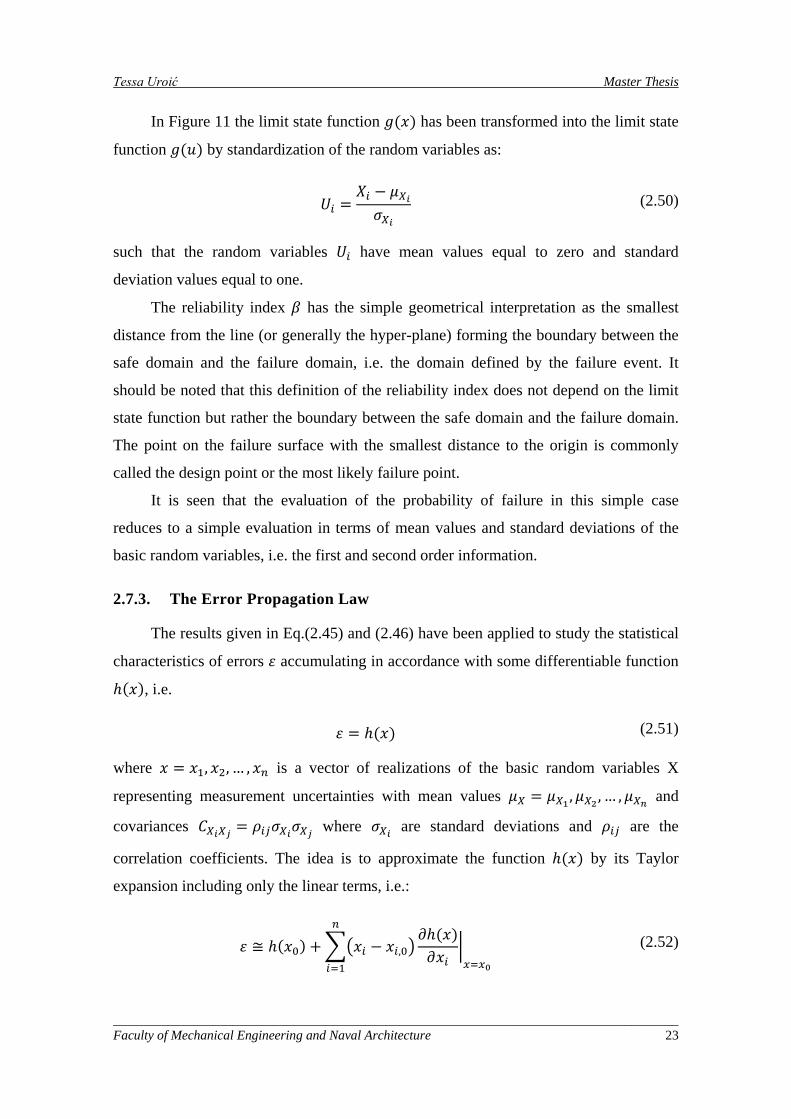
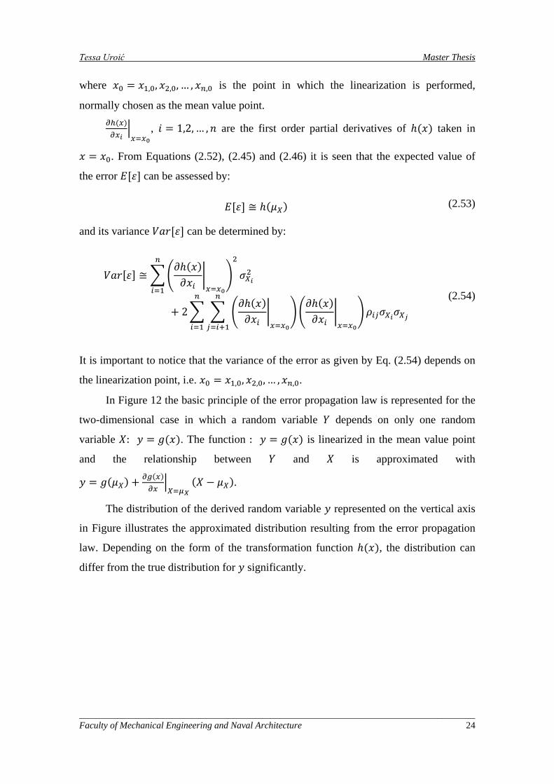
In Figure 12 the basic principle of the error propagation law is represented for the
two-dimensional case in which a random variable 𝑌 depends on only one random
variable 𝑋: 𝑦 = 𝑔(𝑥). The function : 𝑦 = 𝑔(𝑥) is linearized in the mean value point
and the relationship between 𝑌 and 𝑋 is approximated with
𝑦 = 𝑔(𝜇𝑋) + �𝜕𝑔(𝑥)𝜕𝑥
�𝑋=𝜇𝑋
(𝑋 − 𝜇𝑋).
The distribution of the derived random variable 𝑦 represented on the vertical axis
in Figure illustrates the approximated distribution resulting from the error propagation
law. Depending on the form of the transformation function ℎ(𝑥), the distribution can
differ from the true distribution for 𝑦 significantly.
_____________________________________________________________________________________ Faculty of Mechanical Engineering and Naval Architecture 24
Tessa Uroić Master Thesis
Figure 12 Illustration of the error propagation law: The transformation of the density function 𝒇𝒀(𝒚) according to the relation 𝒚 = 𝒈(𝒙) and the linear approximation of the relation between the two random variables [4]
2.7.4. Non-linear Limit State Functions
When the limit state function is non-linear in the basic random variables X, the
situation is not as simple as outlined in the previous section. An obvious approach is,
however, to consider the error propagation law to represent the failure domain in terms
of a linearization of the boundary between the safe domain and the failure domain, i.e.
the failure surface. Still, the question remains how to do this appropriately.
Hasofer and Lind [5] suggest to perform this linearization in the design point of
the failure surface in normalized space. The situation is illustrated in the 2-dimesional
space in Fig 13.
A principal sketch is given, illustrating that the failure surface is linearized in the
design point 𝑢∗ by the line 𝑔′(𝑢) = 0. The 𝛼-vector is the outward directed normal
vector to the failure surface with the shortest distance 𝛽 to the origin.
_____________________________________________________________________________________ Faculty of Mechanical Engineering and Naval Architecture 25
Tessa Uroić Master Thesis
As the limit state function is in general non-linear, one does not know the design
point in advance. This has to be found, e.g. by solving the following optimization
problem:
𝛽 = 𝑚𝑖𝑛𝑢𝜖{𝑔(𝑢)=0}
��𝑢𝑖2𝑛
𝑖=1
(2.55)
This problem may be solved in a number of different ways. Provided that the limit state
function is differentiable, the following iteration scheme may be followed:
𝛼𝑖 =− 𝜕𝑔𝜕𝑢𝑖
(𝛽𝛼)
�∑ 𝜕𝑔𝜕𝑢𝑖
(𝛽𝛼)2𝑛𝑖=1 �
1 2⁄ , 𝑖 = 1,2, … ,𝑛 (2.56)
𝑔(𝛽𝛼1,𝛽𝛼2, … ,𝛽𝛼𝑛) = 0 (2.57)
First, a design point is guessed 𝑢∗ = 𝛽𝛼 and inserted into Eq.(2.56) whereby a new
normal vector 𝛼 to the failure surface is found. Then this 𝛼-vector is inserted into Eq.
(2.61), from which a new 𝛽-value is calculated.
The iteration scheme will converge in a few iterations and provides the design
point 𝑢∗ as well as the reliability index 𝛽 and the outward normal to the failure surface
in the design point 𝛼. As already mentioned, the reliability index 𝛽 may be related to the
probability of failure. The components of the 𝛼-vector may be interpreted as sensitivity
factors giving the relative importance of the individual random variables for the
reliability index 𝛽.
_____________________________________________________________________________________ Faculty of Mechanical Engineering and Naval Architecture 26
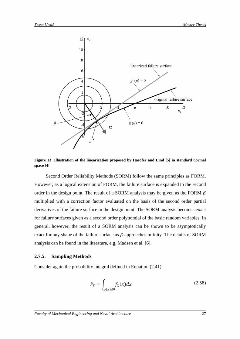
Tessa Uroić Master Thesis
Figure 13 Illustration of the linearization proposed by Hasofer and Lind [5] in standard normal space [4]
Second Order Reliability Methods (SORM) follow the same principles as FORM.
However, as a logical extension of FORM, the failure surface is expanded to the second
order in the design point. The result of a SORM analysis may be given as the FORM 𝛽
multiplied with a correction factor evaluated on the basis of the second order partial
derivatives of the failure surface in the design point. The SORM analysis becomes exact
for failure surfaces given as a second order polynomial of the basic random variables. In
general, however, the result of a SORM analysis can be shown to be asymptotically
exact for any shape of the failure surface as 𝛽 approaches infinity. The details of SORM
analysis can be found in the literature, e.g. Madsen et al. [6].
2.7.5. Sampling Methods
Consider again the probability integral defined in Equation (2.41):
𝑃𝐹 = � 𝑓𝑋(𝑥)𝑑𝑥𝑔(𝑥)≤0
(2.58)
_____________________________________________________________________________________ Faculty of Mechanical Engineering and Naval Architecture 27
Tessa Uroić Master Thesis
It has been seen that FORM methods may successfully be applied for the evaluation of
this integral. The integral may also be estimated by so-called sampling techniques. In
the literature, a large variety of simulation techniques can be found. Here it is just noted
that sampling techniques have proven their value especially for the problems where the
representation of the limit state function is associated with difficulties. Such cases are
e.g. when the limit state function is not differentiable or when several design points
contribute to the failure probability.
However, as all sampling techniques have their origin in the so-called crude
Monte Carlo Method, the principles of which will be briefly outlined below.
The basis for sampling techniques is well illustrated by rewriting the probability
integral in Eq. (2.58) by means of an indicator function:
𝑃𝐹 = � 𝑓𝑋(𝑥)𝑑𝑥𝑔(𝑥)≤0
= �𝐼[𝑔(𝑥) ≤ 0]𝑓𝑋(𝑥)𝑑𝑥 (2.59)
where the integration domain is changed from the part of the sample space of the vector
𝑋 = 𝑋1,𝑋2, … ,𝑋𝑛 for which 𝑔(𝑥) ≤ 0, to the entire sample space of 𝑋 and where
𝐼[𝑔(𝑥) ≤ 0] is an indicator function equal to 1 if 𝑔(𝑥) ≤ 0 and otherwise equal to zero.
Equation (2.59) is in this way seen to yield the expected value of the indicator function
𝐼[𝑔(𝑥) ≤ 0]. Therefore, if now 𝑁 realizations of the vector 𝑋, i.e. 𝑥𝑗 , 𝑗 = 1,2, … ,𝑁 are
sampled it follows from sample statistics that:
𝑃𝐹 =1𝑁�𝐼[𝑔(𝑥) ≤ 0]𝑁
𝑗=1
(2.60)
is an unbiased estimator of the failure probability 𝑃𝐹.
The principle of the crude Monte Carlo sampling technique rests directly on the
application of Equation (2.60). A large number of realizations of the basic random
variables 𝑋, i.e. 𝑥𝑗 , 𝑗 = 1,2, … ,𝑁 are generated and for each of the outcomes 𝑥𝑗 it is
checked whether or not the limit state function taken in 𝑥𝑗 is positive. All the samples
for which this is not the case are counted (𝑛𝐹) and after 𝑁 simulations the failure
probability 𝑃𝐹 may be estimated through:
_____________________________________________________________________________________ Faculty of Mechanical Engineering and Naval Architecture 28
Tessa Uroić Master Thesis
𝑃𝐹 =𝑛𝐹𝑁
(2.61)
which then may be considered a sample expected value of the probability of failure. In
fact, for 𝑁 → ∞ the estimate of the failure probability becomes exact. However,
simulations are often costly in computation time and the uncertainty of the estimate is
thus of interest. It is easily realized that the coefficient of variation of the estimate is
proportional to 1 √𝑛𝐹⁄ .
In this chapter, basics of probability theory were introduced: the three axioms of
probability theory, conditional probabilities, useful characteristics of the data (central
measures, dispersion measures, etc.), uncertainty modeling with random variables, as
well as first order reliability methods. In the next section, optimization capabilities of
Dakota software package will be presented.
_____________________________________________________________________________________ Faculty of Mechanical Engineering and Naval Architecture 29
Tessa Uroić Master Thesis
3. Dakota Software Package and Optimization Capabilities
In the previous chapter, basics of probability theory were introduced. In this
section, open source optimization software, Dakota, will be presented and its
optimization capabilities overviewed, [7].
Dakota (Design Analysis Kit for Optimization and Terascale Applications) is a
multilevel parallel object-oriented open source framework for design optimization,
parameter estimation, uncertainty quantification and sensitivity analysis [7]. Dakota
delivers a variety of iterative methods and strategies, and the ability to flexibly interface
them to simulation code. Recent versions go beyond optimization to include other
iterative analysis methods such as uncertainty quantification with nondeterministic
propagation methods, parameter estimation with nonlinear least squares solution
methods, and sensitivity/variance analysis with general-purpose design of experiments
and parameter study capabilities.
The principal classes of Dakota algorithms, with brief descriptions, are
summarized:
Parameter studies: Parameter studies employ deterministic designs to explore
the effect of parametric changes within simulation models, yielding one form
of sensitivity analysis. They can help assess simulation characteristics such as
smoothness, multi-modality, robustness, and nonlinearity, which affect the
choice of algorithms and controls in follow-on optimization and uncertainty
quantification studies.
Design of experiments: Design and analysis of computer experiments (DACE)
techniques are often used to explore the parameter space of an engineering
design problem, for example to perform global sensitivity analysis. DACE
methods can help reach conclusions similar to parameter studies, but the
primary goal of these methods is to generate good coverage of the input
parameter space.
Uncertainty quantification: Uncertainty quantification methods (also referred
to as nondeterministic analysis methods) compute probabilistic information
about response functions based on simulations performed according to
_____________________________________________________________________________________ Faculty of Mechanical Engineering and Naval Architecture 30
Tessa Uroić Master Thesis
specified input parameter probability distributions. Put another way, these
methods perform a forward uncertainty propagation in which probability
information for input parameters is mapped to probability information for
output response functions.
Optimization: Optimization solvers seek to minimize cost or maximize system
performance, as predicted by the simulation model, subject to constraints on
input variables or secondary simulation responses. Categories of algorithms
include gradient-based, derivative-free and global optimization. Dakota also
includes capabilities for multi-objective trade-off optimization and automatic
scaling of problem formulations. Advanced Dakota approaches include hybrid
(multi-method), multi-start local and Pareto-set optimization.
Calibration: Calibration algorithms seek to maximize agreement between
simulation outputs and experimental-data (or desired outputs). They are used to
solve inverse problems (often referred to as parameter estimation or least-
squares problems).
There are also more sophisticated strategies such as hybrid optimization, surrogate-
based optimization, optimization under uncertainty and mixed aleatory/epistemic
uncertainty quantification.
3.1. Optimization
Optimization is a discipline of numerical mathematics which aims to improve the
operation of a system or process as good as possible in some defined sense. [3]
Optimization algorithms work to minimize (or maximize) an objective function,
typically calculated by the user simulation code, subject to constraints on design
variables and responses.
_____________________________________________________________________________________ Faculty of Mechanical Engineering and Naval Architecture 31
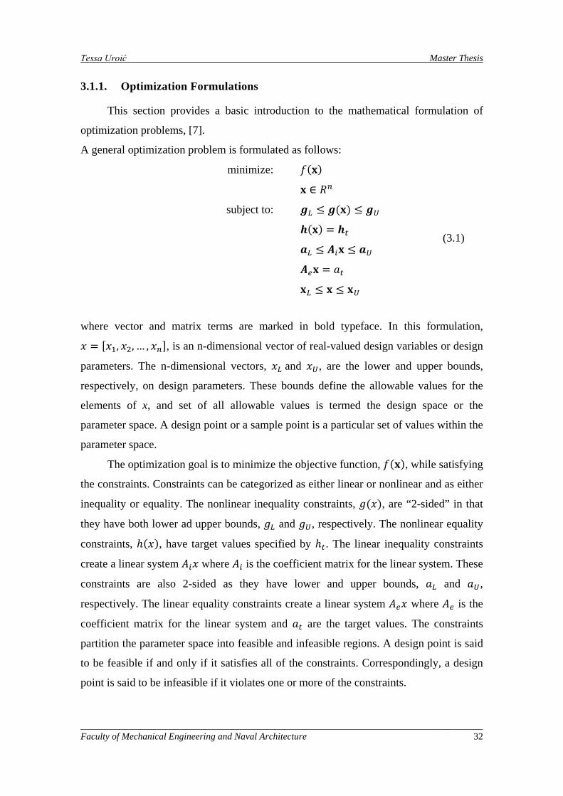
Tessa Uroić Master Thesis
3.1.1. Optimization Formulations
This section provides a basic introduction to the mathematical formulation of
optimization problems, [7].
A general optimization problem is formulated as follows:
minimize: 𝑓(𝐱)
𝐱 ∈ 𝑅𝑛
subject to: 𝒈𝐿 ≤ 𝒈(𝐱) ≤ 𝒈𝑈
𝒉(𝐱) = 𝒉𝑡
𝒂𝐿 ≤ 𝑨𝑖𝐱 ≤ 𝒂𝑈
𝑨𝑒𝐱 = 𝑎𝑡
𝐱𝐿 ≤ 𝐱 ≤ 𝐱𝑈
(3.1)
where vector and matrix terms are marked in bold typeface. In this formulation,
𝑥 = [𝑥1, 𝑥2, … , 𝑥𝑛], is an n-dimensional vector of real-valued design variables or design
parameters. The n-dimensional vectors, 𝑥𝐿 and 𝑥𝑈, are the lower and upper bounds,
respectively, on design parameters. These bounds define the allowable values for the
elements of x, and set of all allowable values is termed the design space or the
parameter space. A design point or a sample point is a particular set of values within the
parameter space.
The optimization goal is to minimize the objective function, 𝑓(𝐱), while satisfying
the constraints. Constraints can be categorized as either linear or nonlinear and as either
inequality or equality. The nonlinear inequality constraints, 𝑔(𝑥), are “2-sided” in that
they have both lower ad upper bounds, 𝑔𝐿 and 𝑔𝑈, respectively. The nonlinear equality
constraints, ℎ(𝑥), have target values specified by ℎ𝑡. The linear inequality constraints
create a linear system 𝐴𝑖𝑥 where 𝐴𝑖 is the coefficient matrix for the linear system. These
constraints are also 2-sided as they have lower and upper bounds, 𝑎𝐿 and 𝑎𝑈,
respectively. The linear equality constraints create a linear system 𝐴𝑒𝑥 where 𝐴𝑒 is the
coefficient matrix for the linear system and 𝑎𝑡 are the target values. The constraints
partition the parameter space into feasible and infeasible regions. A design point is said
to be feasible if and only if it satisfies all of the constraints. Correspondingly, a design
point is said to be infeasible if it violates one or more of the constraints.
_____________________________________________________________________________________ Faculty of Mechanical Engineering and Naval Architecture 32
Tessa Uroić Master Thesis
Many different methods exist to solve the optimization problem given by
Equation (3.1), all of which iterate on x in some manner. That is, an initial value for
each parameter in x is chosen, the response quantities, 𝑓(𝑥), 𝑔(𝑥), ℎ(𝑥), are computed,
often by running a simulation, and some algorithm is applied to generate a new x that
will either reduce the objective function, reduce the amount of infeasibility, or both. To
facilitate a general presentation of these methods, three criteria will be used in the
following discussion to differentiate them: optimization problem type, search goal, and
search method.
The optimization problem type can be characterized both by types of constraints
present in the problem and by the linearity or nonlinearity of the objective and
constraint functions. For constraint categorization, a hierarchy of complexity exists for
optimization algorithms, ranging from simple bound constraints, through linear
constraints, to full nonlinear constraints. By the nature of this increasing complexity,
optimization problem categorizations are inclusive of all constraint types up to a
particular level of complexity. That is, an unconstrained problem has no constraints, a
bound-constrained problem has only lower and upper bounds on the design parameters,
a linearly-constrained problem has both linear and bound constraints, and a nonlinearly-
constrained problem may contain the full range of nonlinear, linear, and bound
constraints. If all of the linear and nonlinear constraints are equality constraints, then
this is referred to as an equality-constrained problem, and if all of the linear and
nonlinear constraints are inequality constraints, then this is referred to as an inequality-
constrained problem. Further categorizations can be made based on the linearity of the
objective and constraint functions. A problem where the objective function and all
constraints are linear is called a linear programming (LP) problem. These types of
problems commonly arise in scheduling, logistics, and resource allocation applications.
Likewise, a problem where at least some of the objective and constraint functions are
nonlinear is called a nonlinear programming (NLP) problem. These NLP problems
predominate in engineering applications.
The search goal refers to the ultimate objective of the optimization algorithm, i.e.,
either global or local optimization. In global optimization, the goal is to find the design
point that gives the lowest feasible objective function value over the entire parameter
space. In contrast, in local optimization, the goal is to find a design point that is lowest
_____________________________________________________________________________________ Faculty of Mechanical Engineering and Naval Architecture 33
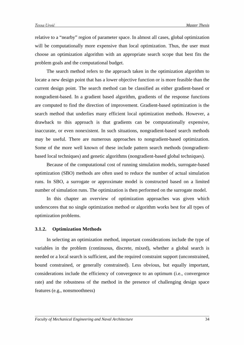
Tessa Uroić Master Thesis
relative to a “nearby” region of parameter space. In almost all cases, global optimization
will be computationally more expensive than local optimization. Thus, the user must
choose an optimization algorithm with an appropriate search scope that best fits the
problem goals and the computational budget.
The search method refers to the approach taken in the optimization algorithm to
locate a new design point that has a lower objective function or is more feasible than the
current design point. The search method can be classified as either gradient-based or
nongradient-based. In a gradient based algorithm, gradients of the response functions
are computed to find the direction of improvement. Gradient-based optimization is the
search method that underlies many efficient local optimization methods. However, a
drawback to this approach is that gradients can be computationally expensive,
inaccurate, or even nonexistent. In such situations, nongradient-based search methods
may be useful. There are numerous approaches to nongradient-based optimization.
Some of the more well known of these include pattern search methods (nongradient-
based local techniques) and genetic algorithms (nongradient-based global techniques).
Because of the computational cost of running simulation models, surrogate-based
optimization (SBO) methods are often used to reduce the number of actual simulation
runs. In SBO, a surrogate or approximate model is constructed based on a limited
number of simulation runs. The optimization is then performed on the surrogate model.
In this chapter an overview of optimization approaches was given which
underscores that no single optimization method or algorithm works best for all types of
optimization problems.
3.1.2. Optimization Methods
In selecting an optimization method, important considerations include the type of
variables in the problem (continuous, discrete, mixed), whether a global search is
needed or a local search is sufficient, and the required constraint support (unconstrained,
bound constrained, or generally constrained). Less obvious, but equally important,
considerations include the efficiency of convergence to an optimum (i.e., convergence
rate) and the robustness of the method in the presence of challenging design space
features (e.g., nonsmoothness)
_____________________________________________________________________________________ Faculty of Mechanical Engineering and Naval Architecture 34
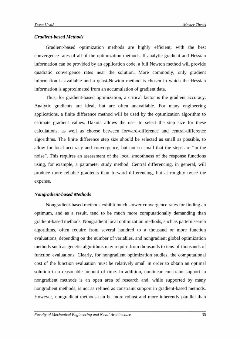
Tessa Uroić Master Thesis
Gradient-based Methods
Gradient-based optimization methods are highly efficient, with the best
convergence rates of all of the optimization methods. If analytic gradient and Hessian
information can be provided by an application code, a full Newton method will provide
quadratic convergence rates near the solution. More commonly, only gradient
information is available and a quasi-Newton method is chosen in which the Hessian
information is approximated from an accumulation of gradient data.
Thus, for gradient-based optimization, a critical factor is the gradient accuracy.
Analytic gradients are ideal, but are often unavailable. For many engineering
applications, a finite difference method will be used by the optimization algorithm to
estimate gradient values. Dakota allows the user to select the step size for these
calculations, as well as choose between forward-difference and central-difference
algorithms. The finite difference step size should be selected as small as possible, to
allow for local accuracy and convergence, but not so small that the steps are “in the
noise”. This requires an assessment of the local smoothness of the response functions
using, for example, a parameter study method. Central differencing, in general, will
produce more reliable gradients than forward differencing, but at roughly twice the
expense.
Nongradient-based Methods
Nongradient-based methods exhibit much slower convergence rates for finding an
optimum, and as a result, tend to be much more computationally demanding than
gradient-based methods. Nongradient local optimization methods, such as pattern search
algorithms, often require from several hundred to a thousand or more function
evaluations, depending on the number of variables, and nongradient global optimization
methods such as genetic algorithms may require from thousands to tens-of-thousands of
function evaluations. Clearly, for nongradient optimization studies, the computational
cost of the function evaluation must be relatively small in order to obtain an optimal
solution in a reasonable amount of time. In addition, nonlinear constraint support in
nongradient methods is an open area of research and, while supported by many
nongradient methods, is not as refined as constraint support in gradient-based methods.
However, nongradient methods can be more robust and more inherently parallel than
_____________________________________________________________________________________ Faculty of Mechanical Engineering and Naval Architecture 35
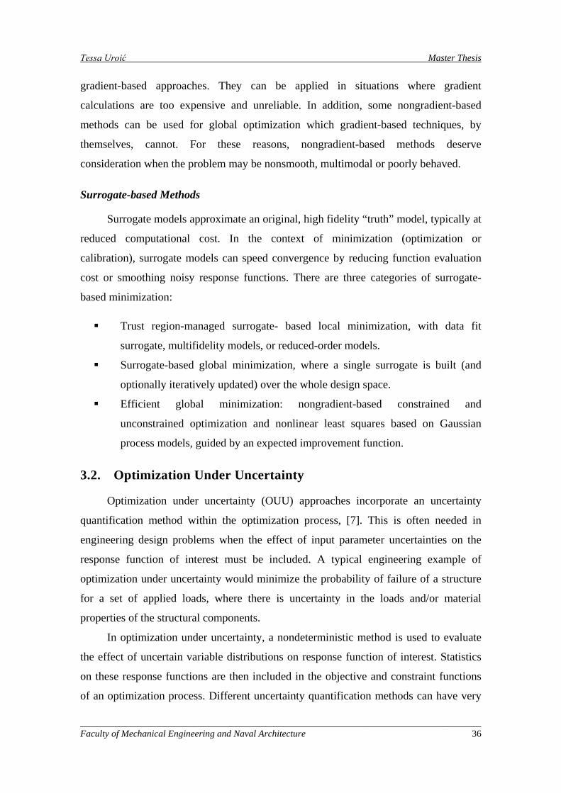
Tessa Uroić Master Thesis
gradient-based approaches. They can be applied in situations where gradient
calculations are too expensive and unreliable. In addition, some nongradient-based
methods can be used for global optimization which gradient-based techniques, by
themselves, cannot. For these reasons, nongradient-based methods deserve
consideration when the problem may be nonsmooth, multimodal or poorly behaved.
Surrogate-based Methods
Surrogate models approximate an original, high fidelity “truth” model, typically at
reduced computational cost. In the context of minimization (optimization or
calibration), surrogate models can speed convergence by reducing function evaluation
cost or smoothing noisy response functions. There are three categories of surrogate-
based minimization:
Trust region-managed surrogate- based local minimization, with data fit
surrogate, multifidelity models, or reduced-order models.
Surrogate-based global minimization, where a single surrogate is built (and
optionally iteratively updated) over the whole design space.
Efficient global minimization: nongradient-based constrained and
unconstrained optimization and nonlinear least squares based on Gaussian
process models, guided by an expected improvement function.
3.2. Optimization Under Uncertainty
Optimization under uncertainty (OUU) approaches incorporate an uncertainty
quantification method within the optimization process, [7]. This is often needed in
engineering design problems when the effect of input parameter uncertainties on the
response function of interest must be included. A typical engineering example of
optimization under uncertainty would minimize the probability of failure of a structure
for a set of applied loads, where there is uncertainty in the loads and/or material
properties of the structural components.
In optimization under uncertainty, a nondeterministic method is used to evaluate
the effect of uncertain variable distributions on response function of interest. Statistics
on these response functions are then included in the objective and constraint functions
of an optimization process. Different uncertainty quantification methods can have very
_____________________________________________________________________________________ Faculty of Mechanical Engineering and Naval Architecture 36
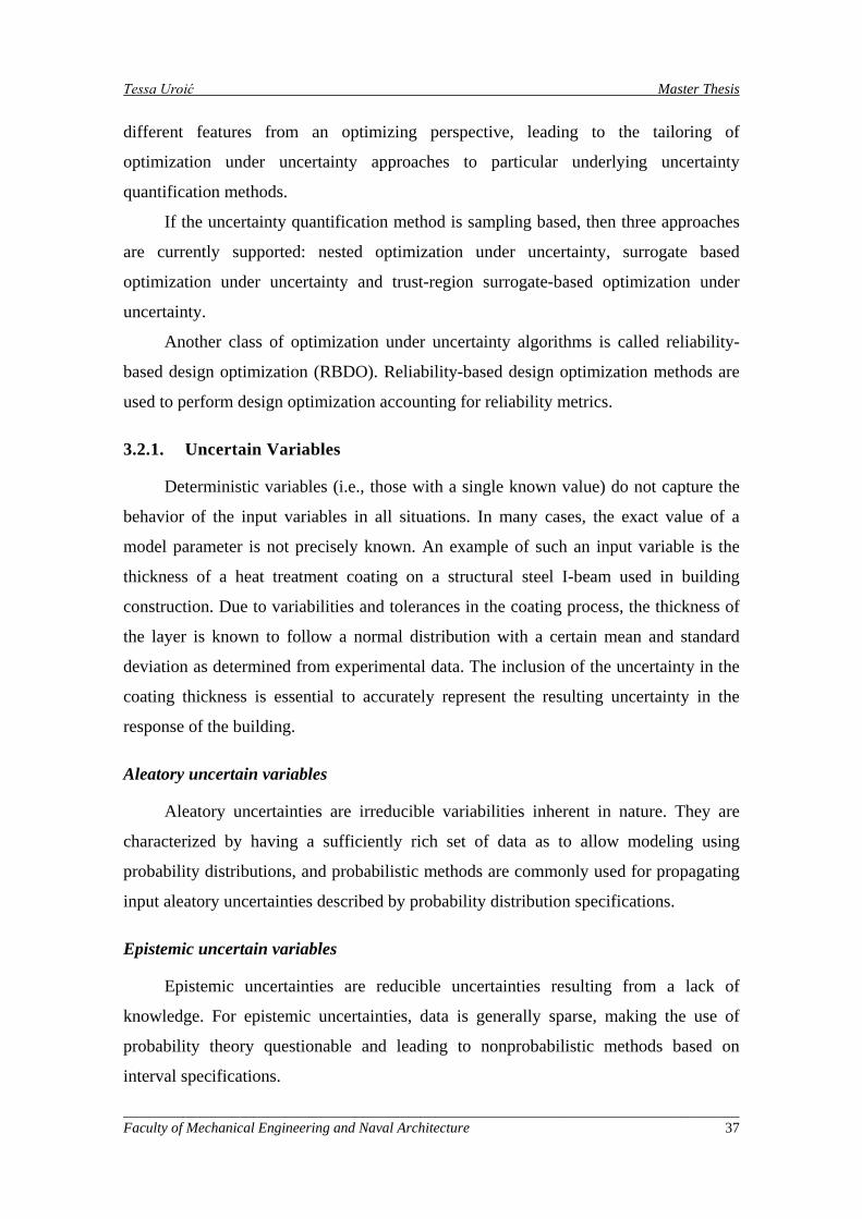
Tessa Uroić Master Thesis
different features from an optimizing perspective, leading to the tailoring of
optimization under uncertainty approaches to particular underlying uncertainty
quantification methods.
If the uncertainty quantification method is sampling based, then three approaches
are currently supported: nested optimization under uncertainty, surrogate based
optimization under uncertainty and trust-region surrogate-based optimization under
uncertainty.
Another class of optimization under uncertainty algorithms is called reliability-
based design optimization (RBDO). Reliability-based design optimization methods are
used to perform design optimization accounting for reliability metrics.
3.2.1. Uncertain Variables
Deterministic variables (i.e., those with a single known value) do not capture the
behavior of the input variables in all situations. In many cases, the exact value of a
model parameter is not precisely known. An example of such an input variable is the
thickness of a heat treatment coating on a structural steel I-beam used in building
construction. Due to variabilities and tolerances in the coating process, the thickness of
the layer is known to follow a normal distribution with a certain mean and standard
deviation as determined from experimental data. The inclusion of the uncertainty in the
coating thickness is essential to accurately represent the resulting uncertainty in the
response of the building.
Aleatory uncertain variables
Aleatory uncertainties are irreducible variabilities inherent in nature. They are
characterized by having a sufficiently rich set of data as to allow modeling using
probability distributions, and probabilistic methods are commonly used for propagating
input aleatory uncertainties described by probability distribution specifications.
Epistemic uncertain variables
Epistemic uncertainties are reducible uncertainties resulting from a lack of
knowledge. For epistemic uncertainties, data is generally sparse, making the use of
probability theory questionable and leading to nonprobabilistic methods based on
interval specifications.
_____________________________________________________________________________________ Faculty of Mechanical Engineering and Naval Architecture 37
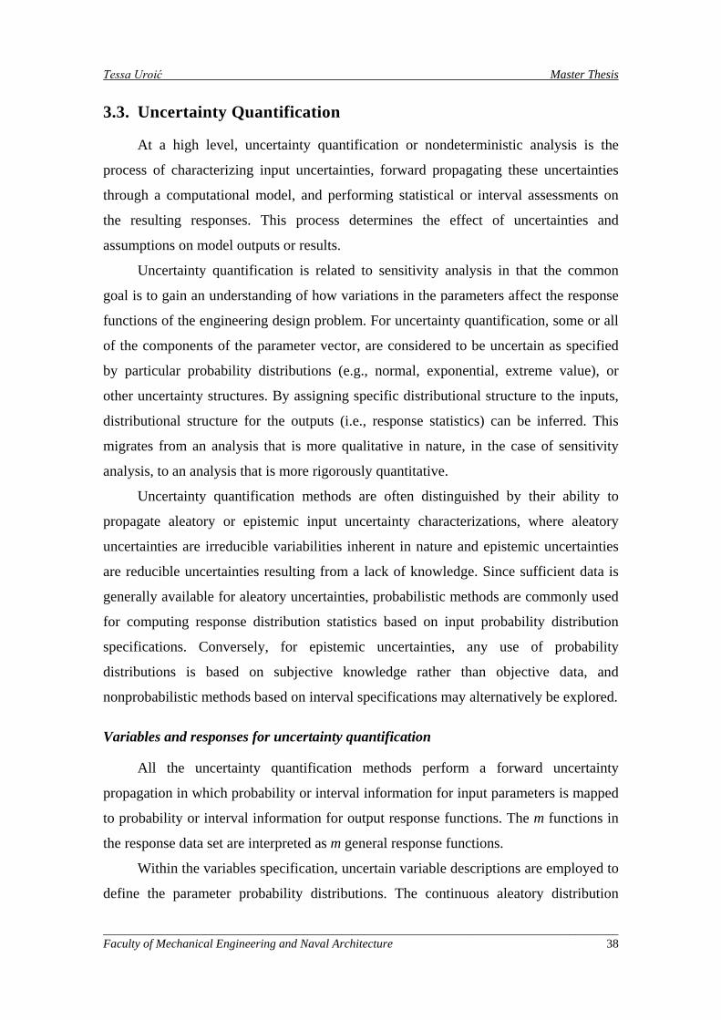
Tessa Uroić Master Thesis
3.3. Uncertainty Quantification
At a high level, uncertainty quantification or nondeterministic analysis is the
process of characterizing input uncertainties, forward propagating these uncertainties
through a computational model, and performing statistical or interval assessments on
the resulting responses. This process determines the effect of uncertainties and
assumptions on model outputs or results.
Uncertainty quantification is related to sensitivity analysis in that the common
goal is to gain an understanding of how variations in the parameters affect the response
functions of the engineering design problem. For uncertainty quantification, some or all
of the components of the parameter vector, are considered to be uncertain as specified
by particular probability distributions (e.g., normal, exponential, extreme value), or
other uncertainty structures. By assigning specific distributional structure to the inputs,
distributional structure for the outputs (i.e., response statistics) can be inferred. This
migrates from an analysis that is more qualitative in nature, in the case of sensitivity
analysis, to an analysis that is more rigorously quantitative.
Uncertainty quantification methods are often distinguished by their ability to
propagate aleatory or epistemic input uncertainty characterizations, where aleatory
uncertainties are irreducible variabilities inherent in nature and epistemic uncertainties
are reducible uncertainties resulting from a lack of knowledge. Since sufficient data is
generally available for aleatory uncertainties, probabilistic methods are commonly used
for computing response distribution statistics based on input probability distribution
specifications. Conversely, for epistemic uncertainties, any use of probability
distributions is based on subjective knowledge rather than objective data, and
nonprobabilistic methods based on interval specifications may alternatively be explored.
Variables and responses for uncertainty quantification
All the uncertainty quantification methods perform a forward uncertainty
propagation in which probability or interval information for input parameters is mapped
to probability or interval information for output response functions. The m functions in
the response data set are interpreted as m general response functions.
Within the variables specification, uncertain variable descriptions are employed to
define the parameter probability distributions. The continuous aleatory distribution
_____________________________________________________________________________________ Faculty of Mechanical Engineering and Naval Architecture 38
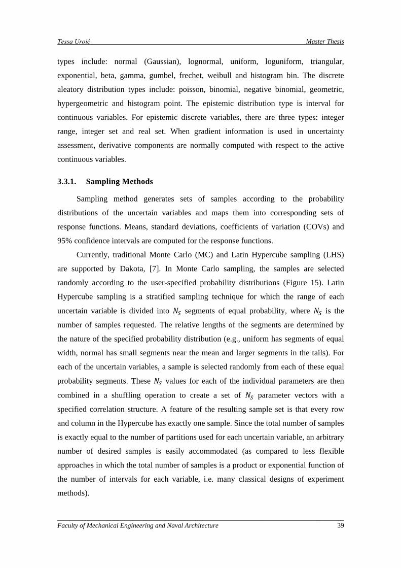
Tessa Uroić Master Thesis
types include: normal (Gaussian), lognormal, uniform, loguniform, triangular,
exponential, beta, gamma, gumbel, frechet, weibull and histogram bin. The discrete
aleatory distribution types include: poisson, binomial, negative binomial, geometric,
hypergeometric and histogram point. The epistemic distribution type is interval for
continuous variables. For epistemic discrete variables, there are three types: integer
range, integer set and real set. When gradient information is used in uncertainty
assessment, derivative components are normally computed with respect to the active
continuous variables.
3.3.1. Sampling Methods
Sampling method generates sets of samples according to the probability
distributions of the uncertain variables and maps them into corresponding sets of
response functions. Means, standard deviations, coefficients of variation (COVs) and
95% confidence intervals are computed for the response functions.
Currently, traditional Monte Carlo (MC) and Latin Hypercube sampling (LHS)
are supported by Dakota, [7]. In Monte Carlo sampling, the samples are selected
randomly according to the user-specified probability distributions (Figure 15). Latin
Hypercube sampling is a stratified sampling technique for which the range of each
uncertain variable is divided into 𝑁𝑆 segments of equal probability, where 𝑁𝑆 is the
number of samples requested. The relative lengths of the segments are determined by
the nature of the specified probability distribution (e.g., uniform has segments of equal
width, normal has small segments near the mean and larger segments in the tails). For
each of the uncertain variables, a sample is selected randomly from each of these equal
probability segments. These 𝑁𝑆 values for each of the individual parameters are then
combined in a shuffling operation to create a set of 𝑁𝑆 parameter vectors with a
specified correlation structure. A feature of the resulting sample set is that every row
and column in the Hypercube has exactly one sample. Since the total number of samples
is exactly equal to the number of partitions used for each uncertain variable, an arbitrary
number of desired samples is easily accommodated (as compared to less flexible
approaches in which the total number of samples is a product or exponential function of
the number of intervals for each variable, i.e. many classical designs of experiment
methods).
_____________________________________________________________________________________ Faculty of Mechanical Engineering and Naval Architecture 39
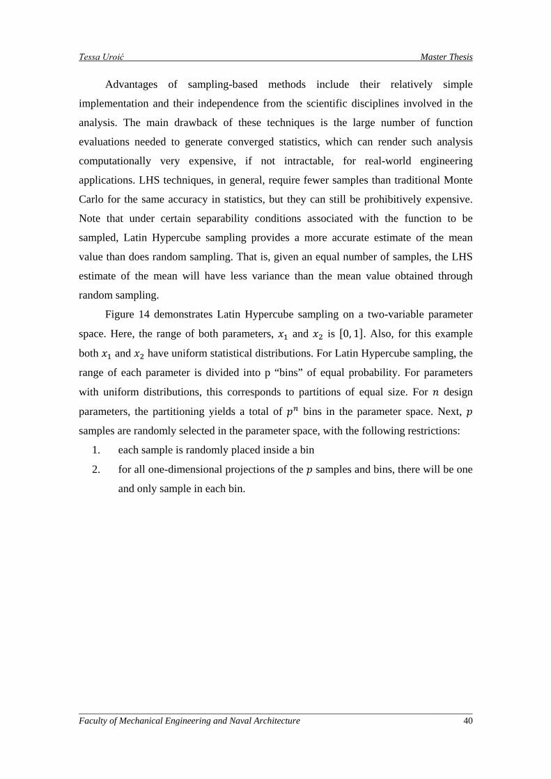
Tessa Uroić Master Thesis
Advantages of sampling-based methods include their relatively simple
implementation and their independence from the scientific disciplines involved in the
analysis. The main drawback of these techniques is the large number of function
evaluations needed to generate converged statistics, which can render such analysis
computationally very expensive, if not intractable, for real-world engineering
applications. LHS techniques, in general, require fewer samples than traditional Monte
Carlo for the same accuracy in statistics, but they can still be prohibitively expensive.
Note that under certain separability conditions associated with the function to be
sampled, Latin Hypercube sampling provides a more accurate estimate of the mean
value than does random sampling. That is, given an equal number of samples, the LHS
estimate of the mean will have less variance than the mean value obtained through
random sampling.
Figure 14 demonstrates Latin Hypercube sampling on a two-variable parameter
space. Here, the range of both parameters, 𝑥1 and 𝑥2 is [0, 1]. Also, for this example
both 𝑥1 and 𝑥2 have uniform statistical distributions. For Latin Hypercube sampling, the
range of each parameter is divided into p “bins” of equal probability. For parameters
with uniform distributions, this corresponds to partitions of equal size. For 𝑛 design
parameters, the partitioning yields a total of 𝑝𝑛 bins in the parameter space. Next, 𝑝
samples are randomly selected in the parameter space, with the following restrictions:
1. each sample is randomly placed inside a bin
2. for all one-dimensional projections of the 𝑝 samples and bins, there will be one
and only sample in each bin.
_____________________________________________________________________________________ Faculty of Mechanical Engineering and Naval Architecture 40
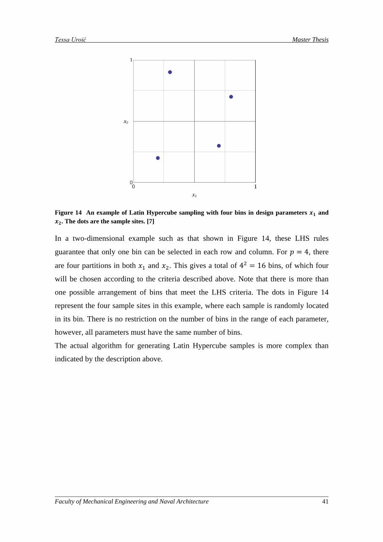
Tessa Uroić Master Thesis
Figure 14 An example of Latin Hypercube sampling with four bins in design parameters 𝒙𝟏 and 𝒙𝟐. The dots are the sample sites. [7]
In a two-dimensional example such as that shown in Figure 14, these LHS rules
guarantee that only one bin can be selected in each row and column. For 𝑝 = 4, there
are four partitions in both 𝑥1 and 𝑥2. This gives a total of 42 = 16 bins, of which four
will be chosen according to the criteria described above. Note that there is more than
one possible arrangement of bins that meet the LHS criteria. The dots in Figure 14
represent the four sample sites in this example, where each sample is randomly located
in its bin. There is no restriction on the number of bins in the range of each parameter,
however, all parameters must have the same number of bins.
The actual algorithm for generating Latin Hypercube samples is more complex than
indicated by the description above.
_____________________________________________________________________________________ Faculty of Mechanical Engineering and Naval Architecture 41
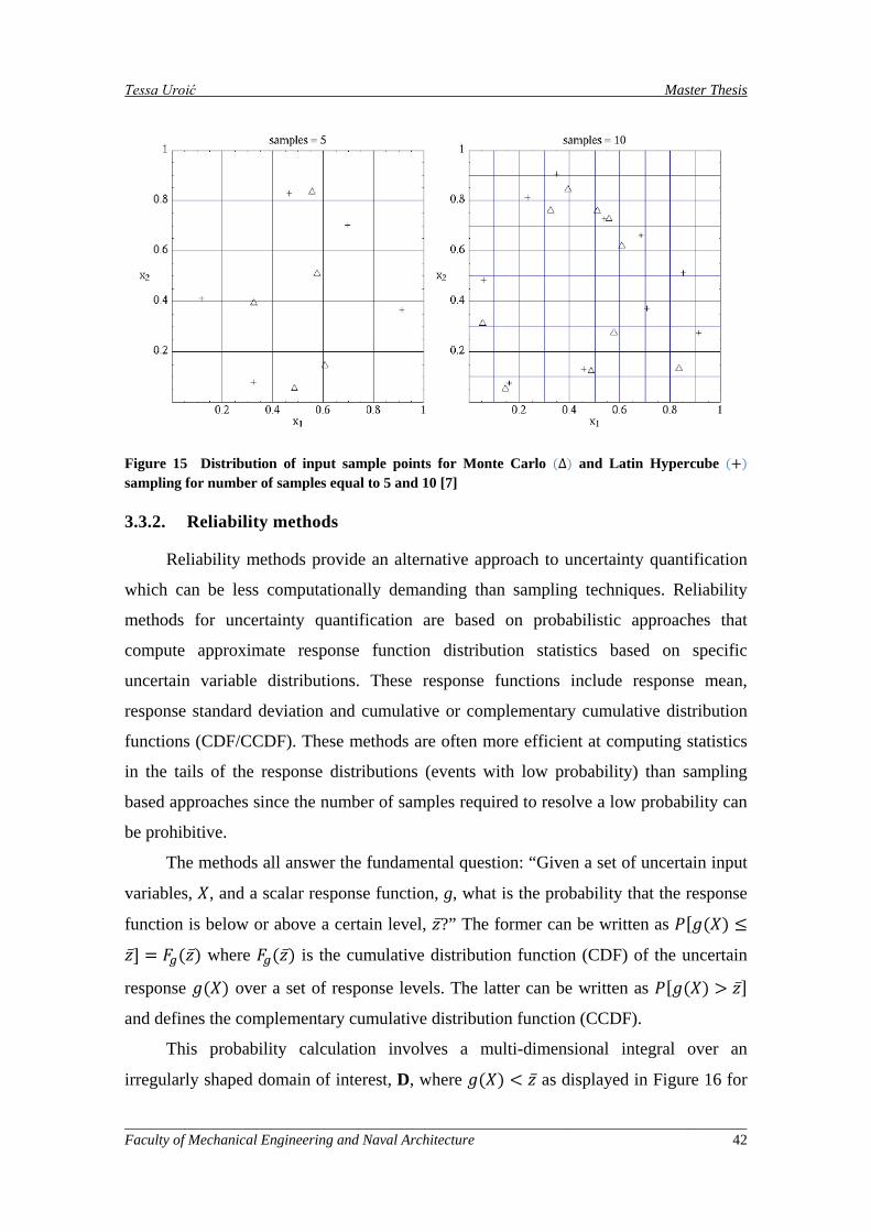
Tessa Uroić Master Thesis
Figure 15 Distribution of input sample points for Monte Carlo (∆) and Latin Hypercube (+) sampling for number of samples equal to 5 and 10 [7]
3.3.2. Reliability methods
Reliability methods provide an alternative approach to uncertainty quantification
which can be less computationally demanding than sampling techniques. Reliability
methods for uncertainty quantification are based on probabilistic approaches that
compute approximate response function distribution statistics based on specific
uncertain variable distributions. These response functions include response mean,
response standard deviation and cumulative or complementary cumulative distribution
functions (CDF/CCDF). These methods are often more efficient at computing statistics
in the tails of the response distributions (events with low probability) than sampling
based approaches since the number of samples required to resolve a low probability can
be prohibitive.
The methods all answer the fundamental question: “Given a set of uncertain input
variables, 𝑋, and a scalar response function, g, what is the probability that the response
function is below or above a certain level, 𝑧̅?” The former can be written as 𝑃[𝑔(𝑋) ≤
𝑧̅] = 𝐹𝑔(𝑧̅) where 𝐹𝑔(𝑧̅) is the cumulative distribution function (CDF) of the uncertain
response 𝑔(𝑋) over a set of response levels. The latter can be written as 𝑃[𝑔(𝑋) > 𝑧̅]
and defines the complementary cumulative distribution function (CCDF).
This probability calculation involves a multi-dimensional integral over an
irregularly shaped domain of interest, D, where 𝑔(𝑋) < 𝑧̅ as displayed in Figure 16 for
_____________________________________________________________________________________ Faculty of Mechanical Engineering and Naval Architecture 42
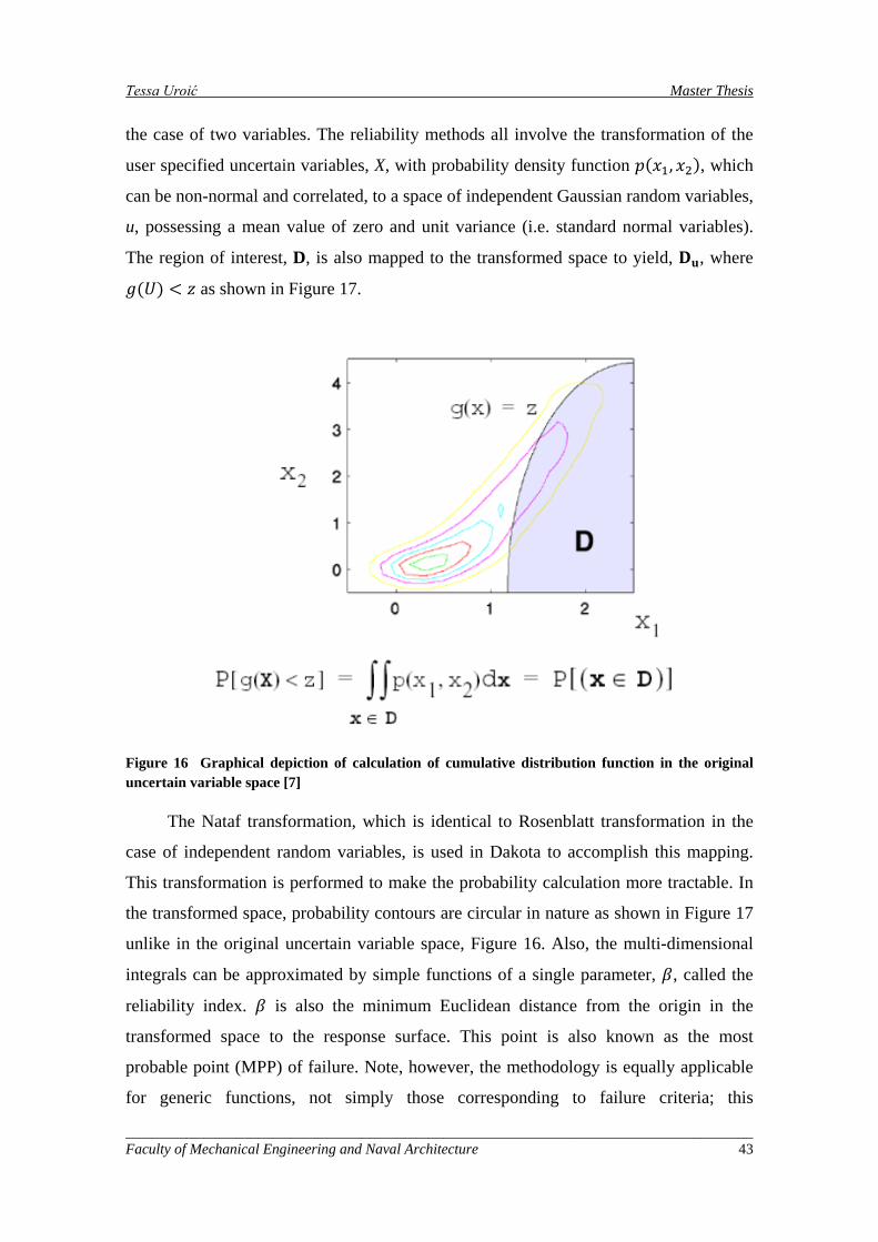
Tessa Uroić Master Thesis
the case of two variables. The reliability methods all involve the transformation of the
user specified uncertain variables, X, with probability density function 𝑝(𝑥1, 𝑥2), which
can be non-normal and correlated, to a space of independent Gaussian random variables,
u, possessing a mean value of zero and unit variance (i.e. standard normal variables).
The region of interest, D, is also mapped to the transformed space to yield, 𝐃𝐮, where
𝑔(𝑈) < 𝑧 as shown in Figure 17.
Figure 16 Graphical depiction of calculation of cumulative distribution function in the original uncertain variable space [7]
The Nataf transformation, which is identical to Rosenblatt transformation in the
case of independent random variables, is used in Dakota to accomplish this mapping.
This transformation is performed to make the probability calculation more tractable. In
the transformed space, probability contours are circular in nature as shown in Figure 17
unlike in the original uncertain variable space, Figure 16. Also, the multi-dimensional
integrals can be approximated by simple functions of a single parameter, 𝛽, called the
reliability index. 𝛽 is also the minimum Euclidean distance from the origin in the
transformed space to the response surface. This point is also known as the most
probable point (MPP) of failure. Note, however, the methodology is equally applicable
for generic functions, not simply those corresponding to failure criteria; this
_____________________________________________________________________________________ Faculty of Mechanical Engineering and Naval Architecture 43
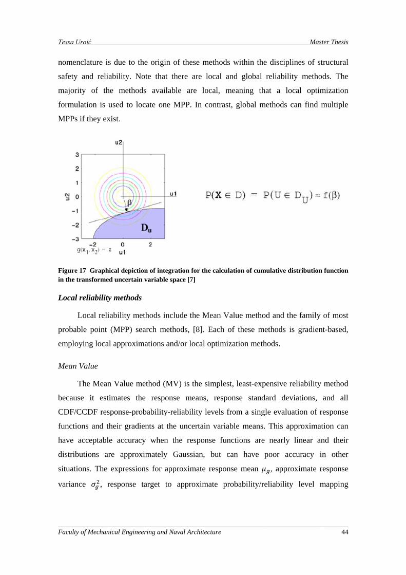
Tessa Uroić Master Thesis
nomenclature is due to the origin of these methods within the disciplines of structural
safety and reliability. Note that there are local and global reliability methods. The
majority of the methods available are local, meaning that a local optimization
formulation is used to locate one MPP. In contrast, global methods can find multiple
MPPs if they exist.
Figure 17 Graphical depiction of integration for the calculation of cumulative distribution function in the transformed uncertain variable space [7]
Local reliability methods
Local reliability methods include the Mean Value method and the family of most
probable point (MPP) search methods, [8]. Each of these methods is gradient-based,
employing local approximations and/or local optimization methods.
Mean Value
The Mean Value method (MV) is the simplest, least-expensive reliability method
because it estimates the response means, response standard deviations, and all
CDF/CCDF response-probability-reliability levels from a single evaluation of response
functions and their gradients at the uncertain variable means. This approximation can
have acceptable accuracy when the response functions are nearly linear and their
distributions are approximately Gaussian, but can have poor accuracy in other
situations. The expressions for approximate response mean 𝜇𝑔, approximate response
variance 𝜎𝑔2, response target to approximate probability/reliability level mapping
_____________________________________________________________________________________ Faculty of Mechanical Engineering and Naval Architecture 44
Tessa Uroić Master Thesis
(𝑧̅ → 𝑝,𝛽), and probability/reliability target to approximate response level mapping
��̅�, �̅� → 𝑧� are
𝜇𝑔 = 𝑔(𝜇𝑥) (3.2)
𝜎𝑔2 = ��𝐶𝑜𝑣(𝑖, 𝑗)𝑑𝑔𝑑𝑥𝑖𝑗𝑖
(𝜇𝑥)𝑑𝑔𝑑𝑥𝑗
(𝜇𝑥) (3.3)
𝑧̅ → 𝛽: 𝛽𝐶𝐷𝐹 =𝜇𝑔 − 𝑧̅𝜎𝑔
, 𝛽𝐶𝐶𝐷𝐹 =𝑧̅ − 𝜇𝑔𝜎𝑔
(3.4)
�̅� → 𝑧: 𝑧 = 𝜇𝑔 − 𝜎𝑔 ∙ 𝛽𝐶𝐷𝐹 , 𝑧 = 𝜇𝑔 + 𝜎𝑔 ∙ 𝛽𝐶𝐶𝐷𝐹 (3.5)
respectively, where x are the uncertain values in the space of the original uncertain
values (“x-space”), 𝑔(𝑥) is the limit state function (the response function for which
probability-response level pairs are needed), and 𝛽𝐶𝐷𝐹 and 𝛽𝐶𝐶𝐷𝐹 are the CDF and
CCDF reliability indices, respectively.
With the introduction of second-order limit state information, MV calculates a
second-order mean as
𝜇𝑔 = 𝑔(𝜇𝑥) +12��𝐶𝑜𝑣(𝑖, 𝑗)
𝑑2𝑔𝑑𝑥𝑖𝑑𝑥𝑗𝑗𝑖
(𝜇𝑥) (3.6)
This is commonly combined with a first order variance (Equation (3.3)), since second-
order variance involves higher order distribution moments (skewness, kurtosis) which
are often unavailable.
The first-order CDF probability 𝑝(𝑔 ≤ 𝑧), first order CCDF probability 𝑝(𝑔 >
𝑧), 𝛽𝐶𝐷𝐹 and 𝛽𝐶𝐶𝐷𝐹 are related to one another through:
𝑝(𝑔 ≤ 𝑧) = 𝛷(−𝛽𝐶𝐷𝐹) (3.7)
𝑝(𝑔 > 𝑧) = 𝛷(−𝛽𝐶𝐶𝐷𝐹) (3.8)
𝛽𝐶𝐷𝐹 = −𝛷−1(𝑝(𝑔 ≤ 𝑧)) (3.9)
_____________________________________________________________________________________ Faculty of Mechanical Engineering and Naval Architecture 45
Tessa Uroić Master Thesis
𝛽𝐶𝐶𝐷𝐹 = −𝛷−1(𝑝(𝑔 > 𝑧)) (3.10)
𝛽𝐶𝐷𝐹 = −𝛽𝐶𝐶𝐷𝐹 (3.11)
𝑝(𝑔 ≤ 𝑧) = 1 − 𝑝(𝑔 > 𝑧) (3.12)
where 𝛷( ) is the standard normal cumulative distribution function. A common
convention in the literature is to define g in such a way that the CDF probability for
response level z of zero (i.e., 𝑝(𝑔 ≤ 0)) is the response metric of interest. Dakota is not
restricted to this convention and is designed to support CDF or CCDF mappings for
general response, probability and reliability level sequences.
With the Mean Value method, it is possible to obtain importance factors
indicating the relative importance of input variables. The importance factors can be
viewed as an extension of linear sensitivity analysis combining deterministic gradient
information with input uncertainty information, i.e. input variable standard deviations.
The accuracy of the importance factors is contingent of the validity of the linear
approximation used to approximate the true response functions. The importance factors
are determined as:
𝐼𝑚𝑝𝐹𝑎𝑐𝑡𝑜𝑟𝑖 = �𝜎𝑥𝑖𝜎𝑔
𝑑𝑔𝑑𝑥𝑖
(𝜇𝑥)�2
(3.13)
In this chapter, optimization capabilities of Dakota optimization open source
software were overviewed. Methods for optimization under uncertainty were described.
In the following chapter, parameters and challenges of Multi-objective optimization will
be presented.
_____________________________________________________________________________________ Faculty of Mechanical Engineering and Naval Architecture 46
Tessa Uroić Master Thesis
4. Multi-objective Optimization
In the last chapter, optimization capabilities of Dakota optimization open source
software were overviewed. In this chapter, Multi-objective optimization will be
described, [9].
Multi-objective optimization implies that there are two or more objective
functions that we wish to optimize simultaneously. Often these are conflicting
objectives, such as cost and performance. The answer to a multi-objective problem is
usually not a single point. Rather, it is a set of points called the Pareto front. Each point
on the Pareto front satisfies the Pareto optimality criterion. which is stated as follows: a
feasible vector is Pareto optimal if there exists no other feasible vector which would
improve some objective without causing a simultaneous worsening in at least one other
objective. Thus, if a feasible point exists that can be improved on one or more
objectives simultaneously, it is not Pareto optimal: it is said to be “dominated” and the
points along the Pareto front are said to be “non-dominated”.
Mathematically speaking, a multi-objective problem consists of optimizing (i.e.
minimizing or maximizing) several objectives simultaneously, with a number of
inequality or equality constraints. The problem can be formally written as follows:
𝐹𝑖𝑛𝑑 𝑥 = (𝑥𝑖) ∀ 𝑖 = 1, 2, … ,𝑁𝑝𝑎𝑟𝑎𝑚
𝑠𝑢𝑐ℎ 𝑎𝑠 𝑓𝑖(𝑥) 𝑖𝑠 𝑎 𝑚𝑖𝑛𝑖𝑚𝑢𝑚 (𝑟𝑒𝑠𝑝.𝑚𝑎𝑥𝑖𝑚𝑢𝑚),∀ 𝑖 = 1,2, … ,𝑁𝑜𝑏𝑗
(4.1)
subject to:
𝑔𝑗(𝑥) = 0, ∀ 𝑗 = 1, 2, … ,𝑀 (4.2)
ℎ𝑘(𝑥) ≤ 0, ∀ 𝑘 = 1, 2, … ,𝐾 (4.3)
where 𝑥 is a vector containing the 𝑁𝑝𝑎𝑟𝑎𝑚 design parameters, (𝑓𝑖)𝑖=1…𝑁𝑜𝑏𝑗 the objective
functions and 𝑁𝑜𝑏𝑗 the number of objectives. In this study, only inequality constraints
are considered and are prescribed as bounded domains. In other words, upper and lower
limits are imposed on all parameters:
𝑥𝑖 ∈ �𝑥𝑖,𝑚𝑖𝑛; 𝑥𝑖,𝑚𝑎𝑥� 𝑖 = 1 …𝑁𝑝𝑎𝑟𝑎𝑚 (4.4)
_____________________________________________________________________________________ Faculty of Mechanical Engineering and Naval Architecture 47
Tessa Uroić Master Thesis
The objective function (𝑓𝑖)𝑖=1…𝑁𝑜𝑏𝑗 returns a vector containing the set of 𝑁𝑜𝑏𝑗
values associated with the elementary objectives to be optimized simultaneously. A
common practice to solve such a problem is to use a trade-off between the objectives by
linearly combining them using some fixed weights prescribed by the user. The resulting
single objective function is optimized. The firs limitation of this kind of approach is that
the choice of the weights associated with each objective obviously influences the
solution of the optimization problem. A bad choice can lead to completely sub-optimal
results in comparison with the solution obtained by considering the interrelated
objectives in an independent manner. Moreover, this method does not allow access to
all the set of optimal solutions.
The Evolutionary Algorithms are semi-stochastic methods, based on an analogy
with Darwin’s law of natural selection. Each configuration 𝑥 is considered as an
individual. The parameters 𝑥𝑖 represent its genes. The main principle is to consider a
population of 𝑁 individuals, i.e., a set of individuals covering the search domain and to
let it evolve along generations (or iterations) so that the best individuals survive and
have offsprings, i.e., are taken into account and allow to find better and better
configurations.
The characteristics of the EA are based on the approach proposed by Fonseca and
Fleming [10]. The genes (sometimes called characters) of the individuals (also called
strings or chromosomes) are the 𝑁𝑝𝑎𝑟𝑎𝑚 design parameters, encoded using a floating-
point representation. The initial population is a set of quasi-random configurations in
the domain defined by the limits imposed on the parameters. The creation of a new
generation from the previous one is performed by applying genetic operators to the
individuals of the present generation. The fitness-based selection is applied. At each
generation, the individuals are classified as a function of their corresponding objective
values, leading to a rank within the population and finally to a fitness. The probability
for an individual to participate in the reproduction process is determined by a
probability based on its fitness value, linearly calculated from its rank in the
classification. For example, for individual number 𝑖 in a group of 𝑁 individuals:
𝐹𝑖𝑡𝑛𝑒𝑠𝑠(𝑖) =𝑁 − 𝑟𝑎𝑛𝑘(𝑖) + 1
∑ (𝑁 − 𝑟𝑎𝑛𝑘(𝑗) − 1)𝑗 (4.5)
_____________________________________________________________________________________ Faculty of Mechanical Engineering and Naval Architecture 48
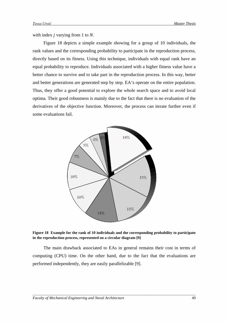
Tessa Uroić Master Thesis
with index 𝑗 varying from 1 to 𝑁.
Figure 18 depicts a simple example showing for a group of 10 individuals, the
rank values and the corresponding probability to participate in the reproduction process,
directly based on its fitness. Using this technique, individuals with equal rank have an
equal probability to reproduce. Individuals associated with a higher fitness value have a
better chance to survive and to take part in the reproduction process. In this way, better
and better generations are generated step by step. EA’s operate on the entire population.
Thus, they offer a good potential to explore the whole search space and to avoid local
optima. Their good robustness is mainly due to the fact that there is no evaluation of the
derivatives of the objective function. Moreover, the process can iterate further even if
some evaluations fail.
Figure 18 Example for the rank of 10 individuals and the corresponding probability to participate in the reproduction process, represented on a circular diagram [9]
The main drawback associated to EAs in general remains their cost in terms of
computing (CPU) time. On the other hand, due to the fact that the evaluations are
performed independently, they are easily parallelizable [9].
_____________________________________________________________________________________ Faculty of Mechanical Engineering and Naval Architecture 49
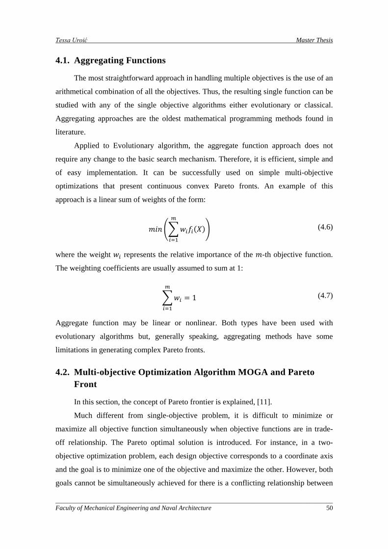
Tessa Uroić Master Thesis
4.1. Aggregating Functions
The most straightforward approach in handling multiple objectives is the use of an
arithmetical combination of all the objectives. Thus, the resulting single function can be
studied with any of the single objective algorithms either evolutionary or classical.
Aggregating approaches are the oldest mathematical programming methods found in
literature.
Applied to Evolutionary algorithm, the aggregate function approach does not
require any change to the basic search mechanism. Therefore, it is efficient, simple and
of easy implementation. It can be successfully used on simple multi-objective
optimizations that present continuous convex Pareto fronts. An example of this
approach is a linear sum of weights of the form:
𝑚𝑖𝑛 ��𝑤𝑖𝑓𝑖(𝑋)𝑚
𝑖=1
� (4.6)
where the weight 𝑤𝑖 represents the relative importance of the 𝑚-th objective function.
The weighting coefficients are usually assumed to sum at 1:
�𝑤𝑖 = 1𝑚
𝑖=1
(4.7)
Aggregate function may be linear or nonlinear. Both types have been used with
evolutionary algorithms but, generally speaking, aggregating methods have some
limitations in generating complex Pareto fronts.
4.2. Multi-objective Optimization Algorithm MOGA and Pareto Front
In this section, the concept of Pareto frontier is explained, [11].
Much different from single-objective problem, it is difficult to minimize or
maximize all objective function simultaneously when objective functions are in trade-
off relationship. The Pareto optimal solution is introduced. For instance, in a two-
objective optimization problem, each design objective corresponds to a coordinate axis
and the goal is to minimize one of the objective and maximize the other. However, both
goals cannot be simultaneously achieved for there is a conflicting relationship between
_____________________________________________________________________________________ Faculty of Mechanical Engineering and Naval Architecture 50
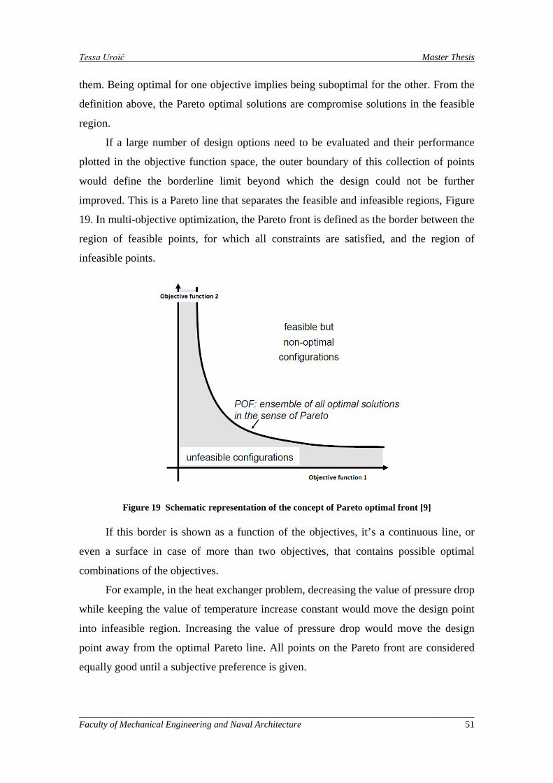
Tessa Uroić Master Thesis
them. Being optimal for one objective implies being suboptimal for the other. From the
definition above, the Pareto optimal solutions are compromise solutions in the feasible
region.
If a large number of design options need to be evaluated and their performance
plotted in the objective function space, the outer boundary of this collection of points
would define the borderline limit beyond which the design could not be further
improved. This is a Pareto line that separates the feasible and infeasible regions, Figure
19. In multi-objective optimization, the Pareto front is defined as the border between the
region of feasible points, for which all constraints are satisfied, and the region of
infeasible points.
Figure 19 Schematic representation of the concept of Pareto optimal front [9]
If this border is shown as a function of the objectives, it’s a continuous line, or
even a surface in case of more than two objectives, that contains possible optimal
combinations of the objectives.
For example, in the heat exchanger problem, decreasing the value of pressure drop
while keeping the value of temperature increase constant would move the design point
into infeasible region. Increasing the value of pressure drop would move the design
point away from the optimal Pareto line. All points on the Pareto front are considered
equally good until a subjective preference is given.
_____________________________________________________________________________________ Faculty of Mechanical Engineering and Naval Architecture 51

Tessa Uroić Master Thesis
Multi-objective genetic algorithm (MOGA) mimics the natural selection process
in which a superior creature evolves whilst inferior creatures fade out from their
population as generations go by [12]. There are many advantages of MOGA such as the
capability of exploring a large design space and no gradients are needed. But, the most
important one is that MOGA can compute multiple independent objective functions
simultaneously in one optimization run without converting multiple objective functions
into a single objective by weighted linear combination.
The optimization procedure of MOGA includes the following steps [13]:
1. Generation of initial population: The initial population is simply a collection of
designs with design variable values taken as random numbers between the
design variable bounds.
2. Clone testing: Each design is tested to ensure it is unique to encourage
diversity amongst the initial population.
3. Evaluation of design fitness: A set of objective function values must be
computed for each design. The form of the functions is not important.
Constraints are computed for each design and used to penalize infeasible
designs. A value is stored for each design that indicates how infeasible it is.
4. Reproduction: Reproduction is accomplished in three stages. First, a mating
pool is created and all individuals are represented at least once in the mating
pool. Individuals with a lower infeasibility value are represented more times in
the mating pool, making it more likely that they will be given the opportunity
to reproduce. All feasible designs are given an equal chance of reproducing.
Individuals are randomly chosen from the mating pool. The number of
individuals selected is determined by the size of the population, the number of
children produced per crossover and the user input crossover rate.
5. Crossover: two individuals selected for reproduction are chosen as a mating
pair. Each mating pair can produce any even number of offspring (value input
by user). The offspring will be referred to as children. The children are the
result of a convex combination of the parents.
6. Mutation: Children from the crossover stage are randomly selected for
mutation. The number of mutations is determined by the number of children,
the number of design variables and the user input mutation rate.
_____________________________________________________________________________________ Faculty of Mechanical Engineering and Naval Architecture 52
Tessa Uroić Master Thesis
7. Insertion of children into population: Once the children have been created and
mutated, the process of inserting them into the population begins. This is where
Pareto dominance of the designs is considered. If there are infeasible members
in the population, the one with the largest infeasibility value is selected for
comparison and possible replacement. If the child that it is being compared to
is feasible or has a smaller infeasibility value, then the child replaces it.
Otherwise, the child is not allowed the entrance into the population. If all
members of the population are feasible and the child is feasible, then the
population is searched for a member that is dominated by the child. The
function that performs the search returns the design that is most dominated by
the child. This is done by keeping track of the current worst design as it
searches and comparing each successive design to the current worst. If it is
found that the child does not dominate any members of the population, then a
check is run to see if any members of the population dominate the child. If the
child is dominated by a member of the population, then it is not permitted
entrance into the population. If the child is not dominated by any member of
the population, then the population size is increased and the child is granted
entrance. Because of the way new designs are admitted into the population, a
sub-optimal design has a chance of remaining within the population and
reproducing for a significant number of generations. This can cause the
population size to become unnecessarily large which significantly affects the
efficiency of the algorithm. Therefore, an additional capability is developed
and all dominated designs can be removed from the population. This is termed
an introduction of epidemic, as it eliminates all the unfit members of a
population. The frequency at which epidemics occur is set by the user.
8. Pareto set quality metrics: Upon completion of the optimization, two quality
metrics are computed for the resulting Pareto set. These quality metrics were
developed by Wu and Azarm [14] distinct point metric (the design space is
divided into a grid, a distinct choice is one that exists alone in a grid location);
and cluster metric (gives an indication of how uniformly spaced the final
population is, the target value is 1, which corresponds to a Pareto set in which
every member is distinct).
_____________________________________________________________________________________ Faculty of Mechanical Engineering and Naval Architecture 53
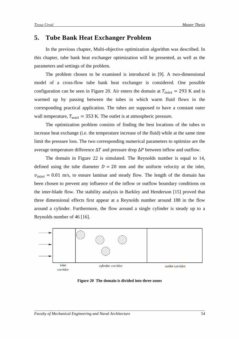
Tessa Uroić Master Thesis
5. Tube Bank Heat Exchanger Problem
In the previous chapter, Multi-objective optimization algorithm was described. In
this chapter, tube bank heat exchanger optimization will be presented, as well as the
parameters and settings of the problem.
The problem chosen to be examined is introduced in [9]. A two-dimensional
model of a cross-flow tube bank heat exchanger is considered. One possible
configuration can be seen in Figure 20. Air enters the domain at 𝑇𝑖𝑛𝑙𝑒𝑡 = 293 K and is
warmed up by passing between the tubes in which warm fluid flows in the
corresponding practical application. The tubes are supposed to have a constant outer
wall temperature, 𝑇𝑤𝑎𝑙𝑙 = 353 K. The outlet is at atmospheric pressure.
The optimization problem consists of finding the best locations of the tubes to
increase heat exchange (i.e. the temperature increase of the fluid) while at the same time
limit the pressure loss. The two corresponding numerical parameters to optimize are the
average temperature difference ∆𝑇 and pressure drop ∆𝑃 between inflow and outflow.
The domain in Figure 22 is simulated. The Reynolds number is equal to 14,
defined using the tube diameter 𝐷 = 20 mm and the uniform velocity at the inlet,
𝑣𝑖𝑛𝑙𝑒𝑡 = 0.01 m/s, to ensure laminar and steady flow. The length of the domain has
been chosen to prevent any influence of the inflow or outflow boundary conditions on
the inter-blade flow. The stability analysis in Barkley and Henderson [15] proved that
three dimensional effects first appear at a Reynolds number around 188 in the flow
around a cylinder. Furthermore, the flow around a single cylinder is steady up to a
Reynolds number of 46 [16].
Figure 20 The domain is divided into three zones
_____________________________________________________________________________________ Faculty of Mechanical Engineering and Naval Architecture 54
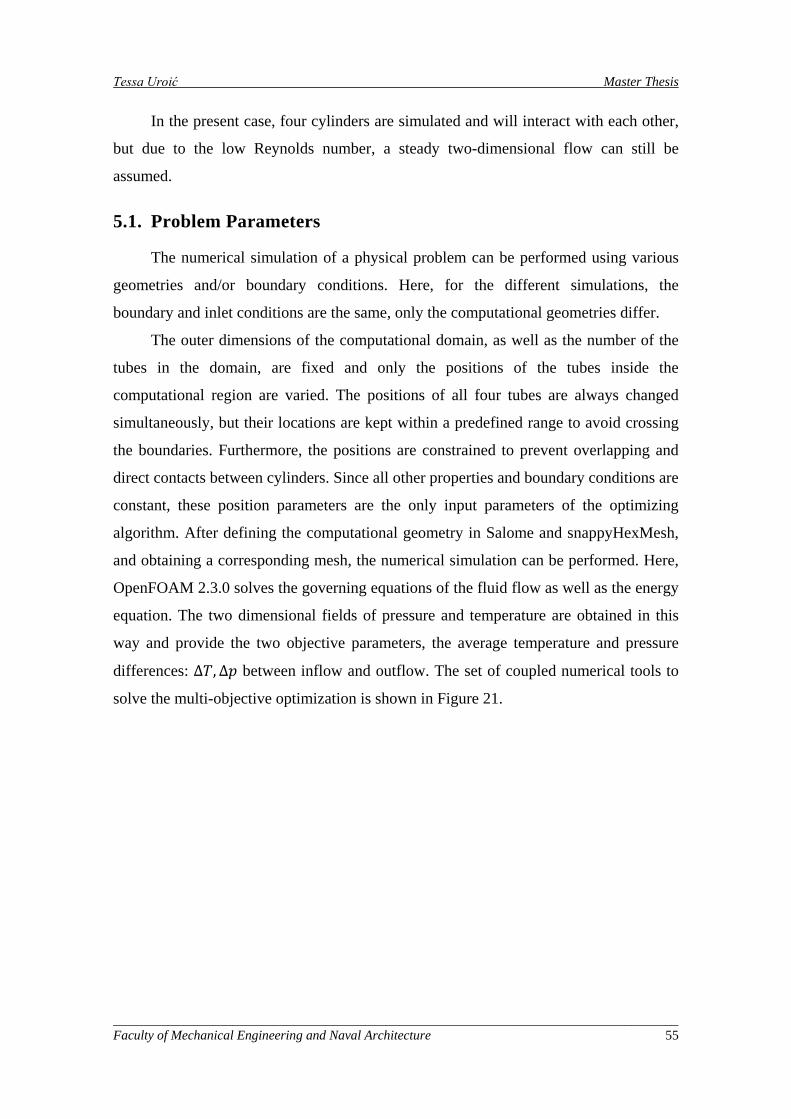
Tessa Uroić Master Thesis
In the present case, four cylinders are simulated and will interact with each other,
but due to the low Reynolds number, a steady two-dimensional flow can still be
assumed.
5.1. Problem Parameters
The numerical simulation of a physical problem can be performed using various
geometries and/or boundary conditions. Here, for the different simulations, the
boundary and inlet conditions are the same, only the computational geometries differ.
The outer dimensions of the computational domain, as well as the number of the
tubes in the domain, are fixed and only the positions of the tubes inside the
computational region are varied. The positions of all four tubes are always changed
simultaneously, but their locations are kept within a predefined range to avoid crossing
the boundaries. Furthermore, the positions are constrained to prevent overlapping and
direct contacts between cylinders. Since all other properties and boundary conditions are
constant, these position parameters are the only input parameters of the optimizing
algorithm. After defining the computational geometry in Salome and snappyHexMesh,
and obtaining a corresponding mesh, the numerical simulation can be performed. Here,
OpenFOAM 2.3.0 solves the governing equations of the fluid flow as well as the energy
equation. The two dimensional fields of pressure and temperature are obtained in this
way and provide the two objective parameters, the average temperature and pressure
differences: ∆𝑇,∆𝑝 between inflow and outflow. The set of coupled numerical tools to
solve the multi-objective optimization is shown in Figure 21.
_____________________________________________________________________________________ Faculty of Mechanical Engineering and Naval Architecture 55
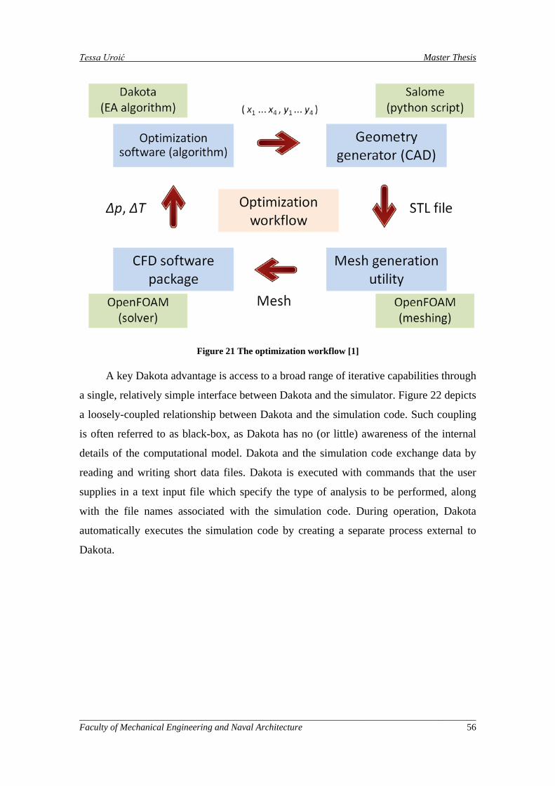
Tessa Uroić Master Thesis
Figure 21 The optimization workflow [1]
A key Dakota advantage is access to a broad range of iterative capabilities through
a single, relatively simple interface between Dakota and the simulator. Figure 22 depicts
a loosely-coupled relationship between Dakota and the simulation code. Such coupling
is often referred to as black-box, as Dakota has no (or little) awareness of the internal
details of the computational model. Dakota and the simulation code exchange data by
reading and writing short data files. Dakota is executed with commands that the user
supplies in a text input file which specify the type of analysis to be performed, along
with the file names associated with the simulation code. During operation, Dakota
automatically executes the simulation code by creating a separate process external to
Dakota.
_____________________________________________________________________________________ Faculty of Mechanical Engineering and Naval Architecture 56
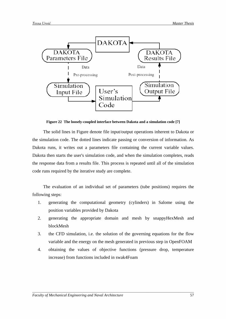
Tessa Uroić Master Thesis
Figure 22 The loosely-coupled interface between Dakota and a simulation code [7]
The solid lines in Figure denote file input/output operations inherent to Dakota or
the simulation code. The dotted lines indicate passing or conversion of information. As
Dakota runs, it writes out a parameters file containing the current variable values.
Dakota then starts the user's simulation code, and when the simulation completes, reads
the response data from a results file. This process is repeated until all of the simulation
code runs required by the iterative study are complete.
The evaluation of an individual set of parameters (tube positions) requires the
following steps:
1. generating the computational geometry (cylinders) in Salome using the
position variables provided by Dakota
2. generating the appropriate domain and mesh by snappyHexMesh and
blockMesh
3. the CFD simulation, i.e. the solution of the governing equations for the flow
variable and the energy on the mesh generated in previous step in OpenFOAM
4. obtaining the values of objective functions (pressure drop, temperature
increase) from functions included in swak4Foam
_____________________________________________________________________________________ Faculty of Mechanical Engineering and Naval Architecture 57
Tessa Uroić Master Thesis
Step 1: Computational Geometry
The geometrical constraints are prescribed in terms of lower and upper limits on
the parameters. The positions of the centers of the four cylinders (tubes) of the heat
exchanger are given with their two dimensional coordinates, 𝑥𝑖 and 𝑦𝑖, where 𝑖 =
1, 2, 3, 4. Dakota gives the coordinates to Salome which creates the cylinders. The CAD
file from Salome is delivered to snappyHexMesh where the domain is created. The
domain is separated by constraints in three non-overlapping zones in x-direction. The
first part is the inlet zone and the last one is the outlet zone. The tubes are not allowed to
be positioned in the first and last zone to prevent any interaction with the boundary
conditions, and tubes’ center coordinates have upper and lower bounds which ensure
that there are no intersections with the cyclic boundaries. The middle zone contains the
tubes. Overlapping and direct contact are not allowed. This is achieved through
constraints embedded in Dakota – collisions and overlapping are detected by checking
the minimal distance constraint. If one of the constraints is broken, after the CFD
simulation infeasible values of objective functions are assigned to these cases and they
are rejected. The radius of the tubes is 10 mm, and minimal distance was set to 21 mm,
thus the minimal allowed distance between tubes’ walls was 1 mm. The minimal
distance constraint was introduced to ensure that at least one mesh cell can fit between
the tubes. The response functions were pressure drop, temperature increase, and six
additional distance constraint functions.
Figure 23 The dimensions of the computational domain
Step 2: Mesh Generation
The initial mesh is produced by blockMesh and then snappyHexMesh includes the
cylinders delivered from Salome and refines the mesh around them. An example of the
_____________________________________________________________________________________ Faculty of Mechanical Engineering and Naval Architecture 58
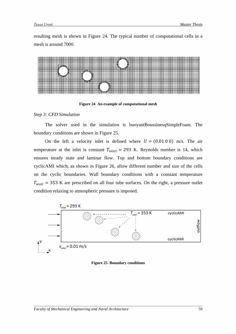
Tessa Uroić Master Thesis
resulting mesh is shown in Figure 24. The typical number of computational cells in a
mesh is around 7000.
Figure 24 An example of computational mesh
Step 3: CFD Simulation
The solver used in the simulation is buoyantBoussinesqSimpleFoam. The
boundary conditions are shown in Figure 25.
On the left a velocity inlet is defined where 𝑈 = (0.01 0 0) m/s. The air
temperature at the inlet is constant 𝑇𝑖𝑛𝑙𝑒𝑡 = 293 K. Reynolds number is 14, which
ensures steady state and laminar flow. Top and bottom boundary conditions are
cyclicAMI which, as shown in Figure 26, allow different number and size of the cells
on the cyclic boundaries. Wall boundary conditions with a constant temperature
𝑇𝑤𝑎𝑙𝑙 = 353 K are prescribed on all four tube surfaces. On the right, a pressure outlet
condition relaxing to atmospheric pressure is imposed.
Figure 25 Boundary conditions
_____________________________________________________________________________________ Faculty of Mechanical Engineering and Naval Architecture 59
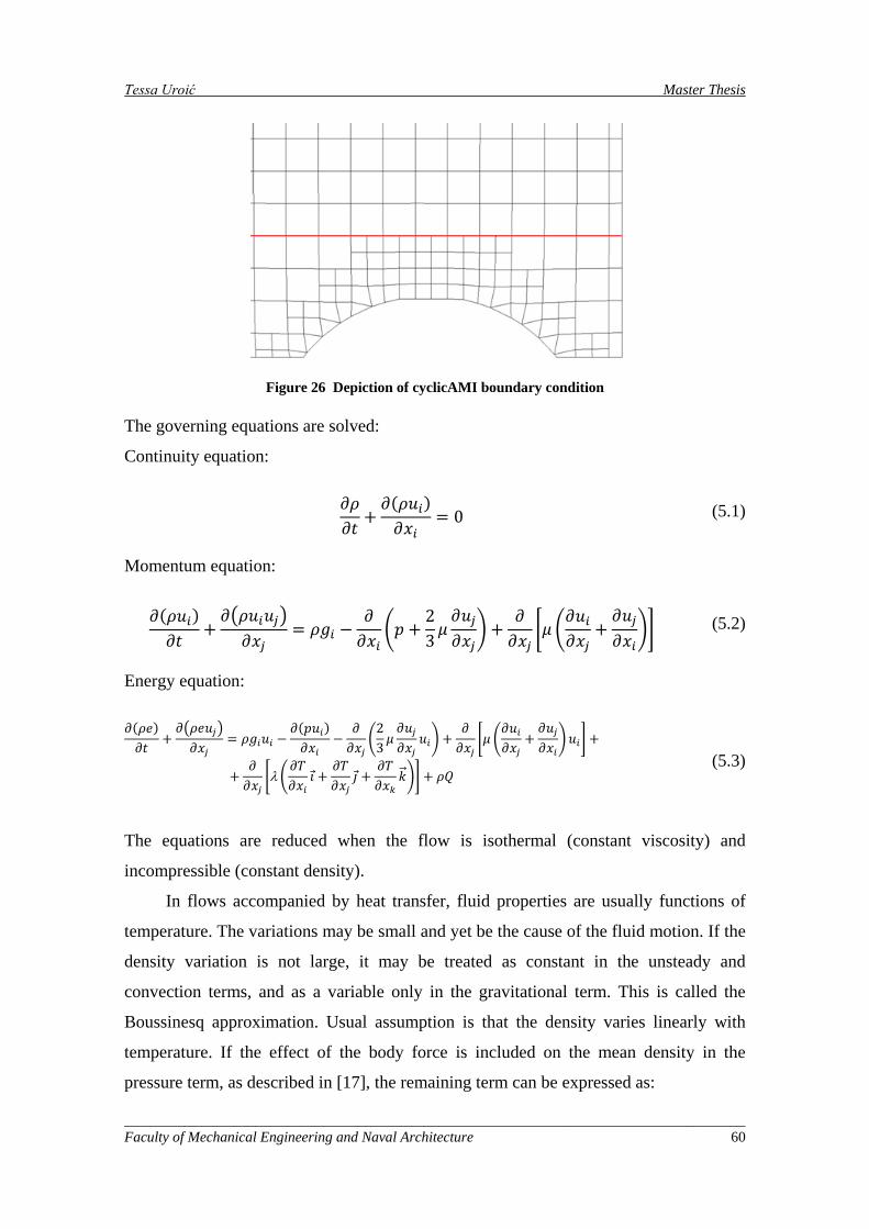
Tessa Uroić Master Thesis
Figure 26 Depiction of cyclicAMI boundary condition
The governing equations are solved:
Continuity equation:
𝜕𝜌𝜕𝑡
+𝜕(𝜌𝑢𝑖)𝜕𝑥𝑖
= 0 (5.1)
Momentum equation:
𝜕(𝜌𝑢𝑖)𝜕𝑡
+𝜕�𝜌𝑢𝑖𝑢𝑗�𝜕𝑥𝑗
= 𝜌𝑔𝑖 −𝜕𝜕𝑥𝑖
�𝑝 +23𝜇𝜕𝑢𝑗𝜕𝑥𝑗
� +𝜕𝜕𝑥𝑗
�𝜇 �𝜕𝑢𝑖𝜕𝑥𝑗
+𝜕𝑢𝑗𝜕𝑥𝑖
�� (5.2)
Energy equation:
𝜕(𝜌𝑒)𝜕𝑡
+𝜕�𝜌𝑒𝑢𝑗�𝜕𝑥𝑗
= 𝜌𝑔𝑖𝑢𝑖 −𝜕(𝑝𝑢𝑖)𝜕𝑥𝑖
−𝜕𝜕𝑥𝑗
�23𝜇𝜕𝑢𝑗𝜕𝑥𝑗
𝑢𝑖� +𝜕𝜕𝑥𝑗
�𝜇 �𝜕𝑢𝑖𝜕𝑥𝑗
+𝜕𝑢𝑗𝜕𝑥𝑖
� 𝑢𝑖� + +
+𝜕𝜕𝑥𝑗
�λ�𝜕𝑇𝜕𝑥𝑖
𝚤 +𝜕𝑇𝜕𝑥𝑗
𝚥 +𝜕𝑇𝜕𝑥𝑘
𝑘�⃗ �� + 𝜌𝑄 (5.3)
The equations are reduced when the flow is isothermal (constant viscosity) and
incompressible (constant density).
In flows accompanied by heat transfer, fluid properties are usually functions of
temperature. The variations may be small and yet be the cause of the fluid motion. If the
density variation is not large, it may be treated as constant in the unsteady and
convection terms, and as a variable only in the gravitational term. This is called the
Boussinesq approximation. Usual assumption is that the density varies linearly with
temperature. If the effect of the body force is included on the mean density in the
pressure term, as described in [17], the remaining term can be expressed as:
_____________________________________________________________________________________ Faculty of Mechanical Engineering and Naval Architecture 60
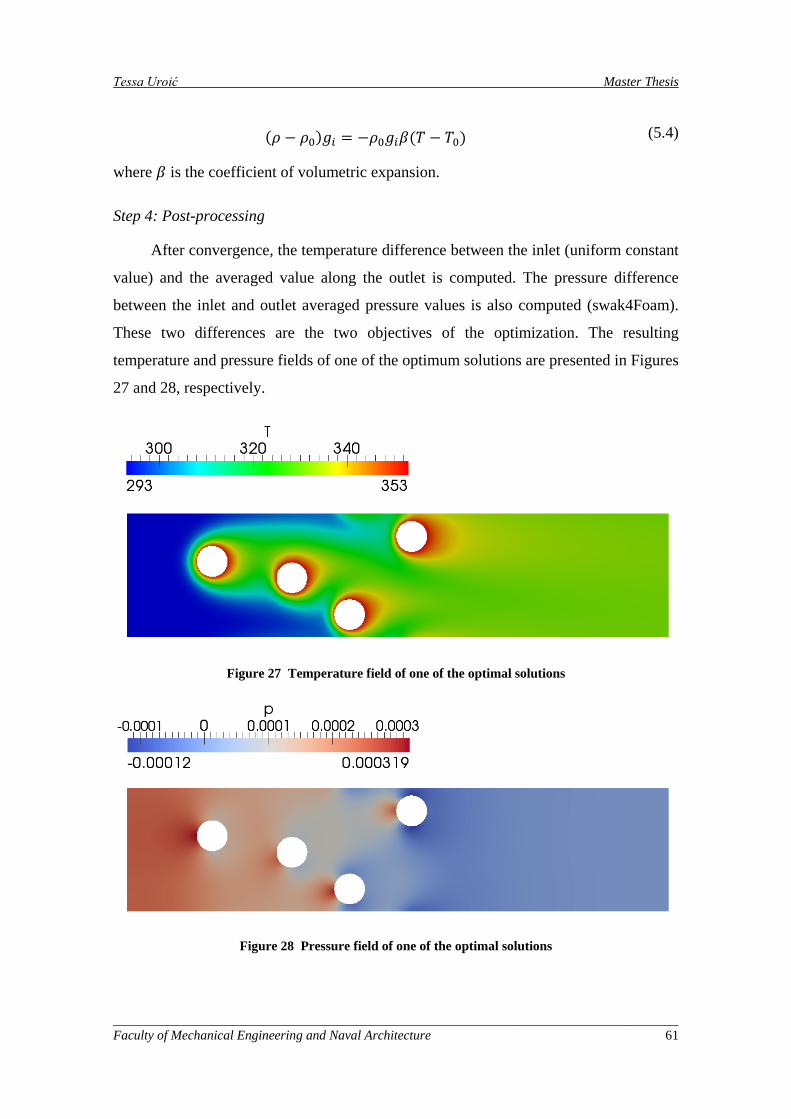
Tessa Uroić Master Thesis
(𝜌 − 𝜌0)𝑔𝑖 = −𝜌0𝑔𝑖𝛽(𝑇 − 𝑇0) (5.4)
where 𝛽 is the coefficient of volumetric expansion.
Step 4: Post-processing
After convergence, the temperature difference between the inlet (uniform constant
value) and the averaged value along the outlet is computed. The pressure difference
between the inlet and outlet averaged pressure values is also computed (swak4Foam).
These two differences are the two objectives of the optimization. The resulting
temperature and pressure fields of one of the optimum solutions are presented in Figures
27 and 28, respectively.
Figure 27 Temperature field of one of the optimal solutions
Figure 28 Pressure field of one of the optimal solutions
_____________________________________________________________________________________ Faculty of Mechanical Engineering and Naval Architecture 61

Tessa Uroić Master Thesis
In this chapter, parameters and settings of the tube bank heat exchanger problem
were presented. In the next chapter, results of the optimization and uncertainty
quantification will be presented and discussed.
_____________________________________________________________________________________ Faculty of Mechanical Engineering and Naval Architecture 62
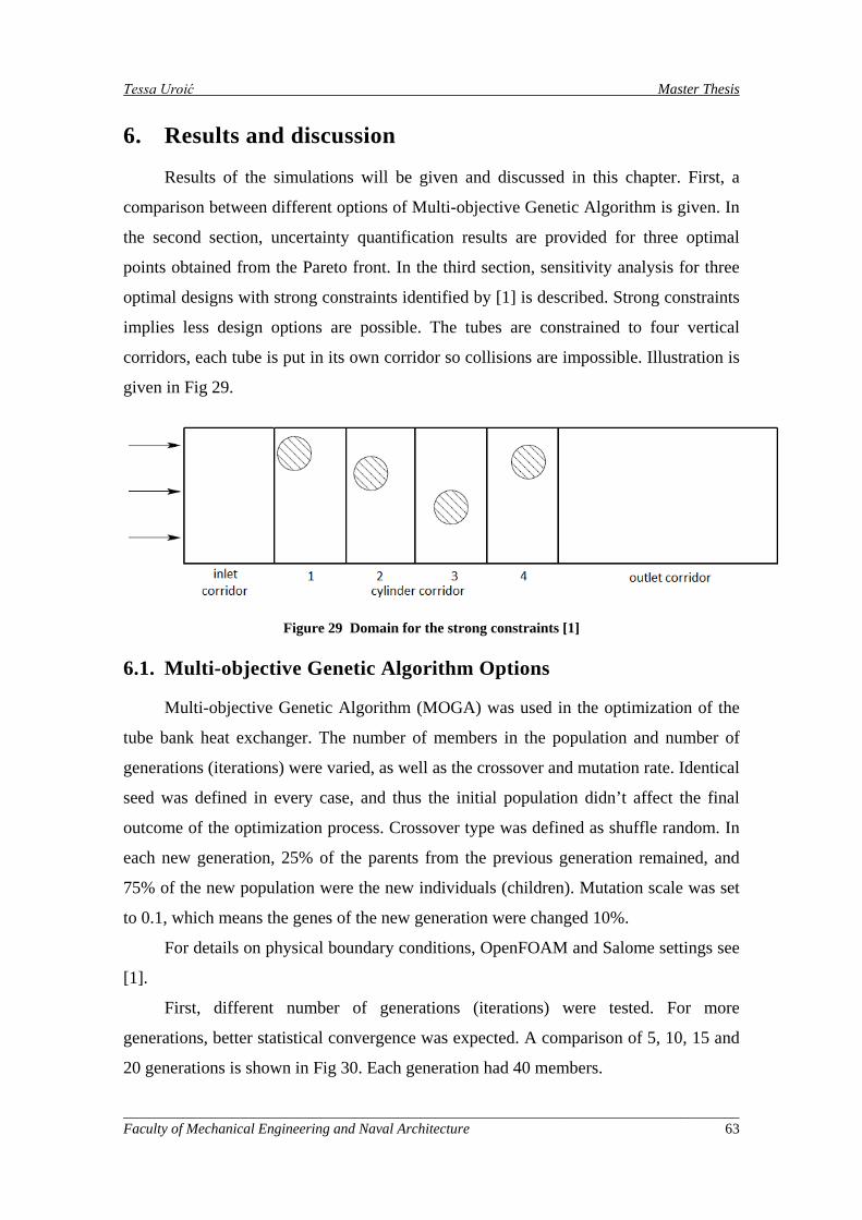
Tessa Uroić Master Thesis
6. Results and discussion
Results of the simulations will be given and discussed in this chapter. First, a
comparison between different options of Multi-objective Genetic Algorithm is given. In
the second section, uncertainty quantification results are provided for three optimal
points obtained from the Pareto front. In the third section, sensitivity analysis for three
optimal designs with strong constraints identified by [1] is described. Strong constraints
implies less design options are possible. The tubes are constrained to four vertical
corridors, each tube is put in its own corridor so collisions are impossible. Illustration is
given in Fig 29.
Figure 29 Domain for the strong constraints [1]
6.1. Multi-objective Genetic Algorithm Options
Multi-objective Genetic Algorithm (MOGA) was used in the optimization of the
tube bank heat exchanger. The number of members in the population and number of
generations (iterations) were varied, as well as the crossover and mutation rate. Identical
seed was defined in every case, and thus the initial population didn’t affect the final
outcome of the optimization process. Crossover type was defined as shuffle random. In
each new generation, 25% of the parents from the previous generation remained, and
75% of the new population were the new individuals (children). Mutation scale was set
to 0.1, which means the genes of the new generation were changed 10%.
For details on physical boundary conditions, OpenFOAM and Salome settings see
[1].
First, different number of generations (iterations) were tested. For more
generations, better statistical convergence was expected. A comparison of 5, 10, 15 and
20 generations is shown in Fig 30. Each generation had 40 members.
_____________________________________________________________________________________ Faculty of Mechanical Engineering and Naval Architecture 63
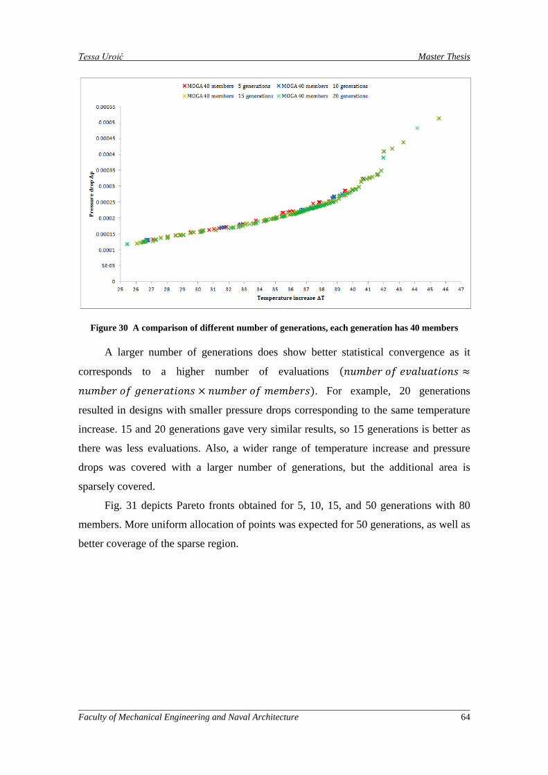
Tessa Uroić Master Thesis
Figure 30 A comparison of different number of generations, each generation has 40 members
A larger number of generations does show better statistical convergence as it
corresponds to a higher number of evaluations (𝑛𝑢𝑚𝑏𝑒𝑟 𝑜𝑓 𝑒𝑣𝑎𝑙𝑢𝑎𝑡𝑖𝑜𝑛𝑠 ≈
𝑛𝑢𝑚𝑏𝑒𝑟 𝑜𝑓 𝑔𝑒𝑛𝑒𝑟𝑎𝑡𝑖𝑜𝑛𝑠 × 𝑛𝑢𝑚𝑏𝑒𝑟 𝑜𝑓 𝑚𝑒𝑚𝑏𝑒𝑟𝑠). For example, 20 generations
resulted in designs with smaller pressure drops corresponding to the same temperature
increase. 15 and 20 generations gave very similar results, so 15 generations is better as
there was less evaluations. Also, a wider range of temperature increase and pressure
drops was covered with a larger number of generations, but the additional area is
sparsely covered.
Fig. 31 depicts Pareto fronts obtained for 5, 10, 15, and 50 generations with 80
members. More uniform allocation of points was expected for 50 generations, as well as
better coverage of the sparse region.
_____________________________________________________________________________________ Faculty of Mechanical Engineering and Naval Architecture 64
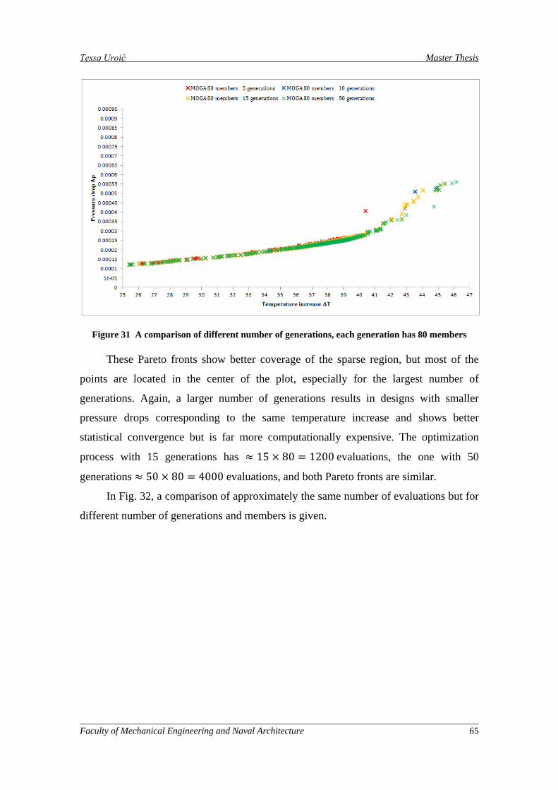
Tessa Uroić Master Thesis
Figure 31 A comparison of different number of generations, each generation has 80 members
These Pareto fronts show better coverage of the sparse region, but most of the
points are located in the center of the plot, especially for the largest number of
generations. Again, a larger number of generations results in designs with smaller
pressure drops corresponding to the same temperature increase and shows better
statistical convergence but is far more computationally expensive. The optimization
process with 15 generations has ≈ 15 × 80 = 1200 evaluations, the one with 50
generations ≈ 50 × 80 = 4000 evaluations, and both Pareto fronts are similar.
In Fig. 32, a comparison of approximately the same number of evaluations but for
different number of generations and members is given.
_____________________________________________________________________________________ Faculty of Mechanical Engineering and Naval Architecture 65
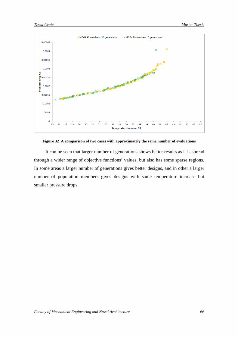
Tessa Uroić Master Thesis
Figure 32 A comparison of two cases with approximately the same number of evaluations
It can be seen that larger number of generations shows better results as it is spread
through a wider range of objective functions’ values, but also has some sparse regions.
In some areas a larger number of generations gives better designs, and in other a larger
number of population members gives designs with same temperature increase but
smaller pressure drops.
_____________________________________________________________________________________ Faculty of Mechanical Engineering and Naval Architecture 66
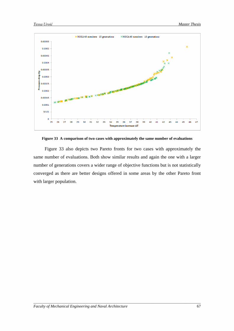
Tessa Uroić Master Thesis
Figure 33 A comparison of two cases with approximately the same number of evaluations
Figure 33 also depicts two Pareto fronts for two cases with approximately the
same number of evaluations. Both show similar results and again the one with a larger
number of generations covers a wider range of objective functions but is not statistically
converged as there are better designs offered in some areas by the other Pareto front
with larger population.
_____________________________________________________________________________________ Faculty of Mechanical Engineering and Naval Architecture 67
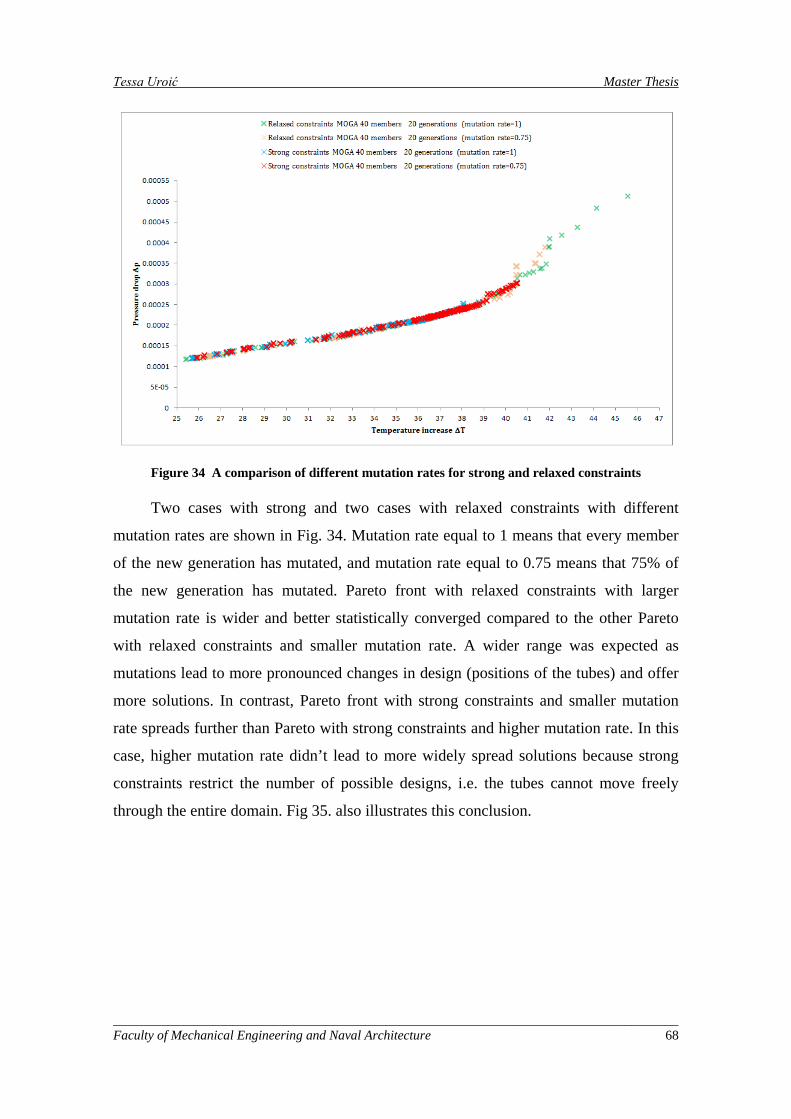
Tessa Uroić Master Thesis
Figure 34 A comparison of different mutation rates for strong and relaxed constraints
Two cases with strong and two cases with relaxed constraints with different
mutation rates are shown in Fig. 34. Mutation rate equal to 1 means that every member
of the new generation has mutated, and mutation rate equal to 0.75 means that 75% of
the new generation has mutated. Pareto front with relaxed constraints with larger
mutation rate is wider and better statistically converged compared to the other Pareto
with relaxed constraints and smaller mutation rate. A wider range was expected as
mutations lead to more pronounced changes in design (positions of the tubes) and offer
more solutions. In contrast, Pareto front with strong constraints and smaller mutation
rate spreads further than Pareto with strong constraints and higher mutation rate. In this
case, higher mutation rate didn’t lead to more widely spread solutions because strong
constraints restrict the number of possible designs, i.e. the tubes cannot move freely
through the entire domain. Fig 35. also illustrates this conclusion.
_____________________________________________________________________________________ Faculty of Mechanical Engineering and Naval Architecture 68
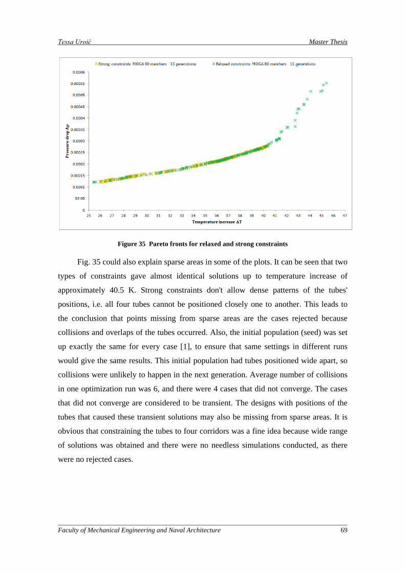
Tessa Uroić Master Thesis
Figure 35 Pareto fronts for relaxed and strong constraints
Fig. 35 could also explain sparse areas in some of the plots. It can be seen that two
types of constraints gave almost identical solutions up to temperature increase of
approximately 40.5 K. Strong constraints don't allow dense patterns of the tubes'
positions, i.e. all four tubes cannot be positioned closely one to another. This leads to
the conclusion that points missing from sparse areas are the cases rejected because
collisions and overlaps of the tubes occurred. Also, the initial population (seed) was set
up exactly the same for every case [1], to ensure that same settings in different runs
would give the same results. This initial population had tubes positioned wide apart, so
collisions were unlikely to happen in the next generation. Average number of collisions
in one optimization run was 6, and there were 4 cases that did not converge. The cases
that did not converge are considered to be transient. The designs with positions of the
tubes that caused these transient solutions may also be missing from sparse areas. It is
obvious that constraining the tubes to four corridors was a fine idea because wide range
of solutions was obtained and there were no needless simulations conducted, as there
were no rejected cases.
_____________________________________________________________________________________ Faculty of Mechanical Engineering and Naval Architecture 69
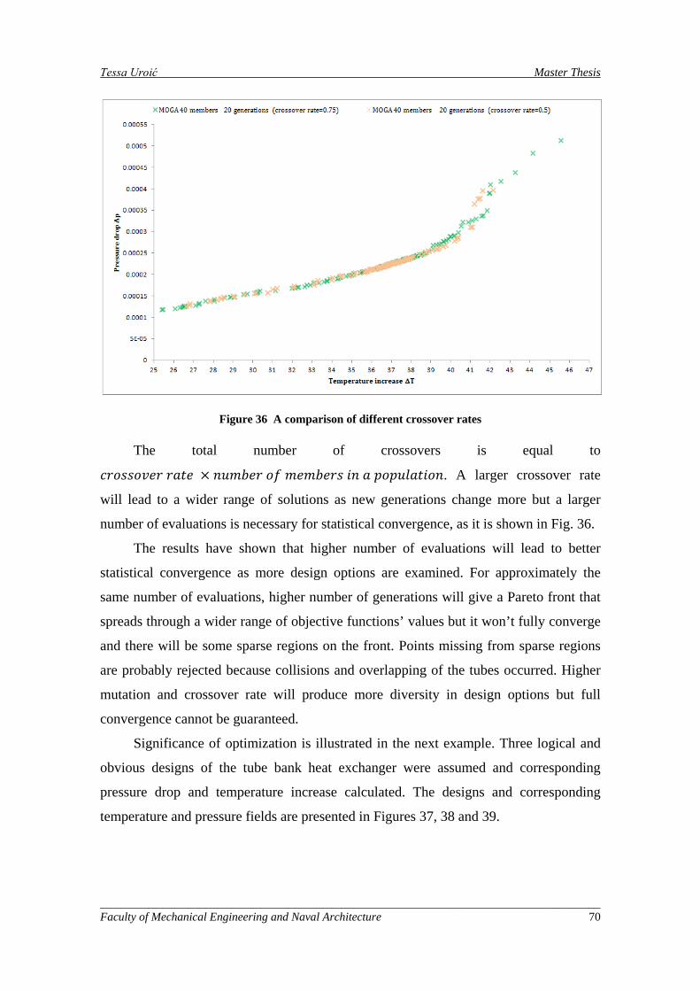
Tessa Uroić Master Thesis
Figure 36 A comparison of different crossover rates
The total number of crossovers is equal to
𝑐𝑟𝑜𝑠𝑠𝑜𝑣𝑒𝑟 𝑟𝑎𝑡𝑒 × 𝑛𝑢𝑚𝑏𝑒𝑟 𝑜𝑓 𝑚𝑒𝑚𝑏𝑒𝑟𝑠 𝑖𝑛 𝑎 𝑝𝑜𝑝𝑢𝑙𝑎𝑡𝑖𝑜𝑛. A larger crossover rate
will lead to a wider range of solutions as new generations change more but a larger
number of evaluations is necessary for statistical convergence, as it is shown in Fig. 36.
The results have shown that higher number of evaluations will lead to better
statistical convergence as more design options are examined. For approximately the
same number of evaluations, higher number of generations will give a Pareto front that
spreads through a wider range of objective functions’ values but it won’t fully converge
and there will be some sparse regions on the front. Points missing from sparse regions
are probably rejected because collisions and overlapping of the tubes occurred. Higher
mutation and crossover rate will produce more diversity in design options but full
convergence cannot be guaranteed.
Significance of optimization is illustrated in the next example. Three logical and
obvious designs of the tube bank heat exchanger were assumed and corresponding
pressure drop and temperature increase calculated. The designs and corresponding
temperature and pressure fields are presented in Figures 37, 38 and 39.
_____________________________________________________________________________________ Faculty of Mechanical Engineering and Naval Architecture 70
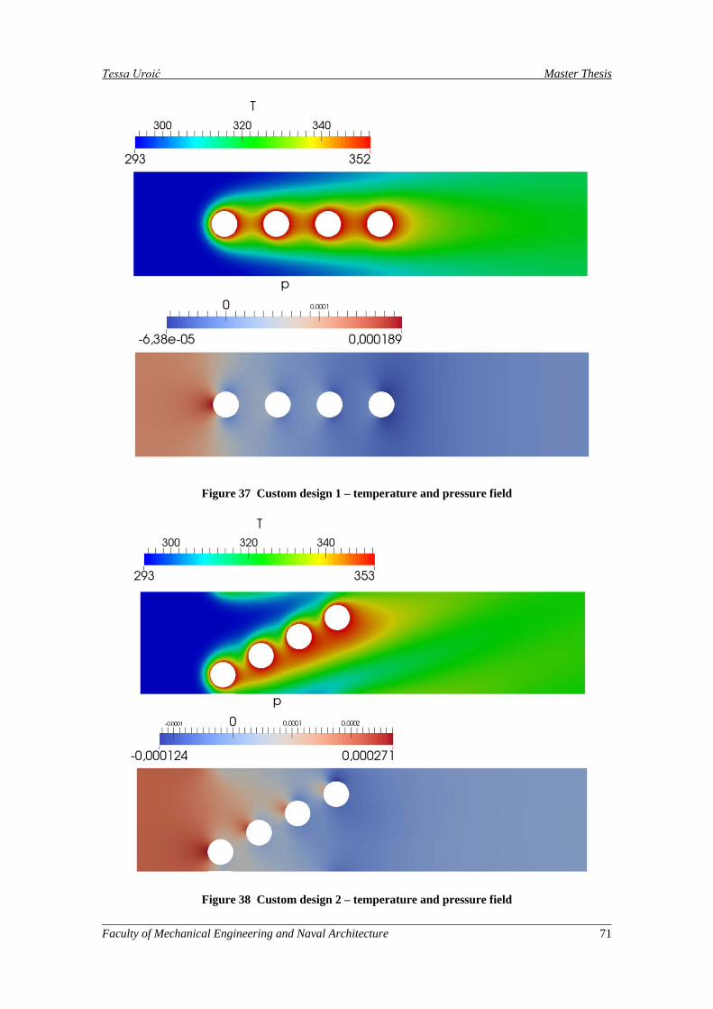
Tessa Uroić Master Thesis
Figure 37 Custom design 1 – temperature and pressure field
Figure 38 Custom design 2 – temperature and pressure field
_____________________________________________________________________________________ Faculty of Mechanical Engineering and Naval Architecture 71

Tessa Uroić Master Thesis
Figure 39 Custom design 3 – temperature and pressure field
The tubes are lined up horizontally one behind the other in the first case, so very
low pressure drop is expected. In the second case, they are lined up diagonally and
higher pressure drop is expected, but also temperature increase. In the third case, the
pattern of the tubes’ positions is criss-cross, and higher pressure drop than design 1 is
expected, as well as higher temperature increase. The positions of the corresponding
points in objective function space for each of the three custom designs are shown in
Figure 40.
_____________________________________________________________________________________ Faculty of Mechanical Engineering and Naval Architecture 72
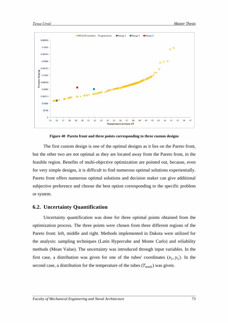
Tessa Uroić Master Thesis
Figure 40 Pareto front and three points corresponding to three custom designs
The first custom design is one of the optimal designs as it lies on the Pareto front,
but the other two are not optimal as they are located away from the Pareto front, in the
feasible region. Benefits of multi-objective optimization are pointed out, because, even
for very simple designs, it is difficult to find numerous optimal solutions experientially.
Pareto front offers numerous optimal solutions and decision maker can give additional
subjective preference and choose the best option corresponding to the specific problem
or system.
6.2. Uncertainty Quantification
Uncertainty quantification was done for three optimal points obtained from the
optimization process. The three points were chosen from three different regions of the
Pareto front: left, middle and right. Methods implemented in Dakota were utilized for
the analysis: sampling techniques (Latin Hypercube and Monte Carlo) and reliability
methods (Mean Value). The uncertainty was introduced through input variables. In the
first case, a distribution was given for one of the tubes' coordinates (𝑥1,𝑦1). In the
second case, a distribution for the temperature of the tubes (𝑇𝑤𝑎𝑙𝑙) was given.
_____________________________________________________________________________________ Faculty of Mechanical Engineering and Naval Architecture 73
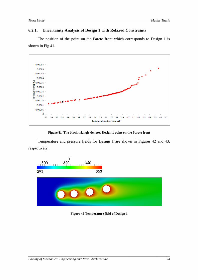
Tessa Uroić Master Thesis
6.2.1. Uncertainty Analysis of Design 1 with Relaxed Constraints
The position of the point on the Pareto front which corresponds to Design 1 is
shown in Fig 41.
Figure 41 The black triangle denotes Design 1 point on the Pareto front
Temperature and pressure fields for Design 1 are shown in Figures 42 and 43,
respectively.
Figure 42 Temperature field of Design 1
_____________________________________________________________________________________ Faculty of Mechanical Engineering and Naval Architecture 74
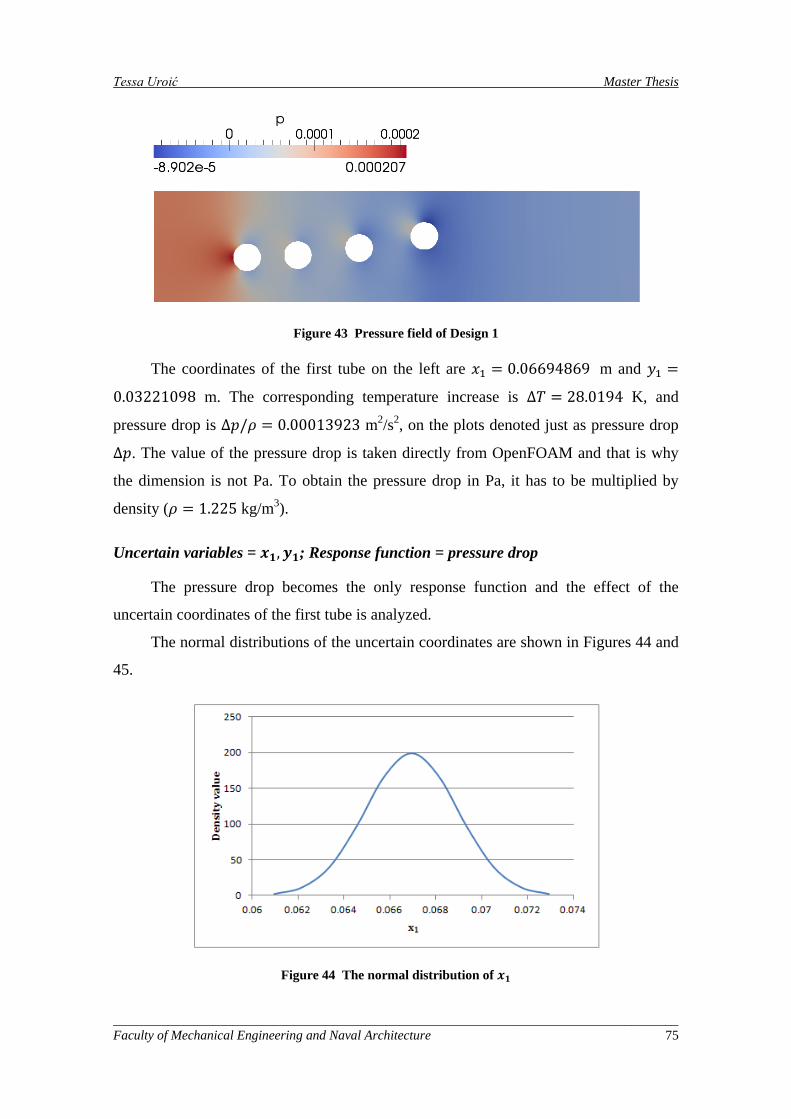
Tessa Uroić Master Thesis
Figure 43 Pressure field of Design 1
The coordinates of the first tube on the left are 𝑥1 = 0.06694869 m and 𝑦1 =
0.03221098 m. The corresponding temperature increase is ∆𝑇 = 28.0194 K, and
pressure drop is ∆𝑝/𝜌 = 0.00013923 m2/s2, on the plots denoted just as pressure drop
∆𝑝. The value of the pressure drop is taken directly from OpenFOAM and that is why
the dimension is not Pa. To obtain the pressure drop in Pa, it has to be multiplied by
density (𝜌 = 1.225 kg/m3).
Uncertain variables = 𝒙𝟏,𝒚𝟏; Response function = pressure drop
The pressure drop becomes the only response function and the effect of the
uncertain coordinates of the first tube is analyzed.
The normal distributions of the uncertain coordinates are shown in Figures 44 and
45.
Figure 44 The normal distribution of 𝒙𝟏
_____________________________________________________________________________________ Faculty of Mechanical Engineering and Naval Architecture 75
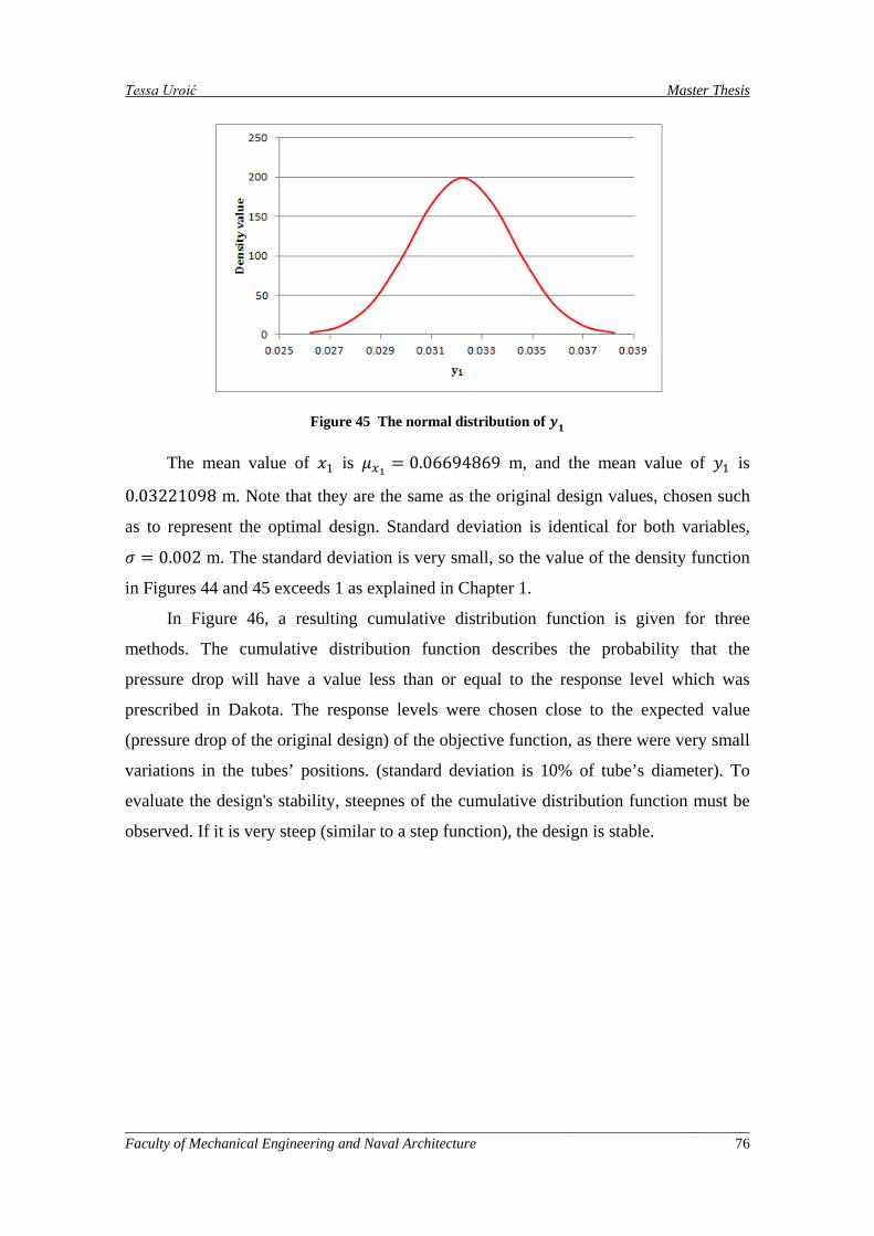
Tessa Uroić Master Thesis
Figure 45 The normal distribution of 𝒚𝟏
The mean value of 𝑥1 is 𝜇𝑥1 = 0.06694869 m, and the mean value of 𝑦1 is
0.03221098 m. Note that they are the same as the original design values, chosen such
as to represent the optimal design. Standard deviation is identical for both variables,
𝜎 = 0.002 m. The standard deviation is very small, so the value of the density function
in Figures 44 and 45 exceeds 1 as explained in Chapter 1.
In Figure 46, a resulting cumulative distribution function is given for three
methods. The cumulative distribution function describes the probability that the
pressure drop will have a value less than or equal to the response level which was
prescribed in Dakota. The response levels were chosen close to the expected value
(pressure drop of the original design) of the objective function, as there were very small
variations in the tubes’ positions. (standard deviation is 10% of tube’s diameter). To
evaluate the design's stability, steepnes of the cumulative distribution function must be
observed. If it is very steep (similar to a step function), the design is stable.
_____________________________________________________________________________________ Faculty of Mechanical Engineering and Naval Architecture 76
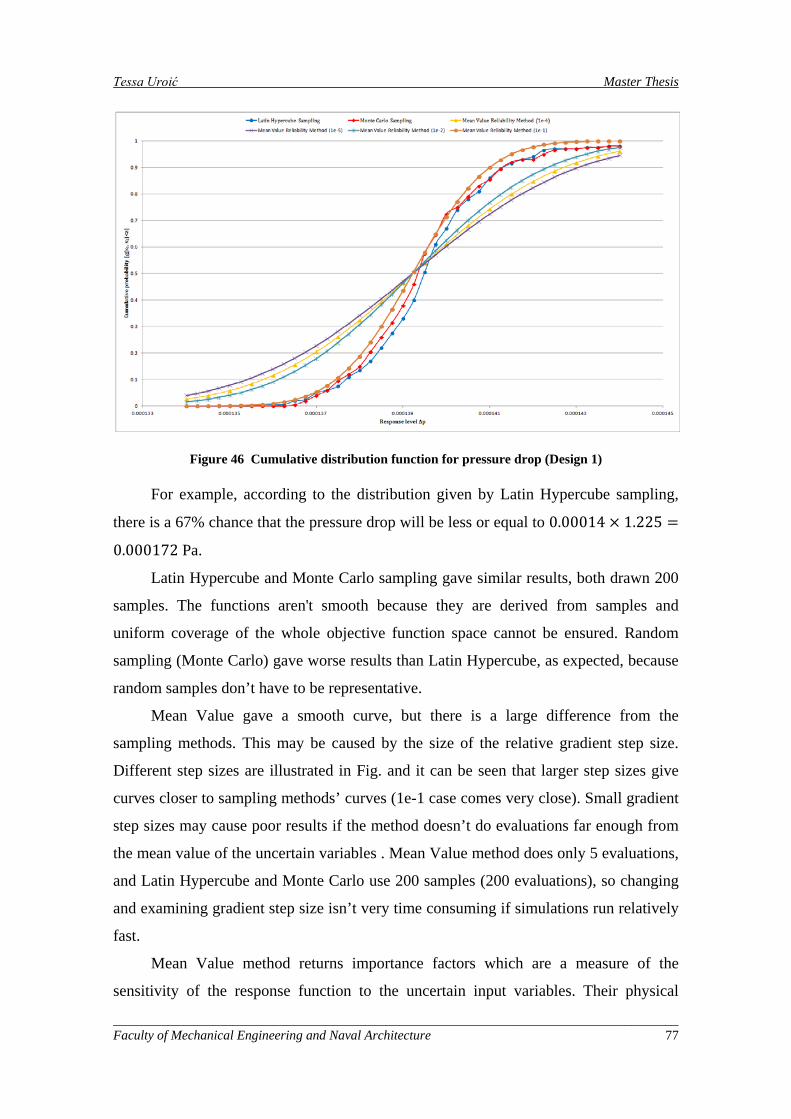
Tessa Uroić Master Thesis
Figure 46 Cumulative distribution function for pressure drop (Design 1)
For example, according to the distribution given by Latin Hypercube sampling,
there is a 67% chance that the pressure drop will be less or equal to 0.00014 × 1.225 =
0.000172 Pa.
Latin Hypercube and Monte Carlo sampling gave similar results, both drawn 200
samples. The functions aren't smooth because they are derived from samples and
uniform coverage of the whole objective function space cannot be ensured. Random
sampling (Monte Carlo) gave worse results than Latin Hypercube, as expected, because
random samples don’t have to be representative.
Mean Value gave a smooth curve, but there is a large difference from the
sampling methods. This may be caused by the size of the relative gradient step size.
Different step sizes are illustrated in Fig. and it can be seen that larger step sizes give
curves closer to sampling methods’ curves (1e-1 case comes very close). Small gradient
step sizes may cause poor results if the method doesn’t do evaluations far enough from
the mean value of the uncertain variables . Mean Value method does only 5 evaluations,
and Latin Hypercube and Monte Carlo use 200 samples (200 evaluations), so changing
and examining gradient step size isn’t very time consuming if simulations run relatively
fast.
Mean Value method returns importance factors which are a measure of the
sensitivity of the response function to the uncertain input variables. Their physical
_____________________________________________________________________________________ Faculty of Mechanical Engineering and Naval Architecture 77
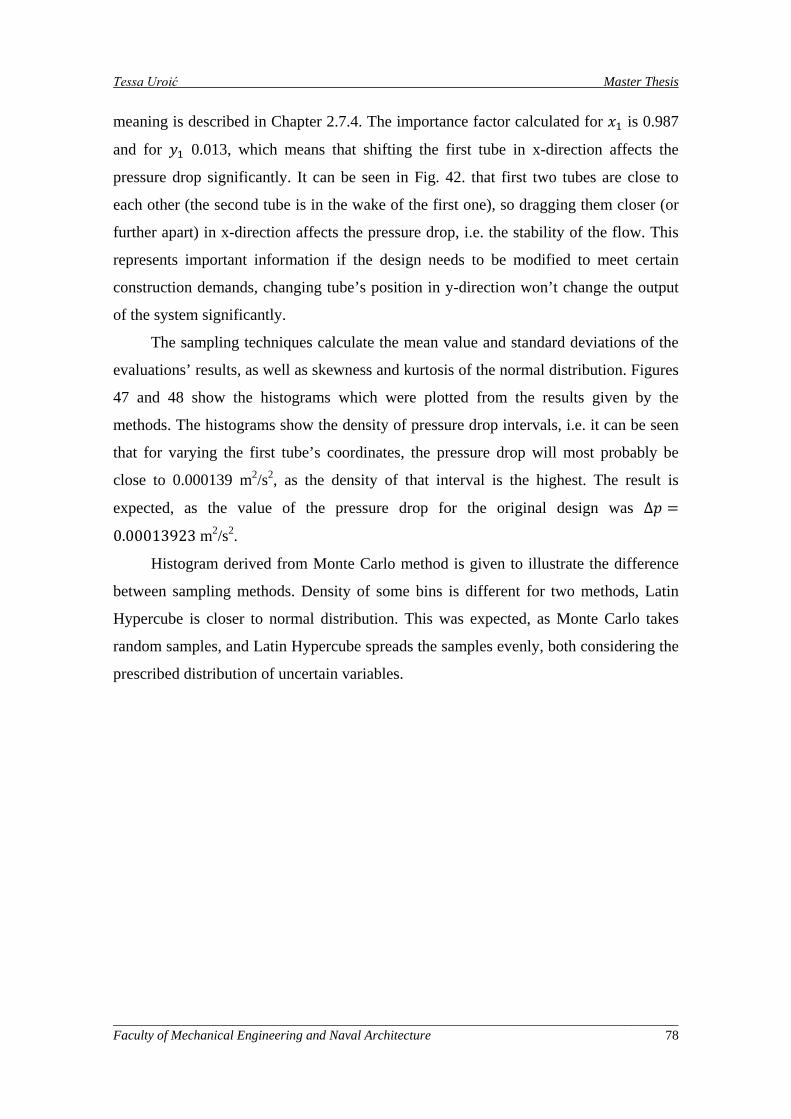
Tessa Uroić Master Thesis
meaning is described in Chapter 2.7.4. The importance factor calculated for 𝑥1 is 0.987
and for 𝑦1 0.013, which means that shifting the first tube in x-direction affects the
pressure drop significantly. It can be seen in Fig. 42. that first two tubes are close to
each other (the second tube is in the wake of the first one), so dragging them closer (or
further apart) in x-direction affects the pressure drop, i.e. the stability of the flow. This
represents important information if the design needs to be modified to meet certain
construction demands, changing tube’s position in y-direction won’t change the output
of the system significantly.
The sampling techniques calculate the mean value and standard deviations of the
evaluations’ results, as well as skewness and kurtosis of the normal distribution. Figures
47 and 48 show the histograms which were plotted from the results given by the
methods. The histograms show the density of pressure drop intervals, i.e. it can be seen
that for varying the first tube’s coordinates, the pressure drop will most probably be
close to 0.000139 m2/s2, as the density of that interval is the highest. The result is
expected, as the value of the pressure drop for the original design was ∆𝑝 =
0.00013923 m2/s2.
Histogram derived from Monte Carlo method is given to illustrate the difference
between sampling methods. Density of some bins is different for two methods, Latin
Hypercube is closer to normal distribution. This was expected, as Monte Carlo takes
random samples, and Latin Hypercube spreads the samples evenly, both considering the
prescribed distribution of uncertain variables.
_____________________________________________________________________________________ Faculty of Mechanical Engineering and Naval Architecture 78
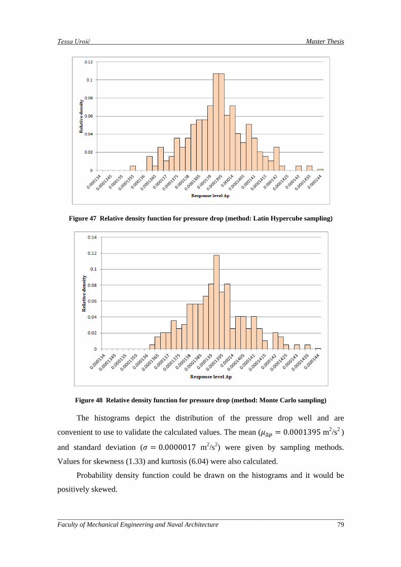
Tessa Uroić Master Thesis
Figure 47 Relative density function for pressure drop (method: Latin Hypercube sampling)
Figure 48 Relative density function for pressure drop (method: Monte Carlo sampling)
The histograms depict the distribution of the pressure drop well and are
convenient to use to validate the calculated values. The mean (𝜇∆𝑝 = 0.0001395 m2/s2 )
and standard deviation (𝜎 = 0.0000017 m2/s2) were given by sampling methods.
Values for skewness (1.33) and kurtosis (6.04) were also calculated.
Probability density function could be drawn on the histograms and it would be
positively skewed.
_____________________________________________________________________________________ Faculty of Mechanical Engineering and Naval Architecture 79
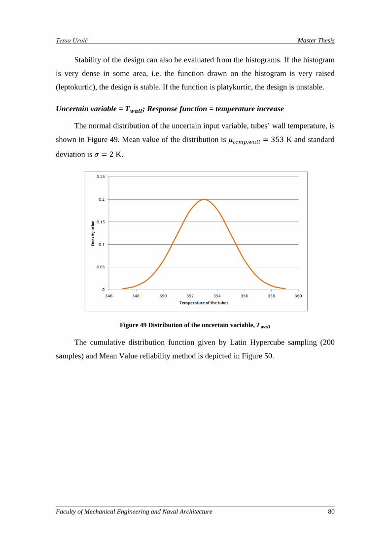
Tessa Uroić Master Thesis
Stability of the design can also be evaluated from the histograms. If the histogram
is very dense in some area, i.e. the function drawn on the histogram is very raised
(leptokurtic), the design is stable. If the function is platykurtic, the design is unstable.
Uncertain variable = 𝑻𝒘𝒂𝒍𝒍; Response function = temperature increase
The normal distribution of the uncertain input variable, tubes’ wall temperature, is
shown in Figure 49. Mean value of the distribution is 𝜇𝑡𝑒𝑚𝑝,𝑤𝑎𝑙𝑙 = 353 K and standard
deviation is 𝜎 = 2 K.
Figure 49 Distribution of the uncertain variable, 𝑻𝒘𝒂𝒍𝒍
The cumulative distribution function given by Latin Hypercube sampling (200
samples) and Mean Value reliability method is depicted in Figure 50.
_____________________________________________________________________________________ Faculty of Mechanical Engineering and Naval Architecture 80
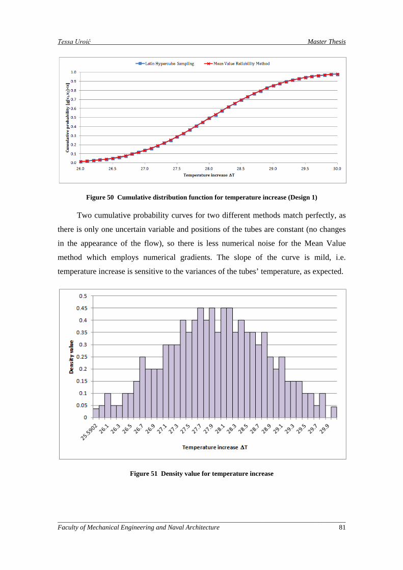
Tessa Uroić Master Thesis
Figure 50 Cumulative distribution function for temperature increase (Design 1)
Two cumulative probability curves for two different methods match perfectly, as
there is only one uncertain variable and positions of the tubes are constant (no changes
in the appearance of the flow), so there is less numerical noise for the Mean Value
method which employs numerical gradients. The slope of the curve is mild, i.e.
temperature increase is sensitive to the variances of the tubes’ temperature, as expected.
Figure 51 Density value for temperature increase
_____________________________________________________________________________________ Faculty of Mechanical Engineering and Naval Architecture 81
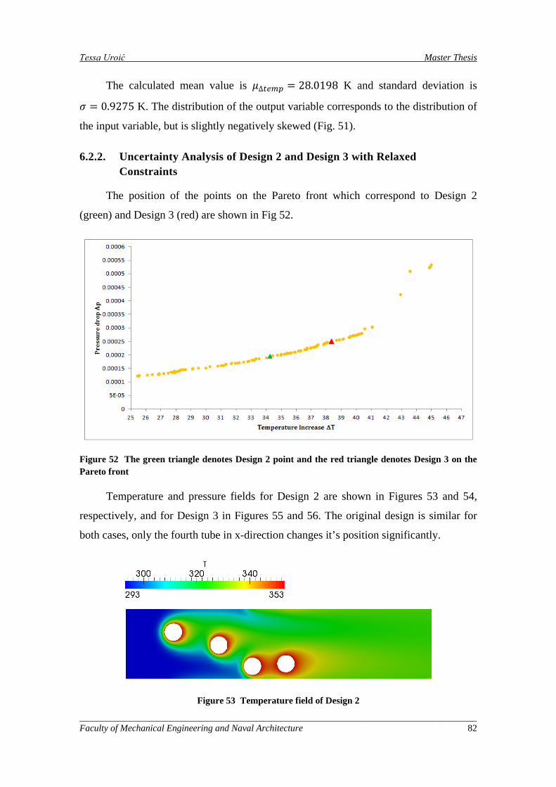
Tessa Uroić Master Thesis
The calculated mean value is 𝜇∆𝑡𝑒𝑚𝑝 = 28.0198 K and standard deviation is
𝜎 = 0.9275 K. The distribution of the output variable corresponds to the distribution of
the input variable, but is slightly negatively skewed (Fig. 51).
6.2.2. Uncertainty Analysis of Design 2 and Design 3 with Relaxed Constraints
The position of the points on the Pareto front which correspond to Design 2
(green) and Design 3 (red) are shown in Fig 52.
Figure 52 The green triangle denotes Design 2 point and the red triangle denotes Design 3 on the Pareto front
Temperature and pressure fields for Design 2 are shown in Figures 53 and 54,
respectively, and for Design 3 in Figures 55 and 56. The original design is similar for
both cases, only the fourth tube in x-direction changes it’s position significantly.
Figure 53 Temperature field of Design 2
_____________________________________________________________________________________ Faculty of Mechanical Engineering and Naval Architecture 82
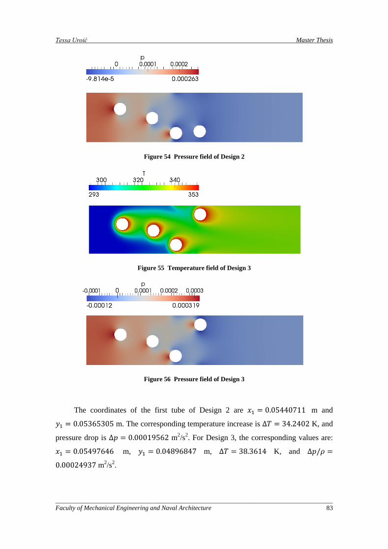
Tessa Uroić Master Thesis
Figure 54 Pressure field of Design 2
Figure 55 Temperature field of Design 3
Figure 56 Pressure field of Design 3
The coordinates of the first tube of Design 2 are 𝑥1 = 0.05440711 m and
𝑦1 = 0.05365305 m. The corresponding temperature increase is ∆𝑇 = 34.2402 K, and
pressure drop is ∆𝑝 = 0.00019562 m2/s2. For Design 3, the corresponding values are:
𝑥1 = 0.05497646 m, 𝑦1 = 0.04896847 m, ∆𝑇 = 38.3614 K, and ∆𝑝/𝜌 =
0.00024937 m2/s2.
_____________________________________________________________________________________ Faculty of Mechanical Engineering and Naval Architecture 83
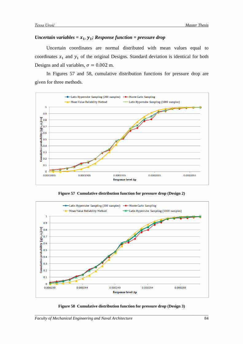
Tessa Uroić Master Thesis
Uncertain variables = 𝒙𝟏,𝒚𝟏; Response function = pressure drop
Uncertain coordinates are normal distributed with mean values equal to
coordinates 𝑥1 and 𝑦1 of the original Designs. Standard deviation is identical for both
Designs and all variables, 𝜎 = 0.002 m.
In Figures 57 and 58, cumulative distribution functions for pressure drop are
given for three methods.
Figure 57 Cumulative distribution function for pressure drop (Design 2)
Figure 58 Cumulative distribution function for pressure drop (Design 3)
_____________________________________________________________________________________ Faculty of Mechanical Engineering and Naval Architecture 84
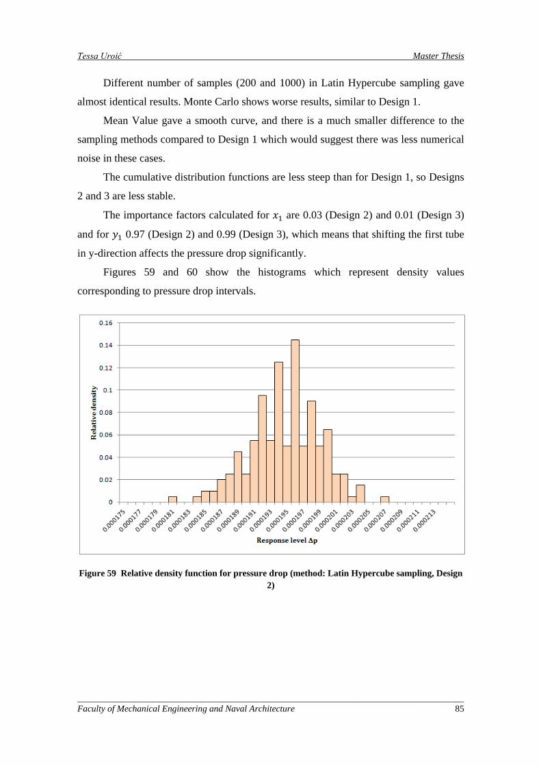
Tessa Uroić Master Thesis
Different number of samples (200 and 1000) in Latin Hypercube sampling gave
almost identical results. Monte Carlo shows worse results, similar to Design 1.
Mean Value gave a smooth curve, and there is a much smaller difference to the
sampling methods compared to Design 1 which would suggest there was less numerical
noise in these cases.
The cumulative distribution functions are less steep than for Design 1, so Designs
2 and 3 are less stable.
The importance factors calculated for 𝑥1 are 0.03 (Design 2) and 0.01 (Design 3)
and for 𝑦1 0.97 (Design 2) and 0.99 (Design 3), which means that shifting the first tube
in y-direction affects the pressure drop significantly.
Figures 59 and 60 show the histograms which represent density values
corresponding to pressure drop intervals.
Figure 59 Relative density function for pressure drop (method: Latin Hypercube sampling, Design 2)
_____________________________________________________________________________________ Faculty of Mechanical Engineering and Naval Architecture 85
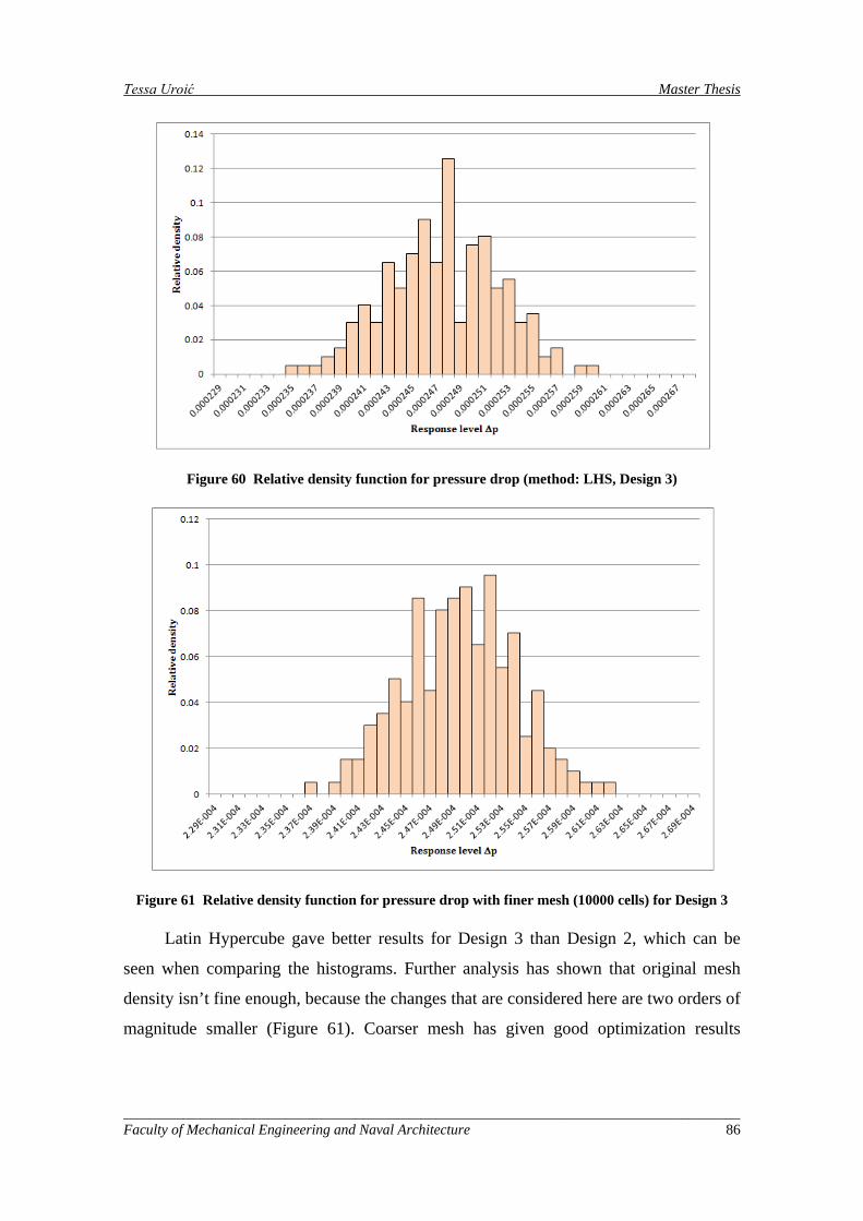
Tessa Uroić Master Thesis
Figure 60 Relative density function for pressure drop (method: LHS, Design 3)
Figure 61 Relative density function for pressure drop with finer mesh (10000 cells) for Design 3
Latin Hypercube gave better results for Design 3 than Design 2, which can be
seen when comparing the histograms. Further analysis has shown that original mesh
density isn’t fine enough, because the changes that are considered here are two orders of
magnitude smaller (Figure 61). Coarser mesh has given good optimization results
_____________________________________________________________________________________ Faculty of Mechanical Engineering and Naval Architecture 86
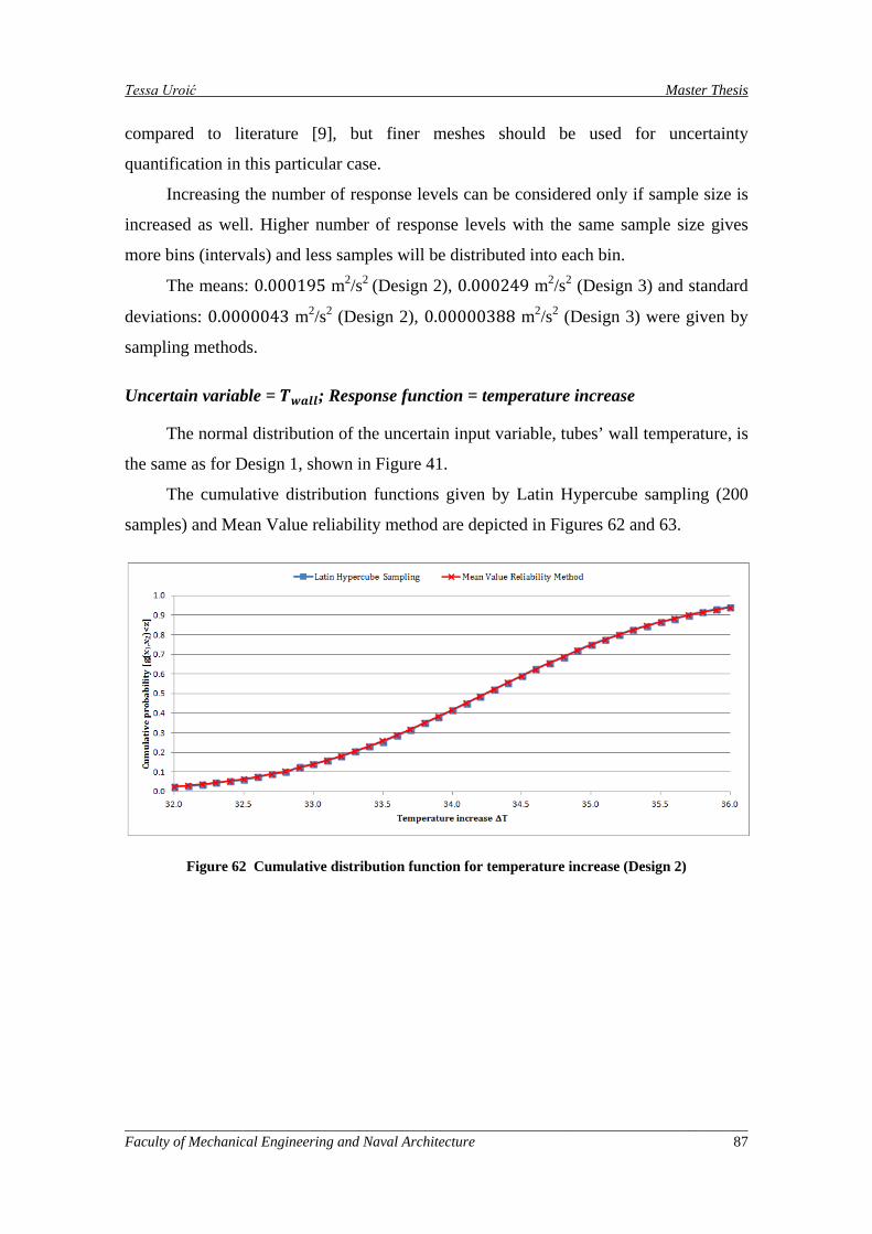
Tessa Uroić Master Thesis
compared to literature [9], but finer meshes should be used for uncertainty
quantification in this particular case.
Increasing the number of response levels can be considered only if sample size is
increased as well. Higher number of response levels with the same sample size gives
more bins (intervals) and less samples will be distributed into each bin.
The means: 0.000195 m2/s2 (Design 2), 0.000249 m2/s2 (Design 3) and standard
deviations: 0.0000043 m2/s2 (Design 2), 0.00000388 m2/s2 (Design 3) were given by
sampling methods.
Uncertain variable = 𝑻𝒘𝒂𝒍𝒍; Response function = temperature increase
The normal distribution of the uncertain input variable, tubes’ wall temperature, is
the same as for Design 1, shown in Figure 41.
The cumulative distribution functions given by Latin Hypercube sampling (200
samples) and Mean Value reliability method are depicted in Figures 62 and 63.
Figure 62 Cumulative distribution function for temperature increase (Design 2)
_____________________________________________________________________________________ Faculty of Mechanical Engineering and Naval Architecture 87
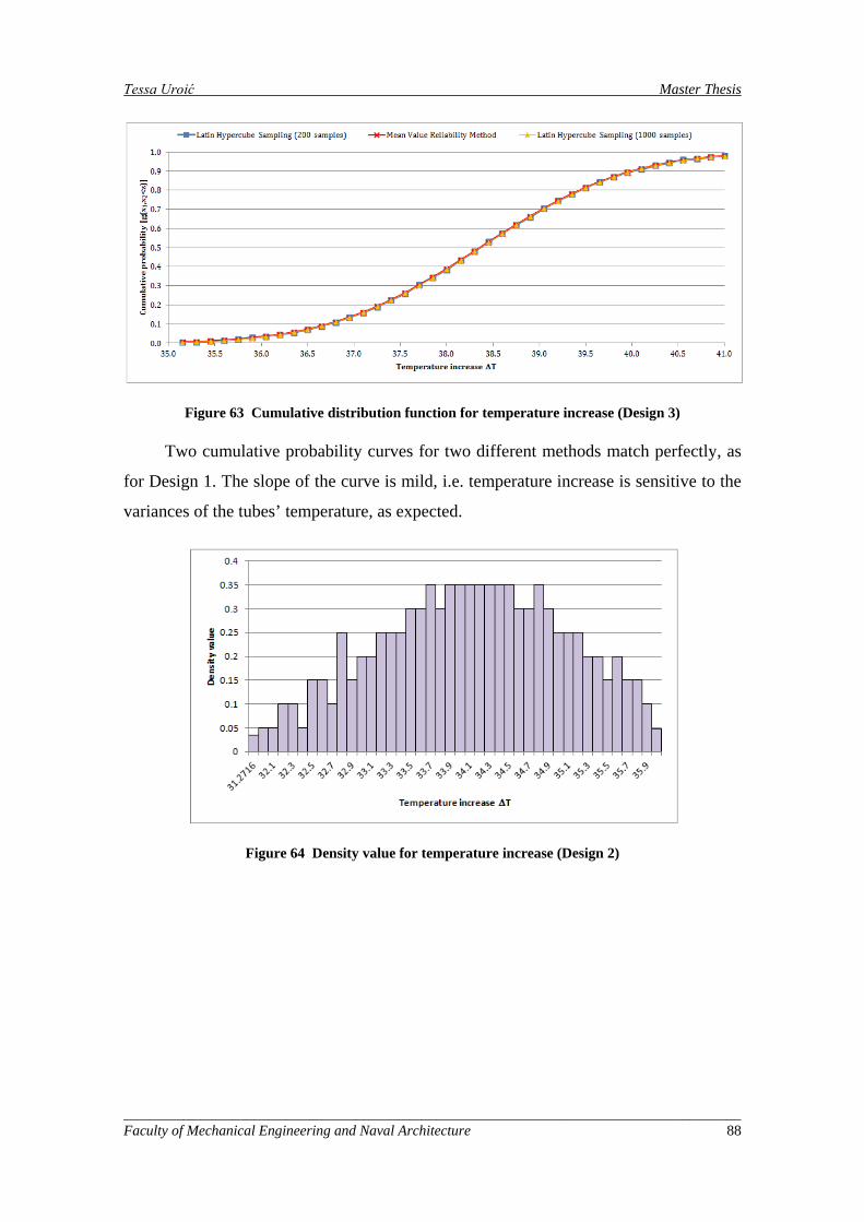
Tessa Uroić Master Thesis
Figure 63 Cumulative distribution function for temperature increase (Design 3)
Two cumulative probability curves for two different methods match perfectly, as
for Design 1. The slope of the curve is mild, i.e. temperature increase is sensitive to the
variances of the tubes’ temperature, as expected.
Figure 64 Density value for temperature increase (Design 2)
_____________________________________________________________________________________ Faculty of Mechanical Engineering and Naval Architecture 88
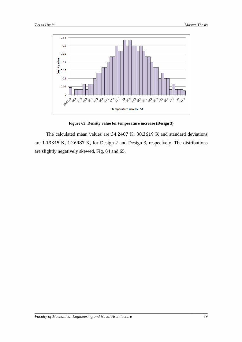
Tessa Uroić Master Thesis
Figure 65 Density value for temperature increase (Design 3)
The calculated mean values are 34.2407 K, 38.3619 K and standard deviations
are 1.13345 K, 1.26987 K, for Design 2 and Design 3, respecively. The distributions
are slightly negatively skewed, Fig. 64 and 65.
_____________________________________________________________________________________ Faculty of Mechanical Engineering and Naval Architecture 89
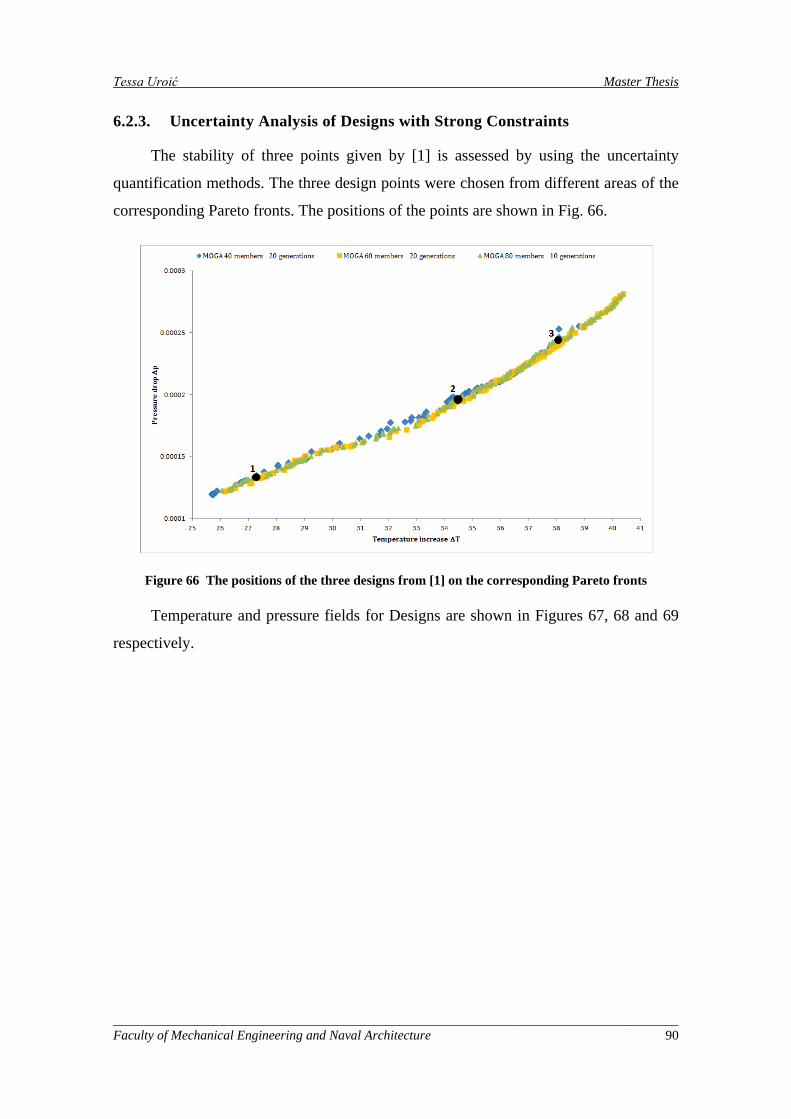
Tessa Uroić Master Thesis
6.2.3. Uncertainty Analysis of Designs with Strong Constraints
The stability of three points given by [1] is assessed by using the uncertainty
quantification methods. The three design points were chosen from different areas of the
corresponding Pareto fronts. The positions of the points are shown in Fig. 66.
Figure 66 The positions of the three designs from [1] on the corresponding Pareto fronts
Temperature and pressure fields for Designs are shown in Figures 67, 68 and 69
respectively.
_____________________________________________________________________________________ Faculty of Mechanical Engineering and Naval Architecture 90
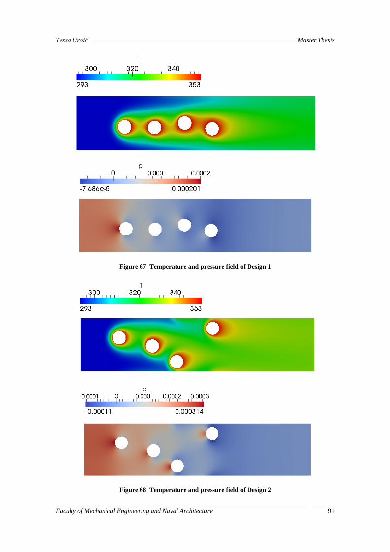
Tessa Uroić Master Thesis
Figure 67 Temperature and pressure field of Design 1
Figure 68 Temperature and pressure field of Design 2
_____________________________________________________________________________________ Faculty of Mechanical Engineering and Naval Architecture 91
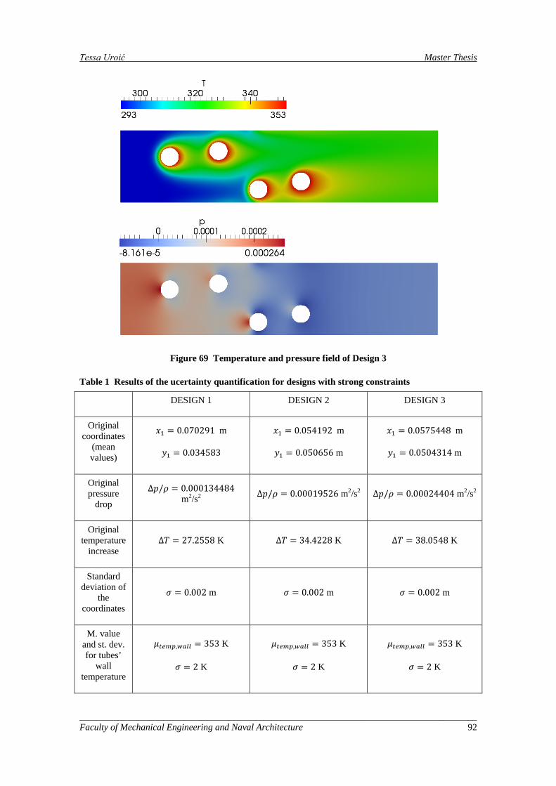
Tessa Uroić Master Thesis
Figure 69 Temperature and pressure field of Design 3
Table 1 Results of the ucertainty quantification for designs with strong constraints
DESIGN 1 DESIGN 2 DESIGN 3
Original coordinates
(mean values)
𝑥1 = 0.070291 m
𝑦1 = 0.034583
𝑥1 = 0.054192 m
𝑦1 = 0.050656 m
𝑥1 = 0.0575448 m
𝑦1 = 0.0504314 m
Original pressure
drop
∆𝑝/𝜌 = 0.000134484 m2/s2 ∆𝑝/𝜌 = 0.00019526 m2/s2 ∆𝑝/𝜌 = 0.00024404 m2/s2
Original temperature
increase ∆𝑇 = 27.2558 K ∆𝑇 = 34.4228 K ∆𝑇 = 38.0548 K
Standard deviation of
the coordinates
𝜎 = 0.002 m 𝜎 = 0.002 m 𝜎 = 0.002 m
M. value and st. dev. for tubes’
wall temperature
𝜇𝑡𝑒𝑚𝑝,𝑤𝑎𝑙𝑙 = 353 K
𝜎 = 2 K
𝜇𝑡𝑒𝑚𝑝,𝑤𝑎𝑙𝑙 = 353 K
𝜎 = 2 K
𝜇𝑡𝑒𝑚𝑝,𝑤𝑎𝑙𝑙 = 353 K
𝜎 = 2 K
_____________________________________________________________________________________ Faculty of Mechanical Engineering and Naval Architecture 92
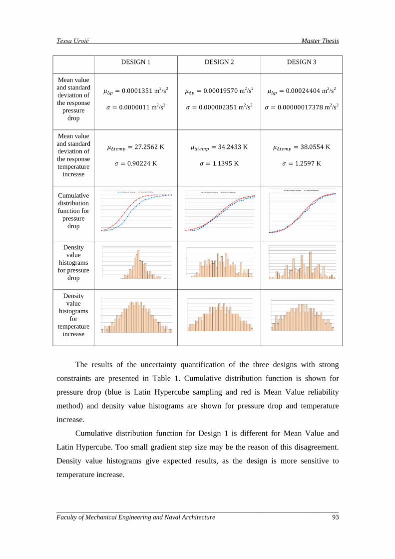
Tessa Uroić Master Thesis
DESIGN 1 DESIGN 2 DESIGN 3
Mean value and standard deviation of the response
pressure drop
𝜇∆𝑝 = 0.0001351 m2/s2
𝜎 = 0.0000011 m2/s2
𝜇∆𝑝 = 0.00019570 m2/s2
𝜎 = 0.000002351 m2/s2
𝜇∆𝑝 = 0.00024404 m2/s2
𝜎 = 0.00000017378 m2/s2
Mean value and standard deviation of the response temperature
increase
𝜇∆𝑡𝑒𝑚𝑝 = 27.2562 K
𝜎 = 0.90224 K
𝜇∆𝑡𝑒𝑚𝑝 = 34.2433 K
𝜎 = 1.1395 K
𝜇∆𝑡𝑒𝑚𝑝 = 38.0554 K
𝜎 = 1.2597 K
Cumulative distribution function for
pressure drop
Density value
histograms for pressure
drop
Density value
histograms for
temperature increase
The results of the uncertainty quantification of the three designs with strong
constraints are presented in Table 1. Cumulative distribution function is shown for
pressure drop (blue is Latin Hypercube sampling and red is Mean Value reliability
method) and density value histograms are shown for pressure drop and temperature
increase.
Cumulative distribution function for Design 1 is different for Mean Value and
Latin Hypercube. Too small gradient step size may be the reason of this disagreement.
Density value histograms give expected results, as the design is more sensitive to
temperature increase.
_____________________________________________________________________________________ Faculty of Mechanical Engineering and Naval Architecture 93

Tessa Uroić Master Thesis
Cumulative distribution functions for both Design 2 and 3 are very similar for
both methods. Density histograms for pressure drops of Designs 2 and 3 didn’t come
out as expected as there is a high dissipation. As it has been shown before, finer
computational mesh may resolve this problem. Density histograms for temperature
increase show sensitivity to tubes’ wall temperature changes. Better distribution of these
histograms could be achieved if wider range of response levels was prescribed, as the
tails of the distribution seem to expand further. Design 1 shows less sensitivity to
temperature changes because it’s initial temperature increase is the smallest (tubes
aligned horizontally).
_____________________________________________________________________________________ Faculty of Mechanical Engineering and Naval Architecture 94
Tessa Uroić Master Thesis
7. Conclusion
Optimization is a discipline of numerical mathematics which aims to improve the
operation of a system or process as good as possible in some defined sense.
Optimization algorithms work to minimize (or maximize) an objective function,
typically calculated by the user simulation code, subject to constraints on design
variables and responses.
Parameters and settings of tube bank heat exchanger multi-objective optimization
were described. The problem consists of finding the best locations of the tubes to
increase heat exchange (i.e. the temperature increase of the fluid) while at the same time
limit the pressure loss. The two corresponding numerical parameters to optimize are the
average temperature difference ∆𝑇 and pressure drop ∆𝑃 between inflow and outflow.
The set of coupled numerical tools to solve the multi-objective optimization
consists of open source optimization software Dakota, open source CFD toolbox
OpenFOAM and open source software for geometry creation Salome. Multi-objective
Genetic Algorithm is used to obtain optimal designs.
Results of the optimization process are presented on corresponding Pareto fronts.
Different parameters of the Multi-objective Genetic Algorithm were examined and
discussed.
It was shown that higher number of evaluations gives more solutions and better
statistical convergence of the Pareto front. Higher mutation rate and crossover rate also
give more possible solutions, as members of the population change more. Designs with
strong and relaxed constraints were also examined and they give similar results.
Uncertainty quantification or nondeterministic analysis is the process of
characterizing input uncertainties, forward propagating these uncertainties through a
computational model, and performing statistical or interval assessments on the resulting
responses. Uncertainty quantification is related to sensitivity analysis in that the
common goal is to gain an understanding of how variations in the parameters affect the
response functions of the engineering design problem. For uncertainty quantification,
some or all of the components of the parameter vector, are considered to be uncertain as
specified by particular probability distributions.
Effect of uncertain tube coordinates and uncertain tubes’ temperature was
examined and presented in graphs and histograms.
_____________________________________________________________________________________ Faculty of Mechanical Engineering and Naval Architecture 95

Tessa Uroić Master Thesis
Depending on the the original positions of the tubes, designs are more or less
stable, i.e. objective functions distributions correspond to uncertain variables'
distributions, however, mesh density effect on the solution should be further examined.
Single-objective optimization wasn't conducted [1], and further development of
the method should be included in future work.
_____________________________________________________________________________________ Faculty of Mechanical Engineering and Naval Architecture 96
Tessa Uroić Master Thesis
References [1] V. Škurić, Master Thesis: Multi-objective Optimization of a Tube Bank Heat
Exchanger, Zagreb, 2014
[2] A. Ravindran, K.M. Ragsdell and G.V. Reklaitis, Engineering optimization: Methods and Applications, United States, 2006
[3] http://en.wikipedia.org/wiki/Uncertainty_quantification
[4] M. Havbro Faber, Statistics and Probability Theory, Springer Science+Business Media, Denmark, 2012
[5] A.M. Hasofer, N.C. Lind, An Exact and Invariant First Order Reliability Format, J. Eng. Mech. Div. Proc ASCE 100 (EMI), 1974
[6] H.O. Madsen, S. Krenk, N.C. Lind, Methods of Structural Safety, New York, United States, 2006
[7] B. Adams, L.Bauman, W. Bohnhoff, K. Dalbey, J. Eddy, M. Ebeida, M. Eldred, P. Hough, K. Hu, J. Jakeman, L. Swiler, and D. Vigil: Dakota: A Multilevel Parallel Object-Oriented Framework for Design Optimization, Parameter Estimation, Uncertainty Quantification, and Sensitivity Analysis, Version 5.4 Reference Manual, Sandia Technical Report SAND2010-2184, United States, 2013
[8] B. Adams, L.Bauman, W. Bohnhoff, K. Dalbey, J. Eddy, M. Ebeida, M. Eldred, P. Hough, K. Hu, J. Jakeman, L. Swiler, and D. Vigil: Dakota: A Multilevel Parallel Object-Oriented Framework for Design Optimization, Parameter Estimation, Uncertainty Quantification, and Sensitivity Analysis, Version 5.4 Theory Manual, Sandia Technical Report SAND2011-9106, United States, 2013
[9] D. Thévenin and G. Janiga, Optimization and Computational Fluid Dynamics, Springer-Verlag Berlin Heidelberg, Berlin, Germany, 2008
[10] C.M. Fonseca, P.J. Fleming, Genetic Algorithms for Multi-objective Optimization: Formulation, Discussion and Generalization, California, United States, 1993
[11] M. Gen, and R. Cheng., Genetic Algorithms & Engineering Optimization, John Wiley & Sons, Inc., NewYork, United States, 2000
[12] L. Wei, Y. Yuying, Multi-objective Optimization of Sheet Metal Forming Process Using Pareto-based Genetic Algorithm, Elsevier, China, 2008
[13] J. Eddy, L. Kemper, Effective Generation of Pareto Sets Using Genetic Programming, University at Buffalo, United States, 2001
[14] J. Wu, and S. Azarm, Metrics for Quality Assessment of a Multiobjective Design Optimization Solution Set, ASME Design Engineering Technical Conferences, 2000
_____________________________________________________________________________________ Faculty of Mechanical Engineering and Naval Architecture 97

Tessa Uroić Master Thesis
[15] D. Barkley, R.D. Henderson, Three-dimensional Floquet Stability Analysis of the Wake of a Circular Cylinder, Journal of Fluid Mechanics, 1996
[16] D. Barkley, Linear Analysis of the Cylinder Wake Mean Flow, Europhysics Letters, 2006
[17] J.H. Ferziger, and M. Perić, Computational Methods for Fluid Dynamics, Springer-Verlag Berlin Heidelberg, Berlin, Germany, 1996
_____________________________________________________________________________________ Faculty of Mechanical Engineering and Naval Architecture 98


![SALOME version 9.4 · 2019-12-18 · The possibility to build and use salome resource manager apart from SALOME has been implemented. 16988 Summary: [CEA] Use of SALOME_Launcherwith](https://img.pdfslide.us/doc/110x75/5fa539dcde7f712e310f98ed/salome-version-94-2019-12-18-the-possibility-to-build-and-use-salome-resource.jpg)