Embed Size (px)
Citation preview
© Florian Moll, 2006; DLR e.V.
Technische Universität München (TUM) Fakultät für Elektrotechnik und Informationstechnik
Master Thesis
Conception and development of an adaptive optics testbed for free-space optical communication
Author: Florian Moll Student ID: 3088025
Supervising institution: German Aerospace Center (DLR) Institute for Measurement Systems and Sensor Technology (TUM) Supervisor: Dipl.-Ing. Markus Knapek (DLR) Dipl.-Ing. Nadine Werth (TUM) Prof. Dr.-Ing. habil. Alexander W. Koch (TUM)
May, 2009
Table of content ii
© Florian Moll, 2006; DLR e.V.
Table of content
TABLE OF CONTENT....................................................................................................................................... II
FIGURES............................................................................................................................................................. IV
TABLES.................................................................................................................................................................X
ACRONYMS ....................................................................................................................................................... XI
SYMBOLS........................................................................................................................................................XIII
ABSTRACT.....................................................................................................................................................XVII
1 INTRODUCTION ....................................................................................................................................... 1
2 OPTICAL TURBULENCE IN THE ATMOSPHERE ............................................................................ 4
2.1 THE ORIGIN OF ATMOSPHERIC TURBULENCE ......................................................................................... 4 2.2 KOLMOGOROV THEORY OF TURBULENCE .............................................................................................. 5
2.2.1 Fluctuations of index-of-refraction ................................................................................................. 5 2.2.2 Atmospheric temporal statistics ...................................................................................................... 9
2.3 DISTORTED WAVE-FRONTS.................................................................................................................. 11
2.3.1 Description of wave-front.............................................................................................................. 11 2.3.2 Origin of wave-front distortions.................................................................................................... 13 2.3.3 Fried parameter and focus spot size ............................................................................................. 13 2.3.4 Representation of wave-fronts with Zernike polynomials ............................................................. 15 2.3.5 G-tilt and Z-tilt: Angle-of-arrival.................................................................................................. 16
2.3.5.1 Definition of the angle-of-arrival......................................................................................................... 16 2.3.5.2 Angle-of-arrival spectral power density for Z-tilt................................................................................ 17 2.3.5.3 Angle-of-arrival spectral power density for G-tilt ............................................................................... 18
2.3.6 Expected aberrations and wave-front tilt ...................................................................................... 20 2.4 SCINTILLATION EFFECTS ..................................................................................................................... 21
3 ADAPTIVE OPTICS IN FREE SPACE OPTICAL COMMUNICATIONS....................................... 24
3.1 PRINCIPLE OF ADAPTIVE OPTICS SYSTEMS ........................................................................................... 24 3.2 WAVE-FRONT CORRECTION OF THE COMMUNICATION SIGNAL ............................................................ 25 3.3 REQUIREMENTS ON THE ADAPTIVE OPTICS SYSTEM............................................................................. 28
3.3.1 Spatial requirements ..................................................................................................................... 28 3.3.2 Temporal requirements ................................................................................................................. 30
4 CONCEPT AND DESIGN OF THE TESTBED .................................................................................... 31
Table of content iii
© Florian Moll, 2006; DLR e.V.
4.1 THEORY AND APPLICABILITY OF AN OPTICAL TURBULENCE GENERATOR ............................................ 31 4.2 CONCEPT OF THE TESTBED .................................................................................................................. 34 4.3 OPTICAL TURBULENCE GENERATOR .................................................................................................... 37
4.3.1 State of the art of optical turbulence generators........................................................................... 37 4.3.2 Hot-air optical turbulence generator ............................................................................................ 38
4.4 FOCUS CAMERA................................................................................................................................... 43
4.4.1 Setup.............................................................................................................................................. 43 4.4.2 Principle of angle-of-arrival measurement ................................................................................... 45 4.4.3 Determination of atmosphere statistics with the focus camera ..................................................... 45
4.5 SHACK HARTMANN WAVE-FRONT SENSOR.......................................................................................... 46 4.6 DEFORMABLE MIRROR ........................................................................................................................ 48 4.7 OPTICAL LAYOUT................................................................................................................................ 52
4.7.1 Laboratory setup ........................................................................................................................... 52 4.7.2 Achromatic design of the transmitter ............................................................................................ 53 4.7.3 Achromatic design of the receiver................................................................................................. 54 4.7.4 Chromatic design of the receiver .................................................................................................. 55
4.8 FURTHER COMPONENTS....................................................................................................................... 58
5 MEASUREMENTS AND ANALYSIS OF THE ARTIFICIAL TURBULENCE............................... 60
5.1 MEASUREMENT ARRANGEMENT.......................................................................................................... 60 5.2 MEASUREMENT OF ANGLE-OF-ARRIVAL TIME SERIES.......................................................................... 61 5.3 POWER SPECTRAL DENSITY OF ANGLE-OF-ARRIVAL ............................................................................ 65 5.4 CALIBRATION OF HOT AIR TURBULENCE GENERATOR WITH MEASUREMENTS OF FRIED
PARAMETER AND TURBULENCE STRENGTH.......................................................................................... 68
6 CONCLUSION.......................................................................................................................................... 71
REFERENCES.................................................................................................................................................... 73
APPENDIX.......................................................................................................................................................... 77
A WIND SPEED............................................................................................................................................ 77
B MOUNTING DISTANCES OF TESTBED OPTICS............................................................................. 78
C ZERNIKE MODES................................................................................................................................... 80
Figures iv
© Florian Moll, 2006; DLR e.V.
Figures
Figure 1-1: Illustration of a down-link from the Earth observation satellite TerraSAR-X
to an optical ground station at DLR Oberpfaffenhofen. ................................................. 2
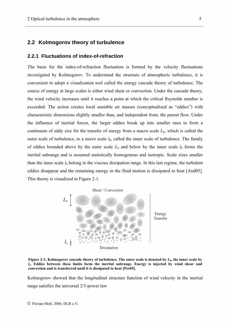
Figure 2-1: Kolmogorov cascade theory of turbulence. The outer scale is denoted by L0,
the inner scale by lo. Eddies between these limits form the inertial subrange.
Energy is injected by wind shear and convection and is transferred until it is
dissipated to heat [Per05]. .............................................................................................. 5
Figure 2-2: Modified Hufnagel-Valley profile for night- and daytime conditions for a
ground station at 600 m above sea level. The input values are 21 m/s for the wind
speed and a near ground Cn2 of 1.7*10-14 m-2/3 for night time and 1.7*10-13 m-2/3
for daytime...................................................................................................................... 8
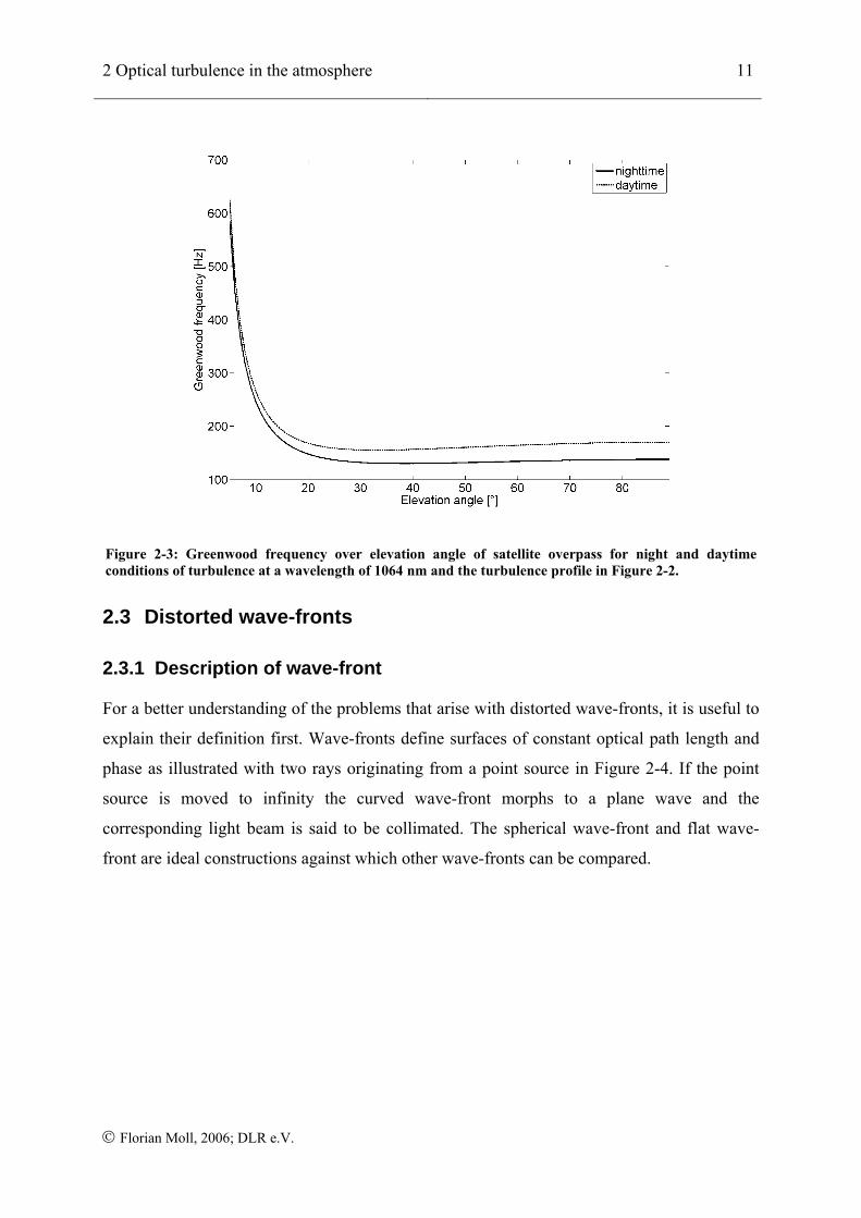
Figure 2-3: Greenwood frequency over elevation angle of satellite overpass for night and
daytime conditions of turbulence at a wavelength of 1064 nm and the turbulence
profile in Figure 2-2...................................................................................................... 11
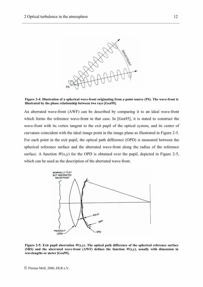
Figure 2-4: Illustration of a spherical wave-front originating from a point source (PS).
The wave-front is illustrated by the phase relationship between two rays [Gea95]..... 12
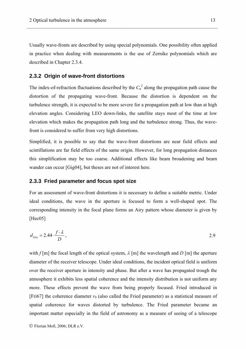
Figure 2-5: Exit pupil aberration W(x,y). The optical path difference of the spherical
reference surface (SRS) and the aberrated wave-front (AWF) defines the function
W(x,y), usually with dimension in wavelengths or meter [Gea95]. ............................. 12
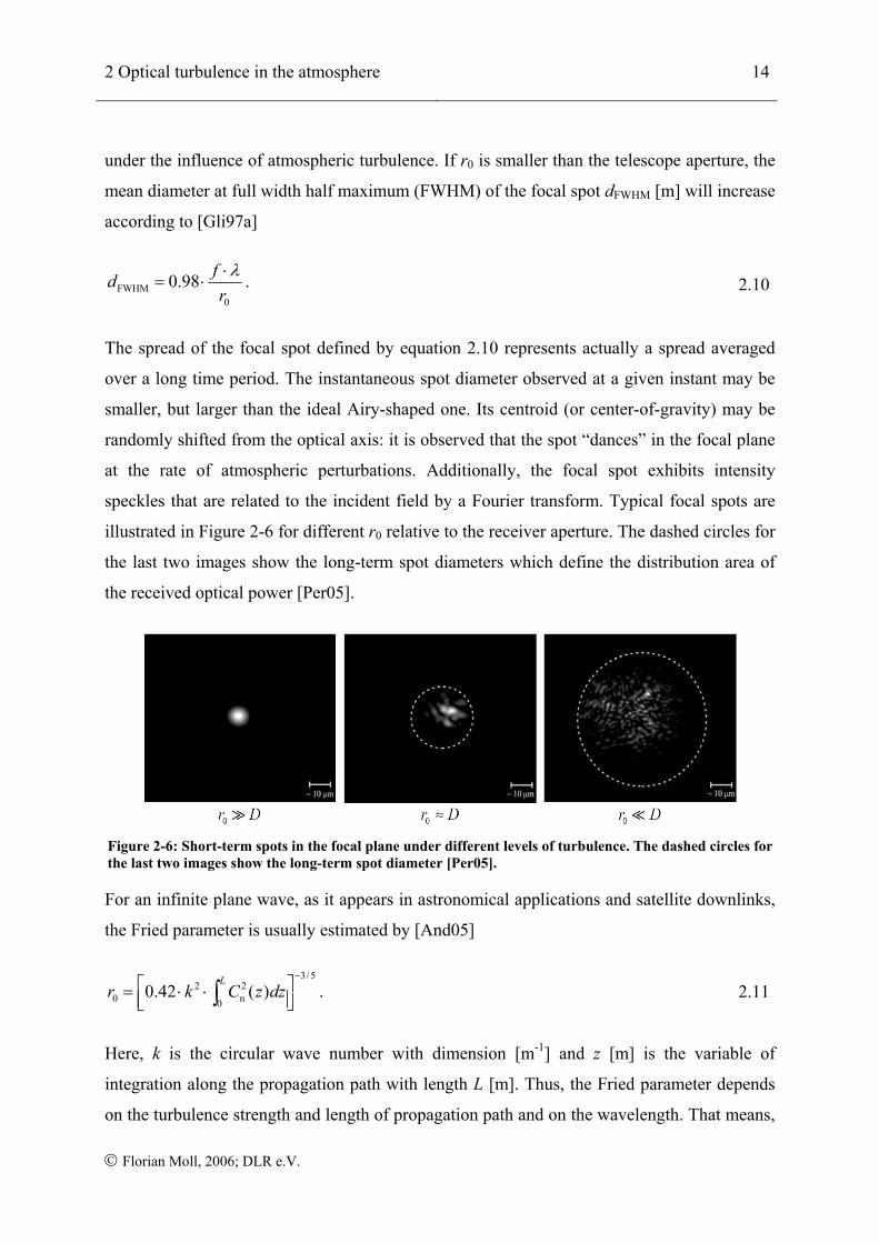
Figure 2-6: Short-term spots in the focal plane under different levels of turbulence. The
dashed circles for the last two images show the long-term spot diameter [Per05]....... 14
Figure 2-7: Power spectral densities for G- and Z-tilts (blue and black line) for two wind
speeds. The receiver aperture is 40 cm, the propagation path is 1 km with a Cn2 of
1*10-13 m2/3. .................................................................................................................. 20
Figure 2-8: Tip-tilt and wave-front standard deviation for λ = 1064 nm and two aperture
sizes. The standard deviation of tip-tilt corrected wave-front is wavelength
dependent. However, the standard deviation of angle-of-arrival is not.
Figures v
© Florian Moll, 2006; DLR e.V.
Considering a real LEO satellite down-link scenario, r0 is expected to vary
between 10 mm and 200 mm for different elevation angles, respectively. .................. 21
Figure 2-9: Probability distribution of the received intensity (point receiver) for several
elevation angles. These data have been measured during the KIODO experiment
which consisted in an optical downlink from a Japanese LEO satellite, λ = 847
nm. The intensity was measured by camera in digital numbers (DN) [Per07]. ........... 22
Figure 2-10: Measured intensity field in the pupil plane of a 40-cm telescope.
Scintillation speckled can be observed [Hor07]. .......................................................... 22
Figure 3-1: The main elements of an adaptive optics system. The wave-front sensor
measures the aberrations and sends the information to the deformable mirror to
flatten the wave-front. A camera, or respectively a fiber, in the corrected focus
takes the corrected image [Gli97a]. .............................................................................. 25
Figure 3-2: The main optical elements of the optical system of ALFA: The tip-tilt mirror
(TM) corrects the image motion. The first focusing mirror (FM 1) images the
telescope pupil onto the deformable mirror (DM). After the DM, the telescope
focus is reimaged by the second focus mirror (FM 2). The beam-splitter (BS)
reflects a beam to the science camera and transmits a beam to the wave-front
sensor arm [Gli97a]. ..................................................................................................... 25
Figure 3-3: Strehl ratio and wave-front variance over D/r0 for different numbers of
corrected Zernike modes based on the results of [Nol76]. The run of N = 3
corresponds to the correction of piston, tip and tilt, N = 6 adds removal of
defocus and astigmatism............................................................................................... 28
Figure 4-1: Concept of the adaptive optics testbed. The blue elements denote the main
optical path. The first four ones comprise the source, the last seven ones the
receiver. The orange elements are to characterize and calibrate the artificial
turbulence. The green ones contain elements for system tests and measurements
behind the wave-front correction.................................................................................. 36
Figure 4-2: Concept of hot-air turbulence generator. The air is forced into the mixing
chamber through inputs 1 and 2. A heating element warms up one of the flows
and air straigtheners produce two laminar flows that collide in the mixing
Figures vi
© Florian Moll, 2006; DLR e.V.
chamber. The mixed air leaves the box at the two outflows. The laser beam
passes the turbulence through the wholes at 6 and 7. ................................................... 39
Figure 4-3: Result of the component research. Left above, the air fan from Ebm Papst,
left under the 2.3 kw electrical heating element from Friedrich Würth
Produktions GmbH, and the honey-comb filter from Plascore. ................................... 40
Figure 4-4: Test version of hot-air optical turbulence generator (above). The two
thermometers on top measure the temperature of the air flows. This version
shows an amendment to the initial design on the side of the hot-air intake. This is
the small additional box on the right that was necessary to enlarge the distance
between the fan and heater which is shown in the picture in the middle. Here also
the action of the heater is clearly visible. Below, the OTG is imaged without its
top which reveals position of the air straighteners. ...................................................... 42
Figure 4-5: Design study of hot-air OTG version 2. As basis version 1 is used slightly
modified, which means that, in Figure 4-2, hole number 7 is enlaged and hole
number 6 is filled. An extension is placed next to the mixing chamber which
makes the turbulent flow propagate towards hole 7. The laser beams are shot
transversal through the holes in the extension.............................................................. 43
Figure 4-6: Setup of the focus camera. Left below in the Mikrobank assembly is the
aperture lens of the telescope system (1). The light beam enters from the left. The
pellicle beam splitter (2) guides the beam towards the camera. The focusing lens
(3) creates the focus spot on the CCD of the camera (5). An additional optical
attenuation element (4) prevents the CCD from saturation. ......................................... 44
Figure 4-7: Concept of angle-of-arrival measurement with the focus camera. The
displacement of the focus spot relative to a reference position on the CCD is
measured. With knowledge of the effective focal length of the optical system
(here represented by a single lens) the angle-of-arrival can be calculated. .................. 45
Figure 4-8: Measurement principle of a Shack-Hartmann sensor. The incoming wave-
front is sub-divided by the lenslet array and the image centroid in every sub-
image is shifted according to the average wave-front slope over the sub-aperture
formed by the lenslet [Gli97a]...................................................................................... 47
Figures vii
© Florian Moll, 2006; DLR e.V.
Figure 4-9: Setup of the Shack-Hartmann wave-front sensor in the testbed. The lenslet
array (2) is mounted in the optical path in a way that it can be rotated by using a
screw for adjustment with the camera (3). ................................................................... 47
Figure 4-10: Mean residual wave-front error averaged over 100 phase screens obeying
Kolmogorov statistics with strength of D/r0 = 9, piston and tip-tilt removed
[Dev08]. The BMC140 performs best in this measurement......................................... 49
Figure 4-11: Strehl ratio after fitting the five mirrors to a sample of 100 atmospheric
wave-fronts with D/r0 = 9 [Far07]. Here, the BMC140 needs many modes to be
corrected. ...................................................................................................................... 50
Figure 4-12: BMC140 deformable mirror (1), integrated in the testbed. On the left are
the driver electronics (2) which are wired to the DM by four flat ribbon cables. ........ 51
Figure 4-13: Testbed setup in optics laboratory of the OCG. The transmitter on the
optical table under the clean room unit (3) sends the light beam through the OTG
(2). The beam is reflected with the flat mirror (1), propagates through the OTG a
second time and hits the receiver on the optical table (3). ........................................... 52
Figure 4-14: Setup of testbed transmitter part. The aperture of the Newton telescope (1)
bears a cover to supply an obscuration-free collimated beam. One of both laser
diodes (2,3), driven by a laboratory power supply (4), serve as input to the
telescope. ...................................................................................................................... 53
Figure 4-15: Collimation test of source telescope (Newton type) with shear plate from
Melles Griot. The left picture shows how the black line runs in parallel to the
interference fringes which proofs collimation of the beam. The left picture shows
the Newtonian telescope. The black Thorlabs tubus on top is height adjustable to
put the fiber in focus. .................................................................................................... 54
Figure 4-16: Illustration of a Zemax ray trace of a 4:1 beam compressor build by two
off-axis concave mirrors (left). Simulated elements are taken from the Edmund
Optics catalogue. The simulation shows a pupil image in case of a spider in the
aperture. The pupil image is only partially sharp. ........................................................ 55
Figures viii
© Florian Moll, 2006; DLR e.V.
Figure 4-17: Optical layout of adaptive optics testbed receiver part. The layout is
designed with Zemax. The rays enter the system at the aperture stop and
thereafter are directed to the respective sensors. .......................................................... 56
Figure 4-18: Adaptive optics testbed receiver part assembled on the optical table. The
beam enters the system trough the aperture lens and stop (1). The picture misses
the deformable mirror which is located to the left of imaging lens 6. The FPA
sensor and the DIMM are not assembled. .................................................................... 58
Figure 5-1: Dependency of temperature difference from dimmer scale for the hot-air
OTG at Vfan = 10 V. ...................................................................................................... 61
Figure 5-2: Image series for increasing temperature difference and Vfan = 10 V as
captured by the focus camera. With increasing Tdiff, the speckle pattern of the
spot becomes more distinct........................................................................................... 62
Figure 5-3: Time series of AoA for increasing temperature difference and Vfan = 10 V,
whereas Tdiff increases from left to right and up to down............................................. 63
Figure 5-4: Time series of AoA for temperature difference of 133 K and Vfan = 10 V for
the x- and y-axis. Both directions appear to have same order of magnitude of
AoA stroke.................................................................................................................... 64
Figure 5-5: Time series of AoA for temperature difference of 133 K and Vfan = 10 V for
the x- and y-axis. Only a short measurement interval is plotted to highlight the
strong peaks in the time series that cause severe disturbances which happen in x-
and y-direction. ............................................................................................................. 64
Figure 5-6: Autocorrelation function of AoA measurement at Tdiff = 116°C and fan at
10 V. A correlation time can be measured as the full width half maximum of this
ACF. ............................................................................................................................. 65
Figure 5-7: Autocorrelation function of AoA measurement at Tdiff = 116°C and fan at
10 V, zoomed from -0.5 to 0.5 τ to highlight the periodic disturbances. ..................... 66
Figure 5-8: PSD with V = 10 V, DS=1.0, 1064nm. ................................................................. 67
Figure 5-9: PSD of back-to-back measurements...................................................................... 67
Figure 5-10: Measurement of r0 for a fan speed at V = 10 V and dimmer scale = max.......... 68
Figures ix
© Florian Moll, 2006; DLR e.V.
Figure 5-11: Measurement of r0 over dimmer scale with fan speed at V = 10 V.................... 69
Figure 5-12: Measurement of Cn2 over dimmer scale with fan speed at V = 10 V. ............... 70
Figure 6-1: Illustration of the Bufton wind model for vg = 5 m/s (dashed line). The
viewing angle at ground station height of 600 m amounts 90° elevation (zenith
view). The grey line shows the additional pseudo wind speed due to plain satellite
motion at an orbit of 510 km height and zenith over flight (the resulting slew rate
is 15 mrad/s). The sum of both results in the effective transversal wind speed
(solid line)..................................................................................................................... 78
Tables x
© Florian Moll, 2006; DLR e.V.
Tables
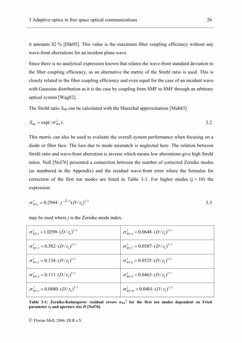
Table 3-1: Zernike-Kolmogorov residual errors σWF2 for the first ten modes dependent on
Fried parameter r0 and aperture size D [Nol76]. .......................................................... 26
Table 4-1: Comparison of influence of AoA fluctuation on the spot movement in the
image plane for same focus lenses. Because the significant ratios D/r0 and D/feff
are the same, the resulting spot movement due to AoA fluctuations is the same
(last line). ...................................................................................................................... 33
Table 4-2: Specifications of the BMC140 that is chosen to be implemented in the
testbed. .......................................................................................................................... 51
Acronyms xi
© Florian Moll, 2006; DLR e.V.
Acronyms
AO Adaptive Optics
AoA Angle-of-Arrival
ACF AutoCorrelation Function
ALFA Adaptive optics with a Laser For Astronomy
AR Anti-Reflection
AWF Aberrated Wave-Front
BS Beam Splitter
CCD Charge-Coupled Device
DLR Deutsches Zentrum für Luft- und Raumfahrt (German Aerospace Center)
DM Deformable Mirror
DN Digital Number
DS Dimmer Scale of the power dimmer
ESO European Southern Observatory
FM Focusing Mirror
FPA Fine Pointing Assembly
FSO Free Space Optics
FWHM Full width half maximum
GEO Geostationary Earth Orbit
G-tilt Center-of-gravity tilt
HAP High Altitude Platform
IFC Imaging Foundation Classes
IR Infra-Red
KIODO KIrari Optical Downlink to Oberpfaffenhofen
LEO Low Earth Orbit
Acronyms xii
© Florian Moll, 2006; DLR e.V.
MAPS Multi Atmospheric Phase screens and Stars
OCG Optical Communications Group
OGS Optical Ground Station
OPD Optical Path Difference
OTG Optical Turbulence Generator
PDF Probability Density Function
PEEK Polyetheretherketon
POM Polyoxymethylen
PSD Power Spectral Density
PTFE Polytetrafluorethylen
RMS Root-Mean-Squared
SHWFS Shack-Hartmann Wave-front Sensor
SMF Single-Mode Fiber
SLM Spatial Light Modulator
SRS Spherical Reference Surface
TM Tip-tilt mirror
UAV Unmanned Aeronautical Vehicle
VOA Variable Optical Attenuator
WFS Wave-Front Sensor
Z-tilt Zernike tilt
4QD 4-Quadrant-Detector
Symbols xiii
© Florian Moll, 2006; DLR e.V.
Symbols
aj Coefficient of Zernike mode expansion [waves]
D Distance [m]
dAiry Diameter of Airy focal spot [m]
dFWHM FWHM diameter of focal spot [m]
f Focal length [m]
fBW Bandwidth of adaptive optics control loop [Hz]
feff Effective focal length [m]
fG Greenwood frequency [Hz]
fk Knee frequency of angle-of-arrival power spectral density [Hz]
fTG Fundamental tracking frequency of G-tilt [Hz]
h Height above sea level [m]
j Zernike mode numbering index [-]
k Circular wave number [m-1]
l Radial degree of Zernike polynomial [-]
l0 Inner scale of turbulence [m]
m Azimuthal frequency of Zernike polynomial [-]
n Index-of-refraction [-]
p Variable [-]
q Variable [-]
r Polar coordinate radial direction [m]
r Coordinate vector [m]
rc Actuator spacing of the deformable mirror [m]
r0 Fried parameter [m]
Symbols xiv
© Florian Moll, 2006; DLR e.V.
u Cartesian coordinate u-direction in the aperture plane [m]
v Cartesian coordinate v-direction in the aperture plane [m]
vg Wind speed at the ground [m/s]
vn Normalized wind velocity component [s-1]
vrms Square root of the RMS of the wind between 5 km and 20 km height [m/s]
v(z) Propagation path distance dependent wind speed [m/s]
x Cartesian coordinate x-direction in the focal plane [m]
xSpot One axis spot movement [m]
y Cartesian coordinate y-direction in the focal plane [m]
z Propagation path distance [m]
A parameter for ground near values of Hufnagel-Valley model [m-2/3]
Ai(r) Normalized incident optical field [-]
Am(r) Normalized mode profile in the receiver aperture plane [-]
Cn2 Index-of-refraction structure constant [m-2/3]
CT2 Temperature structure constant [K2/m2/3]
CV2 Longitudinal wind structure constant [m4/3/s2]
D Aperture diameter [m]
Dn(R) Index-of-refraction structure function [-]
DRR(R) Longitudinal structure function of wind velocity [m2/s2]
DT(R) Temperature structure function [K2]
DTM Diameter of tip-tilt mirror [m]
HGS Height of ground station above sea level [m]
I(x,y) Image intensity [-]
Ji(j) Bessel function of i-th kind [-]
Symbols xv
© Florian Moll, 2006; DLR e.V.
L Length of propagation path [m]
L0 Outer scale of turbulence [m]
Mtilt Maximum atmospheric tilt [rad]
MT Transversal magnification [-]
Mx Centroid of image intensity in x-direction [m]
N Number of corrected Zernike modes [-]
NNA Numerical aperture [-]
P Pressure [mb]
Pa Power in the receiver aperture plane [W]
Pc Power coupled in fiber [W]
R Separation distance [m]
SDM Stroke of deformable mirror [rad]
SSR Strehl ratio [-]
STM Stroke of tip-tilt mirror [rad]
T Temperature [K]
Tdiff Temperature difference of the hot-air OTG [K]
V Velocity component [m/s]
Vfan Fan voltage [V]
W(x,y) Wave-front function [waves]
Zeven j Zernike mode, notation with one index [-]
αAoA Angle-of-arrival [rad]
γ Polar coordinate azimuthal direction [°]
ηc Fiber coupling efficiency [-]
κ Constant of deformable mirror [-]
λ Wavelength of electro-magnetic wave [m]
Symbols xvi
© Florian Moll, 2006; DLR e.V.
ψ Zenith angle [°]
σtemp2 Temporal residual wave-front variance [rad2]
σtilt Standard deviation of wave-front tilt [rad]
σWF Tilt corrected standard deviation of wave-front [rad]
τ Time difference of ACF [s]
φ(x,y) Wave-front function [rad]
ωs Slew rate of satellite [rad/s]
Θ Acceptance angle of optical system [°]
Σ0 Wave-front coherence outer scale [m]
ΦG(f) One axis angle-of-arrival power spectral density of G-tilt [rad2/Hz]
ΦZ(f) One axis angle-of-arrival power spectral density of Z-tilt [rad2/Hz]
Abstract xvii
© Florian Moll, 2006; DLR e.V.
Abstract
Optical free space communications are an efficient approach to transmit high data-rates with
small antennas and low power consumption over large distances. Possible scenarios are links
between satellites, up- and down-links from and to ground stations as well as all kinds of links
between aeronautical vehicles. The links that involve propagation of the electro-magnetic
wave through the atmosphere are critical. Here, signal quality may be degraded severely due
to wave-front distortions. With the exploitation of adaptive optics these wave-front distortions
can be compensated and system performance enhanced. In the framework of this thesis, a
laboratory testbed is built up which offers the scientist a comfortable support for the
development and test of techniques related to adaptive optics and free-space optical
communication. The core components are a hot-air optical turbulence generator, a deformable
mirror, and a Shack-Hartmann wave-front sensor. The emphasis of this thesis lies on the
development and test of the turbulence generator, the overall concept of the testbed, and its
optical design. The testbed makes is possible to reproduce test scenarios with realistic ratios
of aperture size over Fried parameter.
1 Introduction 1
© Florian Moll, 2006; DLR e.V.
1 Introduction
The increasing need for high communication bandwidths all over the world pushes research
and development to search new communication techniques and schemes that are most suitable
for the particular areas of application.
Optical free space communications, often simply called free space optics (FSO), happened to
be explored and further developed for the last four decades especially to fulfill the needs of
aeronautical and space applications. FSO is all about the transmission of modulated electro-
magnetic waves in the visible and infrared spectrum through the atmosphere. Because the
propagation path changes in space and time, its random behavior must be of major concern of
ongoing research. Atmospheric effects like rain, clouds and temperature fluctuations influence
light propagation and may degrade the quality of transmitted signals severely.
Similar to transmission with optical fibers, free space optics can offer high data rates but also
the same flexibility as wireless microwave systems. The short wavelengths allow a more
compact design of components and lower power consumption than microwave systems do,
which is very important for aeronautical and space systems. Furthermore, it is resistant of
spying due to the very small convergence angle of the beam. All this presents free space
optical communications to be an attractive alternative for many kinds of wireless
communication scenarios. Future applications may include networks of HAPS (high altitude
platforms, hovering in the stratosphere), UAVs (unmanned aerial vehicles) and airplanes,
whereas all this aeronautical objects can be optically connected amongst each other and/or
additional satellites. By now, there happen to be several optical communication terminals in
orbit, either mounted on a GEO satellite, like ARTEMIS, or LEO satellites, like SPOT4,
OICETS, NFIRE and TerraSAR-X [Sod07]. Especially the last one is of great interest since,
as an Earth observation satellite, it hosts a terminal capable of doing inter-satellite-links
(ISLs) at 5.6 Gbit/s, which were successfully demonstrated, and down-links to Earth, which
are in test phase at the moment, (Figure 1-1). The communication scheme here comprises
coherent reception and thus has high demands on temporal and spatial coherence of the laser
light. And here lies the connection between the focus of this thesis and practical application in
communications. The use of adaptive optics (AO) has proven to be feasible in boosting
telescope performance in astronomy. Now, this technique shall be applied to Earth bound
1 Introduction 2
© Florian Moll, 2006; DLR e.V.
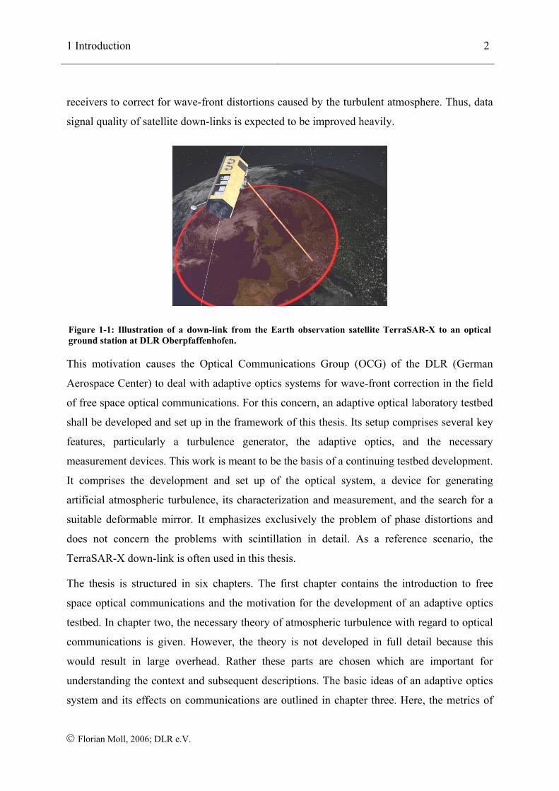
receivers to correct for wave-front distortions caused by the turbulent atmosphere. Thus, data
signal quality of satellite down-links is expected to be improved heavily.
Figure 1-1: Illustration of a down-link from the Earth observation satellite TerraSAR-X to an optical ground station at DLR Oberpfaffenhofen.
This motivation causes the Optical Communications Group (OCG) of the DLR (German
Aerospace Center) to deal with adaptive optics systems for wave-front correction in the field
of free space optical communications. For this concern, an adaptive optical laboratory testbed
shall be developed and set up in the framework of this thesis. Its setup comprises several key
features, particularly a turbulence generator, the adaptive optics, and the necessary
measurement devices. This work is meant to be the basis of a continuing testbed development.
It comprises the development and set up of the optical system, a device for generating
artificial atmospheric turbulence, its characterization and measurement, and the search for a
suitable deformable mirror. It emphasizes exclusively the problem of phase distortions and
does not concern the problems with scintillation in detail. As a reference scenario, the
TerraSAR-X down-link is often used in this thesis.
The thesis is structured in six chapters. The first chapter contains the introduction to free
space optical communications and the motivation for the development of an adaptive optics
testbed. In chapter two, the necessary theory of atmospheric turbulence with regard to optical
communications is given. However, the theory is not developed in full detail because this
would result in large overhead. Rather these parts are chosen which are important for
understanding the context and subsequent descriptions. The basic ideas of an adaptive optics
system and its effects on communications are outlined in chapter three. Here, the metrics of
1 Introduction 3
© Florian Moll, 2006; DLR e.V.
fiber coupling efficiency and Strehl ratio are used to evaluate the effect of AO systems. The
fourth chapter comprises the main part of the work, the testbed development and setup. Here,
a description of the concept of the testbed with all its key features is given. The optical design,
the turbulence generator, the focus camera for measuring the turbulence, the choice of the
deformable mirror and the all over setup are explained in detail. Furthermore, a sub-chapter is
dedicated to the Shack-Hartmann sensor, where some contributions to its development could
be given in the framework of the testbed development. Chapter five presents the
measurements of the focus camera together with its analysis. Finally, in chapter six, a
discussion is done to clear out achieved and missed goals and suggestions of future work. In
the appendix, some more detailed explanations are given, which are not necessary to follow
and understand the thesis, but may be interesting for the reader.
2 Optical turbulence in the atmosphere 4
© Florian Moll, 2006; DLR e.V.
2 Optical turbulence in the atmosphere
2.1 The origin of atmospheric turbulence
Classical studies of turbulence were concerned with fluctuations in the velocity field of a
viscous fluid. In particular, it was observed that the longitudinal wind velocity associated with
the turbulent atmosphere fluctuates randomly about its mean value. That is, the wind velocity
field assumes the nature of a random field, which means that at each point in space and time
within the flow the velocity may be represented by a random variable. Turbulent motion of
the atmosphere in the presence of moisture and temperature gradients gives rise to
disturbances in the atmosphere’s refractive index in the form of cells called optical turbules.
Early studies of Kolmogorov suggest that a subclass of all optical turbules has a degree of
statistical consistency that permits a meaningful theoretical treatment [And05]. Kolmogorov
published in his paper “The local structure of turbulence in incompressible viscous fluid for
very large Reynolds numbers” in 1941, which later was translated into English [Kol91], that
in this domain it is possible to assume statistical homogeneity and isotropy when the
Reynolds number of the flow is sufficiently large. This is very useful for the use of models
that describe the turbulent behavior. This paper also contains Kolmogorov’s famous “two-
third power law” that postulates a particular behavior of the velocity structure function over
separation of measurement points. Thus, most research in the field of optical turbulence in the
atmosphere is related to the Kolmogorov theory of turbulence. By the way, his “two-third
power law” is probably responsible for the quite frequent “odd” power laws in analytic
expressions dealing with atmospheric turbulence.
The present chapter deals with an introduction into what is atmospheric turbulence, its effects
on wave propagation and how these can be measured. The basic principles are shown and
some of the analytical expressions are evaluated to give a better insight. The focus is always
on phase distortion since these can be corrected with adaptive optics systems. However, a
brief description of scintillation effects is also given at the end of the chapter because these
may cause problems in wave-front sensing.
2 Optical turbulence in the atmosphere 5
© Florian Moll, 2006; DLR e.V.
2.2 Kolmogorov theory of turbulence
2.2.1 Fluctuations of index-of-refraction
The basis for the index-of-refraction fluctuation is formed by the velocity fluctuations
investigated by Kolmogorov. To understand the structure of atmospheric turbulence, it is
convenient to adopt a visualization tool called the energy cascade theory of turbulence. The
source of energy at large scales is either wind shear or convection. Under the cascade theory,
the wind velocity increases until it reaches a point at which the critical Reynolds number is
exceeded. The action creates local unstable air masses (conceptualized as “eddies”) with
characteristic dimensions slightly smaller than, and independent from, the parent flow. Under
the influence of inertial forces, the larger eddies break up into smaller ones to form a
continuum of eddy size for the transfer of energy from a macro scale L0, which is called the
outer scale of turbulence, to a micro scale l0, called the inner scale of turbulence. The family
of eddies bounded above by the outer scale L0 and below by the inner scale l0 forms the
inertial subrange and is assumed statistically homogenous and isotropic. Scale sizes smaller
than the inner scale l0 belong to the viscous dissipation range. In this last regime, the turbulent
eddies disappear and the remaining energy in the fluid motion is dissipated to heat [And05].
This theory is visualized in Figure 2-1.
Figure 2-1: Kolmogorov cascade theory of turbulence. The outer scale is denoted by L0, the inner scale by lo. Eddies between these limits form the inertial subrange. Energy is injected by wind shear and convection and is transferred until it is dissipated to heat [Per05].
Kolmogorov showed that the longitudinal structure function of wind velocity in the inertial
range satisfies the universal 2/3-power law
2 Optical turbulence in the atmosphere 6
© Florian Moll, 2006; DLR e.V.
( )2 2 2 3RR 1 2 V( )D R V V C R= − = , 2.1
where V1 [m/s] and V2 [m/s] represent velocity components at two points separated by the
distance R [m]. The factor CV2 [m4/3/s2] is called the velocity structure constant and is a
measure of the total amount of energy in the turbulence. Thus, DRR(R) is given in the
dimension [m2/s2] [And05] [Kol91].
Although, historically the fundamental ideas and characterization of turbulence were
developed in terms of the velocity fluctuations, the basic ideas of Kolmogorov concerning
velocity fluctuations have also been applied to temperature fluctuations. An associated inner
scale l0 and outer scale L0 of the small-scale temperature fluctuations form the lower and
upper boundaries of the inertial-convective range. Extending the Kolmogorov theory of
structure functions given above to statistically homogeneous and isotropic temperature
fluctuations leads to the same power law relation as found with longitudinal velocity
fluctuations, which is valid in the inertial range.
( )2 2 2 3T 1 2 T( )D R T T C R= − = . 2.2
Here, T1 [K] and T2 [K] denote the temperature at two points separated by the distance R,
CT2 [K2/m2/3] is the temperature structure constant and DT(R) [K2] the amplitude of the
structure function [And05].
Because the index-of-refraction n is sensitive to changes in temperature, the temperature
fluctuations lead directly to fluctuations in index-of-refraction. Again, a structure function can
be given which is written as
2 2 3n n( )D R C R= . 2.3
The factor of interest here is the index-of-refraction structure constant Cn2 [m-2/3] which is a
measure of the strength of the fluctuations in the refractive index. This value is very often the
basis of model predictions for scintillation or wave-front distortions. The behavior of the Cn2
at a point along the propagation path can be deduced from the temperature structure function
obtained from point measurements of the mean-square temperature difference of two fine
wire thermometers. In this case, the temperature structure constant is calculated using
2 Optical turbulence in the atmosphere 7
© Florian Moll, 2006; DLR e.V.
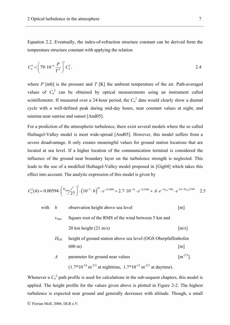
Equation 2.2. Eventually, the index-of-refraction structure constant can be derived form the
temperature structure constant with applying the relation
22 6 2n T279 10 PC C
T−⎛ ⎞= ⋅⎜ ⎟
⎝ ⎠. 2.4
where P [mb] is the pressure and T [K] the ambient temperature of the air. Path-averaged
values of Cn2 can be obtained by optical measurements using an instrument called
scintillometer. If measured over a 24-hour period, the Cn2 data would clearly show a diurnal
cycle with a well-defined peak during mid-day hours, near constant values at night, and
minima near sunrise and sunset [And05].
For a prediction of the atmospheric turbulence, there exist several models where the so called
Hufnagel-Valley model is most wide-spread [And05]. However, this model suffers from a
severe disadvantage. It only creates meaningful values for ground station locations that are
located at sea level. If a higher location of the communication terminal is considered the
influence of the ground near boundary layer on the turbulence strength is neglected. This
leads to the use of a modified Hufnagel-Valley model proposed in [Gig04] which takes this
effect into account. The analytic expression of this model is given by
( ) ( )GSGS
210 1007002 5 1000 16 1500rms
n ( ) 0.00594 10 2.7 1027h HHh hvC h h e e A e e− −−− − − −⎛ ⎞= ⋅ ⋅ ⋅ ⋅ + ⋅ ⋅ + ⋅ ⋅⎜ ⎟
⎝ ⎠2.5
with h observation height above sea level [m]
vrms Square root of the RMS of the wind between 5 km and
20 km height (21 m/s) [m/s]
HGS height of ground station above sea level (OGS Oberpfaffenhofen
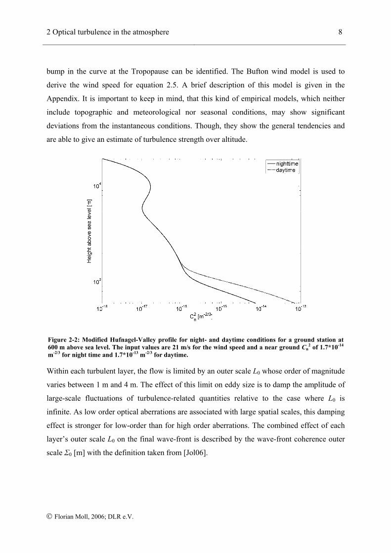
600 m) [m]
A parameter for ground near values [m-2/3].
(1.7*10-14 m-2/3 at nighttime, 1.7*10-13 m-2/3 at daytime).
Whenever a Cn2 path profile is used for calculations in the sub-sequent chapters, this model is
applied. The height profile for the values given above is plotted in Figure 2-2. The highest
turbulence is expected near ground and generally decreases with altitude. Though, a small
2 Optical turbulence in the atmosphere 8
© Florian Moll, 2006; DLR e.V.
bump in the curve at the Tropopause can be identified. The Bufton wind model is used to
derive the wind speed for equation 2.5. A brief description of this model is given in the
Appendix. It is important to keep in mind, that this kind of empirical models, which neither
include topographic and meteorological nor seasonal conditions, may show significant
deviations from the instantaneous conditions. Though, they show the general tendencies and
are able to give an estimate of turbulence strength over altitude.
Figure 2-2: Modified Hufnagel-Valley profile for night- and daytime conditions for a ground station at 600 m above sea level. The input values are 21 m/s for the wind speed and a near ground Cn
2 of 1.7*10-14 m-2/3 for night time and 1.7*10-13 m-2/3 for daytime.
Within each turbulent layer, the flow is limited by an outer scale L0 whose order of magnitude
varies between 1 m and 4 m. The effect of this limit on eddy size is to damp the amplitude of
large-scale fluctuations of turbulence-related quantities relative to the case where L0 is
infinite. As low order optical aberrations are associated with large spatial scales, this damping
effect is stronger for low-order than for high order aberrations. The combined effect of each
layer’s outer scale L0 on the final wave-front is described by the wave-front coherence outer
scale Σ0 [m] with the definition taken from [Jol06].
2 Optical turbulence in the atmosphere 9
© Florian Moll, 2006; DLR e.V.
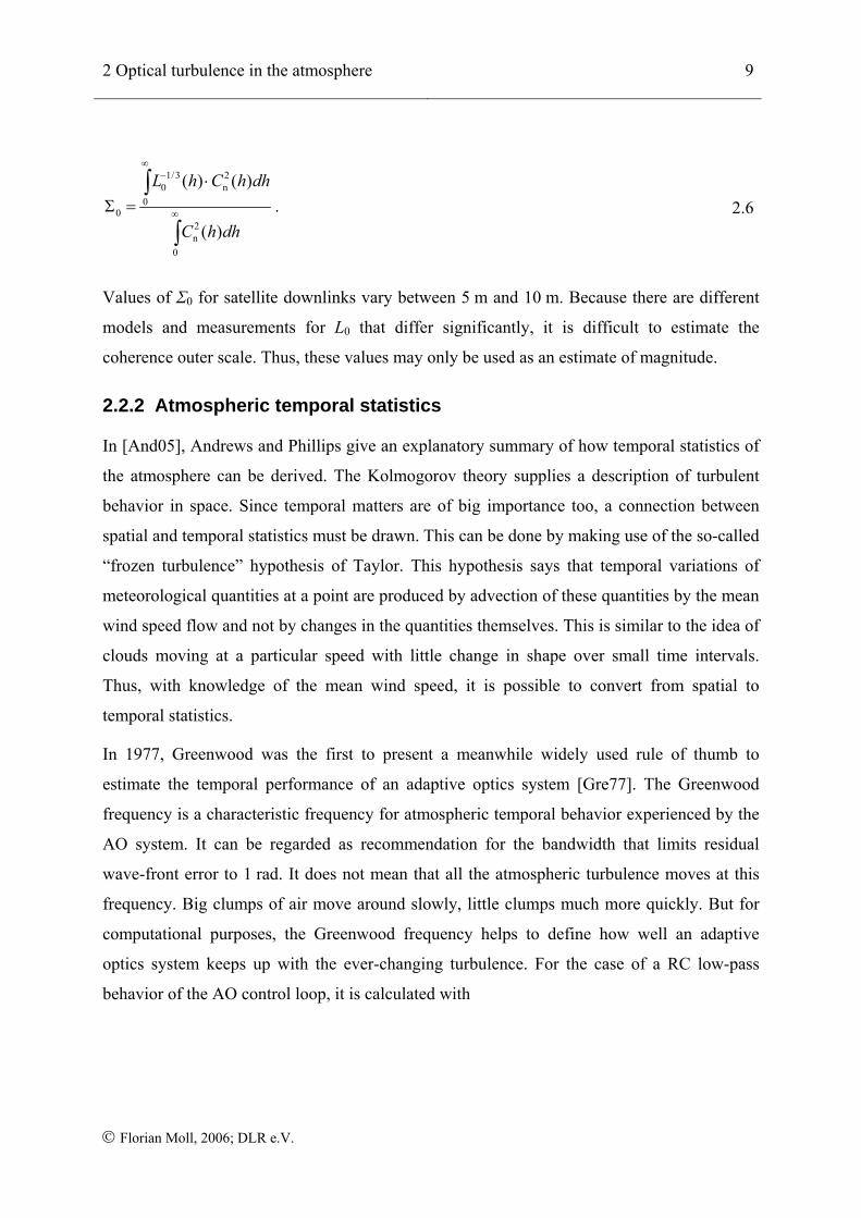
1/3 20 n
00
2n
0
( ) ( )
( )
L h C h dh
C h dh
∞−
∞
⋅Σ =
∫
∫. 2.6
Values of Σ0 for satellite downlinks vary between 5 m and 10 m. Because there are different
models and measurements for L0 that differ significantly, it is difficult to estimate the
coherence outer scale. Thus, these values may only be used as an estimate of magnitude.
2.2.2 Atmospheric temporal statistics
In [And05], Andrews and Phillips give an explanatory summary of how temporal statistics of
the atmosphere can be derived. The Kolmogorov theory supplies a description of turbulent
behavior in space. Since temporal matters are of big importance too, a connection between
spatial and temporal statistics must be drawn. This can be done by making use of the so-called
“frozen turbulence” hypothesis of Taylor. This hypothesis says that temporal variations of
meteorological quantities at a point are produced by advection of these quantities by the mean
wind speed flow and not by changes in the quantities themselves. This is similar to the idea of
clouds moving at a particular speed with little change in shape over small time intervals.
Thus, with knowledge of the mean wind speed, it is possible to convert from spatial to
temporal statistics.
In 1977, Greenwood was the first to present a meanwhile widely used rule of thumb to
estimate the temporal performance of an adaptive optics system [Gre77]. The Greenwood
frequency is a characteristic frequency for atmospheric temporal behavior experienced by the
AO system. It can be regarded as recommendation for the bandwidth that limits residual
wave-front error to 1 rad. It does not mean that all the atmospheric turbulence moves at this
frequency. Big clumps of air move around slowly, little clumps much more quickly. But for
computational purposes, the Greenwood frequency helps to define how well an adaptive
optics system keeps up with the ever-changing turbulence. For the case of a RC low-pass
behavior of the AO control loop, it is calculated with
2 Optical turbulence in the atmosphere 10
© Florian Moll, 2006; DLR e.V.
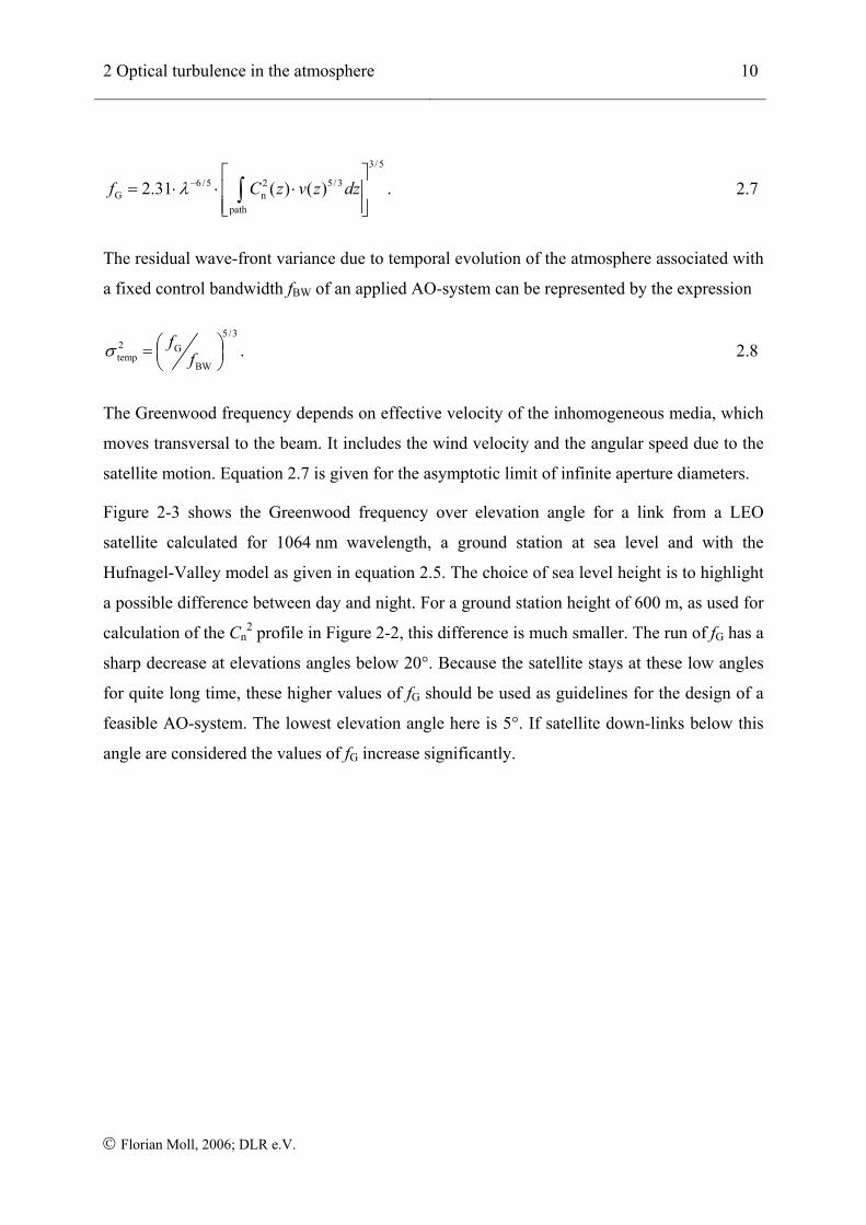
3/5
6 /5 2 5/3G n
path
2.31 ( ) ( )f C z v z dzλ−⎡ ⎤
= ⋅ ⋅ ⋅⎢ ⎥⎢ ⎥⎣ ⎦∫ . 2.7
The residual wave-front variance due to temporal evolution of the atmosphere associated with
a fixed control bandwidth fBW of an applied AO-system can be represented by the expression
5/32 Gtemp
BW
ffσ ⎛ ⎞= ⎜ ⎟
⎝ ⎠. 2.8
The Greenwood frequency depends on effective velocity of the inhomogeneous media, which
moves transversal to the beam. It includes the wind velocity and the angular speed due to the
satellite motion. Equation 2.7 is given for the asymptotic limit of infinite aperture diameters.
Figure 2-3 shows the Greenwood frequency over elevation angle for a link from a LEO
satellite calculated for 1064 nm wavelength, a ground station at sea level and with the
Hufnagel-Valley model as given in equation 2.5. The choice of sea level height is to highlight
a possible difference between day and night. For a ground station height of 600 m, as used for
calculation of the Cn2 profile in Figure 2-2, this difference is much smaller. The run of fG has a
sharp decrease at elevations angles below 20°. Because the satellite stays at these low angles
for quite long time, these higher values of fG should be used as guidelines for the design of a
feasible AO-system. The lowest elevation angle here is 5°. If satellite down-links below this
angle are considered the values of fG increase significantly.
2 Optical turbulence in the atmosphere 11
© Florian Moll, 2006; DLR e.V.
Figure 2-3: Greenwood frequency over elevation angle of satellite overpass for night and daytime conditions of turbulence at a wavelength of 1064 nm and the turbulence profile in Figure 2-2.
2.3 Distorted wave-fronts
2.3.1 Description of wave-front
For a better understanding of the problems that arise with distorted wave-fronts, it is useful to
explain their definition first. Wave-fronts define surfaces of constant optical path length and
phase as illustrated with two rays originating from a point source in Figure 2-4. If the point
source is moved to infinity the curved wave-front morphs to a plane wave and the
corresponding light beam is said to be collimated. The spherical wave-front and flat wave-
front are ideal constructions against which other wave-fronts can be compared.
2 Optical turbulence in the atmosphere 12
© Florian Moll, 2006; DLR e.V.
Figure 2-4: Illustration of a spherical wave-front originating from a point source (PS). The wave-front is illustrated by the phase relationship between two rays [Gea95].
An aberrated wave-front (AWF) can be described by comparing it to an ideal wave-front
which forms the reference wave-front in that case. In [Gea95], it is stated to construct the
wave-front with its vertex tangent to the exit pupil of the optical system, and its center of
curvature coincident with the ideal image point in the image plane as illustrated in Figure 2-5.
For each point in the exit pupil, the optical path difference (OPD) is measured between the
spherical reference surface and the aberrated wave-front along the radius of the reference
surface. A function W(x,y) for the OPD is obtained over the pupil, depicted in Figure 2-5,
which can be used as the description of the aberrated wave-front.
Figure 2-5: Exit pupil aberration W(x,y). The optical path difference of the spherical reference surface (SRS) and the aberrated wave-front (AWF) defines the function W(x,y), usually with dimension in wavelengths or meter [Gea95].
2 Optical turbulence in the atmosphere 13
© Florian Moll, 2006; DLR e.V.
Usually wave-fronts are described by using special polynomials. One possibility often applied
in practice when dealing with measurements is the use of Zernike polynomials which are
described in Chapter 2.3.4.
2.3.2 Origin of wave-front distortions
The index-of-refraction fluctuations described by the Cn2 along the propagation path cause the
distortion of the propagating wave-front. Because the distortion is dependent on the
turbulence strength, it is expected to be more severe for a propagation path at low than at high
elevation angles. Considering LEO down-links, the satellite stays most of the time at low
elevation which makes the propagation path long and the turbulence strong. Thus, the wave-
front is considered to suffer from very high distortions.
Simplified, it is possible to say that the wave-front distortions are near field effects and
scintillations are far field effects of the same origin. However, for long propagation distances
this simplification may be too coarse. Additional effects like beam broadening and beam
wander can occur [Gig04], but theses are not of interest here.
2.3.3 Fried parameter and focus spot size
For an assessment of wave-front distortions it is necessary to define a suitable metric. Under
ideal conditions, the wave in the aperture is focused to form a well-shaped spot. The
corresponding intensity in the focal plane forms an Airy pattern whose diameter is given by
[Hec05]
Airy 2.44 fdDλ⋅
= ⋅ , 2.9
with f [m] the focal length of the optical system, λ [m] the wavelength and D [m] the aperture
diameter of the receiver telescope. Under ideal conditions, the incident optical field is uniform
over the receiver aperture in intensity and phase. But after a wave has propagated trough the
atmosphere it exhibits less spatial coherence and the intensity distribution is not uniform any
more. These effects prevent the wave from being properly focused. Fried introduced in
[Fri67] the coherence diameter r0 (also called the Fried parameter) as a statistical measure of
spatial coherence for waves distorted by turbulence. The Fried parameter became an
important matter especially in the field of astronomy as a measure of seeing of a telescope
2 Optical turbulence in the atmosphere 14
© Florian Moll, 2006; DLR e.V.
under the influence of atmospheric turbulence. If r0 is smaller than the telescope aperture, the
mean diameter at full width half maximum (FWHM) of the focal spot dFWHM [m] will increase
according to [Gli97a]
FWHM0
0.98 fdrλ⋅
= ⋅ . 2.10
The spread of the focal spot defined by equation 2.10 represents actually a spread averaged
over a long time period. The instantaneous spot diameter observed at a given instant may be
smaller, but larger than the ideal Airy-shaped one. Its centroid (or center-of-gravity) may be
randomly shifted from the optical axis: it is observed that the spot “dances” in the focal plane
at the rate of atmospheric perturbations. Additionally, the focal spot exhibits intensity
speckles that are related to the incident field by a Fourier transform. Typical focal spots are
illustrated in Figure 2-6 for different r0 relative to the receiver aperture. The dashed circles for
the last two images show the long-term spot diameters which define the distribution area of
the received optical power [Per05].
Figure 2-6: Short-term spots in the focal plane under different levels of turbulence. The dashed circles for the last two images show the long-term spot diameter [Per05].
For an infinite plane wave, as it appears in astronomical applications and satellite downlinks,
the Fried parameter is usually estimated by [And05]
3/52 2
0 n00.42 ( )
Lr k C z dz
−⎡ ⎤= ⋅ ⋅⎢ ⎥⎣ ⎦∫ . 2.11
Here, k is the circular wave number with dimension [m-1] and z [m] is the variable of
integration along the propagation path with length L [m]. Thus, the Fried parameter depends
on the turbulence strength and length of propagation path and on the wavelength. That means,
2 Optical turbulence in the atmosphere 15
© Florian Moll, 2006; DLR e.V.
for a given communication scenario, the signal degradation caused by turbulence decreases
with increasing wavelength.
2.3.4 Representation of wave-fronts with Zernike polynomials
For the understanding of the forthcoming application of angle-of-arrival (AoA) measurements
of the wave-front it is useful to introduce the method of Zernike mode expansion of an
arbitrary wave-front as it is recommended in [Nol76]. For a circular aperture without
obstruction, using polar coordinates (r, γ), the Zernike polynomials are defined here by
even
2 cos( ) ( 0)
1 ( ) 2 sin( ) ( 0)1 ( 0)
mj l
m m
Z l R r m mm
γ
γ
⎧ ≠⎪⎪= + ⋅ ⋅ ≠⎨⎪ =⎪⎩
2.12
where
[ ] [ ]( ) / 2
2
0
( 1) ( )!( ) .! ( ) / 2 ! ( ) / 2 !
sl mm l sl
s
l sR r rs l m s l m s
−−
=
− −=
+ − − −∑ 2.13
The values of l and m are always integer integral and satisfy m ≤ l, l - |m| = even. The index j
is a mode ordering number and is a function of l and m. A table with the first 15 Zernike
modes along with the classical aberration with which they are associated can be found in the
Appendix. The definition in equation 2.12 gives a logical ordering of the modes. A
polynomial expansion of an arbitrary wave-front over a circle is given by
( , ) ( , )j jj
r a Z rϕ γ γ=∑ 2.14
where aj [waves] are the coefficients of Zernike mode expansion.
The first mode is the phase piston which is not important if the main goal for wave-front
correction is to form a small spot or to couple into a single mode fiber, respectively. Problems
with varying piston may arise if superposition of the received wave with a local oscillator for
coherent detection techniques is needed. The second and third modes are the tip and tilt
modes which describe the changing angle-of-arrival in x- and y-direction. The temporal
behavior of these two modes can be measured with short-time exposure images of a focus
2 Optical turbulence in the atmosphere 16
© Florian Moll, 2006; DLR e.V.
camera. Doing so, the Zernike modes are not measured directly but rather the deviation of the
center-of-gravity from a reference in the image plane. The angle-of-arrival metrics are
discussed in the next chapter.
2.3.5 G-tilt and Z-tilt: Angle-of-arrival
2.3.5.1 Definition of the angle-of-arrival
In the absence of scintillation the G-tilt (center-of-gravity tilt) is the direction associated with
the centroid of a target. Quadrant detectors and centroid trackers measure something that
strongly resembles the G-tilt. The Z-tilt (Zernike tilt) is the direction that is defined by the
normal to a plane that best fits the wave-front distortion. The tilts associated with the two
lower order Zernike polynomials are precisely equal to the two components of the Z-tilt
[Tyl94].
The measurement of the image intensity centroid can be used to obtain an estimate of the
wave-front slope. The centroid, or first-order moment Mx, of the image intensity I(x,y) with
respect to the x direction in the image, is related to the partial derivative of the wave-front in
the aperture by
imagex
apertureimage
( , )
( , )
I x y x dx dyM du dv
uI x y dx dyϕ∂
= =∂
∫∫∫∫∫∫
. 2.15
Where φ(u,v) is the phase in the aperture plane with coordinates u [m] and v [m]. Taking the
derivatives of the Zernike polynomials results in
x 2 82 ...M a a∝ + + ., 2.16
where a2 is the tilt term and a8 is the coma term of the Zernike mode expansion. As the
optimal estimate of the wave-front slope is given by a2 alone, the image centroid is not the
best measure. However, the influence of the coma term is relatively small [Gli97].
The measurement of the G-tilt comes out to be simple because it can be directly derived from
the center-of-gravity of a short-time-exposure image. But, the Z-tilt is more interesting
because it can be used for a Zernike modal expansion of the wave-front. Tyler proved that for
2 Optical turbulence in the atmosphere 17
© Florian Moll, 2006; DLR e.V.
low frequencies of angle-of-arrival Z- and G-tilt are identical [Tyl94] and thus, the center-of-
gravity method is also applicable for modal expansion in this limited interval.
In general, the power spectral density (PSD) of a particular metric can be derived from its
autocorrelation function (ACF) [And05]. In the following, the analytical expressions for the
PSD of the Z- and G-tilt taken from [Tyl94] are given and evaluated for an example scenario.
In Chapter 5, these expressions will be compared to turbulence measurements with the focus
camera.
2.3.5.2 Angle-of-arrival spectral power density for Z-tilt
The one axis angle-of-arrival PSD of the Z-tilt is calculated with
1 3 14 3 2 11/3Z n n Z
1 ( ) 0.251 sec( ) ( ) ( )2
f D f C h dh F fψ ν ν− −Φ = ⋅ ⋅∫ , 2.17
where
1 11 32
Z 220
( ) ( )1qF p J p q dq
qπ=
−∫ . 2.18
Furthermore, equation 2.17 contains the normalization
nVD
ν = 2.19
and ψ [°], the zenith angle of observation direction. The wind speed V [m/s] is assumed to be
constant here. The factor one half is due to the handling of only one axis. It can be seen that
equation 2.18 contains the Bessel function of second kind. With
[(1 2 )]( )!
p
iqJ q
p≈ 2.20
it is possible to approximate equation 2.17 with two asymptotes, for low and high frequencies.
For low frequencies the PSD takes the form
2 Optical turbulence in the atmosphere 18
© Florian Moll, 2006; DLR e.V.
1 3 2 3 2 1/3Z n n
1 ( ) 0.804 sec( ) ( )2
f D f C h dhψ ν− − −Φ = ⋅ ∫ . 2.21
Here, a two-third power law is observable which goes along with the statements in [Con95].
For high frequencies it takes the form
1 3 17 3 2 14/3Z n n
1 ( ) 0.0140 sec( ) ( )2
f D f C h dhψ ν− −Φ = ⋅ ∫ , 2.22
where now a seventeen-third exponent is observed. The knee frequency has linear behavior
and is determined by
K n0.44f ν= ⋅ . 2.23
This frequency may be used to determine the effective wind speed.
It must be mentioned that for high frequencies the resulting asymptotes for the Z-tilt are
different in [Tyl94] and [Con95]. The first one predicts a seventeen-third behavior whereas
the second one results in an eleven-third behavior.
2.3.5.3 Angle-of-arrival spectral power density for G-tilt
The G-tilt angle-of-arrival PSD has the form
1 3 8 3 2 5/3G n n G
1 ( ) 0.155 sec( ) ( ) ( )2
f D f C h dh F fψ ν ν− −Φ = ⋅ ⋅∫ , 2.24
where
1 5 32
G 120
( ) ( )1xF y J y x dx
xπ=
−∫ . 2.25
Again, with equation 2.20, the PSD of G-tilt for low frequencies is approximated with the
exponential asymptote
2 Optical turbulence in the atmosphere 19
© Florian Moll, 2006; DLR e.V.
1 3 2 3 2 1/3G n n
1 ( ) 0.804 sec( ) ( )2
f D f C h dhψ ν− − −Φ = ⋅ ∫ 2.26
which has exactly the same form as the Z-tilt PSD for low frequencies. However, for high
frequencies it is different and takes the form
1 3 11 3 2 8/3Z n n
1 ( ) 0.0110 sec( ) ( )2
f D f C h dhψ ν− −Φ = ⋅ ∫ . 2.27
The knee frequency is now calculated with
K n0.24f ν= ⋅ . 2.28
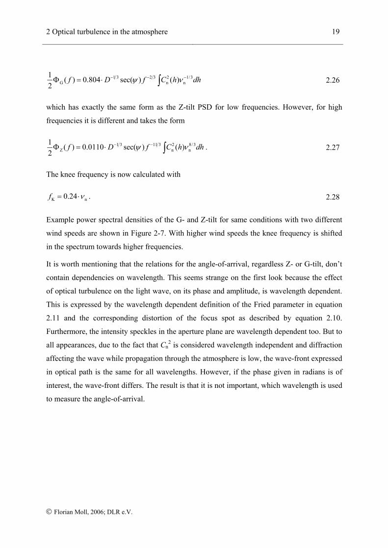
Example power spectral densities of the G- and Z-tilt for same conditions with two different
wind speeds are shown in Figure 2-7. With higher wind speeds the knee frequency is shifted
in the spectrum towards higher frequencies.
It is worth mentioning that the relations for the angle-of-arrival, regardless Z- or G-tilt, don’t
contain dependencies on wavelength. This seems strange on the first look because the effect
of optical turbulence on the light wave, on its phase and amplitude, is wavelength dependent.
This is expressed by the wavelength dependent definition of the Fried parameter in equation
2.11 and the corresponding distortion of the focus spot as described by equation 2.10.
Furthermore, the intensity speckles in the aperture plane are wavelength dependent too. But to
all appearances, due to the fact that Cn2 is considered wavelength independent and diffraction
affecting the wave while propagation through the atmosphere is low, the wave-front expressed
in optical path is the same for all wavelengths. However, if the phase given in radians is of
interest, the wave-front differs. The result is that it is not important, which wavelength is used
to measure the angle-of-arrival.
2 Optical turbulence in the atmosphere 20
© Florian Moll, 2006; DLR e.V.
Figure 2-7: Power spectral densities for G- and Z-tilts (blue and black line) for two wind speeds. The receiver aperture is 40 cm, the propagation path is 1 km with a Cn
2 of 1*10-13 m2/3.
2.3.6 Expected aberrations and wave-front tilt
The expected deformation of the wave-front gives an estimate for the required stroke for a
deformable mirror (DM) and a tip-tilt mirror (TM). The stroke for each actuator of a DM is
determined by finding the maximum amount of atmospheric wave-front error across the
aperture. In that case it is assumed that the global tilt is corrected by a dedicated tip-tilt mirror.
The tip-tilt corrected standard deviation σWF [rad] of atmospheric turbulence across the
aperture D is calculated with [Nol76]
56
WF0
0.366 Drσ ⎛ ⎞= ⋅⎜ ⎟
⎝ ⎠. 2.29
The standard deviation of the atmospheric tilt σtilt [rad] over the aperture of the telescope
primary mirror can be estimated with an expression given in [Tys00].
2 Optical turbulence in the atmosphere 21
© Florian Moll, 2006; DLR e.V.
( )5
23
tilt0
0.184 Dr D
λσ ⎛ ⎞= ⋅⎜ ⎟⎝ ⎠
. 2.30
These rules of thumb are practicable to estimate the present wave-front distortions. Although,
equation 2.30 seems to contain dependence of σtilt on wavelength, this can be disproved by
inserting equation 2.11 into 2.30. However, the tip-tilt corrected wave-front aberrations given
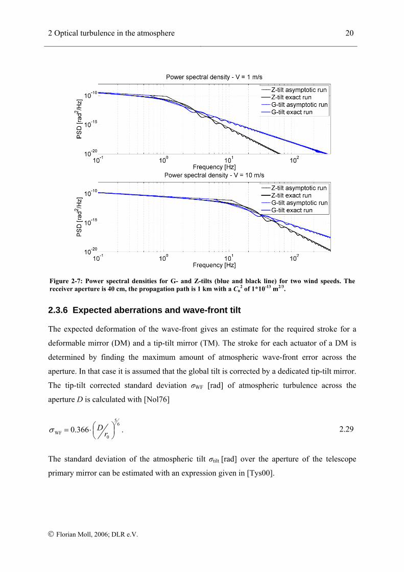
in dimension [rad], like in equation 2.29, are wavelength dependent. Figure 2-8 illustrates
how the wave-front characteristics in equation 2.29 and 2.30 change with increasing r0 and
different apertures for a fix wavelength of 1064 nm.
Figure 2-8: Tip-tilt and wave-front standard deviation for λ = 1064 nm and two aperture sizes. The standard deviation of tip-tilt corrected wave-front is wavelength dependent. However, the standard deviation of angle-of-arrival is not. Considering a real LEO satellite down-link scenario, r0 is expected to vary between 10 mm and 200 mm for different elevation angles, respectively.
2.4 Scintillation effects
This chapter gives a brief introduction into the problems associated with intensity
fluctuations. The fluctuation in received intensity from propagation through turbulence is
described as scintillation. The term scintillation is applied to various phenomena, including
the temporal variation in received intensity (such as the twinkling of a star) or the spatial
2 Optical turbulence in the atmosphere 22
© Florian Moll, 2006; DLR e.V.
variation in received intensity within a receiver aperture. From the definition of log amplitude,
it is seen that the statistics of intensity are determined by those log amplitude [Smi96].
Thus, after a certain propagation distance, the incident wave-front not only fluctuates in phase
but also in amplitude. That is, the intensity in the pupil plane is not uniform, neither spatially
nor temporally. This may cause problems in wave-front sensing, for example with a Shack-
Hartmann sensor when sub-apertures are not illuminated over sensitivity threshold of the
sensor or when in scenarios with strong turbulence branch points emerge. Furthermore, large
dynamic is needed to avoid saturation of the sensor.
Scintillation is more severe for longer propagation through the turbulent medium than it is for
short distances. Therefore stronger fluctuations are expected for optical satellite downlinks
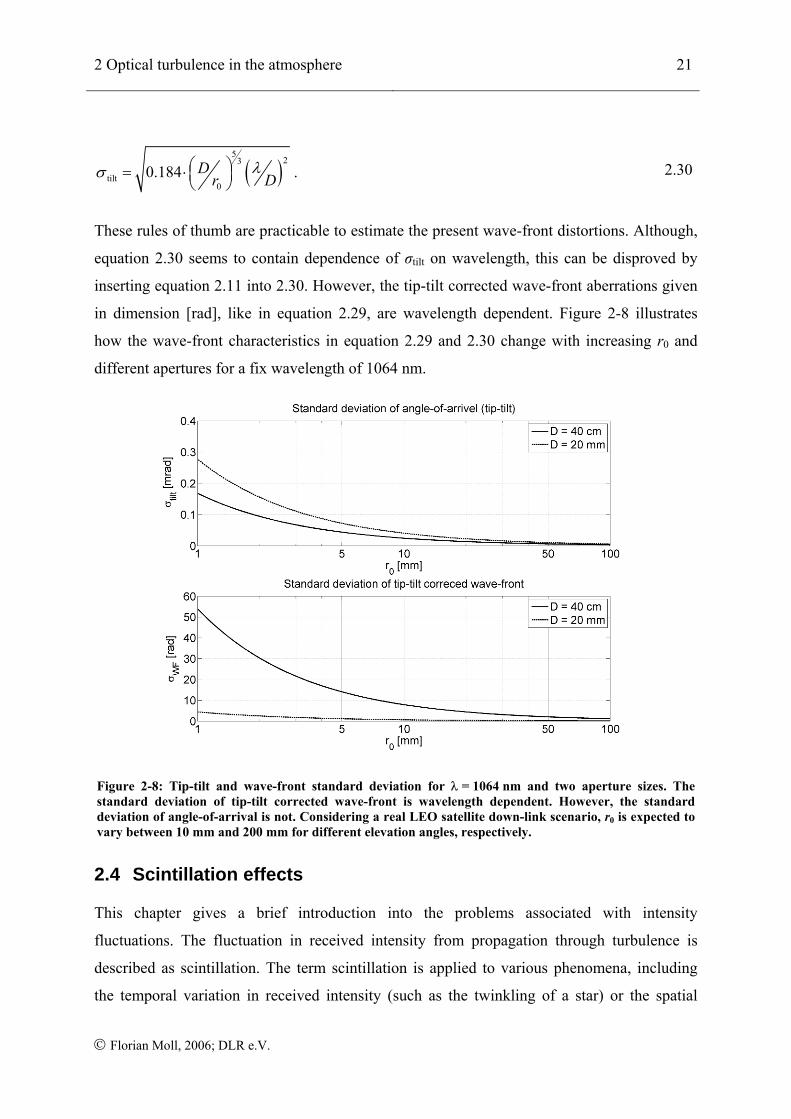
with lower elevation angles. Figure 2-9 gives an example of the dependency of the intensity
probability density function (PDF) of a point receiver on the link elevation angle. The graph is
based on data derived from measurements during an optical satellite down-link (KIODO
experiment [Per07] ) and shows two effects. The one is the shift of the PDF with higher
elevation to higher intensity which means lower probability of fades. The other is the decrease
in intensity (digital numbers) caused by the longer link distance.
Figure 2-9: Probability distribution of the received intensity (point receiver) for several elevation angles. These data have been measured during the KIODO experiment which consisted in an optical downlink from a Japanese LEO satellite, λ = 847 nm. The intensity was measured by camera in digital numbers (DN) [Per07].
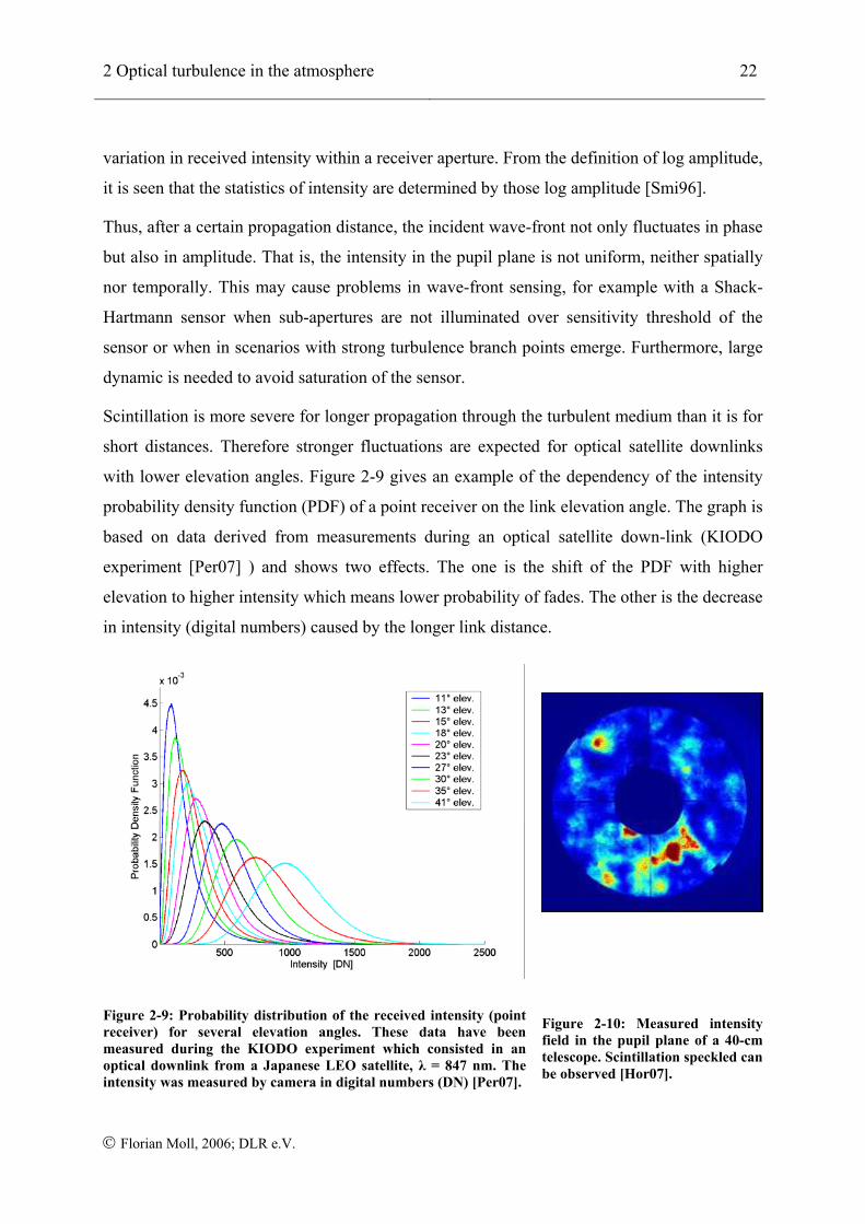
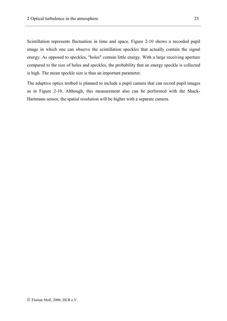
Figure 2-10: Measured intensity field in the pupil plane of a 40-cm telescope. Scintillation speckled can be observed [Hor07].
2 Optical turbulence in the atmosphere 23
© Florian Moll, 2006; DLR e.V.
Scintillation represents fluctuation in time and space. Figure 2-10 shows a recorded pupil
image in which one can observe the scintillation speckles that actually contain the signal
energy. As opposed to speckles, "holes" contain little energy. With a large receiving aperture
compared to the size of holes and speckles, the probability that an energy speckle is collected
is high. The mean speckle size is thus an important parameter.
The adaptive optics testbed is planned to include a pupil camera that can record pupil images
as in Figure 2-10. Although, this measurement also can be performed with the Shack-
Hartmann sensor, the spatial resolution will be higher with a separate camera.
3 Adaptive optics in free space optical communications 24
© Florian Moll, 2006; DLR e.V.
3 Adaptive optics in free space optical communications
3.1 Principle of adaptive optics systems
Accompanying the testbed development, research of how a usual AO system is working was
necessary, and what influence it may have on communication performance. The task of the
AO system is to correct the deformations of the incoming wave-front. There are several
different approaches how this goal can be achieved but in general, all follow the same way.
The entrance pupil of the optical system is imaged on a deformable mirror that, in the ideal
case, forms an inversion of the aberrated wave-front. Behind the DM, the beam is guided to a
wave-front sensor (WFS) that measures its shape. Based on this measurement, a control
system outputs the steering signals for the DM which flattens the wave-front. This wave-front,
in turn, is measured by the WFS again. That way, the AO control loop is closed. Additionally
to the DM, a tip-tilt mirror (TM) is located in a conjugate pupil before to pre-correct for the
angle-of-arrival. Eventually, a plane wave is generated and a nice focus can be formed as
illustrated in Figure 3-1. Here, it is shown how the aberrated wave-front is formed by the DM
and part of the signal is split and guided to the WFS for measuring. In [Tys00], Tyson gives a
very good illustration of how the individual elements of the AO system work together. He
considers the wave-front sensor as the eyes of the system, whereas the control computer is the
brain that produces commands for the hands, the deformable and tip-tilt mirror.
An example system applied in practice is shown in Figure 3-2. It depicts the main elements of
the optical system of ALFA (Adaptive optics with a Laser For Astronomy), the adaptive
optics system of the 3.5 m astronomical telescope on Calar Alto, Spain. A TM is used for
correction of image motion. The first focusing mirror images the telescope pupil on the DM
which reflects the beam to a second focusing mirror that reimages the telescope focus.
Finally, a beam splitter (BS) reflects a beam to the science camera and transmits a beam to the
wave-front sensor arm. Both illustrations point out that in most cases of AO systems, the light
beam does not incident onto the DM at a 90° angle but a lower one. Many AO systems in
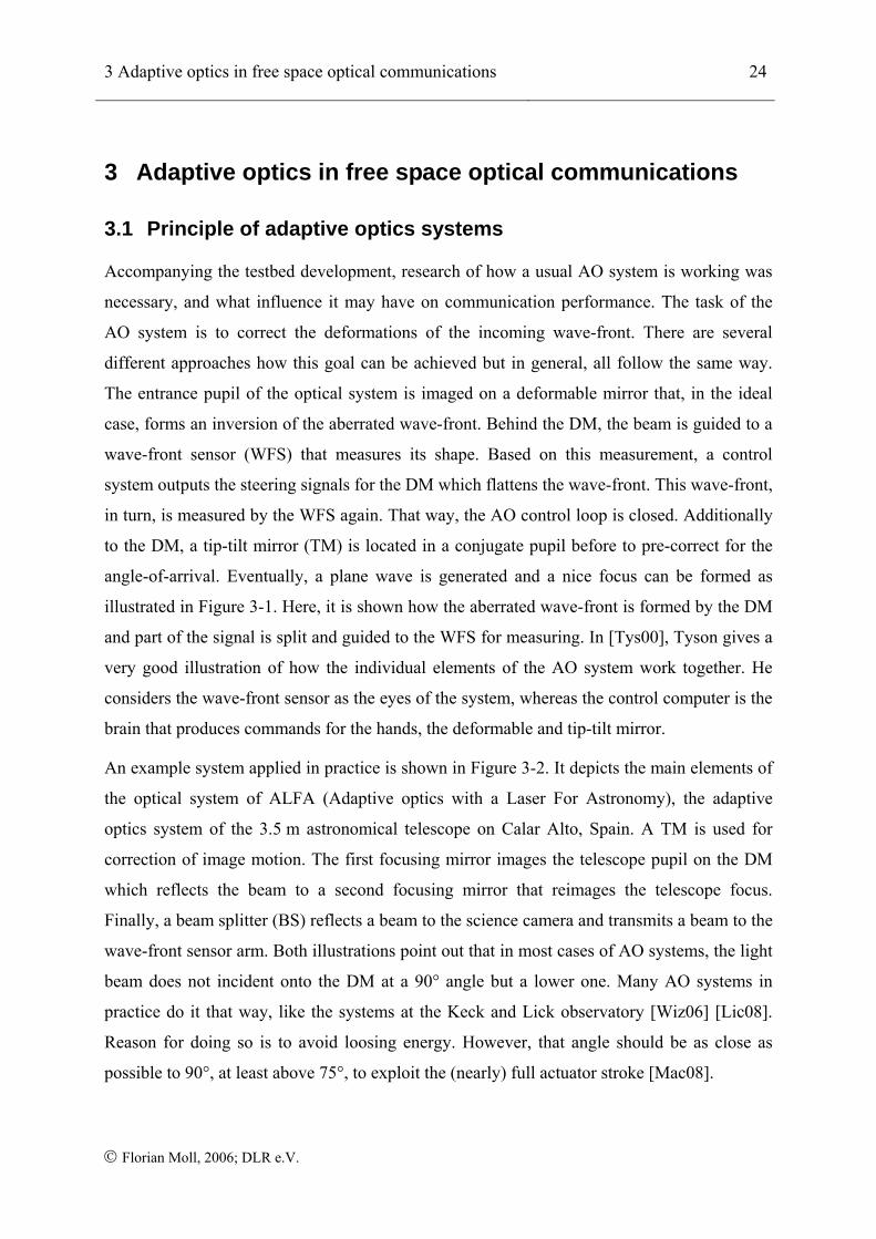
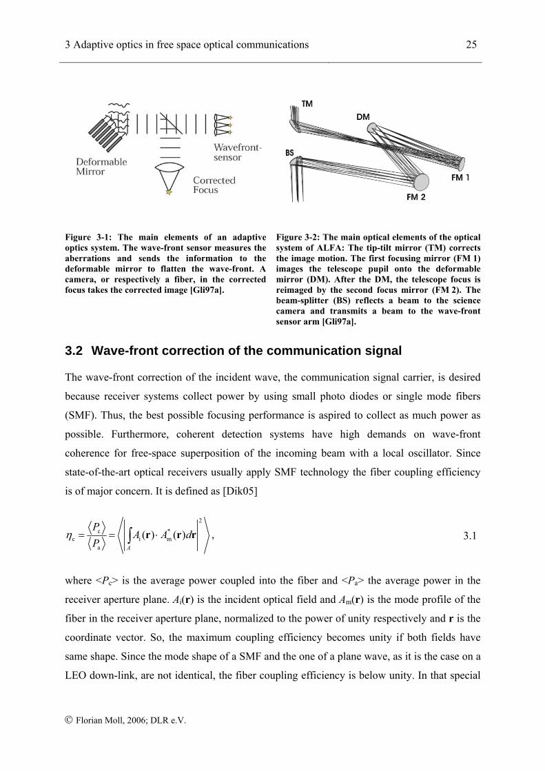
practice do it that way, like the systems at the Keck and Lick observatory [Wiz06] [Lic08].
Reason for doing so is to avoid loosing energy. However, that angle should be as close as
possible to 90°, at least above 75°, to exploit the (nearly) full actuator stroke [Mac08].
3 Adaptive optics in free space optical communications 25
© Florian Moll, 2006; DLR e.V.
Figure 3-1: The main elements of an adaptive optics system. The wave-front sensor measures the aberrations and sends the information to the deformable mirror to flatten the wave-front. A camera, or respectively a fiber, in the corrected focus takes the corrected image [Gli97a].
Figure 3-2: The main optical elements of the optical system of ALFA: The tip-tilt mirror (TM) corrects the image motion. The first focusing mirror (FM 1) images the telescope pupil onto the deformable mirror (DM). After the DM, the telescope focus is reimaged by the second focus mirror (FM 2). The beam-splitter (BS) reflects a beam to the science camera and transmits a beam to the wave-front sensor arm [Gli97a].
3.2 Wave-front correction of the communication signal
The wave-front correction of the incident wave, the communication signal carrier, is desired
because receiver systems collect power by using small photo diodes or single mode fibers
(SMF). Thus, the best possible focusing performance is aspired to collect as much power as
possible. Furthermore, coherent detection systems have high demands on wave-front
coherence for free-space superposition of the incoming beam with a local oscillator. Since
state-of-the-art optical receivers usually apply SMF technology the fiber coupling efficiency
is of major concern. It is defined as [Dik05]
2
c *c i m
a
( ) ( )A
PA A d
Pη = = ⋅∫ r r r , 3.1
where <Pc> is the average power coupled into the fiber and <Pa> the average power in the
receiver aperture plane. Ai(r) is the incident optical field and Am(r) is the mode profile of the
fiber in the receiver aperture plane, normalized to the power of unity respectively and r is the
coordinate vector. So, the maximum coupling efficiency becomes unity if both fields have
same shape. Since the mode shape of a SMF and the one of a plane wave, as it is the case on a
LEO down-link, are not identical, the fiber coupling efficiency is below unity. In that special
3 Adaptive optics in free space optical communications 26
© Florian Moll, 2006; DLR e.V.
it amounts 82 % [Dik05]. This value is the maximum fiber coupling efficiency without any
wave-front aberrations for an incident plane wave.
Since there is no analytical expression known that relates the wave-front standard deviation to
the fiber coupling efficiency, as an alternative the metric of the Strehl ratio is used. This is
closely related to the fiber coupling efficiency and even equal for the case of an incident wave
with Gaussian distribution as it is the case by coupling from SMF to SMF through an arbitrary
optical system [Wag82].
The Strehl ratio SSR can be calculated with the Maréchal approximation [Mah83]
2SR WFexp( )S σ= − . 3.2
This metric can also be used to evaluate the overall system performance when focusing on a
diode or fiber face. The loss due to mode mismatch is neglected here. The relation between
Strehl ratio and wave-front aberration is inverse which means low aberrations give high Strehl
ratios. Noll [Nol76] presented a connection between the number of corrected Zernike modes
(as numbered in the Appendix) and the residual wave-front error where the formulas for
correction of the first ten modes are listed in Table 3-1. For higher modes (j > 10) the
expression
2 3 / 2 5/3WF, 00.2944 ( / )j j D rσ −= ⋅ 3.3
may be used where j is the Zernike mode index.
2 5/3WF,1 01.0299 ( / )D rσ = ⋅ 2 5/3
WF,6 00.0648 ( / )D rσ = ⋅
2 5/3WF,2 00.582 ( / )D rσ = ⋅ 2 5/3
WF,7 00.0587 ( / )D rσ = ⋅
2 5/3WF,3 00.134 ( / )D rσ = ⋅ 2 5/3
WF,8 00.0525 ( / )D rσ = ⋅
2 5/3WF,4 00.111 ( / )D rσ = ⋅ 2 5/3
WF,9 00.0463 ( / )D rσ = ⋅
2 5/3WF,5 00.0880 ( / )D rσ = ⋅ 2 5/3
WF,10 00.0401 ( / )D rσ = ⋅
Table 3-1: Zernike-Kolmogorov residual errors σWF2 for the first ten modes dependent on Fried
parameter r0 and aperture size D [Nol76].
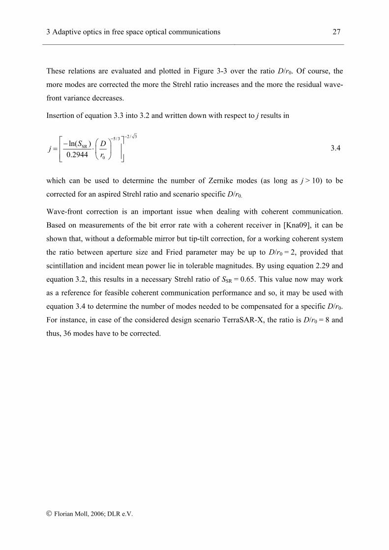
3 Adaptive optics in free space optical communications 27
© Florian Moll, 2006; DLR e.V.
These relations are evaluated and plotted in Figure 3-3 over the ratio D/r0. Of course, the
more modes are corrected the more the Strehl ratio increases and the more the residual wave-
front variance decreases.
Insertion of equation 3.3 into 3.2 and written down with respect to j results in
2/ 35/3
SR
0
ln( )0.2944
S Djr
−−⎡ ⎤⎛ ⎞−⎢ ⎥= ⋅⎜ ⎟⎢ ⎥⎝ ⎠⎣ ⎦
3.4
which can be used to determine the number of Zernike modes (as long as j > 10) to be
corrected for an aspired Strehl ratio and scenario specific D/r0.
Wave-front correction is an important issue when dealing with coherent communication.
Based on measurements of the bit error rate with a coherent receiver in [Kna09], it can be
shown that, without a deformable mirror but tip-tilt correction, for a working coherent system
the ratio between aperture size and Fried parameter may be up to D/r0 = 2, provided that
scintillation and incident mean power lie in tolerable magnitudes. By using equation 2.29 and
equation 3.2, this results in a necessary Strehl ratio of SSR = 0.65. This value now may work
as a reference for feasible coherent communication performance and so, it may be used with
equation 3.4 to determine the number of modes needed to be compensated for a specific D/r0.
For instance, in case of the considered design scenario TerraSAR-X, the ratio is D/r0 = 8 and
thus, 36 modes have to be corrected.
3 Adaptive optics in free space optical communications 28
© Florian Moll, 2006; DLR e.V.
Figure 3-3: Strehl ratio and wave-front variance over D/r0 for different numbers of corrected Zernike modes based on the results of [Nol76]. The run of N = 3 corresponds to the correction of piston, tip and tilt, N = 6 adds removal of defocus and astigmatism.
3.3 Requirements on the adaptive optics system
3.3.1 Spatial requirements
With knowledge of the expected wave-front aberrations the specifications of an adaptive
optics system can be developed. The maximum atmospheric tilt Mtilt that the mirror should be
able to remove is about 2.5 times the tip-tilt standard deviation [Tys00],
tilt tilt2.5M σ= ± , 3.5
where σtilt is the standard deviation of wave-front tilt given in equation 2.30. Due to the
telescope transversal magnification MT and with a factor of 0.5 because any motion of the tip-
tilt mirror results in twice the angular tilt motion of the beam, the total stroke STM of the tilt
mirror should be at least [Tys00]
3 Adaptive optics in free space optical communications 29
© Florian Moll, 2006; DLR e.V.
TM tilt tilt TTM
1 12 2
DS M M MD⎛ ⎞= =⎜ ⎟⎝ ⎠
. 3.6
Here DTM denotes the diameter of the TM covered by the light beam diameter. The aperture
ratio D/DTM equals the transversal magnification of the beam, though, only valid if the
diameter of the beam equals the diameter of the TM.
Applying a DM, the resulting Strehl ratio SSR is related to its actuator spacing rc [m] of the
deformable mirror, r0 and the constant κ which depends upon the type of deformable mirror.
For most continuous faceplate DMs, κ = 0.35 can be used. The Strehl ratio is then written as
[Tys00]
53
cSR
0exp rS rκ
⎛ ⎞⎛ ⎞= −⎜ ⎟⎜ ⎟⎜ ⎟⎝ ⎠⎝ ⎠ 3.7
and the required actuator spacing is
35
SRc 0
ln Sr r κ⎛ ⎞= ⎜ ⎟−⎝ ⎠
. 3.8
It is important to notice that this value accounts for the entrance pupil of the telescope. Thus,
if a deformable mirror is placed in the exit pupil the magnification of the preceding optical
system must be included in the calculation. The required stroke of each actuator is determined
by finding the maximum amount of atmospheric wave-front error across the aperture. It is
assumed that global tilt is corrected by a dedicated TM. The residual wave-front error σWF due
to atmospheric turbulence after tip-tilt correction across the aperture D is given in equation
2.29. The peak to peak aberration across the aperture is about 5 times the standard deviation.
If the DM moves 1 unit, the wave phase changes by 2 units. Thus the stroke SDM [rad] of the
DM is calculated with
3 Adaptive optics in free space optical communications 30
© Florian Moll, 2006; DLR e.V.
DM WF2.5S σ= ⋅ . 3.9
3.3.2 Temporal requirements
The bandwidth and acceleration of the TM can be derived from the Greenwood frequency
which is given in equation 2.7. A TM should move to its commanded position and settle down
with in its specified accuracy in less than half the time constant of the control system [Tys00].
The temporal specification for a TM can be derived by using the fundamental tracking
frequency of G-tilt fTG given in [Tyl94]. It is calculated with
1 6 1 2 2TG n0.331 sec( ) ( )f D C h V dhλ ψ− −= ⋅ ⋅ ⋅ ⋅∫ . 3.10
It is recommended that in practical system design at least four times this frequency is used for
the servo bandwidth. For the Z-tilt this frequency is almost equal.
For the DM, also the Greenwood frequency can be used as basis for the temporal
specifications. By using equation 2.8 and 3.2 the necessary servo bandwidth of the DM
control system dependent on the envisaged Strehl ratio and given Greenwood frequency and
can be written as
( )G
BW 3/5SR-ln(S )ff = . 3.11
For instance and again aiming at a Strehl ratio of 0.65 and the satellite down-link at 5°
elevation (Figure 2-3), a servo bandwidth of fBW = 580 Hz would be needed. If the “four times
rule” is applied like in the case of the TM, the deformable mirror should come up with a speed
of over 2.3 kHz.
4 Concept and design of the testbed 31
© Florian Moll, 2006; DLR e.V.
4 Concept and design of the testbed
4.1 Theory and applicability of an optical turbulence generator
In his review paper [Jol06], L. Joilissant describes the feasibility of simulating optical systems
under the influence of artificial atmospheric turbulence by applying different methods. An
initial requirement is the fact that the optical beam incident on the system under test has to
mimic the optical turbulence properties of the beam in the real scenario. Devices that output
such a turbulent beam while the input is undistorted are called optical turbulence generators
(OTGs). One of the main applications of OTGs is laboratory research and development in the
field of astronomical adaptive optics. However, for the AO testbed, an OTG is searched which
is applicable for simulating turbulence how it occurs in communication scenarios where the
turbulence may be much stronger as it is encountered in astronomy.
There are some important specifications that have to be obeyed to perform realistic
simulations that affect the design of the OTG as well as the testbed. The ones significant for
communication systems are mentioned in the following. The first requirement is the
reproduction of the receiver telescope’s output beam which includes reproducing its
numerical aperture and exit pupil. This is important to ensure a correct reproduction of the
wave-front sensing characteristics [Jol06].
The numerical aperture NNA can be calculated with
NA sin( ) sin arctan2DN n n
fθ
⎡ ⎤⎛ ⎞= = ⎢ ⎥⎜ ⎟⋅⎝ ⎠⎣ ⎦
, 4.1
where θ [°] is the acceptance angle of the lens, or respectively the considered optical system.
For the design of the testbed it is easier and more illustrative to keep in mind the ratio D/f than
NNA. Eventually, only telescopes of same NNA and pupil size can be compared.
A possible obscuration of the receiver system, no matter if refractive or reflective, must also
be taken into account. If obscuration is present, e.g. due to a secondary mirror and a mounting
spider, it is necessary to recreate the differential movement between the telescope with its
obscuration and the adaptive optics system so that the reconstruction matrix update can be
tested [Jol06]. Though, this is only important if the system comprises a Coudé or Nasmyth
4 Concept and design of the testbed 32
© Florian Moll, 2006; DLR e.V.
path. In any other case, there is no differential movement and thus, no reconstruction update
needed.
The purpose of an OTG is to add calibrated optical turbulence to the wave-front incident on
the telescope, and here a certain number of properties and scaling laws must be considered
because these define the OTG specifications. Because the atmosphere follows Kolmogorov
statistics, this behavior has to be reproduced by the OTG which ensures realistic simulation
and comparability with model predictions. For OTGs using turbulent-fluid boxes,
Kolmogorov behavior is naturally occurring. For other solutions, care must be taken to ensure
a basis in Kolmogorov statistics for the manufacture of the elements producing the wave-front
distortion. Note that the effect of the outer and inner scales of turbulence does not
fundamentally change the predictions of Kolmogorov-based AO models. Including their
effect is simply a sophistication of the theory [Jol06].
The testbed developed in the framework of this thesis should fulfill specifications that are
applicable for simulating LEO satellite down-links, as they are possible from TerraSAR-X or
OICETS. A very important scaling law in this context is [Jol06]
0
D constr= . 4.2
The statement of this law is that as long as this ratio is constant, the influence of spatial wave-
front distortion is equal. Thus, this law makes it possible to simulate the behavior of a big
telescope in a real scenario with a small one as long as the spatial coherence of the wave-front
scales the same. This law is also supported by interpretation of equation 2.29, where for a
constant D/r0 the tip-tilt corrected wave-front variance remains the same.
In the case of a down-link from TerraSAR-X, the satellite has an orbit height of around
510 km, the communications wavelength is 1064 nm (Nd:YAG) and the aperture of the
applied Cassegrain type telescope D = 0.40 m. For this kind of scenario the Fried parameter
for an overpass between 5° and 45° elevation amounts around 1 cm to 12 cm as measured in
the experiment KIODO [Per07] with a wavelength of 847 nm, though. Because of r0 ~ λ6/5
(equation 2.11), the values for 1064 nm are higher by a factor of 1.3. Eventually, for the
design guidelines of the testbed an r0 of 5 cm is chosen. Using this value results in D/r0 = 8
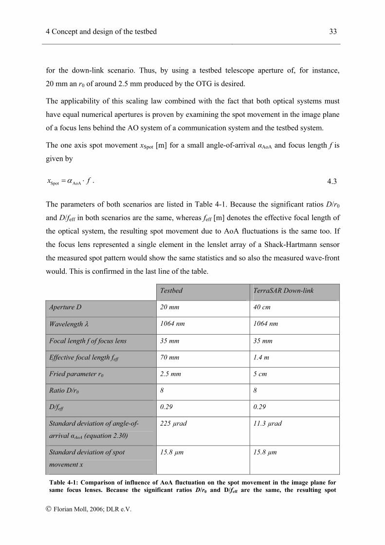
4 Concept and design of the testbed 33
© Florian Moll, 2006; DLR e.V.
for the down-link scenario. Thus, by using a testbed telescope aperture of, for instance,
20 mm an r0 of around 2.5 mm produced by the OTG is desired.
The applicability of this scaling law combined with the fact that both optical systems must
have equal numerical apertures is proven by examining the spot movement in the image plane
of a focus lens behind the AO system of a communication system and the testbed system.
The one axis spot movement xSpot [m] for a small angle-of-arrival αAoA and focus length f is
given by
Spot AoAx fα= ⋅ . 4.3
The parameters of both scenarios are listed in Table 4-1. Because the significant ratios D/r0
and D/feff in both scenarios are the same, whereas feff [m] denotes the effective focal length of
the optical system, the resulting spot movement due to AoA fluctuations is the same too. If
the focus lens represented a single element in the lenslet array of a Shack-Hartmann sensor
the measured spot pattern would show the same statistics and so also the measured wave-front
would. This is confirmed in the last line of the table.
Testbed TerraSAR Down-link
Aperture D 20 mm 40 cm
Wavelength λ 1064 nm 1064 nm
Focal length f of focus lens 35 mm 35 mm
Effective focal length feff 70 mm 1.4 m
Fried parameter r0 2.5 mm 5 cm
Ratio D/r0 8 8
D/feff 0.29 0.29
Standard deviation of angle-of-
arrival αAoA (equation 2.30)
225 µrad 11.3 µrad
Standard deviation of spot
movement x
15.8 µm 15.8 µm
Table 4-1: Comparison of influence of AoA fluctuation on the spot movement in the image plane for same focus lenses. Because the significant ratios D/r0 and D/feff are the same, the resulting spot
4 Concept and design of the testbed 34
© Florian Moll, 2006; DLR e.V.
movement due to AoA fluctuations is the same (last line).
Another scaling law includes the coherence outer scale and is given by
0
D const=Σ
. 4.4
This ratio is not as important as equation 4.2 but should be at least matched in the same order
of magnitude. For a LEO down-link scenario with 10° elevation, Σ0 is around 6 m. thus, the
ratio D/ Σ0 = 0.07. An aperture of 20 mm in the testbed results in the same ratio if Σ0 = 0.3 m.
4.2 Concept of the testbed
In the following the developed concept of the testbed shall be explained, which elements it
shall comprise and which elements are realized in the framework of this thesis. The testbed
contains three core components. These are the optical turbulence generator, the wave-front
sensor and the adaptive optics. The OTG reproduces wave-front distortions of a propagating
light beam which are sensed with the Shack-Hartmann device and corrected with the
deformable mirror and tip-tilt mirror. The OTG may be supplemented with a tilt generator that
adds tilt due to tracking errors. A couple of measurement devices are planned to be
implemented to characterize the effect of the optical turbulence on phase and intensity. A fast
focus camera (in the range of kHz) measures the short- and long-time exposure of a focus spot
to determine the Fried parameter and temporal behavior of the turbulence. A pupil camera
may capture the intensity distribution over the entrance pupil and a differential image motion
monitor measures r0. Furthermore a tracking sensor must be considered to create steering
signals for the tip-tilt mirror. Because the overall purpose of the testbed is to test techniques
for fiber coupling and small focus spot generation, a respective possibility in the testbed must
be taken care of. Further components are on the source side a variable optical attenuator
(VOA) to produce intensity fades, the transmitter telescope with fiber input and, on the
receiver side, the optical elements that form the receiver aperture, the beam
compression/expansion ratios, exit pupils for the measurement devices and path splitting.
The concept of the testbed is illustrated in Figure 4-1. In the main path of the sketch (bright
blue), the source is a fiber-coupled laser modulated with the communication signal. The
variable optical attenuator creates intensity fades directly behind the source. The source
collimator with the source fiber located in its focus produces a collimated beam that
4 Concept and design of the testbed 35
© Florian Moll, 2006; DLR e.V.
propagates through the OTG and tilt generator. In that way, the wave-front of the beam is
distorted dependent on the strength of the turbulence in the OTG and the angle-of-arrival is
modulated respectively. The receiver telescope collects the power and the exit pupil, formed
by the collimator element, is imaged on the tilt correcting element. All subsequent pupils
created by the optical system are conjugated to this one. The tip-tilt corrected beam is guided
onto a wave-front correction device which is placed in a further pupil. The optics image the
mirror plane on the wave-front sensor which measures the instantaneous wave-front that is
used to create the steering signals for the wave-front corrector. The first branch of Figure 4-1
behind the telescope (orange) contains two measurement devices whose purpose is to
characterize the grade of optical turbulence, the focus and the pupil camera. The second
branch behind the wave-front correction contains an optical port (that means another pupil)
for the DIMM to measure the r0 after the correction, the tracking-sensor system for creation of
input signals for the tip-tilt corrector, the fiber coupling system and an additional spare port.
The last port serves as docking port to the testbed where any kind of optical system can be
located, no matter if it needs a conjugate pupil or not.
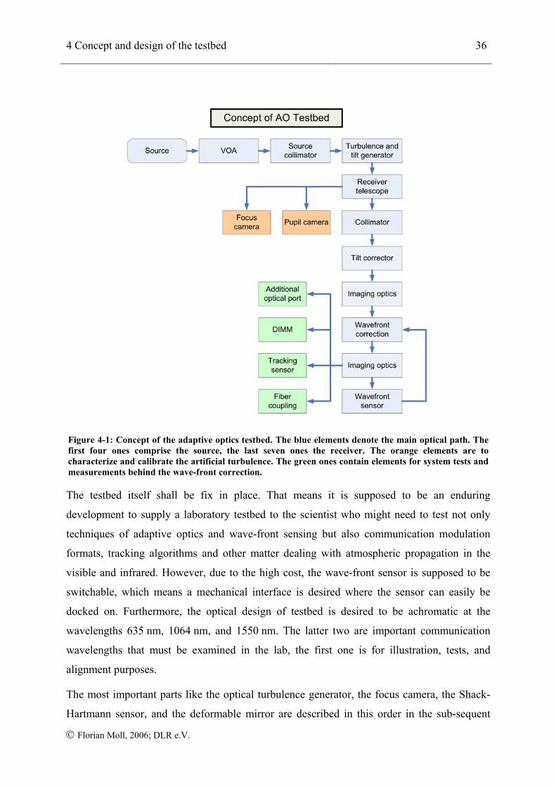
4 Concept and design of the testbed 36
© Florian Moll, 2006; DLR e.V.
Figure 4-1: Concept of the adaptive optics testbed. The blue elements denote the main optical path. The first four ones comprise the source, the last seven ones the receiver. The orange elements are to characterize and calibrate the artificial turbulence. The green ones contain elements for system tests and measurements behind the wave-front correction.
The testbed itself shall be fix in place. That means it is supposed to be an enduring
development to supply a laboratory testbed to the scientist who might need to test not only
techniques of adaptive optics and wave-front sensing but also communication modulation
formats, tracking algorithms and other matter dealing with atmospheric propagation in the
visible and infrared. However, due to the high cost, the wave-front sensor is supposed to be
switchable, which means a mechanical interface is desired where the sensor can easily be
docked on. Furthermore, the optical design of testbed is desired to be achromatic at the
wavelengths 635 nm, 1064 nm, and 1550 nm. The latter two are important communication
wavelengths that must be examined in the lab, the first one is for illustration, tests, and
alignment purposes.
The most important parts like the optical turbulence generator, the focus camera, the Shack-
Hartmann sensor, and the deformable mirror are described in this order in the sub-sequent
4 Concept and design of the testbed 37
© Florian Moll, 2006; DLR e.V.
chapters. A following sub-chapter is dedicated to the development, simulation and realization
of the optical design. The last sub-chapter contains a brief description of the remaining
hardware elements.
4.3 Optical turbulence generator
4.3.1 State of the art of optical turbulence generators
Ever since the atmosphere has been an impact on imaging performance and communications,
it has been an issue to generate artificial turbulence in the laboratory to simulate its behavior.
In the meantime, several techniques evolved, where three principles are most promising like
frozen phase screens, active, reconfigurable phase screens and turbulent fluid chambers
[Jol06]. No matter which one is chosen, phase variations with Kolmogorov statistics have to
be reproduced. The principle of frozen phase screens is to create an aberrated wave-front by
sending a plane wave through a transparent plate with non homogenous variation of index-of-
refraction or on an aberrated reflective surface. Both methods introduce an optical path
difference to the incident wave-front that is representative of a typical instantaneous turbulent
OPD following Kolmogorov statistics. Furthermore, several cascaded phase screens can be
applied in the propagation path to simulate several atmospheric layers of different turbulence
strength. With static phase screens, phase evolution is generated by movement of the screens,
e.g. rotation of a CD-like plate. These plates may be produced with various techniques like
polymer plate molding, glass polishing, microlithography, or near-index-matching. Dynamic
phase screens change their surface or index-of-refraction pattern directly. Applied devices are
spatial light modulators like liquid crystal devices or deformable mirrors. These two methods
have the advantage that the artificial turbulence is deterministic and thus, certain situations
may be repeated. Additionally, frozen turbulence behavior can be introduced by either
movement of the phase screen or respective control of the dynamic device. However, frozen
screens are able to simulate only one scenario, i.e. only a fix r0. Dynamic screens do not suffer
from this problem but are slow, in the case of using liquid crystal SLMs (Spatial Light
Modulators), or cannot produce high spatial frequencies, in the case of deformable mirrors.
Additionally, both methods have limited stroke which means an upper limit of OPD and thus,
lowers turbulence dynamics. Turbulent fluid based OTGs are somewhat different from the
other ones. Here, the idea is to create real, physical turbulence in a confined space by mixing
of two flows of air, water or any other fluid at different temperatures. Dynamical turbulence is
4 Concept and design of the testbed 38
© Florian Moll, 2006; DLR e.V.
created by the forced mixing of the flows in the turbulent chamber, and, since the flows bear
different temperatures, a turbulent field of refractive index is created. Suggested fluids are
water and air. A big advantage of this method is its natural behavior which makes sure the
realistic behavior with high turbulence dynamic. Also, if calibrated, certain scenarios can be
statistically reproduced. But high temperatures, up to 473 K, have to be handled, which is
maybe not possible in every optics lab. A more detailed discussion of the different methods
and fabrication of phase screens is given in [Jol06]. Moreover, the issue of cost determines the
choice.
Although, the method of rotating static phase screens seems to be most comfortable and clean,
it comes out to be very expensive. In [Kol04] three phase screens are cascaded for simulations
with the MAPS (Multi Atmospheric Phase screens and Stars) turbulence simulator at the
European Southern Observatory (ESO). By rearranging the screens, the drawback of being
limited to one scenario is partly eliminated. The same screens are applied at the University of
Galway. The essential reason for not choosing these phase screens is the cost of at least
5 000 € per element which exceeds the budget for the testbed. A cheap alternative may be the
use of simple shower glass as applied in [Wei74] to simulate turbulence in speckle
interferometry. However, the realism here is questionable. Another approach is the use of
spatial light modulators as done in [Bur08] but these are slow and expansive, too. Research
shows that most laboratories apply hot air turbulence chambers, probably due to their realistic
performance and low cost. Some relevant publications shall be mentioned in this context that
influence the choice, like the work of Majumdar and Gamo [Gam78] [Maj82] [Maj98], Fuchs
[Fuc96], Abtahi [Abt06], and Keskin [Kes06]. Thus, due to realism, low cost and proven
experience the method of hot-air optical turbulence generators is chosen whose realization is
explained in the subsequent chapter.
4.3.2 Hot-air optical turbulence generator
The construction of the OTG for the AO testbed is mainly inspired by the suggestions of
[Jol06] and [Kes06] who developed their devices for the ESO. The concept is a guided
confrontation of a cold and hot air flow in a mixing chamber. The temperature difference
Tdiff [K] of the flows then determines the strength of turbulence. This method has been proven
to produce realistic turbulence by measuring the angle-of-arrival spectral power density and
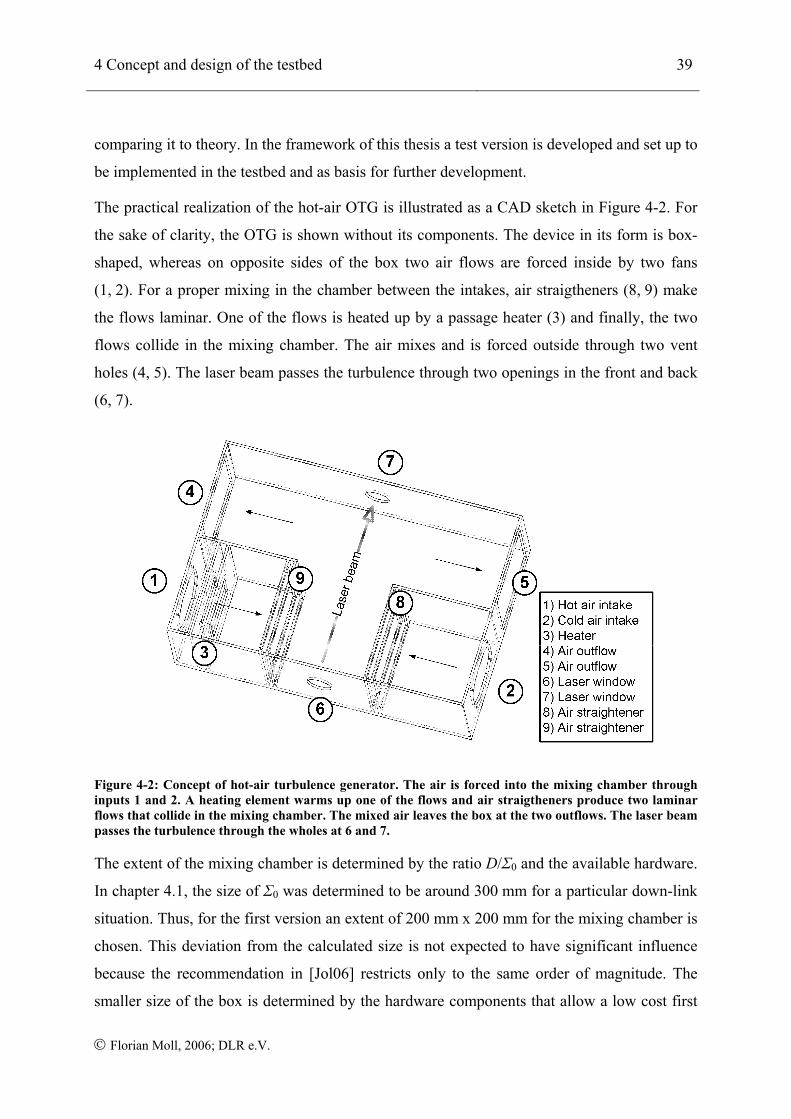
4 Concept and design of the testbed 39
© Florian Moll, 2006; DLR e.V.
comparing it to theory. In the framework of this thesis a test version is developed and set up to
be implemented in the testbed and as basis for further development.
The practical realization of the hot-air OTG is illustrated as a CAD sketch in Figure 4-2. For
the sake of clarity, the OTG is shown without its components. The device in its form is box-
shaped, whereas on opposite sides of the box two air flows are forced inside by two fans
(1, 2). For a proper mixing in the chamber between the intakes, air straigtheners (8, 9) make
the flows laminar. One of the flows is heated up by a passage heater (3) and finally, the two
flows collide in the mixing chamber. The air mixes and is forced outside through two vent
holes (4, 5). The laser beam passes the turbulence through two openings in the front and back
(6, 7).
Figure 4-2: Concept of hot-air turbulence generator. The air is forced into the mixing chamber through inputs 1 and 2. A heating element warms up one of the flows and air straigtheners produce two laminar flows that collide in the mixing chamber. The mixed air leaves the box at the two outflows. The laser beam passes the turbulence through the wholes at 6 and 7.
The extent of the mixing chamber is determined by the ratio D/Σ0 and the available hardware.
In chapter 4.1, the size of Σ0 was determined to be around 300 mm for a particular down-link
situation. Thus, for the first version an extent of 200 mm x 200 mm for the mixing chamber is
chosen. This deviation from the calculated size is not expected to have significant influence
because the recommendation in [Jol06] restricts only to the same order of magnitude. The
smaller size of the box is determined by the hardware components that allow a low cost first
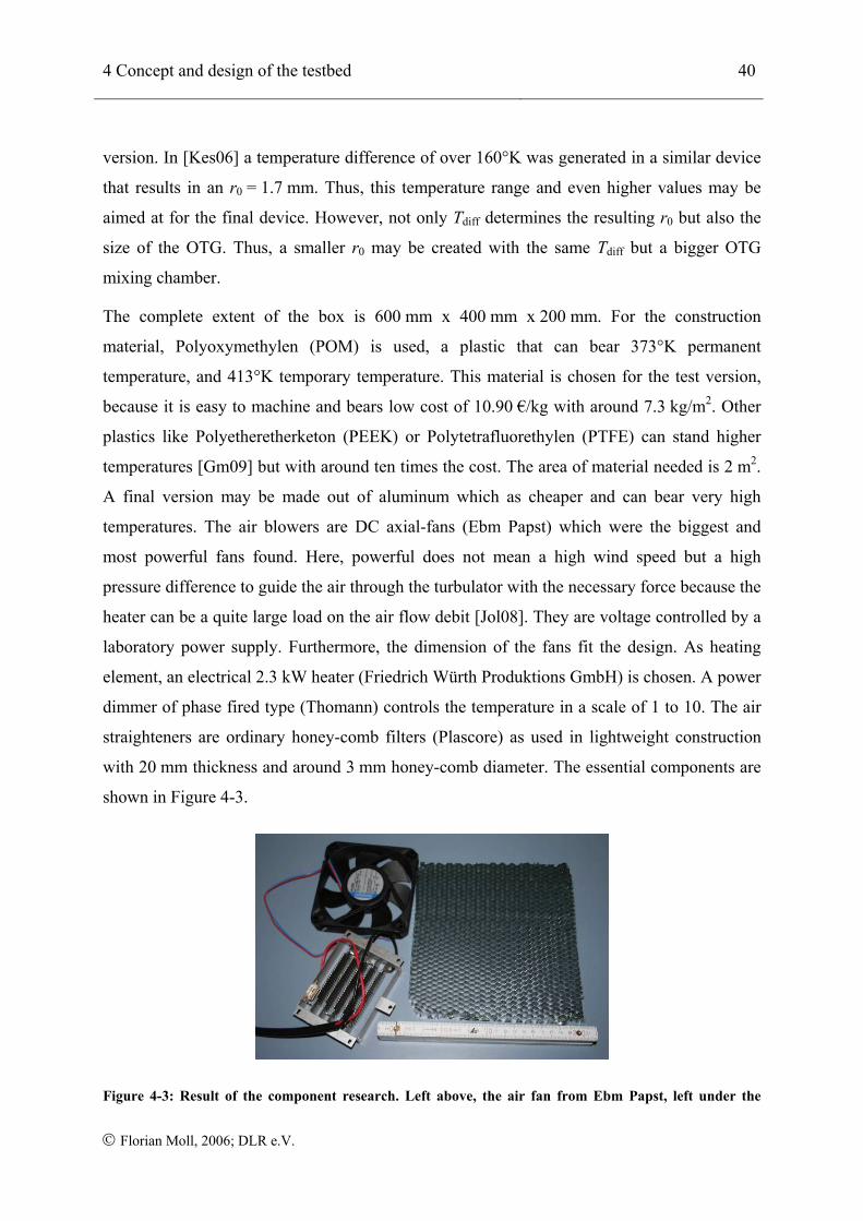
4 Concept and design of the testbed 40
© Florian Moll, 2006; DLR e.V.
version. In [Kes06] a temperature difference of over 160°K was generated in a similar device
that results in an r0 = 1.7 mm. Thus, this temperature range and even higher values may be
aimed at for the final device. However, not only Tdiff determines the resulting r0 but also the
size of the OTG. Thus, a smaller r0 may be created with the same Tdiff but a bigger OTG
mixing chamber.
The complete extent of the box is 600 mm x 400 mm x 200 mm. For the construction
material, Polyoxymethylen (POM) is used, a plastic that can bear 373°K permanent
temperature, and 413°K temporary temperature. This material is chosen for the test version,
because it is easy to machine and bears low cost of 10.90 €/kg with around 7.3 kg/m2. Other
plastics like Polyetheretherketon (PEEK) or Polytetrafluorethylen (PTFE) can stand higher
temperatures [Gm09] but with around ten times the cost. The area of material needed is 2 m2.
A final version may be made out of aluminum which as cheaper and can bear very high
temperatures. The air blowers are DC axial-fans (Ebm Papst) which were the biggest and
most powerful fans found. Here, powerful does not mean a high wind speed but a high
pressure difference to guide the air through the turbulator with the necessary force because the
heater can be a quite large load on the air flow debit [Jol08]. They are voltage controlled by a
laboratory power supply. Furthermore, the dimension of the fans fit the design. As heating
element, an electrical 2.3 kW heater (Friedrich Würth Produktions GmbH) is chosen. A power
dimmer of phase fired type (Thomann) controls the temperature in a scale of 1 to 10. The air
straighteners are ordinary honey-comb filters (Plascore) as used in lightweight construction
with 20 mm thickness and around 3 mm honey-comb diameter. The essential components are
shown in Figure 4-3.
Figure 4-3: Result of the component research. Left above, the air fan from Ebm Papst, left under the
4 Concept and design of the testbed 41
© Florian Moll, 2006; DLR e.V.
2.3 kw electrical heating element from Friedrich Würth Produktions GmbH, and the honey-comb filter from Plascore.
The assembled test version is shown in Figure 4-4. The Voltcraft thermometers measure the
temperature of the two air flows. Also, an amendment to the initial design in Figure 4-2 is
visible. It is a small box added on the side of the hot-air intake which is necessary to enlarge
the distance between the air fan and heater. In the initial design, this distance was too small
and thus, the fan heated up after a while and failed.
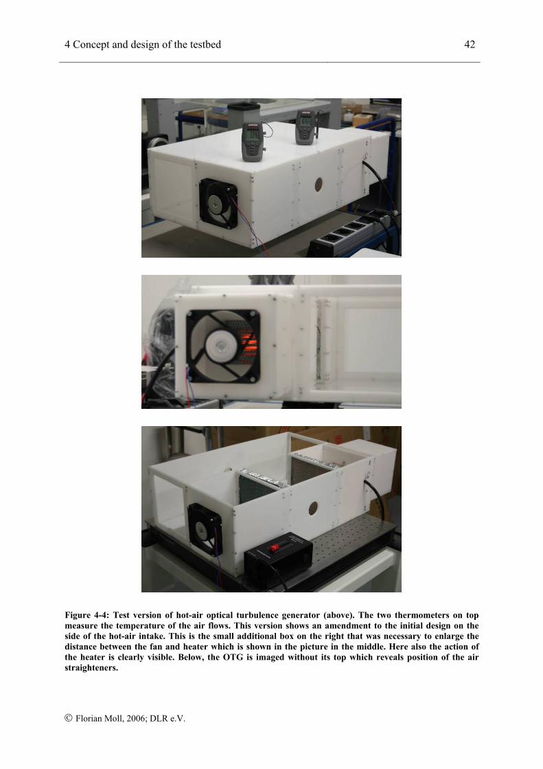
4 Concept and design of the testbed 42
© Florian Moll, 2006; DLR e.V.
Figure 4-4: Test version of hot-air optical turbulence generator (above). The two thermometers on top measure the temperature of the air flows. This version shows an amendment to the initial design on the side of the hot-air intake. This is the small additional box on the right that was necessary to enlarge the distance between the fan and heater which is shown in the picture in the middle. Here also the action of the heater is clearly visible. Below, the OTG is imaged without its top which reveals position of the air straighteners.
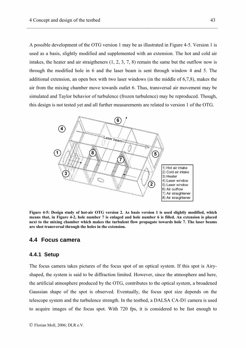
4 Concept and design of the testbed 43
© Florian Moll, 2006; DLR e.V.
A possible development of the OTG version 1 may be as illustrated in Figure 4-5. Version 1 is
used as a basis, slightly modified and supplemented with an extension. The hot and cold air
intakes, the heater and air straigtheners (1, 2, 3, 7, 8) remain the same but the outflow now is
through the modified hole in 6 and the laser beam is sent through window 4 and 5. The
additional extension, an open box with two laser windows (in the middle of 6,7,8), makes the
air from the mixing chamber move towards outlet 6. Thus, transversal air movement may be
simulated and Taylor behavior of turbulence (frozen turbulence) may be reproduced. Though,
this design is not tested yet and all further measurements are related to version 1 of the OTG.
Figure 4-5: Design study of hot-air OTG version 2. As basis version 1 is used slightly modified, which means that, in Figure 4-2, hole number 7 is enlaged and hole number 6 is filled. An extension is placed next to the mixing chamber which makes the turbulent flow propagate towards hole 7. The laser beams are shot transversal through the holes in the extension.
4.4 Focus camera
4.4.1 Setup
The focus camera takes pictures of the focus spot of an optical system. If this spot is Airy-
shaped, the system is said to be diffraction limited. However, since the atmosphere and here,
the artificial atmosphere produced by the OTG, contributes to the optical system, a broadened
Gaussian shape of the spot is observed. Eventually, the focus spot size depends on the
telescope system and the turbulence strength. In the testbed, a DALSA CA-D1 camera is used
to acquire images of the focus spot. With 720 fps, it is considered to be fast enough to
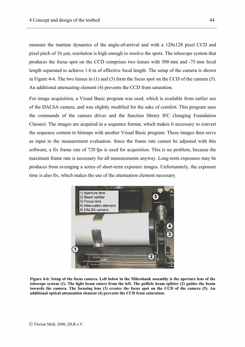
4 Concept and design of the testbed 44
© Florian Moll, 2006; DLR e.V.
measure the runtime dynamics of the angle-of-arrival and with a 128x128 pixel CCD and
pixel pitch of 16 µm, resolution is high enough to resolve the spots. The telescope system that
produces the focus spot on the CCD comprises two lenses with 500 mm and -75 mm focal
length separated to achieve 1.6 m of effective focal length. The setup of the camera is shown
in Figure 4-6. The two lenses in (1) and (3) form the focus spot on the CCD of the camera (5).
An additional attenuating element (4) prevents the CCD from saturation.
For image acquisition, a Visual Basic program was used, which is available from earlier use
of the DALSA camera, and was slightly modified for the sake of comfort. This program uses
the commands of the camera driver and the function library IFC (Imaging Foundation
Classes). The images are acquired in a sequence format, which makes it necessary to convert
the sequence content to bitmaps with another Visual Basic program. These images then serve
as input to the measurement evaluation. Since the frame rate cannot be adjusted with this
software, a fix frame rate of 720 fps is used for acquisition. This is no problem, because the
maximum frame rate is necessary for all measurements anyway. Long-term exposures may be
produces from averaging a series of short-term exposure images. Unfortunately, the exposure
time is also fix, which makes the use of the attenuation element necessary.
Figure 4-6: Setup of the focus camera. Left below in the Mikrobank assembly is the aperture lens of the telescope system (1). The light beam enters from the left. The pellicle beam splitter (2) guides the beam towards the camera. The focusing lens (3) creates the focus spot on the CCD of the camera (5). An additional optical attenuation element (4) prevents the CCD from saturation.
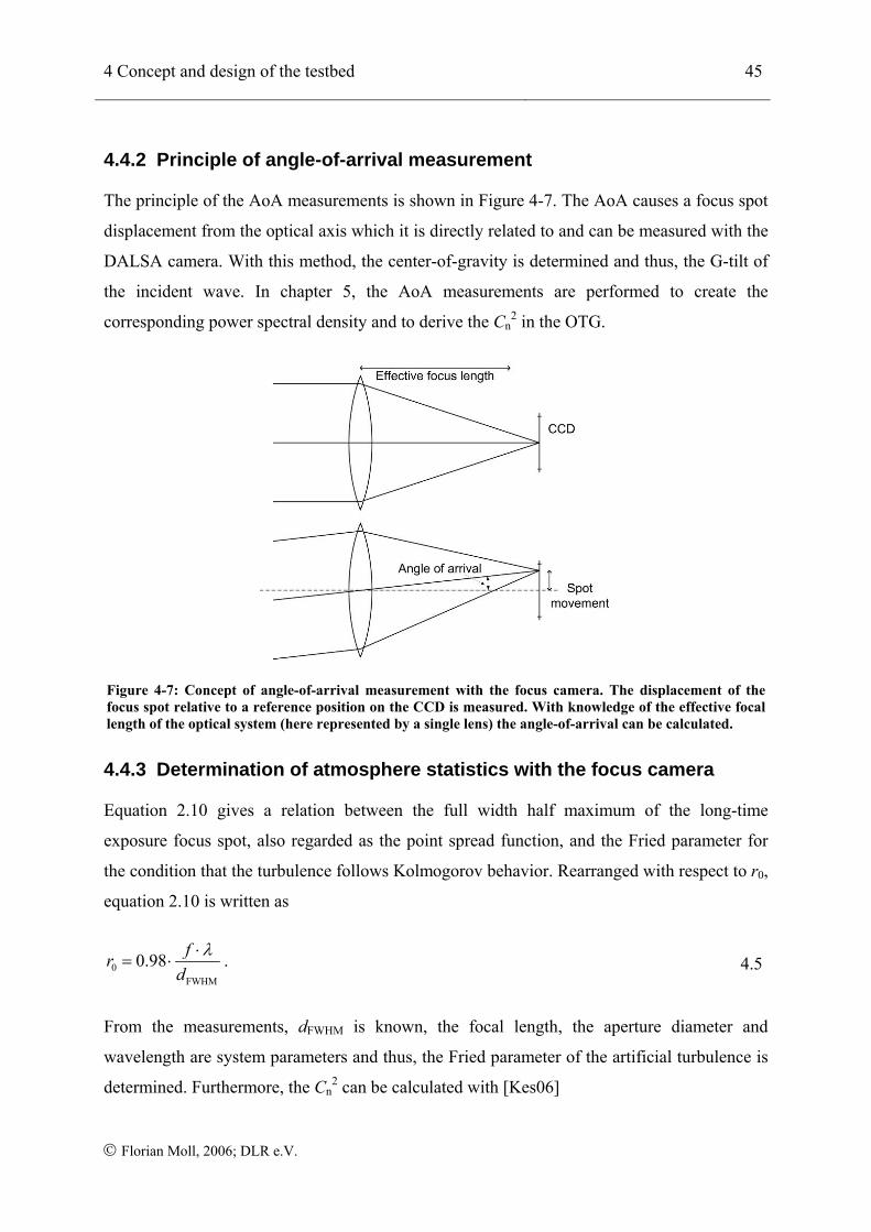
4 Concept and design of the testbed 45
© Florian Moll, 2006; DLR e.V.
4.4.2 Principle of angle-of-arrival measurement
The principle of the AoA measurements is shown in Figure 4-7. The AoA causes a focus spot
displacement from the optical axis which it is directly related to and can be measured with the
DALSA camera. With this method, the center-of-gravity is determined and thus, the G-tilt of
the incident wave. In chapter 5, the AoA measurements are performed to create the
corresponding power spectral density and to derive the Cn2 in the OTG.
Figure 4-7: Concept of angle-of-arrival measurement with the focus camera. The displacement of the focus spot relative to a reference position on the CCD is measured. With knowledge of the effective focal length of the optical system (here represented by a single lens) the angle-of-arrival can be calculated.
4.4.3 Determination of atmosphere statistics with the focus camera
Equation 2.10 gives a relation between the full width half maximum of the long-time
exposure focus spot, also regarded as the point spread function, and the Fried parameter for
the condition that the turbulence follows Kolmogorov behavior. Rearranged with respect to r0,
equation 2.10 is written as
0FWHM
0.98 frd
λ⋅= ⋅ . 4.5
From the measurements, dFWHM is known, the focal length, the aperture diameter and
wavelength are system parameters and thus, the Fried parameter of the artificial turbulence is
determined. Furthermore, the Cn2 can be calculated with [Kes06]
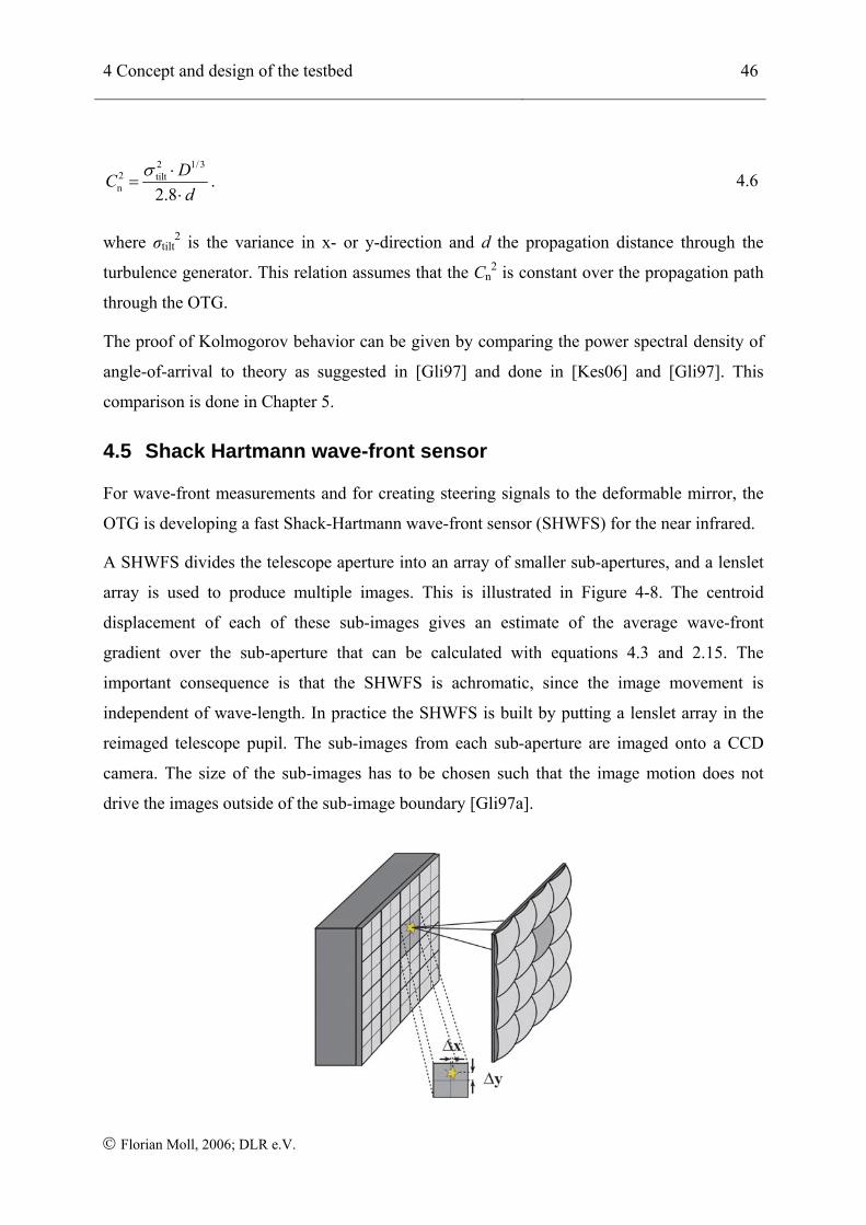
4 Concept and design of the testbed 46
© Florian Moll, 2006; DLR e.V.
2 1/32 tiltn 2.8
DCd
σ ⋅=
⋅. 4.6
where σtilt2 is the variance in x- or y-direction and d the propagation distance through the
turbulence generator. This relation assumes that the Cn2 is constant over the propagation path
through the OTG.
The proof of Kolmogorov behavior can be given by comparing the power spectral density of
angle-of-arrival to theory as suggested in [Gli97] and done in [Kes06] and [Gli97]. This
comparison is done in Chapter 5.
4.5 Shack Hartmann wave-front sensor
For wave-front measurements and for creating steering signals to the deformable mirror, the
OTG is developing a fast Shack-Hartmann wave-front sensor (SHWFS) for the near infrared.
A SHWFS divides the telescope aperture into an array of smaller sub-apertures, and a lenslet
array is used to produce multiple images. This is illustrated in Figure 4-8. The centroid
displacement of each of these sub-images gives an estimate of the average wave-front
gradient over the sub-aperture that can be calculated with equations 4.3 and 2.15. The
important consequence is that the SHWFS is achromatic, since the image movement is
independent of wave-length. In practice the SHWFS is built by putting a lenslet array in the
reimaged telescope pupil. The sub-images from each sub-aperture are imaged onto a CCD
camera. The size of the sub-images has to be chosen such that the image motion does not
drive the images outside of the sub-image boundary [Gli97a].
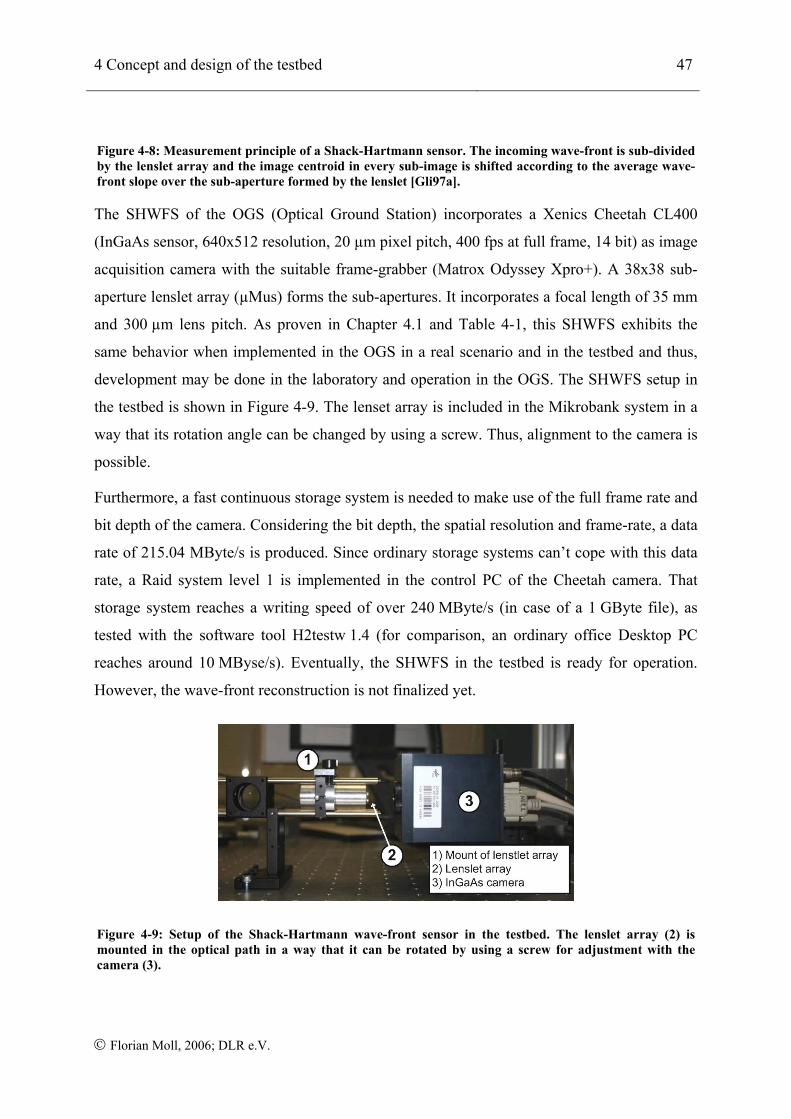
4 Concept and design of the testbed 47
© Florian Moll, 2006; DLR e.V.
Figure 4-8: Measurement principle of a Shack-Hartmann sensor. The incoming wave-front is sub-divided by the lenslet array and the image centroid in every sub-image is shifted according to the average wave-front slope over the sub-aperture formed by the lenslet [Gli97a].
The SHWFS of the OGS (Optical Ground Station) incorporates a Xenics Cheetah CL400
(InGaAs sensor, 640x512 resolution, 20 µm pixel pitch, 400 fps at full frame, 14 bit) as image
acquisition camera with the suitable frame-grabber (Matrox Odyssey Xpro+). A 38x38 sub-
aperture lenslet array (µMus) forms the sub-apertures. It incorporates a focal length of 35 mm
and 300 µm lens pitch. As proven in Chapter 4.1 and Table 4-1, this SHWFS exhibits the
same behavior when implemented in the OGS in a real scenario and in the testbed and thus,
development may be done in the laboratory and operation in the OGS. The SHWFS setup in
the testbed is shown in Figure 4-9. The lenset array is included in the Mikrobank system in a
way that its rotation angle can be changed by using a screw. Thus, alignment to the camera is
possible.
Furthermore, a fast continuous storage system is needed to make use of the full frame rate and
bit depth of the camera. Considering the bit depth, the spatial resolution and frame-rate, a data
rate of 215.04 MByte/s is produced. Since ordinary storage systems can’t cope with this data
rate, a Raid system level 1 is implemented in the control PC of the Cheetah camera. That
storage system reaches a writing speed of over 240 MByte/s (in case of a 1 GByte file), as
tested with the software tool H2testw 1.4 (for comparison, an ordinary office Desktop PC
reaches around 10 MByse/s). Eventually, the SHWFS in the testbed is ready for operation.
However, the wave-front reconstruction is not finalized yet.
Figure 4-9: Setup of the Shack-Hartmann wave-front sensor in the testbed. The lenslet array (2) is mounted in the optical path in a way that it can be rotated by using a screw for adjustment with the camera (3).
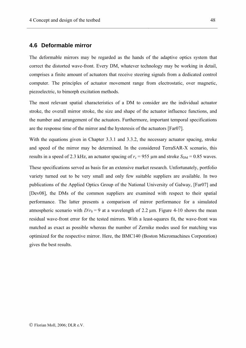
4 Concept and design of the testbed 48
© Florian Moll, 2006; DLR e.V.
4.6 Deformable mirror
The deformable mirrors may be regarded as the hands of the adaptive optics system that
correct the distorted wave-front. Every DM, whatever technology may be working in detail,
comprises a finite amount of actuators that receive steering signals from a dedicated control
computer. The principles of actuator movement range from electrostatic, over magnetic,
piezoelectric, to bimorph excitation methods.
The most relevant spatial characteristics of a DM to consider are the individual actuator
stroke, the overall mirror stroke, the size and shape of the actuator influence functions, and
the number and arrangement of the actuators. Furthermore, important temporal specifications
are the response time of the mirror and the hysteresis of the actuators [Far07].
With the equations given in Chapter 3.3.1 and 3.3.2, the necessary actuator spacing, stroke
and speed of the mirror may be determined. In the considered TerraSAR-X scenario, this
results in a speed of 2.3 kHz, an actuator spacing of rc = 955 µm and stroke SDM = 0.85 waves.
These specifications served as basis for an extensive market research. Unfortunately, portfolio
variety turned out to be very small and only few suitable suppliers are available. In two
publications of the Applied Optics Group of the National University of Galway, [Far07] and
[Dev08], the DMs of the common suppliers are examined with respect to their spatial
performance. The latter presents a comparison of mirror performance for a simulated
atmospheric scenario with D/r0 = 9 at a wavelength of 2.2 µm. Figure 4-10 shows the mean
residual wave-front error for the tested mirrors. With a least-squares fit, the wave-front was
matched as exact as possible whereas the number of Zernike modes used for matching was
optimized for the respective mirror. Here, the BMC140 (Boston Micromachines Corporation)
gives the best results.
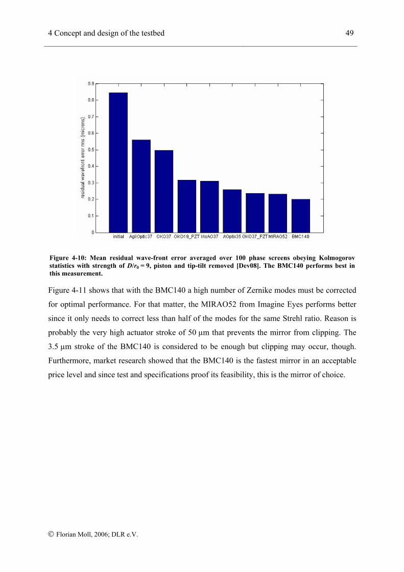
4 Concept and design of the testbed 49
© Florian Moll, 2006; DLR e.V.
Figure 4-10: Mean residual wave-front error averaged over 100 phase screens obeying Kolmogorov statistics with strength of D/r0 = 9, piston and tip-tilt removed [Dev08]. The BMC140 performs best in this measurement.
Figure 4-11 shows that with the BMC140 a high number of Zernike modes must be corrected
for optimal performance. For that matter, the MIRAO52 from Imagine Eyes performs better
since it only needs to correct less than half of the modes for the same Strehl ratio. Reason is
probably the very high actuator stroke of 50 µm that prevents the mirror from clipping. The
3.5 µm stroke of the BMC140 is considered to be enough but clipping may occur, though.
Furthermore, market research showed that the BMC140 is the fastest mirror in an acceptable
price level and since test and specifications proof its feasibility, this is the mirror of choice.
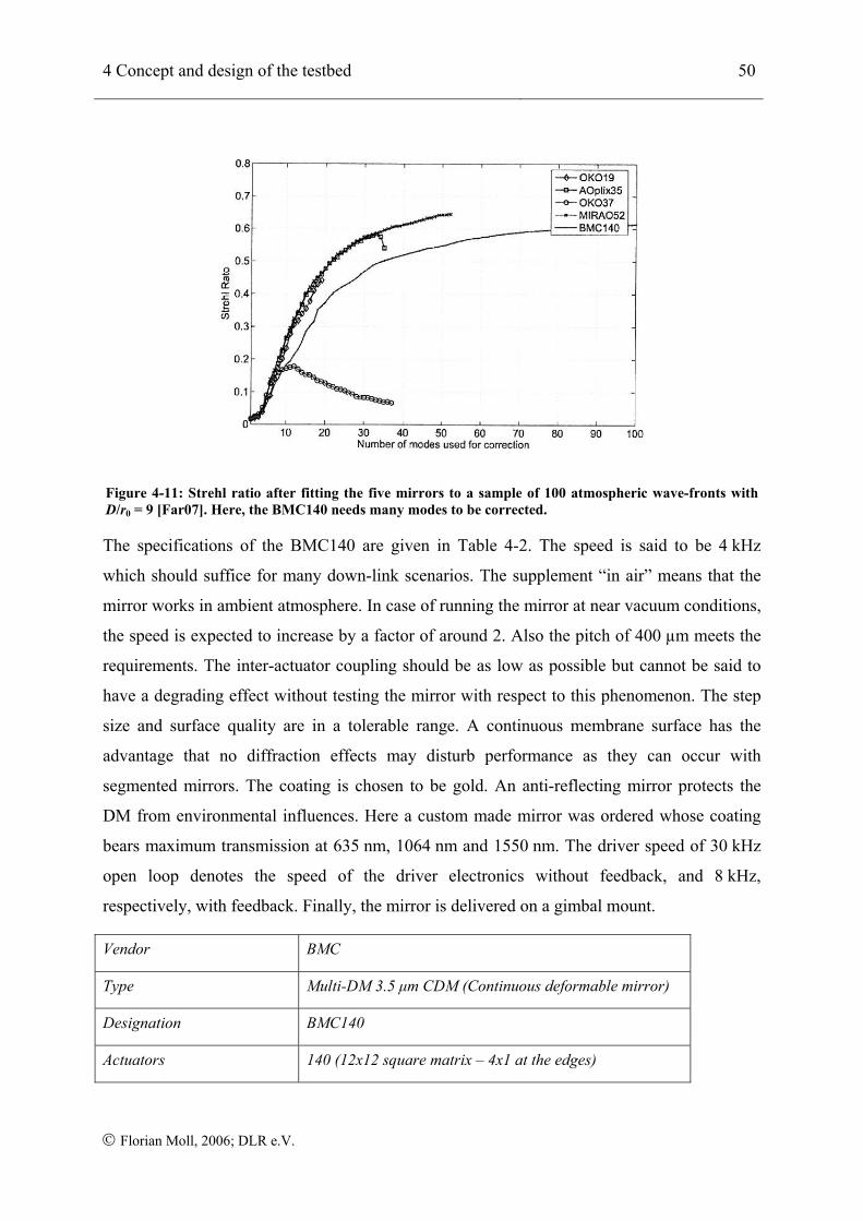
4 Concept and design of the testbed 50
© Florian Moll, 2006; DLR e.V.
Figure 4-11: Strehl ratio after fitting the five mirrors to a sample of 100 atmospheric wave-fronts with D/r0 = 9 [Far07]. Here, the BMC140 needs many modes to be corrected.
The specifications of the BMC140 are given in Table 4-2. The speed is said to be 4 kHz
which should suffice for many down-link scenarios. The supplement “in air” means that the
mirror works in ambient atmosphere. In case of running the mirror at near vacuum conditions,
the speed is expected to increase by a factor of around 2. Also the pitch of 400 µm meets the
requirements. The inter-actuator coupling should be as low as possible but cannot be said to
have a degrading effect without testing the mirror with respect to this phenomenon. The step
size and surface quality are in a tolerable range. A continuous membrane surface has the
advantage that no diffraction effects may disturb performance as they can occur with
segmented mirrors. The coating is chosen to be gold. An anti-reflecting mirror protects the
DM from environmental influences. Here a custom made mirror was ordered whose coating
bears maximum transmission at 635 nm, 1064 nm and 1550 nm. The driver speed of 30 kHz
open loop denotes the speed of the driver electronics without feedback, and 8 kHz,
respectively, with feedback. Finally, the mirror is delivered on a gimbal mount.
Vendor BMC
Type Multi-DM 3.5 µm CDM (Continuous deformable mirror)
Designation BMC140
Actuators 140 (12x12 square matrix – 4x1 at the edges)
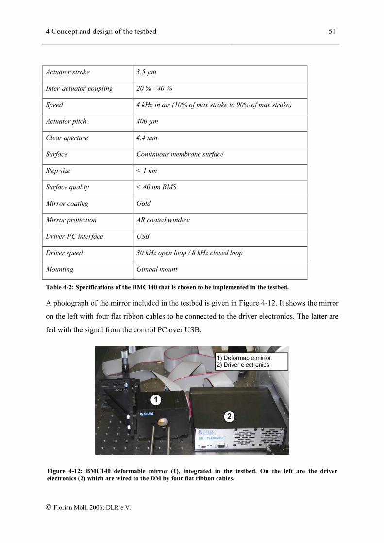
4 Concept and design of the testbed 51
© Florian Moll, 2006; DLR e.V.
Actuator stroke 3.5 µm
Inter-actuator coupling 20 % - 40 %
Speed 4 kHz in air (10% of max stroke to 90% of max stroke)
Actuator pitch 400 µm
Clear aperture 4.4 mm
Surface Continuous membrane surface
Step size < 1 nm
Surface quality < 40 nm RMS
Mirror coating Gold
Mirror protection AR coated window
Driver-PC interface USB
Driver speed 30 kHz open loop / 8 kHz closed loop
Mounting Gimbal mount
Table 4-2: Specifications of the BMC140 that is chosen to be implemented in the testbed.
A photograph of the mirror included in the testbed is given in Figure 4-12. It shows the mirror
on the left with four flat ribbon cables to be connected to the driver electronics. The latter are
fed with the signal from the control PC over USB.
Figure 4-12: BMC140 deformable mirror (1), integrated in the testbed. On the left are the driver electronics (2) which are wired to the DM by four flat ribbon cables.
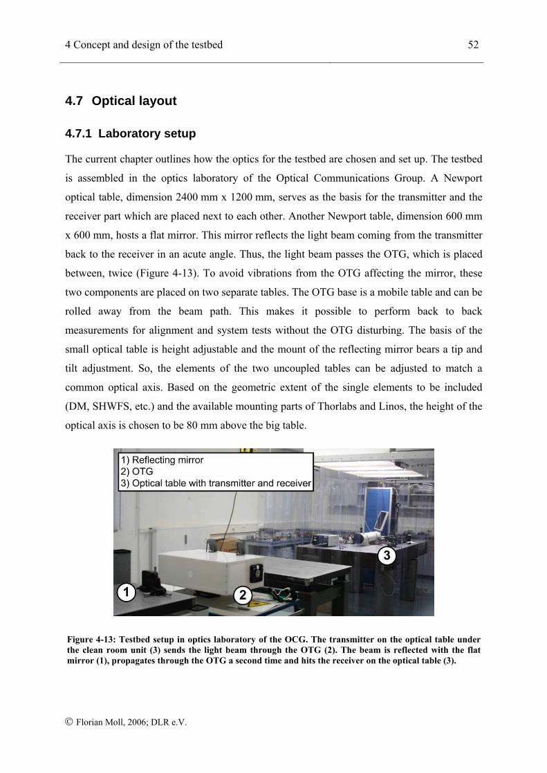
4 Concept and design of the testbed 52
© Florian Moll, 2006; DLR e.V.
4.7 Optical layout
4.7.1 Laboratory setup
The current chapter outlines how the optics for the testbed are chosen and set up. The testbed
is assembled in the optics laboratory of the Optical Communications Group. A Newport
optical table, dimension 2400 mm x 1200 mm, serves as the basis for the transmitter and the
receiver part which are placed next to each other. Another Newport table, dimension 600 mm
x 600 mm, hosts a flat mirror. This mirror reflects the light beam coming from the transmitter
back to the receiver in an acute angle. Thus, the light beam passes the OTG, which is placed
between, twice (Figure 4-13). To avoid vibrations from the OTG affecting the mirror, these
two components are placed on two separate tables. The OTG base is a mobile table and can be
rolled away from the beam path. This makes it possible to perform back to back
measurements for alignment and system tests without the OTG disturbing. The basis of the
small optical table is height adjustable and the mount of the reflecting mirror bears a tip and
tilt adjustment. So, the elements of the two uncoupled tables can be adjusted to match a
common optical axis. Based on the geometric extent of the single elements to be included
(DM, SHWFS, etc.) and the available mounting parts of Thorlabs and Linos, the height of the
optical axis is chosen to be 80 mm above the big table.
Figure 4-13: Testbed setup in optics laboratory of the OCG. The transmitter on the optical table under the clean room unit (3) sends the light beam through the OTG (2). The beam is reflected with the flat mirror (1), propagates through the OTG a second time and hits the receiver on the optical table (3).
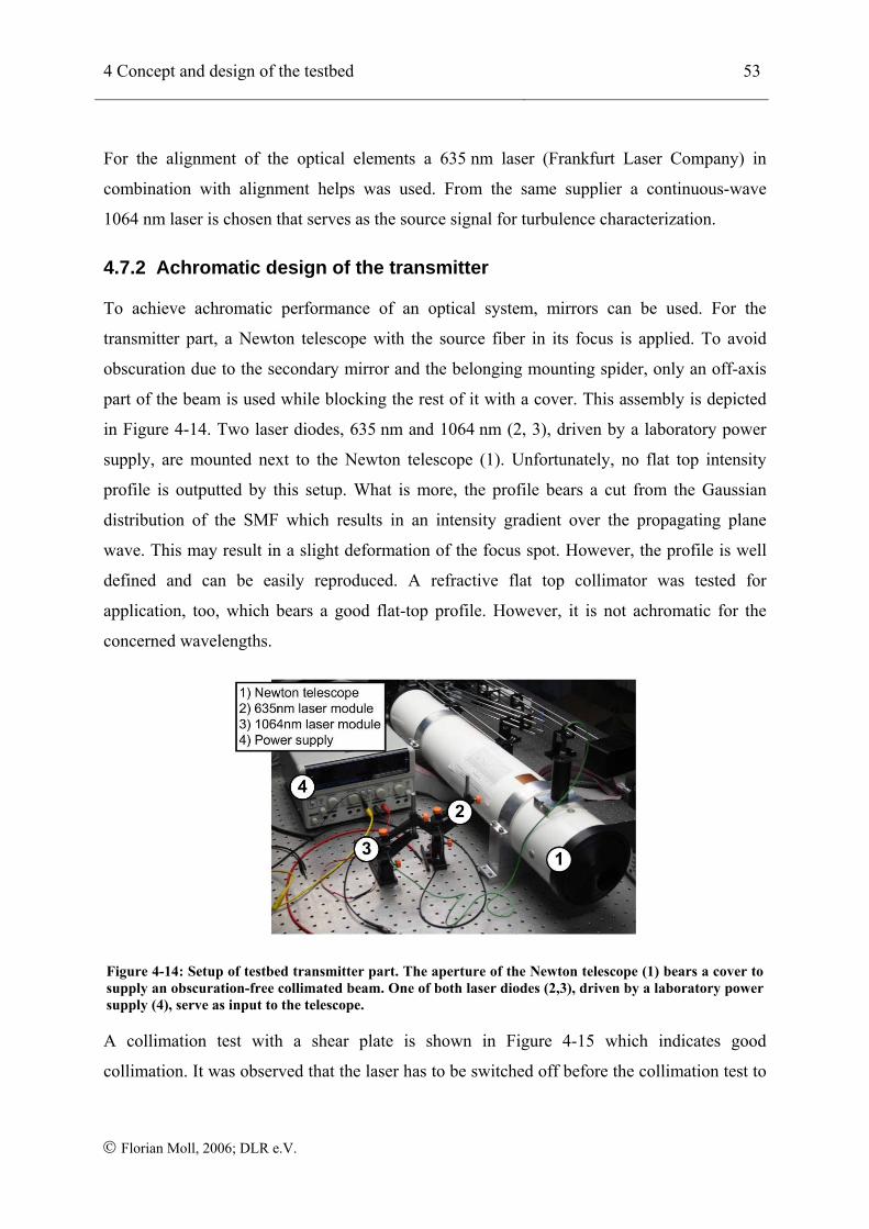
4 Concept and design of the testbed 53
© Florian Moll, 2006; DLR e.V.
For the alignment of the optical elements a 635 nm laser (Frankfurt Laser Company) in
combination with alignment helps was used. From the same supplier a continuous-wave
1064 nm laser is chosen that serves as the source signal for turbulence characterization.
4.7.2 Achromatic design of the transmitter
To achieve achromatic performance of an optical system, mirrors can be used. For the
transmitter part, a Newton telescope with the source fiber in its focus is applied. To avoid
obscuration due to the secondary mirror and the belonging mounting spider, only an off-axis
part of the beam is used while blocking the rest of it with a cover. This assembly is depicted
in Figure 4-14. Two laser diodes, 635 nm and 1064 nm (2, 3), driven by a laboratory power
supply, are mounted next to the Newton telescope (1). Unfortunately, no flat top intensity
profile is outputted by this setup. What is more, the profile bears a cut from the Gaussian
distribution of the SMF which results in an intensity gradient over the propagating plane
wave. This may result in a slight deformation of the focus spot. However, the profile is well
defined and can be easily reproduced. A refractive flat top collimator was tested for
application, too, which bears a good flat-top profile. However, it is not achromatic for the
concerned wavelengths.
Figure 4-14: Setup of testbed transmitter part. The aperture of the Newton telescope (1) bears a cover to supply an obscuration-free collimated beam. One of both laser diodes (2,3), driven by a laboratory power supply (4), serve as input to the telescope.
A collimation test with a shear plate is shown in Figure 4-15 which indicates good
collimation. It was observed that the laser has to be switched off before the collimation test to
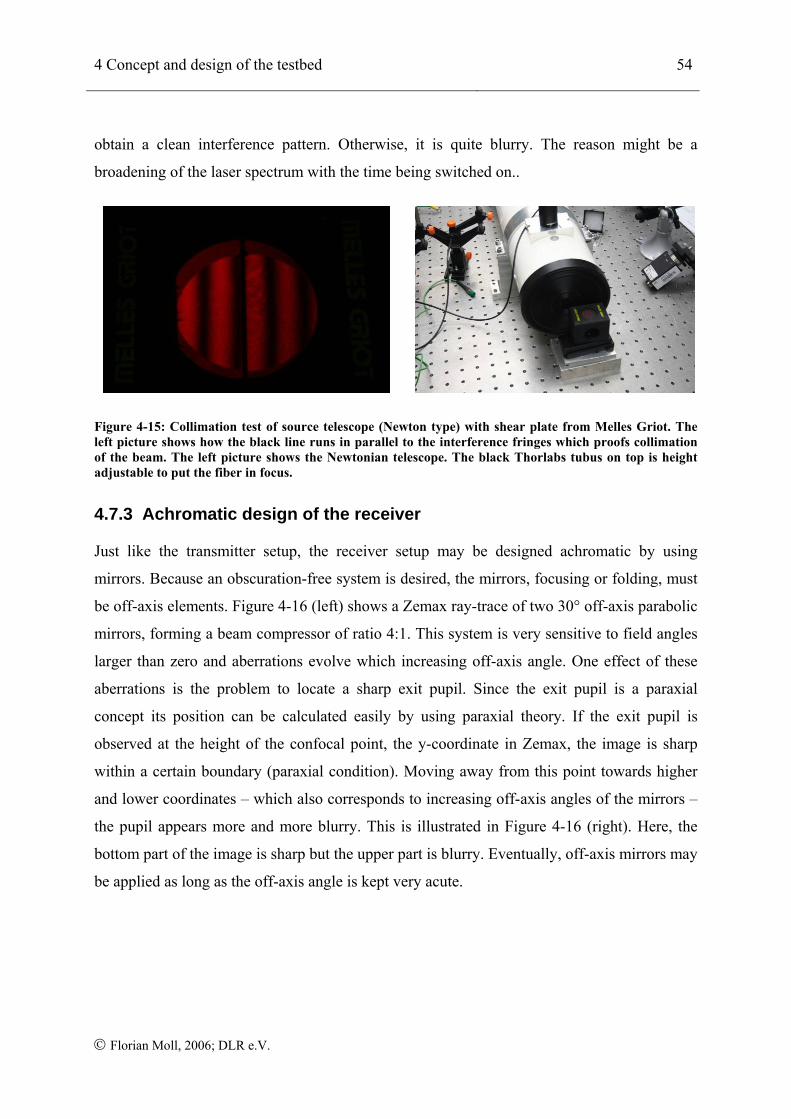
4 Concept and design of the testbed 54
© Florian Moll, 2006; DLR e.V.
obtain a clean interference pattern. Otherwise, it is quite blurry. The reason might be a
broadening of the laser spectrum with the time being switched on..
Figure 4-15: Collimation test of source telescope (Newton type) with shear plate from Melles Griot. The left picture shows how the black line runs in parallel to the interference fringes which proofs collimation of the beam. The left picture shows the Newtonian telescope. The black Thorlabs tubus on top is height adjustable to put the fiber in focus.
4.7.3 Achromatic design of the receiver
Just like the transmitter setup, the receiver setup may be designed achromatic by using
mirrors. Because an obscuration-free system is desired, the mirrors, focusing or folding, must
be off-axis elements. Figure 4-16 (left) shows a Zemax ray-trace of two 30° off-axis parabolic
mirrors, forming a beam compressor of ratio 4:1. This system is very sensitive to field angles
larger than zero and aberrations evolve which increasing off-axis angle. One effect of these
aberrations is the problem to locate a sharp exit pupil. Since the exit pupil is a paraxial
concept its position can be calculated easily by using paraxial theory. If the exit pupil is
observed at the height of the confocal point, the y-coordinate in Zemax, the image is sharp
within a certain boundary (paraxial condition). Moving away from this point towards higher
and lower coordinates – which also corresponds to increasing off-axis angles of the mirrors –
the pupil appears more and more blurry. This is illustrated in Figure 4-16 (right). Here, the
bottom part of the image is sharp but the upper part is blurry. Eventually, off-axis mirrors may
be applied as long as the off-axis angle is kept very acute.
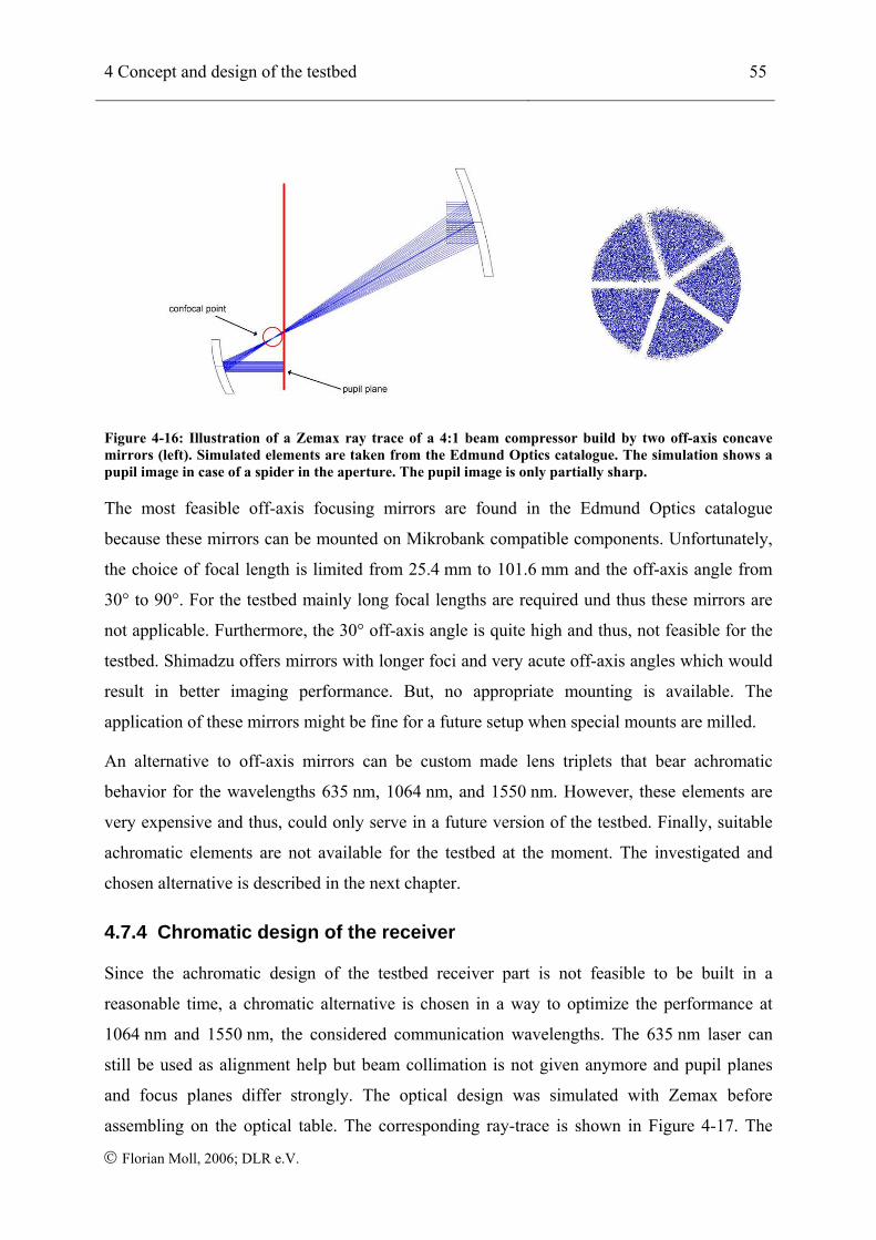
4 Concept and design of the testbed 55
© Florian Moll, 2006; DLR e.V.
Figure 4-16: Illustration of a Zemax ray trace of a 4:1 beam compressor build by two off-axis concave mirrors (left). Simulated elements are taken from the Edmund Optics catalogue. The simulation shows a pupil image in case of a spider in the aperture. The pupil image is only partially sharp.
The most feasible off-axis focusing mirrors are found in the Edmund Optics catalogue
because these mirrors can be mounted on Mikrobank compatible components. Unfortunately,
the choice of focal length is limited from 25.4 mm to 101.6 mm and the off-axis angle from
30° to 90°. For the testbed mainly long focal lengths are required und thus these mirrors are
not applicable. Furthermore, the 30° off-axis angle is quite high and thus, not feasible for the
testbed. Shimadzu offers mirrors with longer foci and very acute off-axis angles which would
result in better imaging performance. But, no appropriate mounting is available. The
application of these mirrors might be fine for a future setup when special mounts are milled.
An alternative to off-axis mirrors can be custom made lens triplets that bear achromatic
behavior for the wavelengths 635 nm, 1064 nm, and 1550 nm. However, these elements are
very expensive and thus, could only serve in a future version of the testbed. Finally, suitable
achromatic elements are not available for the testbed at the moment. The investigated and
chosen alternative is described in the next chapter.
4.7.4 Chromatic design of the receiver
Since the achromatic design of the testbed receiver part is not feasible to be built in a
reasonable time, a chromatic alternative is chosen in a way to optimize the performance at
1064 nm and 1550 nm, the considered communication wavelengths. The 635 nm laser can
still be used as alignment help but beam collimation is not given anymore and pupil planes
and focus planes differ strongly. The optical design was simulated with Zemax before
assembling on the optical table. The corresponding ray-trace is shown in Figure 4-17. The
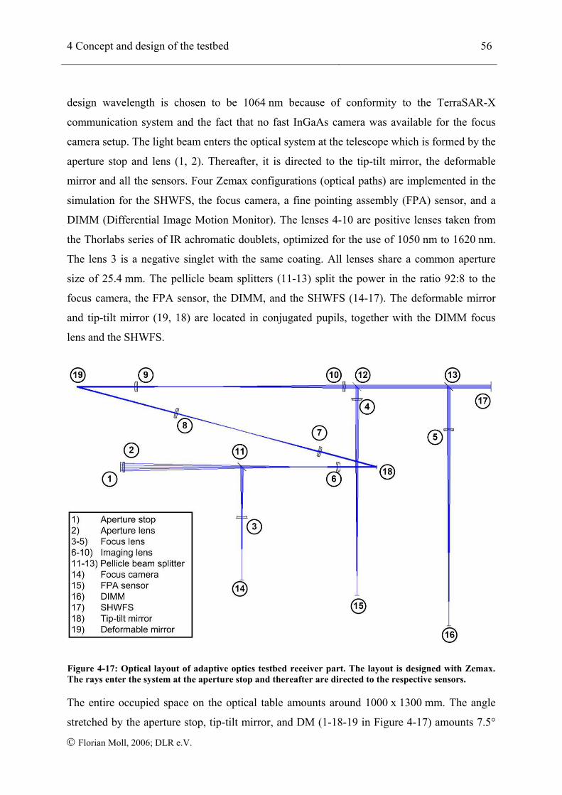
4 Concept and design of the testbed 56
© Florian Moll, 2006; DLR e.V.
design wavelength is chosen to be 1064 nm because of conformity to the TerraSAR-X
communication system and the fact that no fast InGaAs camera was available for the focus
camera setup. The light beam enters the optical system at the telescope which is formed by the
aperture stop and lens (1, 2). Thereafter, it is directed to the tip-tilt mirror, the deformable
mirror and all the sensors. Four Zemax configurations (optical paths) are implemented in the
simulation for the SHWFS, the focus camera, a fine pointing assembly (FPA) sensor, and a
DIMM (Differential Image Motion Monitor). The lenses 4-10 are positive lenses taken from
the Thorlabs series of IR achromatic doublets, optimized for the use of 1050 nm to 1620 nm.
The lens 3 is a negative singlet with the same coating. All lenses share a common aperture
size of 25.4 mm. The pellicle beam splitters (11-13) split the power in the ratio 92:8 to the
focus camera, the FPA sensor, the DIMM, and the SHWFS (14-17). The deformable mirror
and tip-tilt mirror (19, 18) are located in conjugated pupils, together with the DIMM focus
lens and the SHWFS.
Figure 4-17: Optical layout of adaptive optics testbed receiver part. The layout is designed with Zemax. The rays enter the system at the aperture stop and thereafter are directed to the respective sensors.
The entire occupied space on the optical table amounts around 1000 x 1300 mm. The angle
stretched by the aperture stop, tip-tilt mirror, and DM (1-18-19 in Figure 4-17) amounts 7.5°
4 Concept and design of the testbed 57
© Florian Moll, 2006; DLR e.V.
and thus, is in the range of the recommendation. The simulation misses the optical path of the
pupil camera, the fiber coupling and optical spare port as they are included in the testbed
concept described in chapter 4.2. But by adding additional beam splitters, the testbed design
as shown in Figure 4-17 may easily be extended.
Finally, this optical system is mounted on Linos Mikrobank parts and some custom made
mechanics whenever necessary. To identify correct positioning of the elements in the
conjugated pupils, a pupil camera is a good way to check. However, it is difficult to mark the
pupil position in a way that the respective element can be properly placed. Thus, this method
is very elaborate and not feasible for determining all pupil positions in the testbed. An easier
way is the placement of the elements just by distance measurements. This can be done if the
assembly strictly follows the Zemax simulation. Then, the distances of interest can be taken
from the Zemax layout. If all the lenses are mounted in their respective Mikrobank holders in
the same fashion, simple assembly rules can be derived. For that matter only the mounts have
to be placed correctly, however, with considering an offset between the lens vortex and the
mount edge. This offset can be calculated with knowledge of the dimensions of the lenses, the
Mikrobank holders, the lens rims and the lens rims rings.
The realization of the simulation in Figure 4-17 is shown in Figure 4-18. The beam enters the
system trough the aperture stop and lens (1). In general, the setup follows the system in the
simulation with the slight difference that the testbed on the optical table is assembled
horizontally symmetric to the simulation. Furthermore, the FPA sensor and the DIMM are not
mounted because no suitable devices were available. Due to image extent, the deformable
mirror is missing on the picture, but bears the mounting as depicted in Figure 4-12. The
utilized alignment helps can be seen on the bottom of the picture.
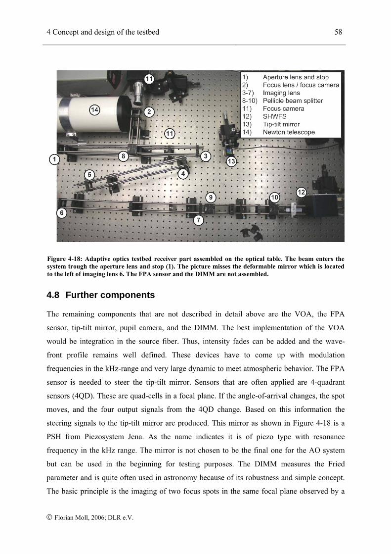
4 Concept and design of the testbed 58
© Florian Moll, 2006; DLR e.V.
Figure 4-18: Adaptive optics testbed receiver part assembled on the optical table. The beam enters the system trough the aperture lens and stop (1). The picture misses the deformable mirror which is located to the left of imaging lens 6. The FPA sensor and the DIMM are not assembled.
4.8 Further components
The remaining components that are not described in detail above are the VOA, the FPA
sensor, tip-tilt mirror, pupil camera, and the DIMM. The best implementation of the VOA
would be integration in the source fiber. Thus, intensity fades can be added and the wave-
front profile remains well defined. These devices have to come up with modulation
frequencies in the kHz-range and very large dynamic to meet atmospheric behavior. The FPA
sensor is needed to steer the tip-tilt mirror. Sensors that are often applied are 4-quadrant
sensors (4QD). These are quad-cells in a focal plane. If the angle-of-arrival changes, the spot
moves, and the four output signals from the 4QD change. Based on this information the
steering signals to the tip-tilt mirror are produced. This mirror as shown in Figure 4-18 is a
PSH from Piezosystem Jena. As the name indicates it is of piezo type with resonance
frequency in the kHz range. The mirror is not chosen to be the final one for the AO system
but can be used in the beginning for testing purposes. The DIMM measures the Fried
parameter and is quite often used in astronomy because of its robustness and simple concept.
The basic principle is the imaging of two focus spots in the same focal plane observed by a
4 Concept and design of the testbed 59
© Florian Moll, 2006; DLR e.V.
camera. The two spots are produced by placing a two-hole stop, where the whole diameter is
smaller than r0, in a pupil plane. A wedge behind this stop causes the two beams to differ in
angle and generates two spot images. The relative motion between these spots indicates the
strength of turbulence. Since the DIMM is considered to be located after the DM, the
remaining r0 can be measured. Finally, a pupil camera must be integrated in the testbed. Being
in synchronization with the focus camera, it should be possible to reconstruct the incident
wave. If in addition the SHWFS is in synchronization, the reconstructed wave can be
compared in different levels of resolution.
Finally, measurements of turbulence can be performed with the testbed setup described in the
preceding chapters.
5 Measurements and analysis 60
© Florian Moll, 2006; DLR e.V.
5 Measurements and analysis of the artificial turbulence
5.1 Measurement arrangement
The present chapter shows the results of the AoA measurements of the artificial turbulence,
how they are performed, and the analysis. The measurements are carried out with the testbed
setup described in Chapter 4. The 1064 nm diode laser served as input to the Newton
telescope. The collimated laser beam propagates through the hot-air OTG twice and the focus
images of the incident aberrated wave-front are captured by the focus camera. To reduce
possible disturbances, the laboratory lights have to be switched off, as well as the clean room
unit. Otherwise, their vibrations could influence the measurements. Furthermore, care must be
taken to prevent the images from being saturated. The distance between the OTG and the
receiver telescope amounts around 4.2 m. The aperture stop is formed by an iris diaphragm
and is set to 15 mm diameter. By tuning the power dimmer, the temperature of the hot-air
intake is adjusted. The measurements are performed with a frame rate of 720 Hz and exposure
time of around 1.39 ms (the inverse of the frame rate). All measurements are running for 20
seconds are performed five times for a given OTG parameterization. Eventually, the particular
measurements consist of 14 400 images each. From these images, two different metrics are
derived. The first is the long-time exposure image, which is generated by calculating the mean
of all images. The second one is the angle-of-arrival of the incident wave-front in x- and y-
direction for each short-term exposure image.
All the measurements, the single images, are stored in a folder structure with the respective
measurement protocol and descriptive file and folder names.
A calibration of the OTG is important to use it for communication and adaptive optics
systems tests without having to do turbulence measurements each time. Since the temperature
difference Tdiff determines the strength of turbulence, a calibration curve of temperature
difference over dimmer scale of the power dimmer scale (DS) is recorded and illustrated in
Figure 5-1. The dependency of Tdiff from DS is quite linear. Unfortunately, with the applied
Voltcraft T-300 thermometers on top of the OTG, as illustrated in Figure 4-4, temperature
measurements can only be performed at a single point of the particular air flows. The test
prods of the thermometers are approximately located in the center of the flows. The problem
here is that the values of the two-dimensional temperature field of the particular flow may
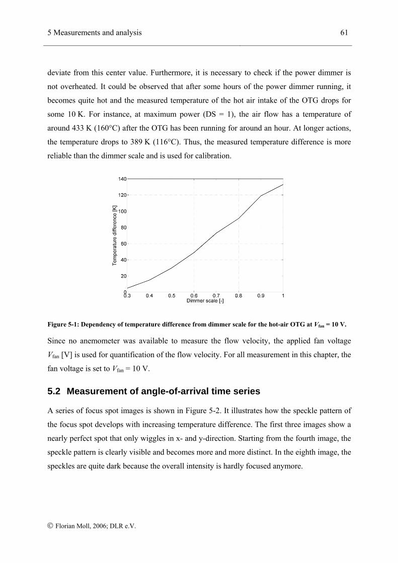
5 Measurements and analysis 61
© Florian Moll, 2006; DLR e.V.
deviate from this center value. Furthermore, it is necessary to check if the power dimmer is
not overheated. It could be observed that after some hours of the power dimmer running, it
becomes quite hot and the measured temperature of the hot air intake of the OTG drops for
some 10 K. For instance, at maximum power (DS = 1), the air flow has a temperature of
around 433 K (160°C) after the OTG has been running for around an hour. At longer actions,
the temperature drops to 389 K (116°C). Thus, the measured temperature difference is more
reliable than the dimmer scale and is used for calibration.
Figure 5-1: Dependency of temperature difference from dimmer scale for the hot-air OTG at Vfan = 10 V.
Since no anemometer was available to measure the flow velocity, the applied fan voltage
Vfan [V] is used for quantification of the flow velocity. For all measurement in this chapter, the
fan voltage is set to Vfan = 10 V.
5.2 Measurement of angle-of-arrival time series
A series of focus spot images is shown in Figure 5-2. It illustrates how the speckle pattern of
the focus spot develops with increasing temperature difference. The first three images show a
nearly perfect spot that only wiggles in x- and y-direction. Starting from the fourth image, the
speckle pattern is clearly visible and becomes more and more distinct. In the eighth image, the
speckles are quite dark because the overall intensity is hardly focused anymore.

5 Measurements and analysis 62
© Florian Moll, 2006; DLR e.V.
1) Tdiff = 5°C 2) Tdiff = 15°C 3) Tdiff = 30°C 4) Tdiff = 49°C
5) Tdiff = 73°C 6) Tdiff = 91°C 7) Tdiff = 119°C 8) Tdiff = 133 K
Figure 5-2: Image series for increasing temperature difference and Vfan = 10 V as captured by the focus camera. With increasing Tdiff, the speckle pattern of the spot becomes more distinct.
The corresponding time series of the eight angle-of-arrival measurements with increasing Tdiff
is plotted in Figure 5-3. The AoA stroke increases with Tdiff which indicates higher
turbulence. Since the AoA shows high peak events, extreme situations can be tested well.
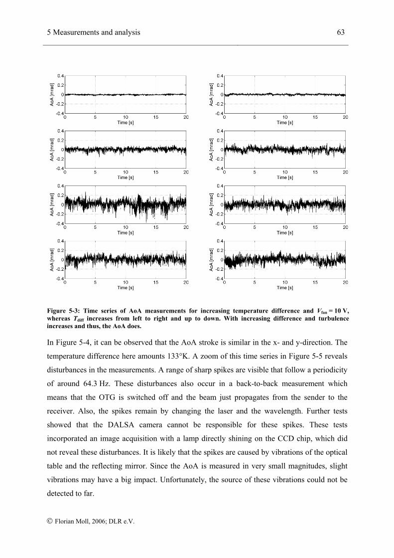
5 Measurements and analysis 63
© Florian Moll, 2006; DLR e.V.
Figure 5-3: Time series of AoA measurements for increasing temperature difference and Vfan = 10 V, whereas Tdiff increases from left to right and up to down. With increasing difference and turbulence increases and thus, the AoA does.
In Figure 5-4, it can be observed that the AoA stroke is similar in the x- and y-direction. The
temperature difference here amounts 133°K. A zoom of this time series in Figure 5-5 reveals
disturbances in the measurements. A range of sharp spikes are visible that follow a periodicity
of around 64.3 Hz. These disturbances also occur in a back-to-back measurement which
means that the OTG is switched off and the beam just propagates from the sender to the
receiver. Also, the spikes remain by changing the laser and the wavelength. Further tests
showed that the DALSA camera cannot be responsible for these spikes. These tests
incorporated an image acquisition with a lamp directly shining on the CCD chip, which did
not reveal these disturbances. It is likely that the spikes are caused by vibrations of the optical
table and the reflecting mirror. Since the AoA is measured in very small magnitudes, slight
vibrations may have a big impact. Unfortunately, the source of these vibrations could not be
detected to far.
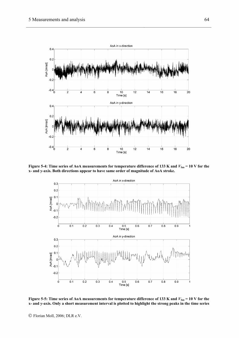
5 Measurements and analysis 64
© Florian Moll, 2006; DLR e.V.
Figure 5-4: Time series of AoA measurements for temperature difference of 133 K and Vfan = 10 V for the x- and y-axis. Both directions appear to have same order of magnitude of AoA stroke.
Figure 5-5: Time series of AoA measurements for temperature difference of 133 K and Vfan = 10 V for the x- and y-axis. Only a short measurement interval is plotted to highlight the strong peaks in the time series
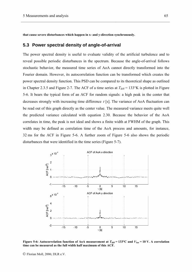
5 Measurements and analysis 65
© Florian Moll, 2006; DLR e.V.
that cause severe disturbances which happen in x- and y-direction synchronously.
5.3 Power spectral density of angle-of-arrival
The power spectral density is useful to evaluate validity of the artificial turbulence and to
reveal possible periodic disturbances in the spectrum. Because the angle-of-arrival follows
stochastic behavior, the measured time series of AoA cannot directly transformed into the
Fourier domain. However, its autocorrelation function can be transformed which creates the
power spectral density function. This PSD can be compared to its theoretical shape as outlined
in Chapter 2.3.5 and Figure 2-7. The ACF of a time series at Tdiff = 133°K is plotted in Figure
5-6. It bears the typical form of an ACF for random signals: a high peak in the center that
decreases strongly with increasing time difference τ [s]. The variance of AoA fluctuation can
be read out of this graph directly as the center value. The measured variance meets quite well
the predicted variance calculated with equation 2.30. Because the behavior of the AoA
correlates in time, the peak is not ideal and shows a finite width at FWHM of the graph. This
width may be defined as correlation time of the AoA process and amounts, for instance,
32 ms for the ACF in Figure 5-6. A further zoom of Figure 5-6 also shows the periodic
disturbances that were identified in the time series (Figure 5-7).
Figure 5-6: Autocorrelation function of AoA measurement at Tdiff = 133°C and Vfan = 10 V. A correlation time can be measured as the full width half maximum of this ACF.
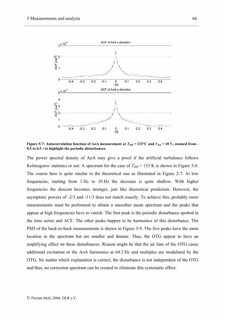
5 Measurements and analysis 66
© Florian Moll, 2006; DLR e.V.
Figure 5-7: Autocorrelation function of AoA measurement at Tdiff = 133°C and Vfan = 10 V, zoomed from -0.5 to 0.5 τ to highlight the periodic disturbances.
The power spectral density of AoA may give a proof if the artificial turbulence follows
Kolmogorov statistics or not. A spectrum for the case of Tdiff = 133 K is shown in Figure 5-8.
The course here is quite similar to the theoretical one as illustrated in Figure 2-7. At low
frequencies, starting from 1 Hz to 10 Hz the decrease is quite shallow. With higher
frequencies the descent becomes stronger, just like theoretical prediction. However, the
asymptotic powers of -2/3 and -11/3 does not match exactly. To achieve this, probably more
measurements must be performed to obtain a smoother mean spectrum and the peaks that
appear at high frequencies have to vanish. The first peak is the periodic disturbance spotted in
the time series and ACF. The other peaks happen to be harmonics of this disturbance. The
PSD of the back-to-back measurements is shown in Figure 5-9. The five peaks have the same
location in the spectrum but are smaller and thinner. Thus, the OTG appear to have an
amplifying effect on these disturbances. Reason might be that the air fans of the OTG cause
additional excitation or the AoA harmonics at 64.3 Hz and multiples are modulated by the
OTG. No matter which explanation is correct, the disturbance is not independent of the OTG
and thus, no correction spectrum can be created to eliminate this systematic effect.
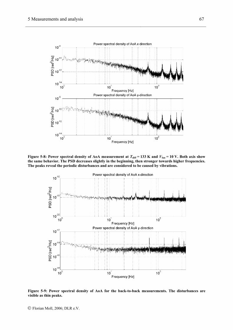
5 Measurements and analysis 67
© Florian Moll, 2006; DLR e.V.
Figure 5-8: Power spectral density of AoA measurement at Tdiff = 133 K and Vfan = 10 V. Both axis show the same behavior. The PSD decreases slightly in the beginning, then stronger towards higher frequencies. The peaks reveal the periodic disturbances and are considered to be caused by vibrations.
Figure 5-9: Power spectral density of AoA for the back-to-back measurements. The disturbances are visible as thin peaks.
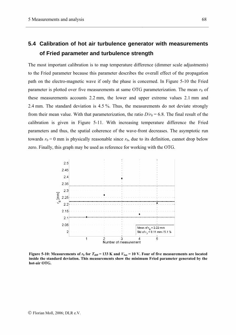
5 Measurements and analysis 68
© Florian Moll, 2006; DLR e.V.
5.4 Calibration of hot air turbulence generator with measurements of Fried parameter and turbulence strength
The most important calibration is to map temperature difference (dimmer scale adjustments)
to the Fried parameter because this parameter describes the overall effect of the propagation
path on the electro-magnetic wave if only the phase is concerned. In Figure 5-10 the Fried
parameter is plotted over five measurements at same OTG parameterization. The mean r0 of
these measurements accounts 2.2 mm, the lower and upper extreme values 2.1 mm and
2.4 mm. The standard deviation is 4.5 %. Thus, the measurements do not deviate strongly
from their mean value. With that parameterization, the ratio D/r0 = 6.8. The final result of the
calibration is given in Figure 5-11. With increasing temperature difference the Fried
parameters and thus, the spatial coherence of the wave-front decreases. The asymptotic run
towards r0 = 0 mm is physically reasonable since r0, due to its definition, cannot drop below
zero. Finally, this graph may be used as reference for working with the OTG.
Figure 5-10: Measurements of r0 for Tdiff = 133 K and Vfan = 10 V. Four of five measurements are located inside the standard deviation. This measurements show the minimum Fried parameter generated by the hot-air OTG.
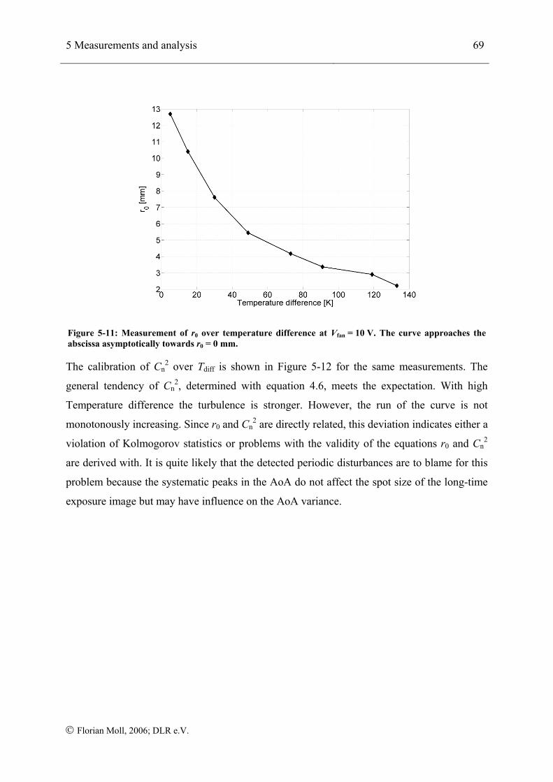
5 Measurements and analysis 69
© Florian Moll, 2006; DLR e.V.
Figure 5-11: Measurement of r0 over temperature difference at Vfan = 10 V. The curve approaches the abscissa asymptotically towards r0 = 0 mm.
The calibration of Cn2 over Tdiff is shown in Figure 5-12 for the same measurements. The
general tendency of Cn2, determined with equation 4.6, meets the expectation. With high
Temperature difference the turbulence is stronger. However, the run of the curve is not
monotonously increasing. Since r0 and Cn2 are directly related, this deviation indicates either a
violation of Kolmogorov statistics or problems with the validity of the equations r0 and Cn2
are derived with. It is quite likely that the detected periodic disturbances are to blame for this
problem because the systematic peaks in the AoA do not affect the spot size of the long-time
exposure image but may have influence on the AoA variance.
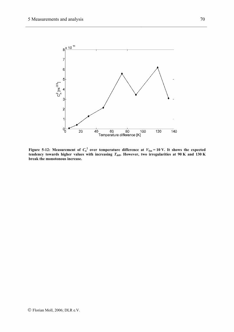
5 Measurements and analysis 70
© Florian Moll, 2006; DLR e.V.
Figure 5-12: Measurement of Cn2 over temperature difference at Vfan = 10 V. It shows the expected
tendency towards higher values with increasing Tdiff. However, two irregularities at 90 K and 130 K break the monotonous increase.
6 Conclusion 71
© Florian Moll, 2006; DLR e.V.
6 Conclusion
The development of the adaptive optics testbed incorporated many different issues. These
include the theory of atmospheric turbulence and its measurement, the principle of wave-front
sensors, deformable mirrors, tip-tilt mirrors, optical imaging, and generation of artificial
turbulence. All issues were embedded successfully in the design of the AO testbed. For that
matter, an overall concept of an AO testbed was developed. The most important parts of this
concept were set up and implemented. Eventually, it is ready for use and may give support in
investigating adaptive optics systems, wave-front sensing techniques, tracking techniques, and
communication schemes.
As basis for the work the relevant turbulence theory and its effects on FSO systems was
investigated. Afterwards, the requirements on the testbed concept, the optical turbulence
generator, the deformable mirror, and the overall optical design could be set.
A most suitable deformable mirror was identified, that is expected to fulfill the needs, and
implemented in the testbed.
An optical setup was developed that allows an AO system to be driven and furthermore offers
the possibility to test new ideas in the lab before going to the field for experiments. Although,
the optical design was planned to be achromatic for 635 nm, 1064 nm, and 1550 nm, this
requirement had to be skipped due to higher expense and lack of time and instead, a chromatic
version was built. However, ideas are presented to gain achromatic performance if needed.
Especially the OTG and its characterization were of major concern. A first version was
developed, built, and tested. A calibration of Fried parameter dependent on temperature
difference in the OTG is achieved. With a wavelength of 1064 nm measurements of the long-
term focus spot and the angle-of-arrival of the incoming wave were performed. The size of r0
could be reduced to 2.2 mm and thus, a realistic ratio D/r0 can be created. However, an
unexpected periodic behavior could be detected in the measurements of angle-of-arrival that
cause peaks in the angle-of-arrival spectrum at around 65 Hz and harmonics. This is quite
likely the reason why the measured Fried parameter and turbulence strength are not perfectly
correlated.
For the further development of the testbed some more suggestions may be given here. These
are the application of a faster focus camera to measure a broader power spectral density of the
6 Conclusion 72
© Florian Moll, 2006; DLR e.V.
angle-of-arrival. The detected periodic disturbances have to be eliminated to get rid of the
peaks at the high frequencies. If vibrations are the reason, it is feasible to eliminate their
origin by mounting the optical table and reflecting mirror on air bases to absorb those.
Furthermore, it is valuable to use a synchronized pupil camera together with the focus camera
to test further phase retrieval methods besides classical wave-front sensors. A future
improvement of the optics may be the implementation of a larger aperture lens which
increases the important ratio D/r0. Regarding the OTG, a version with a bigger mixing
chamber and higher temperature difference can be built to achieve stronger turbulence. It also
makes sense to set up a cascade of OTGs simulating several atmospheric layers.
References 73
© Florian Moll, 2006; DLR e.V.
References
[Abt06] M. Abtahi, P. Lemieux, W. Mathlouthi, and L. A. Rusch, “Suppression of turbulence-induced scintillation in free-space optical communication systems using saturated optical amplifiers,” Journal of Lightwave Technology, vol. 24, no. 12, pp. 4966-4973, December 2006.
[And05] L. C. Andrews and R. L. Philips, Laser beam propagation through random media. Bellingham: SPIE Press, 2005.
[Bur08] L. Burger, I. Litvin, and A. Forbes, "Simulating atmospheric turbulence using a phase-only spatial light modulator," in South African Journal of Science, vol. 104, 2008, pp. 129-134.
[Con95] J. M. Conan, G. Rousset, P.Y. Madec, "Wave-front temporal spectra in high-resolution imaging through turbulence," in Journal of the Optical Society of America A: Optics, Image Science, and Vision, Volume 12, Issue 7, 1995, pp. 1559-1570.
[Dev08] N. Devaney, D. Coburn, C. Coleman, C. Dainty, E. Dalimier, T. Farrell, D.
Lara, D. Mackey, and R. Mackey, “Characterization of MEMs for use in
atmospheric and ocular wave-front correction,“ in Proceedings of SPIE,
vol. 6888, 2008, pp. 68882-1 - 68882-10.
[Dik05] Y. Dikmelik and F. M. Davidson, “Fiber-coupling efficiency for free space optical communication through atmospheric turbulence,“ Applied Optics, vol. 44, no. 23, pp. 4946-4952, August 2005.
[Far07] T. Farell, E. Daly, E. Dalimier, and Chris Dainty, “Task-based assessment of deformable mirrors,” in Proceedings of SPIE, vol. 6467, 2007, pp. 64670F.1-64670F.7.
[Fri67] D. L. Fried, “Optical heterodyne detection of an atmospherically distorted signal Wave-front,” in Proceedings of the IEEE, vol. 55, 1967, pp. 57-67.
[Fuc96] A. Fuchs, J. Vernin, and M. Tallon, “Laboratory simulation of a turbulent layer: Optical and in situ characterization,“ Applied Optics, vol. 35, no. 10, pp. 1751-1755, Aptil 1996.
[Gam78] H. Gamo and A. K. Majumdar, “Atmospheric turbulence chamber for optical transmission experiment: Characterization by thermal method, “Applied Optics, vol. 17, no. 23, pp. 3755-3762, December 1978.
[Gea95] J. M. Geary: Introduction to Wave-front Sensors. Bellingham: SPIE Optical Engineering Press, 1995.
References 74
© Florian Moll, 2006; DLR e.V.
[Gig04] D. Giggenbach, “Optimierung der optischen Freiraumkommunikation durch die Atmosphäre - Focal array receiver,“ Ph.D. dissertation, Universität der Bundeswehr München, Munic, Germany, 2004.
[Gli97] A. Glindemann, "Relevant parameters for the tip-tilt systems on large telescopes," in Publications of the Astronomical Society of the Pacific, Volume 109, 1997, pp. 682-687.
[Gli97a] A. Glindemann, “Beating the seeing limit – Adaptive optics on large telescopes,“ habilitation treatise, Ruprecht-Karls-Universität, Heidelberg, Germany, 1997.
[Gm09] GM GmbH, “Technisches Know-How Kunststoffe & Datenblätter,” May 2009, http://www.gm-gmbh.de/index.php?p=6&s=7.
[Gre77] D. P. Greenwood, “Bandwidth specification for adaptive optics systems,” in Journal of the Optical Society of America A: Optics, Image Science, and Vision, Volume 67, Issue 3, 1977, pp. 390-393.
[Hec05] E. Hecht, Optik. Munic: Oldenburg Wissenschaftsverlag GmbH, 2005.
[Hor07] J. Horwath, N. Perlot; M. Knapek and F. Moll, “Experimental verification of optical backhaul links for high-altitude platform networks: Atmospheric turbulence and downlink availability,” International Journal of Satellite Communications and Networking, vol. 25, pp. 501-528, 2007.
[Jol06] L. Jolissaint, “Optical turbulence generators for testing astronomical adaptive optics systems: a review and designer guide,” The Publications of the Astronomical Society of the Pacific, vol. 118, pp. 1205-1224, 2006.
[Jol08] L. Jolissaint (private communication), 2008.
[Kes06] O. Keskin, L. Laurent, and C. Bradley, “Hot-air optical turbulence generator for the testing of adaptive optics systems: principles and characterization,“ Applied Optics, vol. 45, no. 20, pp. 4888-4897, July 2006.
[Kna09] M. Knapek, J. Horwath, and N. Perlot, Manhart, “Atmospheric measurements in downlink experiments from TerraSAR-X – Final report,“ ESTEC Contr. No.: 18252/04/NL/PM, 2009.
[Kol91] A. N. Kolmogorov, “The local structure of turbulence in incompressible fluids for very large Reynolds numbers,” Proceedings of the Royal Society of London A, vol. 434, pp. 9-13, July 1991.
[Kol04] J. Kolb, “MAPS, a turbulence simulator for MCAO,“ in Proceedings of SPIE, vol. 5490, 2004, pp. 794-804.
[Lic08] University of California Observatories, Lick Observatory, “User’s guide to the adaptive optics system,” January 2008,
References 75
© Florian Moll, 2006; DLR e.V.
http://mthamilton.ucolick.org/techdocs/instruments/AO/ao_optics.html.
[Mah83] V. N. Mahajan, "Strehl ratio for primary aberrations in terms of their aberration variance," in Journal of the Optical Society of America A: Optics, Image Science, and Vision, Volume 73, Issue 6, 1983, pp. 860-861.
[Maj82] A. K. Majumdar and H. Gamo, “Statistical measurements of irradiance fluctuations of a multipass laser beam propagated through laboratory-simulated atmospheric turbulence, “Applied Optics, vol. 21, no. 12, pp. 2229-2235, June 1978.
[Maj98] A. K. Majumdar, “Laboratory simulation of atmospheric turbulence for laser propagation: Design and characterization,“ in Proceedings of SPIE, vol. 3432, 1998, pp. 50-56.
[Nol76] R. Noll, "Zernike polynomials and atmospheric turbulence," in Journal of the Optical Society of America A: Optics, Image Science, and Vision, Volume 66, Issue 6, 1976, pp. 207-211.
[Per05] N. Perlot, “Characterization of Signal Fluctuations in Optical Communications with Intensity Modulation and Direct Detection through the Turbulent Atmospheric Channel,” Ph.D. dissertation, University of Valenciennes and Hainaut-Cambrésis, Valenciennes, France, 2005.
[Per07] N. Perlot, “The Kirari optical downlink to Oberpfaffenhofen (KIODO),” German Aerospace Center (DLR), Weßling, Germany, Report on DLR-JAXA Joint Experiment, 2007.
[Mac08] R. Mackey (private communication), December, 2008.
[Smi96] F. G. Smith, Atmospheric propagation of radiation - the infrared and electro-optical systems handbook. Bellingham: SPIE Press, 1996.
[Sod07] Z. Sodnik, “Status of laser communication in Europe,” presented at 13th Ka and Broadband Communications Conference, Torino, Italy, 2007.
[Tyl94] G. A. Tyler, “Bandwidth considerations for tracking through strong turbulence,” in Journal of the Optical Society of America A: Optics, Image Science, and Vision, Volume 11, Issue 1, 1992, pp. 358-367.
[Tys00] R. K. Tyson, Introduction to Adaptive Optics. Bellingham: SPIE Press, 2000.
[Wag82] R. E. Wagner and W. J. Tomlinson: Coupling efficiency of optics in single-mode fiber components. Applied Optics, Vol. 21, No. 15, 1982.
[Wei74] G. P. Weigelt: “Large field speckle interferometry,” Optik, vol. 43, pp. 111-128, 1974.
[Wiz06] P. L. Wizinowich et al.: “The W. M. Keck observatory laser guide star
References 76
© Florian Moll, 2006; DLR e.V.
adaptive optics system: Overview,” Publications of the Astronomical Society of the Pacific, vol. 118, pp. 297-309, 2006.
Appendix 77
© Florian Moll, 2006; DLR e.V.
Appendix
A Wind speed
The rms wind speed in equation 2.5 is determined from
3
3
1 220 10 2
rms 3 5 10
1 ( )15 10
v v h dh⋅
⋅
⎡ ⎤= ⎢ ⎥⋅⎣ ⎦∫ , A.1
where v(h) is often described by the Bufton wind model, which is expressed with
2
s g9400( ) 30 exp
4800hv h h vω
⎡ ⎤−⎛ ⎞= + + ⋅ −⎢ ⎥⎜ ⎟⎝ ⎠⎢ ⎥⎣ ⎦
. A.2
The quantity vg [m/s] is the ground wind speed and ωs [rad/s] is the slew rate associated with a
satellite moving with respect to an observer on the ground. The slew rate becomes important
in making temporal calculations [And05]. Figure A.1 contains an example of wind profile and
illustrates the additional pseudo wind component due to satellite motion for a zenith viewing
angle. The sum of both results in the effective transversal wind speed. In height of the jet
streams the real wind has its highest contribution. Over 20 km, the transversal wind speed is
almost completely determined by the satellite motion. This effect increases for lower viewing
angles. With a ground station at 600 m and a vg of 5 m/s the resulting vrms amounts 23 m/s
which can be used in equation 2.5 to create the Cn2 profile.
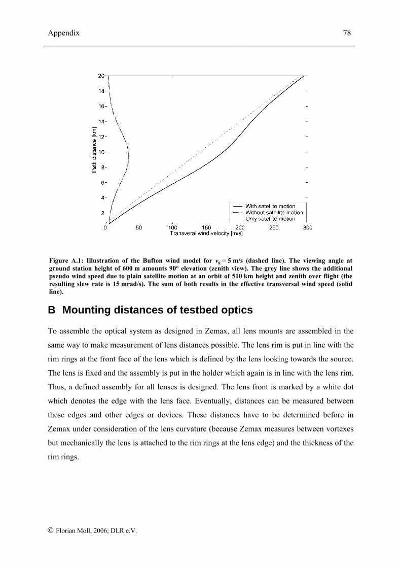
Appendix 78
© Florian Moll, 2006; DLR e.V.
Figure A.1: Illustration of the Bufton wind model for vg = 5 m/s (dashed line). The viewing angle at ground station height of 600 m amounts 90° elevation (zenith view). The grey line shows the additional pseudo wind speed due to plain satellite motion at an orbit of 510 km height and zenith over flight (the resulting slew rate is 15 mrad/s). The sum of both results in the effective transversal wind speed (solid line).
B Mounting distances of testbed optics
To assemble the optical system as designed in Zemax, all lens mounts are assembled in the
same way to make measurement of lens distances possible. The lens rim is put in line with the
rim rings at the front face of the lens which is defined by the lens looking towards the source.
The lens is fixed and the assembly is put in the holder which again is in line with the lens rim.
Thus, a defined assembly for all lenses is designed. The lens front is marked by a white dot
which denotes the edge with the lens face. Eventually, distances can be measured between
these edges and other edges or devices. These distances have to be determined before in
Zemax under consideration of the lens curvature (because Zemax measures between vortexes
but mechanically the lens is attached to the rim rings at the lens edge) and the thickness of the
rim rings.
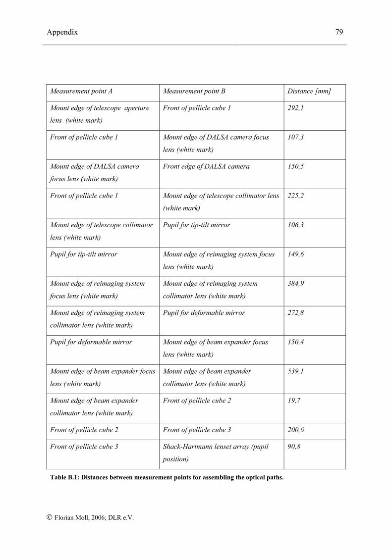
Appendix 79
© Florian Moll, 2006; DLR e.V.
Measurement point A Measurement point B Distance [mm]
Mount edge of telescope aperture
lens (white mark)
Front of pellicle cube 1 292,1
Front of pellicle cube 1 Mount edge of DALSA camera focus
lens (white mark)
107,3
Mount edge of DALSA camera
focus lens (white mark)
Front edge of DALSA camera 150,5
Front of pellicle cube 1 Mount edge of telescope collimator lens
(white mark)
225,2
Mount edge of telescope collimator
lens (white mark)
Pupil for tip-tilt mirror 106,3
Pupil for tip-tilt mirror Mount edge of reimaging system focus
lens (white mark)
149,6
Mount edge of reimaging system
focus lens (white mark)
Mount edge of reimaging system
collimator lens (white mark)
384,9
Mount edge of reimaging system
collimator lens (white mark)
Pupil for deformable mirror 272,8
Pupil for deformable mirror Mount edge of beam expander focus
lens (white mark)
150,4
Mount edge of beam expander focus
lens (white mark)
Mount edge of beam expander
collimator lens (white mark)
539,1
Mount edge of beam expander
collimator lens (white mark)
Front of pellicle cube 2 19,7
Front of pellicle cube 2 Front of pellicle cube 3 200,6
Front of pellicle cube 3 Shack-Hartmann lenset array (pupil
position)
90,8
Table B.1: Distances between measurement points for assembling the optical paths.
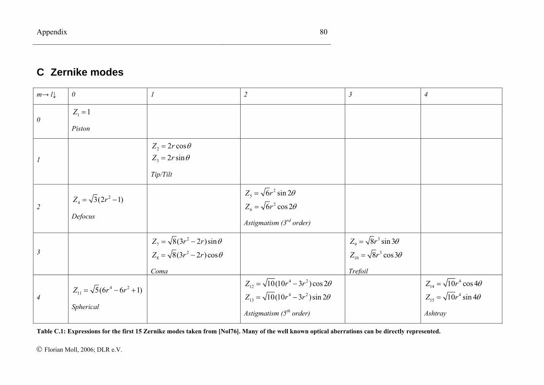
Appendix 80
© Florian Moll, 2006; DLR e.V.
C Zernike modes
m→ l↓ 0 1 2 3 4
0 1 1Z =
Piston
1 2
3
2 cos2 sin
Z rZ r
θθ
==
Tip/Tilt
2 2
4 3(2 1)Z r= −
Defocus
25
26
6 sin 2
6 cos 2
Z r
Z r
θ
θ
=
=
Astigmatism (3rd order)
3
27
28
8(3 2 )sin
8(3 2 )cos
Z r r
Z r r
θ
θ
= −
= −
Coma
39
310
8 sin 3
8 cos3
Z r
Z r
θ
θ
=
=
Trefoil
4 4 2
11 5(6 6 1)Z r r= − +
Spherical
4 212
4 213
10(10 3 )cos 2
10(10 3 )sin 2
Z r r
Z r r
θ
θ
= −
= −
Astigmatism (5th order)
414
415
10 cos 4
10 sin 4
Z r
Z r
θ
θ
=
=
Ashtray
Table C.1: Expressions for the first 15 Zernike modes taken from [Nol76]. Many of the well known optical aberrations can be directly represented.

© Florian Moll, 2006; DLR e.V.