MASTER THESISluismatias.addvolt.com/lib/exe/fetch.php?media=... · ratories Europe collaborates with NEC’s global research organizations in Japan, China, Singapore and The United

Department of Computer Science (Intelligent Systems)

MASTER THESIS

Ranking Feature Importance ThroughRepresentation Hierarchies

Sourabh Sarvotham Parkala (399431)

April 16, 2018

MASTER THESIS

Ranking Feature Importance ThroughRepresentation Hierarchies

Personal Details:

Author : Sourabh Sarvotham ParkalaStudent Number : 399431Email Id : [email protected] : Masters in Computer ScienceSpecialization : Intelligent Systems

Supervising Professor: apl. Prof. Dr. habil. Marcus Liwicki(Technische Universitat Kaiserslautern)

Supervisor: Dr. Luis Moreira-Matias(NEC Laboratories Europe GmbH, Heidelberg)

Acknowledgement

This thesis is submitted in partial fulfillment of the requirements for the degree of Master of Sciencein Computer Science at Technische Universitat Kaiserslautern. It has been carried out at NECLaboratories Europe Gmbh, Heidelberg.

I am extremely grateful to Prof. Dr. habil. Marcus Liwicki for guiding and providing mewith all the valuable inputs to help me excel in my Master Thesis. He has always motivated metowards more intensive research work which helped me immensely in exploring the bigger picture ofthings.

I would also like to express my sincere gratitude to Dr. Luis Moreira-Matias for his excel-lent guidance and patience. I feel really privileged to have him as my supervisor. He has alwaysencouraged me to try and explore new ideas for the betterment of things. I would like to thankall my colleagues, especially Jihed Khiari and Xiao He at NEC Laboratories Europe GmbH, forrendering me their immense support and valuable suggestions.

Last but not the least, I would like to thank my family and all my friends for their constantsupport and encouragement, throughout my studies, without which this work would not have beenpossible.

i

Declaration

I hereby declare that this thesis is a report of my research and has been written by me. The col-laborative contributions have been indicated clearly and acknowledged. Due references have beenprovided on all supporting literature and resources. Where I have consulted the published work ofothers, it is clearly stated and cited. I have acknowledged all main source of help.

Kaiserslautern, 16th April 2018

...............................................................................................................................................................................................................................................................................................................................Parkala, Sourabh Sarvotham

ii

Preface

NEC Laboratories Europe (NLE) GmbH located in Heidelberg, Germany was established in 1994with special emphasis on solutions meeting the needs of NEC’s European customers. NEC Labo-ratories Europe collaborates with NEC’s global research organizations in Japan, China, Singaporeand The United States, as well as with NEC’s business units.

NEC Laboratories Europe Gmbh focuses on software-oriented research and development of tech-nologies to enable advanced Information and Communications Technology (ICT)-based solutions forsociety. Solution areas include smart cities, public transport and safety, digital health using theInternet of Things (IoT). It is achieved by intensive research on technologies for machine learning,automated reasoning, blockchain technology, IoT security, edge computing, network virtualizationand automation [1].

iii

Abstract

Nowadays, the production-grade software contains one or more Predictive Analytics components.Predictive Analytics is a branch of analytics which is used to make predictions about the unknownfuture events. The predictive analytics components rely on complex stepwise Machine Learningpipelines, particularly designed and tuned for an application of interest. Such tasks are heavilydependent on the human expertise, narrowing the pool of possible users to those who master thisart.

This thesis work provides an overview of techniques typically used to address three steps of thispipeline: Feature Engineering, Feature Selection and Hyperparameter Tuning. We introduce Auto-Tune: a framework to address these steps, all at once for supervised learning problems conductedover structured data.

Our main contribution is on providing local interpretability to the models tuned by AutoTune.We do it so by extending recent work on Local Interpretable Model-Agnostic Explanations (LIME)to provide explanations over the raw features (which is easily interpretable by application domainexperts) instead of the abstract representations of features (hierarchical features obtained from theraw features) used by the final Machine Learning models to output the predictions.

An exhaustive test bed was conducted over a regression problem from the transportation domainrelying on the real-world dataset. The obtained results illustrate the contributions of the proposedframework.

Keywords— Automated Machine Learning, Feature Selection, Bayesian Alternated Model Se-lection, Ensemble Model Selection, Travel Time Prediction, Random Forest, Support Vector Ma-chine, Project Pursuit Regression, Neural Network, Gradient Boost Machine, Feature Hierarchies,Local interpretable model-agnostic explanations, LIME

iv

Contents

Acknowledgement i

Declaration ii

Preface iii

Abstract iv

List of Figures vii

List of Tables viii

Acronyms ix

1 Introduction 11.1 Problem Statement . . . . . . . . . . . . . . . . . . . . . . . . . . . . . . . . . . . . . 21.2 Motivation . . . . . . . . . . . . . . . . . . . . . . . . . . . . . . . . . . . . . . . . . 21.3 Aim . . . . . . . . . . . . . . . . . . . . . . . . . . . . . . . . . . . . . . . . . . . . . 31.4 Structure of Thesis . . . . . . . . . . . . . . . . . . . . . . . . . . . . . . . . . . . . . 3

2 Literature Review 42.1 Selection of Adequate Features . . . . . . . . . . . . . . . . . . . . . . . . . . . . . . 42.2 Representation Learning of Features . . . . . . . . . . . . . . . . . . . . . . . . . . . 42.3 Hyperparameter Tuning . . . . . . . . . . . . . . . . . . . . . . . . . . . . . . . . . . 52.4 Explain Model Interpretations . . . . . . . . . . . . . . . . . . . . . . . . . . . . . . . 6

3 Prerequisite Knowledge 73.1 Random Forests (RF) . . . . . . . . . . . . . . . . . . . . . . . . . . . . . . . . . . . 73.2 Support Vector Machines (SVM) . . . . . . . . . . . . . . . . . . . . . . . . . . . . . 83.3 Projection Pursuit Regression (PPR) . . . . . . . . . . . . . . . . . . . . . . . . . . . 103.4 Gradient Boost Machine (GBM) . . . . . . . . . . . . . . . . . . . . . . . . . . . . . 103.5 Neural Network (NN) . . . . . . . . . . . . . . . . . . . . . . . . . . . . . . . . . . . 113.6 Local Interpretable Model-Agnostic Explanations (LIME) . . . . . . . . . . . . . . . 13

4 Domain Application 154.1 Transit Management Systems (TMS) . . . . . . . . . . . . . . . . . . . . . . . . . . . 154.2 Travel Time Prediction (TTP) . . . . . . . . . . . . . . . . . . . . . . . . . . . . . . 154.3 Case Study and Preprocessing . . . . . . . . . . . . . . . . . . . . . . . . . . . . . . . 17

4.3.1 Case Study . . . . . . . . . . . . . . . . . . . . . . . . . . . . . . . . . . . . . 174.3.2 Feature Preprocessing . . . . . . . . . . . . . . . . . . . . . . . . . . . . . . . 19

5 Methodology 205.1 AutoTune . . . . . . . . . . . . . . . . . . . . . . . . . . . . . . . . . . . . . . . . . . 20

5.1.1 Feature Generation . . . . . . . . . . . . . . . . . . . . . . . . . . . . . . . . . 225.1.2 Feature Explosion . . . . . . . . . . . . . . . . . . . . . . . . . . . . . . . . . 235.1.3 Feature Selection . . . . . . . . . . . . . . . . . . . . . . . . . . . . . . . . . . 245.1.4 Model Selection . . . . . . . . . . . . . . . . . . . . . . . . . . . . . . . . . . . 24

v

5.1.5 Postprocessing . . . . . . . . . . . . . . . . . . . . . . . . . . . . . . . . . . . 245.2 Feature Selection Techniques . . . . . . . . . . . . . . . . . . . . . . . . . . . . . . . 25

5.2.1 LASSO - baseline for Feature Selection . . . . . . . . . . . . . . . . . . . . . . 255.2.2 AutoTune-SRL . . . . . . . . . . . . . . . . . . . . . . . . . . . . . . . . . . . 25

5.2.2.1 Near Zero Variance . . . . . . . . . . . . . . . . . . . . . . . . . . . 265.2.2.2 Pearson’s Correlation . . . . . . . . . . . . . . . . . . . . . . . . . . 265.2.2.3 Smooth LASSO . . . . . . . . . . . . . . . . . . . . . . . . . . . . . 275.2.2.4 Permutation Tests of Random Forests . . . . . . . . . . . . . . . . . 275.2.2.5 BAMs - Bayesian Alternated Model Selection . . . . . . . . . . . . . 28

5.3 Model Interpretability . . . . . . . . . . . . . . . . . . . . . . . . . . . . . . . . . . . 31

6 Experiments 336.1 Experimental Setup . . . . . . . . . . . . . . . . . . . . . . . . . . . . . . . . . . . . 346.2 Testbeds and Results . . . . . . . . . . . . . . . . . . . . . . . . . . . . . . . . . . . . 35

7 Concluding Remarks 517.1 Future Work . . . . . . . . . . . . . . . . . . . . . . . . . . . . . . . . . . . . . . . . 51

Bibliography 52

vi

List of Figures

3.1 Illustration of Random Forest Decision Tree Generation [2] . . . . . . . . . . . . . . 73.2 Illustration of SVM classification [3] . . . . . . . . . . . . . . . . . . . . . . . . . . . 83.3 Illustration of SVM regression . . . . . . . . . . . . . . . . . . . . . . . . . . . . . . . 93.4 Illustration of different projections possible with PPR . . . . . . . . . . . . . . . . . 103.5 Illustration of Boosting Sequential Models [4] . . . . . . . . . . . . . . . . . . . . . . 113.6 Representation of Basic Neuron with it’s Input and Output [5] . . . . . . . . . . . . 123.7 Illustration Multilayer Perceptron . . . . . . . . . . . . . . . . . . . . . . . . . . . . . 133.8 Explaining a model to a human decision-maker [6] . . . . . . . . . . . . . . . . . . . 143.9 An illustration of the lime process with a classifier learning model [7] . . . . . . . . . 144.1 Stockholm Bus line A/B Route Map . . . . . . . . . . . . . . . . . . . . . . . . . . . 185.1 General Illustration of AutoTune pipeline . . . . . . . . . . . . . . . . . . . . . . . . 205.2 Illustration of proposed generic Knowledge Discovery framework to produce long-term

TTP/ETA . . . . . . . . . . . . . . . . . . . . . . . . . . . . . . . . . . . . . . . . . . 225.3 Illustration of the steps involved in implemented SRL . . . . . . . . . . . . . . . . . 265.4 BAM Flow Chart . . . . . . . . . . . . . . . . . . . . . . . . . . . . . . . . . . . . . . 305.5 Explanation of Hierarchical features with LIME . . . . . . . . . . . . . . . . . . . . . 315.6 Explanation of Raw Original features with LIME . . . . . . . . . . . . . . . . . . . . 326.1 Boxplot comparison NRMSE between AuroTune-SRL and SoA . . . . . . . . . . . . 366.2 Representation of Clusterized Feature Set distribution for RF over the days of week

for entire A1 (Round-Trip Time) . . . . . . . . . . . . . . . . . . . . . . . . . . . . . 436.3 Representation of Original Feature Set distribution for RF over the days of week for

entire A1 (Round-Trip Time) . . . . . . . . . . . . . . . . . . . . . . . . . . . . . . . 436.4 Representation of Clusterized Feature Set distribution for SVR over the days of week

for entire A2 (Round-Trip Time) . . . . . . . . . . . . . . . . . . . . . . . . . . . . . 446.5 Representation of Original Feature Set distribution for SVR over the days of week for

entire A2 (Round-Trip Time) . . . . . . . . . . . . . . . . . . . . . . . . . . . . . . . 446.6 Representation of Clusterized Feature Set distribution for GBM over the days of week

for entire B1 (Round-Trip Time) . . . . . . . . . . . . . . . . . . . . . . . . . . . . . 456.7 Representation of Original Feature Set distribution for GBM over the days of week

for entire B1 (Round-Trip Time) . . . . . . . . . . . . . . . . . . . . . . . . . . . . . 456.8 Representation of Clusterized Feature Set distribution for PPR over the days of week

for entire B2 (Round-Trip Time) . . . . . . . . . . . . . . . . . . . . . . . . . . . . . 466.9 Representation of Original Feature Set distribution for PPR over the days of week for

entire B2 (Round-Trip Time) . . . . . . . . . . . . . . . . . . . . . . . . . . . . . . . 466.10 LIME explanation for hierarchical features with PPR (route A1) . . . . . . . . . . . 476.11 LIME explanation for raw features with PPR (route A1) . . . . . . . . . . . . . . . . 476.12 LIME explanation for hierarchical features with SVR (route A1) . . . . . . . . . . . 486.13 LIME explanation for raw features with SVR (route A1) . . . . . . . . . . . . . . . . 486.14 LIME explanation for hierarchical features with RF (route A1) . . . . . . . . . . . . 496.15 LIME explanation for raw features with RF (route A1) . . . . . . . . . . . . . . . . . 496.16 LIME explanation for hierarchical features with GBM (route A1) . . . . . . . . . . . 506.17 LIME explanation for raw features with GBM (route A1) . . . . . . . . . . . . . . . 50

vii

List of Tables

4.1 Field, Description and Field-Type of Stockholm collected data . . . . . . . . . . . . 186.1 General Hyperparameter Setting . . . . . . . . . . . . . . . . . . . . . . . . . . . . . 336.2 Global Comparative results between AutoTune-SRL and SoA . . . . . . . . . . . . . 366.3 Generalization Error comparison of regression method RF with SoA for all the routes

A1 , A2 , B1 and B2 . . . . . . . . . . . . . . . . . . . . . . . . . . . . . . . . . . . . 376.4 Generalization Error comparison of regression method SVR with SoA for all the routes

A1 , A2 , B1 and B2 . . . . . . . . . . . . . . . . . . . . . . . . . . . . . . . . . . . . 386.5 Generalization Error comparison of regression method PPR with SoA for all the routes

A1 , A2 , B1 and B2 . . . . . . . . . . . . . . . . . . . . . . . . . . . . . . . . . . . . 396.6 Generalization Error comparison of regression method NN with SoA for all the routes

A1 , A2 , B1 and B2 . . . . . . . . . . . . . . . . . . . . . . . . . . . . . . . . . . . . 406.7 Generalization Error comparison Table of regression method GBM with SoA for all

the routes A1 , A2 , B1 and B2 . . . . . . . . . . . . . . . . . . . . . . . . . . . . . . 41

viii

Acronyms

1SE One Selection Error

3G Third Generation

AI Artificial Intelligence

AM Ante Meridiem

ANN Artificial Neural Network

ATIS Automatic Traveler Information System

AutoML Automated Machine Learning

AVL Automatic Vehicle Location

BAM Bayesian Alternated Model Selection

BIC Bayesian Information Criterion

CSV Comma Separated Values

CV Cross Validation

DNA Deoxyribonucleic acid

ETA Estimated Time of Arrival

EWT Excessive Waiting Time

GBM Gradient Boost Machine

GPS Global Positioning System

ix

GSM Global System for Mobile Communications

IBM International Business Machines

ICT Information and Communications Technology

IoT Internet of Things

KDE Kernel Density Estimation

LASSO Least Absolute Shrinkage and Selection Operator

LIME Local Interpretable Model-Agnostic Explanations

MAE Mean Absolute Error

MIE Mean Increasing Error

ML Machine Learning

MLP Mutilayer Perceptron

NLE NEC Laboratories Europe

NN Neural Network

NRMSE Normalized Root Mean Square Error

OHE One-Hot Encoding

OTP On-time Performance

PCA Principal Component Analysis

p.d.f Probability Density Function

x

PM Post Meridiem

PPR Projection Pursuit Regression

PT Public Transportation

RF Random Forest

RMSE Root Mean Square Error

SBFS Sequential Backwards Floating Search

SoA State of the Art

SRL Shallow Representation Learning

SVM Support Vector Machine

SVR Support Vector Machine (Regression)

TMS Transportation Management System

TTP Travel Time Prediction

xi

1 Introduction

Information can be relayed in different forms. These various forms can be as simple as writingon a piece of paper, engraving it on a rock or painting it on a canvas. For many centuries paperhas been the main form of medium to record a person’s thoughts, ideas and achievements. Theseideas, thoughts and achievements can be considered as information (data). But much of these col-lected data is lost either because of naturally occurred calamities or misplacement/non-maintenanceof these data filled documents by humans. But today there are different mediums to collect andsave the data permanently. Social networking web applications like Facebook, Twitter, Snapchat,Instagram allows a person to share and save his/her information permanently. Similarly, there aretens of thousands of people who are sharing and saving their information as well. This is givingrise to a large collection of data. Also because of advancements in domains like Finance, Market-ing and Industries, there is a growing gap between the generation of data and our understanding of it.

The generated data is stored in digital form1 and it can be structured2 or unstructured3. Ma-chine Learning (ML) class is about finding and describing structural patterns in this data [8]. It isa natural tendency of humans to find any pattern from the data perceived through different senseswhich helps us in understanding the environment around. For example, it is observed while tryingto solve a Rubik’s cube depending on its color position or in a study course structure which can helpdecide if the school can provide proper education. The pattern discovered should be meaningful.Analyzing and identifying a useful pattern can lead to lots of advantages. For example, today’s busi-ness is driven by data. Identifying a useful pattern from this data could help organization leadersmake efficient and faster decisions towards the growth and the development of the organization.

Identification of a meaningful pattern, also known as learning, is not an easy task. There mustbe certain helping features, derived from the data, which can make the pattern more meaningful.These features can be called as Relevant Features. The features that do not add any value, canbe known as Irrelevant Features. An ML class is not tested on its ability to identify a meaningfulpattern but on its ability to answer questions (prediction of its understanding from the identifiedpattern). Whether it is able to answer questions correctly or not, it requires the help of humanexperts.

The ML class has a drawback. It is in constant need of human experts to keep track of the belowmentioned tasks involved in ML [9]:

• Preprocessing the data

• Selection of adequate features

• Selection of appropriate model from the wide range of base learners

• Optimization of model hyperparameters4

• Postprocessing machine learning models

• Analysis of the results obtained

1Digital form is a electronic way of storing information2Structured data is organized accumulation of data from which gathering information is direct3Unstructured Data is unorganized accumulation of data form which gathering information is not direct4Hyperparameter is a parameter whose value is set before the learning process begins

1. INTRODUCTION

Automation of Machine Learning (AutoML) is a way to automate all the above-mentioned tasksin a single pipeline. A well known AutoML implementation is Auto WEKA [10]. An attempt hasbeen made by NLE to implement this AutoML pipeline. This pipeline referred to as AutoTune (referto section 5.2.2) shows exactly how the pipeline can be implemented and the key factors involved inestablishing it.

1.1 Problem Statement

As mentioned above, there are 6 tasks of ML which require human interference. Let us stress onone of the main objectives of this thesis i.e Feature Selection. A study on feature selection [11] isentirely focused on the selection of relevant feature space with supervised learning5 methods. Letus say, we are trying to recognize an animal from an image. Some of the features we would try toidentify in that image would be fur, ears, jaws, paws etc. These features help us in narrowing downthe predictive model. Selection of these relevant feature subset could resolve high dimensionality6

issues, decrease training period and can also avoid over-fitting7.

Selection of relevant features vary with different ML class algorithms (i.e induced/base learners).For example, the feature subset which is labeled as relevant by an ML algorithm Random Forest (RFrefer to section 3.1), is completely different from the feature subset which is considered as relevant byanother ML class algorithm Support Vector Machine (SVM refer to section 3.2). Each base learnerassigns its own importance measure to deem a feature as relevant. Identifying a learned model8

which provide the accurate subset of relevant features is a competitive task.

Identification of a feature subset deemed as relevant by an ML class algorithm could give a modelwith low generalization error9 and it can be considered as the best generated model. But is the modelcorrect in grouping the relevant features? Understanding and confirming the predictability of themodel is normally done by a human. But since we are discussing the implementation of an AutoMLpipeline, is there any possibility to integrate an explanation of predictability as part of the pipeline?Would we get an appropriate output exhibiting this scenario?

1.2 Motivation

Currently, only a handful of businesses in the world have access to the talent and budgets neededto fully appreciate the advancements of ML. There is a huge interest in the research community toimplement a fully automated ML and the learning curve is wide. The main motivation is to leaptowards a system which can learn irrespective of data type and its size. Also, to reduce the necessarylevel of human expertise to use the ML class methods on skill-set like AI, computer science, etc.Automation in ML brings us a step closer to achieving that Human-like-AI experience.

5Supervised Learning is the machine learning task of learning a function to infer from labeled training dataconsisting of a set of training examples

6High-Dimensional Data is the distance between all pairs of data points tend to have a very peaked or highdistribution

7Over-fitting large set of features could generate a high complex model with low predictive power which couldlead to optimal fit on the input dataset

8Learned Model is a model generated after training by a ML class algorithm9Generalization Error in machine learning is a measure of how accurately an algorithm is able to predict outcome

values for previously unseen data

2

1. INTRODUCTION

1.3 Aim

A fully automated ML implies, there should be absolutely no human inputs in tasks such as pre-processing of data, hyperparameter tuning, selection of best relevant features, etc. As this is stillthe beginning phase involving AutoML, a lot of research is being put into it to make AutoML areality. Also, human expertise is required to evaluate the adequacy of feature subset selected by amodel which is generated by AutoML.

To achieve this, we need to automate the different folds of an AutoML pipeline i.e Preprocessingthe data, Selection of adequate features, Selection of an appropriate model from the wide range ofbase learners, Optimization of model hyperparameters and Postprocessing machine learning models.Next, we need to integrate the AutoML pipeline with a way to explain the predictability of themodel. By doing so, the pipeline would also be able to automate the evaluation of the selection ofrelevant features.

1.4 Structure of Thesis

The remaining of this report is organized as follows: We start with the literature review (Chapter 2).It outlines the importance of construction and selection of adequate features (refer to section 2.1)using representation learning (section 2.2) and hyperparameter tuning (refer to section 2.3). Withproper feature selection, we intend to resolve travel time prediction problem (section 4.2) and alsoto evaluate the adequacy of feature selection by explaining the interpretations of the model (section2.4). Then we go around about the introduction to some of the machine learning class methodsand Local Interpretable explanation tool used in Prerequisite Knowledge (Chapter 3). Before we goahead with the methodology, let us discuss the domain and the case study we would be working onwith Domain Application (Chapter 4). Chapter 5 briefs on the entire process involved in this thesiswork. We kick start with feature generation (section 5.1.1) and feature explosion (section 5.1.2),which brief on how the data is prepared and reduced to fine granular representations to achievethe maximum variation among the features. Then the process of feature selection is described inSection 5.2. It starts with an introduction to the SoA, i.e LASSO and the implemented approachby NLE, i.e AutoTune-SRL. Section 5.3 provides a way to evaluate the feature selection processby explaining the adequacy of the features. It explains the predictability of the generated learnedmodel by mapping the selected features from sparse space to its original raw-features. Each of theabove-mentioned Chapters and Sections lead to Chapter 6 (Experimental Setup) where result ob-servations and a brief discussion of those observations are made. We conclude with final remarksand future research directions in the final Chapter 7.

3

2 Literature Review

2.1 Selection of Adequate Features

In one of the studies [11], it is observed that selection of a feature subset that guarantees reasonablesolutions (i.e. models) are close to the global minima10 of our generalization error. This helps us indistinguishing between relevant and irrelevant feature subset for regression/classification problem.There are three general classes of Feature Selection algorithms [12]:

• Filters: Based on the allocated ranking to the features, each feature is assigned a score. Theseranks determine if the feature is selected or removed from the dataset

• Wrappers: Different combinations of features are created. Each combination is evaluated andcompared. The best combination of features is selected

• Embedded : The features that best contribute to the accuracy of the model being created arethe features that are taken into consideration

2.2 Representation Learning of Features

Representation Learning (also known as Feature Learning) is an automatic process of detectingand representing the features needed for feature detection by classification/regression. Represen-tation Learning gained a lot of attention in the scientific community because of the need to passunstructured data (example: text) and/or semi-structured data (example: graphs) into structuredrepresentation (example: tabular) on which ML can be operated [13].

Automated Representation Learning involves the construction of a possible universal feature setand selection of most adequate features from that given set. The resolve we are trying to sum up hereis, Representation Learning plays a key role in a fully automated ML pipeline (explained in Chapter1) and it is independent of the dataset characteristics (example: variance11, joint entropy12), typeof the dataset (example: images/tabular) or the type of ML algorithm applied. However, implemen-tations to tackle these problems are still lagging.

In order to achieve adequate feature selection, a primary step of feature engineering/construc-tion has to be taken into account. As mentioned earlier in Chapter 1 data is large and unstruc-tured. Hence, the unstructured data has to be preprocessed for better representation w.r.t domainknowledge for better implementation of ML algorithm. Automatic modification and construction offeatures is an emerging topic. Automation in feature construction helps data scientists reduce thedata exploration effort and also helps non-experts to quickly implement an ML technique. It can beperformed in two ways.

• Independent of the learning model - Feature engineering is approached in a generalized man-ner, not entirely focused on a domain. Basic preprocessing steps are considered (example:Normalization13)

• Embedded/Dependent on the learning model - Here the data generation is completely domainspecific and dependent on further implemented ML algorithm

10Global Minima also known as an absolute minimum, is the smallest overall value of a set11Variance is the measure of how far each value in the dataset is from its mean12Joint Entropy is the measure of uncertainty associated with set of variables13Normalization is adjusting values measured on different scales to a common scale

2. LITERATURE REVIEW

We are implementing the second way of feature engineering which is Domain Specific (example:If we are to gather features w.r.t flight plan schedule domain? we focus on features like flight number,flight frequency, route of the flight, type of flight i.e airbus, private jet, etc.). The first step involved infeature engineering is Preprocessing, which involves a complete/partial transformation of the currentfeatures into something which can be relevant for further processing. Few of the transformationtechniques may involve Signal Processing (is a way to convey the information from an input signalby analyzing, synthesizing and modifying the signal, example: wavelets14), Dimensionality Reduction(reducing the number of random features and by obtaining a set of principal features, for example:PCA15) and Discretization16. Some of the common data preprocessing steps are:

• Formatting - The data selected may not be suitable w.r.t domain specification

• Cleaning - Deleting unwanted data or fixing of missing data

• Sampling - Some extra data may be irrelevant to allow it for further processing

To give a broader view of why this Feature Preprocessing is absolutely necessary, let us considera simple ANN17. The features are generated taking into account the efforts necessary to establish arelationship between multiple independent variables (i.e predictors18) X and dependent variable (i.etarget19) Y . Generation of such internal fine features may result in generalization issues either byfocusing too much on a single sample of feature space X or the dependency relationship establish-ment probability p(Y |X). Dropout[14] is a technique that aims at avoiding such problem by explicitrandom regularization. Basically, it operates by randomly dropping some of the bounded featureconnections in ANN and turn the underlying set of features into simpler ones by minimizing ANN’scomplexity. However, this can also increase the training time of ANN according to Srivastava et al.[14]. In spite of all this research, every ML algorithm still requires human inputs [15].

2.3 Hyperparameter Tuning

Performance of ML algorithms depends critically on identifying a good set of hyperparameters[16]. Advances in AutoML are mostly focused on hyperparameter tuning for classification problemsranging from Bayesian Optimization20 [17], resource-aware heuristics [16] and derivations for warmstart21 using transfer and meta-learning [18, 15, 19]. According to Bergstra et al, Snoek et al [20]modern optimizers provide better hyperparameter tuning for ML algorithms.

14Wavelet is wave-like oscillation with an amplitude that begins at zero, increases, and then decreases back to zero15Principal Component Analysis is to convert a set of observations of possibly correlated variables into a set

of values of linearly uncorrelated variables16Discretization is the process of transferring continuous functions, models, variables, and equations into discrete

counterparts17Artificial Neural Network is an interconnected group of nodes focused in resolving ML problems like classifi-

cation or regression18Predictor is the independent variable that is changed or controlled in experiment to compute the effects on

dependent variable19Target is the dependent variable that is being tested and measured in experiment20Bayesian Optimization is a sequential design strategy for global optimization of unknown (black-box) functions21Warm Start is the ability to start from the point, from where it previously stopped

5

2. LITERATURE REVIEW

2.4 Explain Model Interpretations

Interpretable Machine Learning has become an increasingly important area of research for a numberof reasons. As per Ribeiro et. al [21] humans are the ones who train and deploy the ML model andalso use the predictions of the model. It is of utmost importance to be able to trust the model andits predictions. Indicators like accuracy helps instigate this trust in humans only to a certain extent.But, it would be better to have suitable representation, indicating in detail the direct impact of fea-tures responsible for the possible predictions. In other words, ML model is treated as a black-box.It takes in input and provides estimated output. But if something can explain and understand thefactors responsible to predict this output, one would certainly be better equipped to improve it bymeans of feature engineering, parameter tuning or even by replacing the model with a different one.Thus there is a crucial need to be able to explain ML predictions.

In papers [21] and [22], there is a mention of an approach Local Interpretable Model-Agnostic Ex-planations commonly known as LIME (refer to section 3.6) [7]. This approach allows us to tap intoa black-box model and obtain the explanations of the predictions from it. This approach providesexplanations in terms of features responsible for making the predictions. In general, a graphical viewof representing the feature’s importance by assigning suitable weights could give humans a viablereason to trust the model under consideration.

6

3 Prerequisite Knowledge

A brief introduction to the ML class algorithms implemented as a base/induced learners in thisAutoML pipeline. Also, a small description of the working nature of LIME.

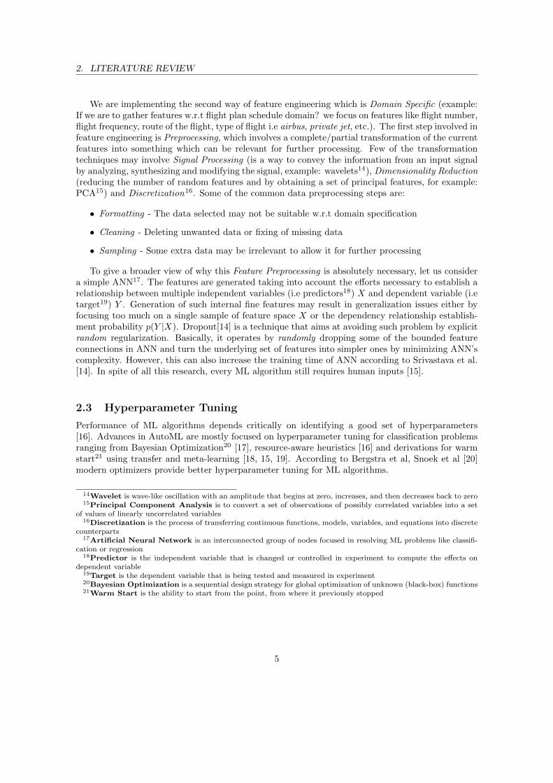
3.1 Random Forests (RF)

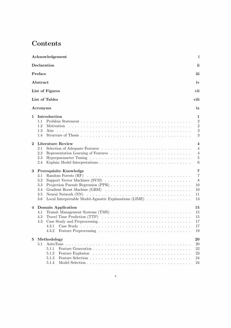
A Decision tree is a flow structure in which each internal node is a test and each branch connectingthe nodes is the outcome of it. The result of the decision tree is represented by the leaf nodes.Decision Tree Learning uses decision tree as a predictive model to map the samples of an item tothe target variable. In a decision tree, the input data is entered at the top of the tree and as ittraverses down, the data gets binned into smaller subsets of the tree [23]. Random Forests workson both classification and regression problems. The specialty of RF is that when creating trees,it generates a small sub-tree by random selection of samples and features (not the complete set).Then the task is repeated until all the samples and features are considered. Finally, an appropriatedecision tree is obtained. For example, say we have 100 samples of 10 features. RF would generatea tree by taking 10 samples and 5 features at random. This process is repeated 10 more times andthen combined together to make a formal informed decision. The figure 3.1 depicts the workingprocess of RF.

Figure 3.1: Illustration of Random Forest Decision Tree Generation [2]

RF run-times22 are quite fast and they are able to deal with unbalanced and missing data. RFwhen used with regression, cannot predict beyond a range in the training data and it may over-fit

22Run-Time is the execution time of the process

3. PREREQUISITE KNOWLEDGE

data sets that are particularly noisy23. Of course, the best test of any algorithm is how well itworks upon a data set. RF combines this with a random selection of samples to train the treeswhich is referred to as bootstrap aggregation or bagging [24]. RF’s hyperparameters are the numberof randomly selected predictors to choose from at each split (mtry) and the number of grown trees(ntree).

3.2 Support Vector Machines (SVM)

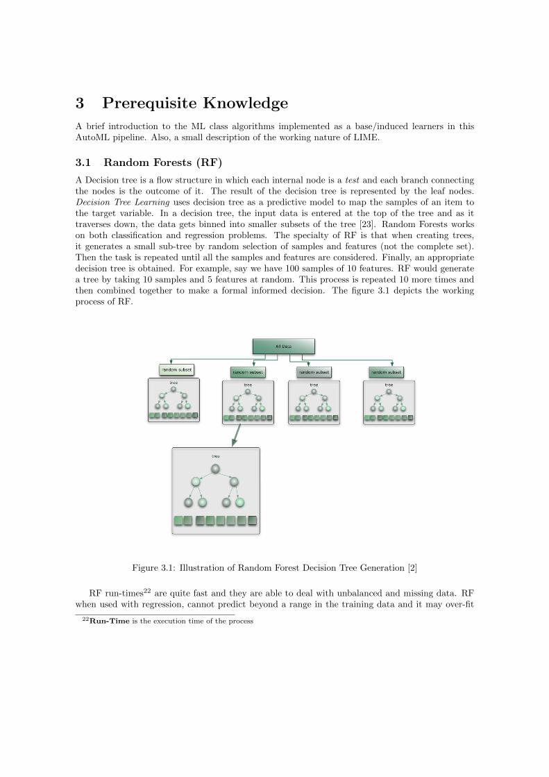
Support Vector Machine was introduced by Cortes et al. in 1995 [25]. They are primarily binaryclassifiers that perform their task by constructing hyperplanes. This is done in a multidimensionalspace where they are able to separate instances either linearly or non-linearly. As shown in thefigure 3.2a, the hyperplane is separating two instance or classes linearly. The closest samples tothe boundary region of the hyperplane (highlighted in figure 3.2a) are called support vectors. Thedistance from the hyperplane to the support vectors (i.e half of the width of the hyperplane) is given

by the measure1

||w||, also known as loss function of errors. The total margin length (i.e the width

of the gray strip as shown in figure 3.2a) is given by measure2

||w||. Minimizing this total width will

maximize the separation of the two represented instances.

(a) SVM with Hyperplane Separation

sni

Slack Variables

(b) Demonstration of Slack Variables in SVM

Figure 3.2: Illustration of SVM classification [3]

Let us assume the width of the hyperplane ranges from [−ε, ε]. The main difference betweenSVM classification and SVM regression comes in the slack variables (as shown in figure 3.2b). SVMfor classification involves assigning one slack variable to each training data point, whereas in SVMfor regression (also labeled as SVR), there are two slack variables for each training data point. Theoptimization function for SVM is given by equation 1 in reference to the figure 3.3a, which illustratesthe slack variables ξn ≥ 0. Data-points with circles around them are support vectors.

C

N∑n=1

ξn +1

2||w||2 (1)

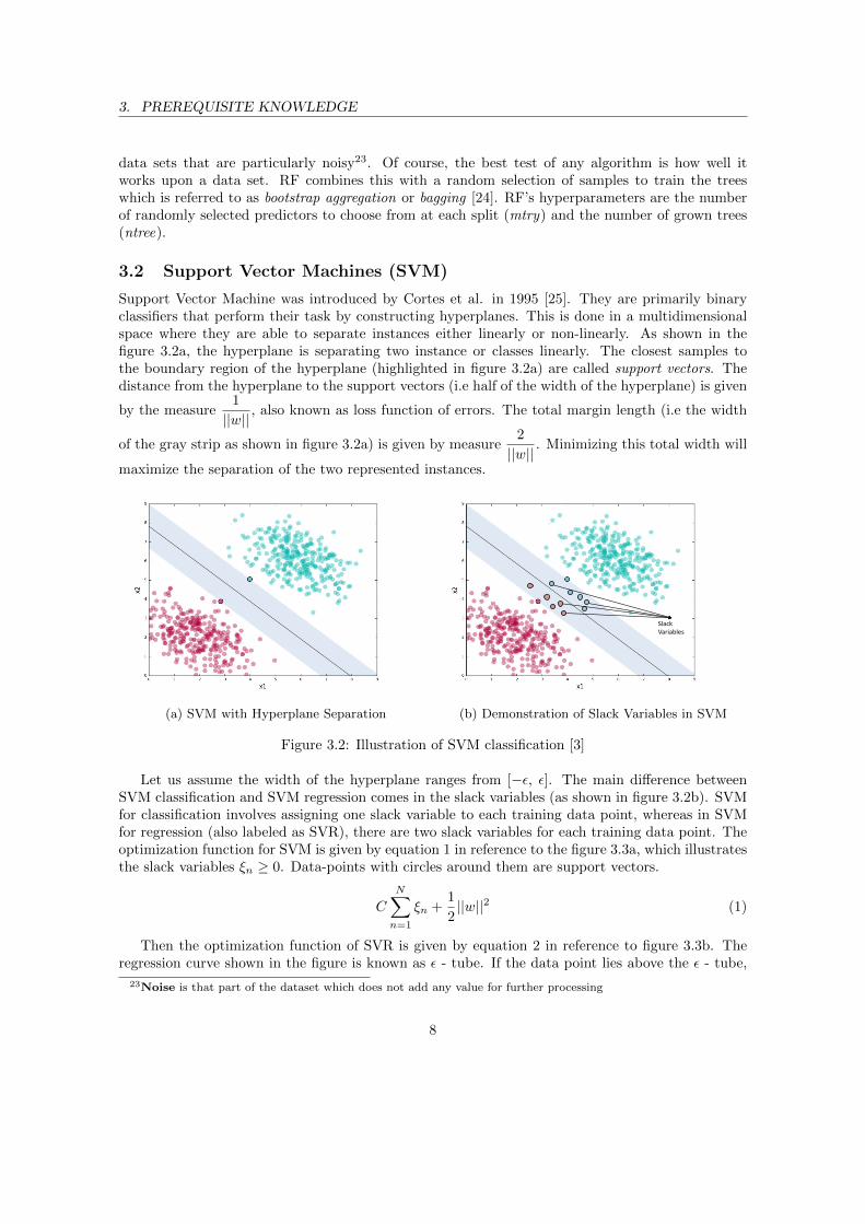
Then the optimization function of SVR is given by equation 2 in reference to figure 3.3b. Theregression curve shown in the figure is known as ε - tube. If the data point lies above the ε - tube,

23Noise is that part of the dataset which does not add any value for further processing

8


we have ξ > 0 and ξ = 0, if the data points are below the ε - tube, we have ξ = 0 and ξ > 0. Datapoints inside the ε - tube, we have ξ = ξ = 0.

C

N∑n=1

(ξn, ξn) +1

2||w||2 (2)

y = 1

y = 0

y = -1

ξ > 1

ξ < 1

ξ =0

(a) Illustration of SVM with Classification

x

y(x) ξ > 0

ξ' > 0

y + ϵ

y - ϵ

y

(b) Illustration of SVM with Regression

Figure 3.3: Illustration of SVM regression

The hyperparameters influencing the respective ML algorithm SVM are: sigma parameter de-fines how far the influence of a single training example reaches, i.e how far the support vectors can bepushed away from the hyperplane. Low values mean ‘far’ and high values mean ‘close’. The sigmaparameters can be seen as the inverse of the radius of influence of samples selected by the modelas support vectors. The C parameter trades off misclassification of training examples against thesimplicity of the decision surface. A low C makes the decision surface smooth, while a high C aimsat classifying all training examples correctly by giving the model freedom to select more samples assupport vectors.

Kernels in SVMs are used to map the data points into higher dimensional feature space (oftenknown as Hilbert space). In such space, the problem turns out to be a linear one. Nevertheless,as the dimensionality of such space can be potentially infinite, SVMs do not consider each sampleprojections, but only the distances between the samples provided by such kernel functions. One of themost common Kernel function is Radial Basis Function (or Gaussian Similarity Kernel Function).The Gaussian Similarity Kernel function is a non-linear function of Euclidean distance given byequation 3.

K(x, y) = exp

(− ||x− y||

2

2σ2

)(3)

The Euclidean distance is given by ||x− y||2. The Kernel function K decreases with distanceand ranges between [0, 1]. Hence, Gaussian Kernel acts as a similarity measure for feature data-points based on the euclidean distance between the data-points. This similarity measure would beconsidered to group the feature data-points to separate dimensions. By doing so, SVM would beable to proceed with the projection of a hyperplane separating this dimensional separation.

9


3.3 Projection Pursuit Regression (PPR)

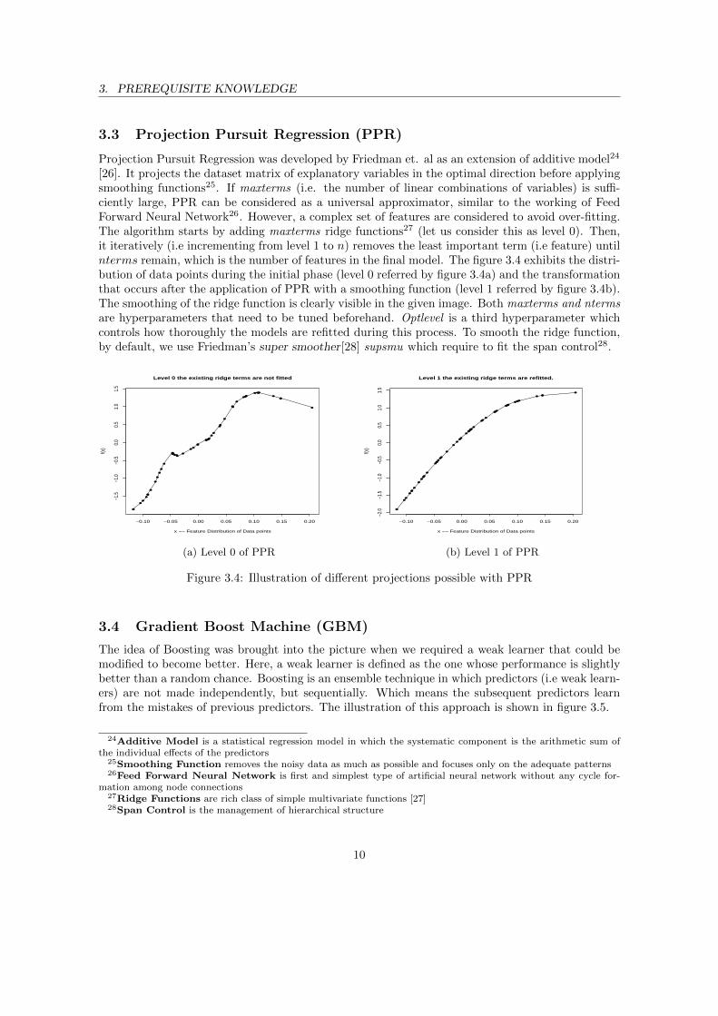
Projection Pursuit Regression was developed by Friedman et. al as an extension of additive model24

[26]. It projects the dataset matrix of explanatory variables in the optimal direction before applyingsmoothing functions25. If maxterms (i.e. the number of linear combinations of variables) is suffi-ciently large, PPR can be considered as a universal approximator, similar to the working of FeedForward Neural Network26. However, a complex set of features are considered to avoid over-fitting.The algorithm starts by adding maxterms ridge functions27 (let us consider this as level 0). Then,it iteratively (i.e incrementing from level 1 to n) removes the least important term (i.e feature) untilnterms remain, which is the number of features in the final model. The figure 3.4 exhibits the distri-bution of data points during the initial phase (level 0 referred by figure 3.4a) and the transformationthat occurs after the application of PPR with a smoothing function (level 1 referred by figure 3.4b).The smoothing of the ridge function is clearly visible in the given image. Both maxterms and ntermsare hyperparameters that need to be tuned beforehand. Optlevel is a third hyperparameter whichcontrols how thoroughly the models are refitted during this process. To smooth the ridge function,by default, we use Friedman’s super smoother[28] supsmu which require to fit the span control28.

●●

●

●

●

●●

●

●

●

●

●

●

●●●

● ●●

●

●●

●●

●●●●

●

●

●

●●

●

●●

●

● ●●

● ●●●

●

●●

●

−0.10 −0.05 0.00 0.05 0.10 0.15 0.20

−1.5

−1.0

−0.5

0.0

0.5

1.0

1.5

Level 0 the existing ridge terms are not fitted

x −− Feature Distribution of Data points

f(x)

(a) Level 0 of PPR

●●

●

●

●

●●

●

●

●

●●

●

●●●

●

●●

●

●

●

●●

●

●●●●

●

●

●●

●

●●●

●●●

●●●

●

●●●

●

−0.10 −0.05 0.00 0.05 0.10 0.15 0.20

−2.0

−1.5

−1.0

−0.5

0.0

0.5

1.0

1.5

Level 1 the existing ridge terms are refitted.

x −− Feature Distribution of Data points

f(x)

(b) Level 1 of PPR

Figure 3.4: Illustration of different projections possible with PPR

3.4 Gradient Boost Machine (GBM)

The idea of Boosting was brought into the picture when we required a weak learner that could bemodified to become better. Here, a weak learner is defined as the one whose performance is slightlybetter than a random chance. Boosting is an ensemble technique in which predictors (i.e weak learn-ers) are not made independently, but sequentially. Which means the subsequent predictors learnfrom the mistakes of previous predictors. The illustration of this approach is shown in figure 3.5.

24Additive Model is a statistical regression model in which the systematic component is the arithmetic sum ofthe individual effects of the predictors

25Smoothing Function removes the noisy data as much as possible and focuses only on the adequate patterns26Feed Forward Neural Network is first and simplest type of artificial neural network without any cycle for-

mation among node connections27Ridge Functions are rich class of simple multivariate functions [27]28Span Control is the management of hierarchical structure

10


Figure 3.5: Illustration of Boosting Sequential Models [4]

Gradient boosting is an example of Boosting algorithm. Gradient boosting involves three ele-ments: a loss function to be optimized, a weak learner to make predictions and an additive modelto add the weak learners to minimize the loss function. Benefit of Gradient Boosting framework isthat a new boosting algorithm does not have to be derived for each loss function used. It is a genericenough framework that any differentiable loss function can be used. Decision trees are used as theweak learner in gradient boosting. Trees are constructed in a greedy manner, choosing the best splitpoints based on purity scores like Gini29 or to minimize the loss. It is common to constrain the weaklearners in a specific way, such as a maximum number of layers, nodes, splits or leaf nodes. Treesare added one at a time, and existing trees in the model are not changed. A gradient descent30

procedure is used to minimize the loss when adding trees. After calculating the loss, to perform thegradient descent procedure, we must add a tree to the model that reduces the loss (i.e. follow thegradient). To do this, we first parameterize the tree. Then modify the parameters of the tree andmove in the right direction by reducing the residual loss. This approach is called functional gradientdescent or gradient descent with functions [29].

After a fixed number of trees are added, the training stops once the loss reaches an acceptablelevel or no longer improves on an external validation dataset. The hyperparameter is tuned to fewsimple basic tree constraints: n.trees is the total number of trees to fit. .interaction.depth is themaximum depth of variable interactions. It implies an additive model (if depth is 2, then it impliesa model with up to 2-way interactions is taken into consideration). n.minobsinnode is the minimumnumber of observations in the trees terminal nodes. shrinkage is a learning rate or step-size reductionmeasure.

3.5 Neural Network (NN)

Neural Network is a computational model that is inspired by the way biological neural networksin the human brain process information. The basic unit of computation in a neural network is theneuron, often called a node or a unit. It receives input from other nodes, or from an external sourceand computes an output. Each input has an associated weight (w), which is assigned on the basis

29Gini Index is a measure of how much the distribution is stretched or squeezed30Gradient descent is a first-order iterative optimization algorithm for finding the minimum of a function

11


of it’s relative importance to other inputs. The node applies a function f (defined below) to theweighted sum of its inputs as shown in figure 3.6.

Figure 3.6: Representation of Basic Neuron with it’s Input and Output [5]

The output Y from the neuron is computed as shown in figure 3.6. The function f is a non-linear function and is called the Activation Function. The purpose of the activation function is tointroduce non-linearity into the output of the neuron. This is important because the real world datais non-linear and our intention is to learn these non-linear representations.

Training the input vectors in perceptron is achieved by presenting the data to it one after another.Weights are modified according to the equation 4. For all inputs i,

W (i) = W (i) + α× (T −A)× P (i) (4)

Here, W is the weight vector, P is the input vector, T is the correct output that the perceptronshould have known and A is the output of the given perceptron. Certain limitations of using theperceptron is that, if the input vectors are not linearly separable, learning will never reach a pointwhere all vectors are classified properly. We intend to use Multilayer Perceptron (MLP). It is asimple basic Neural Network, where the perceptron is divided into 3 layers: input, middle and outputlayers (refer to figure 3.7). The number of neurons or nodes in each layer will be our hyperparameterto tune. They are represented as layer1, layer2 and layer3 respectively.

12

INPUT LAYER MIDDLE LAYER OUTPUT LAYER

Figure 3.7: Illustration Multilayer Perceptron

3.6 Local Interpretable Model-Agnostic Explanations (LIME)

Machine Learning ML is one of the most recognized buzzwords. With computers like IBM Watsonwinning jeopardy, one tends to wonder, if the system can be a better driver or a doctor. ManySoA ML model is a black box. The internal working of the model is impossible to understand andcontrol. This brings the question of trust. How well can one trust the ML model and its predictions,without knowing its interpretations?

Gaining better explanation behind individual predictions would put us in a better position totrust or mistrust the model. Even if we cannot necessarily understand how the model behaves inall cases, it may be possible to understand how it behaves in particular cases. One can alwaysargue that if the learning model gives a good accuracy, the system is performing at its peak. But,the accuracy of cross-validation can be very misleading [30]. Sometimes data that should not beavailable, leaks into the training data accidentally. Also, the way the data is gathered may introducecorrelations. Many such problems would give us a false understanding of the performance.

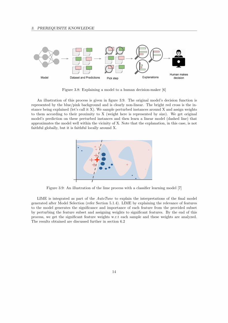
Local refers to local fidelity, i.e. we want the explanation to really reflect the behavior of theclassifier/regressor around the instance being predicted [7]. Some Learning models use representa-tions that are not intuitive to users at all. LIME explains those representations in terms, a user canunderstand. LIME is able to explain any model without peeking into it, hence it is model-agnostic.To figure out which parts of interpretable input (i.e features) are contributing to the prediction, theneighbours of the input are perturbed and then the model’s prediction behavior is checked. Thenthese perturbed data points are assigned weights by their proximity to the original sample. Forexample, if we are trying to explain the prediction for the sentence ”I love this burger”, LIME willperturb the sentence and get predictions on sentences such as ”I love burger”, ”I this burger”, ”Iburger”, ”I love”, etc. The described pick step is exhibited in figure 3.8. If the original classifier/re-gressor takes many more words into account globally, it is reasonable to expect that around thisexample only the word ”love” will be relevant.


Figure 3.8: Explaining a model to a human decision-maker [6]

An illustration of this process is given in figure 3.9. The original model’s decision function isrepresented by the blue/pink background and is clearly non-linear. The bright red cross is the in-stance being explained (let’s call it X). We sample perturbed instances around X and assign weightsto them according to their proximity to X (weight here is represented by size). We get originalmodel’s prediction on these perturbed instances and then learn a linear model (dashed line) thatapproximates the model well within the vicinity of X. Note that the explanation, in this case, is notfaithful globally, but it is faithful locally around X.

Figure 3.9: An illustration of the lime process with a classifier learning model [7]

LIME is integrated as part of the AutoTune to explain the interpretations of the final modelgenerated after Model Selection (refer Section 5.1.4). LIME by explaining the relevance of featuresto the model generates the significance and importance of each feature from the provided subsetby perturbing the feature subset and assigning weights to significant features. By the end of thisprocess, we get the significant feature weights w.r.t each sample and these weights are analyzed.The results obtained are discussed further in section 6.2

14

4 Domain Application

An introduction to the Domain of the system and the major problem associated with it. Case studyof the type of data which can be extracted from the system and also the preprocessing techniquesrequired, which would help in resolving the problem faced by the domain system.

4.1 Transit Management Systems (TMS)

Transit Management System[31] is referred to as an Intelligent Infrastructure which establishes cer-tain guidelines for a continuous and smooth flow of day to day transportation services. TMS alsoprovide us with real-time data on these services. Real-time data can be collected from varioussources: hand-held devices like Smart-Phones, wearable devices like Smart-Watches, Heart-Ratemonitor and integrated devices like GPS31 (Global Positioning System) in a car. These devices areembedded with sensors to transfer data in wireless32 mode. Some of the other devices are GSM33,(Global System for Mobile Communications), 3G34, GPS, and WiFi35. With advancements in theabove-mentioned devices, gathering data has never been easier. Collecting these datasets has itsimportance to many big companies. They need this collected information to perform certain taskssuch as analysis and developing their business intelligence and marketing strategies. Planning fi-nancial and resource management are some of the other crucial tasks performed with this collectedinformation. Public Transportation (PT) is one such domain, which offers a good showcase of thistrend. It is a highly competitive domain, where the analysis of real-time data could potentially leadto service improvements and ultimately increase their market value. In the last decade, TMS hasbeen deployed in many PT companies and the Automatic Vehicle Location (AVL)36 data collectedby these systems are later used for off-line evaluation of service performance and reliability.

4.2 Travel Time Prediction (TTP)

Countries like Japan [32] (railway service provided by Japan Railway Group) and Germany [33](Deutsche Bahn railway services provided by German Railway Company) are subjected to largepenalty if certain standards of services are not met. A lot of guidelines and conditions are imposedto maintain the quality of transportation services. Hence, predicting arrival time of the transportcan be a favoring factor to maintain this quality of service. To maintain quality, certain performancemeasures such as On-Time Performance37 (OTP) and Excessive Waiting Time38 (EWT) need to beoptimized. There are a lot of varying factors which can affect the prediction of an arrival time. Iden-tifying these varying factors that affect Travel Time (especially during stops/schedule time points)is termed as Travel Time Prediction problem (TTP).

One can clearly distinguish between short-term and long-term travel time prediction problembased on the Prediction Horizon (example: threshold of 1 hour is a short-term TTP, where as long-

31GPS is a satellite-based radio navigation system that provides geo-location and time information32Wireless is a mode for transferring data without hard physical connections33GSM is a standard developed by the European Telecommunications Standards Institute (ETSI) to describe the

protocols for second-generation digital cellular networks used by a mobile device343G is the third generation of wireless mobile telecommunications technology35WiFi is a technology for wireless local area network with devices based on the IEEE 802.11 standards36Automatic Vehicle Location is a mobile and wireless system, embedded in vehicles which constantly collects

information like current global position (latitude and longitude), bus stop ID, driver ID etc.37On-time Performance is a measure of the ability of transport services to be on time38Excessive Waiting Time is the maximum possible time to wait for the transport services to arrive

4. DOMAIN APPLICATION

term TTP is assumed over a period of 1 month or more). Operational tasks (example: timetabledesign) or resource allocation (example: vehicle and crew scheduling) requires long-term TTP. Atraditional approach to TTP is Regression Analysis39. The end result is to estimate the relation-ship between a set of independent variables and a dependent variable. Equation 5 exhibits thisrelationship.

f : xi, θ ⇒ R such that f(x, θ) = f(xi) = yi,∀xi ∈ X, yi ∈ Y (5)

where f(xi) denotes the true unknown function which is generating the samples’ target variable

and f(xi; θ) = yi be an approximation dependent on the feature vector xi and an unknown (hyper)parameter vector θ ∈ Rn (given by some induction model M). This approximation gives us theimportance of hyperparameter values referred by M to the dependence structure of f as well asthe relevancy of the input feature space X. If it has a low number of features, it may not explainthe variance40 of Y , thus leading M to be a biased41 model (under-fitting). Conversely, for a largeset of features, we can use features with a low predictive power. In consequence, M may outputhigh complex models which leads to optimal fit on the input dataset (over-fitting). Achieving thistrade-off between the bias and variance is the key to identifying the hyperparameters responsible toboost the identification and utilization of those relevant feature space42.

A long range of methods are employed to resolve TTP problems from different research areas[34]. These can be folded into four categories:

• ML and regression methods [35, 36]

• State-based and time series models [37]

• Traffic Theory-based models [38]

• Historical data based models [39, 40]

The first two approaches return models with high predictive power and low explanatory aspects[31]. The other two approaches are inverse to the first two approaches and therefore not consideredin this report. State-based and time series works best in predicting short-term TTP problems [31].Short-term TTP is related to real-time information of the arrival time which is provided by Auto-matic Traveler Information System (ATIS)43[41]. The position and surpassed time of each vehicleis forwarded to the server to update its predictable forecasts. This update and predict way of learn-ing is known as Adaptive Learning, which provides better results for short-term TTP. However,this can be employed on off-line regression models with Hybrid type models that integrate KalmanFilter 44. Wall et. al [42] suggests that in this approach linear regression models handle TTPand Kalman Filter exacts position and predicts arrival time. Moriera-Matias et. al [43, 44] high-lights the drawbacks of using parametric approaches45 (the model trained by parametric approach

39Regression Analysis is a set of statistical processes for estimating the relationships between independent vari-ables and a dependent variable in ML technique

40Variance is an error from sensitivity to small fluctuations in the training dataset41Bias is an error from erroneous assumptions in learning algorithm42Relevant Feature Space is a feature space composed of only relevant features43Automatic Traveler Information System is a system where trip plans can be automatically generated based

on the active transit network and real-time service schedule at the time of travel44Kalman Filter uses a series of measurements observed over time and estimate unknown variables that tend to

be more accurate than those based on a single measurement alone45Parametric Approach assumes that there are fixed set of parameters that determine a probability model

16

would not adapt to new changes). We propose a stochastic approach where a model is generatedbased on random variables instead of predefined ones. This approach is non-parametric46 as it candeal with changes in the residual distribution functional form without drawing assumptions about it.

Some of the main determinants to be collected via the real-time data47 are route length, pas-senger activity at stops and the number of traffic signals [45, 46]. Other studies also added driverresponse to the deviation from the schedule as an explanatory feature [47, 48]. However, all of thesefactors are estimated by linear regression48 models to identify the impact of potential explanatoryvariables on bus running times. Consequently, the resulting models often have very limited predic-tive power. Some of the other deciding factors would be travel times, scheduled times and holidaysin the state or the country under consideration. Sometimes the total population covered in thespecific area makes a lot of difference and also peoples’ preferred mode of transportation (public orprivate means) also matters.

Some of the main concerns involved with TTP are passenger induced delays (example: vehiclebreak-down and operator’s unavailability). The determinants in the above-mentioned paragraphcan give rise to a non-linear model49. The complexity of the non-linear model is even higher ascompared to a linear model50. The literature to handle this specific issue is scarce. RReliefF [49]was proposed to do an adequate feature selection. This is a well-known approach. Some of the othermethods which are part of RReliefF family are an instance-based learning51 method. This leveragesthe concept of the neighborhood to define features that can (or cannot) contribute to estimatingthe target variable Y . One of the drawbacks of instance-based learning is redundant features. Aprior research of NLE [50] demonstrated that the Least Absolute Shrinkage and Selection Operator(LASSO) method can easily outperform RReliefF to resolve TTP. More details about LASSO isgiven in section 5.2.1.

Long-term TTP is known as off-line regression problem [35, 51]. A meta-learning approachAutoTune, as instructed in section 5.1, combines base learners like Support Vector Machines (referto section 3.2), Project Pursuit Regression (refer to section 3.3), Random Forest (refer to section3.1), Gradient Boost Machine (refer to section 3.4) and Neural Networks (refer to section 3.5) toresolve the respective problem.

4.3 Case Study and Preprocessing

4.3.1 Case Study

Our case study is a large urban bus operator in Stockholm, Sweden. The proprietary data werecollected on four high-frequency routes A1/A2/B1/B2, i.e. two bus lines A/B, between 07:00 and19:00 hrs. Line A connects residential areas to a public transport interchange hub covering some ofthe major shopping areas. B connects the southern parts of the city to the center of the city, passingthrough an interchange, major hospitals, and a possible logistic center. The study duration as noted

46Non-parametric Approach is a set of parameters that determine probability model is not fixed47Real-Time data is the information that is delivered immediately after collection48Linear Regression line has an equation of the form Y = a + bX, where X is the explanatory variable and Y is

the dependent variable49Non-Linear Model is a model with equation that can attain multiple forms with changing variables50Linear Model is a model with equation having only one linear form51Instance-Based Learning is a family of learning algorithms, which tries to predict by comparing new instances

with observed instances in the training set


covers six months between August 2011 and January 2013. The study period starts from winterschedule and goes on till summer schedule. These 6 months of data were collected between the years2011-2013. The Figure plots 4.1a and 4.1b exhibit’s the roadmap followed by the above-mentionedbus lines and also the intermediate stops the bus lines take.

(a) Stocholm Bus Line A Route (b) Stocholm Bus Line B Route

Figure 4.1: Stockholm Bus line A/B Route Map

Table 4.1, gives a breakdown of each fields and field types associated with the raw data. Thedata is collected and stored in a CSV file, which is later considered as input in the experimentsection. The data contains several static and dynamic attributes of the bus. Among the dynamicattributes are real-arrival time, real-departure time, number of boarding, number of alighting etc.Some of the static attributes are vehicle-id, scheduled departure time, scheduled arrival time, stop-id,scheduled-roundtrip time etc.

Field Name Description Field Type

utrip id1 Trip Identifier Factorvid1 The Vehicle Identification Number Numericalldates1 The date of the recorded data associated to the bus and

the tripDate

sched time1 The Scheduled departure time of the bus from each stop Timestampsched rtt1 The Scheduled Round trip time in seconds for the bus to

complete it’s entire route and reach back to the startingpoint

Numeric

dep stop name1 The Initial Starting Point stop name Stringdep stop id1 The Initial Starting Point stop Id Numericstop name1 The Stop Name at which the bus stops Stringstop id1 The Stop ID at which the bus stops Numericsched arr time1 The scheduled arrival time of the bus at each stop Timestampr arr1 The actual arrival time of the bus at each stop Timestampsched dep time1 The scheduled departure time of the bus from each stop Timestampr dep1 The actual departure time of the bus from each stop Timestamp

Table 4.1: Field, Description and Field-Type of Stockholm collected data

18


4.3.2 Feature Preprocessing

Just gathering the data is not enough. We need to evaluate each field and identify those fea-tures/fields which could serve our purpose. The remaining features/fields not considered for furtherprocessing are labeled as noise or irrelevant features. The focus lies on identifying the types ofrequired features. We are mainly concerned with categorical type, time type, date type and numerictype fields. This preprocessing step would automatically identify the type of field and filter out therequired types as the relevant features.

The preprocessing step also splits the entire dataset in terms of trip-id to compute the realround-trip time in accordance with the real-departure time and real-arrival time. The new fieldgenerated would be the associated target variable. Also, we need a categorical value based on whichwe can cluster the entire data based dimensionality check, which will be briefly explained in section5.1.1. The time and date types would be additional supporting features. The original features aredeparture time (i.e. a Julian timestamp) and vehicle ID (i.e. categorical referred to as veh id).

Let the history of a given route with n stops be defined by S trips of interest. Let trip i of agiven bus route be defined by Ti = {T 2

i , T3i , ..., T

ni } where T ji stands for the travel time between

bus stops j and 1 at trip i (i.e. the time elapsed between the departure time at bus stop 1 andthe departure time at bus stop j of the vehicle running the trip i). Let X be a multidimensionalfeature space where X ∈ RN : ‖X‖ ≤ 1 while Y ∈ R+ denotes a target (example: the travel timeT 2i ). Let the dependence relationship between Y and X be explained by a function f . Our goal

is to discover/approximate such function f using the above mentioned S input trips. By adaptingequation 5, we can do it by:

f : xi, θ, α⇒ R+suchthatf(x, θ) = f(xi) = yi,∀xi ∈ X, yi ∈ Y (6)

where θ denotes a vector of model parameters while α stands for a series of hyperparametersthat may vary along the selected induction learner (i.e. the algorithm that we choose/device to inferf and θ from the initial S samples).

After identifying the relevant features from the raw-feature, create a hierarchical structure ofthe current feature set (example: Time feature is broken down into minutes, hours and seconds).Similarly, we implement multiple ways of breaking down the current feature set to atomic leveldepending on their types and maybe generate a combination of features.

19

5 Methodology

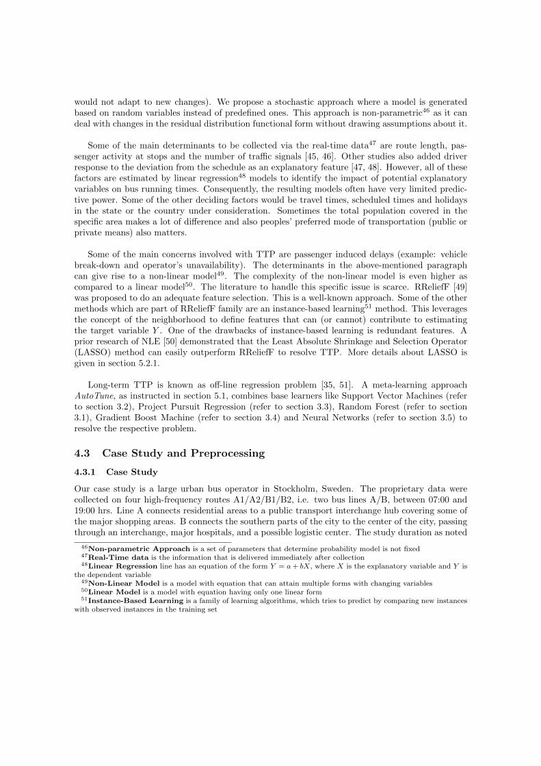
5.1 AutoTune

PREPROCESSING

Model 1

Auto ML Ensemble Learning

Model 2

SRL Model 3

Model N

Drift Detection

BL stands for Base Learner and it can represent a model learned by an ML paradigm. Example SVMs, RFs, ANNs etc.

BL 3

SRL BL N

SRL BL 1

SRL BL 2 Interpretable

Feature Hierarchies

Accurate Predictions

Explanatory Visual Analytics

Output Input (Data Sources)

Database

Internet

time

Figure 5.1: General Illustration of AutoTune pipeline

AutoML pipeline AutoTune [15] developed by NLE, was earlier introduced in Chapter 1. AutoTuneis regulated by five principles:

• Automation - AutoTune removes the human interference by approximating suitable datarepresentations and model hyperparameter tuning

• Versatility - AutoTune relies on learning Multiple Explanatory Models with distinct learningalgorithms. On the top, AutoTune encloses a unique Meta-Learning approach enabling it tolearn which is the best model (combination) to address each query at every instance

• Interpretability - AutoTune representations are user interpretable. It is learned based onFeature Hierarchies, allowing the learned features to map to the original/raw features. Conse-quently, this process implements Shallow Representation Learning (SRL) described below

• Practicability - AutoTune can learn continuously. Consequently, it is able to make predic-tions both on-demand and in real-time

5. METHODOLOGY

• Adaptiveness - AutoTune can cope with changes in the underlying distribution and contin-uously generate reliable models and predictions under any scenario irrespective of any uncer-tainty

An illustration on AutoTune is introduced in figure 5.1. Drift detection in the this figure is todetect unforeseen changes in the model that may occur in the statistical properties of the targetvariables, which the model is trying to predict.

Shallow Representation Learning (SRL) is a stepwise Representation Learning (refer to section2.2) engine which can be coupled with many available ML algorithms (example: Support VectorMachine (refer to section 3.2), Random Forest (refer to section 3.1) etc. Each dataset comes withits own anomalies in an explanatory model (example: if the dataset is to resolve TTP, the vehicletaken may pass through narrow roads and the vehicle type used in such services may have a largeinfluence on the travel time experienced in that route). The main objective of SRL here is to solvethe problem of finding appropriate relevant feature subset by hyperparameter tuning, that mini-mizes generalization error induced by machine learning algorithms. Also, depending on the typeof induced learners, the subset of features may need to exhibit certain representation which makeslearners perform to the best of their abilities. SRL encloses an advanced combination of automatedfeature engineering techniques. They can be supervised and unsupervised feature selection methods,as well as user-defined filters and wrappers. Which aims to achieve near-optimal trade-offs betweenreduction of inductive bias error and increase of variance error. These characteristics are responsiblefor maximizing the predictive power of any TTP algorithm by providing a generalization error nearto it’s global optimum and a highly accurate long-term ETA in an automated implementation.

The role of SRL is elaborated in AutoTune-SRL (refer to section 5.2.2). The main idea is tofind an adequate feature subset which can be forwarded to the base learners. It starts with thenovel concept of Feature Explosion (refer to section 5.1.2), where we map the initial raw featuresinto a higher and sparse multidimensional space by applying different types of feature engineeringtechniques (refer to section 5.1.1). These transformations could be considered as Hierarchical rep-resentation of original/raw features. These hierarchical features aim to identify contexts of featuresthat may be relevant for TTP (example: late afternoon services performed by vehicles), which maynot be sufficiently explicit in the original representation. The second stage SRL is a five-step filter-type feature selection procedure that aims to reduce this sparse space with a smaller one, where allfeatures of the smaller subset are somehow relevant to resolving the TTP. Finally, a combinatorialoptimization technique called as BAM (inspired by Sequential Backwards Floating Feature Selec-tion from Somol et al. [52]) is devised to select the optimal feature subset as well as an optimalhyperparameter tuning to employ with a given dataset/route and induction learner (refer to section5.2.2.5).

Experiments were conducted using a large-scale AVL dataset collected from a mass transit agencyoperating in Stockholm, Sweden. The obtained results showed that AutoTune outperforms the SoA(refer to section 5.2.1) by almost 32% which can be seen in section 6.2.

This section gives us a breakdown of individual steps involved in setting up the AutoTune frame-work. The methodology can be broken down into six steps as given below and illustration of thebelow steps are represented in figure 5.2 :

• Feature Generation - A tailor-made procedure which involves generation of a hierarchy offeatures from the original dataset required by supervised ML techniques (refer to section 5.1.1)

21

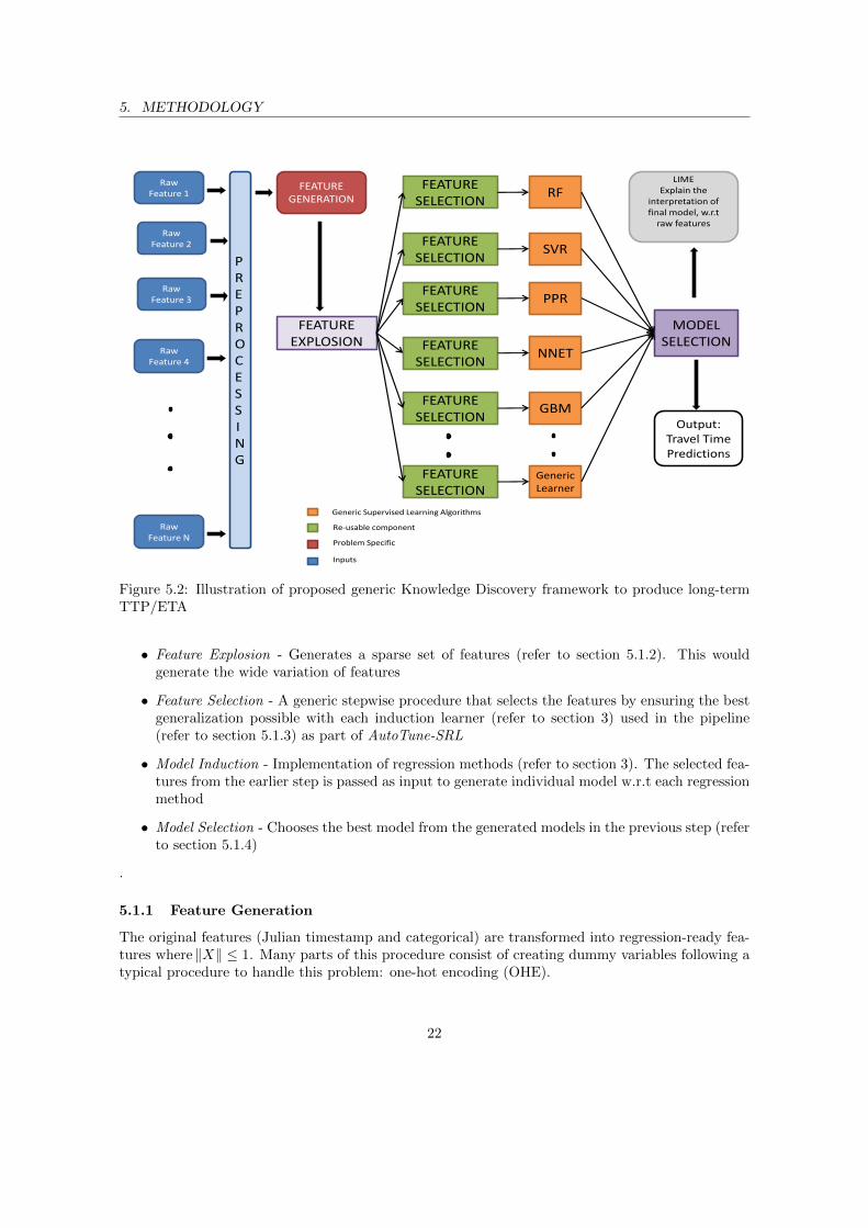
5. METHODOLOGY

Raw Feature 1

PREPROCESSING

FEATURE GENERATION

FEATURE SELECTION

RF

MODEL SELECTION

FEATURE EXPLOSION

FEATURE SELECTION

SVR

FEATURE SELECTION

PPR

FEATURE SELECTION

NNET

FEATURE SELECTION

GBM

FEATURE SELECTION

Generic Learner

Raw Feature 2

Raw Feature N

Raw Feature 3

Raw Feature 4

Output: Travel Time Predictions

Generic Supervised Learning Algorithms

Re-usable component

Problem Specific

Inputs

LIME Explain the

interpretation of final model, w.r.t

raw features

Figure 5.2: Illustration of proposed generic Knowledge Discovery framework to produce long-termTTP/ETA

• Feature Explosion - Generates a sparse set of features (refer to section 5.1.2). This wouldgenerate the wide variation of features

• Feature Selection - A generic stepwise procedure that selects the features by ensuring the bestgeneralization possible with each induction learner (refer to section 3) used in the pipeline(refer to section 5.1.3) as part of AutoTune-SRL

• Model Induction - Implementation of regression methods (refer to section 3). The selected fea-tures from the earlier step is passed as input to generate individual model w.r.t each regressionmethod

• Model Selection - Chooses the best model from the generated models in the previous step (referto section 5.1.4)

.

5.1.1 Feature Generation

The original features (Julian timestamp and categorical) are transformed into regression-ready fea-tures where ‖X‖ ≤ 1. Many parts of this procedure consist of creating dummy variables following atypical procedure to handle this problem: one-hot encoding (OHE).

22

5. METHODOLOGY

The Julian timestamp with respect to the departure time is split into two base features: timeand day. The time features are further folded into 2 more features namely hours and minutes. Thehours are encoded into hourly bins resulting in a total of 24 features and the minutes are encodedinto 4 features of 15-minutes folds, grouping the minutes into each quarter bin in an hour. The daysare encoded in different types of bins with respect to the week in a year bins of 52 features, monthlybins of 12 features and weekday of 7 features. Also, the hours are encoded, implementing equalfrequency discretization52 which gives an additional 10 features (10 bins). Additional binary flagsdenoting holidays and Winter/Summer season of 2 features are considered. Finally, two variablesare combined to generate 6 features of binary values, AM peaks/PM peaks/Off-peaks with respectto working days and weekends. This sums up to 119 time-dependent features.

Vehicle Ids (categorical feature) undergoes High-Dimensionality Check. If the number of uniqueVehicle Ids ≥ 0.1% of the total number of samples, then we check if there are individual categoriescovering at least 20% of the total number of samples. If true on both the checks mentioned above,then the data can be clustered. If not, then it is encoded implementing equal frequency discretiza-tion which would give up to 10 features (10 bins). We consider a 3-step clustering procedure. First,Kernel Density Estimation (KDE) is used to generate the Probability Density Function (p.d.f)53 forevery unique vehicle id. Second, this p.d.f was clustered by a Gaussian Mixture Model [53] trainedusing the Expectation-Maximization algorithm. Finally, the Bayesian Information Criterion54 (BIC)was used to select the best model. This procedure results in a four-fold categorical variable of 5features. Starting with generation of 21 features, this is done by selecting equally spaced pointsfrom the KDE and used as numerical features, this creates twenty-one equally spaced clusters withrespect to the entire dataset. In the second fold, 6 features from cluster-based descriptive statisticsare generated with respect to their travel times: mean, median, standard deviation, maximum andminimum. In the third fold, we again compute equally spaced twenty-one density points by clus-tering the distribution of vehicle id, giving rise to 21 more features. Finally, a single binary featureindicating if the sample is an outlier55 (not part of any cluster) is also considered. This sums up to54 vehicle-dependent features.

The irrelevant features are removed from the modified dataset and this results in 136 features.This could be the first stage of hierarchical feature set originated from the original raw features.These features are normalized i.e scaling between ∈ [0, 1] in 4 steps: subtract their mean, dividethem by their standard deviation, subtract their minimum value and divide them by their maximum.

5.1.2 Feature Explosion

Algebraically, we can define a dot product between two features i and j as follows:

xi · xj =

S∑k=1

xi,kxj,k (7)

Two vectors are independent when their dot product is null, indicating they are orthogonal. Weexploited this concept in this context of feature generation by generating a pool of new features

52Equal Frequency Discretization method ensures that each bin contains approximately the same number ofsamples

53Probability Density Function is a function of a continuous random variable, whose interval gives the proba-bility that the value of the variable lies within the same interval

54Bayesian Information Criterion is a criterion for model selection among a finite set of models55Outlier are variables that are not part of the context

23

to add to the original ones by leveraging on the dot product coefficients (i.e. multiplication of thefeatures for each sample). By doing so, we are giving the base learners the possibility of exploringexplicit concepts (example: vehicle experience delays during winter for specific route and time). Theresultant data-set is the second stage collection of wide range of hierarchical feature set.

5.1.3 Feature Selection

Feature selection is the process of selecting a subset of relevant features (variables, predictors) totrain a model. Feature selection techniques are used mainly for four reasons:

1. Simplification of models to make them easier to interpret

2. To avoid the dimensionality issues

3. Enhance generalization by reducing over-fitting (reduction of variance)

4. Reduce the training time

Feature selection techniques are completely different from feature extraction. Feature extractioncreates new features from functions of the original features, whereas feature selection returns a sub-set of the features. Feature selection techniques are used at times when there are many features andcomparatively fewer samples. Some of the scenarios where feature selection is applicable include theanalysis of written texts and DNA micro-array data, where there are thousands of features for onlya few samples.

We consider two feature selection techniques. One of the technique is well known and widely usedfor selection of features i.e LASSO (refer to section 5.2.1). The other is NLE developed AutoTune-SRL (refer to section 5.2.2). Section 5.2 compares both the techniques in terms of how adequate orimportant the features are in the generation of an adequate model. The end result of these imposedtechniques is a subset of features, which is considered as relevant by the underlying learned model.

5.1.4 Model Selection

An ensemble procedure Bucket of models [54], an hold-out validation set is kept to estimate the lossof each computed model. This procedure can be done once or multiple times for different validationsets. The advantage is that the procedure does not involve any further tuning. The drawback isthat output model is never better than any of the ones already put in the pool.

5.1.5 Postprocessing

The final set of features/hyperparameters obtained and the errors generated by severe outliers inp(y) are handled. This is accomplished by evaluation of generalization errors in different scenarios.Generalization error is evaluated by considering the below scenarios w.r.t each induced learner (referto section 3).

• Log-transformation of the target - turns the target distribution close to a Gaussian

• Removing outliers according to Tukey definition [55]

• Combination of the above approaches

Now we have five specific models. One from section 5.1.4, and four distinguishable models fromthe current section.

5. METHODOLOGY

5.2 Feature Selection Techniques

5.2.1 LASSO - baseline for Feature Selection

LASSO is a shrinkage and selection method for a linear regression introduced by Tibshirani [56].Similar to other shrinkage methods (example: Ridge Regression), it aims to improve the least-squaresestimator by adding constraints on the value of coefficients. Given N vectors of size n, where Nis the number of samples and n is the number of features and an outcome y, LASSO fits a linearregression model where the parameter estimates are given in Equation 8:

blasso = argminb

1

2

N∑i=1

(yi − b0 −n∑j=1

xi,j × bj)2 +λ

2×

n∑j=1

|bj |2 (8)

The L1− norm penalty of LASSO approach allows a stronger constraint on the coefficients andcauses some coefficients to be shrunk exactly to zero. The tuning parameter λ controls the strengthof the penalty. As it increases, more coefficients are set to zero and hence, fewer variables are se-lected. It is typically set by using a cross-validation search technique over a grid of admissible values.

The zero-valued coefficients of LASSO can be used to remove irrelevant features as mentionedin an earlier NLE research paper [50]. The resultant feature space can then be used with anyavailable base learner, independently on its assumptions with respect to the functional form (i.e.linear/non-linear) of the underlying explanatory model.

5.2.2 AutoTune-SRL

AutoTune-SRL - a generic procedure to learn interpretable representations that are suitable to han-dle the bias-variance trade-off, necessary to find adequate generalizations throughout the supervisedlearning pipelines. It was already introduced in section 5.1. In this section, we will go step by stepin understanding the entire process involved.

AutoTune-SRL settles on seven sequential steps as displayed in figure 5.3. Unlike many otherstandalone feature selection frameworks, AutoTune-SRL operates as an optimization frameworkthat aims to find the best possible representation (i.e. features) for a given pair of dataset andbase learner. It takes into account the removal of redundant and irrelevant features while keepingthe ones that guarantee the best possible trade-off between inductive bias/variance. The intuitionbehind its definition is to generate a near infinite pool of possibilities. This is then pruned downin a very specific way towards keeping an optimal representation of our concepts. This is not onlydriven by data but also by the different assumptions that every learner makes on the underlyingdependence structure. The steps of this framework are now formally described in figure 5.3

25

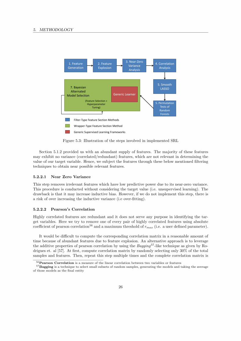
5. METHODOLOGY

1. Feature Generation

4. Correlation Analysis

3. Near-Zero Variance Analysis

2. Feature Explosion

5. Smooth LASSO

5. Permutation Tests of Random Forests

Generic Learner

7. Bayesian Alternated

Model Selection

(Feature Selection + Hyperparameter

Tuning)

Filter-Type Feature Section Methods

Wrapper-Type Feature Section Method

Generic Supervised Learning Frameworks

Figure 5.3: Illustration of the steps involved in implemented SRL

Section 5.1.2 provided us with an abundant supply of features. The majority of these featuresmay exhibit no variance (correlated/redundant) features, which are not relevant in determining thevalue of our target variable. Hence, we subject the features through these below mentioned filteringtechniques to obtain near possible relevant features.

5.2.2.1 Near Zero Variance

This step removes irrelevant features which have low predictive power due to its near-zero variance.This procedure is conducted without considering the target value (i.e. unsupervised learning). Thedrawback is that it may increase inductive bias. However, if we do not implement this step, there isa risk of over increasing the inductive variance (i.e over-fitting).

5.2.2.2 Pearson’s Correlation

Highly correlated features are redundant and it does not serve any purpose in identifying the tar-get variables. Here we try to remove one of every pair of highly correlated features using absolutecoefficient of pearson correlation56 and a maximum threshold of rmax (i.e. a user defined parameter).

It would be difficult to compute the corresponding correlation matrix in a reasonable amount oftime because of abundant features due to feature explosion. An alternative approach is to leveragethe additive properties of pearson correlation by using the Bagging57-like technique as given by Ro-drigues et. al [57]. At first, compute correlation matrix by randomly selecting only 30% of the totalsamples and features. Then, repeat this step multiple times and the complete correlation matrix is

56Pearson Correlation is a measure of the linear correlation between two variables or features57Bagging is a technique to select small subsets of random samples, generating the models and taking the average

of those models as the final entity

26

5. METHODOLOGY

obtained by averaging the outputs of all the possible iterations.

5.2.2.3 Smooth LASSO

The LASSO method is already mentioned in Section 5.2.1. The purpose here is to remove the ir-relevant features. We leverage on the expressiveness of the LASSO curve to prune out irrelevantfeatures [50]. We apply the smooth version of LASSO, which considers only a percentage of theoptimal regularization parameter value denoted by 0 ≤ x ≤ 1 (i.e. a user-defined parameter).

5.2.2.4 Permutation Tests of Random Forests

This is another supervised feature selection technique by assessing the predictive power of eachfeature, similar to Near Zero Variance as explained in section 5.2.2.1 is the other one). The currentfilter method is known as Permutation Importance or Mean Increasing Error (MIE) - commonlyused in Random Forest (refer to section 3.1). MIE assigns a score to each feature by baggingtechnique, removing a feature and evaluating its impact on predicting the target. The breakdownof this process is as given:

1. The error of each tree is assessed using the out-of-bag58 data (the data that was not part ofthe bootstrap used to build the tree)

2. The same procedure is applied to each feature of the tree

3. The differences of each pair (feature j, tree i), i.e. vi,j , can be used to compute MIE withequations 9 and 10

µMIEj=

1

ρ

ρ∑i=1

vi,j ;σMIE =

√√√√1

ρ

ρ∑i=1

(vi − µMIE)2 (9)

MIEj =µMIEj

σMIEj

(10)

where ρ denotes the number of trees hyperparameter used in Random Forests.

4. The MIE is normalized to new score NMIEj ∈ [0, 1] for each feature j and they are selectedbased on minimum importance threshold NMIEmin

The role of the regressor involved here is just that of a filter-type. The error rates are not usedin MIE computation. Contrarily it is used with wrapper methods, where the cost of the learningalgorithm depends on error produced by the algorithm. MIE injects a statistical test to assess ifthe nodes constructed by a feature j are relevant or not. An advantage of implementing this filtertechnique, as compared to other techniques mentioned above is that it focuses on the effects ofredundancy reduction around the target variable of a given feature on sample subsets generated bypartial part of other features.

58Out of Bag is bagging technique

27

5. METHODOLOGY

5.2.2.5 BAMs - Bayesian Alternated Model Selection

Sequential Backwards Floating Search (SBFS) as explained by Somol et. al [58] is a Backward Se-lection algorithm to address the Feature Selection problem. In Backward Selection algorithm, theinitial model contains all N independent variables (predictor). In an iterative process, a certainnumber of features are removed to determine which feature is not significant to the model. At eachiteration, each predictor/feature importance is computed. We do this by generating a model that isboth learned and tuned over such feature subset. its estimated loss is computed using the existingtraining set (example: simple training error, cross-validation or out-of-bag error). At last, the twoleast important features are removed and among the not-used features, the most important featureis added back again. The procedure is repeated until a certain minimum threshold of the feature isreached, i.e. δ ∈ N user-defined hyperparameter. The feature subset which experienced the lowestestimated loss is the one which considered as the final feature subset.

The above-mentioned procedure is exhaustive because of re-training and re-tuning in each itera-tion. Also, sometimes high fluctuation affects performances due to different hyperparameter variablesettings which are subjected to additional efforts during each iteration. Traditional hyperparametertuning considers both manual and grid search [59]. Let Γ represent a z-dimensional set of possi-bilities of hyperparameter settings where γ ∈ Γ denotes a possible instantiation of such domain.Hyperparameter tuning can be formulated as the following optimization problem:

γ(∗) = argminγ∈Γ

Ex,y[L(x, f(θ, γ), f)] ≡ Ψ(γ) (11)

where Ex denotes expectation of the generalization error (given by procedures as a cross-validation

or out of bag error estimation), L denotes the model (f) loss when compared to its ground truthf while Ψ is a hyperparameter response function. While computing (γ(∗)), we try to find the bestfeature subset. We induce the hyperparameter to each feature creating a new dimension of gammaγ which contains |x| dimensions of binary size (1 if the feature is used or 0 otherwise). Bergstra’sand Benghio’s assumption [59] about Ψ having a low effective dimensionality is still considered animportant aspect of the current scenario. However, the feature selection dimension is a high dimen-sional space which suffers from intra-dependencies. In other words, features can be faced as a specialtype of hyperparameters which is very difficult to tune since different combinations (i.e. subsets)may lead to very similar results.

Bayesian optimization as described by Snoek. et. al [60] is one of the most recent State-of-the-ArtSoA techniques for hyperparameter tuning. If we consider ML algorithms are completely dependenton their hyperparameter values, we end up with complex and understandable continuous optimiza-tion problems. Bayesian optimization is a good solution to these problems by assuming that thisunknown function is sampled by a gaussian process59, which maintains a posterior distribution60.The idea is that we use all the information available from this function (including past experiences)when deciding the next points to explore instead of relying simply on the local gradient. Finally,the gaussian process requires knowing some evaluation points prior to running, which can be givenby the user or selected randomly.

59Gaussian Process is a stochastic process such that every finite collection of random variables has a multivariatenormal distribution

60Posterior Distribution is the probability distribution of an unknown quantity, treated as a random variable

28

5. METHODOLOGY

A procedure was suggested to produce faster results with similar predictive power, BayesianAlternated Model selection (BAMs). The steps are as follows:

1. Rank the features with respect to their importance using a strategy of interest (example:absolute coefficients of linear regression)

2. Tune the hyperparameters using the total number of features using a limited number of itera-tions (example: 5 iterations)

3. Train the model and evaluate its generalization error (example: using k-fold CV) using thecurrent set of hyperparameters

4. Remove the two least important features, re-rank the available features, train the model,evaluate the generalization error and add the most relevant feature, using the current set ofhyperparameters

5. Repeat steps 3 and 4 for a reasonable number of iterations (example: != 10)

6. Tune the hyperparameters using the features currently selected with a limited number ofiterations (example: 5 iterations)

7. Repeat steps 3, 4, 5 and 6 until a stopping criterion is met (minimum number of features ormaximum error allowed)

The first change with respect to SBFS is that the hyperparameter tuning is not repeated fromscratch at each iteration but just from a series of ω ∈ N iterations, where ω is an user-definedhyperparameter. We reuse the posteriors computed in previous iterations to define how we willsample from the new regression surface. This procedure allows saving computational time by notreinitializing the hyperparameter tuning procedure every time it is necessary.

We also propose an early stopping criterion which implies that our search may stop before δfeatures are reached if our estimated model’s loss is increasing monotonically in the last τ iterationsand the current absolute model’s loss is atleast κ% higher than the lowest one experienced so far.Naturally, ω ∈ N and κ ∈ [0, 1] are user-defined hyperparameters. Such stopping is inherited by theideas of momentum typically employed in gradient descent techniques [61, 62]. This technique maysuffer from local minima61 phenomenon, even if these phenomena are less likely to occur in practicefor an adequate hyperparameter setting.

Finally, instead of selecting the model with lowest training error, we use 3-fold cross-validationas an error estimation procedure - taking the lowest point in the loss curve generated by BAMs.Alternatively, we also explore the One Selection Error (1SE) procedure from [63] for visualizationpurposes. 1SE denotes that a model with lower features (i.e. simpler) may experience a lowergeneralization error than a more complex one if it’s estimated training loss is at least one standarddeviation away from the best one. This selection procedure is commonly used with other featureselection frameworks (i.e. LASSO) and it aims to counter over-fitting issues that the fine grainedheuristic search may have. Figure 5.4 illustrates the flow of the BAM process.

61Local Minima is the smallest value of the function over a given range

29

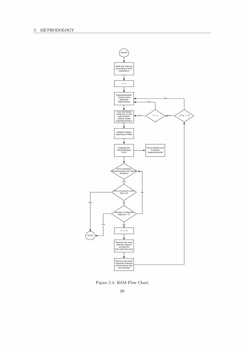
5. METHODOLOGY

START

Rank the features according to their

importance

i = 1

Hyperparameter Tuning using

Bayesian Optimization

Train the Model using the current

pair (feature subset, tuned

hyperparameter)

Update Feature Importance Rank

Evaluate the Generalization

Error

Store Models and Posterior

Hyperparameter

Error increases monotonically over last B

iterations

Error increases more than C%

Number of selected features < D

i = i + 1

Recover the most relevant feature

among the Non-selected ones

Remove two least important features among those that

are selected

STOP

Yes

No

No

Yes

Yes No

i == 1 i % A == 0

Yes

Yes

No No

Figure 5.4: BAM Flow Chart

30

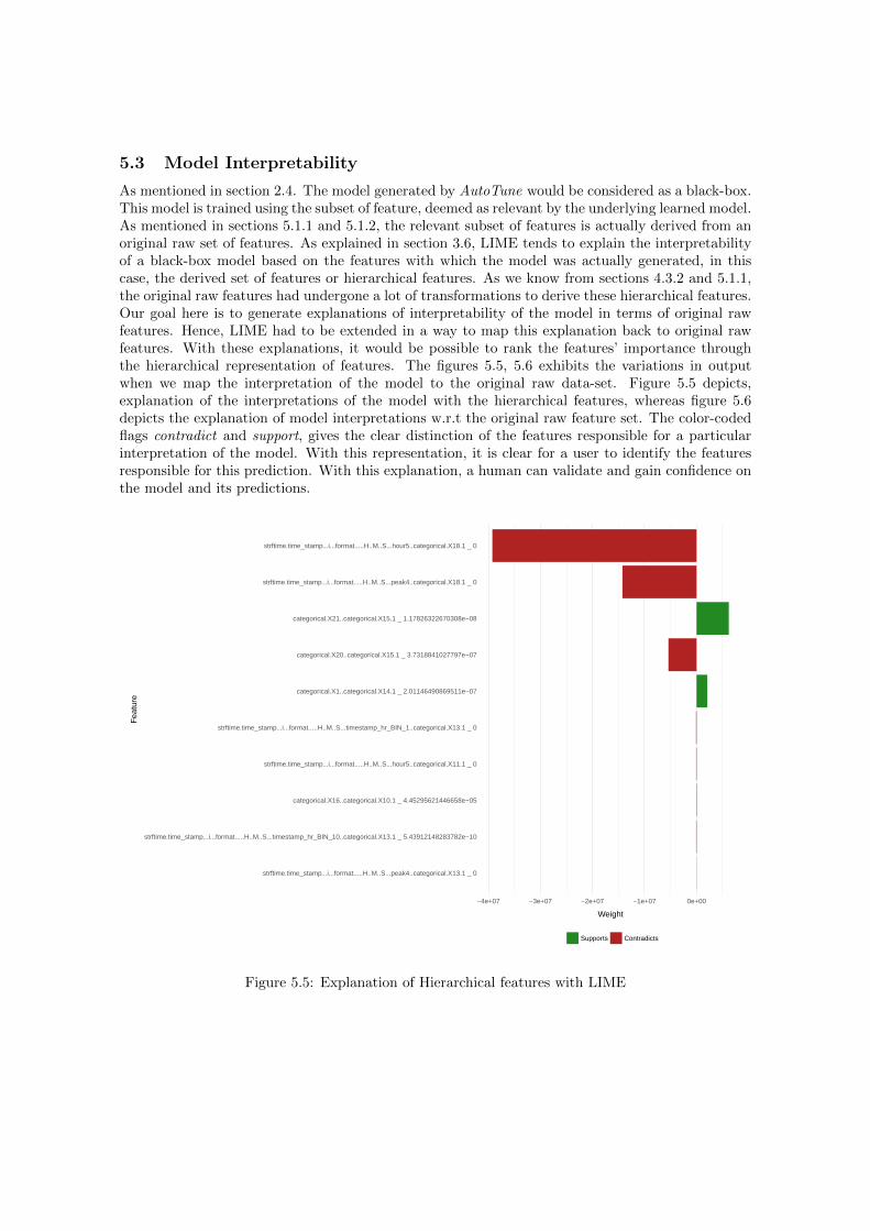
5.3 Model Interpretability

As mentioned in section 2.4. The model generated by AutoTune would be considered as a black-box.This model is trained using the subset of feature, deemed as relevant by the underlying learned model.As mentioned in sections 5.1.1 and 5.1.2, the relevant subset of features is actually derived from anoriginal raw set of features. As explained in section 3.6, LIME tends to explain the interpretabilityof a black-box model based on the features with which the model was actually generated, in thiscase, the derived set of features or hierarchical features. As we know from sections 4.3.2 and 5.1.1,the original raw features had undergone a lot of transformations to derive these hierarchical features.Our goal here is to generate explanations of interpretability of the model in terms of original rawfeatures. Hence, LIME had to be extended in a way to map this explanation back to original rawfeatures. With these explanations, it would be possible to rank the features’ importance throughthe hierarchical representation of features. The figures 5.5, 5.6 exhibits the variations in outputwhen we map the interpretation of the model to the original raw data-set. Figure 5.5 depicts,explanation of the interpretations of the model with the hierarchical features, whereas figure 5.6depicts the explanation of model interpretations w.r.t the original raw feature set. The color-codedflags contradict and support, gives the clear distinction of the features responsible for a particularinterpretation of the model. With this representation, it is clear for a user to identify the featuresresponsible for this prediction. With this explanation, a human can validate and gain confidence onthe model and its predictions.

strftime.time_stamp...i...format.....H..M..S...peak4..categorical.X13.1 _ 0

strftime.time_stamp...i...format.....H..M..S...timestamp_hr_BIN_10..categorical.X13.1 _ 5.43912148283782e−10

categorical.X16..categorical.X10.1 _ 4.45295621446658e−05

strftime.time_stamp...i...format.....H..M..S...hour5..categorical.X11.1 _ 0

strftime.time_stamp...i...format.....H..M..S...timestamp_hr_BIN_1..categorical.X13.1 _ 0






−4e+07 −3e+07 −2e+07 −1e+07 0e+00

Weight

Fea

ture

Supports Contradicts

Figure 5.5: Explanation of Hierarchical features with LIME

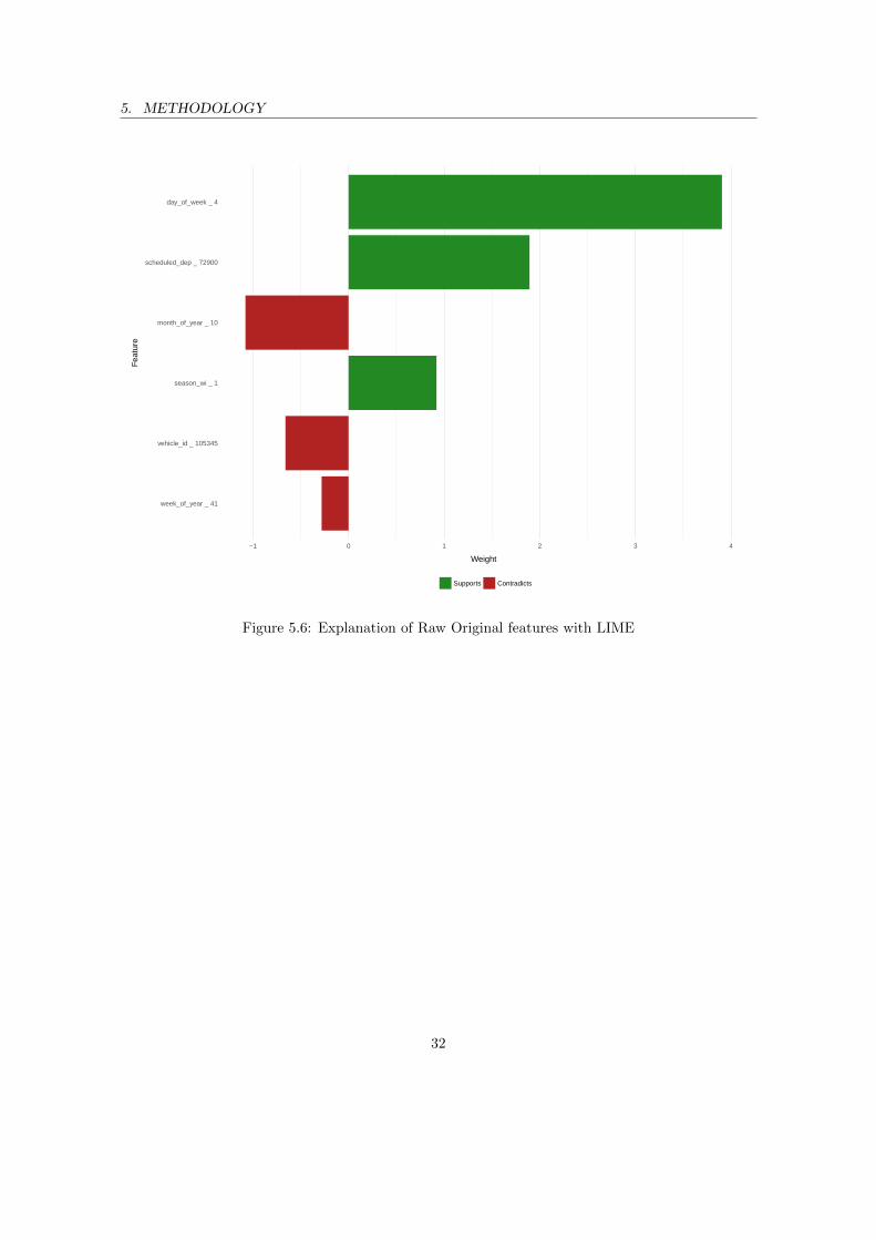
5. METHODOLOGY

week_of_year _ 41

vehicle_id _ 105345

season_wi _ 1

month_of_year _ 10

scheduled_dep _ 72900

day_of_week _ 4

−1 0 1 2 3 4

Weight

Fea

ture


Figure 5.6: Explanation of Raw Original features with LIME

32

6 Experiments

The experiments were conducted using the R Software. Data were divided into two sets: a trainingset and a test set (i.e 70%/30%). As the Ensemble technique62 suggested (i.e. Bucket-of-Models) donot provide better results than the best model in the pool, we end up focusing only on evaluating theperformance of the two proposed feature selection methods (LASSO and AutoTune) using the fiveproposed base learners (RF, SVR, PPR, GBM and NN). The method consists of two types of hy-perparameters: general and model-specific. The setting for the general ones is depicted in Table 6.1.The procedure to obtain the model-specific one is detailed in section 5.2.2.5. We used glmnet [64]procedures for fitting LASSO baseline. The best model was selected using 5-fold cross-validation.The above mentioned five base learners were evaluated based on the two resulting feature spaces: thefeature set given by 1) Baseline LASSO (SoA) and by 2) AutoTune-SRL (Feature selection techniquefrom NLE). The model’s hyperparameter tuning for LASSO is made with Bayesian Optimization.The obtained results were compared using three metrics of interest: NRMSE63 (normalized RMSE,where the normalization constant is the averaged value of the target), RMSE64 and MAE65.

Value Description

φ 1% minimum admissible ratio between the 2nd/1st more frequent values ofa relevant feature

n 95% maximum admissible ratio of invariant values of a relevant featurermax 0.8 maximum admissible Pearson correlation coefficient between two rele-

vant featuresNMIEmin 3.75% minimum Normalized Mean Increasing Error of a relevant featureχ 50% percentage of the best LASSO λ shrinkage coefficient that is used to

define irrelevant featuresω 5 number of iterations in BAM that are required to proceed with a hyper-

parameter tuning stepτ 5 minimum threshold to the number of consecutive iterations in BAM ex-

periencing a monotonic increase in the estimated loss (stopping criteria)κ 30% minimum threshold to the increase of loss estimation in BAM while

compared to the lowest one (stopping criteria)δ 5 minimum threshold to the cardinality of the optimal feature subset in

BAM

Table 6.1: General Hyperparameter Setting

We aim to evaluate few questions mentioned below: a way of comparison between the SoA andthe implementation of AutoTune

• (Q1) Does AutoTune-SRL induced with the five base learners (RF, SVR, PPR, GBM andNN) perform better than SoA?

62Ensemble is a collection or group of certain entities63NRMSE is Normalized Root Mean Square Error64RMSE is Root Mean Square Error is square root of average of squared difference between predicted values by a

model and the values actually observed from the environment that is being modeled65MAE is Mean Absolute Error is the average over the absolute differences between prediction and actual obser-

vation direction

6. EXPERIMENTS

• (Q2) How can we trust the predictions of the base learners? Does LIME integration help usbetter understand the selection of relevant feature subset?

6.1 Experimental Setup

We utilize the caret package [65] from R software to achieve hyperparameter tuning. Package caretprovides us with a range of ML methods (i.e RF, SVR, PPR, GBM and NN). By specifying thetype of method argument, we can use the specific method for consideration during hyperparametertuning. Each base learner mentioned above has its own set of hyperparameters to be tuned.

• RF hyperparameters are the number of randomly selected predictors to choose from at eachsplit mtry and the number of grown trees ntree. The value for the argument method is rf

• SVR hyperparameters are sigma, i.e the distance measure of the support vectors w.r.t tothe hyperplane and C parameter trades-off mis-classification of training samples against thesimplicity of decision surface . The value for the argument method is svmRadial (i.e SVR withRadial Basis Function Kernel)

• PPR hyperparameters are nterms the number of features that should remain the model afteralternate termination of features. maxterms is the upper threshold of the number of featuresallowed. Optlevel is a third hyperparameter which controls how thoroughly the models arerefitted during this process. To smooth the ridge function we need bass and span to fit thecontrol. The value for the argument method is ppr

• GBM hyperparameters are n.trees is the total number of trees to fit. Second parameteris .interaction:depth the maximum depth of variable interactions. The other parameter isn.minobsinnode gives the minimum number of observations in the trees terminal nodes. Fi-nally, shrinkage is a learning rate or step-size reduction measure. The value for the argumentmethod is gbm

• NN hyperparameters are layer1, layer2 and layer3, the complexity of the MLP is controlledby these three parameters. The argument value of each layer denotes the number of nodes tobe considered in that layer. The value for the argument method is mlp

BayesianOptimization function from rBayesianOptimization [66] does the actual hyperparametertuning. BayesianOptimization achieves this by taking in the above-mentioned parameters for eachrespective base learner as arguments and trains a model using caret::train, with a specific methodi.e to tune RF parameters the argument method is set to rf. The model is trained in an iterativeprocess by picking a combination of parameters’ values from a search grid. The trained model isselected from this iterative process and the parameters corresponding to that model is labeled asthe best set of tuned parameters.

By default, we use grid search during training to optimize parameter tuning. The tuning param-eter grid can be specified by the user. The argument tuneGrid can take a data frame with columnsor a range of tuning values for each tuning parameter. The column names should be the same asthe fitting method’s (i.e base learner’s) arguments. Another is to use a random selection of tuningparameter combinations to cover the parameter space to a lesser extent (which is not considered inthis report).

34

6. EXPERIMENTS

In the context of AutoTune-SRL (refer to section 5.2.2), The original feature set is processed togenerate a sparse space of features (refer to section 5.1.1,5.1.2). The generated features are con-sumed by AutoTune-SRL for optimal feature selection (refer to section 5.2.2). After hyperparametertuning with the selected set of features, BAM considers the obtained best parameters as constantfor further optimal selection of feature set (refer to section 5.2.2.5). As mentioned in section 5.1.4,to the models obtained w.r.t each base learner, it’s associated feature set and the tuned base pa-rameters, an ensemble procedure Bucket of models is applied. The model selected would be furtherpost-processed as given in section 5.1.5.

In the context of SoA, the original input features are filtered by LASSO. Generate tuned param-eter set for each base learner w.r.t the obtained feature subset with BayesianOptimization. Then, afinal trained model is obtained by caret::train with the tuned parameters.

The explanation of predictions of the model is achieved by LIME. The LIME package is written inR software is found in reference [67]. The First step is to create an explainer from the main functionof package LIME lime::lime. The explainer is a function that is used to explain the predictions madeby black box model. The continuous variables are binned to get more variation in the explanation,this can be done by setting the argument bin continuous. The explainer function generated fromlime::lime can be used to explain the result of the model on new observations by lime::explainfunction. The explanation obtained is used to explain the relevance of features w.r.t interpretationof each predicted sample.

6.2 Testbeds and Results

In this section, we describe the testbeds built to answer the proposed research questions, pointingout the obtained results.

Q(1). We evaluate the goodness of the AutoTune-SRL feature selection technique with theState-of-the-Art (SoA). This is done by comparison of Generalization Errors (i.e RMSE, NRMSEand MAE). The tables 6.3, 6.4, 6.5, 6.6 and 6.7 exhibits this comparative result. The columnscenario depicts the four stages of post-processing phase (to handle the outliers) and the associatedRMSE, NRMSE and MAE (i.e Generalization Error). The Generalization Error of the Best Modelselected from this post-processing phase (i.e Test Error column) is compared with the GeneralizationError of SoA. The Best Model is highlighted with bold font. The last row features for each routeis the count of adequate features selected after AutoTune-SRL and LASSO. The SoA with all theregression methods has the worst results possible w.r.t to every route A1, A2, B1 and B2. From theregression methods RF, SVR, PPR and GBM show gradual improvement in each post-processingphase as compared to the respective SoA errors. But NN method shows erratic behavior while tryingto implement for two of the post-processing techniques (1) Baseline and (2) Baseline with Tukey.This behavior is consistent with all the above-mentioned routes. More research is required on thispipeline, with NN as the base learner, to identify the root cause of this unwanted behavior. TheAutoTune-SRL outperforms SoA by roughly 32%. The quartile range is given in table 6.2, whichprovides a comparative overview of the results aggregated for all the base learners and SoA. Thebox-plot of the AutoTune-SRL and SoA mentioned comparison is given in figure 6.1.

35

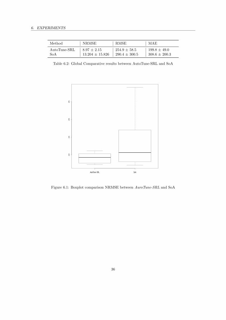
6. EXPERIMENTS

Method NRMSE RMSE MAE

AutoTune-SRL 8.97 ± 2.15 254.9 ± 58.5 199.8 ± 49.0SoA 13.204 ± 15.826 290.4 ± 300.5 308.6 ± 200.3

Table 6.2: Global Comparative results between AutoTune-SRL and SoA

AutoTune−SRL SoA

10

15

20

25

Figure 6.1: Boxplot comparison NRMSE between AuroTune-SRL and SoA

36

6. EXPERIMENTS

Route Scenario SoA

RMSE 236,00

NRMSE 7,57%

MAE 191,91

RMSE 236,93

NRMSE 7,60%

MAE 192,84

RMSE 237,08

NRMSE 7,61%

MAE 193,04

RMSE 236,56

NRMSE 7,59%

MAE 192,53

244 10

RMSE 204,18

NRMSE 7,19%

MAE 162,42

RMSE 203,41

NRMSE 7,17%

MAE 161,30

RMSE 203,77

NRMSE 7,18%

MAE 161,43

RMSE 204,21

NRMSE 7,19%

MAE 162,39

197 9

RMSE 252,74

NRMSE 9,39%

MAE 187,44

RMSE 251,34

NRMSE 9,34%

MAE 184,86

RMSE 250,32

NRMSE 9,30%

MAE 183,94

RMSE 249,41

NRMSE 9,27%

MAE 184,18

343 10

RMSE 268,32

NRMSE 9,67%

MAE 214,78

RMSE 264,40

NRMSE 9,53%

MAE 210,96

RMSE 263,95

NRMSE 9,51%

MAE 210,47

RMSE 268,70

NRMSE 9,68%

MAE 214,72

325 7

Scenario Errors

NRMSE 9,69% 10,63%

MAE 218,17 240,93

186,13 186,64

RMSE 268,86 295,01

RMSE 209,52 203,57

NRMSE 7,38% 7,17%

237,66

NRMSE 7,62% 7,63%

MAE 192,10 189,35

B2

Baseline

Baseline + log

Baseline + log + Tukey

Baseline + Tukey

Baseline

Baseline + log


Baseline + Tukey

B1

features

features

MAE 165,96 161,38

RMSE 251,11 256,83

NRMSE 9,33% 8,54%

MAE

A1

A2

features

features

Baseline

Baseline + log



Baseline + Tukey

Baseline + log

Baseline + Tukey

Baseline

Test Error

RMSE 237,37

Table 6.3: Generalization Error comparison of regression method RF with SoA for all the routes A1, A2 , B1 and B2

37

6. EXPERIMENTS

Route Scenario SoA

RMSE 284,15

NRMSE 9,12%

MAE 221,23

RMSE 286,58

NRMSE 9,20%

MAE 222,91

RMSE 286,56

NRMSE 9,19%

MAE 222,91

RMSE 284,13

NRMSE 9,12%

MAE 221,26

108 10

RMSE 299,56

NRMSE 10,55%

MAE 229,72

RMSE 302,02

NRMSE 10,64%

MAE 231,47

RMSE 302,07

NRMSE 10,64%

MAE 231,51

RMSE 299,72

NRMSE 10,56%

MAE 229,84

99 9

RMSE 391,10

NRMSE 14,53%

MAE 284,62

RMSE 398,48

NRMSE 14,81%

MAE 289,83

RMSE 398,87

NRMSE 14,82%

MAE 290,12

RMSE 392,07

NRMSE 14,57%

MAE 285,27

136 10

RMSE 329,10

NRMSE 11,86%

MAE 256,66

RMSE 328,36

NRMSE 11,84%

MAE 256,33

RMSE 328,36

NRMSE 11,84%

MAE 256,34

RMSE 328,94

NRMSE 11,86%

MAE 256,57

92 7

Scenario Errors

A1

A2

features

features

Baseline

Baseline + log



Baseline + Tukey

Baseline

Baseline + log

Baseline + Tukey

features

features

B2

B1

Baseline + Tukey

Baseline

Baseline + log


Baseline + Tukey


Baseline

Baseline + log

Test Error

RMSE 237,30 506,90

NRMSE 7,61% 16,26%

MAE 189,46 418,07

RMSE 222,44 532,97

NRMSE 7,84% 18,78%

MAE 175,84 435,85

RMSE 277,23 561,71

NRMSE 10,30% 20,87%

MAE 207,12 450,52

RMSE 294,72 495,21

NRMSE 10,62% 17,85%

MAE 231,44 393,56

Table 6.4: Generalization Error comparison of regression method SVR with SoA for all the routesA1 , A2 , B1 and B2

38

6. EXPERIMENTS

Route Scenario SoA

RMSE 243,12

NRMSE 7,80%

MAE 196,75

RMSE 244,08

NRMSE 7,83%

MAE 198,35

RMSE 243,52

NRMSE 7,81%

MAE 198,10

RMSE 241,34

NRMSE 7,74%

MAE 195,85

170 10

RMSE 205,93

NRMSE 7,26%

MAE 161,57

RMSE 207,21

NRMSE 7,30%

MAE 162,00

RMSE 206,79

NRMSE 7,29%

MAE 161,78

RMSE 206,89

NRMSE 7,29%

MAE 162,17

174 9

RMSE 256,77

NRMSE 9,55%

MAE 196,57

RMSE 262,36

NRMSE 9,75%

MAE 199,88

RMSE 261,18

NRMSE 9,71%

MAE 199,51

RMSE 261,09

NRMSE 9,70%

MAE 201,46

232 10

RMSE 289,45

NRMSE 10,43%

MAE 230,79

RMSE 274,06

NRMSE 9,88%

MAE 218,02

RMSE 270,05

NRMSE 9,73%

MAE 214,50

RMSE 275,53

NRMSE 9,93%

MAE 219,32

176 7

RMSE 291,30 243,39

NRMSE 10,36% 10,62%

MAE 206,24 206,13

features


Baseline + Tukey

B1

B2

features


Baseline + Tukey

Baseline

Baseline + log

Baseline

Baseline + log

194,65

RMSE 204,57 235,20

NRMSE 7,21% 8,29%

241,06

NRMSE 7,62% 7,75%

A2

features


Baseline + Tukey


Baseline + Tukey

Baseline

Baseline + log

Baseline

Baseline + log

features

MAE

A1

Scenario Errors Test Error

RMSE 237,37

192,10

MAE 161,65 187,85

RMSE 278,85 285,75

NRMSE 10,50% 8,77%

MAE 227,60 192,08

Table 6.5: Generalization Error comparison of regression method PPR with SoA for all the routesA1 , A2 , B1 and B2

39

6. EXPERIMENTS

Route Scenario SoA

RMSE 376,51

NRMSE 12,08%

MAE 304,79

RMSE 239,86

NRMSE 7,69%

MAE 194,11

RMSE 292,06

NRMSE 9,37%

MAE 239,42

RMSE 1095,40

NRMSE 35,15%

MAE 1034,88

262 10

RMSE 777,63

NRMSE 27,39%

MAE 705,85

RMSE 229,10

NRMSE 8,07%

MAE 171,23

RMSE 234,78

NRMSE 8,27%

MAE 194,42

RMSE 1045,68

NRMSE 30,67%

MAE 1048,67

245 9

RMSE 634,16

NRMSE 23,57%

MAE 525,64

RMSE 250,23

NRMSE 9,30%

MAE 184,17

RMSE 260,80

NRMSE 9,69%

MAE 186,75

RMSE 2339,52

NRMSE 86,94%

MAE 2304,87

354 10

RMSE 513,98

NRMSE 18,53%

MAE 435,32

RMSE 282,84

NRMSE 10,19%

MAE 219,96

RMSE 279,47

NRMSE 10,07%

MAE 216,98

RMSE 347,93

NRMSE 12,54%

MAE 269,85

317 7

Scenario Errors Test Error

A1

BaselineRMSE 271,72

features

features

904,76

Baseline + log

NRMSE 8,72% 29,03%


MAE 222,39 239,28Baseline + Tukey

249,53 421,44

A2

BaselineRMSE 308,80 388,52

Baseline + log

NRMSE 10,88% 13,69%



9,27% 15,66%



B2

BaselineRMSE

B1

Baseline


MAE

Baseline + log

NRMSE

Baseline + log

NRMSE

RMSE

248,85 662,41Baseline + Tukey

features

features

308,50 741,06

11,12% 26,71%

Table 6.6: Generalization Error comparison of regression method NN with SoA for all the routes A1, A2 , B1 and B2

40

6. EXPERIMENTS

Route Scenario SoA

RMSE 234,78

NRMSE 7,53%

MAE 190,78

RMSE 233,67

NRMSE 7,50%

MAE 189,87

RMSE 233,55

NRMSE 7,49%

MAE 189,60

RMSE 232,91

NRMSE 7,47%

MAE 188,66

266 10

RMSE 206,06

NRMSE 7,26%

MAE 163,00

RMSE 204,94

NRMSE 7,22%

MAE 162,00

RMSE 205,17

NRMSE 7,23%

MAE 162,33

RMSE 206,09

NRMSE 7,26%

MAE 163,32

252 9

RMSE 249,53

NRMSE 9,27%

MAE 185,14

RMSE 250,11

NRMSE 9,29%

MAE 184,69

RMSE 248,84

NRMSE 9,25%

MAE 182,92

RMSE 249,41

NRMSE 9,27%

MAE 184,18

265 10

RMSE 264,09

NRMSE 9,51%

MAE 211,97

RMSE 256,80

NRMSE 9,26%

MAE 206,05

RMSE 254,95

NRMSE 9,19%

MAE 204,57

RMSE 259,08

NRMSE 9,34%

MAE 208,18

325 7

B2

Baseline262,20 323,41

Baseline + Tukey

features

9,45% 11,66%

210,65 271,14

RMSE

NRMSE

MAE

Baseline + log


258,99

Baseline + Tukey

features

RMSE

NRMSE

MAE

9,23% 9,62%

183,49 187,79

Baseline + log


A2

Baseline204,93

B1

Baseline248,42

201,14

Baseline + Tukey

features

Baseline + log


RMSE

NRMSE

MAE

181,75

7,21% 7,09%

162,09 161,37

Baseline + log


Scenario Errors

A1

Baseline233,75 232,12

Baseline + Tukey

features

RMSE

NRMSE

Test Error

MAE

7,50% 7,45%

189,66

Table 6.7: Generalization Error comparison Table of regression method GBM with SoA for all theroutes A1 , A2 , B1 and B2

41

6. EXPERIMENTS

Q(2). The LIME explanations are obtained for black-box models from RF, SVR, PPR andGBM. The NN black box model is exempted from this experiment because of its erratic behavioras observed in the experiment of the research question (Q1). We have taken 2 sets of features(1) The Original Feature set (i.e day of week, month of year, scheduled dep, season wi, veh id,week of year) and (2) Clusterized feature set (i.e day of week, month of year, scheduled dep, sea-son wi, veh id cluster1, veh id cluster2, veh id cluster3, veh id cluster4, week of year). The secondset of features are obtained by clustering the categorical feature veh id with Gaussian Mixture Modeltrained using the Expectation-Maximization algorithm. We seek to achieve explanations for these 2sets of features for each black-box model from the base learners mentioned above. Each set of thefeature is represented by two charts bar and line, distributed over the week.

The explanations for each model is obtained for each route A1, A2, B1 and B2. We will berelying on some of the charts which exhibits extreme diversity w.r.t to each route. A global view ofthe graphs is given below. One can conclude that the busy days are during the Weekdays (Monday,Tuesday, Wednesday, Thursday and Friday). The busiest among that is on Monday. On the Week-ends the days or not so busy for the TMS. The best results for route A1 with varying differences infeatures’ adequacy is represented by figures 6.2 and 6.3, the underlying learner is RF. Similarly, forroute A2, the best feature representation is portrayed by the underlying learner SVR with figures6.4 and 6.5. For route B1, the best variations among features are shown in figures 6.6 and 6.7,generated by the learner GBM. For the route B2, the learner PPR generates the best results, whichis shown in figures 6.8 and 6.9.

Now, with the overview of the explanations obtained from each route. Let us check the ef-fectiveness of the extended LIME for each learner with a single randomly selected sample from asingle dataset A1. Here again, we consider 2 sets of features (1) The Original feature set and (2)the Clusterized feature set. As the clusterized set of features are derived from the original ones, itwould be better to see the variations in the results at each level of the hierarchical structure. Thevalues associated with the randomly selected sample data are: vehicle id : 105373, week of year: 46, day of week : 5, scheduled dep : 60300, season wi : 1, month of year : 11. Now with thissetup, we are able to compare the adequate selection of our AutoML pipeline. The color-coded flags(i.e support and contradict) gives an accurate representation of which features are considered asadequate by each respective learners. The adequacy of features for learner PPR is represented byfigures 6.10 and 6.11. SVR representation of adequate features is depicted by figures 6.12 and 6.13.RF is represented by figures 6.14 and 6.15. Finally, figures 6.16 and 6.17 represent the adequatefeatures of GBM.

42

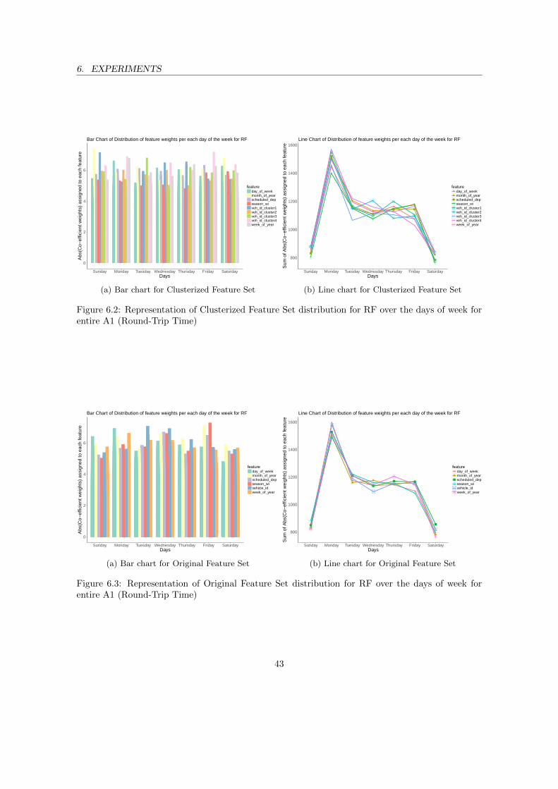
6. EXPERIMENTS

0

2

4

6

Sunday Monday Tuesday Wednesday Thursday Friday SaturdayDays

Abs

(Co−

effic

ient

wei

ghts

) as

sign

ed to

eac

h fe

atur

e

featureday_of_weekmonth_of_yearscheduled_depseason_wiveh_id_cluster1veh_id_cluster2veh_id_cluster3veh_id_cluster4week_of_year

Bar Chart of Distribution of feature weights per each day of the week for RF

(a) Bar chart for Clusterized Feature Set

●

●

●

●

●

●

●800

1000

1200

1400

1600


Sum

of A

bs(C

o−ef

ficie

nt w

eigh

ts)

assi

gned

to e

ach

feat

ure

feature● day_of_week

month_of_yearscheduled_depseason_wiveh_id_cluster1veh_id_cluster2veh_id_cluster3veh_id_cluster4week_of_year

Line Chart of Distribution of feature weights per each day of the week for RF

(b) Line chart for Clusterized Feature Set

Figure 6.2: Representation of Clusterized Feature Set distribution for RF over the days of week forentire A1 (Round-Trip Time)

0

2

4

6


Abs

(Co−

effic

ient

wei

ghts

) as

sign

ed to

eac

h fe

atur

e

featureday_of_weekmonth_of_yearscheduled_depseason_wivehicle_idweek_of_year

Bar Chart of Distribution of feature weights per each day of the week for RF

(a) Bar chart for Original Feature Set

●

●

●

● ●

●

●

800

1000

1200

1400

1600


Sum

of A

bs(C

o−ef

ficie

nt w

eigh

ts)

assi

gned

to e

ach

feat

ure


month_of_yearscheduled_depseason_wivehicle_idweek_of_year

Line Chart of Distribution of feature weights per each day of the week for RF

(b) Line chart for Original Feature Set

Figure 6.3: Representation of Original Feature Set distribution for RF over the days of week forentire A1 (Round-Trip Time)

43

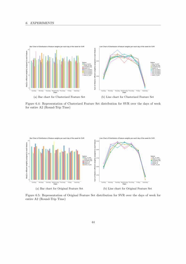
6. EXPERIMENTS

0

5

10

15


Abs

(Co−

effic

ient

wei

ghts

) as

sign

ed to

eac

h fe

atur

e


Bar Chart of Distribution of feature weights per each day of the week for SVR


●

●

●

●

●

●

●

1500

2000


Sum

of A

bs(C

o−ef

ficie

nt w

eigh

ts)

assi

gned

to e

ach

feat

ure



Line Chart of Distribution of feature weights per each day of the week for SVR


Figure 6.4: Representation of Clusterized Feature Set distribution for SVR over the days of weekfor entire A2 (Round-Trip Time)

0

5

10

15


Abs

(Co−

effic

ient

wei

ghts

) as

sign

ed to

eac

h fe

atur

e


Bar Chart of Distribution of feature weights per each day of the week for SVR


●

●

●

●

●

●

●1250

1500

1750

2000

2250


Sum

of A

bs(C

o−ef

ficie

nt w

eigh

ts)

assi

gned

to e

ach

feat

ure



Line Chart of Distribution of feature weights per each day of the week for SVR


Figure 6.5: Representation of Original Feature Set distribution for SVR over the days of week forentire A2 (Round-Trip Time)

44

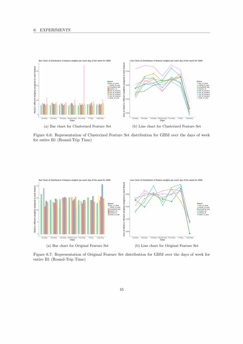
6. EXPERIMENTS

0

20

40

60


Abs

(Co−

effic

ient

wei

ghts

) as

sign

ed to

eac

h fe

atur

e


Bar Chart of Distribution of feature weights per each day of the week for GBM


●

●

●

●

●

●

●

2000

2250

2500

2750


Sum

of A

bs(C

o−ef

ficie

nt w

eigh

ts)

assi

gned

to e

ach

feat

ure



Line Chart of Distribution of feature weights per each day of the week for GBM


Figure 6.6: Representation of Clusterized Feature Set distribution for GBM over the days of weekfor entire B1 (Round-Trip Time)

0

5

10

15

20


Abs

(Co−

effic

ient

wei

ghts

) as

sign

ed to

eac

h fe

atur

e


Bar Chart of Distribution of feature weights per each day of the week for GBM


●

●

●

●

●

●

●

2000

2200

2400

2600


Sum

of A

bs(C

o−ef

ficie

nt w

eigh

ts)

assi

gned

to e

ach

feat

ure



Line Chart of Distribution of feature weights per each day of the week for GBM


Figure 6.7: Representation of Original Feature Set distribution for GBM over the days of week forentire B1 (Round-Trip Time)

45

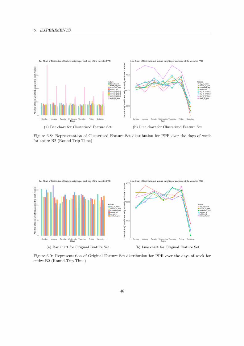
6. EXPERIMENTS

0

30

60

90


Abs

(Co−

effic

ient

wei

ghts

) as

sign

ed to

eac

h fe

atur

e


Bar Chart of Distribution of feature weights per each day of the week for PPR


●

●

●

●

●

●

●

3500

4000

4500


Sum

of A

bs(C

o−ef

ficie

nt w

eigh

ts)

assi

gned

to e

ach

feat

ure



Line Chart of Distribution of feature weights per each day of the week for PPR


Figure 6.8: Representation of Clusterized Feature Set distribution for PPR over the days of weekfor entire B2 (Round-Trip Time)

0

10

20

30


Abs

(Co−

effic

ient

wei

ghts

) as

sign

ed to

eac

h fe

atur

e


Bar Chart of Distribution of feature weights per each day of the week for PPR


●

●

●

● ●

●

●

3500

4000

4500


Sum

of A

bs(C

o−ef

ficie

nt w

eigh

ts)

assi

gned

to e

ach

feat

ure



Line Chart of Distribution of feature weights per each day of the week for PPR


Figure 6.9: Representation of Original Feature Set distribution for PPR over the days of week forentire B2 (Round-Trip Time)

46

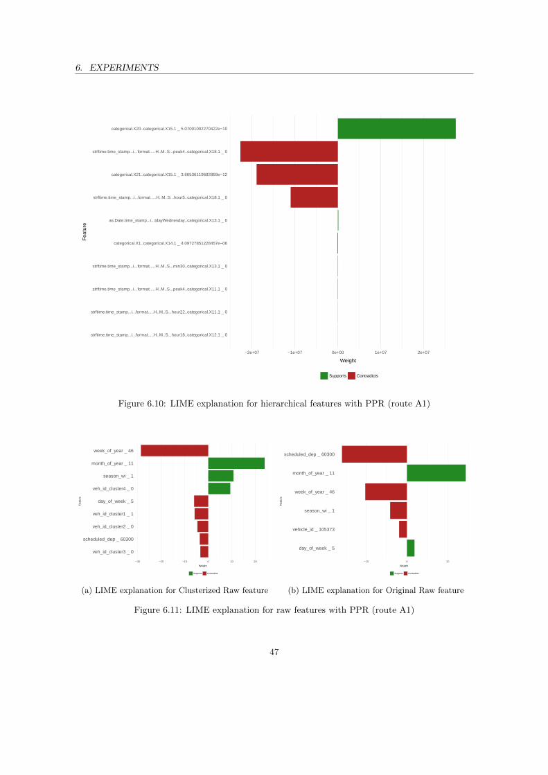
6. EXPERIMENTS




strftime.time_stamp...i...format.....H..M..S...min30..categorical.X13.1 _ 0


as.Date.time_stamp...i...tdayWednesday..categorical.X13.1 _ 0





−2e+07 −1e+07 0e+00 1e+07 2e+07

Weight

Fea

ture


Figure 6.10: LIME explanation for hierarchical features with PPR (route A1)

veh_id_cluster3 _ 0


veh_id_cluster2 _ 0

veh_id_cluster1 _ 1

day_of_week _ 5

veh_id_cluster4 _ 0

season_wi _ 1

month_of_year _ 11

week_of_year _ 46

−30 −20 −10 0 10 20

Weight

Fea

ture


(a) LIME explanation for Clusterized Raw feature

day_of_week _ 5

vehicle_id _ 105373

season_wi _ 1

week_of_year _ 46

month_of_year _ 11


−10 0 10

Weight

Fea

ture


(b) LIME explanation for Original Raw feature

Figure 6.11: LIME explanation for raw features with PPR (route A1)

47

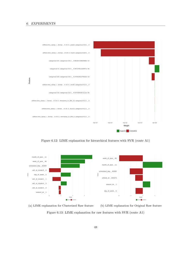
6. EXPERIMENTS











−8e+07 −6e+07 −4e+07 −2e+07 0e+00

Weight

Fea

ture


Figure 6.12: LIME explanation for hierarchical features with SVR (route A1)

season_wi _ 1

veh_id_cluster2 _ 0

veh_id_cluster4 _ 0

veh_id_cluster1 _ 1

day_of_week _ 5

veh_id_cluster3 _ 0


week_of_year _ 46

month_of_year _ 11

−3 0 3 6

Weight

Fea

ture



day_of_week _ 5

season_wi _ 1

vehicle_id _ 105373


month_of_year _ 11

week_of_year _ 46

−8 −4 0 4

Weight

Fea

ture



Figure 6.13: LIME explanation for raw features with SVR (route A1)

48

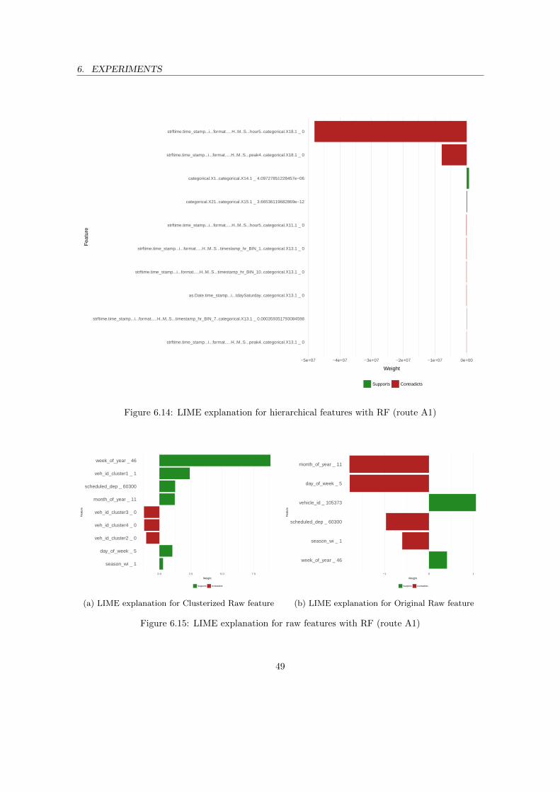
6. EXPERIMENTS


strftime.time_stamp...i...format.....H..M..S...timestamp_hr_BIN_7..categorical.X13.1 _ 0.000359351793084598

as.Date.time_stamp...i...tdaySaturday..categorical.X13.1 _ 0








−5e+07 −4e+07 −3e+07 −2e+07 −1e+07 0e+00

Weight

Fea

ture


Figure 6.14: LIME explanation for hierarchical features with RF (route A1)

season_wi _ 1

day_of_week _ 5

veh_id_cluster2 _ 0

veh_id_cluster4 _ 0

veh_id_cluster3 _ 0

month_of_year _ 11


veh_id_cluster1 _ 1

week_of_year _ 46

0.0 2.5 5.0 7.5

Weight

Fea

ture



week_of_year _ 46

season_wi _ 1


vehicle_id _ 105373

day_of_week _ 5

month_of_year _ 11

−1 0 1

Weight

Fea

ture



Figure 6.15: LIME explanation for raw features with RF (route A1)

49

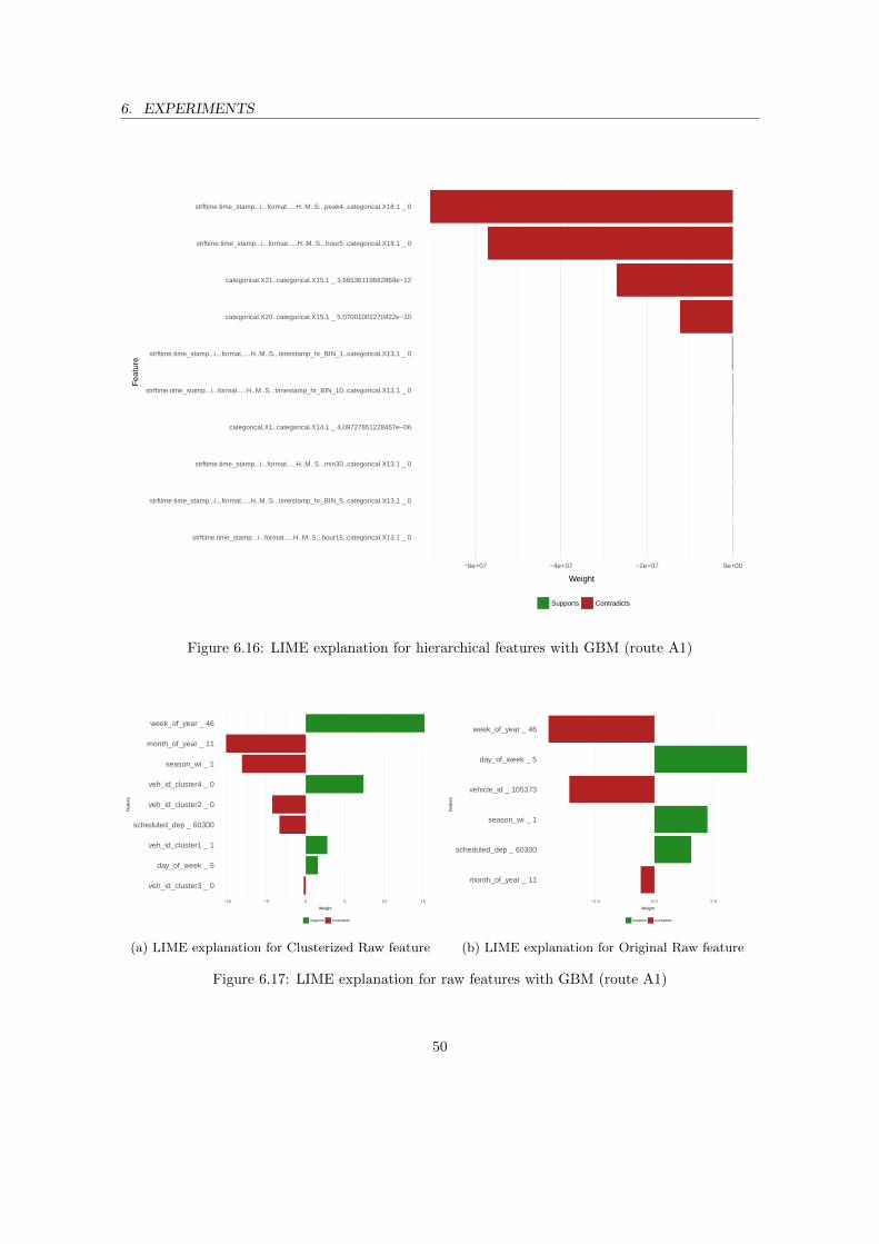
6. EXPERIMENTS











−6e+07 −4e+07 −2e+07 0e+00

Weight

Fea

ture


Figure 6.16: LIME explanation for hierarchical features with GBM (route A1)

veh_id_cluster3 _ 0

day_of_week _ 5

veh_id_cluster1 _ 1


veh_id_cluster2 _ 0

veh_id_cluster4 _ 0

season_wi _ 1

month_of_year _ 11

week_of_year _ 46

−10 −5 0 5 10 15

Weight

Fea

ture



month_of_year _ 11


season_wi _ 1

vehicle_id _ 105373

day_of_week _ 5

week_of_year _ 46

−2.5 0.0 2.5

Weight

Fea

ture



Figure 6.17: LIME explanation for raw features with GBM (route A1)

50

7 Concluding Remarks

In conclusion, this thesis focused on two important aspects of an AutoML pipeline. First, auto-mated selection of adequate feature subset from the hierarchical feature space. This was achievedby implementing an NLE developed AutoML pipeline called AutoTune. AutoTune followed shallowrepresentation learning technique, which used the combination of well known filter methods andan NLE developed procedure BAM. The performance of this NLE implemented feature selectionapproach is measured against a well known SoA. From the results of Q1 (refer to section 6.2) , wecan observe that there was a 32% improvement in the newly implemented approach as compared tothe SoA.

The second aspect of the AutoML was to implement a way to explain model interpretations. Theend result of the AutoTune pipeline is a model trained with the hierarchical features space. We usedLIME tool approach to explaining these interpretations. There was a drawback with this approach,i.e explaining the interpretations of the model w.r.t to these hierarchical features would not be agood representation for the users to bank on. However, we extended LIME to map the explanationsof the model to the original raw feature set. The results obtained were easily understandable by hu-mans and the interpretations of the model clearly describe the adequacy of the features responsiblefor the predictions.

7.1 Future Work

Despite the insights achieved by the present approach, it also exhibited a minor drawback. Dif-ferent base learners showed to perform better in different contexts. However, NN base learner didnot provide the expected result. As NN is a powerful ML algorithm, more research is required tounderstand the unwanted behavior. Also, resolving this issue could be the key to setup AutoMLpipeline with the unsupervised approach.

Feature selection has been the sole focus of this thesis work. A literature by Brown et. al [68],suggests that stability is a key factor based on which the different Feature selection techniques canbe evaluated. Integrating this concept with our current pipeline approach would give a clear-cutunderstanding if the implemented feature selection algorithm is better suited with this pipeline. Also,stability check can be a varying factor during the model selection process, which is now completelyrelied on the comparison of generalization error.

Bibliography

[1] “Nec laboratories europe gmbh.” https://uk.nec.com/en_GB/emea/about/neclab_eu. Ac-cessed: 2018-04-03.

[2] “A gentle introduction to random forests, ensembles, and performance metrics ina commercial system.” http://blog.citizennet.com/blog/2012/11/10/random-forests-

ensembles-and-performance-metrics. Accessed: 2018-03-31.

[3] “Support vector machine (svm) tutorial.” https://blog.statsbot.co/support-vector-

machines-tutorial-c1618e635e93. Accessed: 2018-03-31.

[4] “Gradient boosting from scratch.” https://medium.com/mlreview/gradient-boosting-

from-scratch-1e317ae4587d. Accessed: 2018-04-07.

[5] “A quick introduction to neural networks.” https://ujjwalkarn.me/2016/08/09/quick-

intro-neural-networks. Accessed: 2018-03-31.

[6] “Introduction to local interpretable model-agnostic explanations (lime).” https:

//www.kdnuggets.com/2016/08/introduction-local-interpretable-model-agnostic-

explanations-lime.html. Accessed: 2018-03-30.

[7] M. T. Ribeiro, S. Singh, and C. Guestrin, “Why should i trust you?: Explaining the predic-tions of any classifier,” in Proceedings of the 22nd ACM SIGKDD International Conference onKnowledge Discovery and Data Mining, pp. 1135–1144, ACM, 2016.

[8] I. H. Witten, E. Frank, M. A. Hall, and C. J. Pal, Data Mining: Practical machine learningtools and techniques. Morgan Kaufmann, 2016.

[9] “Machine learning for automated algorithm design.” http://www.ml4aad.org/automl/. Ac-cessed: 2018-03-30.

[10] L. Kotthoff, C. Thornton, H. H. Hoos, F. Hutter, and K. Leyton-Brown, “Auto-weka 2.0:Automatic model selection and hyperparameter optimization in weka,” The Journal of MachineLearning Research, vol. 18, no. 1, pp. 826–830, 2017.

[11] I. Guyon and A. Elisseeff, “An introduction to variable and feature selection,” Journal ofmachine learning research, vol. 3, no. Mar, pp. 1157–1182, 2003.

[12] “An introduction to feature selection.” https://machinelearningmastery.com/an-

introduction-to-feature-selection/. Accessed: 2018-03-30.

[13] A. Grover and J. Leskovec, “node2vec: Scalable feature learning for networks,” in Proceedingsof the 22nd ACM SIGKDD international conference on Knowledge discovery and data mining,pp. 855–864, ACM, 2016.

[14] N. Srivastava, G. Hinton, A. Krizhevsky, I. Sutskever, and R. Salakhutdinov, “Dropout: Asimple way to prevent neural networks from overfitting,” The Journal of Machine LearningResearch, vol. 15, no. 1, pp. 1929–1958, 2014.

[15] M. Feurer, A. Klein, K. Eggensperger, J. Springenberg, M. Blum, and F. Hutter, “Efficient androbust automated machine learning,” in Advances in Neural Information Processing Systems,pp. 2962–2970, 2015.

52

https://uk.nec.com/en_GB/emea/about/neclab_eu

http://blog.citizennet.com/blog/2012/11/10/random-forests-ensembles-and-performance-metrics

http://blog.citizennet.com/blog/2012/11/10/random-forests-ensembles-and-performance-metrics

https://blog.statsbot.co/support-vector-machines-tutorial-c1618e635e93

https://blog.statsbot.co/support-vector-machines-tutorial-c1618e635e93

https://medium.com/mlreview/gradient-boosting-from-scratch-1e317ae4587d

https://medium.com/mlreview/gradient-boosting-from-scratch-1e317ae4587d

https://ujjwalkarn.me/2016/08/09/quick-intro-neural-networks

https://ujjwalkarn.me/2016/08/09/quick-intro-neural-networks

https://www.kdnuggets.com/2016/08/introduction-local-interpretable-model-agnostic-explanations-lime.html



http://www.ml4aad.org/automl/

https://machinelearningmastery.com/an-introduction-to-feature-selection/

https://machinelearningmastery.com/an-introduction-to-feature-selection/

[16] L. Li, K. Jamieson, G. DeSalvo, A. Rostamizadeh, and A. Talwalkar, “Hyperband: A novelbandit-based approach to hyperparameter optimization,” arXiv preprint arXiv:1603.06560,2016.

[17] J. Snoek, H. Larochelle, and R. P. Adams, “Practical bayesian optimization of machine learningalgorithms,” in Advances in neural information processing systems, pp. 2951–2959, 2012.

[18] C. Thornton, F. Hutter, H. H. Hoos, and K. Leyton-Brown, “Auto-weka: Combined selectionand hyperparameter optimization of classification algorithms,” in Proceedings of the 19th ACMSIGKDD international conference on Knowledge discovery and data mining, pp. 847–855, ACM,2013.

[19] H. Mendoza, A. Klein, M. Feurer, J. T. Springenberg, and F. Hutter, “Towards automatically-tuned neural networks,” in Workshop on Automatic Machine Learning, pp. 58–65, 2016.

[20] K. Eggensperger, M. Feurer, F. Hutter, J. Bergstra, J. Snoek, H. Hoos, and K. Leyton-Brown,“Towards an empirical foundation for assessing bayesian optimization of hyperparameters,” inNIPS workshop on Bayesian Optimization in Theory and Practice, vol. 10, 2013.

[21] M. T. Ribeiro, S. Singh, and C. Guestrin, “Model-agnostic interpretability of machine learning,”arXiv preprint arXiv:1606.05386, 2016.

[22] M. T. Ribeiro, S. Singh, and C. Guestrin, “Anchors: High-precision model-agnostic explana-tions,” AAAI, 2018.

[23] “Decision trees in machine learning.” https://towardsdatascience.com/decision-trees-

in-machine-learning-641b9c4e8052. Accessed: 2018-03-31.

[24] L. Breiman, “Random forests,” Machine learning, vol. 45, no. 1, pp. 5–32, 2001.

[25] C. Cortes and V. Vapnik, “Support-vector networks,” Machine learning, vol. 20, no. 3, pp. 273–297, 1995.

[26] J. H. Friedman and W. Stuetzle, “Projection pursuit regression,” Journal of the Americanstatistical Association, vol. 76, no. 376, pp. 817–823, 1981.

[27] A. Pinkus, Ridge Functions. Cambridge Tracts in Mathematics, Cambridge University Press,2015.

[28] J. Luedicke, “Friedman’s super smoother,”

[29] “A gentle introduction to the gradient boosting algorithm for machine learning.”https://machinelearningmastery.com/gentle-introduction-gradient-boosting-

algorithm-machine-learning/. Accessed: 2018-03-31.

[30] J. Akosa, “Predictive accuracy: A misleading performance measure for highly imbalanced data,”in Proceedings of the SAS Global Forum, 2017.

[31] L. Moreira-Matias, J. Mendes-Moreira, J. F. de Sousa, and J. Gama, “Improving mass transitoperations by using avl-based systems: A survey,” IEEE Transactions on Intelligent Trans-portation Systems, vol. 16, no. 4, pp. 1636–1653, 2015.

53

https://towardsdatascience.com/decision-trees-in-machine-learning-641b9c4e8052

https://towardsdatascience.com/decision-trees-in-machine-learning-641b9c4e8052

https://machinelearningmastery.com/gentle-introduction-gradient-boosting-algorithm-machine-learning/

https://machinelearningmastery.com/gentle-introduction-gradient-boosting-algorithm-machine-learning/

[32] “Japan’s infamous dedication to punctuality meant they apologized for a train being 20 sec-onds early.” https://qz.com/1132306/japans-infamous-dedication-punctuality-meant-

they-apologized-for-a-train-being-20-seconds-early/. Accessed: 2018-03-30.

[33] “Overview of the main passengers’ rights regulations.” https://www.bahn.com/en/view/

booking-information/passenger-rights/passenger-rights-in-rail-transport.shtml.Accessed: 2018-03-30.

[34] U. Carrascal, “A review of travel time estimation and forecasting for advanced traveler infor-mation systems,” Master’s thesis. Universidad del Pais Vasco, 2012.

[35] J. Mendes-Moreira, A. M. Jorge, J. F. de Sousa, and C. Soares, “Comparing state-of-the-artregression methods for long term travel time prediction,” Intelligent Data Analysis, vol. 16,no. 3, pp. 427–449, 2012.

[36] S. I.-J. Chien, Y. Ding, and C. Wei, “Dynamic bus arrival time prediction with artificial neuralnetworks,” Journal of Transportation Engineering, vol. 128, no. 5, pp. 429–438, 2002.

[37] R. Rajbhandari, “Bus arrival time prediction using stochastic time series and markov chains.,”2004.

[38] J. Dong, L. Zou, and Y. Zhang, “Mixed model for prediction of bus arrival times,” in Evolu-tionary Computation (CEC), 2013 IEEE Congress on, pp. 2918–2923, IEEE, 2013.

[39] O. Cats and G. Loutos, “Real-time bus arrival information system: an empirical evaluation,”Journal of Intelligent Transportation Systems, vol. 20, no. 2, pp. 138–151, 2016.

[40] F. Cathey and D. Dailey, “A prescription for transit arrival/departure prediction using auto-matic vehicle location data,” Transportation Research Part C: Emerging Technologies, vol. 11,no. 3-4, pp. 241–264, 2003.

[41] Z.-R. Peng, “A methodology for design of a gis-based automatic transit traveler informationsystem,” Computers, environment and urban systems, vol. 21, no. 5, pp. 359–372, 1997.

[42] Z. Wall and D. Dailey, “An algorithm for predicting the arrival time of mass transit vehicles us-ing automatic vehicle location data,” in in 78th Annual Meeting of the Transportation ResearchBoard, National Research Council, Washington DC, Citeseer, 1999.

[43] L. Moreira-Matias, J. Gama, J. Mendes-Moreira, and J. F. de Sousa, “An incremental proba-bilistic model to predict bus bunching in real-time,” in International Symposium on IntelligentData Analysis, pp. 227–238, Springer, 2014.

[44] L. Moreira-Matias, O. Cats, J. Gama, J. Mendes-Moreira, and J. F. de Sousa, “An onlinelearning approach to eliminate bus bunching in real-time,” Applied Soft Computing, vol. 47,pp. 460–482, 2016.

[45] R. G. Mishalani, M. R. McCord, and S. Forman, “Schedule-based and autoregressive bus run-ning time modeling in the presence of driver-bus heterogeneity,” in Computer-Aided Systems inPublic Transport, pp. 301–317, Springer, 2008.

[46] M. Berkow, A. El-Geneidy, R. Bertini, and D. Crout, “Beyond generating transit performancemeasures: visualizations and statistical analysis with historical data,” Transportation ResearchRecord: Journal of the Transportation Research Board, no. 2111, pp. 158–168, 2009.

54

https://qz.com/1132306/japans-infamous-dedication-punctuality-meant-they-apologized-for-a-train-being-20-seconds-early/

https://qz.com/1132306/japans-infamous-dedication-punctuality-meant-they-apologized-for-a-train-being-20-seconds-early/

https://www.bahn.com/en/view/booking-information/passenger-rights/passenger-rights-in-rail-transport.shtml

https://www.bahn.com/en/view/booking-information/passenger-rights/passenger-rights-in-rail-transport.shtml

[47] A. M. El-Geneidy, J. Horning, and K. J. Krizek, “Analyzing transit service reliability usingdetailed data from automatic vehicular locator systems,” Journal of Advanced Transportation,vol. 45, no. 1, pp. 66–79, 2011.

[48] E. Mazloumi, G. Rose, G. Currie, and M. Sarvi, “An integrated framework to predict bus traveltime and its variability using traffic flow data,” Journal of Intelligent Transportation Systems,vol. 15, no. 2, pp. 75–90, 2011.

[49] M. Robnik-Sikonja and I. Kononenko, “An adaptation of relief for attribute estimation in regres-sion,” in Machine Learning: Proceedings of the Fourteenth International Conference (ICML’97),pp. 296–304, 1997.

[50] S. M. Hassan, L. Moreira-Matias, J. Khiari, and O. Cats, “Feature selection issues in long-termtravel time prediction,” in International Symposium on Intelligent Data Analysis, pp. 98–109,Springer, 2016.

[51] J. Mendes-Moreira, A. M. Jorge, J. F. de Sousa, and C. Soares, “Improving the accuracy oflong-term travel time prediction using heterogeneous ensembles,” Neurocomputing, vol. 150,pp. 428–439, 2015.

[52] P. Somol, P. Pudil, J. Novovicova, and P. Paclık, “Adaptive floating search methods in featureselection,” Pattern recognition letters, vol. 20, no. 11-13, pp. 1157–1163, 1999.

[53] D. Reynolds, “Gaussian mixture models,” Encyclopedia of biometrics, pp. 827–832, 2015.

[54] S. Dzeroski and B. Zenko, “Is combining classifiers with stacking better than selecting the bestone?,” Machine learning, vol. 54, no. 3, pp. 255–273, 2004.

[55] “Highlighting outliers in your data with the tukey method.” http://datapigtechnologies.

com/blog/index.php/highlighting-outliers-in-your-data-with-the-tukey-method/.Accessed: 2018-04-03.

[56] R. Tibshirani, “Regression shrinkage and selection via the lasso,” Journal of the Royal StatisticalSociety. Series B (Methodological), pp. 267–288, 1996.

[57] P. P. Rodrigues, J. Gama, and J. Pedroso, “Hierarchical clustering of time-series data streams,”IEEE transactions on knowledge and data engineering, vol. 20, no. 5, pp. 615–627, 2008.

[58] P. Somol, P. Pudil, J. Novovicova, and P. Paclık, “Adaptive floating search methods in featureselection,” Pattern recognition letters, vol. 20, no. 11-13, pp. 1157–1163, 1999.

[59] J. Bergstra and Y. Bengio, “Random search for hyper-parameter optimization,” Journal ofMachine Learning Research, vol. 13, no. Feb, pp. 281–305, 2012.

[60] J. Snoek, H. Larochelle, and R. P. Adams, “Practical bayesian optimization of machine learningalgorithms,” in Advances in neural information processing systems, pp. 2951–2959, 2012.

[61] R. S. Sutton, “Two problems with backpropagation and other steepest-descent learning pro-cedures for networks,” in Proceedings of Eightth Annual Conference of the Cognitive ScienceSociety, 1986, 1986.

[62] Y. Nesterov, “A method for unconstrained convex minimization problem with the rate of con-vergence o (1/kˆ 2),” in Doklady AN USSR, vol. 269, pp. 543–547, 1983.

55

http://datapigtechnologies.com/blog/index.php/highlighting-outliers-in-your-data-with-the-tukey-method/

http://datapigtechnologies.com/blog/index.php/highlighting-outliers-in-your-data-with-the-tukey-method/

[63] L. Breiman, J. Friedman, C. J. Stone, and R. A. Olshen, Classification and regression trees.CRC press, 1984.

[64] J. Friedman, T. Hastie, and R. Tibshirani, “Regularization paths for generalized linear modelsvia coordinate descent,” Journal of statistical software, vol. 33, no. 1, p. 1, 2010.

[65] “The caret package.” http://topepo.github.io/caret/index.html. Accessed: 2018-04-01.

[66] “Package ‘rbayesianoptimization’.” https://cran.r-project.org/web/packages/

rBayesianOptimization/rBayesianOptimization.pdf. Accessed: 2018-04-01.

[67] “Local interpretable model-agnostic explanations (r port of original python package).” https:

//github.com/thomasp85/lime. Accessed: 2018-04-03.

[68] S. Nogueira and G. Brown, “Measuring the stability of feature selection,” in Joint EuropeanConference on Machine Learning and Knowledge Discovery in Databases, pp. 442–457, Springer,2016.

56

http://topepo.github.io/caret/index.html

https://cran.r-project.org/web/packages/rBayesianOptimization/rBayesianOptimization.pdf

https://cran.r-project.org/web/packages/rBayesianOptimization/rBayesianOptimization.pdf

https://github.com/thomasp85/lime

https://github.com/thomasp85/lime

Documents

MASTER THESISluismatias.addvolt.com/lib/exe/fetch.php?media=... · ratories Europe collaborates with NEC’s global research organizations in Japan, China, Singapore and The United