Master Project Report

Identifying Fabricated Online Transactions with

Collective Outlier Detection based on Mixed Attributes

Author: Cunqing Liu

Advisor: Dr. Jing Deng

Abstract

E-commerce has forever changed everyone‟s shopping habits with its

convenience. While fraud in e-commerce often occurs in the form of credit card fraud,

social spam, and fraud in electronic business we focus on transaction fabrication in

this. These seemingly legitimate transactions are faked to show off product‟s

popularity, implicitly advertising the quality of product and elevating seller‟s

reputation rate. We explore a density-based collective outlier detection approach to

detect such fabricated online transactions. We describe our experiments based on a

real dataset and show that the method can take advantage of mixed attributes in

mining special relationships between fabricated transactions, and thereby distinguish

them from normal transactions. When adopting supervised method to process

training set, we also demonstrate an approach to quickly decide multiple parameters

in the model and show that the model performs well in both training set and test set.

1. Introduction

Online shopping is very popular nowadays. People do not have to go to a

shopping mall to buy shoes and cloths, instead, sitting in front of a laptop and

looking through the description, selling records and customers‟ comments in the

webpage of a commodity may lead to a purchase. And most of these purchases are

shown as transactions online one or the other. It is thus interesting for others to see

these before a new transaction is made. However, there are sometimes fabricated

ones. Most of such fabricated transactions are directed to increase sales by

misleading the customers to believe how „hot‟ the products are in selling. It is

therefore important to identify such fraudulent transactions.

Generally, one of the motivations of an individual seller to make fake transactions

is that the commodities are new and need good statistics to strong ranking such that

they are more likely to appear on the customers‟ search result pages. This is due to

E-commerce companies‟ internal information management systems and their

mechanisms of displaying large number of search hits. Another motivation is to make

some seed transactions. Here, we call a transaction a seed transaction when the

probability of purchasing from other customers increases after they look through the

seed transaction records. Notice that not every E-commerce website shows the

transaction history. A seller may have someone to buy a few numbers of commodities

online and leave with positive feedbacks. Because E-commerce companies have cheat

detection of their own, so many fake transactions go with real package or box

shipping but no real commodities inside. In addition, each buyer will purchase

several products with different styles like red color, yellow color to make the cheating

less obvious than buying all the same product and one style at a time.

In this work, we design a method of detecting fabricated online transactions on a

C2C online transactions data that crawled from Taobao, the most popular C2C online

site in China. The method we adopt is density-based collective outlier detection in

mixed-attribute data sets. We take advantage of the correlation between the

fabricated transactions that are fairly different from that of normal transactions.

Each transaction has features (attributes) like transaction date, product, product info.,

product quantity, seller, buyer etc. We utilized mixed attributes as the input of our

model and tested our approach on experiment data and reached a good F1 score.

2. Related work

Research and development works on online social network have been carrying out.

There are some works on analyzing systematical problems and frameworks such as

[1][5]. Song et al. in [1] proposed an adaptive deception detection framework that

consists of steps and techniques to automated detection of deceptive behavior in

social media. The framework focuses on better utilizing existing techniques. For

example, it has a defined step to automatic select method such as statistical modeling

method, clustering-based method and classification-based method.

Post et al. [5] presented a system to address online marketplace reputation

manipulation conducted by malicious users. In their work, the proposed system

calculates user reputations using a max-flow-based technique over the network

formed from prior successful transactions. They evaluated with data collected from

eBay and demonstrated that the system is able to bound the amount of fraud, rarely

impacting non-malicious users.

Zombie user account detection is also investigated by many works [13][14]. In [13],

Deng et al. presented a ZLOC scheme to detect zombie users. The scheme provides an

efficient way by taking advantage of location information and does not rely on

detailed information of suspicious users. Wu et al. used an effective probabilistic

model in [14] that takes local user features and the neighbor‟s information as input to

detect marionette microblog users.

There are also studies on spam detection [16][17][18][19][20]. User behavior and

post contents are often considered features for classifiers in spammer detection on

communities such as Twitter.

Lee et al. in [16] used a honeypots approach to collect information from

spammers as input for the classifier. The framework in their research is to support

ongoing and active automatic detection of new and emerging spammers. They used

honeypots to gather information from both MySpace and Twitter communities for

experiments and found evidence that social honeypots can attract useful information

of spam behaviors that distinguish the spammers from legitimate users.

Another work [17] demonstrated detection of spammers in Twitter based on a

large amount of collected data. Benevenuto et al. in [17] built the training dataset by

manually classifying users based on three famous trending topics in 2009. Then they

selected a number of characteristics related to tweet content and user social behavior

as features to classify spammers from normal users. They took advantage of both

tweet content and user social behavior and studied the content attributes and user

behavior attributes respectively and then to perform the support vector machine

(SVM) as the classifier to successfully classify approximately 70% of spammers and

96% of non-spammers. A similar spam detection on Twitter [18] also used user-based

features and content-based features for classification. In the work, McCord et al. also

defined statistics that are based on the percentage distribution of tweets in every

3-hour periods within a day, with the conjecture that spammers tend to be most

active during the early morning hours while regular users are more likely sleeping.

Their content features include number of URLs, replies or mentions, keywords,

retweets, average tweet length and so on.

There are some other works performed the spam detection in Twitter with other

methods. In [19], Wang used a directed social graph model to explore the follower

and friend relationships among Twitter. Beside the novel content-based features as

above works, graph-based features were also used in [19].

In [20], Jin et al. introduced a GAD clustering algorithm for a scalable and online

social media spam detection. The features they used include image content features,

text features and social media network features. Since their text features are extracted

from image-associated content such as caption, description, comments and URLs, so

the first two types of features are both related to photos. Their third social network

features consist of individual characteristics of user profiles and user behaviors. The

image content features and text features are related to photos and different from

above works. This could help for classification of spammer in social media as photos

appear more and more as part of content.

There have been works on electronic commerce applications. Dong et al. in [6]

discussed in-auction fraud comparing to pre-auction and post-auction frauds. The

work listed characteristics of auctions that may involve frauds such as auctions with

shills have more bides on average than those without shills and average minimum

starting bid in an auction with shills is less. And also shill bidding patterns are

analyzed as several types such as acting alone, seller collusion and accomplice. Acting

alone is that a seller carries out shill bids by himself or herself. Seller collusion is that

several sellers help each other to place bids on each others‟ transactions for their

mutual benefits while accomplice is for the case that a seller hires or invites family

members and friends to serve as shills who will place bids on the seller‟s item, but

instructs them to avoid winning. While these patterns share some common

characteristics, such as no true buyers, with fabricated online transaction in our

scenarios, however, they are different in many aspects like the frauds in auctions

their described tends to increase the final price in deal.

Ku et al. in [3] used social network analysis (SNA) and decision tree classification

to detect online auction fraud. In their work, their dataset came from randomly

selection of “black listing IDs” and legitimate IDs in Yahoo auctions and related

features include positive reputation rate, frequency of positive or negative

reputations, detail information of merchandise, 2-cores or 3-cores IDs by SNA, etc.

Thus user related features and graph related features are used in their classifier

which is implemented as decision tree method.

Xiong et al. in [2] did fraud transaction classification on Taobao dataset with

basic classification methods of Naïve Bayesian, decision tree and AdaBoost methods.

When dealing with imbalanced dataset, they used under-sampling techniques to

reduce the majority size and make the dataset suitable for their classifiers. In their

implementation, majority voting is used in their classification models that take

advantage of different techniques. While it is a good way to adopt majority voting

among multiple classifiers, the difficulty lies in that underrepresented majority may

change the distribution characteristics and related minor objects usually are very

limited.

Some works focus on early fraud detection such as [4]. Chang et al. in [4]

proposed an early fraud detection method that classifies normal traders and

fraudsters. They selected a subset of attributes from large candidate attribute pool

and utilized a complement phased modeling procedure to extract the features of the

latest part of trader‟s transaction histories such that the time and resources needed

for modeling and data collection can be reduced.

In [7], Chau et al. investigated fraudulent personalities detection based on user

level features that represent user account statistical activities and network level

features that represent the interactions with others. Their user level features include

user related information such as number of transactions, average price of goods

exchanged. Transactions are modeled as graph, with a node for each user and an edge

for all the transactions between two users. They also presented several models to

handle both user level features and transaction data model. The representation of

transaction history as graph method was also used by Chau et al. in [8]. Chau et al. [8]

used exposed fraudsters‟ transaction history to select features for decision tree

classifier in fraud detection of online auction.

Other directions of fraud detection include detection of fake customer reviews

[9][11], processing missing information with multinomial Logit model [10] and using

location to help the fraud detection in ecommerce transactions such as [12] that

studied the feasibility of using location in ecommerce transactions to help fraud

detection.

In summary, the usual way is to use classifier on the features or combine with

social network analysis. But they may subject to limited feature information and

imbalanced dataset nature as well as mixed attributes. In this work, we modeled the

problem to be outlier detection issue and explored an approach to mining in

imbalanced dataset with mixed attributes for the special relationship between

fabricated transactions based on transferring from feature space to density space.

With proximity-Based techniques and statistical tool, our approach demonstrates

some interesting favorable results.

3. A density-based collective outlier detection approach

3.1 Main processing design

3.1.1 Background

Before start explaining our model, we review several techniques such as

classification, clustering and outlier detection. Then we will introduce the workflow

on our experiment data.

Classification is known as supervised learning as the supervision in the learning

comes from the labeled examples in the training dataset. Related techniques include

decision tree, Bayesian methods, support vector machine (SVM), neural network, and

so on. In contrast, clustering is known as unsupervised learning as the learning

process is unsupervised - the input examples are not labeled into different classes. Its

analysis methods include partitioning method, hierarchical method, density-based

method, probabilistic model-based method, and so on. Both of these are popular

research area in data mining and machine learning.

Outlier detection or anomaly detection is the process of finding some small

numbers of data objects with behaviors vastly different from majority of the data.

Such data objects are called outliers or anomalies. It is a different topic from

classification and clustering, but it may reuse some common techniques applicable in

classification and clustering. The common goal of outlier detection is usually to

identify unique cases that deviate substantially from majority patterns. On the other

hand, clustering is to find the majority patterns on the dataset. In practice, outlier

detection is important in many applications such as fraud detection, medical care,

public safety and security, industry damage detection, image processing,

sensor/video network surveillance, and intrusion detection.

Now let us look at basic methods for outlier detections. From the viewpoint of

data labeling, there are supervised methods and unsupervised methods that deal with

dataset with class labels and dataset without class labels, respectively. For the former,

the processing of the outlier detection on labeled dataset can be modeled as a

classification problem in general. However, the basic methods from classification

such as those we mentioned above will not work well because the dataset for outlier

detection is highly imbalanced. The number of normal samples highly outnumbers

the number of outlier samples, which tends to make the classifier biased. For the

latter, i.e., when the dataset is not labeled, the clustering methods may be used and

the problem becomes searching for the outliers that do not belong to any clusters.

However, it generally depends on how successfully it is to identify the clusters first

and will be a costly task. Clustering algorithms are optimized to find clusters rather

than outliers. In addition, unsupervised methods cannot effectively detect collective

outlier since the objects in a small outlier group share similarity and form a cluster

too.

From the viewpoint of outlier detection assumptions made during the detection

process, outlier detection methods are categorized into three types: statistical

methods, proximity-based methods, and clustering-based methods. Statistical

methods assume that the normal objects in a data set are generated by a stochastic

model. Consequently, normal objects occur in regions of high probability for the

stochastic model, and objects in the regions of low probability are outliers.

Proximity-based methods use distance measures to quantify the similarity between

objects and hence the objects that are far from others can be regarded as outliers.

They assume that the proximity of an outlier object to its nearest neighbors

significantly deviates from the proximity of the object to most of the other objects in

the data set. There are two types of proximity-based outlier detection methods:

distance-based and density-based methods, which use a radius and k-distance for

neighborhood, respectively. Clustering-based approaches detect outliers by

examining the relationship between objects and clusters.

Now let us look at the types of outliers. In general, there are three categories,

namely global outliers, contextual (or conditional) outliers, and collective outliers.

For a global outlier, it deviates significantly from the rest of the data set. Global

outliers are sometimes called point anomalies, and are the simplest type of outliers.

Most outlier detection methods are aimed at finding global outliers. In a given

dataset, a data object is a contextual outlier if it deviates significantly with respect to

a specific context of the object. A subset of data objects forms a collective outlier if the

objects as a whole deviate significantly from the entire data set. For example, it is

normal for a stock transaction carried on between two parties. However, a large set of

transactions of the same stock among a small party in a short period are collective

outliers because there may be evidence of some people manipulating the market.

3.1.2 Problem analysis

Finding fabricated transactions could be regarded as identifying the outliers or

anomalies. As we know, there are three types of outliers in data mining: global

outliers, contextual outliers and collective outliers. Based on our analysis of the

scenarios, globally identifying a single fake transaction is not a good choice. If a

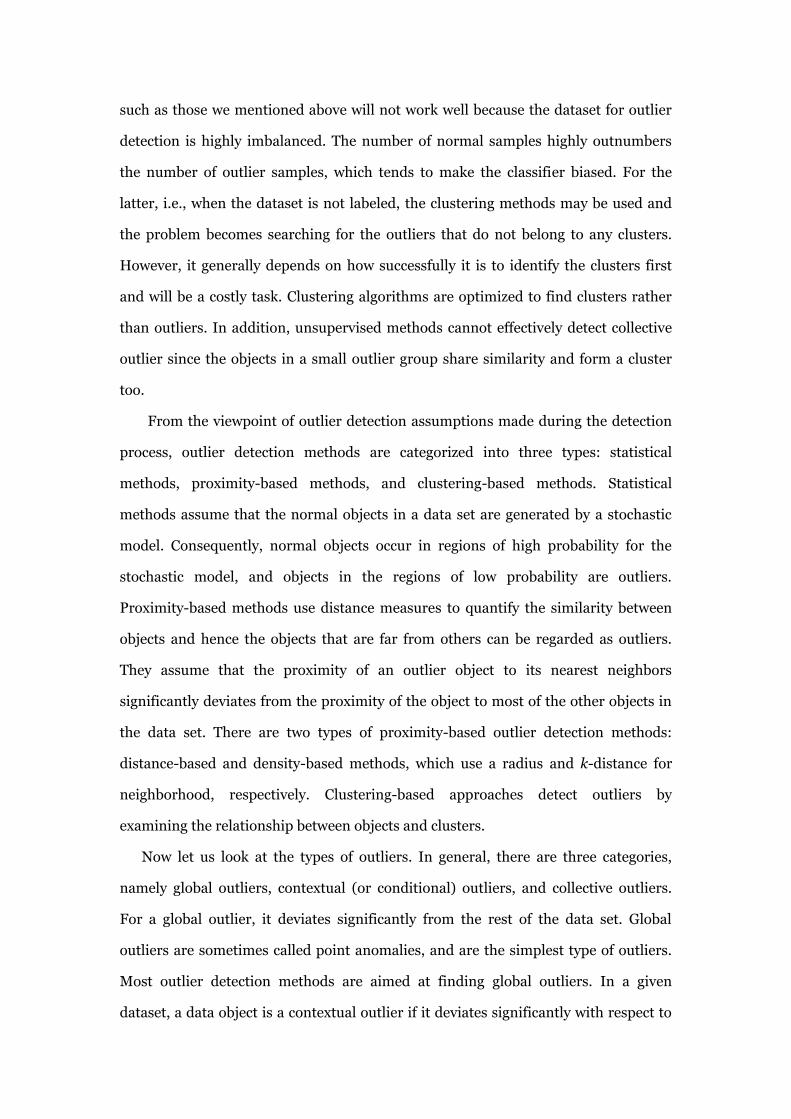
group of objects together form an abnormal pattern as in Fig. 1, that is the group

significantly differentiates itself from other objects with an unusual character, then

this group of objects as a whole is a collective outlier. In our case, the transactions

conducted for a seller together form a set of fabricated objects and hence is a

collective outlier. Neither on individual product nor on individual transaction can we

effectively detect the cheating behavior; the sellers of several fabricated transactions

will also do normal business and maintain multiple products and a shill may also

really shop for himself or herself other time.

For products in different genres, the probability of frauds will also change from

one to another. Our collection of transactions mainly related to one genre of product

and occurred during a period of time at a length of eight months. Attributes include

transaction date, product, product information, product quantity, seller, buyer etc. If

we consider that fabricated transactions had not come from real demands of random

customers, there could be high correlation among themselves. If we draw the

transactions as objects in a map, the fabricated ones are probably congest in a small

group and thus lead to high local abnormality (see Figure 1).

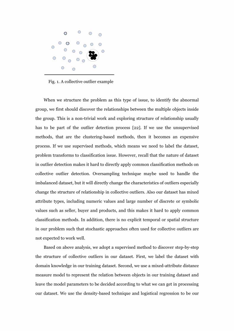
Fig. 1. A collective outlier example

When we structure the problem as this type of issue, to identify the abnormal

group, we first should discover the relationships between the multiple objects inside

the group. This is a non-trivial work and exploring structure of relationship usually

has to be part of the outlier detection process [22]. If we use the unsupervised

methods, that are the clustering-based methods, then it becomes an expensive

process. If we use supervised methods, which means we need to label the dataset,

problem transforms to classification issue. However, recall that the nature of dataset

in outlier detection makes it hard to directly apply common classification methods on

collective outlier detection. Oversampling technique maybe used to handle the

imbalanced dataset, but it will directly change the characteristics of outliers especially

change the structure of relationship in collective outliers. Also our dataset has mixed

attribute types, including numeric values and large number of discrete or symbolic

values such as seller, buyer and products, and this makes it hard to apply common

classification methods. In addition, there is no explicit temporal or spatial structure

in our problem such that stochastic approaches often used for collective outliers are

not expected to work well.

Based on above analysis, we adopt a supervised method to discover step-by-step

the structure of collective outliers in our dataset. First, we label the dataset with

domain knowledge in our training dataset. Second, we use a mixed-attribute distance

measure model to represent the relation between objects in our training dataset and

leave the model parameters to be decided according to what we can get in processing

our dataset. We use the density-based technique and logistical regression to be our

rest part of classifier to make use of distance measure model. We use the local

reachability density to test for possible distance model parameters on our training

dataset. And the logistic regression is to do further process on the result data from

local reachability density computation. The logistic regression model classifies

objects on their density space rather than on the raw feature space.

The local reachability density, however, will involve additional setting for

neighborhood. Therefore we select a set of expected values for neighborhood and,

together with distance model settings, investigate them with ability to separate

collective outlier from normal objects and select an empirical setting for all model

parameters. Thereafter we can directly compute object feature values into object

density values and classify them with logistic regression model.

After we have made the logistic regression model work at the best options, we

validate neighborhood settings and make modification if current value is not coming

with best final performance. Finally, we evaluate the method with our test dataset

and objectively evaluate our experiments. The main workflow is show in figure 2.

Data preprocess

Label datasets (supervised methods)

Training

datasetTest dataset

Model of distance

measurement

Density-based method

Logistic regression

Feature space

Density space

classifier

Relationship structure

Feature space

Neighborhood setting

Parameters investigation

training evaluation

Fig.2. workflow of data processing

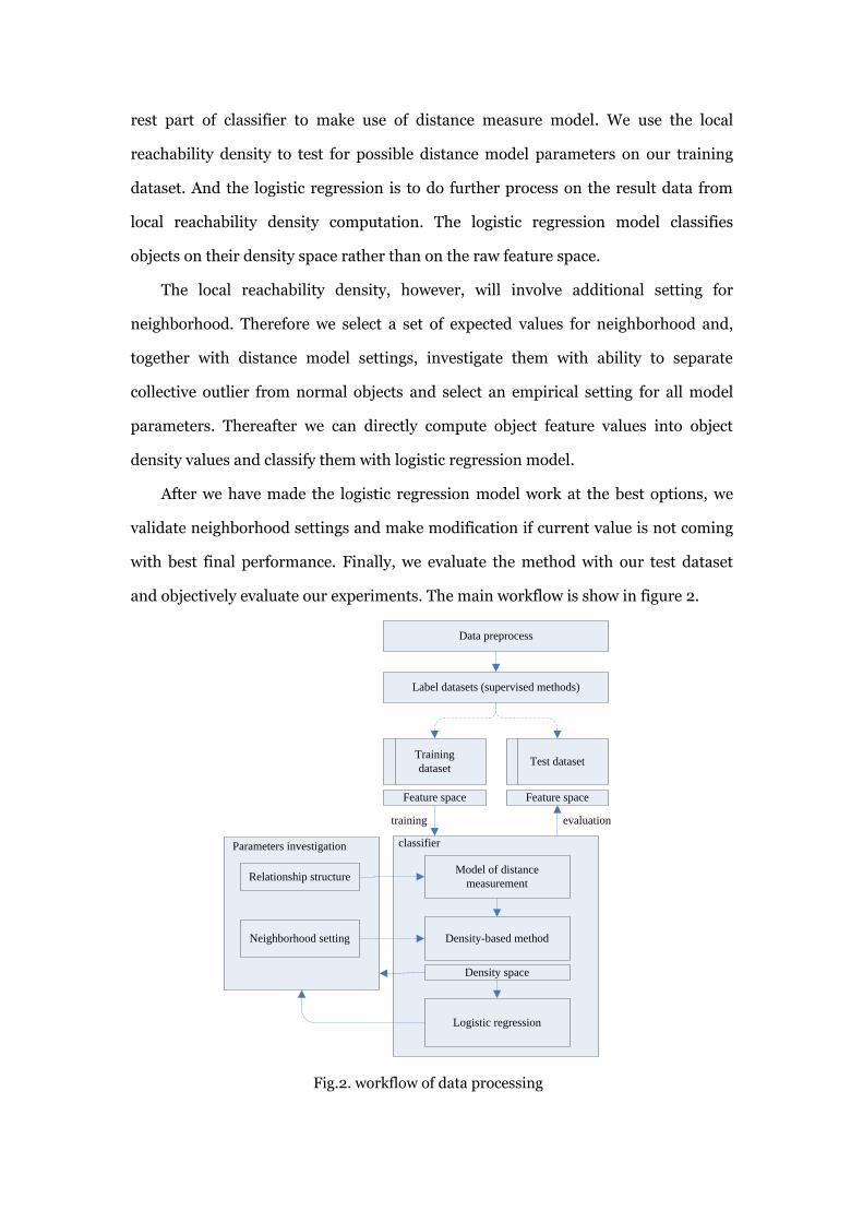
3.2 Model building

3.2.1 Distance measure model

To measure the distance or similarity between data objects, we should first

investigate the datasets containing the transactions information here. This requires

background knowledge for specific applications. From a list of features, we selected

some attributes that are computable in our model to fill our dataset as Table 1.

Table 1.

Attributes of the Transaction

Attribute Explanation Examples

id Transaction unique id 0,1,2…

seller The offer of this transaction Ivymagg**,maggie505**

location Location of seller Beijing,Shanghai

regTime Seller‟s registration time 2006-05-31

product Product unique id 10255280939

price Price of product 1550, 997.5

pstyle Style of product Black color, default style

quantity Quantity of products in

transaction

1, 2, 3…

buyer Buyer in this transaction d**u, g**n

date Occurred date of

transaction

2011-12-03

Instead of using Euclidean distance or standardized Euclidean distance, we use

weighted distance to measure mixed attribute types and define the distance measure

function as following:

Let T1, T2 be two transactions and let d(T1,T2) be the distance of T1,T2. For any

𝑇𝑖 , intuitively it is a row in the data set table, and formally noted with

𝑇𝑖 = (sr,loc,rtg,p,st,pr,q,br,dt)

where sr,loc,rgt,p,st,pr,q,br,dt are attributes for Seller, location, regTime, product,

pstyle, price, quantity, buyer and date respectively.

Now let A is the set of all attributes, 𝑎 is one attribute:

A = { sr,loc,rgt,p,st,pr,q,br,dt }, 𝑎 ∈ A,

then 𝑇𝑖(𝑎) is the value of attribute 𝑎.

We have the first definition of d(𝑇𝑖 , 𝑇𝑗):

d(𝑇𝑖 , 𝑇𝑗) = ∑ 𝑤𝑛

𝑎∈𝐴

∙ 𝐷 (𝑇𝑖(𝑎), 𝑇𝑗(𝑎)) + 𝑤0

where n is the index number of 𝑎 in A and D(x,y) is defined as:

D(x,y) = 𝐵(x, y) = {1, x ≠ y0, x = y

for a ∈ 𝐴1 = { sr,loc,p,st ,br }

D(x,y) = |(x − y) 𝑠𝑎⁄ | for a ∈ 𝐴2 = { dt,pr,rgt,q }, where 𝑠𝑎 is

the range of values of attribute 𝑎 and aim to normalization.

Then for a complete form of d(Ti, Tj) if we replace 𝑎 from above:

d(𝑇𝑖 , 𝑇𝑗) = ∑ 𝑤𝑛 ∙𝑎∈𝐴1𝐵 (𝑇𝑖(𝑎), 𝑇𝑗(𝑎)) + ∑ 𝑤𝑛 ∙𝑎∈𝐴2

|(𝑇𝑖(𝑎) − 𝑇𝑗(𝑎)) 𝑠𝑎⁄ | +𝑤0

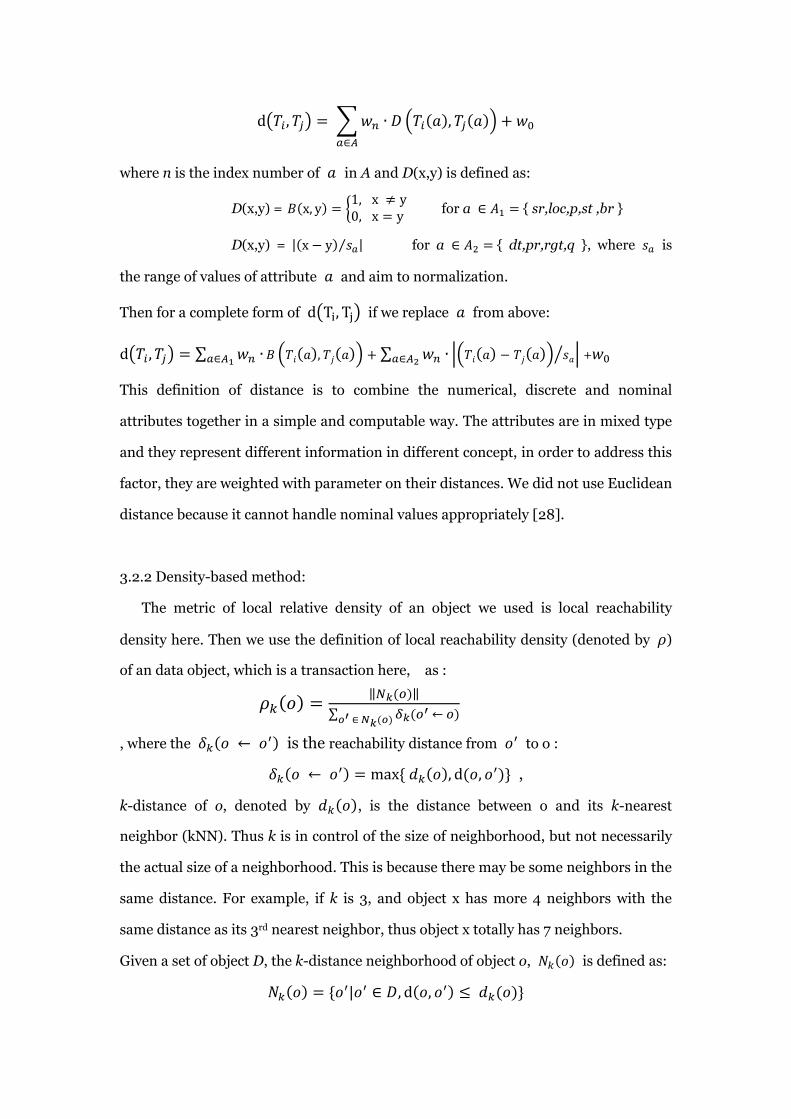
This definition of distance is to combine the numerical, discrete and nominal

attributes together in a simple and computable way. The attributes are in mixed type

and they represent different information in different concept, in order to address this

factor, they are weighted with parameter on their distances. We did not use Euclidean

distance because it cannot handle nominal values appropriately [28].

3.2.2 Density-based method:

The metric of local relative density of an object we used is local reachability

density here. Then we use the definition of local reachability density (denoted by 𝜌)

of an data object, which is a transaction here, as :

𝜌𝑘(𝑜) =‖𝑁𝑘(𝑜)‖

∑ 𝛿𝑘(𝑜′ ← 𝑜)𝑜′ ∈ 𝑁𝑘(𝑜)

, where the 𝛿𝑘(𝑜 ← 𝑜′) is the reachability distance from 𝑜′ to o :

𝛿𝑘(𝑜 ← 𝑜′) = max * 𝑑𝑘(𝑜), d(𝑜, 𝑜′)+ ,

k-distance of o, denoted by 𝑑𝑘(𝑜), is the distance between o and its k-nearest

neighbor (kNN). Thus k is in control of the size of neighborhood, but not necessarily

the actual size of a neighborhood. This is because there may be some neighbors in the

same distance. For example, if k is 3, and object x has more 4 neighbors with the

same distance as its 3rd nearest neighbor, thus object x totally has 7 neighbors.

Given a set of object D, the k-distance neighborhood of object o, 𝑁𝑘(𝑜) is defined as:

𝑁𝑘(𝑜) = *𝑜′|𝑜′ ∈ 𝐷, d(𝑜, 𝑜′) ≤ 𝑑𝑘(𝑜)+

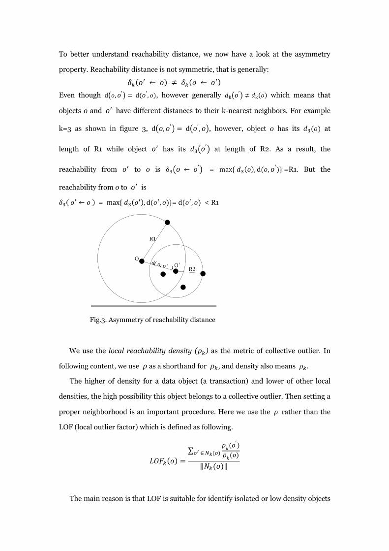
To better understand reachability distance, we now have a look at the asymmetry

property. Reachability distance is not symmetric, that is generally:

𝛿𝑘(𝑜′ ← 𝑜) ≠ 𝛿𝑘(𝑜 ← 𝑜′)

Even though d(𝑜, 𝑜′) = d(𝑜′, 𝑜), however generally 𝑑k(𝑜′) ≠ 𝑑k(𝑜) which means that

objects o and 𝑜′ have different distances to their k-nearest neighbors. For example

k=3 as shown in figure 3, d(𝑜, 𝑜′) = d(𝑜′, 𝑜), however, object o has its 𝑑3(𝑜) at

length of R1 while object 𝑜′ has its 𝑑3(𝑜′) at length of R2. As a result, the

reachability from 𝑜′ to o is δ3(𝑜 ← 𝑜′) = max * 𝑑3(𝑜), d(𝑜, 𝑜′)+ =R1. But the

reachability from o to 𝑜′ is

𝛿3( 𝑜′ ← 𝑜 ) = max * 𝑑3(𝑜′), d(𝑜′, 𝑜)+= d(𝑜′, 𝑜) < R1

O

O′d( o, o′)

R1

R2

Fig.3. Asymmetry of reachability distance

We use the local reachability density (𝜌𝑘) as the metric of collective outlier. In

following content, we use 𝜌 as a shorthand for 𝜌𝑘, and density also means 𝜌𝑘.

The higher of density for a data object (a transaction) and lower of other local

densities, the high possibility this object belongs to a collective outlier. Then setting a

proper neighborhood is an important procedure. Here we use the 𝜌 rather than the

LOF (local outlier factor) which is defined as following.

𝐿𝑂𝐹𝑘(𝑜) =

∑𝜌

𝑘(𝑜′)

𝜌𝑘

(𝑜)𝑜′ ∈ 𝑁𝑘(𝑜)

‖𝑁𝑘(𝑜)‖

The main reason is that LOF is suitable for identify isolated or low density objects

that too isolated to be included in any groups. So are other similar factors like LOF′

or LOF′′ [26]. Since we are identifying the collective outliers, we are actually

distinguishing minor groups with high local density. And different from normal

classification, we switch the feature space to density space thereafter the correlation

between objects could be measured based on density.

3.2.3 Logistic regression

To separate a minority from clusters, we set a cut-off for the density and the

minor objects (transactions) that on one side of the cut-off will be considered as the

expected ones. We employ the Logistic regression to classify densities into two classes,

one is the majority and the other is minority. Let Yi=1 if the transaction is fabricated:

𝑙𝑜𝑔 (𝑃(𝑌𝑖 = 1)

1 − 𝑃(𝑌𝑖 = 1)) = 𝛼 + 𝛽𝑋𝑖

Where 𝛼 is the intercept, 𝑋𝑖 (𝜌 of ith object) are the estimates, and the probability

for transaction to be fabricated is:

𝑃(𝑌𝑖 = 1) = 𝑒(𝛼+𝛽𝑋𝑖)

1+𝑒(𝛼+𝛽𝑋𝑖)

We use a default threshold (probability cut-off) of p=0.5 to decide the class for an

object.

4. Implementation and performance evaluation

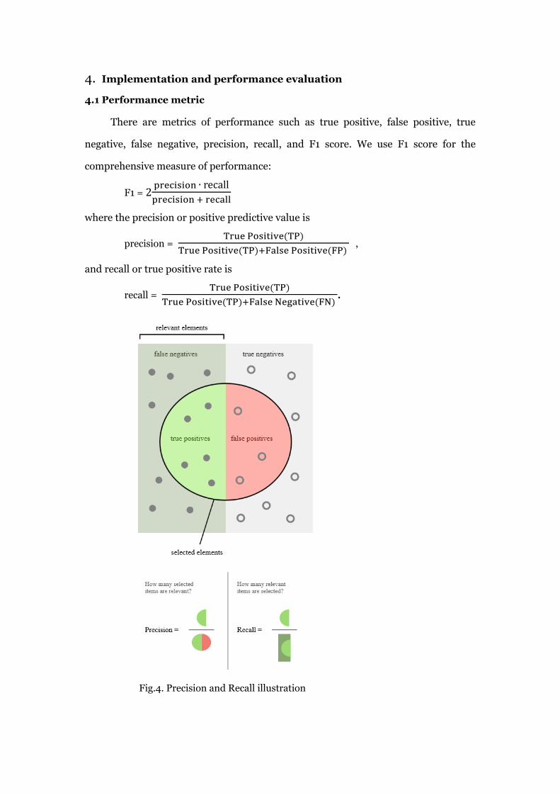
4.1 Performance metric

There are metrics of performance such as true positive, false positive, true

negative, false negative, precision, recall, and F1 score. We use F1 score for the

comprehensive measure of performance:

F1 = 2precision ∙ recall

precision + recall

where the precision or positive predictive value is

precision = True Positive(TP)

True Positive(TP)+False Positive(FP) ,

and recall or true positive rate is

recall = True Positive(TP)

True Positive(TP)+False Negative(FN) .

Fig.4. Precision and Recall illustration

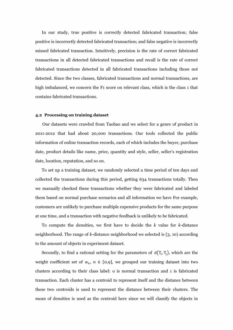
In our study, true positive is correctly detected fabricated transaction; false

positive is incorrectly detected fabricated transaction; and false negative is incorrectly

missed fabricated transaction. Intuitively, precision is the rate of correct fabricated

transactions in all detected fabricated transactions and recall is the rate of correct

fabricated transactions detected in all fabricated transactions including those not

detected. Since the two classes, fabricated transactions and normal transactions, are

high imbalanced, we concern the F1 score on relevant class, which is the class 1 that

contains fabricated transactions.

4.2 Processing on training dataset

Our datasets were crawled from Taobao and we select for a genre of product in

2011-2012 that had about 20,000 transactions. Our tools collected the public

information of online transaction records, each of which includes the buyer, purchase

date, product details like name, price, quantity and style, seller, seller‟s registration

date, location, reputation, and so on.

To set up a training dataset, we randomly selected a time period of ten days and

collected the transactions during this period, getting 634 transactions totally. Then

we manually checked these transactions whether they were fabricated and labeled

them based on normal purchase scenarios and all information we have For example,

customers are unlikely to purchase multiple expensive products for the same purpose

at one time, and a transaction with negative feedback is unlikely to be fabricated.

To compute the densities, we first have to decide the k value for k-distance

neighborhood. The range of k-distance neighborhood we selected is [3, 10) according

to the amount of objects in experiment dataset.

Secondly, to find a rational setting for the parameters of d(Ti, Tj), which are the

weight coefficient set of 𝑤𝑛, n ∈ [0,9], we grouped our training dataset into two

clusters according to their class label: o is normal transaction and 1 is fabricated

transaction. Each cluster has a centroid to represent itself and the distance between

these two centroids is used to represent the distance between their clusters. The

mean of densities is used as the centroid here since we will classify the objects in

density space according to their density values.

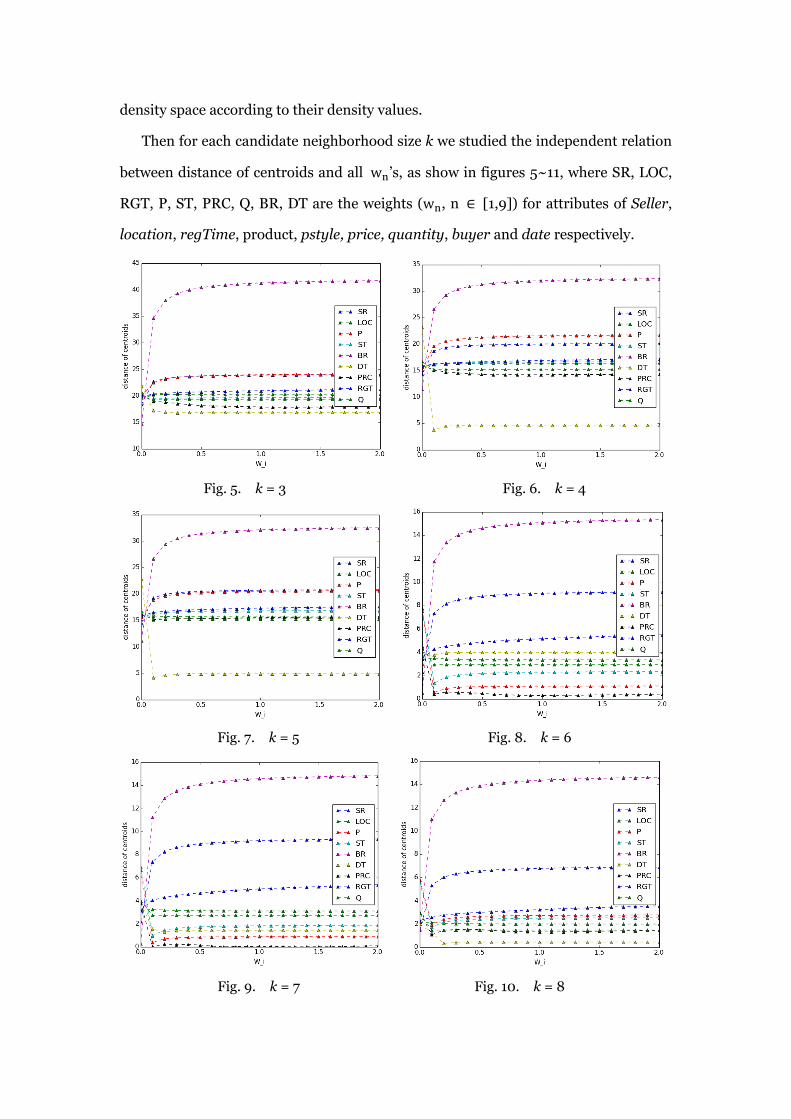
Then for each candidate neighborhood size k we studied the independent relation

between distance of centroids and all wn‟s, as show in figures 5~11, where SR, LOC,

RGT, P, ST, PRC, Q, BR, DT are the weights (wn, n ∈ [1,9]) for attributes of Seller,

location, regTime, product, pstyle, price, quantity, buyer and date respectively.

Fig. 5. k = 3 Fig. 6. k = 4

Fig. 7. k = 5 Fig. 8. k = 6

Fig. 9. k = 7 Fig. 10. k = 8

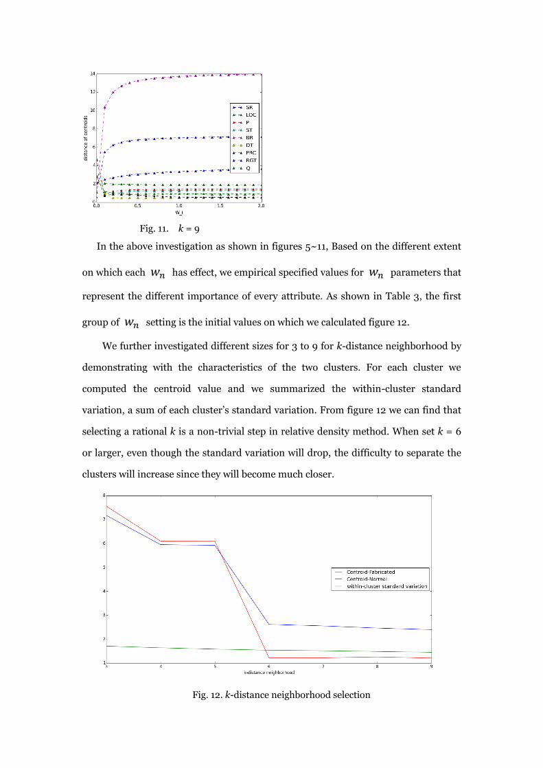
Fig. 11. k = 9

In the above investigation as shown in figures 5~11, Based on the different extent

on which each 𝑤𝑛 has effect, we empirical specified values for 𝑤𝑛 parameters that

represent the different importance of every attribute. As shown in Table 3, the first

group of 𝑤𝑛 setting is the initial values on which we calculated figure 12.

We further investigated different sizes for 3 to 9 for k-distance neighborhood by

demonstrating with the characteristics of the two clusters. For each cluster we

computed the centroid value and we summarized the within-cluster standard

variation, a sum of each cluster‟s standard variation. From figure 12 we can find that

selecting a rational k is a non-trivial step in relative density method. When set k = 6

or larger, even though the standard variation will drop, the difficulty to separate the

clusters will increase since they will become much closer.

Fig. 12. k-distance neighborhood selection

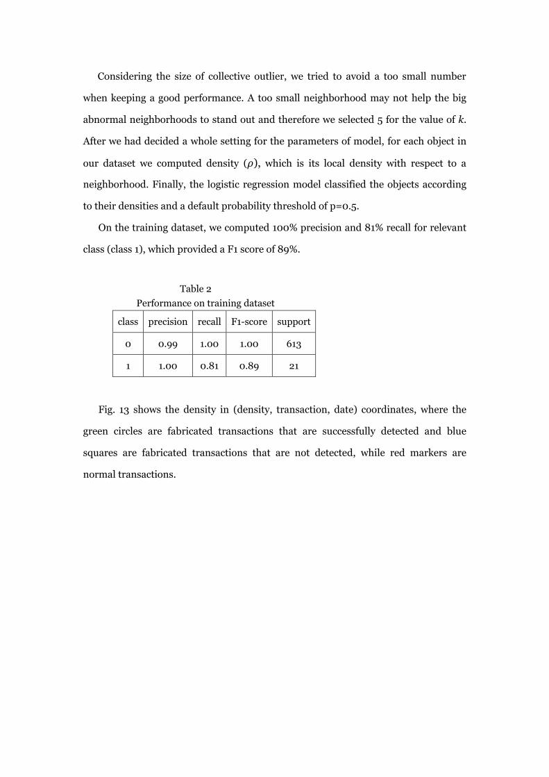
Considering the size of collective outlier, we tried to avoid a too small number

when keeping a good performance. A too small neighborhood may not help the big

abnormal neighborhoods to stand out and therefore we selected 5 for the value of k.

After we had decided a whole setting for the parameters of model, for each object in

our dataset we computed density (𝜌), which is its local density with respect to a

neighborhood. Finally, the logistic regression model classified the objects according

to their densities and a default probability threshold of p=0.5.

On the training dataset, we computed 100% precision and 81% recall for relevant

class (class 1), which provided a F1 score of 89%.

Table 2

Performance on training dataset

class precision recall F1-score support

0 0.99 1.00 1.00 613

1 1.00 0.81 0.89 21

Fig. 13 shows the density in (density, transaction, date) coordinates, where the

green circles are fabricated transactions that are successfully detected and blue

squares are fabricated transactions that are not detected, while red markers are

normal transactions.

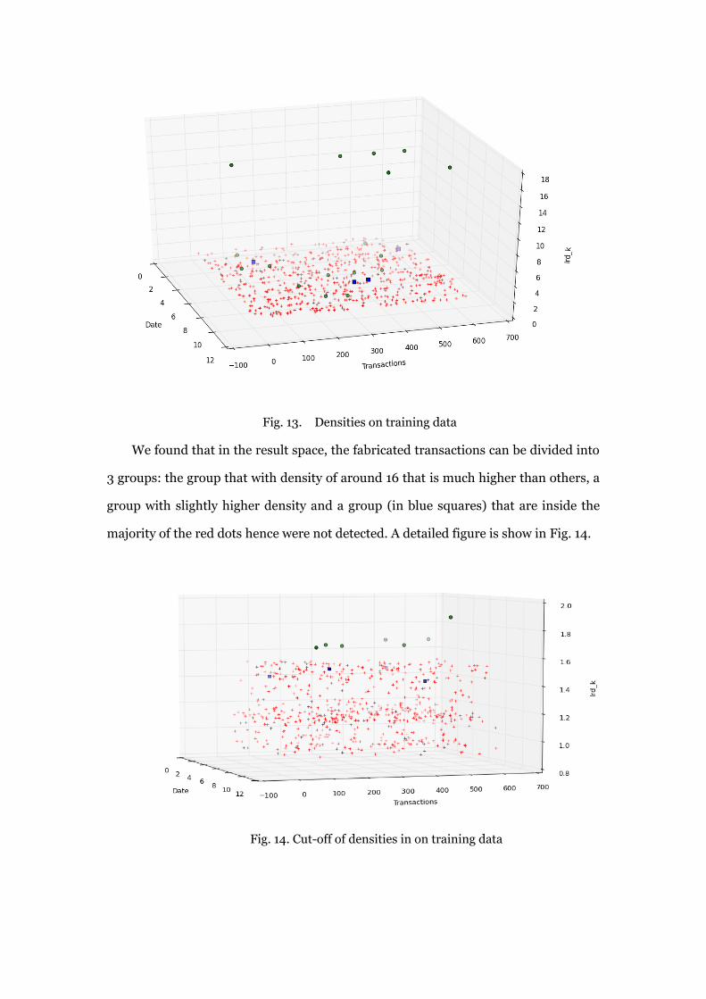
Fig. 13. Densities on training data

We found that in the result space, the fabricated transactions can be divided into

3 groups: the group that with density of around 16 that is much higher than others, a

group with slightly higher density and a group (in blue squares) that are inside the

majority of the red dots hence were not detected. A detailed figure is show in Fig. 14.

Fig. 14. Cut-off of densities in on training data

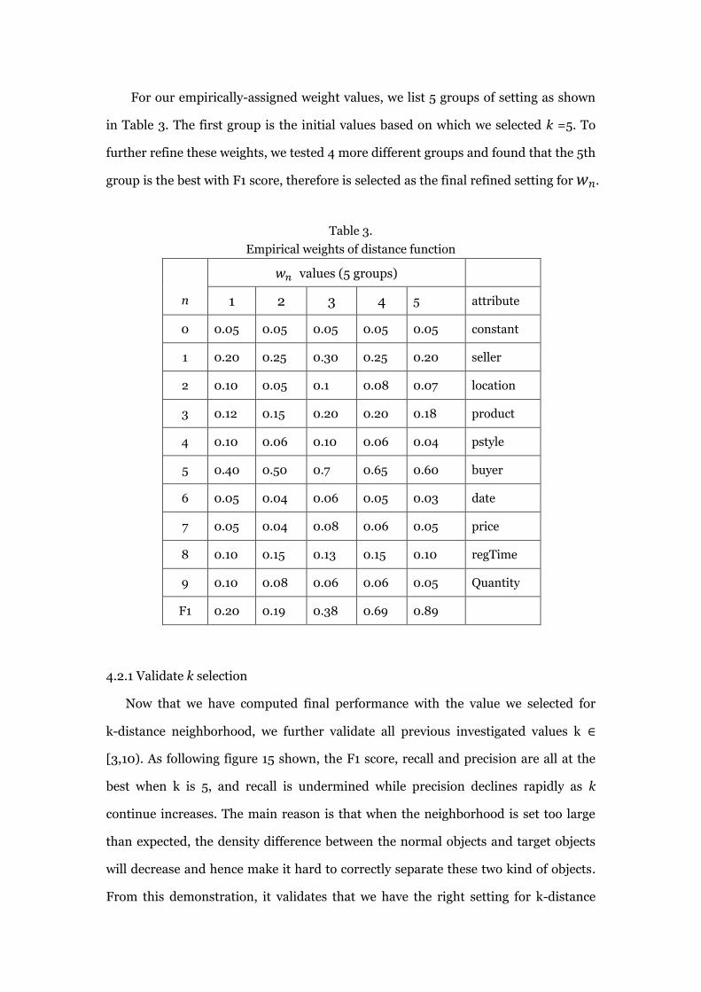
For our empirically-assigned weight values, we list 5 groups of setting as shown

in Table 3. The first group is the initial values based on which we selected k =5. To

further refine these weights, we tested 4 more different groups and found that the 5th

group is the best with F1 score, therefore is selected as the final refined setting for 𝑤𝑛.

Table 3.

Empirical weights of distance function

n

𝑤𝑛 values (5 groups)

1 2 3 4 5 attribute

0 0.05 0.05 0.05 0.05 0.05 constant

1 0.20 0.25 0.30 0.25 0.20 seller

2 0.10 0.05 0.1 0.08 0.07 location

3 0.12 0.15 0.20 0.20 0.18 product

4 0.10 0.06 0.10 0.06 0.04 pstyle

5 0.40 0.50 0.7 0.65 0.60 buyer

6 0.05 0.04 0.06 0.05 0.03 date

7 0.05 0.04 0.08 0.06 0.05 price

8 0.10 0.15 0.13 0.15 0.10 regTime

9 0.10 0.08 0.06 0.06 0.05 Quantity

F1 0.20 0.19 0.38 0.69 0.89

4.2.1 Validate k selection

Now that we have computed final performance with the value we selected for

k-distance neighborhood, we further validate all previous investigated values k ∈

[3,10). As following figure 15 shown, the F1 score, recall and precision are all at the

best when k is 5, and recall is undermined while precision declines rapidly as k

continue increases. The main reason is that when the neighborhood is set too large

than expected, the density difference between the normal objects and target objects

will decrease and hence make it hard to correctly separate these two kind of objects.

From this demonstration, it validates that we have the right setting for k-distance

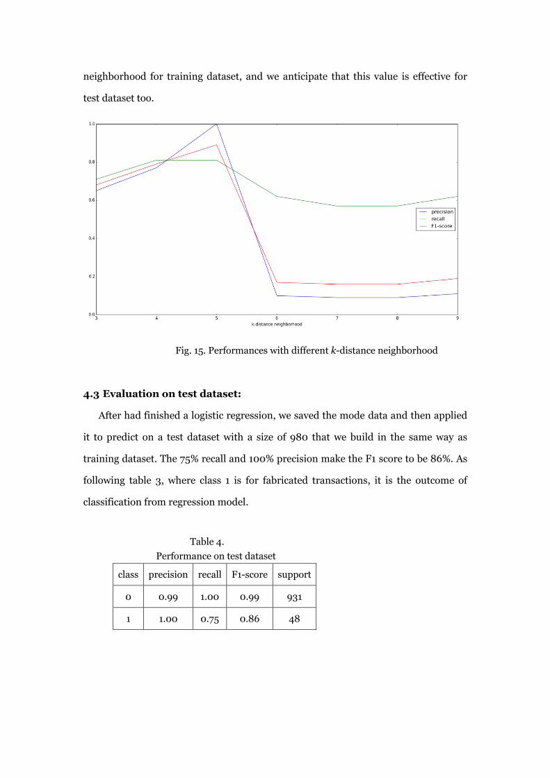
neighborhood for training dataset, and we anticipate that this value is effective for

test dataset too.

Fig. 15. Performances with different k-distance neighborhood

4.3 Evaluation on test dataset:

After had finished a logistic regression, we saved the mode data and then applied

it to predict on a test dataset with a size of 980 that we build in the same way as

training dataset. The 75% recall and 100% precision make the F1 score to be 86%. As

following table 3, where class 1 is for fabricated transactions, it is the outcome of

classification from regression model.

Table 4.

Performance on test dataset

class precision recall F1-score support

0 0.99 1.00 0.99 931

1 1.00 0.75 0.86 48

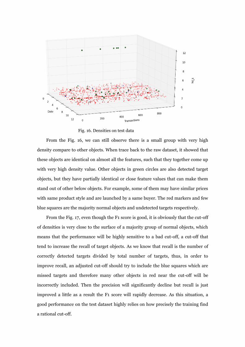
Fig. 16. Densities on test data

From the Fig. 16, we can still observe there is a small group with very high

density compare to other objects. When trace back to the raw dataset, it showed that

these objects are identical on almost all the features, such that they together come up

with very high density value. Other objects in green circles are also detected target

objects, but they have partially identical or close feature values that can make them

stand out of other below objects. For example, some of them may have similar prices

with same product style and are launched by a same buyer. The red markers and few

blue squares are the majority normal objects and undetected targets respectively.

From the Fig. 17, even though the F1 score is good, it is obviously that the cut-off

of densities is very close to the surface of a majority group of normal objects, which

means that the performance will be highly sensitive to a bad cut-off, a cut-off that

tend to increase the recall of target objects. As we know that recall is the number of

correctly detected targets divided by total number of targets, thus, in order to

improve recall, an adjusted cut-off should try to include the blue squares which are

missed targets and therefore many other objects in red near the cut-off will be

incorrectly included. Then the precision will significantly decline but recall is just

improved a little as a result the F1 score will rapidly decrease. As this situation, a

good performance on the test dataset highly relies on how precisely the training find

a rational cut-off.

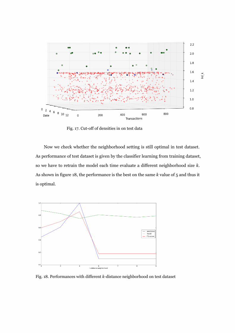
Fig. 17. Cut-off of densities in on test data

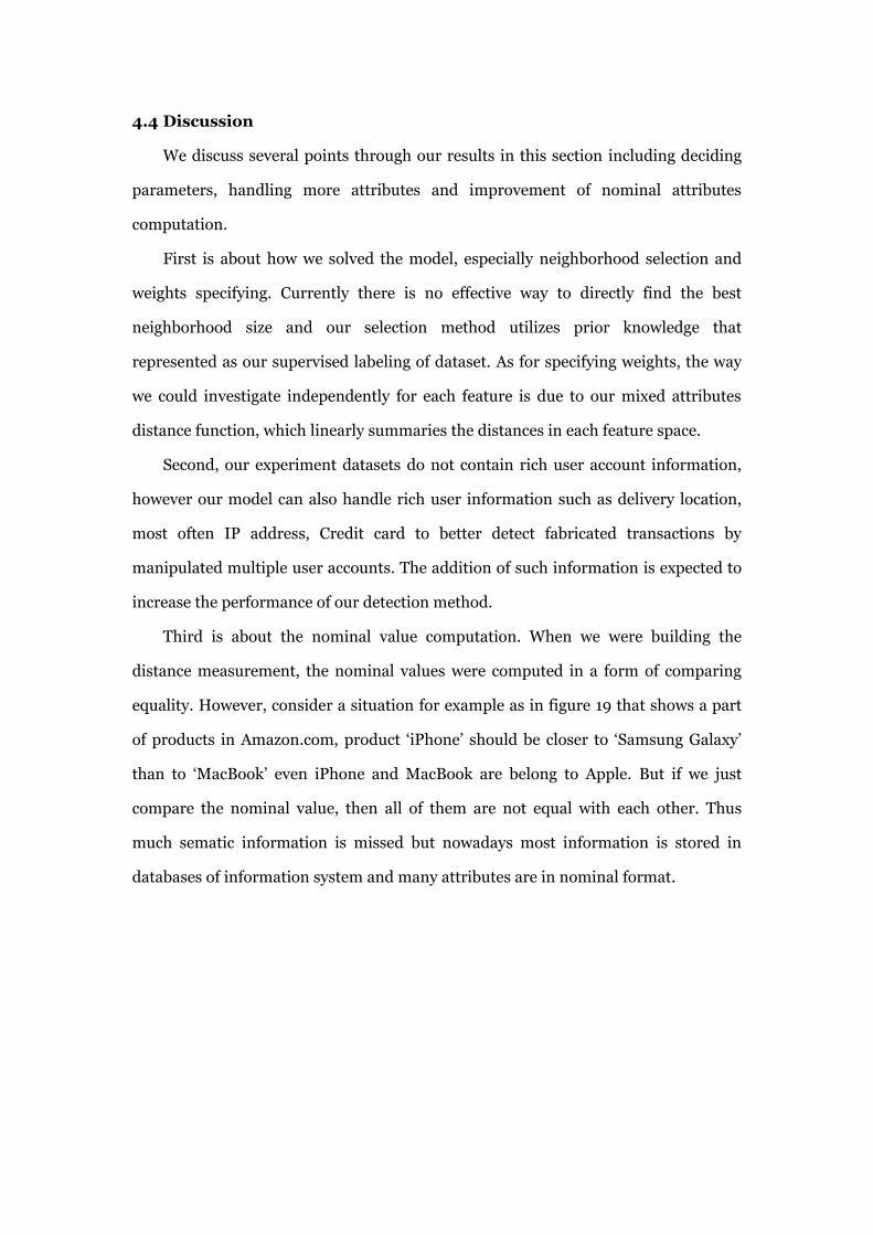
Now we check whether the neighborhood setting is still optimal in test dataset.

As performance of test dataset is given by the classifier learning from training dataset,

so we have to retrain the model each time evaluate a different neighborhood size k.

As shown in figure 18, the performance is the best on the same k value of 5 and thus it

is optimal.

Fig. 18. Performances with different k-distance neighborhood on test dataset

4.4 Discussion

We discuss several points through our results in this section including deciding

parameters, handling more attributes and improvement of nominal attributes

computation.

First is about how we solved the model, especially neighborhood selection and

weights specifying. Currently there is no effective way to directly find the best

neighborhood size and our selection method utilizes prior knowledge that

represented as our supervised labeling of dataset. As for specifying weights, the way

we could investigate independently for each feature is due to our mixed attributes

distance function, which linearly summaries the distances in each feature space.

Second, our experiment datasets do not contain rich user account information,

however our model can also handle rich user information such as delivery location,

most often IP address, Credit card to better detect fabricated transactions by

manipulated multiple user accounts. The addition of such information is expected to

increase the performance of our detection method.

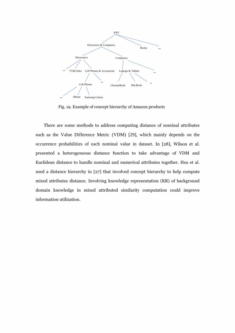
Third is about the nominal value computation. When we were building the

distance measurement, the nominal values were computed in a form of comparing

equality. However, consider a situation for example as in figure 19 that shows a part

of products in Amazon.com, product „iPhone‟ should be closer to „Samsung Galaxy‟

than to „MacBook‟ even iPhone and MacBook are belong to Apple. But if we just

compare the nominal value, then all of them are not equal with each other. Thus

much sematic information is missed but nowadays most information is stored in

databases of information system and many attributes are in nominal format.

ANY

Electronics & ComputersBooks

Electronics Computers

Cell Phones & Accessories...

...

TV&Video

...Cell Phones

iPhone Samsung Galaxy...

Laptops & Tablets ...

ChromeBook MacBook...

Fig. 19. Example of concept hierarchy of Amazon products

There are some methods to address computing distance of nominal attributes

such as the Value Difference Metric (VDM) [29], which mainly depends on the

occurrence probabilities of each nominal value in dataset. In [28], Wilson et al.

presented a heterogeneous distance function to take advantage of VDM and

Euclidean distance to handle nominal and numerical attributes together. Hsu et al.

used a distance hierarchy in [27] that involved concept hierarchy to help compute

mixed attributes distance. Involving knowledge representation (KR) of background

domain knowledge in mixed attributed similarity computation could improve

information utilization.

5. Conclusion

We have described a density-based collective outlier detection approach in

mixed-attribute datasets to detect fabricated online transactions. First we analyzed

the typical scenarios of how fabricated transactions take place in our applications in

C2C E-commerce. Based on the characteristics of these frauds and our analysis, we

modeled the problem to collective outlier detection. After preprocessed and labeled

the dataset, in the first place, we built a mixed attributes distance computation model

to measure the similarity of transactions and adopted density-based method to

convert the feature space to density space later.

When searching for a rational setting for all parameters, we chose a range of size

for k-distance neighborhood and a set of candidate neighborhood sizes. After

independently investigating the importance of each attribute on different candidate

neighborhood size, we set the weights of attributes in distance function. Then with

regarding the transactions as two clusters: normal and fabricated classes according to

the label, we decided the neighborhood size in terms of its ability to separate these

two clusters. In global densities, we use logistic regression method to classify the

transactions. At the end of learning on training dataset, we validated the

neighborhood size k with F1 scores.

Finally we objectively evaluated the method on test dataset. Even though there

are issues such as we listed in discussion that can be improved in future work, we

came up with a good result of our experiments.

REFERENCES

[1] L. Song, W. Zhang, S. S.Y. Liao, and R. C.W. Kwok, "A Critical Analysis Of The

State-Of-The-Art On Automated Detection Of Deceptive Behavior In Social Media." In PACIS,

p. 168. 2012.

[2] H. Xiong, Y. Ren, and P. Jia, "A Novel Classification Approach for C2C E-Commerce Fraud

Detection." International Journal of Digital Content Technology and its Applications 7, no. 1

(2013): 504.

[3] Y. Ku, Yuchi Chen, and C. Chiu, "A proposed data mining approach for internet auction

fraud detection." In Intelligence and Security Informatics, pp. 238-243. Springer Berlin

Heidelberg, 2007.

[4] W. Chang, and J. Chang, "An effective early fraud detection method for online

auctions." Electronic Commerce Research and Applications 11, no. 4 (2012): 346-360.

[5] A. Post, V. Shah, and A. Mislove, "Bazaar: Strengthening user reputations in online

marketplaces." In Proceedings of NSDI’11: 8th USENIX Symposium on Networked Systems

Design and Implementation, p. 183. 2011.

[6] F. Dong, S. M. Shatz, and H. Xu, "Combating online in-auction fraud: Clues, techniques and

challenges." Computer Science Review 3, no. 4 (2009): 245-258.

[7] D. Chau, S. Pandit, and C. Faloutsos, "Detecting fraudulent personalities in networks of

online auctioneers." In Knowledge Discovery in Databases: PKDD 2006, pp.103-114. Springer

Berlin Heidelberg, 2006.

[8] D. Chau, and C. Faloutsos, "Fraud detection in electronic auction." In European Web

Mining Forum at ECML/PKDD, pp. 87-97. 2005.

[9] N. Hu, L. Liu, and V. Sambamurthy, "Fraud detection in online consumer reviews." Decision

Support Systems 50, no. 3 (2011): 614-626.

[10] S. B. Caudill, M. Ayuso, and M. Guillén, "Fraud detection using a multinomial logit model

with missing information." Journal of Risk and Insurance 72, no. 4 (2005): 539-550.

[11] A. Mukherjee, V. Venkataraman, B. Liu, and N. Glance, Fake review detection:

Classification and analysis of real and pseudo reviews. UIC-CS-03-2013. Technical Report,

2013.

[12] J. Hayhurst, and D. P. Mundy, "Using Location as a Fraud Indicator for eCommerce

Transactions."

[13] J. Deng, L. Fu, and Y. Yi, "ZLOC: Detection of Zombie Users in Online Social Networks

Using Location Information."

[14] X. Wu, Z. Feng, W. Fan, J. Gao, and Y. Yu, "Detecting marionette microblog users for

improved information credibility." In Machine Learning and Knowledge Discovery in Databases,

pp. 483-498. Springer Berlin Heidelberg, 2013.

[15] J. Deng, X. Gao, C. Wang, “Using Bi-level Penalized Logistic Classifier to Detect Zombie

Accounts in Online Social Networks,” University of North Carolina at Greensboro, Jilin

University, 2015.

[16] K. Lee, J. Caverlee, and S. Webb, "Uncovering social spammers: social honeypots+

machine learning." In Proceedings of the 33rd international ACM SIGIR conference on

Research and development in information retrieval, pp. 435-442. ACM, 2010.

[17] F. Benevenuto, G. Magno, T. Rodrigues, and V. Almeida, "Detecting spammers on twitter."

In Collaboration, electronic messaging, anti-abuse and spam conference (CEAS), vol. 6, p. 12.

2010.

[18] M. Mccord, and M. Chua, "Spam detection on twitter using traditional classifiers."

In Autonomic and trusted computing, pp. 175-186. Springer Berlin Heidelberg, 2011.

[19] A. Wang, "Don't follow me: Spam detection in twitter," In Security and Cryptography

(SECRYPT), Proceedings of the 2010 International Conference on, pp. 1-10. IEEE, 2010.

[20] X. Jin, C. Lin, J. Luo, and J. Han, "A data mining-based spam detection system for social

media networks." Proceedings of the VLDB Endowment 4, no. 12 (2011): 1458-1461.

[21] V. Bewick, L. Cheek, and J. Ball, "Statistics review 14: Logistic regression." Crit Care 9, no.

1 (2005): 112-118.

[22] J. Han, M. Kamber, and J. Pei, Data mining: concepts and techniques. Elsevier, 2011. pp.

543-576.

[23] M. M. Breunig, H. Kriegel, R. T. Ng, and J. Sander, "LOF: identifying density-based local

outliers." In ACM sigmod record, vol. 29, no. 2, pp. 93-104. ACM, 2000.

[24] L. Duan, L. Xu, Y. Liu, and J. Lee, "Cluster-based outlier detection."Annals of Operations

Research 168, no. 1 (2009): 151-168.

[25] V. Chandola, A. Banerjee, and V. Kumar. "Outlier detection: A survey." ACM Computing

Surveys (2007).

[26] A. L. Chiu, and A. W. Fu. "Enhancements on local outlier detection." In Database

Engineering and Applications Symposium, 2003. Proceedings. Seventh International, pp.

298-307. IEEE, 2003.

[27] C. Hsu, and Y. Huang. "Incremental clustering of mixed data based on distance hierarchy."

Expert Systems with Applications 35, no. 3 (2008): 1177-1185.

[28] D. R. Wilson, and T. R. Martinez. "Improved heterogeneous distance functions." Journal of

artificial intelligence research (1997): 1-34.

[29] C. Stanfill, and D. Waltz. "Toward memory-based reasoning." Communications of the ACM

29, no. 12 (1986): 1213-1228.