Mass transfer and heat ﬂux in the vicinity of the Corinth ...mdoan/articles/DoanCornetGJI2006b.pdf · Geophys. J. Int. (2000) 142, 000–000 Mass transfer and heat ﬂux in the

Geophys. J. Int. (2000) 142, 000–000

Mass transfer and heat flux in the vicinity of the Corinth

Rift (Western Greece) Part II constraints from thermal

data

M.L. Doan1 and F.H. Cornet1

1 Institut de Physique du Globe de Paris, Paris, France

SUMMARY

The AIG10 borehole, on the southern shore of the Corinth Rift, provides a unique oppor-

tunity for evaluating the regional heat flux. Various thermal profiles have been performed,

some of them one year after drilling, whereas thermal conductivity has been measured on

cuttings and cores. The resulting measured heat flow in the upper part of the well above

the Aigio Fault is in the range of 60 mW/m2. The constant water temperature that has

been observed throughout the karstic aquifer below the fault is interpreted as a thermal

convection, given the absence of large regional water flow, demonstrated in Part I of this

paper. From experimental and theoretical characterization of porous media, the vertical

extent of the aquifer required for the onset of convection is evaluated to be 600 m. This

supports the previous proposition that this karstic aquifer extends within the Tripolitza

nappe rather than within the Pindos nappe. The thermal convection also fits with the

small temperature increase noticed close to the fault, a feature that cannot be explained

by simple fault mechanics.

2 M.L. Doan and F.H. Cornet

Key words: Heat Flux –Hydrogeology – Corinth Rift – Convection in porous media –

Thermal anomaly along faults

1 INTRODUCTION

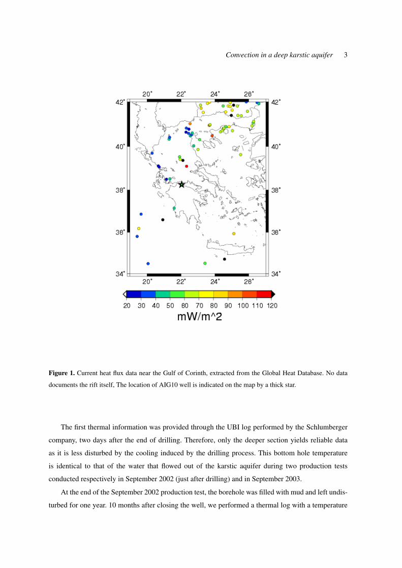
Global databases of the International Heat Flow Commission (http://www.heatflow.und.edu)

display only scarce and scattered data for Greece (figure 1) and give no information regarding the Gulf

of Corinth. The nearest published data documents the geothermal potential of the region of Loutraki,

near the eastern extremity of the gulf (Rominj et al.,1985 ). Interpolation profiles performed by (Hurtig

et al.,1992 ) completely ignore the rifting structure of the Gulf, whereas the region is not inventoried

by geothermal exploration studies (Fytikas et al.,2000 ).

Previous attempts to measure thermal flux within the Gulf (Bienfait and Koutsikos in 1995 (per-

sonal Communication)) failed because hydrological effects disturbed the thermal profiles, sometimes

resulting in negative thermal gradient. Indeed the high topography of the Corinth Gulf area is the

source of rapid downward cold flow through the shallow syn-rift sediments (Pizinno et al.,2004 ).

We present here results from heat flux evaluations obtained in two homogeneous sections of the

AIG10 well located above the Aigio Fault and discuss the absence of thermal gradient observed below

the fault down to the bottom of the well.

2 THERMAL MEASUREMENTS

The primary goal of the AIG10 borehole is to document the deformation processes of the Aigio fault.

Coring and various logs have been performed to constrain the geological and geophysical environment

of the fault (Comptes-Rendu geosciences, special issue, Cornet et al., 2004). The lithology crossed by

the borehole appears quite complex (figure 2). Below the syn-rift conglomerates, the Olonos-Pindos

sequence is observed, with tectonized layering of clays, radiolarite and limestone. This gross sequence

is complicated by thin stratifications at smaller scale. Indeed, the Pindos nappe is recognized as in-

tensely deformed and overthrusted by the Alpine compression (Rettenmaier et al.,2004 ). Limestone

encountered below the Aigio fault have a very steady pattern. They are heavily karstified and the hy-

drological properties of the footwall aquifer differ greatly from that of the upper units. The difference

in artesian pressure (0.5 MPa) between both aquifers indicates that the fault is somewhat impervious.

2.1 Thermal Profiles

Three successful thermal profiles were performed within the AIG10 well at different periods. Each

one documents a specific part of the borehole.

Convection in a deep karstic aquifer 3

Figure 1. Current heat flux data near the Gulf of Corinth, extracted from the Global Heat Database. No data

documents the rift itself, The location of AIG10 well is indicated on the map by a thick star.

The first thermal information was provided through the UBI log performed by the Schlumberger

company, two days after the end of drilling. Therefore, only the deeper section yields reliable data

as it is less disturbed by the cooling induced by the drilling process. This bottom hole temperature

is identical to that of the water that flowed out of the karstic aquifer during two production tests

conducted respectively in September 2002 (just after drilling) and in September 2003.

At the end of the September 2002 production test, the borehole was filled with mud and left undis-

turbed for one year. 10 months after closing the well, we performed a thermal log with a temperature


Figure 2. Schematic structural cross-section through Aigio fault. Note the variety of lithologies encountered by

the borehole.

reading recorded every 10 m with a resolution better than 0.01 ◦C. Unfortunately the lightness of the

probe prevented its lowering below 200 m.

In September 2003 personnel from GeoForshungsZentrum and Institut de Physique du Globe

used the Distributed Temperature Sensing (DTS) technology to obtain a thermal profile in an undis-

turbed environment. The principle of the measurement rests on the interpretation of temperature sen-

sitive Raman back-scattering and optical time-domain reflectometry within a fiber optics to provide

temperature-versus-depth data (Forster et al.,1997 ; Grosswig et al.,2001 ). By stacking data over time,

a precision of 0.3 ◦C may be obtained, with one data every meter. But the logging equipment could

not descend below the Aigio fault so that this thermal log reaches only a depth of 750m.

All three logs are compiled in figure 3. IPGP data on the 150m-200m interval yield a geothermal

gradient equal to G = 21.9 ± 0.20C/km that correlates well with the linear extrapolation of the

temperature between 700 and 750 m.

Thermal regime below the fault is only documented by the Schlumberger log. The bottom hole

temperature is similar to that measured near the Aigio fault, implicating a quasi-constant temperature

within the karstic aquifer in the footwall of the fault. This is confirmed by the steady 30 ± 1 ◦C


Figure 3. Thermal profiles performed within the AIG10 borehole.

water temperature measured during the various production tests, whereas extrapolation of the thermal

flux derived for a conductive regime would have produced water temperature increasing progressively

from 30 ◦C to 35 ◦C. This temperature reading is considered reliable given the 50 m3/hr flow rate,

over the three days of the 2002 production test. This uniform value is discussed in a latter section of

this article.

2.2 Measurement of Thermal Conductivity

2.2.1 Laboratory Sample Conductivity

In order to derive a thermal flux from these thermal profiles, we must evaluate the thermal conductiv-

ity of the material surrounding the borehole. Three kinds of rock samples have been considered for

constructing table 1.

We first used cuttings extracted at the 240 m, 480 m, 570 m, 595 m and 910 m drilling depths.

These depths were selected according to their petrological homogeneity. Synthetic samples were pre-

pared after washing and crushing the cuttings. Powders of known granularity were mixed with distilled


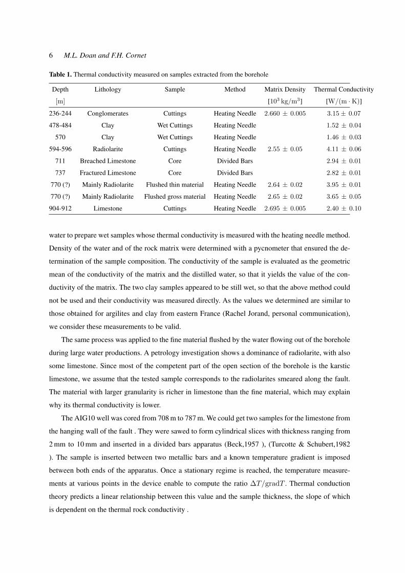
Table 1. Thermal conductivity measured on samples extracted from the borehole

Depth Lithology Sample Method Matrix Density Thermal Conductivity

[m] [103 kg/m3] [W/(m ·K)]

236-244 Conglomerates Cuttings Heating Needle 2.660 ± 0.005 3.15± 0.07

478-484 Clay Wet Cuttings Heating Needle 1.52 ± 0.04

570 Clay Wet Cuttings Heating Needle 1.46 ± 0.03

594-596 Radiolarite Cuttings Heating Needle 2.55 ± 0.05 4.11 ± 0.06

711 Breached Limestone Core Divided Bars 2.94 ± 0.01

737 Fractured Limestone Core Divided Bars 2.82 ± 0.01

770 (?) Mainly Radiolarite Flushed thin material Heating Needle 2.64 ± 0.02 3.95 ± 0.01

770 (?) Mainly Radiolarite Flushed gross material Heating Needle 2.65 ± 0.02 3.65 ± 0.05

904-912 Limestone Cuttings Heating Needle 2.695 ± 0.005 2.40 ± 0.10

water to prepare wet samples whose thermal conductivity is measured with the heating needle method.

Density of the water and of the rock matrix were determined with a pycnometer that ensured the de-

termination of the sample composition. The conductivity of the sample is evaluated as the geometric

mean of the conductivity of the matrix and the distilled water, so that it yields the value of the con-

ductivity of the matrix. The two clay samples appeared to be still wet, so that the above method could

not be used and their conductivity was measured directly. As the values we determined are similar to

those obtained for argilites and clay from eastern France (Rachel Jorand, personal communication),

we consider these measurements to be valid.

The same process was applied to the fine material flushed by the water flowing out of the borehole

during large water productions. A petrology investigation shows a dominance of radiolarite, with also

some limestone. Since most of the competent part of the open section of the borehole is the karstic

limestone, we assume that the tested sample corresponds to the radiolarites smeared along the fault.

The material with larger granularity is richer in limestone than the fine material, which may explain

why its thermal conductivity is lower.

The AIG10 well was cored from 708 m to 787 m. We could get two samples for the limestone from

the hanging wall of the fault . They were sawed to form cylindrical slices with thickness ranging from

2 mm to 10 mm and inserted in a divided bars apparatus (Beck,1957 ), (Turcotte & Schubert,1982

). The sample is inserted between two metallic bars and a known temperature gradient is imposed

between both ends of the apparatus. Once a stationary regime is reached, the temperature measure-

ments at various points in the device enable to compute the ratio ∆T/gradT . Thermal conduction

theory predicts a linear relationship between this value and the sample thickness, the slope of which

is dependent on the thermal rock conductivity .


2.2.2 Extrapolation to field conditions

So far, we have evaluated the thermal conductivities only for the matrix of representative small rock

samples. Extrapolation to the rock formation of the Pindos nappe requires some averaging. Rather

than proposing a continuous heat flux profile, we concentrate here on depths intervals where rocks

are fairly homogeneous, namely the upper conglomerates between 150 and 200 m and the limestone

formation just above the fault, between 710 and 750 m.

Further, in order to get the effective downhole conductivity value from laboratory measurements,

we must assess the in-situ porosity. Since this information is not available for depths intervals of in-

terest, some assumptions must be formulated.

The thermal conductivity of water is Kw = 0.6 W/K/m. Its presence within the pore space there-

fore decreases the effective rock conductivity Keff . In the absence of a precise knowledge of the pore

geometry, we use the classical geometrical averaging for the conductivities of both water Kw and rock

Kr, respectively over the volume of water Vw and that of rock Vr:

Keff = KVr

Vtotr × K

VwVtotw (1)

The quaternary conglomerate formation is expected to be largely porous and permeable. However,

the hydraulic test performed by (Giurgea et al.,2004 ) yields a moderate hydraulic conductivity C =

2.7 10−5 m/s. This suggests that the cobbles in the conglomerates are cemented. The drilling reports

do not mention the presence of any specific cement. Supposing that the filling material is similar to

that constituting the cobbles, we assimilate their conductivity to that measured at 240 m. We take a

small porosity, equal to about 5%.

Below 700 m, the DSI sonic log run by Schlumberger provides some information. The porosity

obtained with Schlumberger standard interpretation program is very noisy, with some negative values.

Yet it provides an estimate of a mean value and of its confidence level.

The conductivity determination method used for clay sample provides only a minimum order of

magnitude. The clay was manually compacted and inserted inside the pots used with the heating nee-

dle probe method. Thus the risk is high to let an important air volume inside the tested sample. This

would create a bias towards low conductivity values. To compensate this effect, we used the upper

value of the clay and a large uncertainty interval as shown in table 2, which compiles all estimations

of the effective thermal conductivity for the rock formation intersected by the borehole.


Matrix Porosity Effective

Rock Conductivity Porosity Conductivity

(W/(m ·K))) (%) (W/(m ·K))

Conglomerates 3.15 ± 0.07 5 ± 3 2.9 ± 0.3

Clay 1.5 ± 0.1 0 1.75 ± 0.25

Radiolarite 4.0 ± 0.1 3 ± 2 3.8 ± 0.2

Platy Limestone 2.9 ± 0.1 5 ± 3 2.7 ± 0.2

Deep Limestone 2.4 ± 0.1 7.5 ± 2.5 2.15 ± 0.15

Table 2. Estimation of the in-situ conductivities.

2.3 Heat Flow

To compute the heat flow, the temperature gradient is combined with the thermal conductivities.

On the upper section of the conglomerate, we retrieve a thermal gradient of G = 21.9± 0.20C/km

from the IPGP log. If we exploit the results of table 2, we obtain a heat flow comprised between

56mW/m2 and 70 mW/m2.

Similarly, the thermal log of GFZ is linear in most of the platy limestone section, as shown in the

close-up of figure 7. The thermal gradient is then G = 21.7 ± 0.20C/km. We then obtain a heat flow

value of 58.6 ± 4 mW/m2.

These value are consistent with the value of 55 mW/m2 obtained with a precise conductivity

profile by Postdam GeoForschungsZentrum (Forster,2006, personal communication).

The heat flow measured is then uniform within the platty limestone down to 740 m. There is no

significant thermal anomaly induced by fluid flow in the hanging wall of the Aigio fault. However, the

absence of heat flow evaluation in the karst prevents the direct extrapolation of the value to greater

depths. As discussed in the following section, even a small flow in the karst can deeply decrease the

heat flow measured in the upper section in the well. It is the hydraulic regime determined by long term

monitoring (part I of this paper) that will enable us to conclude with this respect.

3 ADVECTIVE HORIZONTAL FLOW

We explore here after possible perturbations caused by horizontal fluid motion, before investigating

vertical flow in the next section.

The heat flow advected by a horizontal water flow vx on a thickness H is

∆q = H vx ρf Cpf∂ T

∂ x(2)

ρf = 1000 kg/m3 and Cpf = 4180 J/(kg ×K) are respectively the volumetric mass and the heat

capacity of water. Supposing that the 30◦ hot water comes from the 2000 m-high mountains extending


10 km south to the site, we get an overestimate of ∂ T∂ x = 30/1 104 = 3 m◦C/m. The maximum hori-

zontal water velocity within the platy limestone just above the fault is estimated from both a small scale

production tests run during drilling and from the long term wellhead pressure monitoring described

in part II of this paper. It is found to be smaller than vx = 10−8 m/s (Doan & Cornet,2006 ). Hence

the maximum possible heat flux perturbation generated by water flow in the platy limestone remains

smaller than 2.0 mW/m2.The long term wellhead pressure monitoring provides also means to show

that the maximum horizontal water velocity in the karstic aquifer is smaller than vx = 10−10 m/s.

Given that the thickness of the aquifer is at most that of the Tripolitza limestone (2000 m), the

maximum heat flow advected through the karst is given by equation 2. Supposing also that the fluid

experienced a temperature variation of 30◦C in 10 km, the maximal heat flow disturbance is only

0.3 mW/m2. Hence the heat flux values derived from the upper thermal data is not expected to be

disturbed significantly by the local hydrological setting and sustains a regional significance.

We conclude that no thermal anomaly is detected in the southern shore of the Gulf of Corinth,

despite the existence of the system of active faulting.

4 ADVECTIVE VERTICAL FLOW

An intriguing feature of figure 3 is the absence of temperature variation in the lower karst aquifer. This

uniform temperature is comforted by the production test of September 2002, when the temperature of

the water flowing out of the borehole kept a constant 30◦C value for 3 days. The first explanation for

this absence of notable variation was to assume that the karst experienced large fluid flow (Micarelli

et al.,2005 ). However, the long term recording of the well head pressure already mentioned and

discussed in part I of this paper, demonstrates that this proposition is not valid. Thus, the onset of

convection in the karstic aquifer appears to be a more valid explanation.

4.1 Onset of convection

Convection in a fluid is triggered as soon as the Rayleigh number (Ra) reaches a threshold value. For

instance, the destabilization of a fluid mass with a dilatation coefficient α, a dynamic viscosity η and

a thermal diffusivity κ, placed between two parallel plates separated by a distance h that exhibits a

temperature difference ∆T occurs if:

Ra =α ρ g ∆Th3

κ η> 1708 (3)

An equivalent formulation has been developed for homogeneous porous media (Nield & Be-

jan,1992 ) :


Symbol Description Value

ρ Fluid volumic mass 103 kg/m3

g Gravity acceleration 10 m/s2

Cpf Fluid calorific capacity 4180 J/(K× kg)

η Fluid dynamic viscosity 10−3 Pa× s

λ Rock thermal conductivity 2.15 W/(K×m)

K Karst permeability 1.5 · 10−12 m2

α Thermal dilatation coefficient 3 · 10−4 K−1

Table 3. Parameters used in the characterization of the karst conduction.

Rap =α ρ g ∆T K H

λρ Cpf

η(4)

where K is the material permeability. The effective thermal diffusivity λρ Cpf

associates the rock ther-

mal conductivity λ and the thermal inertia of the fluid. The critical value Rac is smaller than in the

fluid case, and equals 4 π2 ≈ 40.

The onset of convection in the karst implies the inequality Ra > Rac which requires a minimal

value for the aquifer thickness given by

H >λ

ρ

√Rac η

α g qb K Cpf(5)

The meaning of the coefficients and the value we adopted are reported in table 3. The fluid properties

are extracted from tables for water at 30◦C (Lide,2005 ). Table 2 directly provides a value for λ = 2.15

The temperature difference ∆T is associated to the heat flux by the relationship qb = λW/(K×m).

The permeability of the karst could not be retrieved from direct production test because of its large

value, but it has been determined from tidal analysis (Doan & Cornet,2005 ).

Taking the values given in table 3, one gets the critical aquifer thickness H > 400 m. The UBI

sonic log of figure 4 shows that the karst spans the 230 m bottom section of the borehole. The uni-

formity assumption plausibly does not hold for so thick an aquifer and a progressive decrease of

permeability with depth is more likely. This decrease of permeability with depth would only result

in increasing the real aquifer thickness. Such a vertical extension for the karst cannot develop within

the Pindos nappe, since its limestone layers are not as thick and have never been observed to host

karstic structures . Hence it is concluded that the limestone in the footwall of the fault belongs to the

Tripolitza nappe, as previously suggested by (Rettenmaier et al.,2004 ).

We have supposed here that the aquifer boundaries are horizontal. Convection occurs more easily

if the boundaries were tilted, as a temperature gradient is applied at its lateral boundary (De Marsily,1986

). To examine this uncertainty, we consider here after the convection efficiency.


Figure 4. Ultra Sonic Borehole Imaging (amplitude data) of the AIG10 borehole. The karst exhibits cavities of

metric size.


Figure 5. Notations employed to describe the convection efficiency. We also show a typical temperature profile

within a convective medium.

4.2 Efficiency of convection

4.2.1 Experimental relationships for porous media

Convection is a more efficient heat transfer mode than conduction. As the temperatures at the bottom

and at the top of the convective medium are imposed, one experimentally observes that the heat transfer

through convection is higher than that through conduction, as given by Qdiff = λ ∆tH . The ratio

between the convective heat flow and the conductive Qdiff is the Nusselt number. It is equal to or

larger than 1.

The mean temperature in the karst is the average of the two temperatures at its top and its bot-

tom boundaries. As we do not know their depths, these two temperatures are unknown. However we

can limit their range. The top temperature is estimated by extrapolation of the temperature profile of

figure 3. We also know the temperature inside the convection cell, so that the knowledge of the top

temperature constrains the temperature at the bottom boundary.

A typical vertical temperature profile is presented in figure 5. Strong temperature gradients are

confined within a transition layer, whereas the temperature is quasi uniform within the cell. Supposing

that the bottom and top transition layers are symmetric, one gets ∆T = Tt − Tb = 2 (Tmes − Tt).

It is then possible to estimate the temperature at the base of the karst and get for the Nusselt number

NuP :

NuP =q H

2 λ (Tt − Tmes)(6)

Experimental studies on convection in porous media have shown a correlation between the tem-

perature difference ∆T and the Nusselt number (Cheng,1978 ). Since then, the dispersion of the data

has been explained by inertial effects. (Bejan,2003 ) gives an experimental formula that summarizes

their data :

NuP =((

RaP

4 π2

)n

+(c√

PrP RaP

)n)1/n

(7)


where n = −1.65 and c = 1896. Equation 7 involves the Prandtl number PrP , which compares

thermal conduction to viscosity effect. In a fluid, it would be expressed as Prf = (η/ρ)/(λf/(ρCpf )).

In a porous medium, this quantity is regulated by the departure of the actual hydraulic regime from

Darcy equation :

PrP =η/ρ

λρ Cpf

H

b K(8)

Indeed, if the pores are too large or if the fluid velocity is too fast, the relationship between the fluid

flow rate and the pressure gradient is no more linear. One then have to use the Forchheimer equation :

−−−→grad(p) =η

K~v + b ρ v ~v (9)

If the b parameter is null, one retrieves the Darcy law. By analogy with studies on turbulent regime,

(Ward,1964 ) have reformulated equation 9 in terms of ”drag” coefficient.

f =∥∥∥−−−→grad(p)

∥∥∥ √K

ρ v2(10)

He experimentally demonstrated that f = 1/ReP + C, where ReP = ρ v√

K/η is the Reynold

number for the porous medium and C is a constant equal to 0.55. One deduces the result : C =√

K b.

Combining this result with equation 8, one gets a Prandtl number larger than 3 108 as H < 220 m.

(Nield & Bejan,1992 ) compare this number to the Rayleigh number. If Ra < Pr, convection is

dominated by Darcy law. If on the contrary Ra > Pr, convection is controlled by the non-linear term

of Forchheimer equation. The maximum value of RaP for the karst is about 3000, with the extreme

values for heat flow q = 200 mW/m2 and for aquifer thickness H = 2000 m. Darcy’s law therefore

controls water flow inside the karst.

4.2.2 Application to the Aigio well

Estimation of the aquifer height

Combining equations 6 and 7, the relationship between (Tt − Tmes), H and q is :

Tmes − Tt =qH2 λ

((α ρ2 g Cpf qK H2

4 π2 λ2 η

)n

+

c

√α ρ2 g C2

pf q√

K H3

C λ3

n−1/n

(11)

Only the parameters denoted with bold letters in equation 11 are unknown. The aquifer thickness is

thus linked to the temperature difference Tmes − T , which is bounded by the 150 m vertical offset

of the fault. The top of the karst zt cannot be distant by more than 150 m from the intersection of the

borehole and the fault. By extrapolating the thermal gradient of figure 7, we get an underestimate of


200 400 600 800 1000 1200 1400 1600 1800 20000

2

4

6

8

10

12

Aquifer thickness (m)

Tm

es−

Tt (

0 C)

0m

50m

100m

150m

770−zt

qb=70mW/m2

qb=100mW/m2

qb=200mW/m2

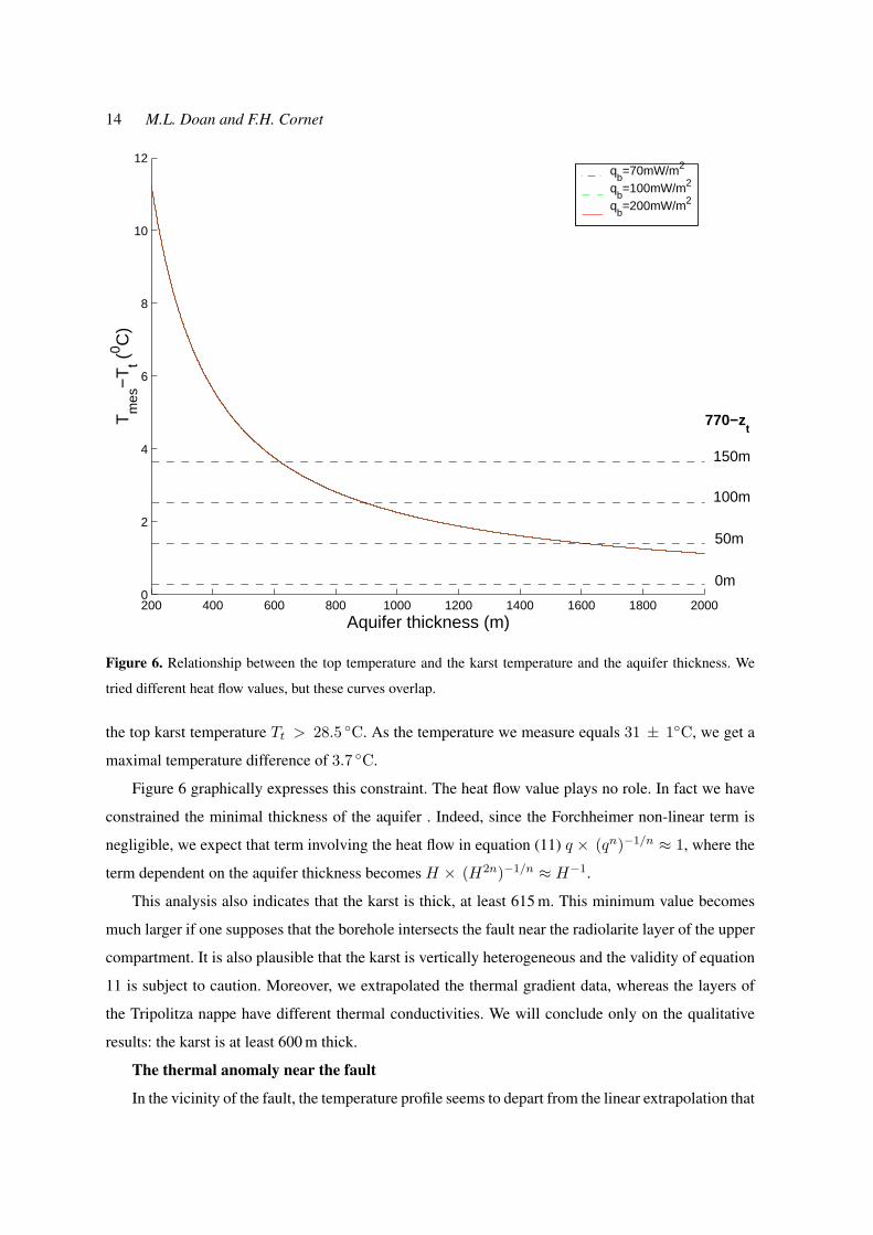
Figure 6. Relationship between the top temperature and the karst temperature and the aquifer thickness. We

tried different heat flow values, but these curves overlap.

the top karst temperature Tt > 28.5 ◦C. As the temperature we measure equals 31 ± 1◦C, we get a

maximal temperature difference of 3.7 ◦C.

Figure 6 graphically expresses this constraint. The heat flow value plays no role. In fact we have

constrained the minimal thickness of the aquifer . Indeed, since the Forchheimer non-linear term is

negligible, we expect that term involving the heat flow in equation (11) q × (qn)−1/n ≈ 1, where the

term dependent on the aquifer thickness becomes H × (H2n)−1/n ≈ H−1.

This analysis also indicates that the karst is thick, at least 615 m. This minimum value becomes

much larger if one supposes that the borehole intersects the fault near the radiolarite layer of the upper

compartment. It is also plausible that the karst is vertically heterogeneous and the validity of equation

11 is subject to caution. Moreover, we extrapolated the thermal gradient data, whereas the layers of

the Tripolitza nappe have different thermal conductivities. We will conclude only on the qualitative

results: the karst is at least 600 m thick.

The thermal anomaly near the fault

In the vicinity of the fault, the temperature profile seems to depart from the linear extrapolation that


fits the temperature in the platy limestone (bottom graph of figure 7). Is this increase in temperature

correlated to the fault movement ?

(Lachenbruch & Sass,1980 ) predicted the heat production rate induced by fault motion as Q =

vrel τ , where τ is the tangential stress applied on the fault and vrel the relative velocity. This expres-

sion is only an approximation since one cannot maintain both a constant stress and a constant fault

movement. For instance, if a constant load is applied, the heat would induce a softening of the fault

and an increase in slip velocity. This estimation is indeed only an overestimation as the fault velocity

increases with time. We suppose that the load is controlled by gravity, so that τ = ρ g z sin θ. The slip

velocity is determined from geological consideration. The age of the Aigio fault is about 50,000 yr

and its vertical offset is 150 m (Cornet et al.,2004b ). The slip velocity is therefore v = 3 mm/yr. At a

depth of 800 m, this gives a heat production rate equal to 0.6 mW/m2 only. The fault effect is therefore

negligible.

The temperature in a convective karst is quasi-uniform. This disturbs the temperature field in its

neighborhood. Is this disturbance large enough to explain the temperature anomaly near the fault ?

To illustrate this phenomenon, we conducted numerical simulation on two different configurations.

In the first case, the borehole intersects the fault near the radiolarite layer of the hanging wall. The

temperature field and its gradient are presented together with the expected temperature profile in the

well in the left graph of figure 7. A similar graph is also presented in the case when the borehole and

fault intersection lies near the radiolarites of the footwall.

We used the PDE Toolbox of Matlab software, with a geometry partly visible on figure 7. The

crust is taken as a 2D square, 30 km high and 2000 m thick. A constant heat flow is applied at the

bottom boundary, whereas the lateral boundaries have no-flow (Neumann) boundary conditions and

the incoming heat flux through the upper section is null. A zero-temperature is imposed at the surface.

The karst bottom boundaries has been set to 1500 m on both the hanging wall and the footwall. How-

ever, its top boundary position is different for the two compartments, to reflect the 150 m offset of the

Aigio fault. The effect of the convection in the karst is expressed by a thermal conductivity 50 times

larger than those in the surrounding media (set at 3 W/(K×m)).

One notices that in both cases, the expected thermal profile departs significantly from the linear

profile near the fault. But, the sign and the value of its curvature differ. On the right graph, the temper-

ature profile is deformed towards the greater temperatures in a close vicinity to the fault. In the other

case the departure to the linearity occurs at shallower depths and trends towards smaller temperatures.

This simulation has the disadvantage of involving several effects. First, the difference between

the temperature inside the karst and that in the platy limestone near the intersection of the borehole

and the fault is not taken into account. The curvature is expected to be positive if the karst is hotter


Deep radiolarite layer case

0 10 20 30 40 50 60−1500

−1000

−500

0

∆ T (0C)

Dep

th (

m)

conduction : k=3W/(K*m)convection : k=100W/(K*m)

Shallow radiolarite layer case

Figure 7. The borehole position relative to the karst influences the thermal profile. On the top of the figure, we

display the temperature field for to different positions of the intersection point between the borehole and the top

of the karst in the hanging wall. We also present the expected temperature profile along the borehole, in two

cases: when the thermal regime karst is controlled by conduction or by convection. In the last case, the thermal

efficiency convection is expressed by a higher equivalent thermal conductivity, arbitrarily set to 50 mW/m2. In

the conduction case, the temperature is modified within the karst, but also close to the karst for both geometries.

In the second geometry, the convection profile departs from the conduction profile, in a shape similar to the

thermal anomaly observed in the AIG10 borehole (bottom graph).


than the value derived from the thermal gradient in the upper layer. This is the main effect we wanted

to highlight. The geometry also alters the shape of the anomaly. Point effects are more important

near the edge of the karst. An additional effect is due to the simulation strategy. We impose the heat

flux to be accommodated between the top of the karst, which acts as a isotherm volume, and the

ground surface, whose temperature is imposed. The fault offset implies that the surface layers have

different temperature. The geothermal gradient therefore artificially differs in both compartment due

to geometrical effects.

In order to quantify further this effect, a more accurate understanding of the borehole configuration

is necessary. Unfortunately, the positions of most of the layers in the hanging wall and in the footwall

remain unknown. It is only concluded here that the models of karst convection are compatible with a

temperature anomaly with an amplitude comparable to that observed.

5 CONCLUSION

The Aigio AIG10 borehole is deep enough to conduct reliable thermal measurements so that the

corresponding heat flux determination is representative of the Corinth Rift area and is not hampered by

surface water flow. The low value, only 60±10 mW/m2, is surprising when considering the extensive

system of active faults observed in this rift. However it is consistent with geodetic and gravimetric data

that show that the Peloponnesus acts presently as a rigid block, and with seismic data that place the

Moho discontinuity at a depth of about 39 km.

With an extensive karst extending in the deepest layer encountered by the borehole, the Aigio well

is controlled by extensive hydrothermal coupling. This interpretation relies on results discussed in part

I of this paper that describes the long term pressure variations monitored in the well to conclude that

the thermal data are not affected by hydraulic flow in the karst.

In fact the karst is the site of thermal convection, a fact rarely observed in the field. This indi-

cates that the karst vertical extension is at least 600 m. This convection model also predicts a thermal

anomaly near its interface, here constituted by the borehole, which is indeed observed.

ACKNOWLEDGMENTS

We especially thank the Laboratoire des Systemes dynamiques of the Institut de Physique du Globe

de Paris for having accepted to share their expertise on heat flow measurement. We also thank Andrea

Forster, from GFZ institute for having accepted to share the temperature data near the Aigio fault. We

are grateful to Claude Jaupart and Ghislain de Marsily for their fruitful discussion. The CRL devel-

opment benefited from support from the Energy Environment and Sustainable Development program


of the European Commission (in particular contract nb EVR1-CT-2000-40005) and from the French

CNRS (GDR-Corinth).

REFERENCES

Avallone, A., Briole, P., Agatza-Balodimou, A., Billiri, H., Charade, O., Mitsakaki, C., Nercessian, A., Pa-

pazissi, K., Paradissis, D., & Veis, G., 2004. Analysis of eleven years of deformation measured by GPS in

the Corinth Rift Laboratory area, C.R.Geoscience, 336(4-5), 301–311.

Beck, A., 1957. A steady state method for the rapid measurement of the thermal conductivity of rocks, J. Sci.

Instrum., 34, 186–189.

Bejan, A., 2003. Porous media, in Heat transfer handbook, edited by A. Bejan & A. Kraus, chap. 15, Wiley &

sons.

Bernard, P., Lyon-Caen, H., Briole, P., Deschamps, A., Boudin, F., Makropoulos, K., Papadimitriou, P.,

Lemeille, F., Patau, G., Billiris, H., Paradisis, D., Papazissi, K., Castarde, H., Charade, O., Nercessian, A.,

Avallone, A., Pacchiani, F., Zaradnik, J.and Sacks, S., & Linde, A., 2005 (in press). Seismicity, deforma-

tion and seismic hazard in the western rift of Corinth : New insights fom the Corinth Rift Laboratory (crl),

Tectonophysics.

Briole, P., Rigo, A., Lyon-Caen, H., Ruegg, J. C., Papazissi, K., Mitsakaki, C., Balodimou, A., Veis, G.,

Hatzfeld, D., & Deschamps, A., 2000. Active deformation of the Corinth rift, Greece: Results from repeated

Global Positioning System surveys between 1990 and 1995, J. Geophys. Res., 105(B11), 25605–25625.

Cheng, P., 1978. Geothermal systems, Adv. Heat Transfer, 14, 1–105.

Cornet, F., Bernard, P., & Moretti, I., 2004. The Corinth Rift Laboratory, C.R.Geoscience, 336(4-5), 235–241.

Cornet, F., Doan, M., Moretti, I., & Borm, G., 2004. Drilling through the active Aigion Fault: the AIG10 well

observatory, C.R.Geoscience, 336(4-5), 395–406.

De Marsily, G., 1986. Quantitative Hydrogeology. Groundwater Hydrology for Engineers., Academic Press,

Inc.

Doan, M. & Cornet, F., 2005. Complete hydraulic characterization of a deep confined coastal aquifer through

tidal analysis, Submitted to J. Geophys. Res..

Doan, M. & Cornet, F., 2006. Mass transfer and heat flux in the vicinity of the Corinth Rift (Western Greece)

- part I constraints from long term pressure variations, Submitted to Geophys. J. Int..

Forster, A., Schrotter, J., & Merriam, D., 1997. Application of optical-fiber temperature logging – an example

in a sedimentary environnement, Geophysics.

Fytikas, M., Andritsos, N., Karydakis, G., Kolios, N., Mendrinos, D., & Papachristou, M., 2000. Geother-

mal exploration and development activities in Greece during 1995-1999, in Proceedings World Geothermal

Congress 2000, pp. 199–206, Kyushu-Tohoku, Japan.

Giurgea, V., Rettenmaier, D., Pizzino, L., Unkel, I., Hotzl, H., Forster, A., & Quattrocchi, F., 2004. Preliminary

hydrogeological interpretation of the Aigion area from the AIG10 borehole data, C.R.Geoscience, 336(4-5),

467–475.


Grosswig, S., Hurtig, E., Kuhn, K., & Rudolph, F., 2001. Distributed fibre-optic temperature sensing technique

(DTS) for surveying underground gas storage facilities, Oil Gas European Magazine.

Hurtig, E., Cermak, V., Haenel, R., & Zui, V., eds., 1992. Geothermal Atlas of Europe, Hermann Haack, Gotha.

Lachenbruch, A. & Sass, J., 1980. Heat flow and energetics of the San Andreas Fault Zone, J. Geophys. Res.,

85(B11), 6185–6222.

Le Pichon, X., Chamot-Rooke, N., Lallemant, S., Noomen, R., & Veis, G., 1995. Geodetic determination of

the kinematics of central greece with respect to europe: Implications for eastern mediterranean tectonics, J.

Geophys. Res., 100(B7), 12,675–12,690.

Lide, D., ed., 2005. CRC Handbook of Chemistry and Physics, CRC Press, 85th edn.

Lyon-Caen, H., Papadimitriou, P., Deschamp, A., Bernard, P., Makropoulos, K., Pacchiani, F., & G., P., 2004.

First results of the CRLN seismic network in the western Corinth Rift: evidence for old-fault reactivation,

C.R.Geoscience, 336(4-5), 343–351.

Micarelli, L., Moretti, I., Jaubert, M., & Moulouel, H., 2005. Fault hydraulic behavior, a multidisciplinary

approach through the normal faults of the south-western Corinth rift (Greece), Tectonophysics, p. In Press.

Nield, D. & Bejan, A., 1992. Convection in porous media, Springer-Verlag.

Pizinno, L., Quattrochi, F., Cinti, D., & Galli, G., 2004. Fluid geochemistry and fluid-driven mass transfers in

recent fault zones of the Corinth Rift (Greece), C.R.Geoscience, 336(4-5), 367–374.

Rettenmaier, D. & Unkel, I., 2002. Aig10 - log of the borehole. depth 0-708m (cutting description and rate of

penetration - rop), Tech. rep., AGK - University of Karslruhe.

Rettenmaier, D., Giurgea, V., Hotzl, H., & Forster, A., 2004. The AIG10 drilling project (Aigion, Greece):

interpretation of the litho-log in the context of regional geology and tectonics, C.R.Geoscience, 336(4-5),

415–424.

Rominj, E., Groba, E., Luettig, G., Fiedler, K., Laugier, E., Loehnert, E., & Garagunis, C., eds., 1985. Geother-

mics, thermal-mineral waters and hydrogeology, Theophrastus, Athens.

Turcotte, D. & Schubert, G., 1982. Geodynamics. Applications of Continuum Physics to Geological Problems,

John Wiley and Sons.

Ward, J., 1964. Turbulent flow in porous media, J. of Hydr. Division, ASCE, 90(HY5), 1–12.

Documents

Mass transfer and heat ﬂux in the vicinity of the Corinth ...mdoan/articles/DoanCornetGJI2006b.pdf · Geophys. J. Int. (2000) 142, 000–000 Mass transfer and heat ﬂux in the